1
Doppler Radar for Biomedical Measurements
April 20th, 2004
A THESIS
Submitted to the faculty of the
Electrical Engineering Department
Of New Mexico Tech
in partial fulfillment of the requirements for the course
EE 482/482L – Senior Design Project
BY
Senior Design Team 4
Aghavni Ball
Derek Lamppa
Nicolas Marrero
Robert Selina
Katsuya Sugimoto
Doppler Radar for Biomedical Measurements
Ball, Lamppa, Marrero, Selina, Sugimoto
ABSTRACT
The Doppler Radar for Biomedical Measurements Project is sponsored by BIOPAC
Systems, a medical research equipment manufacturer. They requested that the Electrical
Engineering design team modify a preexisting radar prototype to extract a subject’s
respiration and heart rate from a distance without making contact with the patient. After
discussion with the customer, Senior Design Team 4 decided to focus on developing the
prototype towards apnea studies. The system consists of a two-antenna continuous wave
radar array that receives raw data and transfers it to a signal processing system that
consists of adaptive bandpass filters that extract the heart rate and respiration signals
from the reflected data signal. Movement in the signal is also identified in addition to
identifying the patient’s respiration rate, heart rate and apnea specific data including
apnea episodes per hour and per session. This is done with a Matlab-generated GUI.
1
Doppler Radar for Biomedical Measurements
Ball, Lamppa, Marrero, Selina, Sugimoto
ACKNOWLEDGMENTS
The authors would like to sincerely thank the following for their assistance and support
throughout the project:
Dr. Robert Bond
Dr. Ali El-Osery
Alan Macy
Chris Patscheck
Chris Pauli
Betty Scott
Dr. Chip Scott
Dr. Scott Teare
Carol Teel
Andrew Tubesing
In addition we would like to thank MiniCircuits (www.minicircuits.com) and Mouser
Electronics (www.mouser.com) for providing hardware samples and reliability
information.
2
Doppler Radar for Biomedical Measurements
Ball, Lamppa, Marrero, Selina, Sugimoto
1 TABLE OF CONTENTS
1
2
3
4
5
6
7
8
9
TABLE OF CONTENTS ....................................................................................................................... 3
LIST OF TABLES ................................................................................................................................. 4
LIST OF FIGURES................................................................................................................................ 4
LIST OF ABBREVIATIONS AND DEFINITIONS (AB) .................................................................... 5
Introduction (RS).................................................................................................................................... 6
5.1
Vital Sign Monitoring and Apnea................................................................................................... 6
5.1.1
Description of Apnea (DL)..................................................................................................... 6
5.1.2
Apnea Studies (AB)................................................................................................................ 6
Background Information on Doppler Radar Applied to Apnea Studies ................................................. 8
6.1
Doppler Radar ................................................................................................................................ 8
6.1.1
Radar Equation (RS)............................................................................................................... 8
6.1.2
Doppler Frequency and Phase Shift (RS) ............................................................................... 8
6.2
Technical Contributions to Prototype (AB).................................................................................... 9
Apnea and Vital Signs Monitoring Subsystems ................................................................................... 10
7.1
Antenna Array (AB) ..................................................................................................................... 10
7.1.1
Transmitted and Received Signals (RS) ............................................................................... 11
7.1.2
Power Density Transmitted (KS).......................................................................................... 13
7.1.3
Reflected Energy (KS).......................................................................................................... 14
7.1.4
Safety of Radiation (AB) ...................................................................................................... 15
7.1.5
Radar Reliability (RS) .......................................................................................................... 17
7.2
Radar Data Acquisition and Signal Processing (NM) .................................................................. 18
7.2.1
The MP100 and AcqKnowledge (NM) ................................................................................ 18
7.2.2
Matlab and Algorithms (NM)............................................................................................... 19
7.2.3
Dataviewer (NM).................................................................................................................. 20
7.2.4
Respiration (DL)................................................................................................................... 23
7.2.5
Heart Rate (DL) .................................................................................................................... 27
7.2.6
Movement Algorithm (DL) .................................................................................................. 30
7.2.7
Apnea Episodes (RS)............................................................................................................ 33
7.3
GUI Overview - Data Display and Manipulation (NM) ............................................................... 35
Recommendations for Future Work (RS)............................................................................................. 40
APPENDICES...................................................................................................................................... 42
9.1
Appendix A - References ............................................................................................................. 43
9.2
Appendix B – Budget (AB) .......................................................................................................... 45
9.3
Appendix C - Project Timeline (DL)............................................................................................ 47
9.4
Appendix D - Reflection and Absorption Supporting Calculations (KS)..................................... 49
9.5
Appendix E - Permittivity and Conductivity of Biological Tissue as a Function of Frequency... 51
9.6
Appendix F - Interactions of RF Energy and Biological Tissues (DL) ........................................ 53
9.7
Appendix G - Breakdown of the Major Radar Front-End Components (KS) .............................. 58
9.8
Appendix H – Radar Evaluation and Design (KS) ....................................................................... 60
9.9
Digital Appendices ....................................................................................................................... 66
3
Doppler Radar for Biomedical Measurements
Ball, Lamppa, Marrero, Selina, Sugimoto
2 LIST OF TABLES
Table 1 - Component by Component Failure Data....................................................................................... 17
3 LIST OF FIGURES
Figure 1 - Sleep Study Patient in Full Gear.................................................................................................... 7
Figure 2 - Test Setup .................................................................................................................................... 10
Figure 3 - Block Diagram for 2.4GHz Radar ............................................................................................... 11
Figure 4 - IEEE Standards for Frequency of Transmission.......................................................................... 16
Figure 5 - Sample Screenshot of the Dataviewer ......................................................................................... 21
Figure 6 - Control Respiration (Black) vs. Radar Signal (Red).................................................................... 24
Figure 7 - Sample Radar Magnitude Response for a 10-second Window .................................................... 25
Figure 8 - Original Radar (Blue) with Extracted Respiration (Purple)......................................................... 27
Figure 9 - Control Pulse in Time (left) and Frequency Magnitude Response (right) ................................... 28
Figure 10 - Resulting Pulse signal extracted from radar (Black) Against Control Pulse Sensor (Red)........ 30
Figure 11 - Data Collection Interrupted by Subject Movement.................................................................... 31
Figure 12 - Apnea Episode from Control Sensor and Radar Signal ............................................................. 33
Figure 13 - Standard Windows Menu Interface in the GUI.......................................................................... 35
Figure 14 - Patient Information Dialog Box................................................................................................. 36
Figure 15 - A Screenshot of the GUI............................................................................................................ 36
Figure 16 - An Example of User Oversight.................................................................................................. 38
Figure 17 - Skin Depth as a Function of Frequency ..................................................................................... 56
Figure 18 - LO Circuit Equivalence ............................................................................................................. 58
Figure 19 - Fundamental Oscillator Circuit Representation ......................................................................... 59
Figure 20 - VCO Representation .................................................................................................................. 59
Figure 21 - Phase Noise Diagram................................................................................................................. 64
4
Doppler Radar for Biomedical Measurements
Ball, Lamppa, Marrero, Selina, Sugimoto
4 LIST OF ABBREVIATIONS AND DEFINITIONS
(AB)
ISM Band – Industrial, scientific and medical radio frequency bands.
Apnea – The cessation of breathing for more than 10 seconds during sleep.
Hypopnea – Slow, light breathing during sleep.
Pulse Plethysmograph – Sensor that detects changes in blood density to determine pulse
rate.
AHI – Apnea-Hypopnea Index. A measure of how many apnea episodes occur in one
hour. An AHI of five (five episodes per hour) is defined as minor sleep apnea, while
cases with anywhere from 15-20 episodes an hour are defined as significant and
pathological; this is the cutoff line, above which treatment is recommended.
Polysomnography – Most reliable method of diagnosing apnea. It considers brain
activity, chest movement and heart rate, eye and jaw muscle movement, leg movement,
airflow and oxygen saturation.
Dataviewer – Team-generated tool for visual manipulation of datasets.
GUI – Graphical User Interface.
DSP – Digital Signal Processing.
VCO – Voltage Controlled Oscillator
5
Doppler Radar for Biomedical Measurements
Ball, Lamppa, Marrero, Selina, Sugimoto
5 Introduction (RS)
The purpose of this project is to use a RF device to monitor a subject’s heart rate and
respiration without making physical contact. This will be accomplished using continuous
wave Doppler radar antennas and data post processing in Matlab to extract the vital signs.
The subject’s movement and apnea episodes are also monitored and displayed on the
Matlab GUI.
5.1 Vital Sign Monitoring and Apnea
5.1.1 Description of Apnea (DL)
Sleep Apnea (also referred to as Sleep-Disordered Breathing [SDB]) [2] affects
approximately 6% to 7% of the American population, about 18 million. An episode of
apnea, regardless of nomenclature, is defined as the cessation of breathing for ten or more
seconds. Depending on the severity of apnea in a given patient, there may be anywhere
from five episodes of apnea in an hour to hundreds of episodes in a night. The number of
apnea episodes in an hour is referred to as the Apnea-Hypopnea Index (AHI) [3].
5.1.2 Apnea Studies (AB)
The most expensive and reliable method of diagnosing the severity of apnea is found at
sleep clinics and is known as polysomnography. It is considered the gold standard in
determining the seriousness of sleep disorders.
Polysomnography uses physiologic
sensor leads that monitor brain electrical activity, eye and jaw muscle movement, leg
6
Doppler Radar for Biomedical Measurements
Ball, Lamppa, Marrero, Selina, Sugimoto
movement, airflow, respiratory effort (chest movement), heart rate, and oxygen saturation
[5]. Video cameras are also used to monitor the patient’s body movement throughout the
sleep study period. This study, however, requires a large number of sensors directly on
the patient to monitor the values of interest. To study the brain’s electroencephalogram,
six electrodes are needed at certain places on the head. Contact with a multitude of
sensors can cause discomfort in the patient and make the results more inaccurate due to
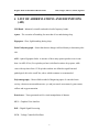
changes caused by higher stress levels. The respiration monitor is also a source of
uneasiness, as seen below in
Figure 1; It is a sensor that requires a tight, secure fastening around the chest, which is
understandably not comfortable.
Figure 1 - Sleep Study Patient in Full Gear
The specific values of interest that polysomnography collects for sleep apnea research are
brain waves, respiration, heart rate, and body movement. While brain waves cannot be
monitored without electrodes, it is ideal to find a way to monitor the other three without
making physical contact with the patient (in order to reduce stress and collect more
“natural” data). The development of such a product is the focus of this project.
7
Doppler Radar for Biomedical Measurements
Ball, Lamppa, Marrero, Selina, Sugimoto
6 Background Information on Doppler Radar Applied
to Apnea Studies
6.1 Doppler Radar
6.1.1 Radar Equation (RS)
The Doppler effect is defined as a shift in the frequency of a wave caused by the relative
motion of the transmitting source, the reflecting object, or the receiving system. The
Doppler effect will influence the data received from the radar in the following ways:
The Doppler Effect, or Doppler shift, can be described mathematically, as
follows:
f d=
2v r
λ
=
2v r f
C
o
where the v r is the relative velocity of the targets respect to the radar, f o is the
transmitted frequency, λ is wavelength and C is the velocity of radiation propagation.
6.1.2 Doppler Frequency and Phase Shift (RS)
In this project, any change in frequency will be unreadable due to its small size relative to
the carrier frequency. Respiration produces a contraction or expansion of the chest with a
velocity of less than 3cm/sec. The heart contracts at a typical rate of 6cm/sec. Inputting
this data into the radar equation yields:
fd =
1.03VT
λ
=
m
×2
0.1236
s
=
= 0.9888Hz
m
0.125
0.125
s
1.03 × 0.06
8
Doppler Radar for Biomedical Measurements
Ball, Lamppa, Marrero, Selina, Sugimoto
This Doppler shift will not be identifiable with a conventional VCO which will vary from
its center frequency.
Any observable information will be produced by a change in the phase shift between the
received and transmitted signals. How this phase shift is readable is shown below:
V( t ) cos ω1tV( r ) cos(ω 2t + φ )
= V( t )V( r ) [cos ω t cos ϕ − sin ω t sin φ ]cos ω t
= V( t )V( r ) [cos 2 ω t cos ϕ − sin ω t sin φ cos ω t ]
1
1
1
= V( t )V( r ) [ (1 + cos 2ω t ) cos ϕ − { sin(ω t − ω t ) + sin(ω t + ω t )}sin φ ]
2
2
2
1
1
1
= V( t )V( r ) [ cos ϕ + cos 2ω t cos ϕ − sin 2ω t sin φ ]
2
2
2
1
= V(t )V( r ) [cos ϕ + cos 2ω t cos ϕ − sin 2ω t sin φ ]
2
1
= V(t )V( r ) [cos ϕ + cos 2(2π f )t cos ϕ − sin 2(2π f )t sin φ ]
2
Where V(t ) cos ω 1t is the transmitted signal and V( r ) cos ω 2 (ω 2 t + φ ) is the received
signal. cos 2(2πf )t cos φ and sin 2(2πf )t sin φ are high frequency terms and are removed
by the low pass filter. As a result, only the phase component remains:
V = cos φ
6.2 Technical Contributions to Prototype (AB)
Biopac contributed their two functioning radar prototypes and the design of the 2.4GHz
radar to the project. They also supplied a copy of their AcqKnowledge data acquisition
software and the necessary MP100 acquisition hardware. The 2.4GHz radar design and
the AcqKnowledge MP100 system are used in the final prototype.
9
Doppler Radar for Biomedical Measurements
Ball, Lamppa, Marrero, Selina, Sugimoto
7 Apnea and Vital Signs Monitoring Subsystems
7.1 Antenna Array (AB)
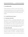
Our antenna array consists of two 2.4GHz radars mounted perpendicular to the subject
and sixty centimeters apart. They are positioned one meter from the subject. This distance
can be increased to two meters, though signal quality is degraded. A photo displaying a
test setup is shown below in Figure 2.
Figure 2 - Test Setup
The purpose of two antennas is to be able to have a signal reflected off the back of the
subject if they are lying on their side. Data quality is diminished when the subject is lying
on their side, but the respiration signal is of a higher magnitude when reflected off the
subject’s back. Two antennas allow us to collect data in this manner in a wider variety of
sleeping positions.
The 2.4GHz radar designed by Dr. Chip Scott for Biopac was never constructed. After
testing the prototype 1.85GHz and 900MHz units, a second 900MHz unit and two
10
Doppler Radar for Biomedical Measurements
Ball, Lamppa, Marrero, Selina, Sugimoto
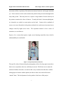
2.4GHz units were built to test an array configuration. The 2.4GHz units performed well
and were used throughout the project. A block diagram of the 2.4GHz radar units is
available below:
Figure 3 - Block Diagram for 2.4GHz Radar
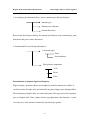
7.1.1 Transmitted and Received Signals (RS)
The radar will transmit a single frequency signal:
T (t ) = cos(2πft + φ (t ) )
where f is the oscillating frequency and φ(t) is the phase drift of the oscillator. The
received signal can be found as:
2d t −
R (t ) = cos 2πf t −
c
d (t )
c
2d t −
+ φ (t ) t −
d (t )
c
c
where c is the velocity of propagation and d(t) is the distance to the target. The signal will
be reflected by the target which is at a distance do. The total distance to the target will
11
Doppler Radar for Biomedical Measurements
Ball, Lamppa, Marrero, Selina, Sugimoto
also have a time varying displacement component x(t) which will consist of the vital
signs and any other movement. Thus the distance between the transmitter and receiver is
d(t)=do + x(t). After substituting this equality for d(t), the received signal becomes:
R (t ) = cos 2πft −
4πd o
λ
4πx t −
−
d (t )
c
λ
+φ t −
2d o
−
c
2x t −
d (t )
c
c
where λ=c/f. Since the period of oscillation for the vital signs is much larger than do/c and
x(t)<<do, we can approximate the received signal as:
R (t ) ≈ cos 2πft −
4πd o
λ
−
4πx(t )
λ
+φ t −
2d o
c
The received signal is similar to the transmitted signal with two differences. There is a
delay due to the distance do between the transmitter and the target and there is also a
phase change due to the periodic motion x(t). The mixer multiplies the received signal
with the local oscillator signal extracting the changing phase component. The resulting
signal can be characterized as:
B (t ) = cos θ +
4πx(t )
λ
+ ∆φ (t )
where:
12
Doppler Radar for Biomedical Measurements
∆φ (t ) = φ (t ) − φ t −
Ball, Lamppa, Marrero, Selina, Sugimoto
2d o
c
is the constant phase shift related to do and:
θ=
4πd o
λ
+θo
is the changing phase shift. Thus one can see that the respiration and heart rate signals
will be visible on the output of the mixer regardless of the fact that they do not produce a
Doppler shift [25].
7.1.2 Power Density Transmitted (KS)
Knowing that the vital signs should be present in the received signal, we need to confirm
that their magnitudes will be measurable. We determined the power density transmitted
by the radar and found that it is the maximum permissible under current ANSI/IEEE
regulations.
The power density of the radar is described as follows:
ρ=
{
}
G A P rad 1
= Re Ê ×Ĥ ∗ (W 2 )
m
2
4πr 2
This can be expanded to:
13
Doppler Radar for Biomedical Measurements
{
}
1
1
ρ ave = Re Ê ×Ĥ ∗ = Re Εˆ
2
=
2
2
Ball, Lamppa, Marrero, Selina, Sugimoto
2
1 r
1
1 r
a z = Re Εˆ m+1 (−0.72 − 0.034 j )
az
377
2
377
1 ˆ+
1
(Ε m1 (−0.72)) 2 (
) = 6.875 × 10 −4 (Εˆ +m1 ) 2 (W m 2 )
2
377
Where the intrinsic impedance of free space is:
ηˆ1 =
Εˆ
ˆ = 1 Εˆ
⇒Η
ˆ
377
Η
The transmitted wave from our antenna
Ε̂ +m1
is left as notation in this calculation
because Εˆ +m1 will vary depending on the antenna gain.
7.1.3 Reflected Energy (KS)
It is very important for the radar system to receive enough reflected energy so that
it is able to compare the differences between the RF and LO signals. For this reason, the
ratio of absorbed and reflected energy must be calculated.
The ratio of the energy that is reflected back from hitting a target is expressed in the
following equation.
Ê m1- = Ê m+1 (
ηˆ 2 −ηˆ 1
)
ηˆ 2 +ηˆ 1
Where ή is the intrinsic impedance of the objects:
14
Doppler Radar for Biomedical Measurements
ηˆ =
Ball, Lamppa, Marrero, Selina, Sugimoto
µ
∈− j
σ
ω
In this case, the boundary between free space and skin is used. For our research, the
parameters such as relative σ (conductivity), relative έ (permittivity), and relative µ
(permeability) of human skin are 1.0, 33, and 4π×10-7 respectively.
We obtained the ratio of
Εˆ m−1 =Εˆ m+1 (−0.72 − 0.034 j )
This result shows that around 70 percent of the energy is expected to be reflected back to
our radar. Supporting calculations are available in Appendix D.
7.1.4 Safety of Radiation (AB)
Radiation safety issues need to be considered when using radar on a human subject.
Radiation standards are governed by OSHA and standards have been set by IEEE and
ANSI. The primary health effect caused by non-ionizing radiation is heating when the
subject absorbs the transmitted energy. Prolonged radiation exposure above the OSHA
levels can produce adverse health effects. At the operational frequency of 2.4GHz,
radiation power density at the subject cannot exceed 2mW/cm2 based on the ANSI and
IEEE standard. Figure 4 is the IEEE standards of transmission.
15
Doppler Radar for Biomedical Measurements
Ball, Lamppa, Marrero, Selina, Sugimoto
Figure 4 - IEEE Standards for Frequency of Transmission
The power density (ρ) at the subject is as follows:
ρ=
{
}
G A P rad 1
= Re Ê ×Ĥ ∗ (W 2 )
2
m
2
4πr
Inserting values for the above we obtain:
ρ=
PG
t t
W m 2 = (−20 + 8 − (11 + 6.02))dB = −29.02 dB m 2 = 0.00125 w m 2
2
4π r
(
)
The IEEE/ANSI standard is:
F = 2m w cm 2 = 20 w m 2
The power density at the target is well below the maximum allowable levels of radiation.
16
Doppler Radar for Biomedical Measurements
Ball, Lamppa, Marrero, Selina, Sugimoto
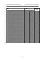
7.1.5 Radar Reliability (RS)
The mean time to failure (MTTF) for our two radar-antenna array is 7.07 years. This is
based on data obtained from an online component reliability database,
http://www.sercoassurance.com/the-srda/, and from Minicircuits, the manufacturer of the
used IC devices. Table 1 indicates the reliability data for a single radar antenna.
Component Failure Analysis
Component
JTOS-3000P
VNA-25
LAT-12
ALY-44MH
Description
Failure Rate
(per year)
VCO
Amplifier
Attenuator
Mixer
Variable Capacitor
Variable Resistor
Surface Mount Capacitor
Antenna
In-line Terminator (Resistor)
BNC to SMA Cables
Power Supply
MTTF (hours)
1887438
8760000
8760000000
2937784
0.00351
0.191
0.00181
0.00577
Failure Rate (per
million hours)
0.5298
0.1142
0.0001
0.3404
0.4007
21.8037
0.2066
6.6600
0.6587
0.0014
1.5800
Total Failure Rate:
(per million hours)
MTTF (Hours):
MTTF (Years):
Table 1 - Component by Component Failure Data
The mean time to failure for a single radar unit is 3.53 years. However, since we are
using two radar devices that can work independently, the system MTTF is 7.07 years.
17
32.2955
30964.0412
3.5347
Doppler Radar for Biomedical Measurements
Ball, Lamppa, Marrero, Selina, Sugimoto
The system is redundant because should one device malfunction, the other would still
collect valid data.
The MTTF for these designs is lacking, and largely cut short by the failure rate of the
variable resistor. There is also a design flaw on the existing prototypes related to this
resistor. The potentiometer will short out the power supply when adjusted to zero ohms,
since there is no additional resistance in series with the potentiometer to prevent current
flow. This causes the monolithic amplifier in the circuit to fail.
7.2 Radar Data Acquisition and Signal Processing (NM)
Our Data Acquisition and Signal Processing System consists of two steps. The data is
collected using Biopac’s provided MP100 system in real time and then post processed
using a team-generated Matlab program (GUI).
7.2.1 The MP100 and AcqKnowledge (NM)
AcqKnowledge and the associated MP100 hardware are used to digitize the data and save
it as a text file for future manipulation. AcqKnowledge is Biopac’s proprietary data
acquisition system and it has more functionality than is required for this application. The
Biopac resources are for proof of concept; any future marketable version of this prototype
will include a much simpler data acquisition system that lacks almost all of the functions
of the AcqKnowledge program.
18
Doppler Radar for Biomedical Measurements
Ball, Lamppa, Marrero, Selina, Sugimoto
Regardless of the final program used to sample data, our created processing system
requires a text file input consisting of two to four tab-delineated columns, each
corresponding to one set of sampled. In the final phase of our product, the input to the
Matlab program only consists of the two radar channels in two columns. For data
validity verification purposes, heart and respiration control rates can be received as well
in the other two channels (columns of data). The input data needs to be consisting of 200
samples a second (200Hz) for accurate analysis in the processing system of the Matlab
program.
7.2.2 Matlab and Algorithms (NM)
The data collected using AcqKnowledge is post processed in Matlab. The raw feeds from
both radars are received and the following are extracted:
•
Heart Rate Signal
•
Respiration Rate Signal
•
Movement Signal
The numeric heart rate, respiration rate, the magnitude and duration of motion and
occurrences of apnea. The Graphical User Interface (GUI) is a final version of a test
program written for the project called the Dataviewer.
19
Doppler Radar for Biomedical Measurements
Ball, Lamppa, Marrero, Selina, Sugimoto
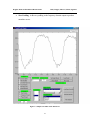
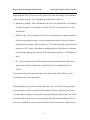
7.2.3 Dataviewer (NM)
For visual manipulation of the data, a user-controllable program called Dataviewer was
created to test the algorithms written for the project. It has the capability to display any
portion of any channel in the time domain, frequency (magnitude) domain, and the phase
domain. It also has numerous other functions that will be individually described below.
Figure 5 on page 21 shows a screenshot of the Dataviewer.
Datasets are loaded in via the “Load Data From File” button (see Figure 5). The
main window of the dataviewer is the graphical display, presenting the data from the
selected channel over the window. The window is fully scalable by using the mousecontrolled zoom function inherent in Matlab plots. This allows a user to investigate data
in detail. For the time domain, the x-axis is always in terms of seconds, referenced from
the start of the data collection, and the y-axis is the voltage of the signal. For the
frequency (magnitude) domain, the x-axis is expressed in Hz for ease of recognition of
the characteristic signal peaks.
The six checkboxes on the left below the window (labeled ‘Options’) are
functions that allow a user to further explore the datasets:
•
Hold Enabled: Should a user wish to overlay two different channels for a more
direction comparison, he should use the Hold function. This holds whatever
datasets are currently displayed is in the window and plots the next selected
dataset over it. This can be repeated indefinitely.
20
Doppler Radar for Biomedical Measurements
•
Ball, Lamppa, Marrero, Selina, Sugimoto
Zero Padding: Adds zero padding to the frequency domain output to produce
smoother curves.
Figure 5 - Sample Screenshot of the Dataviewer
21
Doppler Radar for Biomedical Measurements
•
Ball, Lamppa, Marrero, Selina, Sugimoto
DC Offset Removal: This subtracts from the dataset (or time window) the mean
of the set. This removes the DC component, which appears as a large peak at 0
Hz in the Frequency magnitude domain. Removing this large peak makes
displaying the rest of the frequency components easier.
•
Time Windows: This function allows a user to divide the dataset into windows of
a user-defined length and select any portion of it for display. This is helpful to
simulate the window-by-window data-processing algorithms, and to look at the
characteristics of a smaller portion of the data.
•
Normalize Data: When comparing two sets of data using the hold function, the
data can be of different magnitudes. Using this function, one can define the
normalization factor to which the dataset is scaled to, allowing overlapping
comparison between datasets.
•
Peak Detection: This is the peak finding algorithm used in the respiration- and
pulse-rate finding algorithms. It analyzes the windowed data and finds the
relative peaks throughout, placing a mark on each. This is best used with the hold
function on, so that the peaks can be overlaid on the original graph.
Below “Options” is the “Domain” section, which allows a user to select the domain that
the plot displays. The sampling frequency below is used to calculate the time and
frequency index used in the plots; obviously, data sampled at a frequency of 100 Hz
could not be displayed accurately on the same time index as that of a 200 Hz dataset. To
the right of that is the channel select, in which a user can choose the channel to be
displayed. To the right of the channel select is the filter selection, in which standalone
22
Doppler Radar for Biomedical Measurements
Ball, Lamppa, Marrero, Selina, Sugimoto
filter programs can be dropped in and applied to the data. Standard filters, like the
Butterworth low pass filter, and special filters, like a manual version of the respirationrate finding algorithm, are found in here and can be applied to a given dataset.
The “Load Script” and “Run Script” functions allow a user to employ scripts that
automatically use all the previously described functions to display a complex product;
one such script included with the Dataviewer, CheckRespiration, is an automated version
of the respiration-rate finding algorithm, using the Dataviewer functions.
Most of these functions are implemented by the back-end of the GUI
automatically. These algorithms are discussed in more detail in the following sections.
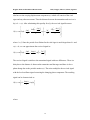
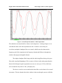
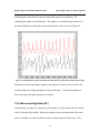
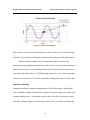
7.2.4 Respiration (DL)
The radar waves pick up a phase shift as they encounter the moving chest cavity; this
phase shift is dependent on the relative velocity of the chest when the transmitted wave
encounters the boundary of the chest. This phase shift is responsible for the appearance
of the respiration rate in the sampled waveforms.
To understand what sort of periodic signal to extract from the sampled radar data,
it is helpful to have a reference signal that is the exact respiration signal. To this end,
Biopac provided a pressure sensitive sensor that wraps around the chest and creates an
output voltage based on the chest cavity movement. Figure 6 shows the use of the
Dataviewer to overlay the radar signal over the control respiration signal for a given time
window. The red curve is the radar data and the black is the reference signal data.
23
Doppler Radar for Biomedical Measurements
Ball, Lamppa, Marrero, Selina, Sugimoto
Figure 6 - Control Respiration (Black) vs. Radar Signal (Red)
The radar data was normalized for a better visual comparison. Looking at Figure 6, it is
clear that the radar carries the respiration rate data. In order to extract the pure
waveform, an adaptive bandpass filter was created, which locates the characteristic
frequency peak of the respiration in the frequency domain and follows it through time
windows that progress through the dataset.
The adaptive bandpass filter beings with, the data being filtered using a low pass
filter with a stop band beginning at 3Hz, to remove all noise in the radar greater than the
limits of the biological signals (respiration can occur at a rate up to 1.2 Hz, while heart
rate is assumed to stay below a 3Hz [180 bpm] rate).
The data is viewed in a ten second window that slides over the data in five-second
increments. The time domain data in the window is then run through a process called the
24
Doppler Radar for Biomedical Measurements
Ball, Lamppa, Marrero, Selina, Sugimoto
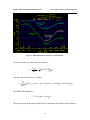
Fast Fourier Transform (FFT), which yields a set of complex numbers containing the
frequency, magnitude and phase responses of the data in the time window. The
magnitude response is of interest, because it is here that the characteristic frequency peak
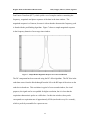
is found with the peak finding algorithm. Figure 7 shows a sample magnitude response
in the frequency domain of an average time window.
Figure 7 - Sample Radar Magnitude Response for a 10-second Window
The DC component has been removed using the DC offset algorithm. The DC bias in the
radar data comes from the bleed-through from the LO to the RF input of the mixer on the
radar device hardware. This resolution is typical of a ten-second window; for visual
purposes, the signal can be zero-padded for higher resolution, but it is clear that the
respiration characteristic peaks are visible here. In this time window, these peaks
correspond to a respiration rate of approximately 0.2Hz (one breath every five seconds),
which is perfectly reasonable for a person at rest.
25
Doppler Radar for Biomedical Measurements
Ball, Lamppa, Marrero, Selina, Sugimoto
Because the time window is a rectangular function being applied to a specific
portion of the dataset, one may expect to see sidelobe leakage in the frequency domain
[22]. This is typically something to be concerned about, and using a Blackman or
Hanning window instead of a rectangular window can diminish this effect. However, for
the purposes of this project, it is not necessary. There is not significant energy leakage to
make these peaks indistinguishable; they are simply too significant to be lost in the
leakage.
This characteristic frequency peak is easily found with the peak-finding
algorithm. This frequency becomes the center of the bandpass filter, whose transition
bands are then placed on the nearest relative minima on either side of the peak. This
band of data can then be put back in the time domain via the Inverse Fast Fourier
Transform (IFFT) and displayed for each window. The phase shift is still present in the
extracted respiration from the radar, but only visible when compared directly to the
control respiration signal. By averaging the respiration frequency (the main peak) for the
time windows in a given time spread, we can easily determine the respiration rate for a
whole dataset or any subset therein.
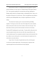
Figure 8 shows 50 seconds of original radar data, in blue, while the purple
waveform is the isolated respiration data. The main frequency component of the
respiration signal has been extracted and can be clearly displayed.
26
Doppler Radar for Biomedical Measurements
Ball, Lamppa, Marrero, Selina, Sugimoto
Figure 8 - Original Radar (Blue) with Extracted Respiration (Purple)
This algorithm proves to be very robust in finding the respiration from the radar data
under all conditions and positions of the body beneath the radar antenna system. When
apnea episodes occur in the same time window, the frequency response is not drastically
affected; the apnea effects, which appear as noise because respiration stops (leaving only
pulse data and system noise). This is effectively zero padding, having minor influence on
the magnitude of the very low frequency components.
7.2.5 Heart Rate (DL)
The pulse rate is picked up by the reflection of the RF energy off the periodically varying
position of the heart as it beats. Because the radiated energy has numerous boundaries to
interact on the approach and return path from the heart (skin, ribs, cartilage, blood, and
27
Doppler Radar for Biomedical Measurements
Ball, Lamppa, Marrero, Selina, Sugimoto
fat), and it also is hitting a moving target with smaller total displacement, the returned
pulse signal is understandably much smaller than the respiration signal. The respiration
amplitude is, on average, one hundred times larger than that of the pulse amplitude. This
makes isolating the heart rate more difficult, and a different approach is required. The
amplitude of the noise from the system also makes it more difficult to discern the pulse
rate from the signal, since the ambient noise is of approximately the same amplitude.
Once again, it is helpful to have a reference signal against which to compare the
time-varying reflected waveforms. Biopac provided a sensor for this purpose, one that
detects changing densities in blood in the tip of a finger. Figure 9 shows a reference
signal response and its characteristic magnitude response in the frequency domain.
Figure 9 - Control Pulse in Time (left) and Frequency Magnitude Response (right)
One expects the pulse signal to appear periodic, and it does. What was unexpected was
the harmonic nature of the magnitude response. The first and second harmonics
occurring roughly two and three times above the characteristic peak frequency. They
appear as a result of the density variances in the blood that the sensor picks up. To
extract a similarly appearing pulse signal from the radar, these signals must be
28
Doppler Radar for Biomedical Measurements
Ball, Lamppa, Marrero, Selina, Sugimoto
approximated from the radar signal. However, the radar does not pick up these
harmonics, and so they will have to be artificially created from the ambient noise
occurring at these frequencies. First, though, a general discussion of extracting the pulse
signal from the radar follows.
Because the pulse signal is a few orders of magnitude smaller than the respiration
signal, the respiration frequency data must be removed before pulse analysis can begin.
The lower-frequency, higher-magnitude respiration signal is cut off with a lowpass filter
with a stop band up to 1 Hz. The resulting signal then has a lower average amplitude and
is fitted for analysis. Next, the positive and negative peaks of the 1 to 3Hz range (relative
maxima and minima respectively) are found and tallied. The positive peaks are sorted
and the peak ratio (the ratio of one peak’s amplitude to the next) is considered. If this
peak ratio is greater than 0.5, then the peaks are not far enough apart. The pulse
characteristic frequency peak stands above the surrounding noise by about 4 times larger,
so that when the highest ratio (differential) is seen, the initial peak is treated as our
characteristic frequency peak of the pulse data. Once this peak is located, the two
surrounding relative minima become the cutoff bands of the adaptive bandpass filter that
follows the main component of the pulse signal. Once again, this signal is IFFTed and
displayed in the GUI.
This only reproduces a single sine wave that contains the main frequency
component of the pulse (similar to Figure 8, the respiration signal). To generate a signal
that looks more like the reference pulse, the harmonics have to be artificially induced.
The radar does not pick up the harmonics from the interaction with the movement of the
heart, so a technique must be created to simulate their presence. This is done by
29
Doppler Radar for Biomedical Measurements
Ball, Lamppa, Marrero, Selina, Sugimoto
multiplying the characteristic frequency bandwidth range by two and three, and
amplifying the signal noise held therein. This produces a reasonable approximation of
the natural harmonics of the pulse signal and yields the results, as seen in Figure 10.
Figure 10 - Resulting Pulse signal extracted from radar (Black) Against Control Pulse Sensor (Red)
With these two basic algorithms complete, the project was ready to move into the casespecific design of creating a program for sleep monitoring. To do this, algorithms to
detect movement and apnea episodes are required.
7.2.6 Movement Algorithm (DL)
Unfortunately, one aspect of conducting a sleep study on a fully mobile patient is that he
or she is just that: fully mobile. Because the patient is not movement-limited by sensor
gear or restraints, he is able to exhibit normal movement patterns during sleep. This
30
Doppler Radar for Biomedical Measurements
Ball, Lamppa, Marrero, Selina, Sugimoto
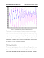
movement effectively nullifies the radar data during the movement and for a period
afterwards. Figure 11 shows a sample radar waveform that has movement data. When the
subject moves, he or she causes abrupt amplitude jumps and uncharacteristic frequency
response. Note that after the movement episode, the data does not immediately settle
back down into the predictable periodic signal that it used to be. On average, it takes two
to three seconds to fully reacquire the respiration and pulse rates.
Figure 11 - Data Collection Interrupted by Subject Movement
To effectively tally these regions in a collected set of data so that the other
algorithms won’t consider them, a movement locating algorithm had to be created. This
algorithm is to go through the radar datasets and mark sections of the data that are
movement. To accomplish this, the function is passed anywhere from a small time
window to the whole data set, which parses the passed subset into an X by 200 matrix,
where X is the number of seconds in the data. The maximum and minimum values for
31
Doppler Radar for Biomedical Measurements
Ball, Lamppa, Marrero, Selina, Sugimoto
each second are found and stored. Then, the mean of each second is stored in an array.
For any given second, if the maximum or minimum peak is above or below the average
by a given threshold, the second is marked as containing movement. The function then
tallies the number of seconds in a row that are marked, and outputs the duration of the
movement as well as the start of movement (the second it started, based within the data
timestamp reference).
The function has a few additions in it to assure robust operation. First, since there
may be a case where a second of data is characterized by the downward drop of a
periodic signal (which may be outside the governing thresholds), any cases of movement
that only last one second are disregarded. Also, if in the middle of a string of seconds of
movement, should one second inside the string not meet the criteria to be considered
movement, it is assumed to be inside a longer string of movement. For example, should
2 seconds of movement and 3 seconds of movement be separated by one second that does
not register as movement, they are all output as one six-second episode of movement.
The output is sent to the GUI, which isolates these ranges from the radar data and
displays them in the movement channel of the GUI. The GUI backend also makes note
of these ranges for use by the other algorithms, which disregard them in their processes.
32
Doppler Radar for Biomedical Measurements
Ball, Lamppa, Marrero, Selina, Sugimoto
7.2.7 Apnea Episodes (RS)
In the radar signal data set, an apnea episode is characterized by the disappearance of the
respiration signal for a ten-second interval. As a result, the amplitude variations of the
radar drop significantly and the signal is reduced to the heart rate and the system noise.
Figure 12 shows the control respiration sensor picking up an apnea event (red), while the
black curve is the raw radar data feed. The apnea episode occurs between 30 and 40
seconds.
Figure 12 - Apnea Episode from Control Sensor and Radar Signal
33
Doppler Radar for Biomedical Measurements
Ball, Lamppa, Marrero, Selina, Sugimoto
Since the large signal of the respiration has disappeared, the radar signal only varies by
fractions of what it once did. As a result, a modification of the movement algorithm can
be used to determine the starting time and duration of apnea episodes. The beginning of
the algorithm is still the same; the signal is partitioned into one second increments and
analyzed. The average value, maximum, and minimum peaks for each second increment
are also found.
Similar to the movement algorithm, the average value and the maximum and minimum
peaks are compared, but for the case of apnea, the peaks must be within a certain
bandwidth threshold. That is, if a given second has both its maximum and minimum
peaks within 0.1 of the average value for the second, it is safe to conclude that there is no
respiration component present and that it may be part of an apnea episode (thus raising a
flag for the second). Using the tallying system of the movement algorithm, if ten or more
consecutive seconds occur with raised flags, then the time set is considered to be an
episode of apnea. It is considered as such until two consecutive seconds have lowered
flags; then the apnea episode has a beginning time index, length, and an ending time
index.
Once a dataset has been analyzed in this manner, the total number of episodes are
counted up and divided by the total length of the data set in hours. This number is then
displayed in the GUI as the Apnea-Hypopnea Index (AHI). This is the tell-all signifier
that indicates whether or not a patient has a diagnosable level of sleep apnea.
34
Doppler Radar for Biomedical Measurements
Ball, Lamppa, Marrero, Selina, Sugimoto
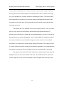
7.3 GUI Overview - Data Display and Manipulation (NM)
The GUI serves as an interface between the user and the algorithms developed to extract
signals from the radar data. From the standard Windows interface menus (Figure 13), the
user can load a saved data set, save a processed data set, close the current data set, print
the current data set, exit the program, modify patient information, modify the data display
axes, obtain help on using the GUI, obtain version information about the GUI, or put the
GUI in a special operating mode called Debug Mode.
Figure 13 - Standard Windows Menu Interface in the GUI
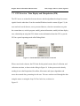
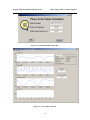
When a user loads a data set, the GUI asks for the patient’s name, date of collection, and
collection start time, as shown in the dialog in Figure 14. It then processes the data by
sending it out to the Respiration, Heart Rate, Movement, and Apnea algorithms and
stores the returned data, presenting it to the user. The user can then scroll through the data
using the mouse or using the Jump To Time Index box, as shown in
Figure 15.
35
Doppler Radar for Biomedical Measurements
Ball, Lamppa, Marrero, Selina, Sugimoto
Figure 14 - Patient Information Dialog Box
Figure 15 - A Screenshot of the GUI
36
Doppler Radar for Biomedical Measurements
Ball, Lamppa, Marrero, Selina, Sugimoto
When using the Jump To Time Index box, the user can enter time indices in five manners
(where d stands for digit – [0-9]): dd:dd:dd, d:dd:dd, dd:dd, d:dd, or d+.
Dd:dd:dd or d:dd:dd – This is translated by the GUI to be absolute time. For example,
if a dataset begins at 21:00 and the user enters 22:35:00, it would move to 1:35:00
into the data.
Dd:dd or d:dd – This is translated by the GUI to be absolute time without seconds for
data sets longer than one hour, or as only minutes and seconds for data sets within a
single hour. For example, if the user enters 15:15 in a data set within an hour, the data
moves to h:15:15, where h is the hour in which the data set falls. However, if the data
set were longer than an hour, then the GUI would interpret that as 15:15:00 and move
there.
D+ - This is translated by the GUI to mean seconds from the start of the data. If the
data started at 1:00:00 and the user entered 350, the GUI would display data at
1:05:50.
If any of these times fall outside the range of the data, then the GUI will move as far
towards these times as the data allows.
When displaying data, the GUI automatically adjusts the y-axis of the viewing windows
to show the data as large as possible for that window. Because of this, the y-axis of the
viewing windows changes every time the data being displayed changes. If the user wishes
to stop this behavior, the Freeze Axes menu under the Edit menu holds indicators for all
four axes. In addition, the user can Freeze/Unfreeze all four axes at once. When an axis is
37
Doppler Radar for Biomedical Measurements
Ball, Lamppa, Marrero, Selina, Sugimoto
frozen, its minimum value stays at the minimum value of the entire dataset, likewise for
maximum.
Three additional features incorporated into the GUI are:
•
The ability to modify patient information (under the Edit menu) if a mistake is made
initially.
•
The ability to modify the sampling rate, if it is other than the default 200 Hz. This is
done in the Scan Rate input box.
•
The ability to create Debug logs that are helpful in troubleshooting or modifying the
functionality of the GUI.
The Debug Mode of the GUI produces an output file (GUIDebug.txt) which will show
the reader what callbacks and subroutines the GUI is in along with any pertinent data
about variables in those routines. With access to the debug file and the source code for
the GUI, debugging any errors that arise should take much less guesswork than standard
debugging.
Figure 16 - An Example of User Oversight
38
Doppler Radar for Biomedical Measurements
Ball, Lamppa, Marrero, Selina, Sugimoto
In addition, the GUI contains some limited user oversight (program redundancies to
prevent a user from losing data). For example, if the user closes a file before saving it, the
GUI asks the user if they wish to save the current data set. In Figure 16, the user is asked
to confirm if they want to exit the program. If the user enters values incorrectly that the
system needs to understand a request (in the Jump To Time Index or Patient Information
Start Time boxes for example) then the GUI will display an error message. In some cases,
the GUI will simply not comply. In these cases, the Debug Mode output file will contain
more specific error messages.
Code for the GUI is available in the Digital Appendix CD-ROM.
39
Doppler Radar for Biomedical Measurements
8
Ball, Lamppa, Marrero, Selina, Sugimoto
Recommendations for Future Work (RS)
The prototype fulfills its intended function but is lacking in the following regards:
•
Bulky Hardware and Inconvenient Setup
•
Hardware Design Flaw
•
Poor Heart Rate Recognition
•
Nulls in Range
•
Post Processing
Bulky Hardware
The necessary acquisition hardware and PC make this setup impractical. In addition, the
AcqKnowledge data acquisition system is much more complex than what is necessary for
the application. A smaller and simpler data acquisition system designed for this
application would make the system more economical and practical to setup. An ideal
feature would be onboard memory to store the night’s data for later analysis. In addition,
it would be appropriate to develop a stand that can be adjusted in width and height to
setup the radar antennas in a person’s home for a temporary installation.
Hardware Design Flaw
The potentiometer on the radar boards will short out the power supply when adjusted to
zero ohms, since there is no additional resistance in series with the potentiometer to
prevent current flow. This causes the monolithic amplifier in the circuit to fail. Two fixed
resistors arranged as a voltage divider could provide the target control voltage without the
use of the potentiometer in future prototype models. Not only would this eliminate the
flaw, but it would also replace the least reliable component present in the prototype and
increase the MTTF per unit to 10.88 years, increasing the system MTTF to 21.76 years.
40
Doppler Radar for Biomedical Measurements
Ball, Lamppa, Marrero, Selina, Sugimoto
Poor Heart Rate Recognition
The heart rate signal is very difficult to locate in the radar data. Noise from surrounding
electronics and from drift with the VCO make the characteristic frequency peak nearly
impossible to distinguish from noise in the signal. A more accurate VCO and a less noisy
environment could make this data more visible.
Nulls in Range
When the local oscillator and the received signal are either 0 or 180 degrees out of phase,
null points occur. Thus nulls are found with a target distance of λ/4 from the radar. With
our transmitted frequency of 2.4GHz, these nulls occur every 3cm, which makes them
nearly impossible to avoid when monitoring a patient.
A quadrature radar transceiver can eliminate these null spots and would be a valuable
improvement on the existing radar hardware. Information on a quadrature receiver
designed for vital signs monitoring can be found in the IEEE paper “Range Correlation
and I/Q Performance Benefits in Single-Chip Silicon Doppler Radars for Noncontact
Cardiopulmonary Monitoring” by Droitcour et al.
Post Processing
Post-processing was determined to be acceptable for this application. Should the system
be modified to run in real-time however, it could be made substantially more versatile
and could be used in applications such as infant monitoring to prevent sudden infant
death syndrome.
41
Doppler Radar for Biomedical Measurements
Ball, Lamppa, Marrero, Selina, Sugimoto
9 APPENDICES
APPENDIX TITLE
SECTION
References
A
Budget
B
Timeline
C
Reflection and Absorption Supporting Calculations
D
Permittivities and Conductivities of Biological Tissue
E
Interactions of RF Energy and Biological Tissues
F
Breakdown of the Radar Front-End Components
G
Radar Evaluation and Design
H
Digital Appendices
I
42
Doppler Radar for Biomedical Measurements
Ball, Lamppa, Marrero, Selina, Sugimoto
9.1 Appendix A - References
1. http://www.sleepnet.com/sleepapnea.html
2. http://www.lungusa.org/diseases/sleepapnea.html
3. http://www.sleepapnea.org/slpaprsk.pdf
4. http://www.sleepclinic.org/apnea.html
5. http://classes.kumc.edu/cahe/respcared/cybercas/sleepapnea/trenpoly.html
6. http://www.talkaboutsleep.com/sleepbasics/viewasleepstudy.html
7. http://hyperphysics.phy-astr.gsu.edu/hbase/sound/wavplt.html#c2
8. Balakrishnan, A. V. Kalman Filtering Theory. New York: Optimization Software,
1987.
9. Baranski, S. and P. Czerski. Biological Effects of Microwaves. Pennsylvania:
Dowden, Hutchinson & Ross, 1976.
10. Battocletti, Joseph H. Electromagnetism Man and the Environment. Boulder:
Westview Press, 1976.
11. Chen, Kun-Mu, et al. “An X-Band Mircrowave Life Detection System.” IEEE,
1986.
12. Droitcour, Amy, et al. “A Microwave Radio for Doppler Radar Sensing of Vital
Signs.” IEEE, 2001.
13. Edmonds D. T. Electricity and Magnetism in Biological Systems. New York:
Oxford, 2001.
14. Embree, Paul M. and Bruce Kimble. C Language Algorithms for Digital Signal
Processing. New Jersey: Prentice Hall, 1991.
15. Johnk, Carl T.A. Engineering Electromagnetic Fields and Waves. New York:
John Wiley & Sons, 1988.
16. Lohman, B, et al. “A DSP for Doppler Radar Sensing of Vital Signs.” IEEE,
2002.
17. Polk, Charles and Elliot Postow. Handbook of Biological Effects and
Electromagnetic Fields. Florida: CRC Press, 1986.
43
Doppler Radar for Biomedical Measurements
Ball, Lamppa, Marrero, Selina, Sugimoto
18. Proakis, John G. and Dimitris G. Monolakis. Digital Signal Processing:
Principles, Algorithms and Applications. New Jersey: Prentice Hall, 1996.
19. Ramachandra, K.V. Kalman Filtering Techniques for Radar Tracking. New York:
Marcel Dekker, 2000.
20. Stearns, Samuel and Ruth A. David. Signal Processing Algorithms in Matlab.
New Jersey: Prentice Hall, 1996.
21. Yuen, C.K. and D Fraser. Digital Spectral Analysis. California: CSIRO, 1979.
22. Proakis, John G., Dimitris G. Manolakis. Digital Signal Processing: Principles,
Algorithms, and Applications, Third Edition. Prentice Hall, New Jersey. 1996.
23. DeMaw, Doug. Practical RF Design Manual. Prentice-Hall, New Jersey. 1982.
24. Prat, Timothy et al. Satellite Communications. Wiley & Sons. 2003.
25. Droitcour, Amy et al. “Range Correlation and I/Q Performance Benefits in
Single-Chip Silicon Doppler Radars for Noncontact Cardiopulmonary
Monitoring” IEEE. 2004.
26. www.radiolab.com
44
Doppler Radar for Biomedical Measurements
Ball, Lamppa, Marrero, Selina, Sugimoto
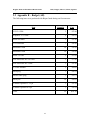
9.2 Appendix B – Budget (AB)
The following items were purchased with Biopac funds during our first semester:
Item
Quantity
Cost
VCO 2.4 GHz
2
$53.90
Amplifier .5-2.5 GHz
6
$29.70
Mixer 900 MHz
2
$35.90
VCO 900 MHz
2
$49.90
Attenuator 12dB
10
$19.50
Attenuator 15dB
10
$19.50
Mixer 2.4 GHz
2
$37.90
Low Pass Filter DC-2.95 GHz
2
$73.90
Low Pass Filter DC-1 GHz
2
$25.90
2.4 GHz Antenna
2
$95.00
SMA plug
3
$36.12
SMA to BNC plug
3
$32.73
10
$44.50
Variable Capacitor .3-1.2 pF
2
$25.98
Variable Capacitor .8-8 pF
1
$15.28
59
$611.26
SMA jack
Total:
45
Doppler Radar for Biomedical Measurements
Ball, Lamppa, Marrero, Selina, Sugimoto
In addition to these items, we also purchased the following using NMT funds:
Item
Quantity
Cost
ROS-960PV VCO
2
$19.95
VNA-25 Amplifier
4
$4.70
RMS-5H Mixer
2
$16.85
BLP-150 LP Filter
2
$32.95
Parts Bin
1
$12.00
Tin Foil
1
$3.00
Freight Charges
$38.49
Total:
8
$211.79
We also received 5 additional LAT-12 attenuators from Minicircuits, and three variable
capacitors from Mouser Electronics free of charge.
46
Doppler Radar for Biomedical Measurements
Ball, Lamppa, Marrero, Selina, Sugimoto
9.3 Appendix C - Project Timeline (DL)
Task
Manpower
Hours
Date
Start
Documentation
Statement of Work
Preparation for Conceptual Design Review
Conceptual Design Review
Preparation for Preliminary Design Review
Preliminary Design Review
Preparation for Critical Design Review
Critical Design Review
Write Formal Report
Formal Report
Preparation for Thesis
Thesis
Thesis Presentation Preparation
Thesis Presentation
10/01/03
10/01/03
10/07/03
10/07/03
10/21/03
10/21/03
11/04/03
11/15/03
12/03/03
03/15/04
04/20/04
04/20/04
04/30/04
Doppler Front End
Consult w/ Dr. Scott on Existing Designs
Training w/ Alan Macy and Dr. Scott
Purchase 2.5 GHz Prototype Supplies
Evaluate 1900 Mhz Unit
Evaluate 900 MHz Unit
Investigate Antenna Design
Investigate Antenna Purchase Options
Determine Conceptual Antenna Design
Refine Antenna Array Design
Determine Final Array Configuration
Build 2.5GHz Prototypes and 900MHz Prototypes
Build Antenna Mounting Hardware
Test Antenna Array Design
Collect Small Apnea Data Sets
Collect Abnormal Data Sets
Collect Movement Data Sets
Collect Long Apnea Data Sets
Collect Long Sleeping Data Sets
13/03/03
10/09/03
10/09/03
10/10/03
10/10/03
10/10/03
10/10/03
11/04/03
11/04/03
12/03/03
12/04/03
12/04/03
12/26/03
02/27/04
02/27/04
02/27/04
03/19/04
03/19/04
47
End
10/07/03
60
60
10/21/03
60
11/04/03
60
12/03/03
120
04/20/04
120
04/30/04
11/04/03
11/04/03
11/03/03
11/01/03
8
8
20
20
20
40
40
12/02/03
20
12/23/03
12/23/03
01/07/03
40
2
20
2
10
2
6
6
Doppler Radar for Biomedical Measurements
Ball, Lamppa, Marrero, Selina, Sugimoto
Task
Date
Manpower
Hours
Start
End
DSP Engine
Investigate Existing Techniques and Methods
Evaluate DSP engine with new 2.5 GHz Front End
Determine needed DSP Engine Specs
Determine Hardware or Software Implementation
Determine Preliminary Design
Programming Initial Single Antenna Program
Develop Respiration Algorithm
Test Respiration Algorithm
Develop Heart Rate Algorithm
Test Heart Rate Algorithm
Develop Movement Algorithm
Test Movement Algorithm
Develop Apnea Algorithm
Test Apnea Algorithm
10/10/03
11/20/03
11/02/03
11/02/03
11/02/03
12/03/03
03/01/04
03/02/04
03/01/04
03/19/04
03/19/04
04/14/04
03/19/04
04/19/04
12/03/03
11/25/03
GUI System
Investigate Existing Techniques and Methods
Evaluate Existing GUI
Determine needed GUI Specs
Determine Redesign or Modification
Determine Preliminary Design
Preliminary Front End Done
Final Front End Done
Back End Development
Back End Complete
10/10/03
10/10/03
11/02/03
11/02/03
11/02/03
12/03/03
03/22/04
03/22/04
04/20/04
System Integration
Incorporate GUI, DSP Engine and Radar
Prototype Finished
Deliver Prototype
02/01/04
04/01/04
05/01/04
48
03/19/04
03/19/04
04/20/04
04/14/04
04/20/04
04/19/04
04/20/04
40
20
60
10
60
100
40
10
40
10
20
10
20
10
11/02/03
11/02/03
40
20
12/03/03
03/22/04
04/20/04
04/20/04
20
80
100
100
02/20/04
04/20/04
04/30/04
40
12/03/03
01/07/04
Doppler Radar for Biomedical Measurements
Ball, Lamppa, Marrero, Selina, Sugimoto
9.4 Appendix D - Reflection and Absorption Supporting
Calculations (KS)
The complex amplitude of the reflected wave
Intrinsic wave impedance of free space
ηˆ 1 =
µ
∈− j
σ
ω
=
4π × 10 −7
=
10 −9
0
−j
36π
2π (2.5 × 10 9 )
(4π × 10 −7 )
= 142122 ≅ 377
10 −9
36π
Intrinsic impedance of skin
ηˆ 2 =
=
µ
∈− j
σ
ω
=
4π × 10 −7
10 −9
1
(33 ×
)− j
36π
2π (2.5 × 10 9 )
=
4π × 10 −7
2.92 × 10 −10 − j1.59 × 10 −10
(4π × 10 −7 )(2.92 × 10 −10 + j1.59 × 10 −10 )
=
(2.92 × 10 −10 − j1.59 × 10 −10 )(2.92 × 10 −10 + j1.59 × 10 −10 )
= 3.321 × 10 3 + j1.8 × 10 3
1
2
1
2
(a + jb) = r e
1
j θ
2
r = 1.1 × 10 7 + 3.24 × 10 6 = 1.42 × 10 7 = 3.77 × 10 3
θ = tan −1 (
− 3.24 × 10 6
) = tan −1 (−2.945 × 10 −1 ) = −16.41
1.1 × 10 7
Polar Form
1
2
ηˆ 2 = (3.77 × 10 ) e
3
1
j ( −16.41)
2
= 61.4e j 8.205
49
(3.67 × 10 −16 + j1.998 × 10 −16 )
(8.526 × 10 − 20 − 2.53 × 10 − 20 )
Doppler Radar for Biomedical Measurements
Ball, Lamppa, Marrero, Selina, Sugimoto
Trigonometric Form
ηˆ 2 = 61.4e j 8.205 = 61.4(cos(−8.205) + j sin( −8.205)) = 61.4(0.989 + j (−0.143))
= 60.72 − j8.76
ηˆ 2 −ηˆ 1 60.72 − j8.76 − 377 − 316.28 − j8.76 (−316.28 − j8.76)(437.72 + j8.76)
=
=
=
)
437.72 − j8.76
(437.72 − j8.76)(437.72 + j8.76)
η 2 +ηˆ 1 60.72 − j8.76 + 377
=
− 138422 − j 2770.6 − j 3834.42 + 76.737 − 138345 − j 6605
=
= −0.72 − j 0.0344
191598.8 + 76.737
191675.5
Therefore the calculation below shows around 72% of energy will be reflected back.
Ê m1- = Ê m+1 (−0.72 − j 0.0344)
50
Doppler Radar for Biomedical Measurements
Ball, Lamppa, Marrero, Selina, Sugimoto
9.5 Appendix E - Permittivity and Conductivity of Biological
Tissue as a Function of Frequency
51
Doppler Radar for Biomedical Measurements
Ball, Lamppa, Marrero, Selina, Sugimoto
52
Doppler Radar for Biomedical Measurements
Ball, Lamppa, Marrero, Selina, Sugimoto
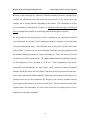
9.6 Appendix F - Interactions of RF Energy and Biological
Tissues (DL)
This section will give a brief introduction into the theory of boundary conditions
of a traveling RF wave hitting the various tissue types of the body. Also explored are the
permeability and conductivity of said tissues.
When thinking about interactions between electromagnetic waves and biological
tissue, the concepts are no different than considering the interactions between a wave of
any frequency and a boundary and material of any conductivity, permeability, and
permittivity. In all types of body tissue, magnetic permeability is very closely equal to
µo, or the permeability of free space. This fact makes most calculations involving body
tissues simpler. The more important concepts to consider at the frequencies the prototype
will operate at (900MHz and 2.4GHz) are the reflectivity coefficients and skin depth of
penetration, because from these, energy absorption and the distribution of energy can be
derived. While the specifics of energy distribution inside a tissue is rather complex and
beyond the scope of our research, we are still interested in net energy (and thus power)
absorption to determine if our power output will be within OSHA-defined limits.
It is worthwhile to note that for the antennas to be used, and at the frequencies
transmitted, all occurrences will happen in the far-field region of the antenna. The farfield region is defined as the region of space, a minimum distance l from the emitting
antenna to infinite, that the transmitted energy waves can be seen as a predominantly
plane-wave character (electric vector E is perpendicular to the H-field vector) [17]. The
53
Doppler Radar for Biomedical Measurements
Ball, Lamppa, Marrero, Selina, Sugimoto
region of operation for our device, 0.5 m at the closest to 2m, nearly assures operation in
the far-field region of the antennas, which is defined by the equation [17]:
Where D is the larger dimension of the antenna and with wavelength λ as defined
by [15]:
Wavelengths λ for the frequencies of our devices are 33 cm, for 900MHz, and 12.5 cm,
for 2.4GHz. These yield far-field regions beginning at 27 cm (D = 20.32 cm) and 16 cm
(D = 10.8 cm), respectively. The fact that the prototypes will be operating in the far-field
region assures simpler power calculations and considerations: the power density travels
as one over the square of the distance traveled in the far-region (as opposed to having to
calculate the more complex oscillations that characterize power transmission in the near
field) [17].
When the near-planar wave of energy hits the body tissue, the system acts as a
typical wave hitting a boundary with different characteristics than the current medium. In
this case, the wave traveling in free space (air) contacts the skin of the patient. As with
any such interaction, part the wave is reflected back to the source while the remnant is
transmitted into the skin. The reflection coefficient that defines what is reflected back is
dependent upon the frequency of the wave, the permeability, conductivity, and
permittivity of both sides of the boundary. Its value is determined by using a ratio of the
54
Doppler Radar for Biomedical Measurements
Ball, Lamppa, Marrero, Selina, Sugimoto
pre- and post-boundary impedances defined by the aforementioned characteristics. A
discussion of the coefficient can be found in the CRC Handbook of Biological Effects of
Electromagnetic Fields [17], pages 14-15. The governing equation is found below:
Γ=
η 2 − η1
η 2 + η1
Where Γ is the reflection coefficient and η is the wave impedance of medium 1
and 2.
Continuing the discussion of the air-to-skin transmission, the transmitted wave
inside the boundary will continue to penetrate the body, but it will attenuate at an
exponential rate, dependent on the skin depth of the material17. The skin depth δ is also a
function dependent on the medium’s permittivity, permeability, and conductivity, as well
as the wave’s frequency.
Refer to the CRC Handbook of Biological Effects of
Electromagnetic Fields [17] for a discussion and the governing equations for transmission
attenuation and skin depth calculation. Here is a table of calculated skin depths for
various tissues at various frequencies. Frequencies of interest are the 915 MHz and the
2450MHz rows. Follows is the equation that governs skin depth for all materials:
1
δ=
ω
µε
2
55
−1+ 1+
σ
ωε
Doppler Radar for Biomedical Measurements
Ball, Lamppa, Marrero, Selina, Sugimoto
Figure 17 - Skin Depth as a Function of Frequency
The human body of course does not consist of a homogenous material (single
tissue) with a single boundary at the skin. Each tissue has its own permittivity and
conductivity characteristics. The biology of this is interesting, but only worth a cursory
mention; factors such as the average water content of a tissue, cell size and shape, intraand extra-cellular ion concentration, and plasma membrane structure play a part in
defining the cell’s characteristics. A table of the conductivities and permittivities of the
various tissues can be found in Appendix E. These properties are noticeably different
from tissue to tissue and warrant calculations for each transition.
56
Doppler Radar for Biomedical Measurements
Ball, Lamppa, Marrero, Selina, Sugimoto
Because of this heterogeneity, numerous different boundaries must be considered; for
example, the path between the skin and the heart has layers of fat, muscle, bone and
cartilage, all in varying amounts, depending on the patient. The calculations to do this
are too elaborate to examine here; Chapter 6 in Engineering Electromagnetic Fields and
Waves contains the procedure for considering multiple heterogeneous regions.
At the frequencies that the prototypes will be operating at, the penetration (and thus
power dispersal) the majority of the transmitted energy is absorbed as the attenuating
wave passes through the body. After this point, most of the power will have either been
reflected back or absorbed by the tissues through which the wave has propagated (with
the minimal remaining amounts of energy continuing on). Thus, the tissues of concern
are the focus of safety considerations. The OSHA standard limit for continuous exposure
for the frequencies of our operation is 10 W/cm2. Other organizations also release
comparable recommendations for legal limits; ANSI (American National Standards
Institute) and IEEE release their own limits, with the former being stricter than the latter,
whose values parallel the OSHA standards. While the power output for the range of our
prototypes have not yet been measured, the designer of the circuitry estimates that the
power output of the antennas are well below this limit. This is beneficial, because if the
resulting data is not discernable, we will be able to increase our output power to receive
signals back with higher amplitude.
57
Doppler Radar for Biomedical Measurements
Ball, Lamppa, Marrero, Selina, Sugimoto
9.7 Appendix G - Breakdown of the Major Radar Front-End
Components (KS)
Mixer
There are two signals that are compared by the mixer. One is from the local oscillator
(the VCO) and is referred to as LO. The second is the reflected signal that comes from
the RF antenna and is appropriately referred to as the RF. If we represent LO as cos ω1t
and RF as cos ω 2 t , we can evaluate their relationship in the mixer as
follows: (cos ω1t )(cos ω 2t ).
A circuit diagram demonstrating how this relationship is achieved is shown below:
Figure 18 - LO Circuit Equivalence
As you can see from the circuit, a certain level of power is required on the LO input to
properly driver the mixer diodes. LO power level has to be sufficient in order to turn on
the diode in the saturation mode. The LO power level must also be much larger than the
RF power level in order to prevent load distortion. The LO drive level plays a critical
role in determining the IP3, 1 dB Compression Point and Dynamic Range of a mixer. For
higher performance applications, Pulsar recommends as a minimum the use of a +17
dBm level mixer.
58
Doppler Radar for Biomedical Measurements
Ball, Lamppa, Marrero, Selina, Sugimoto
Voltage Control Oscillator
A fundamental oscillator circuit is shown in Figure 19.
Figure 19 - Fundamental Oscillator Circuit Representation
In order to oscillate, the total phase shift of this closed loop has to be 360 degrees and the
gain must be one:
Vo
A
=
Vi (1 − βA)
In our project, we used a 2.4GHz oscillator.
Figure 20 - VCO Representation
Figure 20 is the common configuration of the crystal oscillator. Most oscillators operate
at “parallel resonance” where the reactance vs. frequency slope,
dx
, is inversely
df
proportional to C1, the motional capacitance of the crystal unit. The principal
mechanism of the voltage-controlled oscillator is that the circuit is only marginally stable.
Thus the output of the system oscillates at the constant amplitude and frequency.
59
Doppler Radar for Biomedical Measurements
Ball, Lamppa, Marrero, Selina, Sugimoto
9.8 Appendix H – Radar Evaluation and Design (KS)
In this section we will introduce some concepts that would have been necessary in the
full design of a radar system. The design flow and power are discussed in the flow chart
below:
1. Determination of adequate signal and frequency which can provide sufficient
information of the target.
Measurement
Doppler Shift
Phase Shift
Detection
Signal to Noise Ratio (S/N)
2. Power calculation at the transmitter, receiver, and target.
Received Power Density at the Target
Power Absorbed by the Target
Reflectivity
Radar Cross Section
Safety of Radiation
ANSI
OSHI
FCC
Phase Noise
Impedance Matching
60
Doppler Radar for Biomedical Measurements
Ball, Lamppa, Marrero, Selina, Sugimoto
3. According to the information above, choose antenna types and specifications.
Antenna types
Antenna power and gain
Antenna dimension
Based on the desired power density, the antenna specifications such as antenna type, gain,
dimensions and power can be determined.
4. Fundamental RF circuit design and analysis
Component types
Tubes
Semiconductors
Three primary components
VCO
Mixer
Filter
Determination of adequate signal and frequency
Higher frequency operation (shorter wavelength) can make the antenna size smaller. It
can also increase the range of the unit and make any phase changes more distinguishable.
When designing a Doppler radar, we need to determine if the target moves fast enough to
give us a Doppler shift. If not, a phase detector type application is the alternative. Actual
received power at the antenna is obtained by the following equation:
61
Doppler Radar for Biomedical Measurements
Ball, Lamppa, Marrero, Selina, Sugimoto
Pt Gt Gr λ2
Pr =
σ
(4π ) 3 R 4
Signal to Noise Ratio (S/N)
The signal-to-noise ratio needs to be considered at this stage. The S/N ratio shows can be
used to determine how difficult it will be to extract the desired signal from the noise
present in the system. The noise is defined as N=kTB, where k is the Boltzmann’s
constant (-228.6dBW), T is temperature, and B is the noise bandwidth.
Combining two equations gives us the S/N ratio expressed as follows:
P G G λ2
S
= t 3t 4r
σ
N (4π ) R kTB
A signal-to-noise ratio of greater than 10dB is the typical way to set up these system’s
efficiency.
Power calculation at the transmitter, receiver, and target
The power density at the target is obtained from following equation:
Pt Gt Gr λ2
Pr =
(4π ) 2 R 2
Pt = -20dB(10dBm), Gr=Gt=8dB(8dBi),
The parameters are divided to the numerator and denominator. After converted into dB,
the parameters which are listed in the numerator are simply added and the parameters on
the denominator are subtracted. Knowing this figure, one can adjust the power
62
Doppler Radar for Biomedical Measurements
Ball, Lamppa, Marrero, Selina, Sugimoto
transmitted and received to determine if sufficient signal strength is available at the RF
input of the mixer. This is discussed in greater detail in Appendix G.
Phase Noise
In order to obtain the highest functionality of the system, typical signal distortion such as
phase noise or “jitter” needs to be considered. Let say that a perfect VCO would produce
an ideal sine wave:
V (t ) = A sin(ωt )
However, there is inherently some noise introduced to the signal. This can be
represented by fluctuations in the amplitude of the signal and by fluctuations in the signal
phase. We can represent the noisy oscillator signal as:
V (t ) = ( A + a (t )) sin(2πf o t + φ (t ))
where a(t) represents the amplitude noise and Φ(t) represents the phase noise.
Amplitude noise can be removed to some degree by using automatic level control
(ALC) systems. However, phase noise is another matter. It is very difficult to remove.
The equation can be rewritten ignoring amplitude noise:
V (t ) = A sin( 2πf o t + φ (t ))
The picture below shows the effect of Φ(t).
63
Doppler Radar for Biomedical Measurements
Ball, Lamppa, Marrero, Selina, Sugimoto
Figure 21 - Phase Noise Diagram
Phase noise is a serious source of interference, such as “timing error” in the RF design.
Especially in our system, which obtains information from the phase shift measurement.
“Minute amounts of phase noise on a transmitter signal can result in the
transmitter causing significant interference to other services, whereas minute amounts of
phase noise on a receiver local oscillator can severely reduce the receiver selectivity or
cause other undesirable effects.” [26] Minimizing phase noise is one of most important
factors in the selection of a VCO and is frequently a selling point in the VCO spec sheet.
Impedance Matching
Impedance matching is another important aspect of RF circuit design. Matching the
source impedance and the load impedance produces maximum output power and avoids
creating standing waves. A mismatch caused by these can result in interference when
they add or subtract signals on the transmission line. This is avoided by careful design
64
Doppler Radar for Biomedical Measurements
Ball, Lamppa, Marrero, Selina, Sugimoto
during the board etching process. Our boards were professionally designed and etched by
MiniCircuits.
Antenna Types
There are many different types of antennas: a few examples are helix, yagi, and patch
antennas. Patch antennas are employed in our project because of their small size, but yagi
antennas were very appealing due to their increased directionality.
Antenna Dimension
It is appropriate to compare the antenna’s dimensions with the size of the wavelength
instead of just evaluating its physical size. For instance, a 30m high AM antenna is small
in terms of its wavelength, which is 300m. One advantage of using microwave frequency
bands is that the wavelengths (and thus the antennas) are rather small. In our project, the
antenna has a physical size of 9.9cm x 10.7cm. This is efficient when we consider the
wavelength, which is 12.5cm.
Antenna gain can be obtained by the following equation:
G = ηA
4πA
λ2
= ηA
πD
λ
2
Antenna gain is proportionally related to the area (A) of the antenna and inversely
proportional to the wavelength. For this project, one reason why the 2.4GHz band was
selected was the smaller antenna size. From the above equation above, the antenna
efficiency, η A also can be determined as follows:
ηA =
Gt λ 2
= 0.7311
4πA
65
Doppler Radar for Biomedical Measurements
9.9
Ball, Lamppa, Marrero, Selina, Sugimoto
Digital Appendices
The following files are available on the CD-ROM:
Executable File
Source Code
Sample Data Sets
User Manual
66