1
Connecting TCAD To Tapeout
A Journal for Circuit Simulation and SPICE Modeling Engineers
HiSIM Methodology for the Parameter Extraction
in Accordance with the Model Derivation
I. Introduction
voltage parameter extraction comes at the very first of
the extraction procedures. In contrast, HiSIM calculates
the surface potential by applying Poisson equation to the
channel region and the potentials are used for the drain
current computation with no explicit threshold voltage
parameter. The followings are the HiSIM formulas of the
drain current with the surface potentials.
HiSIM (Hiroshima university STARC IGFET Model)
is one of the surface potential based Spice models [1],
[2] and pioneered the iterative approach to obtain the
surface potential applicable in compact models. The
model aims for MOSFET technology of 100 nm or below.
The parameter extraction procedure was introduced
first by the model developers: Semiconductor Technology Academic Research Center (STARC) [3], [4]. Silvaco
UTMOST-III introduced the first version of the local
optimization strategies for HiSIM-1.1 in 2002 [5]. Since
then, the parameter extraction methodology has been
reviewed thoroughly. This article is meant to provide
significant aspects on the HiSIM version 1.2 parameter
extraction for UTMOST-III users.
(23)
Since the surface potential is obtained by solving Poisson
equation, and the geometric effects are directly related to
the electric field calculated from the potential, establishing the HiSIM model parameter extraction methodology
forces traditional SPICE modeling engineers to refresh
their understanding of device physics. Moreover, making the HiSIM model to be scalable over the wide geometric region challenges the experienced manner of this
tradition. In this paper, each step of the developed HiSIM
model parameter extraction is discussed from the model
derivation point. The model parameters are symbolized
with the capital, bold and italic letters. Also, the HiSIM1.2 equations and the numbers used herein are based on
HiSIM1.2.0 user’s manual [3]. The detailed UTMOST-III
local optimization strategies with the practical application results will be covered in a future edition of simulation standard issued by Silvaco International.
(11)
(12)
(13)
(73)
Continued on page 2 ...
INSIDE
II. HiSIM Methodology
Behavioral Modeling of PLL Using Verilog-A ........... 4
Accounting for Shallow-Trench-Isolation (STI)
Effects in BSIM4 and HiSIM MOSFET Models .... 7
A. Substrate Model Parameters
MOSFET threshold voltage parameter (Vth) is very
popular in MOSFET Spice models such as in the Level-1,
2, 3 and in the UC Berkeley BSIM3 models. The threshold
Volume 13, Number 7, July 2003
July 2003
Calendar of Events..................................................... 10
Hints, Tips, and Solutions ......................................... 11
Page 1
The Simulation Standard
Vth represents the threshold voltage shifts referring to
the long channel device including the short channel
(∆Vth,SC), the reverse short channel (Vth,R and Vth,P), and
the reduced channel width (Vth,W) effects. Most of them
are related to the electric field gradients for the lateral
direction.
(52)
(53)
Therefore, the substrate parameters such as the substrate
impurity concentration (NSUBC), the flat-band voltage
(VFBC), the maximum pocket concentration (NSUBP),
and the pocket penetration length (LP) are to be determined first. At the same time, the oxide thickness ((TOX) is
also to be fixed as the source of the vertical electric field.
(39)
Effective impurity concentration used in the HiSIM
equation is the averaged value using NSUBC, NSUBP,
and LP parameters (eq.39). The eq.39 was supposed to
limit the LP value less than the Leff value. However, the
formula enables it become larger than the Leff. There is
no structural constraint, which was found through the
trial parameter extraction applied for 90 nm technology
[6]. For long and wide channel devices, the NSUBP and
LP have less influence and the initial value determination appears to be arbitrary. But, the LP must be defined
and the remaining substrate parameters should be
extracted under the fixed value at the first step of the
extraction. The reasonable approach to define the LP is
under investigation.
In addition, the surface roughness effect might be indistinguishable from the HiSIM pocket resistance parameter effect. The Ids degradation at the high Vgs could be
expressed only with the surface roughness parameter.
However, it might be an overestimation of the decreasing mobility. And the short channel length devices might
show the smaller Ids current for the target curves.
C. Geometric Effects: Reverse Short Channel Effect
HiSIM geometric effects toward the MOS channel length
such as the reverse short channel (RSC) and the standard
short channel (SC) effects need the careful approach. The
HiSIM RSC expression is based on the impurity inhomogeneity in the lateral direction and the lateral electric
field strength is modified as following.
The TOX requires a capacitance voltage curve (CGG)
for the determination. The substrate related parameters
could be fixed using Ids versus Vgs curve for the large
geometry transistor. Also, the capacitance curve could
be appropriate for the initial value findings. Naturally,
gate current contribution must be considered for very
thin gate oxide devices.
(35)
(36)
(37)
With those initial values, the sub-threshold drain current
region is used for the substrate parameter optimization.
Since HiSIM has no body effect coefficient parameters
like in the previous generation models, the substrate
parameter determination at the very first stage almost
destines the body bias behavior of the HiSIM model.
(38)
The four model parameters such as PARL1, SCP1, SCP2,
and SCP3 in addition to the substrate related parameters
(NSUBC,
NSUBC, NSUBP
NSUBP, and LP) are included in the equation.
(39)
B. Carrier Mobility: Low Field Mobility
HiSIM low field mobility model follows the mobility
universality [7]. Three scattering mechanisms such as
Coulomb, phonon, and surface roughness effects are
taken into account.
(50)
(51)
The Simulation Standard
The gate bias region of Ids versus Vgs should be properly
selected with this mobility universality in mind for the
parameters (MUECB0, MUECB1, MUEPH1, MUESR1)
using the wide channel width and the long channel
length (large) device. Although the target I-V curve for
the large device is easily expressed with the rough bias
selections, the scalable model would become difficult to
be achieved. Some parameters are related with the electric field component. The low field mobility characterization with split C-V method might provide an insight for
the bias selection.
Page 2
The NSUBP under the fixed LP should be mainly used
to express a shift of Ids versus Vgs curve to the larger Vgs
(Vth roll-up) of the RSC devices. And it should be modified carefully to have the small effect on the SC device
curves. Too much change on the SC device characteristics at this step means the shift of Ids versus Vgs toward
the smaller Vgs (Vth roll-off) couldn’t be expressed later
with any effort. It means the pre-defined LP is too small
July 2003
to assign the larger contribution to the NSUBP for the
averaged Nsub. The LP must be redefined, other substrate parameters also must be extracted according to the
previous description. So that the NSUBP value could become reasonable compared to the NSUBC, and the RSC
effect could be expressed clearly [8].
(61)
(62)
One of remaining four parameters, PARL1, is fixed to
unity. SCP1 appears to be used for the slight tuning of
the RSC effect expression. And SCP3 could be used to
modify the body bias effect for the RSC devices. Finally,
SCP2 which relates the RSC effect with the drain bias
needs to be optimized for Ids versus Vgs under the saturation condition.
The HiSIM maximum velocity ((VMAX ) modulation
adopts a nonlinear expression with two model parameters which are related to the channel length. The lateral electric field is also the function of channel length.
Therefore, the high field mobility dependency on the
channel length could become complex and hard to be
predicted. Therefore, tuning over the wide range of the
channel length would be the most critical step to obtain
the scalable model parameters over the channel length.
D. Geometric Effects: Standard Short Channel Effect
The standard short channel effect is expressed with the
similar formula for the reverse short channel effect.
(28)
(29)
(30)
(31)
In order to trace the drain bias influence, Ids versus Vgs
curves under the various drain voltages appear to be suitable as the target characteristics for the parameter optimization. Whether the equation could be capable of depicting the scalability for 100 nm below technology, or not,
requires the verification with various technology devices.
F. Geometric Effects: Narrow Width Effect
HiSIM-1.2 narrow width effect description which takes
the shallow trench isolation (STI) technology into account looks simple, and has waited for the validation
using the actual and practical devices.
However, such four parameters as PARL2, SC1, SC2, and
SC3 should be optimized carefully to obtain the standard
short channel (SC) effect. PARL2 has the length dimension, modifies the effective channel length used in the SC
effect equation and shows much influence on the effect.
SC1 parameter has also the great effect to pull the overshot Ids versus Vgs curves resulted by the RSC expression
toward the Vth roll-off (SC effect) direction. Also, SC2
influences the higher drain bias region of Ids versus Vgs
curves, and expresses the SC effect dependency on the
drain bias. The extraction of the standard short channel
parameters requires the software optimizer to be used
with much care. Especially, both the SC1 and SC2 values
spread widely between 0 and 200 depending on the device characteristics of RSC and SC effects.
(71)
(72)
A trial report on this methodology reveals the effectiveness of HiSIM approach [6].
G. Geometric Effects: Wide Width Effect
The second STI effect expression in HiSIM-1.2 is the mobility reduction assuming the STI induced mechanical
stress. The wider device is supposed to suffer the mobility degradation.
E. Carrier Mobility: High Field Mobility
Now that such parameters as the substrate, the low field
mobility and the RSC and SC effect parameters are fixed
using the Ids versus Vgs at the low Vds, HiSIM high field
mobility parameters should be extracted. The HiSIM
high field mobility is obtained by modifying the low
field component with the lateral electric field in association with the modulated maximum velocity parameter.
(72)
H. Geometric Effects: Hump in Sub-Threshold Current
(60)
Another STI induced effect in HiSIM-1.2 is the drain
current hump in the sub-threshold region. As far as the
parameter extraction for the varied channel length is
concerned, further validation seems to be required.
Continued on page 6 ...
July 2003
Page 3
The Simulation Standard
Behavioral Modeling of PLL Using Verilog-A
Introduction
In this article, we describe practical behavioral modeling
for highly non-linear circuits using Verilog-A, which is
analog extension of Verilog-AMS. At first, we describe
behavioral modeling techniques for phase/frequency
detectors (PFD) and voltage-controlled oscillators (VCO)
those are essential part of phase-locked loop systems
shown in Figure.1. Model parameter extraction techniques are described and demonstrated later. Finally,
these models are simulated with SmartSpice and verified
against the results of transistor circuit simulations.
Phase/
Frequency
Detector
feedback
clock
Loop
Filter
DOWN Charge Pump
Voltage
Controlled
Oscillator
Divider
/4
VCO in
Figure 1. PLL Block Diagram.
REF clock occurs before the rising edge of FB clock, the
module activate UP signal and then forces the VCO to
increase the oscillation frequency. In the reverse case,
the module activate DOWN signal and forces the VCO to
decrease the frequency. Note that UP and DOWN signal
are active-low and active-high respectively.
Phase Detector (PD)
A well-known sequential-logic PFD shown in Figure.2(a)
is used for phase/frequency detection circuit. This PFD
produces UP and DOWN signals depending on the
phase difference between reference clock and feedback
clock (Figure.2(b)).
List 1. Behavioral representation of PFD in Verilog-A
module pll_pd (ref_clk, fb_clk, up_out, down_out);
Phase Detector (PD)
inout ref_clk, fb_clk, up_out, down_out;
A well-known sequential-logic PFD shown in Figure.2(a)
is used for phase/frequency detection circuit. This PFD
produces UP and DOWN signals depending on the
phase difference between reference clock and feedback
clock (Figure.2(b)).
electrical ref_clk, fb_clk, up_out, down_out;
parameter real vdd=3.3,
ttol=10f,
ttime=0.2n ;
The behavioral model of PFD can be represented as
shown in List.1. This module monitors the phase difference between the clocks. When the rising edge of
REF
UP
reference
clock
integer state;
real
// state=1 for down, -1 for up
td_up, td_down ;
UP
DOWN
FB
(a)
Figure 2a. PFD circuit.
The Simulation Standard
Figure 2b. Basic operation.
Page 4
July 2003
Voltage Controlled Oscillator (VCO)
analog begin
@(cross( V(ref_clk) - vdd/2 , 1 , ttol )) begin
An ideal voltage-controlled oscillator generates a periodic output signal whose frequency is a linear function
of control voltage. The output frequency fout can be
expressted as;
state = state - 1;
if(V(up_out)>vdd/2) td_up=480p; else td_up=1005p;
if(V(down_out)<vdd/2) td_down=480p; else td_down=1090p;
end
fout = fnom + gain*Vcont
@(cross( V(fb_clk) - vdd/2 , 1 , ttol )) begin
where fnom is a nominal(or free running) frequency,
gain is the gain of VCO in Hz/V, and Vcont is a control
voltage supplied from charge pump. Since phase is the
time-integral of frequency, the sinusoidal output of VCO
can be expressed as;
state = state + 1;
if(V(up_out)>vdd/2) td_up=480p; else td_up=1005p;
if(V(down_out)<vdd/2) td_down=480p; else td down=1090p;
end
Vout(t) = A*sin(2*phi*integral(out) ) + Voffset
where A is a amplitude of sinusoidal and Voffset is an
output offset voltage.
if ( state > 1 ) state = 1 ;
if ( state < -1 ) state = -1;
With based on the above principle, behavioral model of
VCO can be represented as shown in List.2.
V(down_out) <+ transition( (state + 1)/2*vdd , td_down , ttime );
V(up_out) <+ transition( (state - 1)/2*vdd+vdd , td_up , ttime );
end
List 2. Behavioral representation of VCO in Verilog-A
endmodule
module pll_vco ( in, out ) ;
In this module, we use td_up and td_down variables to
define delay time of input-to-UP and input-to-DOWN
respectively. Since delay time of rise transition is different from fall transition, different values should be assigned to these variables depending on output transition
direction. The following codes used in the module allow
designers to define different delay time for rise and fall
transition independently.
inout
in, out ;
electrical in, out ;
parameter real vdd = 3.3, // operational voltage
amp = vdd/2,
// amplitude of vout
offset = vdd/2, // offset of vout
if(V(up_out)>vdd/2) td_up=480p; else td_up=1005p;
gain = 540e6,
// gain [Hz/V]
vnom = 1.27,
// nominal vin
fnom = 400e6; // frequency at vnom
if(V(down_out)<vdd/2) td_down=480p; else td_down=1090p;
real
The optimal value of variables can be obtained from
transistor level simulation shown in Figure.3 (a) and (b).
From these plots, we can obtain the optimal value of td_
up=480ps when rising and td_up=1005ps when falling,
and td_down=480ps when rising and td_down=1090ps
when falling. By using these optimal values, we can see
good agreement in the output waveforms of both transistor level and Verilog-A simulations.
freq ;
analog begin
freq = fnom + gain*(V(in) - vnom) ;
V(out) <+ amp*sin(2*`M_PI*idt(freq)) + offset ;
end
endmodule
Figure 3. Simulation results of PFD. Shown are (a) UP waveforms, and (b) DOWN waveforms.
July 2003
Page 5
The Simulation Standard
Note that, Vcont is replaced by V(in)-vnom in the module description.
The module parameters fnom is the nominal frequency
and is defined in design specification. The ‘offset’ may
be defined as half of VDD. The vnom and gain should be
extracted from transistor level simulation. Figure.4 shows
the transistor level simulation result of VCO frequency
respect to control voltage. vnom can be found by measuring control voltage at which VCO frequency is equal to
400MHz, and gain can be obtained by calculating the gradient of the curve at Vcont=vnom. In this example, we obtained vnom=1.27v and gain=540MHz/V from the plot.
Verilog-A simulation result is also displayed in Figure.4.
Since we assume the VCO gain is a linear function of
control voltage, there’s a discrepancy in low and high
regime of Vcont. However, you can overcome this issue
by adapting non-linear function for gain expression.
Figure 4. Simulation results of VCO.
Conclusion
By using behavioral modeling technique, and a mixed
signal simulation with SmartSpice, PLL system can be
efficiently simulated with good accuracy and reasonable
run-time cost. The module characteristic can be parameterized in behavioral representation, and the parameters
can be easily extracted from the transistor level simulation. A designer would thus start the design process by
using an all behavioral model of PLL and focusing on
optimizing module parameters. Once enough performance is obtained, the modules can be widely used for
various subsystems and in a mixed signal simulations in
future designs.
...continued from page 3
V. Summary
References
The methodology on HiSIM-1.2 model parameter
extraction was discussed from the model derivation
point. HiSIM-1.2 incorporates other effects such as
Poly-Depletion, Quantumn-Mechanical, ChannelLength Modulation, etc.. The readers of interest should
refer to HiSIM-1.2.0 user’s manual [3]. The practical
procedure was applied to the actual N-channel MOS
devices and the HiSIM-1.2 model parameter set was
obtained. The simulated result demonstrated the geometrical scalability down to 100 nm from 10 um channel length with no binning at all. The UTMOST-III local optimization strategies with the applied result will
appear on a future issue of Simulation Standard from
Silvaco International.
[1]
M. Miura-Mattausch et al., “HiSIM: A MOSFET Model for Circuit
Simulation Connecting Circuit Performance with Technology,”
Tech. Digest of IEDM, pp. 109 -112, 2002
[2]
http://www.semiconductor.philips.com/Philips_Models/mos_models
[3] “HiSIM1.2.0 User’s manual”,Semiconductor Technology Academic
Research Center (STARC), 2003 http://www.starc.or.jp/kaihatu/
pdgr/hisim/index.html
[4] K. Tokumasu et al., “Parameter Extraction of MOSFET Model HiSIM”, IPSJ DA Symposium (in Japanese), A10-2, 2002
[5] “HiSIM version 1.1 Model Released in UTMOST-III”, Silvaco International, Simulation Standard, Volume 12, Number 7, July 2002
http://www.silvaco.com
[6] Y. Iino, “A Trial Report: HiSIM-1.2 Parameter Extraction for 90 nm
Technology”, 2004 Workshop on Compact Modeling, WCM 2004,
in association with 2004 NSTI Nanotechnology Conference and
Trade Show (http://www.nsti.org)
[7] A. Toriumi et al., “On the Universality of Inversion layer mobility,”
Tech. Digest of IEDM, pp. 398- 401, 1988 Private communication
with the HiSIM developer
The Simulation Standard
Page 6
July 2003
Accounting for Shallow-Trench-Isolation (STI) Effects in
BSIM4 and HiSIM MOSFET Models
1. Introduction
Semiconductor devices are continuously improved with regard to intrinsic characteristics,
as well as reduced geometries. Among all requirements, there is a need for an efficient device isolation technique as CMOS technologies
are scaled down below the 0.25µm generation.
Shallow Trench Isolation (STI) has become an
essential isolation scheme as a replacement for
LOCal Oxydation of Silicon (LOCOS). It allows
reaching a higher packing density, tighter design
rules, lower parasitics and higher yields. However, the basic STI process sequence involves
Figure 1. Mechanical stress induced by STI process.
several sources of mechanical strain, which can
significantly increase the stress levels in the enclosed
silicon area (Figure 1). It was shown that this stress in
turn influences junction leakage but also MOS electrical
characteristics. There are several ways to account for the
effect of STI-induced stress in standard compact models.
The purpose of this article is to present two different approaches developed by the universities of Berkeley and
Hiroshima. In both cases, new equations were derived
and new parameters have been introduced in the latest
versions of BSIM4 and HiSIM compact models. These new
versions are currently supported by Silvaco SmartSpice/
UTMOST softwares.
The edge of the trench has an influence on the electric
field. The impurity concentration and the oxyde thickness are different from those at the middle of the width.
Therefore, a modified surface potential is computed.
Since the threshold voltage for the corresponding leakage current is different from the threshold voltage of the
main current, the STI effects can be observed only in the
sub-threshold region.
The local modified surface potential is computed using
the expression shown in equation 1.
HiSIM is a MOSFET model developped by Hiroshima
University, started in 2001. The equations for the STI effect
were added in version 1.1 and account for two major STI
effects experimentally observed on I-V characteristics:
These equations are based on the assumption that the
current in the subthreshold region is mainly due to diffusion. The carrier concentration, QN,STI, is calculated
analytically using the Poisson equation, with a dedicated
substrate impurity concentration NSTI. The WVTHSC parameter is used to discriminate the short-channel threshold characteristics of the edge from the intrinsic part.
•
a “double hump” in the Id/Vg characteristic (subthreshold region),
The final equation is shown in equation 2.
•
a lower threshold voltage value.
2. HiSIM STI Model Equations
The WSTI parameter represents the width of the
high-field region.
An example of the I-V characteristics
is shown on Figure 2. It is important to
note that unrealistic parameter values
are used to make the “double hump”
and the lower threshold voltage visible.
For most practical situations, the effect
on I-V characteristic is not so important
and may be negligeable with optimized
STI processes.
Equation 1.
Equation 2.
July 2003
Page 7
The Simulation Standard
Figure 2. STI-induced stress effect on Id-Vg characteristics.
Figure 3. Irregualr LOD device geometry parameters.
3. BSIM4 STI Model Equations
The approach chosen by the University of Berkeley is based
on the observation that the mechanical stress induced by
STI makes MOSFET performance depend on the active
area size, as well as the location of the device in the active
area. The effect of stress on mobility and saturation velocity
was experimentally demonstrated. A phenomenological
model was derived and introduced in BSIM4v3.0 to consider the influence of stress on mobility, velocity saturation,
threshold voltage, body effect and DIBL effect.
•
The TSMC model was developed to account for devices
with irregular oxide definition (Figure 3). Berkeley models must be used for multi-finger devices (Figure 4). If
only SA (or SA1) and SB (or SB1) are specified with NF=1,
STIMOD=2 and STIMOD=3 models are equivalent.
In the Silvaco implementation of BSIM4, several stress effect
models can be invoked by specifying the model parameter
STIMOD. This selector was not supported in the original
Berkeley release of BSIM4v3.0. As STI effect is turned off by
default, it is supported for all versions of BSIM4.
•
STIMOD=3 (Berkeley model for multi-finger devices)
This model was introduced by Berkeley in the final
release of BSIM4.3.0 of May 9th 2003. It considers the
influence of stress on mobility, velocity saturation,
threshold voltage, body effect and DIBL effect by
modifying the parameters shown in Equation 5.
STIMOD=0
Stress effect turned off.
•
STIMOD=1 (Berkeley model introduced in
BSIM4.3.0 beta of December 2002) If instance
parameters SA, SB are set to positive values
with NF=1 or if SA, SB, SD are all set to positive values with NF>1 and the model parameter SK0 is also set to a positive value, the mobility U0(T)and the carrier velocity VSAT(T)
account for changes due to stress effect and
are expressed as shown in Equation 3.
•
STIMOD=2 (TSMC model for irregular LOD
devices) This model corresponds to the Berkeley model (STIMOD=3) with different expressions for the intermediate variables Inv_sa Equation 3.
and Inv_sb. These latter ones are computed as
functions of instance parameters SA1...SA10,
SB1...SB10 and SW1...SW10 to account for irregular LOD devices. NF must be unspecified
or set to 1 to allow stress effect computation if
STIMOD=2 is invoked. (Equation 4.)
Equation 4.
The Simulation Standard
Page 8
July 2003
Equation 5.
4. Conclusion
BSIM4 and HiSIM offer two different ways
to account for the same physical phenomenom. The HiSIM model is physically-based
but requires the computation of extra biasdependent equations, which may be timeconsuming when running large circuits. The
Berkeley model is phenomenological and has
no impact on simulation time because only
some parameters are modified during preprocessing calculations (temperature- and
geometry-dependent parameters). The accuracy of both models may vary significantly
with STI processes.
Figure 4. Multi-fingers device geometry parameters.
July 2003
Page 9
The Simulation Standard
Calendar of Events
July
1
2
3
4
5
6
7
8
9
10
11
12
13
14
15
16
17
18
19
20
21
22
23
24
25
26
27
28
30
AM-LCD - Kogakuin Unv, Tokyo
AM-LCD - Kogakuin Unv, Tokyo
AM-LCD - Kogakuin Unv, Tokyo
IMFED - Osaka, Japan
IMFED - Osaka, Japan
IMFED - Osaka, Japan
NSREC - Monterey, CA
NSREC - Monterey, CA
NSREC - Monterey, CA
NSREC - Monterey, CA
NSREC - Monterey, CA
August
1
2
3
4
5
6
7
8
9
10
11
12
13
14
15
16
17
18
19
20
21
22
23
24
25 ISLPED - Soeul, Korea
ISCS - San Diego, CA
26 ISLPED - Soeul, Korea
ISCS - San Diego, CA
27 ISLPED - Soeul, Korea
ISCS - San Diego, CA
28
29
30
31
Bulletin Board
Silvaco Donates Software to
University if Washington
Silvaco donated $2.4 million of
software to the University of Washington College of Engineering to create an intellectual hub for advanced
technology computer aided design
(TCAD) research and development.
The donated software simulates the
behavior of semiconductor processes
and devices using 3D field solvers
to solve complex physics equations.
The college of engineering faculty
and graduate students will use this
software to model reliability and
performance of semiconductors as
part of a joint development project
between the University and Silvaco
launched on May 19, 2003.
See Silvaco at NSREC
The IEEE Nuclear and Space Radiation Effects Conference (NSREC)
presents the latest techniques for
enhancing the performance of microelectronic devices and circuits that
are used in radiation environments.
If you would like more information or to register for one of our our workshops, please check our web site at http://www.silvaco.com
The Simulation Standard, circulation 18,000 Vol. 13, No. 7, July 2003 is copyrighted by Silvaco International. If you, or someone you know wants a subscription to
this free publication, please call (408) 567-1000 (USA), (44) (1483) 401-800 (UK), (81)(45) 820-3000 (Japan), or your nearest Silvaco distributor.
Simulation Standard, TCAD Driven CAD, Virtual Wafer Fab, Analog Alliance, Legacy, ATHENA, ATLAS, MERCURY, VICTORY, VYPER, ANALOG EXPRESS,
RESILIENCE, DISCOVERY, CELEBRITY, Manufacturing Tools, Automation Tools, Interactive Tools, TonyPlot, TonyPlot3D, DeckBuild, DevEdit, DevEdit3D,
Interpreter, ATHENA Interpreter, ATLAS Interpreter, Circuit Optimizer, MaskViews, PSTATS, SSuprem3, SSuprem4, Elite, Optolith, Flash, Silicides, MC Depo/
Etch, MC Implant, S-Pisces, Blaze/Blaze3D, Device3D, TFT2D/3D, Ferro, SiGe, SiC, Laser, VCSELS, Quantum2D/3D, Luminous2D/3D, Giga2D/3D,
MixedMode2D/3D, FastBlaze, FastLargeSignal, FastMixedMode, FastGiga, FastNoise, Mocasim, Spirit, Beacon, Frontier, Clarity, Zenith, Vision, Radiant,
TwinSim, , UTMOST, UTMOST II, UTMOST III, UTMOST IV, PROMOST, SPAYN, UTMOST IV Measure, UTMOST IV Fit, UTMOST IV Spice Modeling,
SmartStats, SDDL, SmartSpice, FastSpice, Twister, Blast, MixSim, SmartLib, TestChip, Promost-Rel, RelStats, RelLib, Harm, Ranger, Ranger3D Nomad, QUEST,
EXACT, CLEVER, STELLAR, HIPEX-net, HIPEX-r, HIPEX-c, HIPEX-rc, HIPEX-crc, EM, Power, IR, SI, Timing, SN, Clock, Scholar, Expert, Savage, Scout, Dragon,
Maverick, Guardian, Envoy, LISA, ExpertViews and SFLM are trademarks of Silvaco International.
The Simulation Standard
Page 10
July 2003
Hints, Tips and Solutions
Colin Shaw, Applications and Support Engineer
Q. My simulation fails because SmartSpice cannot
find a binned model, what does this mean ?
Optionset=3
This is recommended for transient analysis. This set
of options helps to fix “Time step too small” problem (cnode=1.0E-12). Option ITL1=5000 allows more
regular Newton iterations for the OP calculation. If the
regular Newton iterations fail, SmartSpice automatically goes to the advanced stepping algorithm and
uses 5000 iterations to find the OP. This set of options
can be used if the transistor/diode models behave
properly and the I/V curves are smooth.
Normally when a MOS model is extracted for a range of
devices it is scaleable over the range of device geometries
i.e. it is a continuous varying function over the required
operating region for all device geometries. Sometimes
there is too much variation in the output characteristics
to be covered by one continuous model parameter set
e.g. “straight” and “dog-bone” layout designs which
contain very different electric field patterns. The total
operating region is therefore broken up into sub-sections
and a model produced for each of these subsets of device
geometry. This is a binned model where each region is
a different set of model card values for a smaller range
of device properties like width, length and temperature.
In this way a group of model card parameter sets can
be used to cover a wide variation in say gate width and
length variations not possible from a single scaleable
model. In the simple case these bins are ranges of Width
and Length transistor geometries that say what model
card parameter set should be used. The only problem
with this approach is a discontinuity at the boundary of
one model set to another and can be thought of as trying
to approximate a curve with a set of straight lines. Your
error is because the device geometry is not covered by
any of the specified ranges in the model library. Typically the binned model will have a model name of say
nch.1, nch.2, nch.3 etc. and you device geometry is not allowed for in the say Lmin to Lmax range of any of these
binned model sections.
Optionset=4
This is recommended for transient analysis to cover
failure during .OP calculation due to slow convergence
(ITL2=5000), helps to fix “Time step too small” during
transient analysis (cnode=1.0E-12) and automatically
accepts the solution during the advanced stepping
in the OP calculation (ACCEPT). It also improves the
I/V characteristics of the transistors and diodes when
these curves are more irregular and uses DCGMIN
parameter stepping (CONV=1) to fix internal device
conductance’s. This set of options is recommended for
all cell characterization to cover convergence failures.
Q.How to detect bad models and solve the model problem ?
The construction of the device model is the fundamental
building block on which the rest of the functionality is based.
If the model card construction is poor then you can use the
“gnode” option with a high value to get convergence but this
just swamps the device with conductance masking the underlying problems and in some case just simulating a completely different circuit to the one intended. To detect a bad
model you can include in the model card “PARAMCHK=1”
this will highlight bad basic parameter values and the combination of parameters that lead to some equations of the
model being outside or near their range limits. Another way
is to include in the main input deck “.OPTIONS EXPERT”.
This allows a lot of errors to be reported and for every time
point iteration so it is best to use this with a very limited simulation time to avoid too many repeated messages for each
time point iteration. For the case where you have BSIM3v3
models “.OPTIONS EXPERT=779” is best giving more detail
for this particular model and possible conflicts in the different aspects of the model to make sure it is overall consistent
in specification. The input decks should also contain the
setting “.OPTIONS CONV=1” which helps dc convergence
by going straight to a more sophisticated stepping algorithm
and giving more detail and suggestions should this stage fail
to find an operating point.
New options functionality in SmartSpice
There are a number of .OPTIONS & variables in SmartSpice to allow the user to tailor the simulation environment
to his needs. This becomes a bit confussing when there are
so many options and they are inter-dependant and their
influence on the circuit understood. To help the customer
we have included a new variable in SmartSpice setoption
Since there are a number of option settings in SmartSpice that are not independent of each other we have created a new .OPTION optionset=<val> to simplify things.
SmartSpice with the cell characterization values:
Optionset=<val>
3
4
July 2003
Option used
accurate
cnode(cshunt)
ITL1
ITL2
accurate
cnode (cshunt)
conv
accept
Value
1
1e-12
5000
5000
1
1e-12
1
TRUE
ITL2
5000
Call for Questions
If you have hints, tips, solutions or questions to contribute,
please contact our Applications and Support Department
Phone: (408) 567-1000
Fax: (408) 496-6080
e-mail: [email protected]
Hints, Tips and Solutions Archive
Check our our Web Page to see more details of this example
plus an archive of previous Hints, Tips, and Solutions
www.silvaco.com
Page 11
The Simulation Standard
Contacts:
Silvaco Japan
[email protected]
Silvaco Korea
[email protected]
USA Headquarters:
Silvaco Taiwan
[email protected]
Silvaco International
4701 Patrick Henry Drive, Bldg. 2
Santa Clara, CA 95054 USA
Silvaco Singapore
[email protected]
Silvaco UK
[email protected]
Phone: 408-567-1000
Fax: 408-496-6080
Silvaco France
[email protected]
[email protected]
www.silvaco.com
Silvaco Germany
[email protected]
Products Licensed through Silvaco or e*ECAD
The Simulation Standard
Page 12
July 2003