Download Analysing low-voltage grids using a behaviour based

4000
3500
3000
real consumption
standard load profile
2500
2000
consumptio n S in
kVA
1500
1000
500
0
00:00
06:00
12:00
18:00
00:00
time in hh:min
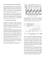
Fig. 1. Comparison between standard load profile and a real
load profile of a household
B. Simulation of low-voltage grids
The simulated low-voltage grid (Ur = 0.4 kV) in this
paper is based on a real existing grid in Germany. [2]
This grid is an urban grid which supplies a lot of
households in a small area. In this paper the load profile
generator is tested on a model of an urban low-voltage
grid including almost 80 connection points over an area
of 0.25 km². An average connection point supplies
approximately 10 households.
The program for the power flow simulation is done with
the tool MATPOWER. [3] This is a static calculation
program based on MATLAB. It simulates only one
moment of the power flow. To calculate the power flow
in the grid at various points in time with different loads,
an extension for MATPOWER was developed.
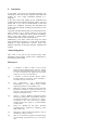
Figure 2 shows another extension developed by the
authors to interpret the simulated results. With this
extension it is possible to find critical situations, f.e. a
high utilization of the individual lines or the voltage drop
in the grid at each time step.
Fig. 2. Overview about the developed extension to interpret the
simulated results
3. Load Profile Generator
For this analysis a new behaviour based load profile
generator was used [4]. Most load profile generators
according to [1] are based on statistical approaches or
Markov chains.
One example is the program DHWCalc [5], a tool for
generating load profiles for domestic hot water use. It
works by assigning probabilities to time spans, for
example „50% between 12:00 and 13:00 on Weekdays“.
These probabilities are then used to randomly distribute
hot water usage events over all timespans, based on a
rather complicated algorithm. The algorithm takes into
account differences in winter and summer usage
behaviour, vacations and desired total yearly use.
Other load profile generators for electrical energy use
more complicated algorithms. Examples include finite
state machines or Markov chains, often coupled with
probabilities. A very simplified example of this might be
„After eating dinner there is an 80% chance of having the
TV turned on between 18:00 and 19:00, combined with a
30% of turning on the DVD player“. Those approaches
yield good results for creating a load profile for many
hundreds or thousands of households. But it is very
difficult to correctly simulate a realistic load profile for a
single household, especially for special cases like shift
workers or families with children.
Consider for example calculating the amortization time
of a battery used to raise the percentage of photovoltaic
power used in-house. It makes a large difference if the
household members are home during the day when the
sun is shining, if they work at nights or if they take 3
weeks of vacation in the summertime just when there is
the most sun.
The behaviour based load profile works differently: It
uses a psychological model based on the works of D.
Dörner [6] to simulate the behaviour of each member of
the household. From this the load profile
generator determines the device usage and then calculates
the energy profile.
Dörner’s work is based on the theory of the selfish homo
oeconomicus. The basic assumption here is that every
person always choses the action which best satisfies his
or her desires.
Dörner came up with a way to represent this very basic
idea with mathematical model in the computer: He
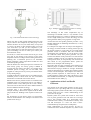
modelled each desire as “leaking water tank”. One of his
graphics is shown in Fig. 3. This means that the desire to
do something increases over time. It frequently needs to
be satisfied. And there is a logarithmic increase in the
importance of the desire the more urgent (empty) the
desire gets.