1
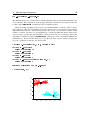
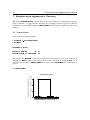
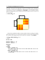
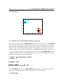
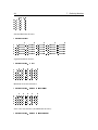
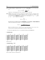
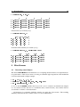
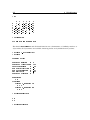
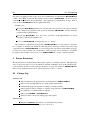
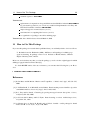
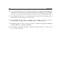
Software Manual
Institute of Bioinformatics, Johannes Kepler University Linz
APCluster
An R Package for Affinity Propagation Clustering
Ulrich Bodenhofer and Andreas Kothmeier
Institute of Bioinformatics, Johannes Kepler University Linz
Altenberger Str. 69, 4040 Linz, Austria
[email protected]
Version 1.1.0, June 10, 2011
Institute of Bioinformatics
Johannes Kepler University Linz
A-4040 Linz, Austria
Tel. +43 732 2468 8880
Fax +43 732 2468 9511
http://www.bioinf.jku.at
2
Contents
Scope and Purpose of this Document
This document is a user manual for the R package apcluster. It is only meant as a gentle introduction into how to use the basic functions implemented in this package. Not all features of
the R package are described in full detail. Such details can be obtained from the documentation
enclosed in the R package. Further note the following: (1) this is neither an introduction to affinity propagation nor to clustering in general; (2) this is not an introduction to R. If you lack the
background for understanding this manual, you first have to read introductory literature on these
subjects.
Contents
1
Introduction
3
2
Installation
2.1 Installation via CRAN . . . . . . . . . . . . . . . . . . . . . . . . . . . . . . .
2.2 Manual installation . . . . . . . . . . . . . . . . . . . . . . . . . . . . . . . . .
2.3 Compatibility issues . . . . . . . . . . . . . . . . . . . . . . . . . . . . . . . . .
3
3
3
4
3
Getting Started
4
4
Adjusting Input Preferences
9
5
Exemplar-based Agglomerative Clustering
5.1 Getting started . . . . . . . . . . . . . . . . . . . . . . . . . . . . . . . . . . . .
5.2 Merging clusters obtained from affinity propagation . . . . . . . . . . . . . . . .
5.3 Details on the merging objective . . . . . . . . . . . . . . . . . . . . . . . . . .
14
14
16
18
6
A Toy Example with Biological Sequences
19
7
Similarity Matrices
7.1 The function negDistMat() . . . . . . . . . . . . . . . . . . . . . . . . . . . .
7.2 Other similarity measures . . . . . . . . . . . . . . . . . . . . . . . . . . . . . .
24
24
27
8
Miscellaneous
8.1 Clustering named objects . . . . . . . . . . . . . . . . . . . . . . . . . . . . . .
8.2 Computing a label vector from a clustering result . . . . . . . . . . . . . . . . .
8.3 Performance issues . . . . . . . . . . . . . . . . . . . . . . . . . . . . . . . . .
29
29
31
31
9
Future Extensions
32
10 Change Log
32
11 How to Cite This Package
33
1
Introduction
1
Introduction
3
Affinity propagation (AP) is a relatively new clustering algorithm that has been introduced by
Brendan J. Frey and Delbert Dueck [3].1 The authors themselves describe affinity propagation as
follows:2
“An algorithm that identifies exemplars among data points and forms clusters of data
points around these exemplars. It operates by simultaneously considering all data
point as potential exemplars and exchanging messages between data points until a
good set of exemplars and clusters emerges.”
AP has been applied in various fields recently, among which bioinformatics is becoming increasingly important. Frey and Dueck have made their algorithm available as Matlab code.1 Matlab, however, is relatively uncommon in bioinformatics. Instead, the statistical computing platform
R has become a widely accepted standard in this field. In order to leverage affinity propagation
for bioinformatics applications, we have implemented affinity propagation as an R package. Note,
however, that the given package is in no way restricted to bioinformatics applications. It is as
generally applicable as Frey’s and Dueck’s original Matlab code.1
Starting with Version 1.1.0, the apcluster package also features exemplar-based agglomerative clustering which can be used as a clustering method on its own or for creating a hierarchy of
clusters that have been computed previously by affinity propagation.
2
Installation
2.1
Installation via CRAN
The R package apcluster (current version: 1.1.0) is part of the Comprehensive R Archive Network (CRAN)3 . The simplest way to install the package, therefore, is to enter the following command into your R session:
> install.packages("apcluster")
2.2
Manual installation
If, for what reason ever, you prefer to install the package manually, download the package file
suitable for your computer system and copy it to your harddisk. Open the package’s page at
CRAN4 and the proceed as follows.
http://www.psi.toronto.edu/affinitypropagation/
quoted from http://www.psi.toronto.edu/affinitypropagation/faq.html#def
3
http://cran.r-project.org/
4
http://cran.r-project.org/web/packages/apcluster/index.html
1
2
4
3
Getting Started
Manual installation under Windows
1. Download apcluster_1.1.0.zip and save it to your harddisk
2. Open the R GUI and select the menu entry
Packages | Install package(s) from local zip files...
(if you use R in a different language, search for the analogous menu entry). In the file dialog
that opens, go to the folder where you placed apcluster_1.1.0.zip and select this file.
The package should be installed now.
Manual installation under Linux/UNIX/MacOS
1. Download apcluster_1.1.0.tar.gz and save it to your harddisk.
2. Open a shell window and change to the directory where you put apcluster_1.1.0.tar.gz.
Enter
R CMD INSTALL apcluster_1.1.0.tar.gz
to install the package.
2.3
Compatibility issues
Both the Windows and the Linux/UNIX/MacOS version available from CRAN have been built
using the latest version, R 2.13.0. However, the package should work without severe problems on
R versions ≥2.10.1.
3
Getting Started
To load the package, enter the following in your R session:
> library(apcluster)
If this command terminates without any error message or warning, you can be sure that the package
has been installed successfully. If so, the package is ready for use now and you can start clustering
your data with affinity propagation.
The package includes both a user manual (this document) and a reference manual (help pages
for each function). To view the user manual, enter
> vignette("apcluster")
Help pages can be viewed using the help command. It is recommended to start with
> help(apcluster)
3
Getting Started
5
Affinity propagation does not require the data samples to be of any specific kind or structure.
AP only requires a similarity matrix, i.e., given l data samples, this is an l × l real-valued matrix
S, in which an entry Sij corresponds to a value measuring how similar sample i is to sample j.
AP does not require these values to be in a specific range. Values can be positive or negative. AP
does not even require the similarity matrix to be symmetric (although, in most applications, it will
be symmetric anyway). A value of −∞ is interpreted as “absolute dissimilarity”. The higher a
value, the more similar two samples are considered.
To get a first impression, let us create a random data set in R2 as the union of two “Gaussian
clouds”:
cl1 <- cbind(rnorm(30, 0.3, 0.05), rnorm(30, 0.7, 0.04))
cl2 <- cbind(rnorm(30, 0.7, 0.04), rnorm(30, 0.4, 0.05))
x1 <- rbind(cl1, cl2)
plot(x1, xlab = "", ylab = "", pch = 19, cex = 0.8)
0.8
>
>
>
>
●●
●●
●
●
●
●●
●● ●
● ●
●●
●
●
●●
●
●
●
●
●
●
●
0.5
0.6
0.7
●
●
●
●
●
●●
● ●
●
●●
0.4
●
●●
●●●●
0.3
●
●
● ●
●
●
0.3
0.4
0.5
0.6
0.7
●
●
●● ●
●
●
●
0.8
Now we have to create a similarity matrix. The package apcluster offers several different ways
for doing that (see Section 7 below). Let us start with the default similarity measure used in the
papers of Frey and Dueck — negative squared distances:
> s1 <- negDistMat(x1, r = 2)
We are now ready to run affinity propagation:
> apres1a <- apcluster(s1)
The function apcluster() creates an object belonging to the S4 class APResult which is defined
by the present package. To get detailed information on which data are stored in such objects, enter
6
3
Getting Started
> help(APResult)
The simplest thing we can do is to enter the name of the object (which implicitly calls show()) to
get a summary of the clustering result:
> apres1a
APResult object
Number of samples
Number of iterations
Input preference
Sum of similarities
Sum of preferences
Net similarity
Number of clusters
=
=
=
=
=
=
=
60
132
-0.1555249
-0.2556224
-0.3110499
-0.5666723
2
Exemplars:
28 32
Clusters:
Cluster 1, exemplar 28:
1 2 3 4 5 6 7 8 9 10 11 12 13 14 15 16 17 18 19 20 21 22 23 24 25 26
27 28 29 30
Cluster 2, exemplar 32:
31 32 33 34 35 36 37 38 39 40 41 42 43 44 45 46 47 48 49 50 51 52 53
54 55 56 57 58 59 60
For two-dimensional data sets, the apcluster package allows for plotting the original data set
along with a clustering result:
> plot(apres1a, x1)
Getting Started
7
0.8
3
●●
●●
●
●
●
●●
●● ●
● ●
●●
●
●
●●
●
●
●
●
●
●
●
0.5
0.6
0.7
●
●
●
●
●
●●
● ●
●
●●
0.4
●
●●
●●●●
0.3
●
●
● ●
●
●
0.3
0.4
0.5
0.6
●
●
●● ●
●
●
●
0.7
0.8
In this plot, each color corresponds to one cluster. The exemplar of each cluster is marked by a
box and all cluster members are connected to their exemplars with lines.
If plot() is called with the similarity matrix as second argument, a heatmap is created:
> plot(apres1a, s1)
1
2
3
4
5
6
7
8
9
10
11
12
13
14
15
16
17
18
19
20
21
22
23
24
25
26
27
28
29
30
31
32
33
34
35
36
37
38
39
40
41
42
43
44
45
46
47
48
49
50
51
52
53
54
55
56
57
58
59
60
1
2
3
4
5
6
7
8
9
10
11
12
13
14
15
16
17
18
19
20
21
22
23
24
25
26
27
28
29
30
31
32
33
34
35
36
37
38
39
40
41
42
43
44
45
46
47
48
49
50
51
52
53
54
55
56
57
58
59
60
In the heatmap, the samples are grouped according to clusters. The above heatmap confirms again
that there are two main clusters in the data.
Suppose we want to have better insight into what the algorithm did in each iteration. For this
purpose, we can supply the option details=TRUE to apcluster():
8
3
Getting Started
> apres1b <- apcluster(s1, details = TRUE)
This option tells the algorithm to keep a detailed log about its progress. For example, this allows
us to plot the three performance measures that AP uses internally for each iteration:
−4
−6
Fitness (overall net similarity)
Sum of exemplar preferences
Sum of similarities to exemplars
−8
Similarity
−2
0
> plot(apres1b)
0
20
40
60
80
100
120
# Iterations
These performance measures are:
1. Sum of exemplar preferences
2. Sum of similarities of exemplars to their cluster members
3. Net fitness: sum of the two former
For details, the user is referred to the original affinity propagation paper [3] and the supplementary
material published on the affinity propagation Web page.1 We see from the above plot that the
algorithm has not made any change for the last 100 (of 132!) iterations. AP, through its parameter
convits, allows to control for how long AP waits for a change until it terminates (the default is
convits=100). If the user has the feeling that AP will probably converge quicker on his/her data
set, a lower value can be used:
> apres1c <- apcluster(s1, convits = 15, details = TRUE)
> apres1c
APResult object
Number of samples
Number of iterations
Input preference
Sum of similarities
Sum of preferences
Net similarity
Number of clusters
=
=
=
=
=
=
=
60
47
-0.1555249
-0.2556224
-0.3110499
-0.5666723
2
4
Adjusting Input Preferences
9
Exemplars:
28 32
Clusters:
Cluster 1, exemplar 28:
1 2 3 4 5 6 7 8 9 10 11 12 13 14 15 16 17 18 19 20 21 22 23 24 25 26
27 28 29 30
Cluster 2, exemplar 32:
31 32 33 34 35 36 37 38 39 40 41 42 43 44 45 46 47 48 49 50 51 52 53
54 55 56 57 58 59 60
4
Adjusting Input Preferences
Apart from the similarity itself, the most important input parameter of AP is the so-called input
preference which can be interpreted as the tendency of a data sample to become an exemplar
(see [3] and supplementary material on the AP homepage1 for a more detailed explanation). This
input preference can either be chosen individually for each data sample or it can be a single value
shared among all data samples. Input preferences largely determine the number of clusters, in
other words, how fine- or coarse-grained the clustering result will be.
The input preferences one can specify for AP are roughly in the same range as the similarity
values, but they do not have a straightforward interpretation. Frey and Dueck have introduced the
following rule of thumb: “The shared value could be the median of the input similarities (resulting
in a moderate number of clusters) or their minimum (resulting in a small number of clusters).” [3]
Our AP implementation uses the median rule by default if the user does not supply a custom
value for the input preferences. In order to provide the user with a knob that is — at least to some
extent — interpretable, the function apcluster has a new argument q that allows to set the input
preference to a certain quantile of the input similarities: resulting in the median for q=0.5 and in
the minimum for q=0. As an example, let us add two more “clouds” to the data set from above:
>
>
>
>
>
cl3 <- cbind(rnorm(20, 0.5, 0.03), rnorm(20, 0.72, 0.03))
cl4 <- cbind(rnorm(25, 0.5, 0.03), rnorm(25, 0.42, 0.04))
x2 <- rbind(x1, cl3, cl4)
s2 <- negDistMat(x2, r = 2)
plot(x2, xlab = "", ylab = "", pch = 19, cex = 0.8)
4
0.8
10
●
●
●●
●●
●
●
●
●
●●
●● ●
● ●
●●
●
●
●●
●
●
●
●
●
●
● ●●
●
●● ● ●
●●● ● ●
●
●
●
●
●
0.5
0.6
0.7
●
●
●
Adjusting Input Preferences
●
●
●
●●
● ●
●
●●
●
●●
●●●●
●
●
● ●
●
●
0.3
0.4
●
●
●
●● ●
● ●
●●●
●
●
●
●
●
●
●
●●
●
●
●
●
0.3
0.4
0.5
0.6
●
●
●● ●
●
●
●
0.7
0.8
For the default setting, we obtain the following result:
0.8
> apres2a <- apcluster(s2)
> plot(apres2a, x2)
●●
●●
●
●
●
●
●●
●● ●
● ●
●●
●
●
●●
●
●
●
●
●
●
●
●
● ●●
●
●● ● ●
●●● ● ●
●
●
●
●
●
0.5
0.6
0.7
●
●
●
●
●
●●
● ●
●
●●
●
●●
●●●●
●
●
● ●
●
●
0.3
0.4
●
●
●
●
●
●
●● ●
● ●
●●●
●
●
●
●
●
●●
●●
●
●
0.3
0.4
0.5
0.6
●
●
●● ●
●
●
●
0.7
For the minimum of input similarities, we obtain the following result:
> apres2b <- apcluster(s2, q = 0)
> plot(apres2b, x2)
0.8
Adjusting Input Preferences
0.8
4
●
●
●
●
●
●●
●●
●
●
●
●
●●
●● ●
● ●
●●
●
●
●●
●
●
●
●
●
●
● ●●
●
●● ● ●
●●● ● ●
●
●
●
●
●
0.5
0.6
0.7
11
●
●
●
●●
● ●
●
●●
●
●●
●●●●
●
●
● ●
●
●
0.3
0.4
●
●
●
●● ●
● ●
●●●
●
●
●
●
●
●
●
●●
●
●
●
●
0.3
0.4
0.5
0.6
●
●
●● ●
●
●
●
0.7
0.8
So we see that AP is quite robust against a reduction of input preferences in this example which
may be caused by the clear separation of the four clusters. If we increase input preferences,
however, we can force AP to split the four clusters into smaller sub-clusters:
0.8
> apres2c <- apcluster(s2, q = 0.8)
> plot(apres2c, x2)
●●
●●
●
●
●
●
●●
●● ●
● ●
●●
●
●
●●
●
●
●
●
●
●
●
●
● ●●
●
●● ● ●
●●● ● ●
●
●
●
●
●
0.5
0.6
0.7
●
●
●
●
●
●●
● ●
●
●●
●
●●
●●●●
●
●
● ●
●
●
0.3
0.4
●
●
●
●
●
●
●● ●
● ●
●●●
●
●
●
●
●
●●
●●
●
●
0.3
0.4
0.5
0.6
0.7
●
●
●● ●
●
●
●
0.8
Note that the input preference used by AP can be recovered from the output object (no matter
which method to adjust input preferences has been used). On the one hand, the value is printed if
12
4
Adjusting Input Preferences
the object is displayed (by show or by entering the output object’s name). On the other hand, the
value can be accessed directly via the slot p:
> apres2c@p
[1] -0.01001869
As noted above already, we can produce a heatmap by calling plot() with an APResult
object as first and the corresponding similarity matrix as second argument:
> plot(apres2c, s2)
2
8
10
12
22
23
28
29
3
9
17
19
20
24
25
27
30
4
5
14
16
18
26
1
13
15
21
6
7
11
67
61
62
63
64
65
66
68
69
70
71
72
73
74
75
76
77
78
79
80
81
83
84
85
86
88
89
93
94
99
100
104
82
87
90
91
92
95
96
97
98
101
102
103
105
31
35
36
39
41
45
50
54
57
34
43
46
53
56
58
32
38
44
47
49
52
60
33
37
40
42
48
51
55
59
The order in which the clusters are arranged in the heatmap is determined by means of joining the
cluster agglomeratively (see Section 5 below). Although the affinity propagation result contains
12 clusters, the heatmap indicates that there are actually four clusters which can be seen as very
brightly colored squares along the diagonal. We also see that there seem to be two pairs of adjacent
clusters, which can be seen from the fact that there are two relatively light-colored blocks along
the diagonal encompassing two of the four clusters in each case. If we look back at how the data
have been created (see also plots above), this is exactly what is to be expected.
The above example with q=0 demonstrates that setting input preferences to the minimum of
input similarities does not necessarily result in a very small number of clusters (like one or two).
This is due to the fact that input preferences need not necessarily be exactly in the range of the
similarities. To determine a meaningful range, an auxiliary function is available which, in line
with Frey’s and Dueck’s Matlab code,1 allows to compute a minimum value (for which one or at
most two clusters would be obtained) and a maximum value (for which as many clusters as data
samples would be obtained):
> preferenceRange(s2)
4
Adjusting Input Preferences
13
[1] -5.727888e+00 -2.532793e-06
The function returns a two-element vector with the minimum value as first and the maximum value
as second entry. The computations are done approximately by default. If one is interested in exact
bounds, supply exact=TRUE (resulting in longer computation times).
Many clustering algorithms need to know a pre-defined number of clusters. This is often a
major nuisance, since the exact number of clusters is hard to know for non-trivial (in particular,
high-dimensional) data sets. AP avoids this problem. If, however, one still wants to require a fixed
number of clusters, this has to be accomplished by a search algorithm that adjusts input preferences in order to produce the desired number of clusters in the end. For convenience, this search
algorithm is available as a function apclusterK() (analogous to Frey’s and Dueck’s Matlab implementation1 ). We can use this function to force AP to produce only two clusters (merging the
two pairs of adjacent clouds into one cluster each):
> apres2d <- apclusterK(s2, K = 2, verbose = TRUE)
Trying p = -0.005730418
Number of clusters: 14
Trying p = -0.05728139
Number of clusters: 5
Trying p = -0.5727911
Number of clusters: 4
Trying p = -2.863945 (bisection step no. 1 )
Number of clusters: 2
Number of clusters: 2 for p = -2.863945
0.8
> plot(apres2d, x2)
●●
●●
●
●
●
●
●●
●● ●
● ●
●●
●
●
●●
●
●
●
●
●
●
●
●
● ●●
●
●● ● ●
●●● ● ●
●
●
●
●
●
0.5
0.6
0.7
●
●
●
●
●
0.3
0.4
0.5
●●
● ●
●
●●
●
●●
●●●●
●
●
● ●
●
●
0.3
0.4
●
●
●
●
●
●
●● ●
● ●
●●●
●
●
●
●
●
●●
●●
●
●
0.6
0.7
●
●
●● ●
●
●
●
0.8
14
5
5
Exemplar-based Agglomerative Clustering
Exemplar-based Agglomerative Clustering
The function aggExCluster() realizes what can best be described as “exemplar-based agglomerative clustering”, i.e. agglomerative clustering whose merging objective is geared towards the
identification of meaningful exemplars. aggExCluster() only requires a matrix of pairwise similarities.
5.1
Getting started
Let us start with a simple example:
> aggres1a <- aggExCluster(s1)
> aggres1a
AggExResult object
Number of samples
=
Maximum number of clusters =
60
60
The output object aggres1a contains the complete cluster hierarchy. As obvious from the above
example, the show() method only displays the most basic information. Calling plot() on an
object that was the result of aggExCluster() (an object of class AggExResult), a dendrogram is
plotted:
> plot(aggres1a)
−9.8e−02
−6.5e−02
50
57
45
35
54
31
39
36
41
40
46
53
34
58
43
56
49
38
47
52
32
44
60
33
51
55
42
59
37
48
7
6
11
10
12
23
28
29
2
22
27
30
19
3
9
20
25
17
24
26
5
16
18
4
14
13
21
1
8
15
−3.3e−02
−5.7e−06
Balanced avg. similarity to exemplar
Cluster dendrogram
5
Exemplar-based Agglomerative Clustering
15
The heights of the merges in the dendrogram correspond to the merging objective: the higher the
vertical bar of a merge, the less similar the two clusters have been. The dendrogram, therefore,
clearly indicates two clusters. Calling plot()for an AggExResult object along with the similarity
matrix as second argument produces a heatmap, where the dendrogram is plotted on top and to the
left of the heatmap:
> plot(aggres1a, s1)
50
57
45
35
54
31
39
36
41
40
46
53
34
58
43
56
49
38
47
52
32
44
60
33
51
55
42
59
37
48
7
6
11
10
12
23
28
29
2
22
27
30
19
3
9
20
25
17
24
26
5
16
18
4
14
13
21
1
8
15
50
57
45
35
54
31
39
36
41
40
46
53
34
58
43
56
49
38
47
52
32
44
60
33
51
55
42
59
37
48
7
6
11
10
12
23
28
29
2
22
27
30
19
3
9
20
25
17
24
26
5
16
18
4
14
13
21
1
8
15
Once we have confirmed the number of clusters, which is clearly 2 according to the dendrogram and the heatmap above, we can extract the level with two clusters from the cluster hierarchy.
In concordance with standard R terminology, the function for doing this is called cutree():
> cl1a <- cutree(aggres1a, k = 2)
> cl1a
ExClust object
Number of samples =
Number of clusters =
60
2
Exemplars:
32 28
Clusters:
Cluster 1, exemplar 32:
50 57 45 35 54 31 39 36 41 40 46 53 34 58 43 56 49 38 47 52 32 44 60
33 51 55 42 59 37 48
Cluster 2, exemplar 28:
7 6 11 10 12 23 28 29 2 22 27 30 19 3 9 20 25 17 24 26 5 16 18 4 14
13 21 1 8 15
16
5
Exemplar-based Agglomerative Clustering
0.8
> plot(cl1a, x1)
●
●
●●
●●
●
●●
●● ●
● ●
●●
●
●
●●
●
●
●
●
●
●
●
0.5
0.6
0.7
●
●
●
●
●
●●
● ●
●
●●
0.4
●
●●
●●●●
0.3
●
●
● ●
●
●
0.3
5.2
0.4
0.5
0.6
●
●
●● ●
●
●
0.7
●
0.8
Merging clusters obtained from affinity propagation
The most important application of aggExCluster() (and the reason why it is part of the apcluster
package) is that it can be used for creating a hierarchy of clusters starting from a set of clusters
previously computed by affinity propagation. The examples in Section 4 indicate that it may sometimes be tricky to define the right input preference. Exemplar-based agglomerative clustering on
affinity propagation results provides an additional tool for finding the right number of clusters.
Let us revisit the four-cluster example from Section 4. We can apply aggExCluster() to an
affinity propagation result if we run it on the same similarity matrix (as first argument) and supply
the affinity propagation result as second argument:
> aggres2a <- aggExCluster(s2, apres2c)
> aggres2a
AggExResult object
Number of samples
=
Maximum number of clusters =
105
12
The result apres2c had 12 clusters. aggExCluster() successively joins these clusters until only
one cluster is left. The dendrogram of this cluster hierarchy is given as follows:
> plot(aggres2a)
5
Exemplar-based Agglomerative Clustering
17
Cluster 8
Cluster 6
Cluster 9
Cluster 7
Cluster 12
Cluster 11
Cluster 1
Cluster 10
Cluster 4
Cluster 3
Cluster 5
Cluster 2
−0.0013
−0.0196
−0.0378
Balanced avg. similarity to exemplar
−0.0560
Cluster dendrogram
The following heatmap coincides with the one shown in Section 4 above. This is not surprising, since the heatmap plot for an affinity propagation result uses aggExCluster() internally to
arrange the clusters:
> plot(aggres2a, s2)
2
8
10
12
22
23
28
29
3
9
17
19
20
24
25
27
30
4
5
14
16
18
26
1
13
15
21
6
7
11
67
61
62
63
64
65
66
68
69
70
71
72
73
74
75
76
77
78
79
80
81
83
84
85
86
88
89
93
94
99
100
104
82
87
90
91
92
95
96
97
98
101
102
103
105
31
35
36
39
41
45
50
54
57
34
43
46
53
56
58
32
38
44
47
49
52
60
33
37
40
42
48
51
55
59
Once we are more or less sure about the number of clusters, we extract the right clustering
level from the hierarchy. For demonstation purposes, we do this for k = 5, . . . , 2 in the following
plots:
18
5
Exemplar-based Agglomerative Clustering
> par(mfrow = c(2, 2))
> for (k in 5:2) plot(aggres2a, x2, k = k, main = paste(k,
+
"clusters"))
●●
●●
0.8
●
●
●
●
●●
● ●●
●● ● ● ●
●
●●
●
●
●
●
●
●●
●
●● ● ●
●●● ● ●
● ●
●
●
●
●
●●
●●
●
●
●
●
●●
● ●●
●● ● ● ●
●
●●
●
●
●
●
●
●
●
0.5
0.5
●
●
●
●●
● ●
●
●●
●
●
● ●
●
●
0.4
0.5
0.6
●
●
●● ●
●
●
●
●
0.7
0.8
0.3
0.4
●
●
●
●
0.6
●
●
●
●
0.7
0.8
●
●●
●●
●
●
●
●
●●
● ●●
●● ● ● ●
●
●●
●
●
●
●
●
●
●
●
●
●
● ●●
●
●● ● ●
●●● ● ●
● ●
●
0.5
0.5
0.6
0.8
0.8
●
0.6
●●
● ●●
●● ● ● ●
●
●●
●
●
●
●
●●
●
●● ● ●
●●● ● ●
● ●
0.7
●
●
0.5
●
●● ●
●
●
●
●
●
●
●
●
●●
● ●
●
●●
●
●
● ●
●
●
0.3
0.4
0.5
0.6
0.7
●
●
●● ●
●
●
●
●●
● ●
●
●●
●
●
●
●
●
●● ●
● ●
●●
●
● ●
●
●
●
●
●
●●
●
●
●
●●
●●●●
●
●
● ●
●
●
●
●
●
0.3
●
●●
●●●●
0.3
0.4
●
●
●
●
●
●● ●
● ●
●●
●
● ●
●
●
●
●
●
●●
●
●
0.4
●●
●●
●
●
●
●
● ●
●
●
2 clusters
●
●
●●
● ●
●
●●
●
●●
●●●●
●
3 clusters
●
●
●
●
●
●
●
●● ●
● ●
●●
●
● ●
●
●
●
●
●
●●
●
●
0.3
●
●●
●●●●
0.3
0.4
●
●
●
●
●
●● ●
● ●
●●
●
● ●
●
●
●
●
●
●●
●
●
0.3
0.7
●
● ●●
●
●● ● ●
●●● ● ●
● ●
●
0.6
●
●
●
●
●
●
0.7
●
●
0.6
0.7
●
●
●
4 clusters
0.4
0.8
5 clusters
0.8
0.3
0.4
0.5
0.6
0.7
●
●
●● ●
●
●
●
0.8
There is one obvious, but important, condition: applying aggExCluster() to an affinity propagation result only makes sense if the number of clusters to start from is at least as large as the
number of true clusters in the data set. Clearly, if the number of clusters is already too small, then
merging will make the situation only worse.
5.3
Details on the merging objective
Like any other agglomerative clustering method (see, e.g., [4, 8, 10]), aggExCluster() merges
clusters until only one cluster containing all samples is obtained. In each step, two clusters
6
A Toy Example with Biological Sequences
19
are merged into one, i.e. the number of clusters is reduced by one. The only aspect in which
aggExCluster() differs from other methods is the merging objective.
Suppose we consider two clusters for possible merging, each of which is given by an index
set:
I = {i1 , . . . , inI } and J = {j1 , . . . , jnJ }
Then we first determine the potential joint exemplar ex(I, J) as the sample that maximizes the
average similarity to all samples in the joint cluster I ∪ J:
ex(I, J) = argmax
i∈I∪J
X
1
·
Sij
nI + nJ
j∈I∪J
Recall that S denotes the similarity matrix and Sij corresponds to the similarity of the i-th and the
j-th sample. Then the merging objective is computed as
obj(I, J) =
1 1 X
1 X
·
Sex(I,J)j +
·
Sex(I,J)k ,
·
2
nI
nJ
j∈I
k∈J
which can be best described as “balanced average similarity to the joint exemplar”. In each step,
aggExCluster() considers all pairs of clusters in the current cluster set and joins that pair of
clusters whose merging objective is maximal. The rationale behind the merging objective is that
those two clusters should be joined that are best described by a joint exemplar.
6
A Toy Example with Biological Sequences
As noted in the introduction above, one of the goals of this package is to leverage affinity propagation in bioinformatics applications. In order to demonstrate the usage of the package in a biological
application, we consider a small toy example here.
The package comes with a toy data set ch22Promoters that consists of promoter regions of
150 random genes from the human chromosome no. 22 (according to the human genome assembly
hg18). Each sequence consists of the 1000 bases upstream of the transcription start site of each
gene. Suppose we want to cluster these sequences in order to find out whether groups of promoters
can be identified on the basis of the sequence only and, if so, to identify exemplars that are most
typical for these groups.
> data(ch22Promoters)
> names(ch22Promoters)[1:5]
[1] "NM_001169111" "NM_012324"
[5] "NM_001184970"
"NM_144704"
"NM_002473"
> substr(ch22Promoters[1:5], 951, 1000)
NM_001169111
"GCACGCGCTGAGAGCCTGTCAGCGGCTGCGCCCGTGTGCGCATGCGCAGC"
20
6
A Toy Example with Biological Sequences
NM_012324
"CCGCCTCCCCCGCCGCCCTCCCCGCGCCGCCGCGGAGTCCGGGCGAGGTG"
NM_144704
"GTGCTGGGCCCGCGGGCTCCCCGGCCGCAGTGCAAACGCAGCGCCAGACA"
NM_002473
"CAGGCTCCGCCCCGGAGCCGGCTCCCGGCTGGGAATGGTCCCGCGGCTCC"
NM_001184970
"GGGGCGGGGCTCGGTGTCCGGTAGCCAATGGACAGAGCCCAGCGGGAGCG"
Obviously, these are classical nucleotide sequences, each of which is identified by the RefSeq
identifier of the gene the promoter sequence stems from.
In order to compute a similarity matrix for this data set, we choose (without further justification, just for demonstration purposes) the simple spectrum kernel [6] with a sub-sequence length
of k = 6. We use the implementation from the kernlab package [5] to compute the similarity
matrix in a convenient way:
>
>
+
>
>
library(kernlab)
promSim <- kernelMatrix(stringdot(length = 6, type = "spectrum"),
ch22Promoters)
rownames(promSim) <- names(ch22Promoters)
colnames(promSim) <- names(ch22Promoters)
Now we run affinity propagation on this similarity matrix:
> promAP <- apcluster(promSim, q = 0)
> promAP
APResult object
Number of samples
Number of iterations
Input preference
Sum of similarities
Sum of preferences
Net similarity
Number of clusters
=
=
=
=
=
=
=
150
185
0.01367387
57.76715
0.109391
57.87655
8
Exemplars:
NM_001199580 NM_022141 NM_152868 NM_001128633 NM_052945 NM_001099294
NM_152513 NM_080764
Clusters:
Cluster 1, exemplar NM_001199580:
NM_001169111 NM_012324 NM_144704 NM_002473 NM_005198 NM_004737
NM_007194 NM_014292 NM_001199580 NM_032758 NM_003325 NM_014876
NM_000407 NM_053004 NM_023004 NM_001130517 NM_002882 NM_001169110
NM_020831 NM_001195071 NM_031937 NM_001164502 NM_152299 NM_014509
6
A Toy Example with Biological Sequences
21
NM_138433 NM_006487 NM_005984 NM_001085427 NM_013236
Cluster 2, exemplar NM_022141:
NM_001184970 NM_002883 NM_001051 NM_014460 NM_153615 NM_022141
NM_001137606 NM_001184971 NM_053006 NM_015367 NM_000395 NM_012143
NM_004147
Cluster 3, exemplar NM_152868:
NM_015140 NM_138415 NM_001195072 NM_001164501 NM_014339 NM_152868
NM_033257 NM_014941 NM_033386 NM_007311 NM_017911 NM_007098
NM_001670 NM_015653 NM_032775 NM_001172688 NM_001136029 NM_001024939
NM_002969 NM_052906 NM_152511 NM_001001479
Cluster 4, exemplar NM_001128633:
NM_001128633 NM_002133 NM_015672 NM_013378 NM_001128633 NM_000106
NM_152855
Cluster 5, exemplar NM_052945:
NM_001102371 NM_017829 NM_020243 NM_002305 NM_030882 NM_000496
NM_022720 NM_024053 NM_052945 NM_018006 NM_014433 NM_032561
NM_001142964 NM_181492 NM_003073 NM_015366 NM_005877 NM_148674
NM_005008 NM_017414 NM_000185 NM_001135911 NM_001199562 NM_003935
NM_003560 NM_001166242 NM_001165877
Cluster 6, exemplar NM_001099294:
NM_004900 NM_001097 NM_174975 NM_004377 NM_001099294 NM_004121
NM_001146288 NM_002415 NM_001159546 NM_004327 NM_152426 NM_004861
NM_001193414 NM_001145398 NM_015715 NM_021974 NM_001159554
NM_001171660 NM_015124 NM_006932 NM_152906 NM_001002034 NM_000754
NM_145343
Cluster 7, exemplar NM_152513:
NM_001135772 NM_007128 NM_014227 NM_203377 NM_152267 NM_017590
NM_001098270 NM_138481 NM_012401 NM_014303 NM_001144931 NM_001098535
NM_000262 NM_152510 NM_003347 NM_001039141 NM_001014440 NM_152513
NM_015330 NM_138338 NM_032608
Cluster 8, exemplar NM_080764:
NM_175878 NM_003490 NM_001039366 NM_001010859 NM_014306 NM_080764
NM_001164104
So we obtain 8 clusters in total. The corresponding heatmap looks as follows:
> plot(promAP, promSim)
22
6
A Toy Example with Biological Sequences
NM_175878
NM_003490
NM_001039366
NM_001010859
NM_014306
NM_080764
NM_001164104
NM_001135772
NM_007128
NM_014227
NM_203377
NM_152267
NM_017590
NM_001098270
NM_138481
NM_012401
NM_014303
NM_001144931
NM_001098535
NM_000262
NM_152510
NM_003347
NM_001039141
NM_001014440
NM_152513
NM_015330
NM_138338
NM_032608
NM_001184970
NM_002883
NM_001051
NM_014460
NM_153615
NM_022141
NM_001137606
NM_001184971
NM_053006
NM_015367
NM_000395
NM_012143
NM_004147
NM_001128633
NM_002133
NM_015672
NM_013378
NM_001128633
NM_000106
NM_152855
NM_001169111
NM_012324
NM_144704
NM_002473
NM_005198
NM_004737
NM_007194
NM_014292
NM_001199580
NM_032758
NM_003325
NM_014876
NM_000407
NM_053004
NM_023004
NM_001130517
NM_002882
NM_001169110
NM_020831
NM_001195071
NM_031937
NM_001164502
NM_152299
NM_014509
NM_138433
NM_006487
NM_005984
NM_001085427
NM_013236
NM_015140
NM_138415
NM_001195072
NM_001164501
NM_014339
NM_152868
NM_033257
NM_014941
NM_033386
NM_007311
NM_017911
NM_007098
NM_001670
NM_015653
NM_032775
NM_001172688
NM_001136029
NM_001024939
NM_002969
NM_052906
NM_152511
NM_001001479
NM_001102371
NM_017829
NM_020243
NM_002305
NM_030882
NM_000496
NM_022720
NM_024053
NM_052945
NM_018006
NM_014433
NM_032561
NM_001142964
NM_181492
NM_003073
NM_015366
NM_005877
NM_148674
NM_005008
NM_017414
NM_000185
NM_001135911
NM_001199562
NM_003935
NM_003560
NM_001166242
NM_001165877
NM_004900
NM_001097
NM_174975
NM_004377
NM_001099294
NM_004121
NM_001146288
NM_002415
NM_001159546
NM_004327
NM_152426
NM_004861
NM_001193414
NM_001145398
NM_015715
NM_021974
NM_001159554
NM_001171660
NM_015124
NM_006932
NM_152906
NM_001002034
NM_000754
NM_145343
Let us now run agglomerative clustering to further join clusters.
> promAgg <- aggExCluster(promSim, promAP)
The resulting dendrogram is given as follows:
> plot(promAgg)
0.25
0.30
0.36
Cluster 6
Cluster 5
Cluster 3
Cluster 1
Cluster 4
Cluster 2
Cluster 7
Cluster 8
0.42
Balanced avg. similarity to exemplar
Cluster dendrogram
The dendrogram does not give a very clear indication about the best number of clusters. Let us
adopt the viewpoint for a moment that 5 clusters are reasonable.
6
A Toy Example with Biological Sequences
23
> prom5 <- cutree(promAgg, k = 5)
> prom5
ExClust object
Number of samples =
Number of clusters =
150
5
Exemplars:
NM_152513 NM_080764 NM_001128633 NM_001199580 NM_052945
Clusters:
Cluster 1, exemplar NM_152513:
NM_001135772 NM_007128 NM_014227 NM_203377 NM_152267 NM_017590
NM_001098270 NM_138481 NM_012401 NM_014303 NM_001144931 NM_001098535
NM_000262 NM_152510 NM_003347 NM_001039141 NM_001014440 NM_152513
NM_015330 NM_138338 NM_032608
Cluster 2, exemplar NM_080764:
NM_175878 NM_003490 NM_001039366 NM_001010859 NM_014306 NM_080764
NM_001164104
Cluster 3, exemplar NM_001128633:
NM_001184970 NM_002883 NM_001051 NM_014460 NM_153615 NM_022141
NM_001137606 NM_001184971 NM_053006 NM_015367 NM_000395 NM_012143
NM_004147 NM_001128633 NM_002133 NM_015672 NM_013378 NM_001128633
NM_000106 NM_152855
Cluster 4, exemplar NM_001199580:
NM_001169111 NM_012324 NM_144704 NM_002473 NM_005198 NM_004737
NM_007194 NM_014292 NM_001199580 NM_032758 NM_003325 NM_014876
NM_000407 NM_053004 NM_023004 NM_001130517 NM_002882 NM_001169110
NM_020831 NM_001195071 NM_031937 NM_001164502 NM_152299 NM_014509
NM_138433 NM_006487 NM_005984 NM_001085427 NM_013236 NM_015140
NM_138415 NM_001195072 NM_001164501 NM_014339 NM_152868 NM_033257
NM_014941 NM_033386 NM_007311 NM_017911 NM_007098 NM_001670
NM_015653 NM_032775 NM_001172688 NM_001136029 NM_001024939 NM_002969
NM_052906 NM_152511 NM_001001479
Cluster 5, exemplar NM_052945:
NM_001102371 NM_017829 NM_020243 NM_002305 NM_030882 NM_000496
NM_022720 NM_024053 NM_052945 NM_018006 NM_014433 NM_032561
NM_001142964 NM_181492 NM_003073 NM_015366 NM_005877 NM_148674
NM_005008 NM_017414 NM_000185 NM_001135911 NM_001199562 NM_003935
NM_003560 NM_001166242 NM_001165877 NM_004900 NM_001097 NM_174975
NM_004377 NM_001099294 NM_004121 NM_001146288 NM_002415 NM_001159546
NM_004327 NM_152426 NM_004861 NM_001193414 NM_001145398 NM_015715
NM_021974 NM_001159554 NM_001171660 NM_015124 NM_006932 NM_152906
NM_001002034 NM_000754 NM_145343
The final heatmap looks as follows:
24
7
Similarity Matrices
> plot(prom5, promSim)
NM_175878
NM_003490
NM_001039366
NM_001010859
NM_014306
NM_080764
NM_001164104
NM_001135772
NM_007128
NM_014227
NM_203377
NM_152267
NM_017590
NM_001098270
NM_138481
NM_012401
NM_014303
NM_001144931
NM_001098535
NM_000262
NM_152510
NM_003347
NM_001039141
NM_001014440
NM_152513
NM_015330
NM_138338
NM_032608
NM_001184970
NM_002883
NM_001051
NM_014460
NM_153615
NM_022141
NM_001137606
NM_001184971
NM_053006
NM_015367
NM_000395
NM_012143
NM_004147
NM_001128633
NM_002133
NM_015672
NM_013378
NM_001128633
NM_000106
NM_152855
NM_001169111
NM_012324
NM_144704
NM_002473
NM_005198
NM_004737
NM_007194
NM_014292
NM_001199580
NM_032758
NM_003325
NM_014876
NM_000407
NM_053004
NM_023004
NM_001130517
NM_002882
NM_001169110
NM_020831
NM_001195071
NM_031937
NM_001164502
NM_152299
NM_014509
NM_138433
NM_006487
NM_005984
NM_001085427
NM_013236
NM_015140
NM_138415
NM_001195072
NM_001164501
NM_014339
NM_152868
NM_033257
NM_014941
NM_033386
NM_007311
NM_017911
NM_007098
NM_001670
NM_015653
NM_032775
NM_001172688
NM_001136029
NM_001024939
NM_002969
NM_052906
NM_152511
NM_001001479
NM_001102371
NM_017829
NM_020243
NM_002305
NM_030882
NM_000496
NM_022720
NM_024053
NM_052945
NM_018006
NM_014433
NM_032561
NM_001142964
NM_181492
NM_003073
NM_015366
NM_005877
NM_148674
NM_005008
NM_017414
NM_000185
NM_001135911
NM_001199562
NM_003935
NM_003560
NM_001166242
NM_001165877
NM_004900
NM_001097
NM_174975
NM_004377
NM_001099294
NM_004121
NM_001146288
NM_002415
NM_001159546
NM_004327
NM_152426
NM_004861
NM_001193414
NM_001145398
NM_015715
NM_021974
NM_001159554
NM_001171660
NM_015124
NM_006932
NM_152906
NM_001002034
NM_000754
NM_145343
7
Similarity Matrices
Apart from the obvious monotonicity “the higher the value, the more similar two samples”, affinity propagation does not make any specific assumption about the similarity measure. Negative
squared distances must be used if one wants to minimize squared errors [3]. Apart from that, the
choice and implementation of the similarity measure is left to the user.
Our package offers a few more methods to obtain similarity matrices. The choice of the right
one (and, consequently, the objective function the algorithm optimizes) still has to be made by the
user.
All functions described in this section assume the input data matrix to be organized such that
each row corresponds to one sample and each column corresponds to one feature (in line with the
standard function dist). If a vector is supplied instead of a matrix, each single entry is interpreted
as a (one-dimensional) sample.
7.1
The function negDistMat()
The function negDistMat(), in line with Frey and Dueck, allows for computing negative distances for a given set of real-valued data samples. Above we have used the following:
> s2 <- negDistMat(x2, r = 2)
This computes a matrix of negative squared distances from the data matrix x. The function
negDistMat() is a simple wrapper around the standard function dist(), hence, it allows for
7
Similarity Matrices
25
a lot more different similarity measures. The user can make use of all variants implemented
in dist() by using the options method (selects a distance measure) and p (specifies the exponent for the Minkowski distance, otherwise it is void) that are passed on to dist(). Presently,
dist() provides the following variants of computing the distance d(x, y) of two data samples
x = (x1 , . . . , xn ) and y = (y1 , . . . , yn ):
Euclidean:
v
u n
uX
d(x, y) = t (xi − yi )2
i=1
use method="euclidean" or do not specify argument method (since this is the default);
Maximum:
n
d(x, y) = max |xi − yi |
i=1
use method="maximum";
Sum of absolute distances / Manhattan:
d(x, y) =
n
X
|xi − yi |
i=1
use method="manhattan";
Canberra:
d(x, y) =
n
X
|xi − yi |
i=1
|xi + yi |
summands with zero denominators are not taken into account; use method="canberra";
Minkowski:
d(x, y) =
n
X
(xi − yi )p
!1
p
i=1
use method="minkowski" and specify p using the additional argument p (default is p=2,
resulting in the standard Euclidean distance);
We do not consider method="binary" here, since it is irrelevant for real-valued data.
The function negDistMat() takes the distances computed with one of the variants listed above
and returns −1 times the r-th power of it, i.e.,
s(x, y) = −d(x, y)r .
(1)
The exponent r can be adjusted with the argument r. The default is r=1, hence, one has to supply
r=2 as in the above example to obtain squared distances.
Here are some examples. We use the corners of the two-dimensional unit square and its middle
point ( 21 , 12 ) as sample data:
> ex <- matrix(c(0, 0, 1, 0, 0.5, 0.5, 0, 1, 1, 1), 5, 2, byrow = TRUE)
> ex
26
[1,]
[2,]
[3,]
[4,]
[5,]
7
[,1]
0.0
1.0
0.5
0.0
1.0
[,2]
0.0
0.0
0.5
1.0
1.0
Standard Euclidean distance:
> negDistMat(ex)
1
2
3
4
5
1
0.0000000
-1.0000000
-0.7071068
-1.0000000
-1.4142136
2
-1.0000000
0.0000000
-0.7071068
-1.4142136
-1.0000000
3
-0.7071068
-0.7071068
0.0000000
-0.7071068
-0.7071068
4
-1.0000000
-1.4142136
-0.7071068
0.0000000
-1.0000000
Squared Euclidean distance:
> negDistMat(ex, r = 2)
1
2
3
4
5
1
0.0
-1.0
-0.5
-1.0
-2.0
2
-1.0
0.0
-0.5
-2.0
-1.0
3
-0.5
-0.5
0.0
-0.5
-0.5
4
-1.0
-2.0
-0.5
0.0
-1.0
5
-2.0
-1.0
-0.5
-1.0
0.0
Maximum norm-based distance:
> negDistMat(ex, method = "maximum")
1
2
3
4
5
1
0.0
-1.0
-0.5
-1.0
-1.0
2
-1.0
0.0
-0.5
-1.0
-1.0
3
-0.5
-0.5
0.0
-0.5
-0.5
4
-1.0
-1.0
-0.5
0.0
-1.0
5
-1.0
-1.0
-0.5
-1.0
0.0
Sum of absolute distances (aka Manhattan distance):
> negDistMat(ex, method = "manhattan")
5
-1.4142136
-1.0000000
-0.7071068
-1.0000000
0.0000000
Similarity Matrices
7
1
2
3
4
5
Similarity Matrices
1
0
-1
-1
-1
-2
2
-1
0
-1
-2
-1
3
-1
-1
0
-1
-1
4
-1
-2
-1
0
-1
27
5
-2
-1
-1
-1
0
Canberra distance:
> negDistMat(ex, method = "canberra")
1
2
3
4
5
1
0
-2
-2
-2
-2
2
-2.000000
0.000000
-1.333333
-2.000000
-1.000000
3
-2.0000000
-1.3333333
0.0000000
-1.3333333
-0.6666667
4
-2.000000
-2.000000
-1.333333
0.000000
-1.000000
5
-2.0000000
-1.0000000
-0.6666667
-1.0000000
0.0000000
Minkowski distance for p = 3 (3-norm):
> negDistMat(ex, method = "minkowski", p = 3)
1
2
3
4
5
1
0.0000000
-1.0000000
-0.6299605
-1.0000000
-1.2599210
7.2
2
-1.0000000
0.0000000
-0.6299605
-1.2599210
-1.0000000
3
-0.6299605
-0.6299605
0.0000000
-0.6299605
-0.6299605
4
-1.0000000
-1.2599210
-0.6299605
0.0000000
-1.0000000
5
-1.2599210
-1.0000000
-0.6299605
-1.0000000
0.0000000
Other similarity measures
The package apcluster offers three more functions for creating similarity matrices for realvalued data:
Exponential transformation of distances: the function expSimMat() is another wrapper around
the standard function dist(). The difference is that, instead of the transformation (1), it
uses the following transformation:
d(x, y) r
s(x, y) = exp −
w
Here the default is r=2. It is clear that r=2 in conjunction with method="euclidean"
results in the well-known Gaussian kernel / RBF kernel [2, 7, 9], whereas r=1 in conjunction with method="euclidean" results in the similarity measure that is sometimes called
Laplace kernel [2, 7]. Both variants (for non-Euclidean distances as well) can also be interpreted as fuzzy equality/similarity relations [1].
28
7
Similarity Matrices
Linear scaling of distances with truncation: the function linSimMat() uses the transformation
d(x, y)
s(x, y) = max 1 −
,0
w
which is also often interpreted as a fuzzy equality/similarity relation [1].
Linear kernel: scalar products can also be interpreted as similarity measures, a view that is often
adopted by kernel methods in machine learning. In order to provide the user with this option
as well, the function linKernel() is available. For two data samples x = (x1 , . . . , xn ) and
y = (y1 , . . . , yn ), it computes the similarity as
s(x, y) =
n
X
xi · yi .
i=1
The function has one additional argument, normalize (by default FALSE). If normalize=TRUE,
values are normalized to the range [−1, +1] in the following way:
Pn
xi · yi
s(x, y) = q P i=1 P
n
n
2
2
i=1 yi
i=1 xi ·
Entries for which at least one of the two factors in the denominator is zero are set to zero
(however, the user should be aware that this should be avoided anyway).
For the same example data as above, we obtain the following for the RBF kernel:
> expSimMat(ex)
1
2
3
4
5
1
1.0000000
0.3678794
0.6065307
0.3678794
0.1353353
2
0.3678794
1.0000000
0.6065307
0.1353353
0.3678794
3
0.6065307
0.6065307
1.0000000
0.6065307
0.6065307
4
0.3678794
0.1353353
0.6065307
1.0000000
0.3678794
5
0.1353353
0.3678794
0.6065307
0.3678794
1.0000000
3
0.4930687
0.4930687
1.0000000
0.4930687
0.4930687
4
0.3678794
0.2431167
0.4930687
1.0000000
0.3678794
5
0.2431167
0.3678794
0.4930687
0.3678794
1.0000000
Laplace kernel:
> expSimMat(ex, r = 1)
1
2
3
4
5
1
1.0000000
0.3678794
0.4930687
0.3678794
0.2431167
2
0.3678794
1.0000000
0.4930687
0.2431167
0.3678794
Linear scaling of distances with truncation:
8
Miscellaneous
29
> linSimMat(ex, w = 1.2)
1
2
3
4
5
1
1.0000000
0.1666667
0.4107443
0.1666667
0.0000000
2
0.1666667
1.0000000
0.4107443
0.0000000
0.1666667
3
0.4107443
0.4107443
1.0000000
0.4107443
0.4107443
4
0.1666667
0.0000000
0.4107443
1.0000000
0.1666667
5
0.0000000
0.1666667
0.4107443
0.1666667
1.0000000
Linear kernel (we exclude (0, 0)):
> linKernel(ex[2:5, ])
[1,]
[2,]
[3,]
[4,]
[,1]
1.0
0.5
0.0
1.0
[,2]
0.5
0.5
0.5
1.0
[,3] [,4]
0.0
1
0.5
1
1.0
1
1.0
2
Normalized linear kernel (we exclude (0, 0)):
> linKernel(ex[2:5, ], normalize = TRUE)
[1,]
[2,]
[3,]
[4,]
8
8.1
[,1]
1.0000000
0.7071068
0.0000000
0.7071068
[,2]
0.7071068
1.0000000
0.7071068
1.0000000
[,3]
0.0000000
0.7071068
1.0000000
0.7071068
[,4]
0.7071068
1.0000000
0.7071068
1.0000000
Miscellaneous
Clustering named objects
The function apcluster() and all functions for computing distance matrices are implemented to
recognize names of data objects and to correctly pass them through computations. The mechanism
is best described with a simple example:
> x3 <- c(1, 2, 3, 7, 8, 9)
> names(x3) <- c("a", "b", "c", "d", "e", "f")
> s3 <- negDistMat(x3, r = 2)
So we see that the names attribute must be used if a vector of named one-dimensional samples
is to be clustered. If the data are not one-dimensional (a matrix instead), object names must be
stored in the row names of the data matrix.
All functions for computing similarity matrices recognize the object names. The resulting
similarity matrix has the list of names both as row and column names.
30
8
Miscellaneous
> s3
a
b
c
d
e
f
a
0
-1
-4
-36
-49
-64
b
-1
0
-1
-25
-36
-49
c
-4
-1
0
-16
-25
-36
d
-36
-25
-16
0
-1
-4
e
-49
-36
-25
-1
0
-1
f
-64
-49
-36
-4
-1
0
> colnames(s3)
[1] "a" "b" "c" "d" "e" "f"
The function apcluster() and all related functions use column names of similarity matrices as
object names. If object names are available, clustering results are by default shown by names.
> apres3a <- apcluster(s3)
> apres3a
APResult object
Number of samples
Number of iterations
Input preference
Sum of similarities
Sum of preferences
Net similarity
Number of clusters
=
=
=
=
=
=
=
6
124
-25
-4
-50
-54
2
Exemplars:
b e
Clusters:
Cluster 1, exemplar b:
a b c
Cluster 2, exemplar e:
d e f
> apres3a@exemplars
b e
2 5
> apres3a@clusters
8
Miscellaneous
31
[[1]]
a b c
1 2 3
[[2]]
d e f
4 5 6
8.2
Computing a label vector from a clustering result
For later classification or comparisons with other clustering methods, it may be useful to compute
a label vector from a clustering result. Our package provides an instance of the generic function
labels() for this task. As obvious from the following example, the argument type can be used
to determine how to compute the label vector.
> apres3a@exemplars
b e
2 5
> labels(apres3a, type = "names")
[1] "b" "b" "b" "e" "e" "e"
> labels(apres3a, type = "exemplars")
[1] 2 2 2 5 5 5
> labels(apres3a, type = "enum")
[1] 1 1 1 2 2 2
The first choice, "names" (default), uses names of exemplars as labels (if names are available,
otherwise an error message is displayed). The second choice, "exemplars", uses indices of exemplars (enumerated as in the original data set). The third choice, "enum", uses indices of clusters
(consecutively numbered as stored in the slot clusters; analogous to the standard implementation of cutree() or the clusters field of the list returned by the standard function kmeans()).
8.3
Performance issues
Starting with version 1.0.2, the function apcluster() uses pure matrix operations for computing
responsibilities and availabilities in the affinity propagation main loop. While this normally leads
to significant performance improvements, it also results in an increased consumption of memory
for storing intermediate results. For large data sets of several thousands of samples and more, this
32
10 Change Log
may lead to swapping.5 If this occurs, users are recommended to use the function apclusterLM()
(“LM” = Less Memory) instead. This function works exactly as apcluster(), but uses loops for
computing responsibilities and availabilities, only requiring O(l) intermediate storage. In most
cases, however, apcluster() will be significantly faster.
Further notes:
The function apcluster() makes use of matrix and vector operations. If your R system has
been configured to parallelize such operations internally, apcluster() will automatically
benefit from this parallelization.
Even though apcluster() uses only vector operations, our R implementation is slower
than Frey’s and Dueck’s Matlab code.1
Do not use details=TRUE for larger data sets (l > 1000)!
The asymptotic computational complexity of aggExCluster() is O(l3 ) (where l is the number of samples or clusters from which the clustering starts). This may result in excessively long
computation times if aggExCluster() is used for larger data sets without using affinity propagation first. For real-world data sets, in particular, if they are large, we recommend to use affinity
propagation first and then, if necessary, to use aggExCluster() to create a cluster hierarchy.
9
Future Extensions
We currently have no implementation that exploits sparsity of similarity matrices. The implementation of sparse AP and leveraged AP which are available as Matlab code from the AP Web page1
is left for future extensions of the package. Presently, we only offer a function sparseToFull()
that converts similarity matrices from sparse format into a full l × l matrix.
10
Change Log
Version 1.1.0:
added exemplar-based agglomerative clustering function aggExCluster()
added various plotting functions for dendrograms and heatmaps
extended help pages and vignette according to new functionality
added sequence analysis example to vignette along with data set ch22Promoters
re-organization of variable names in vignette
added option verbose to apclusterK()
numerous minor corrections in help pages and vignette
Version 1.0.3:
Makefile in inst/doc eliminated to avoid installation problems
5
depending on available main memory, operating system, and R version
11
How to Cite This Package
33
renamed vignette to “apcluster”
Version 1.0.2:
replacement of computation of responsibilities and availabilities in function apcluster()
by pure matrix operations (see 8.3 above); traditional implementation à la Frey and
Dueck still available as function apclusterLM;
improved support for named objects (see 8.1)
new function for computing label vectors (see 8.2)
re-organization of package source files and help pages
Version 1.0.1: first official release, released March 2, 2010
11
How to Cite This Package
If you use this package for research that is published later, you are kindly asked to cite it as follows:
U. Bodenhofer and A. Kothmeier (2010). APCluster: an R package for affinity propagation clustering. R package version 1.1.0. Institute of Bioinformatics, Johannes
Kepler University, Linz, Austria.
Moreover, we insist that, any time you cite the package, you also cite the original paper in which
affinity propagation has been introduced [3].
To obtain BibTEX entries of the two references, you can enter the following into your R session:
> toBibtex(citation("apcluster"))
References
[1] B. De Baets and R. Mesiar. Metrics and T -equalities. J. Math. Anal. Appl., 267:531–547,
2002.
[2] C. H. FitzGerald, C. A. Micchelli, and A. Pinkus. Functions that preserve families of positive
semidefinite matrices. Linear Alg. Appl., 221:83–102, 1995.
[3] B. J. Frey and D. Dueck. Clustering by passing messages between data points. Science,
315(5814):972–976, 2007.
[4] A. K. Jain, M. N. Murty, and P. J. Flynn. Data clustering: a review. ACM Comput. Surv.,
31(3):264–323, 1999.
[5] A. Karatzoglou, A. Smola, K. Hornik, and A. Zeileis. kernlab – an S4 package for kernel
methods in R. J. Stat. Softw., 11(9):1–20, 2004.
34
References
[6] C. Leslie, E. Eskin, and W. S. Noble. The spectrum kernel: a string kernel for SVM protein
classification. In R. B. Altman, A. K. Dunker, L. Hunter, K. Lauderdale, and T. E. D. Klein,
editors, Pacific Symposium on Biocomputing 2002, pages 566–575. World Scientific, 2002.
[7] C. A. Micchelli. Interpolation of scattered data: Distance matrices and conditionally positive
definite functions. Constr. Approx., 2:11–22, 1986.
[8] R. S. Michalski and R. E. Stepp. Clustering. In S. C. Shapiro, editor, Encyclopedia of
artificial intelligence, pages 168–176. John Wiley & Sons, Chichester, 1992.
[9] B. Schölkopf and A. J. Smola. Learning with Kernels. Adaptive Computation and Machine
Learning. MIT Press, Cambridge, MA, 2002.
[10] J. H. Ward Jr. Hierarchical grouping to optimize an objective function. J. Amer. Statist.
Assoc., 58:236–244, 1963.