Download AHAS (AVHRR Hydrological Analysis System)

AHVRR Hydrological Analysis System
User Manual Version 1.3
WRES – ITC 2002
by Ir. Gabriel Parodi
AHAS User Guide
AHAS User Guide
Credits and acknowledgments
This software compiles more than 60 different methodologies developed by hundreds of authors.
Without their intensive and costly efforts this product would never be possible. We owe this
package to all of them.
We are indebted to the ILWIS development team, for their cooperation during the programming
period.
Staff
Overall algorithm documentation and recommendations
MSc. Ir. Gabriel N. Parodi and Prof. Dr. Wim G.M. Bastiaanssen
Software project coordination
MSc. Ir. Gabriel N. Parodi.
Algorithm compilation, programming documents.
MSc. Ir. Gabriel N. Parodi
ILWIS linkage, software design and implementation
MSc. Lichun Wang
Help file compilation, design and writing
MSc. Ir. Gabriel N. Parodi
Software testing
MSc. Lichun Wang, MSc. Ir. Gabriel N. Parodi and Dr. Ir. Ambro Gieske
All of them staff from WRES Division
International Institute for Aerospace Survey and Earth Sciences (ITC)
P.O.Box 7500 AA
Enschede
The Netherlands
December 1999
AHAS User Guide
Table of Contents
CREDITS AND ACKNOWLEDGMENTS ...............................................................................................3
STAFF .........................................................................................................................................................3
INTRODUCTION TO AHAS.....................................................................................................................7
INITIAL MAPS FOR AHAS ...........................................................................................................................7
HARDWARE / SOFTWARE REQUIREMENTS ...................................................................................................7
Recommended adds-on ..........................................................................................................................7
INSTALLATION ............................................................................................................................................8
Uninstallation ........................................................................................................................................8
STARTING AHAS........................................................................................................................................9
AHAS MAIN APPLICATION WINDOW .........................................................................................................10
PROJECT WINDOW .....................................................................................................................................11
Thematic menus ...................................................................................................................................12
File management..................................................................................................................................12
TIPS AND TRICKS ......................................................................................................................................13
SPECTRAL COMPOSITES.....................................................................................................................14
COLOR COMPOSITE IMAGES......................................................................................................................14
Assign channels to color bands............................................................................................................14
Characteristics of the default configuration: .......................................................................................14
Linear stretching ..................................................................................................................................14
HISTOGRAM EQUALIZATION......................................................................................................................14
Use intervals as Min:Max ....................................................................................................................14
The intervals of input values ................................................................................................................15
NORMALIZED DIFFERENCE VEGETATION INDEX (NDVI)...........................................................................15
SOIL ADJUSTED VEGETATION INDEX (SAVI).............................................................................................15
Input maps for NDVI and SAVI............................................................................................................16
BIOPHYSICAL PROPERTIES ...............................................................................................................17
FRACTIONAL VEGETATION COVER (VC) ....................................................................................................17
Fractional vegetation cover input ........................................................................................................17
Procedure and default values...............................................................................................................17
LEAF AREA INDEX (LAI)...........................................................................................................................17
Leaf area index input ...........................................................................................................................18
CROP REFLECTANCE COEFFICIENT (KCR)..................................................................................................18
Crop reflectance coefficient input ........................................................................................................19
CROP COEFFICIENT PRIESTLEY AND TAYLOR ............................................................................................19
Crop coefficient Priestley and Taylor input .........................................................................................20
TRANSPIRATION COEFFICIENT (TC) ...........................................................................................................20
Transpiration coefficient input.............................................................................................................21
PLANETARY BROADBAND ALBEDO ...........................................................................................................21
Planetary broadband albedo input ......................................................................................................21
BROADBAND SURFACE ALBEDO (RO) ........................................................................................................22
2-ways transmittance constant method ................................................................................................22
Transmittance from stations (opened from the constant method) ........................................................22
Broadband surface albedo input ..........................................................................................................22
THERMAL INFRARED BROADBAND EMISSIVITY (E0)..................................................................................24
Thermal infrared broadband emissivity input......................................................................................24
NARROW BAND EMISSIVITY ......................................................................................................................24
Concepts and procedures.....................................................................................................................25
Vegetation proportion map ..................................................................................................................25
Vegetation proportion map input .........................................................................................................26
Procedure.............................................................................................................................................28
Pv (Vegetation proportion map) ..........................................................................................................28
<dε> calculator (spreadsheet) ............................................................................................................32
Online <de> calculator .......................................................................................................................32
Options when <de> calculator is off ...................................................................................................33
AHAS User Guide
SURFACE TEMPERATURE (TO)...................................................................................................................33
Surface temperature input....................................................................................................................33
DISPLACEMENT HEIGHT (D) ......................................................................................................................40
Displacement height input ...................................................................................................................40
SURFACE ROUGHNESS FOR MOMENTUM TRANSPORT (ZO)..........................................................................41
Surface roughness input.......................................................................................................................41
FRACTIONAL PHOTOSYNTHETICALLY ACTIVE RADIATION (FPAR) ..........................................................44
Fractional Photosynthetically Active Radiation input .........................................................................44
CLIMATIC CHARACTERISTICS .........................................................................................................45
EXO
DAILY TERRESTRIAL SOLAR RADIATION (K↓DAY
) .............................................................................45
Daily terrestrial solar radiation input (Kday) .....................................................................................45
AVERAGE DAILY INCOMING SHORTWAVE RADIATION (K↓DAY) ...............................................................45
Average daily incoming shortwave radiation input .............................................................................46
INSTANTANEOUS TERRESTRIAL SOLAR RADIATION ...................................................................................47
Instantaneous terrestrial solar radiation input ....................................................................................48
DAYTIME DURATION .................................................................................................................................48
Daytime duration input ........................................................................................................................48
SUNSHINE FRACTION (CC).........................................................................................................................48
Sunshine fraction input ........................................................................................................................49
AVERAGE DAILY NET LONGWAVE RADIATION (LDAY)..............................................................................49
Average daily net longwave radiation input ........................................................................................50
INSTANTANEOUS INCOMING LONGWAVE RADIATION (L↓)........................................................................51
Instantaneous incoming longwave radiation input ..............................................................................51
INSTANTANEOUS INCOMING SHORTWAVE RADIATION (K↓)......................................................................52
Transmissivity constant........................................................................................................................52
Instantaneous incoming shortwave radiation input .............................................................................53
INSTANTANEOUS OUTGOING LONGWAVE RADIATION (L↑) .......................................................................54
Instantaneous outgoing longwave radiation input ...............................................................................54
INSTANTANEOUS NET RADIATION (RN) .....................................................................................................54
Instantaneous net radiation input ........................................................................................................55
SOIL HEAT FLUX (G) .................................................................................................................................55
Soil heat flux input ...............................................................................................................................56
TOTAL DAILY NET RADIATION ..................................................................................................................56
Total daily net radiation input .............................................................................................................57
SENSIBLE HEAT (H) - FRICTION VELOCITY (U*) - RESISTANCE TO HEAT (ZAH) ..........................................57
Momentum flux implementation ...........................................................................................................58
Momentum flux input ...........................................................................................................................64
WATER CHARACTERISTICS...............................................................................................................66
POTENTIAL EVAPOTRANSPIRATION [PET24] ............................................................................................66
Potential evapotranspiration input ......................................................................................................66
INSTANTANEOUS TOTAL WATER USE (L)...................................................................................................67
Instantaneous total water use input .....................................................................................................68
EVAPORATIVE FRACTION ..........................................................................................................................68
Evaporative fraction input ...................................................................................................................68
DAILY TOTAL EVAPORATION (ET24) ........................................................................................................68
Daily total evaporation input ...............................................................................................................69
VOLUMETRIC SOIL WATER CONTENT ........................................................................................................69
Volumetric soil water content input .....................................................................................................69
AGRO-ECOLOGICAL INDICATORS ..................................................................................................71
PHOTOSYNTHETICAL ACTIVE RADIATION (PAR) .....................................................................................71
Photosynthetical Active Radiation input ..............................................................................................71
ABSORBED PHOTOSYNTHETICAL ACTIVE RADIATION (APAR) ................................................................71
Absorbed Photosynthetical Active Radiation input..............................................................................72
AHAS-M..................................................................................................................................................72
ACCUMULATED APAR (ACAPAR) ..........................................................................................................73
Accumulated APAR input.....................................................................................................................73
AHAS User Guide
ACCUMULATED BIOMASS (BACT).............................................................................................................74
Accumulated Biomass input .................................................................................................................74
Ground biomass factors .......................................................................................................................75
T-Calculator.........................................................................................................................................76
AUXILIARY FUNCTIONS AND VARIABLES ....................................................................................76
CURSOR INFO ............................................................................................................................................76
IMAGE IDENTIFIER ....................................................................................................................................77
Image identifier menu ..........................................................................................................................77
Options.................................................................................................................................................78
Slicing table .........................................................................................................................................78
SOLAR ZENITH ANGLE MAP .......................................................................................................................78
Solar zenith angle map input................................................................................................................78
FILE & CURSOR INFO .................................................................................................................................79
Add images to cursor info ....................................................................................................................79
SORTING KEYS ..........................................................................................................................................79
COORDINATES ..........................................................................................................................................79
AMOUNT OF PIXELS ..................................................................................................................................79
MAP DESCRIPTION ....................................................................................................................................79
OUTPUT MAP.............................................................................................................................................79
SHOW BUTTON ..........................................................................................................................................79
BROWSE BUTTON ......................................................................................................................................80
OPTION BUTTON FOR MAPS .......................................................................................................................80
HISTOGRAM BUTTON ................................................................................................................................80
GRAPH HISTOGRAM ..................................................................................................................................80
Value scale ...........................................................................................................................................81
TABLE HISTOGRAM ...................................................................................................................................81
INTERPOLATION OPTIONS ..........................................................................................................................81
STATUS / HELP AREA .................................................................................................................................82
CREATE COLUMN BUTTON ........................................................................................................................82
INPUT DEPENDENCY LAUNCHER ................................................................................................................82
SHOW MAP/TABLES DIALOG BOX ..............................................................................................................82
SHOW HISTOGRAM DIALOG BOX ...............................................................................................................82
ADD / REMOVE BUTTONS ..........................................................................................................................82
SAVE AND LOAD BUTTONS .......................................................................................................................82
LIST OF MULTITEMPORAL IMAGES ............................................................................................................83
SEQUENCING AHAS-M ARROWS ..............................................................................................................83
SELECT PROJECT FILE IN AHAS-M ...........................................................................................................83
DESCRIPTION BOX .....................................................................................................................................83
CREATE POINT MAP ...................................................................................................................................83
Attribute table for station map .............................................................................................................83
AIR TEMPERATURE ...................................................................................................................................84
WATER VAPOR PRESSURE ........................................................................................................................84
RELATIVE HUMIDITY ................................................................................................................................84
WIND SPEED .............................................................................................................................................85
INDEX.........................................................................................................................................................86
AHAS User Guide
Introduction to AHAS
Introduction to AHAS
The AHAS (AVHRR Hydrological Analysis System) is a GIS-project based User interface over
ILWIS software, dedicated to the production of raster (maps) hydrological oriented outputs from
AHVRR pre-processed imagery and ground meteorological data.
An in-built expert system guides the output elaboration, minimizing possible mistakes from the
user.
A "project" for AHAS is equivalent to "products that can be derived from only one AVHRR image
set", taken by a AVHRR sensor on board of a NOAA satellite a particular date at a particular site.
A project is composed by several initial images and products that can be derived from them by
applying dedicated methodologies.
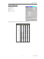
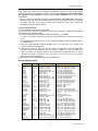
Initial maps for AHAS
An AHAS project requires initially 11 ILWIS maps to operate. These images must be created
outside of this user interface using a specialized AVHRR pre-processing package.
1. Reflectance maps in channel 1 and 2 (CH1 & CH2) non-atmospherically corrected.
• Units: reflectance: min=0 max= 1 precision= 0.001 (2 bytes)
2. Reflectance maps in channel 1 and 2 (CH1 & CH2) atmospherically corrected.
• Units: reflectance: min=0 max= 1 precision= 0.001 (2 bytes)
3. Brightness temperature for channels 3, 4 and 5
• Units: Kelvin degrees: min= 250 max=350 precision 0.1 (1 byte) for Channel 4 and 5.
• Channel 3 might have higher ranges.
• For these paper these maps are called: CH3BT, CH4BT and CH5BT
4. Solar zenith angle map
• Units: degrees: min=0 max=90 precision=0.1 (1 bytes)
5. Satellite zenith angle map
• Units: degrees: min=0 max=90 precision=0.1 (1 byte)
• For this paper this map is called: VZA
6. Solar azimuth angle map
• Units: degrees: min=0 max=360 precision=0.1 (2 bytes)
7. Satellite azimuth angle map
• Units: degrees: min=0 max=360 precision=0.1 (2 bytes)
Total 11 raster maps
• In order to reduce the amount of undefined pixels in many outputs, be certain that the initial
images are cloud free (or cloud masked), the atmosphere is clean (no smokes) and all
radiometric anomalies have been masked (fires, high reflective bodies, sun glint). To mask an
image set as undefined the anomaly pixels. See ILWIS help file: ILWIS undefined
• All maps must have a unique coordinate system and a unique georeference, otherwise it
will be impossible to operate with them.
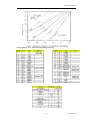
Hardware / software requirements
Operation system: Windows 95 or 98
ILWIS 2.2 software: ILWIS home page
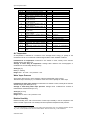
Minimum
Processor
Internal memory
HD capacity
Recommended
Pentium
8 Mb
1.2 MB
Pentium II or more
32 Mb or more
6 MB or more
Recommended adds-on
Excel-97 spreadsheet
Internet connection
ILWIS software installed in c:\ILWIS22 directory
7
AHAS User Guide
Introduction to AHAS
Installation
Download file AHAS.zip, and uncompress it in a temporal folder.
Run the setup.exe program. The installing program will setup AHAS program on your Windows
PC.
After the installation, a file named AHAS.ini is installed in your Windows directory, where paths
for running ILWIS2.2 and AHAS.exe are defined. By default the application will be installed in
c:\program files\ahas.
Uninstallation
To uninstall AHAS program, select Add/Remove Program from settings-Control Panel from the
Start menu.
AHAS User Guide
8
Introduction to AHAS
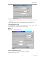
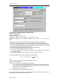
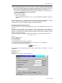
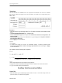
Starting AHAS
1. Click Programs-AHAS-AHAS from the Start menu. Then you will see the main application
window and the project window.
2. From AHAS File menu in the AHAS application window, select Open/New Project.
In the dialog that appears, navigate to the location of the directory that contains the project or
create a new one. An example is located in c:\rbsp\image\set3. Click 'project1' and then press
'ok' button. When the project opens, all the components contained in the project will be listed in
the project window, which enable you to add, create and explore the geographic information.
Important information
• ILWIS works independently from AHAS, so you might use it at the same time but never when
AHAS is performing a calculation. In this case, be sure that all ILWIS pixel Info box, map
windows and tables are closed.
After one image has been created in via AHAS, it will be stored in the working directory. ILWIS
treats this image as any other, so the user can apply all ILWIS functions over the created image.
9
AHAS User Guide
Introduction to AHAS
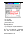
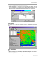
AHAS environment
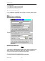
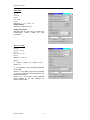
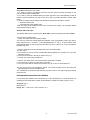
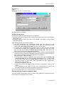
AHAS main application window
The main application window contains the tools for:
• Project management
• Image analysis
• Point interpolation
File Menu
• New project: when working in a project, select this option to initializes a new one.
• Open Project: opens an existing project.
• Close Project: closes the working project.
• Save project: saves the working project.
• Exit: exits AHAS.
• The most recently used AHAS projects will display at the botton of this menu. The user can
access the project by just clicking on them.
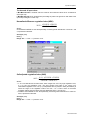
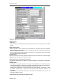
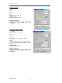
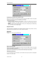
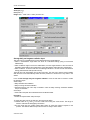
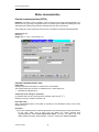
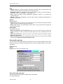
Project Menu
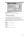
• Properties: AHAS is mainly a project-based software (one image, one site, one date). This
function opens a dialog box where the user enters relevant information to identify the
characteristics of the original NOAA image and the AHAS project itself.
• Set working directory: The user can define a directory where to store all outputs files
generated in the current AHAS project.
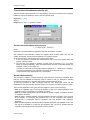
• Add images: allows the user to add ILWIS images stored externally into the current AHAS
project.
Important: to incorporate a raster image into an AHAS project, this must be an ILWIS file having
the same georeference as all other images in the project.
- First select the type of image to be incorporated by choosing the right one from the drop-down
menu.
- Then, browse in the HD or network to get the image by pressing "select image"
- Finally press "add" to add it into the system.
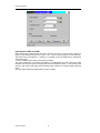
• Add image date: many outputs required the image acquisition date. The user might inter it
here. Format: mm/dd/yy
• Remove image: Allows the simple or multiple image deletion from the project.
- Select the image/s to delete from the project window.
- Select Project-remove images from the main window (alternatively select the icon in the project
window).
Note: This function removes the file from the project but it does not delete the file. It remains in
the working directory and it can be added in any moment using the function "add image". To
delete the image permanently use the your file manager software.
View
• Map window: Displays the image selected in the project window. Alternatively, select the
image an press "show map" in the project window or simply double click the map in the project
window.
Information on the functionalities of a map window in ILWIS
• Histogram: display the histogram of the image selected in the project window. Alternatively,
select the image and press "histogram" in the project window.
AHAS User Guide
10
Introduction to AHAS
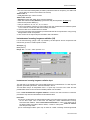
• Image properties: Selecting any image in the project window and then by applying this
function, the system displays full information of the image attributes like, coordinate system,
georeference, pixel and image sizes. This information is relevant when importing or adding
ILWIS maps into the project.
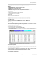
• Pixel info: Pixel info allows you to interactively inspect values in one or more raster maps.
Once this option is invoked, a "collection box" appears.
- First open one (any) AHAS map, preferably one if user interest.
- Open the pixel info box
- he user could pick one by one images from the project window, drag and drop them in the pixel
info box. By clicking on any specific pixel in the map, the pixel value and amount of pixels with
the same value is transferred and displayed for all maps listed in the pixel info box.
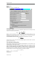
Tools
• Run Ilwis: launch the ILWIS software in case the user closes it by mistake.
• ILWIS map calculation: This option launches ILWIS map calculation functions. The user can
directly make use of ILWIS map calculation functions to create new inputs for AHAS. Once the
Map Calc menu is opened, the user is able to enter an ILWIS map calc statement, as it is
when working with ILWIS. The calculated map can be added into the current AHAS project, by
following the add image procedure explained above. The current directory for the ILWIS Map
Calculation goes to the working directory of the project file automatically when ILWIS Map
Calc opens. This function adds top flexibility to the AHAS currently programmed methods.
• Image identify: This function allows an image classification into "slices" of user selected
intervals.
• Interpolation options: Ground data from meteo-stations (point data) usually needs to be
interpolated to the entire image. In this version, AHAS system allows to simple interpolation
techniques: nearest neighborhood and moving average.
Some outputs have shortcuts (buttons) in input data dialog box to let the user fix the
interpolation method. If the shortcut does not appear in the input dialog box, it means that one
interpolation technique is preferable over the other and the user interface set it as default. In
any case the user might change the interpolation technique by accessing the interpolation
options through this menu before proceeding to the calculations.
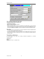
• Image preprocessing: These options are alternatives the user might choose to pre-process
the raw images before they become part of an AHAS project.
• Solar zenith angle map: This option allows the creation of a near-real time solar zenith
angle map for the georeferenced project image. One of the eleven inputs{linkID=1} of an
AHAS project is a solar zenith angle map. Usually the NOAA AVHRR pre-processing
software creates this map and in this case, the user should not use this option.
• Cloud masking techniques (not fully implemented yet)
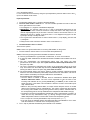
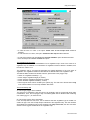
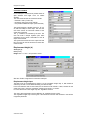
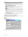
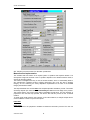
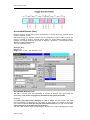
Project window
The project window is dedicated to the management of all files belonging to one unique AHAS
project. Basically it is design to:
• Keep a list of all files in the project.
• Operate as a file manager.
• From six thematic menus, the user launches output operations for all products in the AHAS.
11
AHAS User Guide
Introduction to AHAS
Thematic menus
•
•
•
•
•
•
Spectral composites: 3 submenus
Biophysical properties: 13 submenus
Climatic characteristics: 15 submenus
Water characteristics: 4 submenus
Agro-ecological: 4 submenus
Planing-allocation indicator: under construction
The "file list" indicates all file types, file names and file location in the current AHAS project.
File management
After selecting a file in the file list, the user can:
• Display the map by pressing the show map button
• Display the histogram by pressing the Histogram button.
• Delete the file from the project (It will not remove from the HD) by pressing the Delete button.
This function also accepts multi-file selection.
• Display all files in the project by pressing the display all button.
Create outputs
From the thematic oriented menus the user selects an specific output. Then all outputs of the
same type available in the project (if any), display on the file list. The others hide (press display
all to see all outputs).
To create a new output of the selected type, press the create button to initiate the
corresponding dialog box and the input procedure.
Adding images
It allows the user to add ILWIS images stored externally into the current AHAS project.
Important: to incorporate a raster image into an AHAS project, this must be an ILWIS file having
the same georeference as all other images in the project.
AHAS User Guide
12
Introduction to AHAS
- First select the type of image to be incorporated by choosing the right one from the drop-down
menu.
- Then, browse in the HD or network to get the image by pressing "select image"
- Finally press "add" to add it into the system.
Context sensitivity menu
Right click an image displayed in the project window list to access the context sensitivity menu,
which summarizes the most significant functions for images in AHAS:
• Show map:
displays the map
• Show histogram:
graph: displays the graph histogram
table: displays the table histogram
• Show pixel info:
access the cursor info function
• Image properties: Displays the characteristics of the file. The user can add comments on
the file type.
Tips and Tricks
• When performing the calculations, be sure that all ILWIS pixel Info box, map windows and
tables must be closed.
• Preferably install ILWIS in the default directory c:\ilwis22
• ILWIS works independently from AHAS, so you might use it at the same time but never when
AHAS is performing a calculation. In this case, be sure that all ILWIS pixel Info box, map
windows and tables are closed.
• After one image has been created in via AHAS, it will be stored in the working directory. ILWIS
treats this image as any other, so the user can apply all ILWIS functions over the created
image.
• Absolute maximum amount of characters allowed in an output map, table or point map is 8,
but a maximum of 7 is recommended.
• In order to reduce the amount of undefined pixels in many outputs, be certain that the image is
cloud free, the atmosphere is clean (no smokes) and all radiometric anomalies have been
masked (fires, high reflective bodies, sunglint).
• After the installation, a file named AHAS.ini is installed in your Windows directory, where paths
for running ILWIS2.2 and AHAS.exe are defined. By default the application will be installed in
c:\program files\ahas.
13
AHAS User Guide
Spectral Composites
Spectral Composites
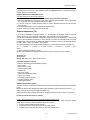
Color Composite Images
Combining 3 raster images (bands/maps) creates a color composite. One band is displayed in
shades of red, one in shades of green and one in shades of blue.
Assign channels to color bands
Assign Red, Green or Blue color to the three selected channels. The user can browse in the
system by clicking the browse button next to the filename.
By default:
Red: channel 4.
Green: channel 2.
Blue: channel 1.
Characteristics of the default configuration:
• The hottest pixels in the image (driest) will assume red colors. This way is easy to identify
sector suffering of stress.
• Well-watered healthy vegetation will assume greenish tones.
• Blue will indicate less vegetated areas not hot and water bodies.
Linear stretching
Select Linear Stretching if you want to obtain intervals of equal length (in terms of input values)
for the output colors.
Histogram equalization
Select Histogram Equalization if you want to obtain an equal number of pixels for the different
output colors.
Use intervals as Min:Max
Select this check box to specify input intervals by a minimum and maximum value of each input
map. Clear this check box to define input intervals by a percentage of pixels to be ignored on
both sides of the input map's histogram.
AHAS User Guide
14
Spectral Composites
The intervals of input values
If Min:Max intervals is checked enter the minimum and maximum values to be considered in
each input map.
If Min:Max intervals is not checked enter percentage of pixels to be ignored on both sides of the
input map's histogram in each map.
Normalized difference vegetation index (NDVI)
NDVI =
CH 2 SUR − CH 1SUR
CH 2SUR + CH 1SUR
Where:
CH1SURand CH2SUR are the atmospherically corrected ground reflectances in channel 1 and
2, expressed in decimals.
Acronym: [ndvi]
Unit: [-]
Range: Min =-1 / max = 1 / precision =0.01
Soil adjusted vegetation index (SAVI)
SAVI =
(1 + L) ⋅ (CH 2 SUR − CH 1SUR)
CH 2 SUR + CH 1SUR + L
Where:
• 'L' is a non-dimensional correction factor, which ranges from 0 for very high vegetation cover,
to 1 for very low vegetation cover. The most typically used value is 0.5, which is for
intermediate vegetation cover. The (1+L) multiplicative term is present in SAVI (and MSAVI) to
cause the range of the vegetation index to be from -1 to +1.This is done so that both
vegetation indices reduce to NDVI when the adjustment factor L goes to zero.
• CH1SUR and CH2SUR are the atmospherically corrected ground reflectances in channel 1
and 2, expressed in decimals.
Acronym: [savi]
Unit: [-]
Range: Min =-1 / max = 1 / precision =0.01
15
AHAS User Guide
Spectral Composites
Input maps for NDVI and SAVI
Green leaves have a reflectance of 20 percent or less in the 0.5 to 0.7 micron range (Channel 1:
green to red) and about 60 percent in the 0.7 to 1.3 micron range (Channel 2: near infra-red).
The value is then normalized to -1<=NDVI<=1 to partially account for differences in illumination
and surface slope.
'L' is the correction factor, being 0.5 the value by default.
The initial construction of this index was based on measurements of cotton and range grass
canopies with dark and light soil backgrounds, and the adjustment factor 'L' was found by trial
and error until a factor that gave equal vegetation index results for the dark and light soils was
found.
The user might change the default value in case is needed.
AHAS User Guide
16
Biophysical Properties
Biophysical properties
Fractional vegetation cover (vc)
Vc = ( SAVI − SAVI s ) /( SAVI d − SAVI s )
Where:
SAVI: is the SAVI value of the current pixel (SAVI map)
SAVIs is the value of SAVI for soils without vegetation selected from the SAVI image.
SAVId is the value of SAVI for dense canopies selected from the SAVI.
Acronym: [Vc]
Unit: [-]
Range: Min =0 / max = 1 / precision =0.01
Fractional vegetation cover input
SAVI: is the SAVI value of the current pixel (SAVI map)
SAVIs is the value of SAVI for soils without vegetation selected from the SAVI image.
SAVId is the value of SAVI for dense canopies selected from the SAVI.
Procedure and default values
• The user interface automatically calculates the maximum (default for SAVId) and minimum
(default for SAVIs) pixel values from the created SAVI map. The maximum and minimum value
must be entered before proceeding to calculate vc.
• If the minimum SAVI is negative means presence of water. SAVI maps are not filtered
(negatives remain). However for the calculation of the "fractional vegetation cover", it should
not be an option for the user to change the minimum SAVI value. In case the minimum SAVI is
negative, the default for "min SAVI" is changed to zero.
• The UI allows displaying the SAVI map to modify or verify these defaults. The user might
select a maximum SAVI value from the screen using pixel info and the histogram of the SAVI
map. At the same time a histogram of the SAVI could be displayed.
Leaf area index (LAI)
The LAI is the cumulative area of leaves per unit of land at nadir orientation.
17
AHAS User Guide
Biophysical Properties
Acronym: [LAI]
Unit: [-]
Range: Min =0 / max = 10 / precision =0.01
Leaf area index input
The procedure is limited to the use of the interpolation equation that is the average of many
experiences developed by several authors.
LAI = −
 c − SAVI 
1

⋅ ln 1
c3
c2


Default: c1= 0.69 c2=0.59 and c3= 0.91. The user could also select a different value from a crop
dependent list or any other value. In case of AVHRR imagery the LAI calculated following this
methodology must be taken with caution.
In case of Sahelian environment, a linear relationship was found between LAI and SAVI:
LAI =
SAVI − c1
c2
If the user enters c1 and c2 only, then the linear equation applies. If he also enters c3, then the
logarithmic expression does.
Crop reflectance coefficient (Kcr)
The Kc value is the ratio of the crop potential evapotranspiration over the reference crop
evapotranspiration, usually (alfalfa or grass).
The Kc's depends on the type of crop, meteorological conditions and according to several
authors, the driving parameters that indicates its change with time for a certain crop is the
fraction of growing degree days from planting. For certain crop type, the ground coverage
detected from RS in for of vegetation indexes gives the indication of stage development and so,
days after planting. This is the concept behind the crop reflectance coefficient.
K cr = c1 ⋅ SAVI + c2
Defaults: c1= 1.461, c2= 0.017 (wheat)
Acronym: [Kcr]
AHAS User Guide
18
Biophysical Properties
Unit: [-]
Range: Min =0 / max = 2.54 / precision =0.01
Crop reflectance coefficient input
Crop coefficients default: c1= 1.461, c2= 0.017, valid for the case of wheat.
The user could also select a different value accordingly. In case of AVHRR imagery the Kcr
calculated following this methodology must be taken with caution, in case of impure pixels.
Crop coefficient Priestley and Taylor
Definition: the ratio of crop potential evapotranspiration to the evapotranspiration of a reference
crop, usually grass or alfalfa.
Acronym: [Kc]
Unit: [-]
Range: Min =0 / max = 2.54 / precision =0.01
19
AHAS User Guide
Biophysical Properties
Crop coefficient Priestley and Taylor input
The maps required for these calculations are:
• Broadband surface albedo
• Daily incoming shortwave solar radiation
• Daily net longwave radiation
• Raster map (called "mask") indicating the irrigated and no-irrigated fields. The map must have
the same georeferencing of the other maps in the project and a domain CLASS with only two
class types: irrigated / no-irrigated. Care with the spelling, otherwise the calculation will fail.
Other inputs:
• A conversion factor for surface albedo to convert the instantaneous surface broadband albedo
in a daily average broadband albedo (default: 1.0).
• In case the user decides to apply the calculation to the irrigated areas, then the user must
enter the mask and check the "Apply mask" box. If it is not checked the calculation apply for
the entire image.
Transpiration coefficient (tc)
It is the fraction
evapotranspiration.
that
results
from
dividing
Acronym: [tc]
Unit: [-]
Range: Min =0 / max = 1 / precision =0.01
AHAS User Guide
20
unstressed
transpiration
by
potential
Biophysical Properties
Transpiration coefficient input
• A Leaf Area Index (LAI) map is required. The UI will detect one of the available in the project.
The user might browse for a LAI map or create one from this dialog box by pressing the
‘browse button’.
• The user has to define a value for c11 that varies between 0.5 and 0.8. (Default= 0.59).
Planetary broadband albedo
It is the instantaneous hemispherical planetary reflectance of shortwave radiation between
wavelengths of 0.3 and 3 µm, estimated from the visible channels.
Acronym: [rp]
Unit: [-]
Range: Min = -1 / max = 1 / precision =0.001
Planetary broadband albedo input
rp = c 4 + c5 ⋅ CH 1TOA + c 6 ⋅ CH 2TOA
According to Valiente et al. (1995)
21
AHAS User Guide
Biophysical Properties
• 'c4' (default= 0.035)
• 'c5' is a weight factor for channel 1 (default= 0.545)
• 'c6' is a weight factor for channel 2 (default= 0.32)
These coefficients can be modified by the user.
Broadband surface albedo (ro)
It is the instantaneous hemispherical surface reflectance of shortwave radiation between
wavelengths of 0.3 and 3 µm, estimated from the visible channels.
Acronym: [ro]
Unit: [-]
Range: Min = 0 / max = 1 / precision =0.001
2-ways transmittance constant method
Transmittance from stations (opened from the constant method)
Broadband surface albedo input
ro =
rp − c7
c8
According to Chen and Ohring (1984) and others.
'c7' is the offset in the relationship between broadband planetary albedo and broadband surface
albedo. (The albedo of a non-reflective body, deep sea water, appearing in the image or not.
'c8' It is the two-way transmittance of the broadband shortwave radiation.
There are two built-in procedures in the user interface;
a- The user enters the 2-way atmospheric transmittance (0.5 by default)
b- The system calculates it from ground station data from pyranometers.
AHAS User Guide
22
Biophysical Properties
a- It is the default method.
b- This method can be accessed by using the input dependency launcher button next to the 'c8'
input in the default create screen.
Input requirements
1. The planetary albedo map (rp) must be calculated already.
2. The user must decide a value for 'c7'. The user interface provides the tools to allow the
user a right selection for this value.
• The histogram of 'rp' might be calculated and displayed.
• IMPORTANT: The minimum value for the 'rp' map is automatically determined by the
system. The user must confirm the existence of deep-sea water in the image, since the
method originally applies only in this case. If the user confirms, the minimum value of 'rp' is
offered to the user as 'c7' default.. If he rejects, then 'c7' is re mapped to min(rp)/2. The user
is prompt to accept or modify this value.
• The UI gives some standard tools to select a better value: 'rp' map display, pixel info and
'rp' histogram.
• Finally the user must confirm the default or enter a new value for 'c7'.
3. The determination of the 'c8' factor:
There are two options:
Case a- there is no ground information on incoming SW radiation on the ground.
• The user enters a uniform value of 'c8' for the entire area (default=0.5).
Case b- There are ground pyranometers available in stations in the area.
a) There is ground data from a pyranometer or solarimeter, in one or more locations.
b) A new map called "instantaneous terrestrial shortwave broadband solar radiation" has to be
created.
c) The user creates/opens the meteorological station point map having the same
georeference as the other maps. Select open solarimeter station map-show button. See
also point map editor.
• The user is requested to enter/select the location of the solarimeter stations in the point
map. This is done from the ILWIS map windows by edit-edit layer-point map name. After
entering the station name in the point map, press enter to confirm.
d) The meteorological station point map is linked to a table containing meteorological data
where the user enters attributes (meteo-data) of different kind for each station. The user is
able to edit the meteodata point map and add/remove meteostations.
See ILWIS help file: ILWIS point maps
• Once the station is entered or selected, select a name/edit the attribute table: open
attribute table-show button. The user is then requested to enter the value of the
2
incoming solar radiation at the ground (column Kin_i in watt/m ) at the moment the
image was taken, in the station. This information is stored in a column of the station point
map - attribute table.
• Based on this point map attribute table, via scripts another temporal column is created
without user interaction (Column transmittance). The column contains the ratio between
the incoming solar radiation at the ground (previous column) and the extracted value of
the corresponding pixel in the map instantaneous hemispherical SW radiation map (b).
• The station point map is interpolated by the attribute column "transmittance" (invisible), to
create the one way "transmittance map" (τ). Moving average inverse distance is the
default interpolation method. To select other method see interpolation options.
• The 'c8' map is the "one way transmittance map" at the power 2. (c8 = τ2)
• If the user enter the available stations but solarimeter data is unavailable for one or more
enter the undefined "?" character in the corresponding column.
4. The 'r0' map is produced automatically since all data is now available.
23
AHAS User Guide
Biophysical Properties
Thermal infrared broadband emissivity (e0)
Thermal infrared surface emissivity (ε0) is the efficiency with which the surface emits longwave
radiation at a given temperature in the 3 to 100 min spectral range.
Acronym: [εo, ε4 or ε5]
Unit: [-]
Range: Min =0 / max = 1 / precision =0.0001
Thermal infrared broadband emissivity input
ε o = 1.0094 + 0.047 ⋅ ln( NDVI )
where
NDVI is the normalized difference vegetation map after atmospheric correction.
The procedure is fully automatic. However for negative values of NDVI (water, bare soil and
clouds), the equation cannot be solved (logarithm of a negative number).
To solve this issue the system filters some negative NDVI values:
1. It uses the equation to calculate the initial emissivity map. In this map negative NDVI will
produce undefined values.
2. The next step is the attempt to reassign a proper value of emissivity (εwater= 1) to water
bodies. According to Salisbury, 1992, wet bodies and wet bare soil can be assigned with the
emissivity of water, so, the steps are:
• Creation of a temporal emissivity map: tempemi= Iff(NDVI<0, 1, 1.0094+0.047 . ln(NDVI))
• The temporal emissivity map is filtered for emissivity values less than 0.91
• Final emissivity map= iff(tempemi<0.91,0.91,tempemi)
Narrow band emissivity
This procedure is valid for a certain wavelength range where the emissivity is calculated. Most
likely the user will estimate the emissivity maps in channel 4 and 5. It attempts to estimate
narrow band emissivity from vegetation index maps and pure emissivity values.
To redo the procedure for other wavelength range the only values that change are the
emissivities for the bare and pure vegetation pixels. The rest of the procedure remains the same.
There are four application cases, going from the simplest (1) to the most complete (4):
• Case 1: No vegetation map nor soil map is available, no idea of the spatial distribution of the
vegetation exists, no information on vegetation structures.
• Case 2: No digital vegetation/soil map is available, but analog or tabular. Information do exists
on vegetation structures.
• Case 3: There is a digital vegetation map and vegetation structure information. If the soil map
is not available, it is built from the vegetation map. The user recognizes that vegetation
heterogeneity is predominant and the vegetation map only identifies main vegetation
structures.
• Case 4: Digital vegetation maps and structure available. Digital soil map available or not. If the
soil map is not available, it is built from the vegetation map. The user is confident that the
vegetation map reproduces the heterogeneity found in the field.
AHAS User Guide
24
Biophysical Properties
Concepts and procedures
1- Determination of the NDVI based vegetation proportion.
Pv =
1 − NDVI / NDVI g
(1 − NDVI / NDVI g ) − K ⋅ (1 − NDVI / NDVI v )
K=
CH 2 SURv − CH 1SURv
CH 2 SURg − CH 1SUR g
Where:
• NDVIg and the NDVIv are the NDVI values of the user selected for pure ground and pure
vegetation pixels. The user has to enter the NDVIg and the NDVIv values.
• NDVI is the NDVI map
• 'K' is the ratio between the difference of the reflectance of the fully vegetated pixel in Channel
2 and Channel 1 by the same difference but for the bare soil pixel. It is an image constant.
• CH1SUR and CH2SUR are atmospherically corrected reflectance.
• Pv is the vegetation proportion map.
Considerations:
• NDVIg and the NDVIv are image constant values that might correspond to the minimum (nowater) and maximum NDVI in the reference image.
Vegetation proportion map
This map must is not the fractional vegetation map as was built in the "biophysical properties"
menu in the UI. In order to built the map, the user might press the input independency launcher
button.
• Before solving this map, the user must be acquainted with the theory.
• The operation triggers a procedure were the system searches for the highest and the lowest
NDVI pixel in the image. For these pixels the atmospherically corrected reflectances in
channel 1 and 2 are place in the dialog box.
• The user can display the histograms and maps in order to verify/correct the input data. If the
user wishes to change the default selected values he must enter the new column and row for
the pure vegetated and/or bare soil pixel and press <enter> to accept.
• Once the input data is fixed, the user selects a name for the output PV map and press "OK".
25
AHAS User Guide
Biophysical Properties
Vegetation proportion map input
Required maps:
• NDVI map
• CH1 and CH2 are atmospherically corrected reflectances, these are input maps to the AHAS
project.
Other required values:
• NDVIg and NDVIv are the values of the user selected for pure ground and pure vegetation
pixels. The user interface searches for the location and value of the maximum and minimum
NDVI and displays it as default.
• The user might accept/change the location of these pixels. The histogram, show map and pixel
info tools assist the user in the search.
Considerations:
NDVIg and the NDVIv are image constant values that might correspond to the minimum (nowater) and maximum NDVI in the reference image.
2- Determination of emissivities for pure pixels.
The emissivity values for the pure ground εg and pure vegetation εv pixels have to be entered by
the user.
Considerations:
• The emissivity of the pure ground can be as high as the vegetation in case that the ground is
covered with vegetation. Typical case is the fallow Savannah covered with perennial grasses.
• The values are applicable to any wavelength range selected by the user.
• For each unit considered by the user (see cases) one unique value for εg and one for εv has to
be defined. However only in case 4 the user needs to enter all these values for the
calculations.
• Alternatively some background information and tables will be available where the user can
have some reference values.
3- Determination of emissivity correction term <dεε>
AHAS User Guide
26
Biophysical Properties
Concept: <dε> is a correction for the emissivity non-linearities with NDVI. It is a function of
vegetation structure and satellite view angle.
<dε> is always a raster map. In cases 1, 2 and 3, this map assumes a constant value. This is
mainly due to lack of information from the user. In case 4, <dε> is a variable raster map.
<dεε> in the different cases:
The user is in case 1:
In this case the <dε> is only one unique value entered by the user.
The user should investigate a mean value of <dε> based on a number of observations
(vegetation and emissivities) for a reasonable number of distinct structures.
The user interface provides some assistance to the user:
• Links to global vegetation maps or other useful pages in internet, in order to define main
vegetation structures.
• A database for soil and vegetation emissivities in channel 4 and 5 to define narrow band
emissivity values for pure classes.
• A <dε> calculator: this is an specialized calculator that provides the value of <dε> based on
certain parameters entered by the user.
• Finally the user enters in the system an unique value of <dε> equal to the average of all <dε>'s
he investigated.
< dε >= dε ef = Avg (dε i )
Where:
'dεI' is calculated by each vegetation structure
The user is in case 2:
In this case the <dε> term is only one unique value entered by the user.
The user can apply the same tools available for the case 1, but the final <dε> is a
weighted mean value. The equation he might use is:
n
< dε >= dε ef = ∑ f i ⋅ dε i
i =1
Where:
'dεI' is calculated by each vegetation structure
'fI' is the weight area corresponding to each vegetation unit.
The user counts with an on-line calculator for <dε> estimates, the weighted <dε> has to be
calculated outside and is enter manually.
The user is in case 3:
In this case the <dε> term is only one unique value calculated from GIS techniques through the
user interface.
The user provides:
• The vegetation map and attributes data.
• The soil map and attributes data.
1
The operational calculation of the exact value of dε is rather complicated .
1
The user interface has to produce a series of calculations in order to produce a unique value of <dε>
I.
The UI calculates the G, F and F’ values in the attribute table from the vegetation map.
II.
A “Pt” column can be calculated from the attribute table from the vegetation map:
L2
Pt =
( S + L) 2
III.
IV.
V.
VI.
VII.
H, L, S, G, F, F’ and Pt attributes from the vegetation map are rasterized using the georeference in the system.
εv attribute from the vegetation map is rasterized using the georeference in the system.
εg attribute from the soil map is rasterized using the georeference in the system.
A “Ps” map is created as:
Ps =
VIII.
H ⋅ L ⋅ tan(VZA)
( S + L) 2
A dε map is calculated as:
27
AHAS User Guide
Biophysical Properties
So, a simplified method is proposed in this UI.
I.
The UI calculates the "F" value in the attribute table from the vegetation map.
II.
A "Pt" column can also be calculated from the attribute table from the vegetation map:
Pt =
III.
IV.
V.
VI.
L2
( S + L) 2
The "Pt" and "F" from the attribute table of the polygon map is rasterized using the
georeference in the system.
εg attribute from the soil map is rasterized using the georeference in the system.
The <dε> raster map is calculated as:
< dε >= (1 − ε g ) ⋅ ε v ⋅ F ⋅ (1 − Pt )
The average value of this map is <dε> and is used for further calculations the
calculations.
The user is in case 4:
In this case the <dε> term is a map calculated by the user using GIS techniques. Each
combination soil/vegetation might have one value of <dε>.
The procedure is exactly the same as in the previous case 3 except that the <dε> is used for
further calculations and not the averaged <dε>.
4- Calculation of the narrow band emissivity
In all cases the following equation applies.
ε = ε g ⋅ (1 − Pv ) + ε v ⋅ Pv + 4⋅ < dε > ⋅Pv ⋅ (1 − Pv )
Procedure
1- The user has to identify his emissivity application case.
2- The user must enter data that is common for all cases
Pv (Vegetation proportion map)
This map must is not the fractional vegetation map as was built in the "biophysical properties"
menu in the UI. In order to build the map, the user might press the dependency launcher
button.
• The operation triggers a procedure were the system searches for the highest and the lowest
NDVI pixel in the image. For these pixels the atmospherically corrected reflectances in
channel 1 and 2 are place in the dialog box.
• The user can display the histograms and maps in order to verify/correct the input data. If the
user wishes to change the default-selected values he must enter the new column and row for
the pure vegetated and/or bare soil pixel and press <enter> to accept.
• Once the input data is fixed, the user selects a name for the output PV map and press "OK".
• By default the Create narrow band emissivity dialog box opens for cases 1 and 2. In case the
user is in cases 3 or 4 (vegetation structure map is available), select: "Vegetation structure
map" in the "Option on method sector.
• Once emissivity data for cases 1 to 4 are solved, the final narrow band map calculates by
pressing the OK button.
Cases 1 or 2
For cases 1 or 2, the first choice is to use the in-built <de> calculator or not.
1- The user requires the use of the <de> calculator.
dε = (1 − εg ) ⋅ ε v ⋅ F ⋅ [1 − ( Pt + Ps)] + [(1 − ε v ) ⋅ ε g ⋅ G + (1 − ε v ) ⋅ ε v ⋅ F ' ] ⋅ Ps
AHAS User Guide
28
Biophysical Properties
1- It is the option by default. The ‘Would you like to apply the <de> calculator’ option must
be checked.
2- If the user is in case 1- then select: Average <de> emissivity value in the Option on <de>
calculator. The weight column must be kept empty.
3- If the user is in case 2- then select: Weighted <de> mean value in the Option on <de>
calculator. The weight column indicates the proportion (decimal) of each vegetation structure
in the region. The weight is a multiplicative factor between 0 and 1. The user must verify that
the summation of the weight column equals 1.
4- The user must enter the vegetation structure data (height, spacing and breadth) for each
vegetation type selected in the region. Each line in the calculator corresponds to one unique
vegetation structure. The user has to enter all recognizable vegetation types and emissivities
before pressing the "Apply" button.
5- The user must enter the emissivity of a pure bare soil and pure vegetation in each selected
structure, for the spectral range he/she wants to work.
6- Finally the user "Apply" the calculation. The final <de> result (weighted or averaged,
depending on the selection) is place in the corresponding dialog box ready for further
calculations. The individual <de> results are place in the last column (scroll to see it).
7- The user need to enter the Pv (Vegetation proportion map).
8- Select a name for the output map and press 'OK'.
Additional features in the <de> calculator
• Each line in the <de> calculator corresponds to one unique type of vegetation structure that
has been identified by the user for the region under study. A collection of vegetation structures
(several lines in the <de> calculator) defines as it best the different types of vegetation
structures available in the area. This information is distinct for each region and might be
applied to several images of the same region. Then, once the table is completed, the user has
29
AHAS User Guide
Biophysical Properties
the option to "save" the input vegetation structure data and "load" it in any occasion.
• Any line (a vegetation structure description) can be selected for deletion by pressing the cell to
thee right of the "height" column in the corresponding line. The marker arrow activates and the
line is selected. To delete it, press the "delete" button.
• Once a line is selected, the scrolling arrows below the <de> input table could be used to go up
and down. Alternatively, just select other column using the mouse.
• If anything goes wrong in the <de> calculator, press the "Refresh" button, to reset the
calculator. Data is not lost in the operation.
2- The user does not use the in-built calculator.
1- The Would you like to apply the <de> calculator option must be unchecked.
2- The user calculates the one unique overall <de> value that goes as input in the corresponding
cell. He decides then the procedure to weight the value.
3- The user enters one overall emissivity value for a fully vegetated pixel and one for the fully
bare soil pixel.
4- The user need to enter the Pv (Vegetation proportion map).
5- Select a name for the output map and press 'OK'.
Cases 3 or 4
These options requires the existence of a polygon maps describing the vegetation structure and
soil types. This last one is optional.
AHAS User Guide
30
Biophysical Properties
• In case the user is in case 3, the option: Create <de> as one unique value should be
selected.
• In case the user is in case 4, the option: Create the <de> map should be selected.
• In case a soil polygon map is available the soil map available? option should be checked.
• If the soil map is not available uncheck this option.
The vegetation structure map
The vegetation structure is a reclassification from a vegetation map in most of the cases. If no
vegetation map is available or no information of vegetation structure classes is available, then
the user is in cases 1 or 2.
The vegetation map is a polygon file describing the spatial distribution of the main types of
vegetation. The vegetation structure is described in an attribute table of the vegetation map.
The attribute table contains four attribute columns, plus the link to the polygon map:
• column ev: Vegetation emissivity εv [-].
• column height: vegetation height (H, meters)
• column spacing: vegetation separation (S, meters)
• column breadth: vegetation breadth (L, meters)
• There might be other column created by the system (eg). The user has to fill this column only
in the case that there is not soil map available. See below.
The soil emissivity map
A- The soil type polygon file is available
The user has to reclassify the soil map into an soil emissivity map for the spectral range under
consideration. Then, the soil polygon map is needed together with its attribute table containing
one column [eg] for εg for each soil unit.
B- The soil type polygon file is unavailable
If the soil map does not exist, then, the UI assumes that each vegetation type is located in a
certain soil type. Then the soil map shape is identical to the vegetation map. The user interface
will reclassify the vegetation map into the emissivity map. Only in this case, the user must enter
another column (eg) as an attribute for the vegetation map.
31
AHAS User Guide
Biophysical Properties
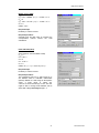
<dεε> calculator (spreadsheet)
If the user is in cases 1 or 2 he or she has to decide a unique value of <dε> for the calculations.
A "calculation box" is designed to assist in this purpose.
There are 2 version of the <de> calculator: online and spreadsheet. The on-line calculator is
designed for map production. The spreadsheet (see helpfile) is designed for both map
production and training.
Exclusive input and outputs for spreadsheet are in blue.
The inputs boxes are:
• H=height [m]
• S=spacing [m]
• L=breadth [m]
• Ev
• Eg
• Satellite view angle Ψ [°]
The output boxes are related to vegetation structure and the <dεε> term:
Percentage of top vegetation: L2/(L+S)2 rounded to 1 decimal.
Percentage of side vegetation: H*L*TAN(Ψ)/(S+L)2 [Ψ is the satellite zenith angle]
Percentage of ground vegetation: (1-Pt-Ps)
deexact: (1-eg)*ev*F*Pg+[(1-ev)*eg*G+(1-ev)*ev*F']*Ps
demax: (1-eg)*ev*F*(1-Pt) (weighted or not)
eo: ev*Pt+ev*Ps+eg*Pg
e: eo+deexact
deapprox: 4*<de>*(Pt+Ps)*(1-Pt-Ps)
eapprox: ev*(Pt+Ps)+eg*Pg+deapprox
e-eapprox: this difference to check the accuracy of the approximate model.
Online <de> calculator
1- If the user is in case 1- then select: Average <de> emissivity value in the Option on <de>
calculator. The weight column must be kept empty.
2- If the user is in case 2- then select: Weighted <de> mean value in the Option on <de>
calculator. The weight column indicates the proportion (decimal) of each vegetation structure
in the region. The weight is a multiplicative factor between 0 and 1. The user must verify that
the summation of the weight column equals 1.
3- The user must enter the vegetation structure data (height, spacing and breadth) for each
vegetation type selected in the region. Each line in the calculator corresponds to one unique
vegetation structure. The user has to enter all recognizable vegetation types and emissivities
before pressing the "Apply" button.
4- The user must enter the emissivity of a pure bare soil and pure vegetation in each selected
structure, for the spectral range he/she wants to work.
5- Finally the user "Apply" the calculation. The final <de> result (weighted or averaged,
depending on the selection) is place in the corresponding dialog box ready for further
calculations. The individual <de> results are place in the last column (scroll to see it).
Additional features in the <de> calculator
• Each line in the <de> calculator corresponds to one unique type of vegetation structure that
has been identified by the user for the region under study. A collection of vegetation structures
(several lines in the <de> calculator) defines as it best the different types of vegetation
structures available in the area. This information is distinct for each region and might be
applied to several images of the same region. Then, once the table is complete, the user has
the option to "save" the input vegetation structure data and "load" it in any occasion.
• Any line (a vegetation structure description) can be selected for deletion by pressing the cell to
thee right of the "height" column in the corresponding line. The marker arrow activates and the
line is selected. To delete it press the "delete" button.
• Once a line is selected, the scrolling arrows below the <de> input table could be used to go up
and down. Alternatively, just select other column using the mouse.
AHAS User Guide
32
Biophysical Properties
If anything goes wrong in the <de> calculator, press the "Refresh" button, to reset the calculator.
Data is not lost in the operation.
Options when <de> calculator is off
The user does not use the in-built calculator.
1- The Would you like to apply the <de> calculator option must be unchecked.
2- The user calculates the one unique overall <de> value that goes as input in the corresponding
cell. He decides then the procedure to weight the value.
3- The user enters one overall emissivity value for a fully vegetated pixel and one for the fully
bare soil pixel.
4- The user need to enter the Pv (Vegetation proportion map).
5- Select a name for the output map and press 'OK'.
Surface temperature (To)
It is the skin temperature of the land surface, i.e., the kinematic temperature of the soil plus the
canopy surface (or, in the absence of vegetation, the temperature of the soil surface).
The surface temperature retrieved from NOAA mostly uses a linear combination of the thermal
channels and the different emissivity in both channel to produce an atmospherically corrected
thermal image. The procedure is called Split Window Technique. There are several approaches
for SWT, some of them are treated in this software.
The general equation for the split window technique for a 2 thermal channel can be written as:
To = c 4 ^ 2 ⋅ CH 4 BT 2 + c 4 ⋅ CH 4 BT + c 45 ⋅ CH 4 BT ⋅ CH 5 BT + c5 ⋅ CH 5 BT + c5^ 2 ⋅ CH 5BT 2 + offset
where:
'To' is the surface temperature in Kelvin.
CH4BT and CH5BT are the brightness temperature maps for channel 4 and 5 in Kelvin.
Acronym: [To]
Unit: [Kelvin]
Range: Min =250 / max = 350 / precision =0.01
Procedure available in the UI:
• SST (no emissivity) [Coll and Caselles (1997)]
• Price (1984)
• Becker and Li (1990)
• Prata and Platt (1991)
• Vidal (1991)
• Kerr et al. (1992)
• Ottle and Vidal-Madjar (1992)
• Ulivieri el al. (1992)
• University of Valencia (1995)
• Coll and Caselles (1997)
• Customized method
Surface temperature input
The user interface provides several well-known methods to calculate Land Surface Temperature
(LST).
Most of the land surface temperature SWT require emissivity maps for channels 4 and 5 (ε4, ε5).
Other methods need the percentage of vegetation 'Pv'.
Others assume image constant values for the image like total water vapor column 'w' (gr/cm2).
In the user interface there are 2 choices:
Case 1: The user interface does no assist the creation of these maps:
In this case, the additional maps have to be entered by the user. They might be created
externally to the system and incorporated during the process:
1. The user needs to add the external maps.
2. The UI asks for the maps required for the selected method.
3. The UI let the user browse the HD/net to enter the external maps.
33
AHAS User Guide
Biophysical Properties
4. Pressing “OK” performs the calculations.
Case 2: The user interface does assist the creation of the additional maps required by the
standard methods.
1. The user selects a method for the calculation of the LST.
2. The UI asks for the maps required for the selected method.
3. If the maps do not exist, the UI guides to alternative methods to allow the creation of these
maps and then can back to this input screen to proceed the calculations.
4. Pressing “OK” performs the calculations
Available methods
For all methods:
ε4= the emissivity map in for channel 4 wavelength range
ε5= the emissivity map in for channel 5 wavelength range
AVE=ε= (ε4 + ε5) / 2 The average emissivity map for channels 4 and 5.
DE=∆ε= ε4 - ε5 The difference emissivity maps between channel 4 and 5.
Default method: Custom SST (no emissivity) [Coll and Caselles (1997)]
No emissivity maps required. This method
assumes the emitter is water.
No emissivity map is required. Care! the equation
is an approximation. It is only accurate in case of
Sea surface temperature.]
C4^2= 0.39
C4= 2.34
C45= -0.78
C5= -1.34
C5^2= 0.39
Offset= 0.56
Price (1984)
C4^2= 0
C4= [4.33 . (5.5 - ε4) / 4.5]
C45= 0
C5= [-3.33 . (5.5 - ε4) / 4.5 – 0.75 . ∆ε]
C5^2= 0
Offset= 0
Required maps:
Emissivity in channel 4 and 5
Required procedure:
Calculate AVE and DE maps by pressing the
correspondent
buttons
before
the
final
calculations.
AHAS User Guide
34
Biophysical Properties
Becker and Li (1990)
C4^2= 0
2
C4= 3.63 + 2.06808 . (1-ε) / ε + 18.924 . ∆ε / ε
C45= 0
2
C5= -2.63 – 1.91192 . (1-ε) / ε - 19.406 . ∆ε / ε
C5^2= 0
Offset= 1.274
Required maps:
Emissivity in channel 4 and 5
Required procedure:
Calculate AVE and DE maps by pressing the
correspondent
buttons
before
the
final
calculations.
Prata and Platt (1991):
Semi-empirical, uses a radiative model)
C4^2= 0
C4= 3.46 / ε4
C45= 0
C5= - 2.46 / ε5
C5^2= 0
Offset= 40 . (1 - ε4) / ε4+273.15*(1-c4-c5)
Required maps:
Emissivity in channel 4 and 5
Required procedure:
The constants a=3.46 for C4 and b=2.46 for C5
are defaults valid for Australian radiosondes
(authors). Based on a wide range of atmospheric
cases, a wider range of values are:
3.46<=a<=4.513 and 2.46<=|b|<=3.513. The user
might be able to change these defaults, but be
aware that in any case always a = |b| + 1
35
AHAS User Guide
Biophysical Properties
Vidal (1991)
C4^2= 0
C4= 3.78
C45= 0
C5= - 2.78
C5^2= 0
Offset= 50 . (1 - ε) / ε - 300 . ∆ε / ε
Required maps:
Emissivity in channel 4 and 5
Required procedure:
Calculate AVE and DE maps by pressing the
correspondent
buttons
before
the
final
calculations.
Kerr et al. (1992)
C4^2= 0
C4= 0.5 . Pv + 3.1
C45= 0
C5= - 0.5 . Pv – 2.1
C5^2= 0
Offset= 3.1 – 5.5 . Pv
Where:
Pv = (NDVI – NDVIbare
NDVIbare soil)
soil)
/ (NDVIfull
vegetation
–
Pv is a vegetation cover percentage map based
on the NDVI.
NDVIbare soil is the NDVI of the bare soil selected
by the user. (Default: the minimum NDVI from all
positive NDVI values)
NDVIfull vegetation is the NDVI of fully vegetated
pixels selected by the user. (Default: the
maximum NDVI value.
AHAS User Guide
36
Biophysical Properties
Ottle and Vidal-Madjar (1992)
C4^2= 0
C4= user entered
C45= 0
C5= user entered
C5^2= 0
Offset= user entered
The constants could be obtained by interpolation in the following table:
Coefficients for Ottle and Vidal_Madjar '92
Sat. scan angle
0
9
16
23
32
38
44
48
53
0
53
0
53
0
53
0
53
0
53
0
53
e4
e5
offset
c4
c5
1
1 0.858 3.218 -2.218
1
1 0.854 3.225 -2.225
1
1 0.833 3.23 -2.231
1
1 0.852 3.258 -2.258
1
1
0.88 3.289 -2.29
1
1 0.924 3.328 -2.329
1
1 0.928 3.372 -2.372
1
1
0.91 3.409 -2.41
1
1 0.929 3.468 -2.469
0.98 0.98 -0.403 3.219 -2.211
0.98 0.98 -0.418 3.506 -2.499
0.96 0.96 -1.687 3.213 -2.197
0.96 0.96 -1.761 3.487 -2.471
0.94 0.94 -2.889 3.214 -2.19
0.94 0.94 -3.151 3.524 -2.499
0.98 0.985 -0.502 3.023 -2.013
0.98 0.985 -0.515 3.349 -2.339
0.96 0.98 -2.186 2.444 -1.42
0.96 0.98 -2.239 2.83 -1.804
0.98
1 -1.301 2.51 -1.492
0.98
1 -1.368 2.901 -1.881
37
AHAS User Guide
Biophysical Properties
Ulivieri el al. (1992)
C4^2= 0
C4= 2.8
C45= 0
C5= -1.8
C5^2= 0
Offset= 48 . (1 - ε) – 75 . ∆ε
Required maps:
Emissivity in channel 4 and 5
Required procedure:
Calculate AVE and DE maps by pressing the
correspondent
buttons
before
the
final
calculations.
University of Valencia (1995)
C4^2= 0.58
C4= 2 - ∆ε . (0.1 . w + 1.118)
C45= -1.16
C5= -1
C5^2= 0.58
Offset= 40.51 – 40 . ε + (68 . w + 163) . ∆ε
Where:
'w' a value that represents the total water vapor
2
column in the atmospheric profile gr/cm (usually
between 0 to 6)
Required maps:
Emissivity in channel 4 and 5
Required procedure:
Calculate AVE and DE maps by pressing the
correspondent
buttons
before
the
final
calculations
AHAS User Guide
38
Biophysical Properties
Coll and Caselles (1997)
C4^2= 0.39
C4= 2.34
C45= -0.78
C5= -1.34
C5^2= 0.39
Offset= 0.56 + α (1-ε) - β ∆ε
Where:
'α' and 'β' are value that depend on the total
water vapor column in the atmospheric profile
2
gr/cm (usually between 0 to 6)
Select the total water vapor in the 'x' axis and
read 'α' and 'β' in the ordinates.
Required maps:
Emissivity in channel 4 and 5
Required procedure:
Calculate AVE and DE maps by pressing the
correspondent
buttons
before
the
final
calculations.
Alpha and Beta (Caselles and Coll, 1997)
160
140
alpha
120
beta
100
80
60
40
20
0
0
1
2
3
4
5
water vapor (gr . cm-1)
39
AHAS User Guide
Biophysical Properties
Customized method
It is an attempt to customize all possible cases of
Split windows that might occur for NOAA
AVHRR.
The user should be able to browse and locate:
• Channel 4 and 5 (T4 and T5)
• emissivity maps 4 and 5 (E4 and E5)
• two possible "additional maps" (AD1 and AD2)
The system assigns a variable name (T4, T5, e4,
e5, AD1 and AD2) to these maps. The user can
use these names as shortcuts instead of the
entire path of the files.
The 'cI' constants, are entered by the user. The
user can enter a simple equation (four basic
operations) as any linear combination of the all
maps and constants.
The system also knows two more maps AVE and
DE. The user can use the shortcuts for these two
names as well.
Displacement height (d)
Acronym: [d]
Unit: [meter]
Range: Min = 0 / max = 30 / precision =0.001
See also: Surface roughness for momentum transport
Displacement height input
The basic map for the displacement height 'd' is the vegetation height map 'h', that should be
entered by the user. The UI allows browsing to locate the map.
In the most extreme case of lack of data, the UI allows to enter a fixed 'h' value, constant for the
entire area in the 'h' map box. Instead of "browsing" just enter 'h' in meters.
For more references to the height map see: vegetation structure.
The user is also requested to select a different 'cd', a default of 20.6 is given.
The vegetation height map must be given. See Interaction with the user interface in the surface
roughness parameter.
AHAS User Guide
40
Biophysical Properties
Surface roughness for momentum transport (zo)
It is a fraction of the crop height used as a
physical reference for momentum and heat flux
calculations
For an open site, the wind profile can be
described for a logarithmic law:
u(z) =A . ln(z) + B
'B', is usually replaced by 'A . ln (zo)' where 'zo' is
a small value of 'z' for which the previous
equation predicts u(z)= 0. Then,
u(z) = A . ln(z / zo)
'zo' is called aerodynamic roughness of the surface..
Acronym: [zo]
Unit: [meter]
Range: Min =0 / max = 0.2 / precision =0.00001
See: displacement height 'd'
Surface roughness input
The basic input for the roughness length for momentum transport as described in the roughness
length theory is three maps:
• LAI
• The vegetation height map
• The displacement height map
The UI allows an extreme simplification if a vegetation height map 'h' is unknown. The map could
be replaced by a constant representing a uniform height in the area in [m], despite the error in
the calculations. See also: vegetation structure.
Three coefficients are also required:
• Unobstructed bare soil drag: Cs Default= 0.003
41
AHAS User Guide
Biophysical Properties
• Overstore drag coefficient: Cr Default= 0.35
• Constant Cw: Default= 2
About these coefficients the Author says:
• The value of 'Cs' es equal to (u*/uh)^2. The original value of Raupach, 1992 is Cs= 0.003.
This value should be suitable for row crop and tiger-bush sites where the ground is bare soil. It
is probably too small for Savannah sites where the ground is grassed beneath the shrubs.
Using the previous equation different values of Cs can be calculated from data available in the
literature: for long grass and heather Cs= 0.018. Because of the Savannah grass is rather
sparse, an intermediate Cs= 0.010 is adopted for this type of vegetation.
• In Raupach, 1992, an overstorey drag coefficient Cr= 0.3 is chosen for bush-like obstacles;
this value is between 0.25 (vertical axis cylinders) and 0.4 (cubes) (see vegetation structure).
Values between 0.25 to 0.8 were tested. The optimized value for a very wide range of
vegetation varying from sparse to dense was 0.35.
• The Cw constant to be found from empirical data. A value of Cw equal to 2 was adopted by
the author since fits the value of the vegetation influence function of unstability.
Other coefficients involved in the method are:
• cd (default: 0.6) tested range 0.3 to 1.2.
• c1 (default: 0.37) seems adequate for cylinder type of vegetation (b/h=1) for higher b/h ratios,
larger c1 might be . Tested range -5 to 1.
Surface roughness and displacement height values
zo [m]
0.0002
0.0024
0.03
0.055
0.1
0.2
0.4
0.8
1.6
Landscape Type
Water surface
Completely open terrain with a smooth surface, e.g. concrete
runways in airports, mowed grass, etc.
Open agricultural area without fences and hedgerows and very
scattered buildings. Only softly rounded hills
Agricultural land with some houses and 8 meter tall sheltering
hedgerows with a distance of approx. 1250 meters
Agricultural land with some houses and 8 meter tall sheltering
hedgerows with a distance of approx. 500 meters
Agricultural land with many houses, shrubs and plants, or 8 meter
tall sheltering hedgerows with a distance of approx. 250 meters
Villages, small towns, agricultural land with many or tall sheltering
hedgerows, forests and very rough and uneven terrain
Larger cities with tall buildings
Very large cities with tall buildings and skyscrapers
Source: Wind Power Denmark
AHAS User Guide
42
Biophysical Properties
Source:Weiringa, 1977: 43 and 1980:967 (WMO permission)
43
AHAS User Guide
Biophysical Properties
Type
savannah 1
savannah 2
savannah 3
savannah 4
savannah 5
Tiger-bush 1
Tiger-bush 2
H[m]
2.3
8
9.5
2.3
2.5
4
4
L[m]
3.5
2
2
3
3
20
20
S[m]
5
20
10
3.4
6.6
40
40
LAI
0.64
0.08
0.38
1.2
0.34
0.1
0.1
Zom [m]
0.44
0.4
0.9
0.17
0.25
0.44
0.15
d [m]
1.8
4.8
7.1
0.93
1.5
2
3.7
Vineyard 1
Vineyard 2
Cotton 1
Cotton 2
Vineyard 3
Vineyard 4
Vineyard 5
Orchards 1
Orchards 2
0.9
0.9
0.49
0.38
1.5
1.5
2
3.7
3.7
0.7
0.9
0.25
0.3
0.3
0.3
1
4
4
1.5/5
2.5
1/0.5
1
1.75
1.75
2
7.3
7.3
0.08
0.26
0.38
0.2
0.3
0.3
1
0.56
0.56
0.095
0.08
0.066
0.16
0.55
0.2
0.25
0.23
1.22
0
0.31
0.31
0.1
0
0.75
1.4
0.92
0.92
Fractional Photosynthetically Active Radiation (fPAR)
Photosynthetically active radiation (PAR) describes the solar radiation available for
photosynthesis.
The fraction of solar radiation absorbed by chlorophyll pigments (fPAR) describes the energy
related to carbon dioxide assimilation and is derived from PAR absorbed by canopy divided by
the PAR available from solar radiation.
Acronym: [fpar]
Unit: [-]
Range: Min =0 / max = 1 / precision =0.01
Fractional Photosynthetically Active Radiation input
The procedure attempted in this interface follows the model explained by Asrar G. Mynenei R.B.,
Choudhury B.J., 1992, where fPAR is related to NDVI. It is strongly recommended to read the
corresponding article to verify the applicability of the default gain and offset.
fpar = offset + gain ⋅ NDVI
where:
NDVI is the normalized vegetation index map.
Defaults: Gain: 1.2222. Offset: -0.1914 (both changeable by the user).
AHAS User Guide
44
Climatic Characteristics
Climatic Characteristics
Daily terrestrial solar radiation (K↓dayexo)
The horizontal integrated daily value of the terrestrial solar radiation over all wavelengths.
Acronym: [K↓exoday]
Unit: [megajoules m-2 day-1]
Range: Min = 0 / max = 70 / precision =0.001
Daily terrestrial solar radiation input (Kday)
Since the user interface has a simple and accurate in-built solar radiation model, the only data
required by the user is the date for the calculation.
The other data required (position on Earth) is read by the system from the lat-long coordinates
assigned to the image selected by the user (the solar zenith angle map by default).
Average daily incoming shortwave radiation (K↓day)
The horizontal integrated daily value of the solar radiation over all wavelengths reaching the
ground.
Acronym: [K↓day]
Unit: [watt m-2]
Range: Min = 0 / max = 1400 / precision =0.1
Note: The total solar energy reaching the ground in 24 hs (cumulative) it would be in [megajoules
-2
-1
-2
m day ]. To obtain [watt m ] multiply by 11.5741.
45
AHAS User Guide
Climatic Characteristics
Average daily incoming shortwave radiation input
Useful unit equivalences:
1 Joule = 1 watt * sec
Instantaneous radiation = [watt * m^-2]
Solar energy = radiation * time = [watt * sec * m^-2] = [Joule * m^-2]
Average solar radiation in 24 hs = radiation * daytime / 24 hs = [Joule * m^2 / 24 hs] = [watt *
m^2]
The final (K↓day) map has to be evaluated from ground data measured in meteostations:
• “First class” meteostation might have this value as a standard reading (using solarimeters).
• Second class meteostation might not have the solarimeters, but some approximation to the
real value is possible if these stations have periheliometers (measuring hours of sunshine).
First class stations might also have periheliometers.
Then, the final map is a special interpolation from a point map containing:
• K↓day data from first class station entered by the user.
• K↓day data calculated from sunshine hour’s data using a simple model derived for
meteorology purposes.
• Other stations might exist, but do not add information to obtain the final map.
The following equation relates hours of sunshine and daily radiation:


n
K ↓ day = 11.5741 ⋅  a s + bs ⋅  ⋅ K ↓ exo
day 
N


where:
exo
-2
-1
'K↓day '= the daily terrestrial solar radiation (megajoules m day ).
'n/N' is the sunshine fraction [-]
'as' and 'bs' are constants to be evaluated at ground stations.
as + bs= total fraction of terrestrial radiation reaching the ground in a complete clear day.
'as' is the fraction of terrestrial radiation reaching the ground in a complete overcast day.
'as' and 'bs' have to be calculated at any station.
Default values: 'as'= 0.25; 'bs'= 0.5
-2
'K↓day'= the daily average ground solar radiation (watt m ).
If one station has both solarimeter and periheliometer data, the calculation for the station is
performed with the solarimeter data, ignoring the rest.
AHAS User Guide
46
Climatic Characteristics
Procedure: Basically the user needs:
1- To create (or open) a point station map where the user is able to position the station on the
map and add a name or identification.
2- To create (or open) an attribute table for the point map where the UI automatically creates all
relevant columns needed for the user to enter K↓day data, by pressing the button “column table
button”
3- Create or identify maps needed for the calculations if periheliometer data is needed:
• Sunshine fraction map.
• Terrestrial daily solar radiation map.
These two maps can be created from this menu or browse in the system. The UI assigns default
maps already existing in the UI.
Attribute table data input:
The attribute table opens by selecting the "Show table" option and pressing the button "Show".
There are three possible cases:
• Case I- The station has daily solarimeter data.
The user only enters the average daily solar radiation in the corresponding column (Kin_da) for
-2
-2
-1
these stations (care: it is [watt m ] and not [Megajoules m day ]). If these stations have
periheliometer data, the user might enter this data type (as in case II), but for this calculations
this data is ignored.
• Case II- The station has only periheliometer (hours of sunshine) data.
The user enters:
a- The constant 'as' and 'bs' for the corresponding stations (default 'as'= 0.25 and 'bs'= 0.5) in the
respective columns.
b- The hours of sunshine in this day in column Sun_hs_d
c- The (Kin_da) column stays undefined '?'
• Case III- The station does not have information related to this variable.
a- The user does not enter any information in this case.
b- The user checks that the values of the columns Kin_da, 'as' and 'bs' are undefined '?'.
The user should verify the interpolation method. The moving average inverse will seems the
most appropriate to smooth out differences.
The calculations are performed after selecting a proper name for the output map and pressing
the button 'OK'.
Instantaneous terrestrial solar radiation
It is the total solar radiation that reaches the top of the atmosphere at a certain moment in a
predefined horizontal position on Earth. Solar radiation is usually call "visible" (range 0-3 µm)
Acronym: [K↓exo]
Unit: [watt m-2]
Range: Min = -1400 / max = 1400 / precision =0.1
47
AHAS User Guide
Climatic Characteristics
Instantaneous terrestrial solar radiation input
Since the user interface has a simple and accurate in-built solar radiation model, the only data
required to be entered by the user is the date for the calculation.
The other data required is:
• Position on Earth (coordinate of the pixels): is read by the system from the lat-long
coordinates assigned to the image selected by the user (the solar zenith angle map by
default).
• Position of the Sun (solar zenith angle): is read by the corresponding file created during
the preprocessing of the AVHRR imagery.
Daytime duration
This map shows the total duration of the daytime (sunrise to sunset) at any location. The map
indicates then the total sunshine hours in case of a perfect clear day.
Acronym: [N]
Unit: [hours]
Range: Min = 0 / max = 25.4 / precision =0.01
Daytime duration input
Since the user interface has a simple and accurate in-built solar radiation model, the only data
required is the date for the calculation.
The other data required (position on Earth) is read by the system from the lat-long coordinates
assigned to the image selected by the user (the solar zenith angle map by default).
Sunshine fraction (cc)
It is the ratio between the real number of clear sunshine hours per day and the total daytime
duration for an specific date.
AHAS User Guide
48
Climatic Characteristics
Acronym: [cc]
Unit: [-]
Range: Min =0 / max = 1 / precision =0.01
See: Potential hours of sunshine
Sunshine fraction input
Daily sunshine fraction in the user interface can be entered by:
• importing to the project an external daily sunshine fraction map having the same georeference
that the other maps.
• Calculating sunshine fraction point data in the available meteostations, using available
interpolation methods.
In the second case, the user proceeds as follows:
a) The user creates/opens the meteorological station point map having the same
georeference as the other maps. This is done from the dialog box create daily sunshine
fraction. Select show station-show button. See also point map editor.
• In case the station map already exists but stations have to be added, the user is requested
to enter/select the location of the periheliometer stations in the point map. This is done
from the ILWIS map windows by edit-edit layer-point map name. After entering the
station name in the point map, press enter to confirm.
b) The meteorological station point map is linked to a table containing meteorological data
where the user enters attributes (meteo-data) of different kind for each station. The user is
able to edit the meteodata point map and add/remove meteostations.
See ILWIS help file: ILWIS point maps
• Once the station is entered or selected, edit the attribute table: select show table- and
press show button. The user enters the hours of sunshine (Sun_hs_d) at the ground
(in hours) that correspond to the available stations and press "enter" to confirm. This
information is stored in an appropriate column of the station point map - attribute table.
When finished, close the table.
• To initiate the calculations, press OK.
• A raster map showing the potential hours of sunshine is automatically created by the
system.
• The UI calculates at each station the ratio real to potential hours of sunshine and
interpolates the point map using an interpolation method selected by the user.
c) The map sunshine fraction map is produced with the available data.
Average daily net longwave radiation (Lday)
This map evaluates the significant change of radiant energy between the atmosphere and the
earth's surface in the longwave range 3-100 µm.
49
AHAS User Guide
Climatic Characteristics
Acronym: [Lday]
Unit: [watt m-2]
Range: Min = -1000 / max = 1000 / precision =0.1
Average daily net longwave radiation input
This map has to be evaluated from ground data measured in meteostations.
• Class 1 meteostations might have this value as a standard reading (using in-out thermal
radiometers).
• Class 2 stations might not have the radiometers, but some approximation to the real value is
possible if these stations have solarimeters. First class stations might also have solarimeters.
• Class 3 stations. A less accurate but still valid approximation is for the second class stations
having periheliometer data (sunshine hours).
The final map is an interpolation from a Lday point map. The user has to enter the best possible
data and the UI will automatically select the best procedure to achieve the Lday value in the
station.
In the "create average daily net longwave radiation" menu the user has to browse or create
the following maps:
Raster maps:
• Daily terrestrial solar radiation.
• Daily incoming shortwave radiation
• Sunshine fraction map. This map is needed in case the daily incoming shortwave radiation
map is not available.
Point maps:
• Point station map with the meteostations and its attribute table.
Procedure:
1- Select all required raster and point maps
To create the Lday map for the first time, the user has to define:
• A default value for 'ae' and 'be' from the create menu using the scroll arrows. The range of
values is restricted to bibliography information.
• The user must 'click' the ‘create column table’ button to create the columns requires for the
process. The attribute table will open and the user is ready to enter values.
AHAS User Guide
50
Climatic Characteristics
• The user enters the following data per station (underlined if data is compulsory, the station will
not be taken into account if this data is not entered).
Station class 1:
• Lnet_da [watt/m^2] in case it is known.
Station class 2 and 3:
• Ed mean average daily water vapor pressure [millibars].
• Mean RH relative humidity RHmean [%] and mean daily air temperature Ta mean [°C].
• Minimum temperature Tmin [°C].
• Verify he values for 'ae', 'be', 'as', 'bs', 'ac' and 'bc'.
• If some of the data is unknown for some stations, the user should enter the undefined symbol
'?' the UI will not consider the data and eventually, the station.
2- Close the table once all data has been verified.
3- The user might select the interpolation procedure that best fits his requirements. Using moving
average better results are expected.
4- Give a name for the output map and click OK to start calculations.
Instantaneous incoming longwave radiation (L↓)
It is the thermal energy (range 3-100 µm) emitted by the atmosphere and its components that
reaches the ground in a certain specific moment.
Acronym: [L↓]
Unit: [watt m-2]
Range: Min = 0 / max = 1000 / precision =0.1
Instantaneous incoming longwave radiation input
This map has to be evaluated from ground data measured in meteostations. For clear days the
approach presented by Brutsaert, 1975 was selected in this UI.
The final raster map is an interpolation from a L↓ point map. The user has to enter the best
possible data closest to the moment the satellite passed over the station.
In the "create instantaneous longwave radiation" menu the user has to browse or create the
point station map with the meteostations and its attribute table.
Procedure:
a) The user creates/opens the meteorological station point map having the same georeference
as the other maps. This is done from the dialog box create instantaneous incoming
shortwave solar radiation. Select show station-show button. In case a new station has to
be added, initiate point editor, add the station, a name for it and press "enter" to confirm.
See also point map editor.
b) The meteorological station point map is linked to a table containing meteorological data
51
AHAS User Guide
Climatic Characteristics
where the user enters attributes (meteo-data) of different kind for each station. The user is
able to edit the meteodata point map and add/remove meteostations, at any moment.
See ILWIS help file: ILWIS point maps
• The user opens the attribute table by pressing “column table button” in the create menu or
by selecting show table- and press show button.
• The attribute table opens. Then there are 2 options:
Option 1: the user has information on direct measurements of longwave incoming radiation
at the station, from appropriate instruments.
• The user enters the instantaneous value for the station in the column [Lin_i].
Option 2: There are no radiometers at the stations, but instantaneous air temperature and
relative humidity.
• The user is requested to enter the value of the relative humidity RH_i [%] and air
temperature at screen level Ta_i [°C] at the moment the image was taken, in the
station.
• For stations without these data enter the undefined "?" character in the corresponding
columns.
• The user must verify the interpolation method prior to final calculations. It is advisable the
moving average inverse for this case.
• The Lin is calculated in the stations in a temporal column in the attribute table. A point
map is created out of this column.
c) The user close the table, gives a name for the output map and click OK.
Instantaneous incoming shortwave radiation (K↓)
It is the horizontal solar radiation that reaches the ground at a certain instant in a certain Earth
location. Solar radiation is usually call "visible" (range 0-3 µm)
Acronym: [K↓]
Unit: [watt m-2]
Range: Min = 0 / max = 1200 / precision =0.1
Transmissivity constant
Transmissivity calculated from stations (accessed by pressing button "station map")
AHAS User Guide
52
Climatic Characteristics
Instantaneous incoming shortwave radiation input
There are two cases:
Case I- There is no ground information on incoming SW radiation on the ground.
The user enters a uniform value of transmissivity for the entire area (default=0.75) or selects an
external transmissivity map. Any situation can be handled from the same box.
The 'K↓' map is calculated based on the equation:
K ↓= τ ⋅ K ↓ exo
Case II- There are ground pyranometers available in stations in the area.
This map has to be evaluated from ground data measured in meteostations.
First class meteostation might have this value as a standard reading (using solarimeters or
pyranometers).
The final 'K↓' map is an special interpolation from a point map.
• To access the dialog box for Case II click the "station map" button.
Required raster maps for cases I and II:
• Instantaneous terrestrial solar radiation.
The user can browse or create it from the dialog box.
For case II:
It is also required a point map:
• Point station map with the meteostations and its attribute table.
a) There are instantaneous measurements of incoming shortwave radiation data from
pyranometers, in one or more locations.
b) The user creates/opens the meteorological station point map having the same
georeference as the other maps. This is done from the dialog box create instantaneous
incoming shortwave solar radiation. Select show station-show button. In case a new
station has to be added, initiate point editor, add the station, a name for it and press
"enter" to confirm. See also point map editor.
c) The meteorological station point map is linked to a table containing meteorological data
where the user enters attributes (meteo-data) of different kind for each station. The user is
able to edit the meteodata point map and add/remove meteostations, at any moment.
See ILWIS help file: ILWIS point maps
• The user opens the attribute table by pressing “column table button” in the create menu
or by selecting show table- and press show button
• The attribute table opens. For stations having solarimeters, the user is requested to enter
2
the value of the incoming solar radiation at the ground (column Kin_i in watt/m ) at the
moment the image was taken, in the station. This information is stored in a column of the
station point map - attribute table. The information might have been entered earlier.
53
AHAS User Guide
Climatic Characteristics
• For stations without solarimeter data enter the undefined "?" character in the
corresponding column (Kin_i).
• Based on this point map attribute table, via scripts another column is created without user
interaction (Column transmittance, invisible). The column contains the ratio between the
incoming solar radiation at the ground (previous column) and the extracted value of the
corresponding pixel in the map instantaneous hemispherical SW radiation map (b).
• The station point map is interpolated by the attribute column "transmittance" (invisible), to
create the one way "transmittance map" (τ) (temporal in the system). The user must
verify the interpolation method prior to calculations. It is advisable the moving average
inverse for this case.
• The user closes the table, selects a name for the output and click OK for the
calculations.
Instantaneous outgoing longwave radiation (L↑)
It is the thermal energy (range 3-100 µm) emitted by Earth surface to the atmosphere in a certain
specific moment.
Acronym: [L↑]
Unit: [watt m-2]
Range: Min = 0 / max = 1000 / precision =0.1
Instantaneous outgoing longwave radiation input
The input required for the calculation of this map are:
• The broadband emissivity map.
• The instantaneous incoming Longwave radiation map.
• The surface temperature map.
All maps must exist in the project. The user could browse to find the maps in the system.
The user must select one available map per input, i.e. the user must select only one surface
temperature map created in the system. If later he wants to try a second output using other
surface temperature map, the user should select the new map and give a new output name.
Instantaneous net radiation (Rn)
It is the result of the energy balance between the incoming and outgoing long and shortwave
radiation on the Earth' surface at a certain moment in time. A positive flux indicates radiation
reaching the surface and negative leaving it.
Acronym: [Rn]
Unit: [watt m-2]
Range: Min = -1400 / max = 1400 / precision =0.1
AHAS User Guide
54
Climatic Characteristics
Instantaneous net radiation input
All maps required for this output are created in the user interface,
The required input can be browsed or created from this "create dialog box"
Inputs are:
•
•
•
•
'ro' broadband surface albedo map [-].
-2
'K↓' instantaneous incoming shortwave radiation [watt m ]
-2
'L↑' instantaneous outgoing longwave radiation [watt m ]
'L↓' instantaneous incoming longwave radiation [watt m-2]
The user interface will look for default maps already in the project.
Soil heat flux (G)
During daytime, some portion of the energy available at land surface passes through the land
surface and is used to heat up the soil. It composes the soil heat flux. The flux goes away from
the surface and is negative by convention, although in the maps positive values appear for
simplicity. During nighttime, the soil is warmer than the surface and the flux is inverted. In the
latter case the flux is positive (going to the surface).
Acronym: [G]
Unit: [watt m-2]
Range: Min = -1400 / max = 1400 / precision =0.1
55
AHAS User Guide
Climatic Characteristics
Soil heat flux input
All maps required for this output are created in the user interface,
The required input can be browsed or created from this "create dialog box"
Inputs are:
• 'ro' broadband surface albedo map [-].
• 'To' surface temperature map [K].
-2
• 'Rn' instantaneous net radiation map [watt m ].
• 'NDVI' normalized vegetation index map [-].
The conversion factor for surface albedo is the ratio between the average daily albedo to the
instantaneous albedo as it is derived from the visible band image. (default = 1.1)
The albedo is variable throughout the day, having maximum values (0.6-0.7) during sunrise and
sunset to minimum values during solar midday.
The user interface will look for default maps already in the project.
Total daily net radiation
It is defined as the balance of incoming and outgoing short and longwave fluxes during one day.
Rnday = K ↓ day − K ↑ day + L ↓ day − L ↑ day
Acronym: [Rn day]
Unit: [watt m-2]
Range: Min = -1000 / max = 1000 / precision =0.1
AHAS User Guide
56
Climatic Characteristics
Total daily net radiation input
All maps required for this output are created in the user interface,
The required input can be browsed or created from this "create dialog box"
Inputs are:
• Average daily incoming shortwave radiation map
• Average daily longwave net radiation map
• Instantaneous broadband surface albedo map
Since the broadband albedo as calculated from the imagery is instantaneous, the factor 'c1'
attempts to compensate linearly for daily albedo averages. Default value is 1.1
Sensible heat (H) - Friction velocity (u*) - Resistance to heat (zah)
The transfer of heat from the surface to the atmosphere is an "hybrid" process of free and forced
convection very difficult to evaluate. Since the heat transfer depends on the wind profile and this
one depends on the buoyancy effect the mathematical solution follows and iteration procedure
that to adjust of all these variables.
Acronym: [H]
Unit: [watt m-2]
Range: Min = -1000 / max = 1000 / precision =0.1
Acronym: [u*]
Unit: [m sec-1]
Range: Min = 0 / max = 10 / precision =0.01
Acronym: [zah]
Unit: [sec m-1]
Range: Min = 0 / max = 1000 / precision =0.01
57
AHAS User Guide
Climatic Characteristics
See: Help file for the Momentum flux calculator spread sheet.
Momentum flux implementation
The sensible heat flux solution is an implicit system of equations that requires iteration. The
aerodynamic roughness involved in the 'H' equation depends on the sensible heat flux itself, to
account for buoyancy effects.
The solution is straightforward only in case of neutral condition, where 'H' theoretically tends to
zero (aerodynamic resistance tends to infinite). Most likely, this is not the case in daytime
imagery, so in the following, the theory adaptation implemented for the case of the AVHRR
imagery is described in detail.
The steps described here are the heart of the evapotranspiration estimation process. The results
will mainly depend upon initial conditions selected by the user at the first stage of the process.
This means that the user might review and/or recalculate several times. The user interface is
prepared to offer the best help possible, but still the fact that this process is user controlled
remains.
To obtain good results requires user expertise, to fix initial conditions, to analyze outputs and to
review conditions in order to improve the outputs.
Initial data
Raster maps
Some maps have to be prepared or available to initiate the interaction process. The user can
AHAS User Guide
58
Climatic Characteristics
browse in the project to input them or build them during the process.
• Surface roughness for momentum transfer
• Displacement height
• Surface temperature
• Instantaneous net radiation
• Soil heat flux
Point meteorological data
• The user has to enter data in the meteorological station point map (in fact, in its attribute
table). This data will be used to create the first friction velocity map.
The data might be available in some of the stations only, but the user is able to add more
stations and data at any time.
The data required is:
• Wind speed [meter/second] (officially at the moment the satellite passed) (uz). This is variable
for each station.
• The height [m] where over ground level where the wind speed was measured (zz). This is
variable for each station.
• The station altitude over sea level [m]. This is variable for each station.
Other information
• The altitude of the blending height 'zb' in meters (default 100 m). This is considered fixed for
the entire map.
-1 -1
• The air specific heat at constant pressure 'cp' [Joules kg K ]. Requested to be entered by the
user. default = 1004.16.
• The height reference at which momentum fluxes apply is called zsur [m]. This value has to be
decided by the user. Default: 5 m.
Important:
• Before offering this value as default, the user interface checks that none of the pixels in the
zero height displacement map (d) has a value bigger than 5 m. If this happens, the default
value is changed to: max(d)+1 (meaning the maximum value in the d map + 1).
• The user is able to change the default to another value. After the change, the user interface
checks this condition and warns the user about the existence of 'd' values higher or equal to
the zsur selected by the user. In this case the interface allows the user to review the value or
accept the errors that will happen as undefined values in the final maps.
Processing initial data: Initial conditions and simplified hypothesis
a) From these data, a new column 'ub' in the attribute table must be created in order to evaluate
wind speed at the blending height (zb) in metres.
Transforming wind speed at zz to the user selected blending height 'zb'.
 ln( z b − d ) − ln z om 

u b = u z ⋅ 
 ln( z z − d ) − ln z om 
where:
'ub' is the wind speed [meters/sec] at the station at the blending height 'zb' height [meter].
'uz' is the wind speed [meters/sec] measured at the station at a high 'zz' [meters].
'd' is the zero height displacement value of the pixel where the station is located [m].
'zom' is the surface roughness value of the pixel where the station is located [m].
b) The value of the wind speed map at the blending height can be created by averaging the
wind speed 'ub' [m/s] at 'zb' meters. This is a constant for the entire image. We call it 'ubavg'. At
blending height, roughness effects are negligible and wind speed might be considered
areally constant.
c) First estimation of the friction velocity (u*) from ground data measurements.
This map is to be changed during the iteration process. The first approach is done by assuming
a wind profile under neutral conditions. See: momentum flux theory.
59
AHAS User Guide
Climatic Characteristics
u*0 =
0.41 ⋅ u b avg
z −d 

ln b
 z 0m 
where:
'd' is the height displacement map [metres]
d) Due to uncertainties in the zom/zoh relationship we fix the surface roughness for heat
transport (zoh) [meter] = 0.01 m. (Bastiaanssen, personal communication)
e) First estimation of the aerodynamic resistance to heat transport (rah) [sec/meters]
rah , 0
ln 

= 
(z sur − d )

0.01
0.41 ⋅ u*0
-3
Create the 'ρa' the moist air density map [kg m ]. It is variable with altitude or pressure, air
temperature and relative humidity.
Instantaneous air temperature and relative humidity at station was already used for the
instantaneous longwave incoming radiation. The map is not output of the UI, but just used in the
calculations.
Only stations having at least relative humidity, air temperature and altitude are considered
suitable for 'ρa' map creation.
Since a DTM is not available in this version we produce 'ρa' map as interpolation from stations.
The procedure is:
• Estimate the instantaneous air pressure at the station [millibar]. A new column Pressure
has to be created per station. The user can enter there the instantaneous atmospheric
pressure if existent. If it does not exist is possible to calculate it.
I. If there is one station (any) having both air pressure and air temperature, then it is
possible to use this station to calculate the air pressure for the stations that do not have
barometers.
f)
T 
P1 = P0 ⋅  a1 
 Ta 0 
5.25864
where:
P1 is the air pressure at the target station [millibars]
P0 is the air pressure at the station with barometer [millibars]
Ta1 is the air temperature at the target station [K].
Ta0 is the air temperature at the station with barometers [K].
II. If there is not any station having air pressure, then we will assume that air pressure at
sea level is equal to 1013 millibars and use the altitude to correct for the pressure.


T a1

P1 = 1013 ⋅ 
 Ta1 + 0.0065 ⋅ alt1 
5.25864
where:
alt1 is the altitude over sea level [m] of station 1.
The final pressure is calculated for the stations: priority order a), b), c).
• A virtual temperature Tkv [Kelvin] column is calculated per station.
 17.27 ⋅ (Ta1 − 273 

es1 = 6.108 ⋅ exp
(
T
−
273
)
+
237
.
3
 a1

RH 1
ed 1 =
⋅ e s1
100
Then:
AHAS User Guide
60
Climatic Characteristics
TKv

e 
= Ta1 ⋅ 1 − 0.378 ⋅ d 1 
P1 

−1
and finally:
ρ a = 0.3486 ⋅
P1
Tkv
'ed' is the is the water vapor pressure in {millibars]
'es' is the saturated water vapor pressure [millibars]
'RH' is the relative humidity at the station (%)
'Ta' is the screen air temperature in [K]
All these values are measured at the station for which 'ρa' is calculated. The final map 'ρa' is
calculated as point interpolation for the station.
User decision and user interface support
At this point the user has to interfere to be able to continue with the algorithm. In fact this part is
the "heart" of the methodology and the interaction will have a major influence on the final results.
The user has to instruct the system by selecting the driest and the wettest pixel in the image.
The positions of these two pixels, and their values, will be stored in memory and are
going to be used to calibrate the algorithm. A linear near-surface temperature difference (∆T=
surface – air temperature) relation is derived from these wet and dry pixels.
Objective
The user has to be able to select the driest and the wettest pixel in the image.
The driest pixel is considered to be that one having the highest temperature as default. The user
is free to take it or change it.
The wettest pixel is evidently areas having water on surface. The surface temperature of these
"water" pixels is considered to be the same as the air temperature. In case of cloud free images,
these pixels might been the coldest in the image. The UI might offer this coldest value as default.
Stored data
• The position of the driest and wettest pixels as given by the user (x,y)dry, (x,y)wet.
• The surface temperature for these pixels as extracted from the 'To' map.
Basic tools in the UI to allow a good decision from the user
• Display the histogram for the surface temperature map [To].
• Display the [To] map.
• Activate the pixel info window and the surface temperature map.
Iteration process
The process initiates by extracting initial values from pre-existing maps:
a) Using the location of the dry pixel (x,y)dry, The system retrieves and stores:
• The surface temperature of the dry (To dry) and wet pixel (To wet) [K].
• The net radiation in the dry pixel (Rndry) [watt/m2].
2
• The soil heat flux in the dry pixel (Gdry) [watt/m ].
• The surface roughness for momentum transport (zo dry) [m].
• The first estimate of the friction velocity (u*0 dry) [m/s].
• The first estimate of the aerodynamic resistance to heat transport (rah0 dry) [sec/meter].
b) Evaluation of the linear regression coefficients for surface-air temperature relationship.
The process assumes a linear relation between the surface-air temperature with surface
temperature.
Two coefficients 'a' (offset) and 'b' (slope) are evaluated and stored by the system:
61
AHAS User Guide
Climatic Characteristics
b1 =
(Rndry − Gdry )⋅ rah0,dry
∆Tmax
where ∆Tmax =
ρa ⋅ cp
T0,dry − To , wet
a1 = −b1 ⋅ To, wet
where:
-3
'ρa' is taken from the moist air density map [kg m ].
-1 -1
'cp' is the air specific heat at constant pressure [Joules kg K ]
c) Evaluation of the first ∆T map.
This map (difference between surface and air temperature is calculated as):
∆Ta1 = a1 + b1 ⋅ To
where:
To is the surface temperature map [K]
d) First estimate of the sensible heat flux. It is done for neutral conditions:
H 1 = if (∆Ta1 > 0, ρ a ⋅ c p ⋅ ∆Ta1 / rah , 0 ,0.1)
e) The result is then input for the first iteration procedure. Calculating step-wise the first
estimates of the Monin-Obhukhov stability length (Lmo [m]): (see momentum flux theory)
LMO1
ρ a ⋅ c p ⋅ u*30 ⋅ To
=−
4.022 ⋅ H 1
f) Characteristic length scale for momentum, (xm), inverse of the buoyancy effect correction for
unstable conditions (φm) and for heat (subindex 'h').
χ 1m

z −d

= 1 − 16 ⋅ b
LMO1 

0.25

z −d 

χ 1h = 1 − 16 ⋅ sur
LMO1 

0.25
g) Follows the calculation of the Integrated non-dimensional Monin-Obhukhov stability correction
factor for heat, (ψ h1)
 1 + χ 12h 

Ψh1 = 2 ⋅ ln
 2 
h) Now, the friction velocity can be corrected by buoyancy effects,
u *1 =
0.41 ⋅ u b avg
z −d
 − Ψm1
ln b
 z0m 
where:
 1 + χ 12m 
 1 + χ 1m 
 − 2 ⋅ arctan χ 1m + 0.5 ⋅ π
Ψm1 = 2 ⋅ ln
 + ln
 2 
 2 
i) Resulting in the second estimate of the aerodynamic resistance to heat transport, (rah2).
rah ,1
ln 

= 
(z sur − d )
−Ψ
h1
0.01
0.41 ⋅ u *1
j) After this routine the procedure starts all over again, using the new estimate of the
aerodynamic resistance to heat transport, 'rah,1', to obtain new values for constants 'a' and 'b',
resulting in an improved estimate of the near-surface temperature difference relation, '∆Ta2' and
AHAS User Guide
62
Climatic Characteristics
in turn in an improved version of the sensible heat flux, 'H2':
b2 =
(Rndry − Gdry )⋅ rah0,dry
∆Tmax
where ∆Tmax =
ρa ⋅ c p
T0,dry − To, wet
a 2 = −b2 ⋅ To, wet
∆Ta 2 = a 2 + b2 ⋅ To
H 2 = if (∆Ta 2 > 0, ρ a ⋅ c p ⋅ ∆Ta 2 / rah ,1 ,0.1)
k) This process should continue until no changes in the sensible heat flux map are determined
anymore. Building in a certain threshold value, below which the process is stopped. In this case
only the next step is shown, following:
LMO 2
χ 2m
ρ a ⋅ c p ⋅ u*31 ⋅ To
=−
4.022 ⋅ H 2

z −d 

= 1 − 16 ⋅ b
LMO 2 

0.25

z −d

χ 2 h = 1 − 16 ⋅ sur
LMO 2 

 1 + χ 22h
Ψh 2 = 2 ⋅ ln
 2
0.25



where:
 1 + χ 2m
Ψm 2 = 2 ⋅ ln
 2
 1 + χ 22m


+
ln


 2
u *2 =
rah , 2

 − 2 ⋅ arctan χ 2 m + 0.5 ⋅ π

0.41 ⋅ u b avg
z −d 
 − Ψm 2
ln b
 z 0m 
(z − d )  − Ψ
ln  sur
h2
0.01

=
0.41 ⋅ u*2
l) After which the new sensible heat flux may be determined, after obtaining constants 'a' and 'b'
and '∆Ta3'
H 3 = if (∆Ta3 > 0, ρ a ⋅ c p ⋅ ∆Ta3 / rah , 2 ,0.1)
The iteration continue till no more changes are detected in the H map.
At the end of the process, 4 maps are available for the system. They are calculated during this
process and can only be available at the end of the calculations:
The maps are:
•
•
•
•
Sensible heat flux (H)
Aerodynamic resistance to heat transport (rah)
Friction velocity (u*)
Wind speed uz at any height based on the formulas:
63
AHAS User Guide
Climatic Characteristics
ρ a ⋅ c p ⋅ u*3 ⋅ To
LMO = −
4.022 ⋅ H
0.25

zb − d 

χ im = 1 − 16 ⋅
LMO 

 1 + χ im2 
 1 + χ im 
 − 2 ⋅ arctan χ im + 0.5 ⋅ π
Ψm = 2 ⋅ ln
 + ln
 2 
 2 
uz =
z − d

u*
⋅ ln 
− Ψm 
0.41  z 0

See: Help file for the Momentum flux calculator spread sheet.
References:
• Bastiaanssen W., 1995. "Regionalization of surface flux densities and moisture indicators in
composite terrain. A remote sensing approach under clear skies in Mediterranean climates".
Doctoral Thesis. Landbouwuniversiteit, Wageningen, The Netherlands.
Momentum flux input
Input maps:
All maps required for this output are created in the user interface,
The required input can be browse or created from this "create dialog box"
•
•
•
•
•
Surface temperature map
Instantaneous net radiation map
Instantaneous soil heat flux map
Surface roughness map
Displacement height map
Point data input:
Some meteorological data for the station is required for the calculations. Many of them were
already entered.
• Click the ‘create column table button’ to create the columns requires for the process. The
attribute table will open and the user is ready to enter values.
• The user has to enter the following data per station (underlined if data is compulsory).
• uz: wind speed [m/s] at the moment the image was taken
• zz: height at which the wind speed was measured [m]
• Alt: the altitude of the station over sea level [m]
• Po: air pressure at the station in the moment of the measurement [milibar]. This is optional,
otherwise the pressure is calculated from the altitude.
• T and Tao: air temperature at the stations at the moment the image was taken [°C], Tao
refers to air temperature at the stations with barometers.
• RH: relative humidity [%] at the moment the image was taken.
Pixel values on To:
The system automatically will retrieve from the shown temperature map the value of the pixels
having the maximum and minimum temperature. They will be considered the default driest and
wettest pixel in the image.
It is essential to process a cloud free image to accept these values as default.
Pixel Coordinates:
The system will retrieve the file coordinates for these defaults. The user might want to explore
the validity of these values. Using the “show” and “histogram” functions over the available maps
can do this.
In case the user decides not to accept the defaults for wettest and driest, he must enter the
new coordinate values for these pixels in the corresponding fields of this dialog box. In this case,
AHAS User Guide
64
Climatic Characteristics
it is not necessary to enter the value in K of the user selected wettest and driest pixels.
Parameters:
Some calculation parameters must be entered in the dialog box:
• The blending height [m]: At blending height, roughness effects are negligible and wind speed
might be considered areally constant. Default 100 m.
• The height reference at which momentum fluxes apply is called zsur [m]. This value has to be
decided by the user. Default: 5 m.
Important:
• Before offering this value as default, the user interface checks that none of the pixels in
the zero height displacement map (d) has a value bigger than 5 m. If this happens, the
default value is changed to: max(d)+1 (meaning the maximum value in the d map + 1).
• The user is able to change the default to another value. After the change, the user
interface checks this condition and warns the user about the existence of 'd' values higher
or equal to the zsur selected by the user. In this case the interface allows the user to review
the value or accept the errors that will happen as undefined values in the final maps.
-1 -1
• The air specific heat [at constant pressure 'cp' [Joules kg K ]. Default = 1004.16.
• The height at which the final wind speed output map is calculated uz[m].
65
AHAS User Guide
Agro-ecological indicators
Water characteristics
Potential evapotranspiration [PET24]
Definition: the depth of water needed to meet the water loss through evapotranspiration of a
disease-free crop, growing in large fields under non-restricting soil conditions including soil water
and fertility and achieving full production potential under the given environment.
The Priestley and Taylor method is used in this UI to evaluate the Potential evapotranspiration
Acronym: [PET24]
Unit: [mm]
Range: Min = 0 / max = 50 / precision =0.1
Potential evapotranspiration input
Input maps:
All maps required for this output are created in the user interface,
The required input can be browse or created from this "create dialog box"
• Total daily net radiation Rnday
Coefficients to be change or confirmed:
-1 -1
Cp: Specific heat of air at constant pressure. Default= 1004.16 [J kg K ]
Priestley and Taylor coefficient: Default: 1.26
Point data input:
Some meteorological data for the station is required for the calculations. Many of them were
already entered.
Procedure:
a) The user creates/opens the meteorological station point map having the same georeference
as the other maps. This is done from the dialog box create potential daily
evapotranspiration. Select show station-show button. In case a new station has to be
added, initiate point editor, add the station, a name for it and press "enter" to confirm.
AHAS User Guide
66
Water Characteristics
b) The meteorological station point map is linked to a table containing meteorological data
where the user enters attributes (meteo-data) of different kind for each station. The user is
able to edit the meteodata point map and add/remove meteostations, at any moment.
• The user opens the attribute table by pressing “column table button” in the create menu or
by selecting show table- and press show button.
• The attribute table opens.
• The user has to complete:
• The "Ta_da" column [°C]
• The average daily air pressure "Press_da" column [millibars]or the altitude "Alt" [m] per
station
With this point data a new "temporal" column to evaluate [∆/(∆+γ)] at the stations is created.
Then an interpolation map is created from this column (moving average as default).
The final PET24 hs map is calculated using the corresponding equation
Instantaneous total water use (L)
It is the total amount of water evapotranspired by crops and evaporated from the soil at any
moment.
This amount strictly depends on the resistance to vapor flow between the evaporation front
inside the soil pore and the surface roughness of vapor transport above the soil surface or
between the evaporation front inside the stomatal cavity and the surface roughness of vapor
transport above the leaf surface.
Since this resistance is impossible to quantify, the total water, calculated as latent heat flux is:
λ ⋅ E = Rn − H − G
where,
λE is the latent heat flux.
Rn. is net radiation.
G is the soil heat flux.
-2
H is the sensible heat flux. All units in [watt m ]
-1
-3
'λ' is the latent heat of vaporization [MJoule kg ]= 2.501- (2.361 * 10 ) * Twater [°C]
The instantaneous total water use reads as:
L=
λ⋅E
[mm / sec]
10 6 ⋅ λ
The total water use is usually expressed in terms of latent heat ‘λE’ instead of ‘L’ for the
calculations.
Acronym: [L or λE]
Unit: [watt m-2]
Range: Min = -1400 / max = 1400 / precision =0.1
67
AHAS User Guide
Agro-ecological indicators
Instantaneous total water use input
All maps required for this output are created in the user interface,
The required input can be browsed or created from this "create dialog box"
Inputs are:
• Instantaneous soil heat flux map
• Instantaneous sensible heat flux map
• Instantaneous net radiation map
Evaporative fraction
It is the ratio between the instantaneous energy used for evaporation (latent heat flux) to the total
energy available for the surface flux transfer.
Λ=
LE
LE
=
LE + H Rn − G
Acronym: [Λ]
Unit: [-]
Range: Min = -1 / max = 1 / precision =0.001
See: Help file for the Momentum flux calculator spread sheet.
Evaporative fraction input
All maps required for this output are created in the user interface,
The required input can be browsed or created from this "create dialog box"
Inputs are:
• instantaneous latent heat flux map
• Instantaneous sensible heat flux map
Daily total evaporation (ET24)
It is the total daily amount of water evaporated from the system. System refers here to the soilvegetated land-water complex as seen in the processed image.
Acronym: [ET24]
Unit: [mm]
Range: Min = 0 / max = 50 / precision =0.1
AHAS User Guide
68
Water Characteristics
See: Help file for the Momentum flux calculator spread sheet.
Daily total evaporation input
All maps required for this output are created in the user interface,
The required input can be browsed or created from this "create dialog box"
Inputs are:
• Evaporative fraction
• Total daily net radiation
Volumetric soil water content
It is the ratio of water volume to soil volume.
Acronym: [θ]
3
3
Unit: [mm /mm ]
Range: Min = 0 / max = 1 / precision =0.01
Volumetric soil water content input
All maps required for this output are created in the user interface,
The required input can be browsed or created from this "create dialog box"
Inputs are:
• evaporative fraction map
The proposed equation to derived volumetric soil water content as described in the FIFE and
EDEDA data is:
69
AHAS User Guide
Agro-ecological indicators
 Λ − c1 

θ = exp
c
2


where:
Λ is the evaporative fraction
c1= constant. Default= 1.2836
c2= constant. Default= 0.4213
AHAS User Guide
70
Agro-ecological indicators
Agro-ecological indicators
Photosynthetical Active Radiation (PAR)
It is the part of the short wave solar radiation (0.3 to 3.0 µm) that supports the photosynthesis in
green plants.
Acronym: [PAR]
Unit: [watt/m2]
Range: Min = 0 / max = 1000 / precision =0.01
Photosynthetical Active Radiation input
The map required for this output is created in the user interface,
The required input can be browsed or created from this "create dialog box".
Inputs are:
• Average daily incoming shortwave radiation (Kday)
• The user has to decide a value for c1 (default = 0.48)
Absorbed Photosynthetical Active Radiation (APAR)
It is the fraction of the PAR absorbed by the canopy and used for carbon dioxide assimilation.
APAR = fPAR ⋅ PAR
where:
• PAR is the Photosynthetical Active Radiation
•
fPAR is the Fractional Photosynthetically Active Radiation
Acronym: [APAR]
Unit: [watt/m2]
Range: Min = 0 / max = 1000 / precision =0.01
71
AHAS User Guide
Agro-ecological indicators
Absorbed Photosynthetical Active Radiation input
The map required for this output is created in the user interface. They can be browsed or created
from this "create dialog box".
Inputs are:
Fractional Photosynthetically Active Radiation (fPAR)
Photosynthetical Active Radiation (PAR)
AHAS-M
Some outputs of the Agro-ecological and Planning-indicator levels require multi-temporal
analysis capabilities. AHAS interface is essentially "project based" (meaning treatment for one
image only). A "project" for AHAS is equivalent to "products that can be derived from only one
image".
One sensible way to offer multi-temporal analysis from outputs created from AHAS is the use of
AHAS-multitemporal or AHAS-M that is able to read outputs generated in AHAS integrating them
temporally according to the methodologies explained below.
AHAS-M is integrated with AHAS, and certainly is able to manage outputs from different AHAS
projects.
It can also be seen as described in the previous graph. A single AHAS project covers a certain
portion of space (the same in this case) at a certain time. A single AHAS-M project integrates in
time several AHAS projects having the same spatial coverage.
Each AHAS project will be assumed to occur during a certain time 'tI', then the "∑tI"covers the
total time assigned to an AHAS-M project.
AHAS User Guide
72
Agro-ecological indicators
The user through the AHAS-M interface controls the duration of each 'tI'. Each AHAS-M output is
unique for a certain space and certain temporal coverage.
Accumulated APAR (AcAPAR)
Definition:
It is the energy absorbed by the canopy that was used for carbon dioxide assimilation. AcAPAR
is then a measure for the accumulation of APAR with time.
This is an AHAS-M product.
Acronym: [AcAPAR]
2
Unit: [MegaJoules/m ]
Range: Min = 0 / max = 30000 / precision =1
Accumulated APAR input
A single AHAS project covers a certain portion of space (the same in this case) at a certain time.
A single AHAS-M project integrates in time several AHAS projects having the same spatial
coverage (See AHAS-M).
For the creation of AcAPAR images, APAR input images from several AHAS projects are
required.
The AHAS-M user interface allows the user:
• Browse the system for APAR images belonging to different projects.
• Add/Remove these images to/from the final AcAPAR calculations.
• Add the time frame (seconds) for each image. The time frame is the time of Photosynthetical
accumulation valid for each image.
• Save and load the selected set of multitemporal APAR images in a file. The user can retrieve
them again without re-selecting.
Required inputs:
• APAR images in the current or other AHAS project. Browsing for APAR images is possible.
Double clicking displays the image.
• The addition of the time frame valid for each APAR image (seconds). Enter using keyboard.
Commonly, time frames will depends on the time frequency of images available
73
AHAS User Guide
Agro-ecological indicators
Accumulated Biomass (Bact)
Biomass is living or recently living plant or animal matter. It can also refer to any particular part of
a plant or organism as well.
Defined as energy, the biomass resource can be considered as organic matter in which the
energy of sunlight is stored in chemical bonds. When the bonds between adjacent carbon,
hydrogen, and oxygen molecules are broken by digestion, combustion, or decomposition these
substances release stored energy.
This is an AHAS-M product.
Acronym: [Bact]
Unit: [kg/m2]
Range: Min = 0 / max = 300 / precision =0.01
Accumulated Biomass input
The user is warned about the impossibility to account for different crop types using this
methodology. Two generic crop types are the maximum the system can handle.
Inputs are:
1) A raster map (called mask) identifying 'c3' and 'c4' crops. The other pixels in the mask
must be undefined, so calculations do not perform on these pixels. The domain for this raster
map must be CLASS. It must have only two items named c3 and c4. The map must have the
same georeference as the other maps in the project.
The user might decide to apply the calculation to all pixels in the map by untagging the "apply
AHAS User Guide
74
Agro-ecological indicators
mask" option. In this case it is not possible to differentiate a cropped pixel from a non-cropped
pixel and between the two pixels with distinct crop types. By default the UI sets that all pixels
in the image are crop CLASS c3. The user might change to CLASS c4, but no other options
are available.
• There is a choice of not entering the mask by unchecking the "crop map" option. This option
should be rarely used since the UI assumes that the entire map has be treated as a field with
one unique crop type. In this case the user has to define the crop type to perform the
calculation. In this case "c3" is default.
2) Other maps and values
2-a) The AcAPARi images see: AcAPAR input.
2-b) The user has to enter the evaporative fraction map and period of validation [seconds] that
correspond to each AcAPARi image
2-c) The user selects whether calculations are performed for c3, c4 or both.
• In case a crop mask is entered, it will be use to apply the correct coefficient to each crop
type.
• If calculations are performed on c3 or c4 (exclusive) the mask is used to calculate only on
the selected class.
2-c) The user enters the ε' for c3 and c4 (default= '2.5' for c3 crops and '4' for c4 crops). For a
review on other ε' factors see here.
2-d) For each crop type (3 and/or 4) and each image ('n' images since it is a multi-temporal
analysis) going into the calculation, the user enters one value of T1 and one value of T2.
Then, two values of T1 and two values of T2 are required per AcAPAR image. A T1 and T2
calculator is in-built to assist the user. The idea is to train the user on the monthly
dependency of this methodology.
3) Give a name to the output map (unique for the calculations).
Ground biomass factors
Crop
C3 crops
Barley
Barley
Barley
Barley
Barley
Barley
Brassica
Cowpea
Lucerne
Lucerne
Oak
Paddy-lido
Paddy-lido
Paddy-cigalon
Paddy-cigalon
Pastures
Soybean
Sunflower
Sugarbeet
Wheat
Wheat
Wheat
Wheat
Wheat
Wheat
Wheat-gutha
Wheat-gutha
Wheat~gutha
Wheat-gutha
C4 crops
Corn
Maize
Maize
Maize
Sugarcane
ε
Source
In
2.03-2.27
1.64-1.79
3.37
2.40
2.07
3.00
1.83-1.95
1.55
2.38
1.77
0.72-1.02
2.12
2.43
1.77
1.43-1.77
3.0
1.59-2.34
13-2.0
Gregory et al., 1992
Gregory et al., 1992
Russel and Ellis, 1988
Gallagher and Biscoe, 1978
Olioso, 1987
Fisher, 1983
Gosse et al 1986
Varlet-Grancher et al., 1982
Varlet-Grancher et al., 1982
Gosse et al., 1984
Rauner, 1976
Leblon et al., 1995
Wiegand et al., 1989
Leblon et al., 1995
Hirota et al., 1978
Fischer, 1983
Daughtry et al., 1992
Joel et al., 1997
1.63
2.0
2.92
1.02-1.45
2.00
2.82-3.22
3.0
1.74
1.46
1.03-1.92
1.03-1.92
Kennet, 1981
Gallagher and Biscoe, 1978
Asrar et al., 1984
Green, 1987
Gosse et al., 1986
Garcia et al., 1988
Fischer, 1983
Gregory et al., 1992
Gregory et al., 1992
Belford (unpublished)
Siddique et al., 1989
Gregory et al., 1992 cum dry matter
Gregory et al., 1992 shoot drymatter
Prince, 1991 net total production
Prince, 1991 net total product.
Prince, 1991 net total production
Prince, 1991 net above ground prod.
Prince, 1991 net above ground prod.
Prince, 1991 net total product
Prince, 1991 net total product
Prince, 1991 net above ground prod.
Prince, 1991 net above ground prod.
Leblon et al., 1995 above ground
Leblon et al., 1995 biomass
Leblon et al., 1995
Leblon et al., 1995
Prince, 1991 net above ground prod.
Daughtry et al., 1992 dry phytomass
Joel et al., 1997 above ground dry
biomass
Steven et al. 1983
Prince, 1991 net total product.
Prince, 1991
Prince, 1991 net total production
Prince, 1991 net above ground prod.
Prince, 1991 net above ground prod.
Prince, 1991 net above ground prod.
Gregory et al., 1992 cum dry matter
Gregory et al., 1992 shoot drymatter
Gregory et al., 1992 shoot drymatter
Gregory et al., 1992 shoot drymatter
4.26
3.17
3.07
2.87
3.27
Daughtry et al., 1992
Maas, 1988
Williams et al., 1968
Varlet-Granchet et al, 1982
Varlet-Grancher et al, 1982
Daughtry et al., 1992 dry phytomass
Maas, 1988 above ground dry mass
Maas, 1988 above ground dry mass
Prince, 1991 net total product
Prince, 1991 net total product.
75
AHAS User Guide
Agro-ecological indicators
T-Calculator
This is a calculator box available for the user to perform the evaluation of T1 and T2. It activates
after the user added the images for the Bact calculation and clicks in the corresponding row to
enter T1 or T2.
Procedure:
• The user clicks on any of the target cells (T1i or T2i) where the results of the calculator should
place.
• The mean monthly temperature [°C]. In total 12 data.
• For the considered crop type (c3 or c4) the user selects the month that corresponds to the
maximum NDVI.
• The user selects the month for the calculation of T2 by changing the "Acquisition month of
the image drop-down box".
• Press "Apply" for the calculations.
Results:
• T1 is unique.
• T2 varies every month, so the user can recalculate monthly T2 values by selecting other
months in the "Acquisition month of the image drop-down box", and pressing the "Apply"
for the calculations.
The calculator solve the following set of equations:
W =Λ
2
T1 = 0.8 + 002 ⋅ Topt − 0.005 ⋅ Topt
T2 = 1.185 ⋅
1
1
⋅
1 + exp(0.2 ⋅ Topt − 10 − Tman ) 1 + exp(− 0.3 ⋅ Topt − 10 − Tman )
where:
Λ is the evaporative fraction of the surface energy balance.
Topt [°C] is the mean air temperature during the month of maximum leaf area index or NDVI.
Tmon [°C] is the mean monthly air temperature.
Auxiliary functions and variables
Cursor info
• Pixel info allows you to interactively inspect values in one or more raster maps. Once this
option is invoked, a "collection box" appears.
AHAS User Guide
76
Agro-ecological indicators
- First open one (any) AHAS map, preferably one if user interest.
- Open the pixel info box
- The user could pick one by one images from the project window, drag and drop them in the
pixel info box. By clicking on any specific pixel in the map, the pixel value and amount of pixels
with the same value is transferred and displayed for all maps listed in the pixel info box.
Image identifier
This function allows a crude image classification according to interval values selected by the
user.
Image identifier menu
File
• open: to browse the HD for image selection. The image don't necessarily need to be part of
the AHAS project. Optionally activate it by pressing the corresponding icon.
• exit: exits image identifier.
77
AHAS User Guide
Agro-ecological indicators
View
• Identify: initiates the slicing procedure. Activate this function after all intervals have been
defined. Optionally activate it by pressing the corresponding icon.
• Histogram: display the histogram of the current image to assist the interval selection.
Optionally activate it by pressing the corresponding icon.
• Clear: clears the graphic sliced classification. Optionally activate it by pressing the
corresponding icon.
• Refresh: refreshes de classification. Use this option when the graphical representation is
distorted by any reason.
Options
Sheet operations:
• Add a line: to add a new line for a new interval click the the table pivot (upper left square
named as "add") or select this option from the menu.
• Delete a line: Delete a line (classification interval). Click on any cell of the line to delete and
then select this option.
Slicing table
From here the user can:
• Add a new interval or edit an entered one: click once in any place of the line. A dialog box
appears, allowing the user to select the interval range and a color representation for this
range.
• Add a new interval line: to add a new line for a new interval click the the table pivot (upper
left square, named "Add")
• Delete an interval: Delete a line (classification interval). Click on any cell of the line to delete
and then select option-sheet operations-delete a line.
Solar zenith angle map
The solar zenith is the angle between a projected line from a certain terrestrial location (pixel
location) to the zenith and other projected line from the same terrestrial location to the current
sun position.
Acronym: [SZA]
Unit: [°]
Range: Min =0 / max = 90 / precision =0.01
Solar zenith angle map input
All maps required for this output are created in the user interface,
The required inputs are:
AHAS User Guide
78
Agro-ecological indicators
• The georeference file (.grf): This file is created after an ILWIS map is georeferenced. It is
very advisable that all images in one RBPS projects have the same georeference file. The
latitude and longitude for each pixel is derived from here and used in the calculations. AHAS
can handle lat-long and rectangular coordinates.
• Acquisition date for the image. The format is expressed in the dialog box.
• Local time for the image as read from a clock located in the center of the image. This time
depends on the country and the DST (daylight saving time) adopted for some countries. See
note below.
• Standard meridian: It is the meridian that corresponds to the time zone adopted for the
country. The Earth is divided in 24 standard meridians (slices of 15°), being Greenwich the
'zero' meridian. Countries adopt one or more standard meridians. The user can obtain the
corresponding standard meridian from a time-zone map. The user can select the standard
meridian from a drop-down list.
• DST: some countries use daytime saving time scheme. The main purpose of Daylight Saving
Time (called "Summer Time" many places in the world) is to make better use of daylight.
Daylight Saving Time "makes" the sun "set" one hour later and therefore reduces the period
between sunset and bedtime by one hour. By checking this option the user indicates that the
local time entered is DST.
Note: The procedure programmed in AHAS for the estimation of the solar zenith angle does not
consider the different timing that corresponds to the readings of the pixels in the image. It
assumes that the entire image was acquire in a certain instant entered by the user. This
assumption introduces an error in the final solar zenith angle map, but because of its small
magnitude it is not expexcted to affect outputs using this map. AVHRR pre-processing software
uses orbital models to calculate the reading time for each pixel, producing more accurate SZA
maps. Use the output from this software for more accurate results in AHAS.
File & cursor info
The file area shows information on the image attributes.
When navigating with the cursor over the image the description status area displays the current
row and column and pixel value.
Add images to cursor info
Press this buttons to browse for more images to add in the pixel info box.
Sorting keys
Moves up and down the selected file in the cursor info box.
Coordinates
Indicates the coordinates of the selected pixel in all maps. The coordinates are expressed in the
coordinates system units (metric or degrees).
Amount of pixels
It displays the amount of pixels having the same value in the map.
Map description
Any descriptive name for the content of the map.
Output map
Name of the output map. The user might select any name with a maximum of 8 characters. The
first one cannot be a number.
Show button
This function allows the displaying of a selected input map in the "show" dialog box.
79
AHAS User Guide
Agro-ecological indicators
Browse button
This button allows searching for an input map anywhere in the hard drive or network to be
incorporated in the project or to make part of the current process.
Option button for maps
Allows the selection of the input maps to be displayed by the show button.
Histogram button
This function allows the displaying of the histogram of a selected input map in the "show" box.
Graph histogram
A histogram is a bi-dimensional graph that shows the number of repetitions of a certain variable.
The 'X' represents the variable value and the ordinate 'Y' the number of times the variable
appears in a certain collection.
Histogram displays by...
• selecting a map in the file list and pressing the 'histogram" button.
• rigth clicking on a file in the project window and selecting histogram-graph (or table) from the
context sensitivity menu. For table histogram see here.
• selecting a map in a input dialog box using the option button and pressing the "histogram"
button.
File menu
• print setup: Displays the options to set up the on-line printers.
• print: print the graph. The quality of the printing might improve by resizing the histogram
window.
Chart type
• bar chart: Creates a bar graph with the mask sectors in the 'X' axis and the aggregated values
on the 'Y' axis.
• line chart: Same as before but using a continuous line.
• area chart: Same as line chart but coloring the area under the line.
Select "bar", "line" or area to go from one graph type to another.
• Division per label: Interval between labels in the 'X' axis.
AHAS User Guide
80
Agro-ecological indicators
• Divisions per tick: Interval between the ticks (grid lines) in the 'X' axis.
Options
• Show legend: check to display a legend for the graph.
• Show X / Y grid: uncheck to hide the grid
• Value scale: Allows the zoom in/out in the histogram. See also here.
• Refresh: reset the graphs to the selected options. Use after setting Value scale.
Characteristics
• Select the maximizing icon to obtain a full picture.
• The assignation of color is automatic.
Value scale
Allows to zoom in/out in the histogram.
min/max 'X': enter the minimum and maximum value to zoom in the 'X' axis.
min/max 'Y': enter the minimum and maximum value to zoom in the 'Y' axis.
Press "OK" to accept.
To see the zoom effect press the "Refresh" option from the "Option" menu.
Table histogram
This function displays a statistical table with numeric information on the histogram of a certain
map in AHAS. The histogram is a typical ILWIS histogram table.
A histogram table can be accessed:
First by selecting a map in the project window
• From the main window, select View-Histogram-Table
• From the project window, by right clicking on the image and selecting Histogram-Table from
the context sensitive menu.
Interpolation options
Some procedures in the user interface require the interpolation from ground point data. ILWIS
offers several interpolation procedures.
For the user interface we adopted only two simple methods which might be enough for the case
of simple interpolation of selected meteorological and hydrological variables:
Point interpolation: Nearest point
Point interpolation: Moving average
81
AHAS User Guide
Agro-ecological indicators
The interpolation method must be selected before the calculation takes place. The UI assigns
default interpolation options for different outputs that must be verified/controlled by the user.
There are 2 ways to access the interpolation options:
1- An "interpolation button" in the create dialog box of the corresponding output: A button is
visible when the output map does not change dramatically when is calculated with different
interpolation methods. It is not visible when the default interpolation option is advisable, however
the interpolation parameters must be checked.
2- From the main menu: Tools-interpolation options.
Status / help area
The area at the button of the dialog box is reserved to display some context or help information
related with the current position of the cursor.
Create column button
This button is available in the "create dialog box" of variables requiring information from ground
stations to be entered by the user.
The user must set all the required maps and eventually variables for the process and later press
this button.
The attribute table of the meteorological station map selected by the user will open and the
columns required for the process will be created and eventually allocated with default values.
Input dependency launcher
Most of the outputs requires some input information that can be both:
• input by the user from external sources or...
• created in the software itself.
In this latter case, the software checks the existence of the required input maps among the maps
available Project. If some of them exists, they are offered as default.
If they do not exist, the user access the corresponding creation dialog box by pressing this icon.
Show map/tables dialog box
The dialog box display all the maps required in the process (input and output). The user might
select the map to display and press the show button.
Show histogram dialog box
The dialog box display all the maps required in the process (input and output). The user might
select the map to display and press the histogram button.
Add / Remove buttons
Allows the user to add/remove the selected images available in one AHAS project, to/from the
set of multitemporal images ready from calculations.
Save and Load buttons
Allows the user to save or load a selected set of images belonging to different AHAS projects
that take part in a certain AHAS-M multitemporal operation.
• The set file has an extension "lts" (list time series).
• In case of a "load" operation the "lts" file has to be selected using the "load lts" browser.
CARE: The load operation adds the set to the existing sets already loaded in the AHAS-M
project.
AHAS User Guide
82
Agro-ecological indicators
List of multitemporal images
The characteristics of each image selected by the user are display in this list in a tabular form.
The user can select the column that corresponds to each image to remove from the
multitemporal project.
Sequencing AHAS-M arrows
The arrows allow the user to shift the order of the selected images in the AHAS-M project.
Usually the selection must be ordered by date of acquisition, this tools allows it.
Select project file in AHAS-M
The use of AHAS-multitemporal or AHAS-M that allows the reading of outputs generated in
several AHAS projects, integrating them temporally according to selected methodologies.
This dialog box allows the selection of different AHAS projects in order to browse for available
input images for the AHAS-M procedure.
Description box
Allows the user to enter any description of the data set composed by AHAS individual images.
Create point map
The background image is only used for reference and location.
See also: ILWIS point maps
Attribute table for station map
Station maps have attribute table attached were meteorological data has to be entered by the
user.
Follows the list of variables as listed in the attribute table.
Parameter
Meaning
Kin_i
Instantaneous incoming shortwave at
station
X
Station ‘x’ coordinate
Y
Station ‘Y’ coordinate
Ta_i
Instantaneous air temperature at station
RH_i
Instantaneous relative humidity at
station
Uz
Instantaneous wind speed at station
Zz
Height where wind speed is measured at
stations
Sun_hs_d Number of sunshine our in the day at
staion
Lnet_da
Daily net longwave radiation station
ed_da
Units
[Watt m-2]
Map units
Map units
[°C]
[%]
Observations
(sub
index
‘i’
instantaneous)
(no change)
(no change)
means
[m/s]
[m]
(no change)
(no change)
[hours]
(sub index ‘d’ means daily)
(sub index ‘da’ means daily
average)
Daily average water vapor pressure at [milibar]
station
83
AHAS User Guide
Agro-ecological indicators
Parameter
Ta_da
RH_da
Tmin
ac
bc
as
bs
ae
be
Kin_da
N
Alt
Pres_da
Press_i
Ub_i
Ub_ia
Lin_i
Meaning
Mean daily air temperature at station
Mean daily relative humidity at station
Dew point at minimum temperature
Station constant cloudiness factor for
Lnet_da= F(Kin_da)
Station constant cloudiness factor for
Lnet_da= F(Kin_da)
Station constant cloudiness factor for
Lnet_da= F(Kin_da)
Station constant cloudiness factor for
Lnet_da= F(Kin_da)
Station constant cloudiness factor for
Lnet_da= F(N)
Station constant cloudiness factor for
Lnet_da= F(N)
Daily average incoming short wave
radiation at station
Potential number of sunshine hours at
station
Station altitude over sea level
Units
[°C]
[%]
[°C]
[-]
Average air pressure at station
Instantaneous air pressure at the station
Instantaneous wind speed at blending
height
Instantaneous average wind speed at
blending height
Instantaneous long wave incoming at
station
[millibar]
[milibar]
[m/s]
Observations
(no change)
[-]
[-]
[-]
[-]
[-]
[Watt m-2]
[hours]
(no change)
[m]
(no change)
See observation below2
[m/s]
‘ia’ stands for instantaneous
average
[Watt m-2]
Air Temperature
Air temperature is defined as a measure of the average kinetic energy (or speed) of the
molecules in the air. It is measured at meteorological station under standard conditions.
Instantaneous air temperature: measured in one instant or event, usually at the moment
satellite imagery was taken [Ta].
Average or mean daily air temperature: average value measure from thermographs or
modeled from min-max daily values [Ta,mean].
Acronym: [Ta]
Unit: [°C, Celsius]
Range: Min = -20 / max = 70 / precision = 0.01
Water Vapor Pressure
Actual Vapor Pressure (ed): is the measure of the air's actual water vapor content.
Saturation Vapor Pressure (es): is a measure of the air's TOTAL capacity for water vapor.
Instantaneous water vapor pressure: measured in one instant or event, usually at the moment
satellite imagery was taken [ed or es].
Average or mean daily water vapor pressure: average value modeled from a series of
instantaneous measurements [ed,mean].
Acronym: [ed or es]
Unit: [milibar]
Range: Min =0 / max = 100 / precision =0.01
Relative Humidity
Relative humidity is the ratio of the amount of water vapor actually in the air compared to the
amount of water vapor the air can actually hold at that particular temperature and pressure.
2
Ta0 is the instantaneous air temperature at the station having barometers. There is no difference between Ta0 and
Ta_i. Then, to avoid repetitions Ta0 column should be deleted. The UI should use Ta_i for the calculations.
AHAS User Guide
84
Agro-ecological indicators
Since relative humidity is given in terms of percent, 75% relative humidity means that the air
contains three-quarters the amount of water vapor required for saturation. For example, in the
desert, where the air is hot and dry, the relative humidity would be much lower than in a tropical
rain forest, where the air is very moist.
Instantaneous relative humidity: measured in one instant or event, usually at the moment
satellite imagery was taken [RH].
Average or mean daily relative humidity: average value modeled from a series of
instantaneous measurements [RHmean].
Acronym: [RH]
Unit: [%]
Range: Min =0 / max = 100 / precision =1
Wind Speed
The measurement of wind speeds is usually done using a cup anemometer. The cup
anemometer has a vertical axis and three cups, which capture the wind. The number of
revolutions per minute is registered electronically.
see: surface roughness
Acronym: [u]
Unit: [meter / seconds]
Range: Min =0 / max = 100 / precision =0.01
85
AHAS User Guide
Agro-ecological indicators
INDEX
A
I
Absorbed Photosynthetical Active Radiation (APAR),
71, 72
Accumulated APAR (AcAPAR), 73
Accumulated Biomass (Bact), 74
Add images, 10, 79
AHAS-M, 72, 73, 74, 82, 83
Air temperature, 84
Albedo
planetary (rp), 21
surface (ro), 20, 22
Attribute table, 47, 83
Inage identifier, 77
Instantaneous total water use (L), 67, 68
Interpolation, 11, 81
options, 11, 81
L
Leaf area index (LAI), 17, 18, 21, 41, 44
Linear stretching, 14
M
B
Map description, 79
Momentum flux, 58, 64, 68, 69
Button
add/remove, 82
browse, 80
create column, 82
dependency launcher, 23, 28, 82
histogram, 12, 80
options, 80
save and load, 82
show, 79
N
Normalized difference vegetation index (NDVI), 15,
16, 24, 25, 26, 27, 28, 36, 44, 56, 76
O
Output map, 79
C
P
Crop coefficient, 19, 20
Crop reflectance coefficient (Kcr), 18, 19
Cursor info, 76
Photosynthetical Active Radiation (PAR), 71, 72
Point map, 50
Priestley and Taylor, 19, 20, 66
D
R
Daytime duration, 48
Displacement height, 40, 59, 64
Radiation
daily average shortwave, 45, 46, 57, 71
daily longwave net, 20, 49, 50, 83
daily shortwave incoming, 20
daily terrestrial, 45, 50
daily total net (Rnday), 56, 57, 66, 69
instantaneous longwave incoming, 51
instantaneous longwave outgoing (L↑), 54
instantaneous net (Rn), 54, 55, 59, 64, 68
instantaneous shortwave incoming (K↓), 52, 53
instantaneous terrestrial, 47, 48, 53
Relative humidity, 84
Resistance to heat transport (zah), 57
E
Emissivity
narrow band, 24
Evaporative fraction (Λ), 68, 69
Evapotranspiration
daily total [ET24], 68, 69
potential (PET), 66, 67
F
Factors
ground biomass, 75
Fractional vegetation cover, 17
Friction velocity (u*), 57, 63
S
Sahelian, 18
Sensible heat flux (H), 58, 62, 63, 67, 68
Show
map/tables, 82
Slicing table, 78
Soil Adjusted Vegetation index (SAVI), 15, 16, 17,
18
Soil heat flux (G), 55, 56, 59
Solar zenith angle, 7, 11, 78, 79
Sorting keys, 79
Specific heat of air at constant pressure (Cp), 66
H
Histogram
graph, 80
show, 13, 82
table, 81
Histogram equalization, 14
AHAS User Guide
86
Agro-ecological indicators
Status / help area, 82
Sunshine fraction, 47, 48, 49, 50
Surface roughness
momentum (zo), 40, 41, 59
V
Value scale, 81
Vegetation
structure, 28
Volumetric soil water content (θ), 69
T
Transmissivity, 53
Transmittance, 22
Transpiration coefficient (tc), 20, 21
W
Wind speed, 59, 63
87
AHAS User Guide