1
Annex 1
Hazard, Vulnerability, and Risk Analysis
This exercise and accompanying data were made available by:
CJ van Westen
Department of Earth Resources Surveys
International Institute for Aerospace Survey and Earth Sciences (ITC)
PO Box 6, 7500 AA Enschede, The Netherlands
Tel: +31 53 4874263, Fax: +31 53 4874336, e-mail: [email protected]
Summary
This case study is intended to illustrate the meaning of hazard, vulnerability, and risk, using a very simple
data set on the national-scale of Colombia (South America). The occurrence of a disaster depends on two
factors:
● Hazard: The probability of occurrence of a potentially damaging phenomenon
● Vulnerability: The degree of loss resulting from the occurrence of the phenomenon
First a qualitative hazard map is generated by combining several factor-maps. Then a vulnerability map is
made. The hazard and the vulnerability maps are combined into a risk map.
Getting started
The data for this case study are stored in the accompanying folder. If you have already installed the data
on your hard disk, you should start up ILWIS and change to the subdirectory where the data files for this
exercise are stored. If you have not installed the data for this case study yet, please run the ILWIS
installation program (see ILWIS Installation Guide).
•
Double-click the ILWIS program icon in the ILWIS program group.
•
Change the working drive and the working directory until you are in the data directory (e.g.,
c:\....\chap01).
1. Visualisation of the Data
Before you can start with the actual analysis, it is important to have an idea of the input data. The
following raster maps are available:
Colombia The departments of Colombia
Landslid Regions with severe landslide problems
Volcanic
Regions with volcanic hazards
Seismic
Regions with seismic hazards
Tsunami
Regions with tsunami hazard (seismically induced waves)
Inundat
Regions with flood hazards
Rivers
Beach
Regions with torrential river activity
Regions with beach erosion and/or accumulation
Industry
Main industrial regions
Infraseg
Main infrastructure
Concentr
Topograp
Concentration of economic activities
Topographic region of Colombia
There is only one polygon map present:
Colombia The departmental boundaries of Colombia.
Annexes
A1
You will first have to look at the maps before you start the analysis.
•
•
•
•
•
Double-click the polygon map Colombia. Now a Display Options dialogue box is shown in
which you can modify how the map will be shown.
Select the check box Boundaries Only. Accept all default settings and press OK. The map is
shown in a map window.
Drag the map window to the side of the screen.
Drag-and-drop the raster map Colombia into the map window. The Display Options
dialogue box is opened. Click OK. The raster map Colombia is now displayed, together with
the boundaries of the polygon map.
Click on several units in the map to find out their meaning.
Now look at the maps that contain information on the different types of hazards in Colombia.
•
•
•
A2
Drag-and-drop the map Seismic into the map window. Accept the defaults in the Display
Options dialogue box and click OK. The raster map Colombia is now replaced by the raster
map Seismic. Check the meaning of the mapping units.
Evaluate the other maps (Landslid, Volcanic, Tsunami, Inundat, Rivers, Beach, and
Topograp) with the same procedure.
Open the pixel information and drag-and-drop the maps Colombia, Seismic, Landslid,
Volcanic, Tsunami, Inundat, Rivers, Beach, and Topograp to it. Check the
combined information of the maps while you move the mouse pointer through the map
window.
Resource Manual on Flash Flood Risk Management – Module 2
•
•
•
•
•
Display the Options dialogue box and click OK. The raster map Colombia is now replaced by
the raster map Seismic.
Check the meaning of the mapping units.
Evaluate the other maps (Industry, Infraseg, and Concentr) by dragging and
dropping them in the map window. Check their contents.
Add these maps to the pixel information window. Check the combined information of the maps
while you move the mouse pointer through the map window.
Close the map window and the pixel information window.
Also have a look at the maps used for the vulnerability analysis.
When you have a sufficient idea of the input data you can continue with the next topic.
2. Creating the Hazard Map
In this exercise you will look at the first aspect: hazard. In later exercises you will evaluate the vulnerability
and finally the risk. The degree of hazard of a certain area is determined by a combination of factors. The
different factors that influence the degree of hazard can be observed separately, although they influence
each other (e.g., in an area with high seismic hazard there will be more landslides). The factors are
provided in the form of parameter maps, each of them describing a potentially damaging phenomenon.
The following phenomena are taken into account:
●
●
●
●
●
●
●
●
landslide hazard
seismic hazard
tsunami hazard (earthquake-induced flood waves)
volcanic hazard
flood hazard
erosional hazard by torrential rivers
beach erosion and accretion hazard
topographic regions
In the previous section you have seen the spatial distribution of the various hazards in Colombia. The next
step is to combine this information into one map. You can
follow two approaches:
●
●
Simply sum up all the maps, with equal weight, or
Assign different weights to different hazard types.
In this exercise you will follow the second approach. The impact of the different hazards on human activity
is not equal for all types of hazard. A strong earthquake will have a much more devastating effect on an
area than a landslide. Therefore, you have to assign weights to each of the classes within the individual
hazard maps, taking into account their importance in producing the image. The weight given to a certain
factor and the way this factor is classified are highly subjective. This method is also referred to in the
literature as ‘blind weighting’, as we do not dispose of quantitative data to decide whether the relationship
between high seismic hazard and high landslide hazard should be 1 or 10 or 100. The expert’s opinion is
used to define these weights. Hence, nearly every scientist may assign a different value.
Later on, the weight values will be used instead of the map values. In this way, the separated parameter
maps of the factors involved in the hazard-analysis become weighting maps.
This exercise consists of several steps:
Step 1: Assigning weight values to the classes of the parameter maps. The weight values will be
assigned in tables connected to the raster maps. Create a table for each map and then create a column
weight, in which you will edit the weight values for the different classes.
Annexes
A3
Step 2: Renumbering the parameter maps to weight maps. The combination of each parameter map
with the weight values derived from the table created in the previous step is called renumbering. In this
way you will change the maps with classes, into value maps with weight values.
Step 3: Combining the weight maps into one single hazard map. The weight maps will be combined
in this exercise by simply summing them. It is also possible to assign weights to the individual maps. For
example, the weight given to seismic hazard can be two times that for landslide hazard.
Step 4: Classifying the combined weight map into a final hazard map. The combined weight map,
which has many classes, will be simplified by classifying the values into four classes.
Step 1: Assigning weight values using attribute tables
The weight values that should be assigned to the individual classes are given in the tables below:
Seismic
Legend
High seismic hazard
Moderate seismic hazard
Low seismic hazard
Weight
10
5
0
Volcanic
Legend
No volcanic hazard
Volcanic hazard
Weight
0
10
Landslide
Legend
Narino
Region Huila
Valle de Cauca
Zona Cafetera
Manizales y Alrededores
Valle de Aburra
Cundinamarca
Boyaca and Santander
Bucaramanga
No landslide hazard
Weight
2
2
3
4
4
4
3
2
2
0
Tsunami
Legend
Tsunami hazard
No tsunami hazard
Weight
10
0
Beach
Legend
Accumulation
Accumulation and erosion
Erosion
No accumulation or erosion
Weight
0
1
2
0
A4
Resource Manual on Flash Flood Risk Management – Module 2
All classes in the map Inundat will receive a weight of 5. Class ‘No inundation hazard’ will receive
a weight of 0.
All classes in the map River will receive a weight of 4. Class ‘No river’ will receive a weight of 0.
All classes in the map Topograp will receive a weight of 2, and only class ‘Altitude less than
1000m’ will receive a weight of 0.
Here only the procedure for the first map (Seismic) is explained. Follow the some procedure for the other
maps.
•
•
•
•
•
•
Display Options dialogue box and click OK. The raster map Colombia is now replaced by the
raster map Seismic.
Select the menu options: File, Create, Create Table.
Enter the following filename: Seismic. Select the domain Seismic and click on OK. A domain
in ILWIS determines the content of a map, or a table. If we have classes, the domain is a list of
the possible names of the classes. A table which will be linked to a map should, therefore, have
the same domain. The table is now shown. You see the domain items in the grey column on the
left-hand side.
Select: Columns, Add Column. Enter the column name: Weight, and select the domain: Value.
Enter the values 0 and 10 for the value range, and 1.0 for the precision. Click OK.
Fill in the weights of the three classes, as indicated in the table on the previous page.
Close the table.
Now you have made a table with weight values for the map Seismic.
•
Repeat the same procedure for the maps Landslid, Volcanic, Tsunami, and Beach.
Create a table for each map using its own domain.
Before you can go on to the next step you still have to indicate that the tables should be linked to the
maps. This is done by changing the properties of a map.
•
•
•
•
Right click the mouse button on the map Seismic and select from the context-sensitive menu
the option Properties. Now a dialogue box appears in which the properties of the map are
shown, such as the domain, the number of pixels, etc.
Click on the option Attribute Table and select the table Seismic.
Press OK. Now the table Seismic is linked to the map seismic.
Follow the same procedure for the other maps (Landslid, Volcanic, Tsunami, and
Beach).
The creation of weights for the other three maps (Inundat, River, and Topograp) will be done differently. As
practically all units will receive the same weight it is better to use another method of reclassification: a
map calculation formula.
Annexes
A5
Step 2: Renumbering the parameter maps to weight maps
Now that you have made a table with weight values for the parameter maps, we can renumber the maps
to weight maps. For this we will use the operation Attribras.
•
•
•
•
•
•
•
•
From the menu of the Main window, select the menu items: Operations, Raster Operations,
Attribute Map.
Select Seismic as the raster map; select Seismic as the table and Weight as the
attribute. Type Wseismic as the output map.
Type: Renumbered map Seismic with weights as Description.
Click Show and OK.
In the Display Options dialogue box, select the representation Pseudo. Click OK. The weight
map is displayed.
If you click on a unit in the map, you will no longer see a description, but a number, which is
the weight assigned earlier.
To check this with the original map Seismic use the PixelInfo. You can do this by selecting
File, Open Pixel Information. In the Pixel Information window, select File, Add Map and select
the map Seismic. When you move the mouse over the map, you will see the name of the
original unit in map Seismic and the weight value.
Close the Map window and the Pixel Information window.
Now you have renumbered the map Seismic into a weight map Wseismic.
•
Repeat the same procedure for the maps Landslid, Volcanic, Tsunami, and Beach,
creating weight maps called: Wlandsli, Wvolcani, Wtsunami, and Wbeach.
Now another method will be used to reclassify the maps Inundat, River, and Topograp. You will directly
create the weight map, using a formula, without first storing the weights in a table.
•
•
•
•
•
Type the following formula on the command line of the main ILWIS window:
Winundat=iff(Inundat=”No inundation hazard”,0,5)↵
In the Raster Map Definition dialogue box, select the domain Value with values range
between 0 and 5 and a precision of 1.0. Click OK. No calculation takes place yet. Only the
definition is stored and a raster map icon for the map Winundat is made. The actual
calculation takes place only after opening the map.
Double-click raster map Winundat. The map is calculated before the Display Options dialogue
box is opened. Select the representation Pseudo, and click OK.
Design the formula for creating the map Wriver yourself. All classes of the input map River
will get the value of 4, except for the class “No river” which gets 0.
Also make the map Wtopogra, in which all classes of the input map Topograp will get the
value of 2, except for the class “Altitude less than 1000m”, which gets 0. Make sure not
to make a typing mistake in the long name, otherwise the result will be undefined.
Now you have all the weight maps ready.
A6
Resource Manual on Flash Flood Risk Management – Module 2
Step 3: Combining the weight maps
The next step in the creation of the hazard map is the combination of the individual weight maps.
•
Type the following formula on the command line:
Hazard=Wseismic+Wlandsli+Wvolcani+Wbeach+Wtsunami+
Wriver+Winundat+Wtopogra↵
•
Click OK in the Raster Map Definition dialogue box.
•
Display the map Hazard. Use the Pseudo representation.
•
Use the pixel information window to read the values of the input maps, together with those of
the map Hazard. Check if the computer can add up values correctly.
•
Close the map window and the pixel information window.
Step 4: Classifying the hazard map
The hazard map which was made in the previous section has many different values. The range of values
can be evaluated by calculating a histogram.
•
In the Main window, select the following menu items: Operations, Statistics, Histogram.
•
Select the map Hazard and click OK. The histogram is calculated and the result shown in a
table.
•
In the Table window, select the menu items: Options, Show Graph. The Graph dialogue box is
opened.
•
Select Value for the X-axis and Npix for the Y-axis and click OK. The Edit Graph dialogue
box is opened.
•
Select: line and click OK. The histogram will be shown on the screen. Evaluate the values in
the histogram. On the basis of these values we can make a subdivision in hazard classes.
•
Close the graph and the histogram table.
From the range of values you can see that the best way to classify the map hazard is to divide it into
classes of 5 units.
Annexes
A7
•
In the Main window, select the following menu items: Operations, Statistics, Histogram.
•
In the Main window, select File, Create, Create Domain. Create a new domain Hazclas. Select
the options Class and Group. Click OK. The Domain Editor is opened.
Select Edit, Add Item and fill in the following classes:
Boundary
Class
5
Very low hazard
10
Low hazard
15
Moderately low hazard
20
Moderate hazard
25
High hazard
100
Very high hazard
•
Close the Domain Editor.
•
In the Main window, select: Operations, Image Processing, Slicing. Select the raster map
Hazard and give Hazclas as the output raster map. Use the domain Hazclas. Click OK.
•
Open the representation of Hazclas, and edit the colours so that ‘Very low’ is green and
‘Very high’ is red, with intermediate changes.
•
Display the map Hazclas.
•
Use the Pixelinfo to check the result.
•
Create annotation for the map Hazclass (grid, scale bar, title, legend), and save the result as a
map view with the name Hazclas.
•
Close the Map window and the Pixel Information window.
This ends the first exercise in the creation of a hazard map. In the next exercise you will create a
vulnerability map.
3. Creating a Vulnerability Map
In this exercise you will look at the input data for a vulnerability analysis. The final aim of the exercises at
the national scale is to make a qualitative risk map displaying the areas where there is a high probability
of a disaster occurring. For this we also need to know the vulnerability: the degree of loss to a given set of
elements at risk resulting from the occurrence of the phenomenon. Elements at risk are the population,
properties, economic activities, etc. at risk within a given area.
A vulnerability classification can be carried out in the same way as the method used in the creation of the
hazard map: by assigning weights to each of the factors and summing the weights. The following maps
are used for this:
Infraseg
Industry
Concentr
Popdens
Major infrastructure
Main industrial centres
Concentration of economic activities
Population density
The last map Popdens does not exist yet. You will first have to create it. This will be done in the first step
of the analysis.
A8
Resource Manual on Flash Flood Risk Management – Module 2
Creating a population density map
For this calculation you will need the following input data:
● The map Colombia from which you can calculate the area of each department.
● A table with the number of inhabitants per department (Table below).
The map is created using the following steps:
● First, you will calculate the histogram of the map Colombia, and find out the area (in square
metres) for each department.
● Second, you will make a table Colombia and join it to the histogram table to obtain the area of
each department.
● Third, you create a new column Population in the table Colombia, in which you enter the
population numbers per department.
● Fourth, you divide the column Population by the column Area to find out the population
density.
● Finally, you reclassify the map Colombia with the column Popdens and create the population
density map.
●
In the Main window, select the following menu items: Operations, Statistics, Histogram.
●
Calculate the histogram for the raster map Colombia.
●
Create a new table, Colombia, with the domain Colombia.
●
In the table window, read in the areas of the department by executing the following formula:
●
Area=Colombia.his.Area↵
Accept the default values.
●
Create a column Population (type=Value, with a range 0 to 6000000, and precision 1).
●
Fill in the values from the table below.
Number of inhabitants per department.
Department
Amazonas
Antioquia
Arauca
Surrounding countries
population
43020
3888067
Surrounding countries
population
Huila
647756
La Guajira
255310
Magdalena
769141
Atlantico
1428601
Meta
412300
Bolivar
1197623
Narino
Boyaca
1097600
Caldas
838094
Caqueta
214473
Quindio
377860
Casanare
56014
Risaralda
625451
795800
Santander
1438200
Cauca
224050
Department
Norte de Santander
Putumayo
1019100
883900
56014
Cesar
58463
Sucre
529059
Choco
282800
Tolima
1051852
Valle de Cauca
2847100
Cordoba
Cundinamarca
913636
5365341
Vaupes
10755
Guainia
10755
Vichada
21510
Guaviare
21510
Sea
Annexes
0
A9
•
After entering the values, calculate a column Popdens (population density = number of persons
per km ). Note that the values in the column Area are in m .
2
•
2
Close the table window.
Creating the vulnerability map
In the same way as the preparation of the weight maps used for the hazard map, a series of weight maps
should be created to produce a vulnerability map. The weight values that will be used in this exercise are
based upon the relative importance of each of the elements at risk with respect to the damage caused by
a disaster. In reality these vulnerability values will be different for different hazard types. For example, the
vulnerability of roads to inundation is less than to landslide or earthquake, as during a flood roads are only
temporarily unuseable, whereas during landslides or earthquakes they may be (partly) destroyed. We
have not taken this aspect into account here.
The following weight values are used:
Concentr
Legend
high
low
Industry
Legend
Pipeline
No vulnerability
1st order industrial centre
2nd order industrial centre
Infraseg
Legend
City
Main road
Railway
Road
No vulnerability
Popdens
Legend
2
< 1 person/km
2
1-20 persons/km
2
20-50 persons/km
2
>50 persons/km
A10
Weight
5
0
Weight
8
0
10
7
Weight
10
8
8
4
0
Weight
0
3
7
10
Resource Manual on Flash Flood Risk Management – Module 2
As the calculation of the vulnerability map is very similar to the calculation of the hazard map, not all of the
individual steps are explained in detail. All steps are combined below.
•
•
•
•
•
•
•
•
Create tables for the maps Industry, Concentr, and Infraseg, and fill in the weights.
Create weight maps using the maps Industry, Concentr, and Infraseg, and the tables you
have just made. The resulting maps are called Windustr, Wconcent, and Winfras.
Create weights for population density in the table Colombia using the values in the table on
the previous page.
Create the weight map Wpopdens by reclassifying the map Colombia with the reclassified
population densities.
Combine the four weight maps Windustr, Wconcent, Winfrase, and Wpopdens by adding
them up. The resulting map is called Vulnerab.
Create a class/group domain Vulclas with 4 classes (Very low vulnerability, Low
vulnerability, Moderate vulnerability, High vulnerability).
Classify the map Vulnerab into 4 classes using the operation slicing. The result is called
Vulclas.
Display the result and make a representation, and annotation.
At this point you have a hazard map and a vulnerability map, and now you can combine them into the final
risk map.
4. Creating the Risk Map
The final stage in a risk analysis is the creation of a risk map. Risk can be defined as ‘the expected
degree of loss due to particular natural phenomena’. In a real project this would be the multiplication of
costs x vulnerability x recurrence interval of natural damaging phenomenon. We do not dispose of cost
data, nor of recurrence intervals, in this simple example.
Therefore, you will simplify the procedure by calculating the risk as the combination of natural hazard and
the vulnerability. You will make a qualitative risk map, giving the general relationship between hazard and
vulnerability. The combination will be done using a two-dimensional table.
•
•
•
In the Main window, select File, Create, Create 2 Dimensional Table.
Enter the Table Name Risk. Select Hazclas as the Primary domain, and Vulclas as the
Secondary domain.
Press the Create button next to the Domain list box. The Create Domain dialogue box is opened.
Create a class domain: Risk, with three classes (Low risk, Moderate risk, and High
risk). Close the domain editor, and click OK in the Create 2 Dimensional Table dialogue box.
The two-dimensional table is opened. It will contain undefined values for all combinations. Below we have
already filled in some of them, for example:
●
●
When the hazard is very low, it doesn’t matter whether the vulnerability is low or high; the risk will be low
in all cases.
When the vulnerability is very low (meaning that the area doesn’t contain any important elements at
risk), the risk is always low
Annexes
A11
Hazard
•
•
Very low
Low
Moderate
High
Very high
Vulnerability
Very low
Low
Low
Low
Low
?
Low
?
Low
?
Low
?
Moderate
Low
?
?
?
?
High
Low
?
?
?
High
Fill in the missing classes in the two-dimensional table above. Give the reason for assigning the
risk classes high, medium, or low risk.
Click the upper left field in the two-dimensional table. Edit the fields using the left arrow (←).
Press the down arrow (↓) to go to the next field. Fill in the entire table. It is faster to work with the
arrow key than to click each field, select the right name from the list box, and click another field.
You only have to click the upper field of the next column when you are finished with the last field
of the previous column.
The two-dimensional table is now complete. We can use it in a calculation on the command line. The
calculation formula should have the following syntax:
Output map = Two-dim table [Map1, Map2] ↵
•
•
•
•
•
Type the following formula on the command line of the main window:
Risk=Risk[Hazclas, Vulclas]↵
Press Enter. The raster Map Definition dialogue box is opened. Click OK.
Open the map Risk and check its contents.
Close the map window.
Create annotation for the map Risk.
The creation of a risk map is not the final step in disaster management. It is merely a tool, which has to be
used by decision makers in the planning process. One of the politically important aspects is the
percentage of each department with high, medium or low risk. These percentages will be calculated in this
section.
•
•
•
•
•
A12
Cross the maps Colombia and Risk and create a cross table.
Open the cross table and type the following formula on the command line:
High:=iff(Risk=“High”,Npix,0)↵
Also calculate the columns Medium and Low in the same way.
Close the cross table and open the table Colombia. Use join operation to read in the maximum
value of the columns High, Medium, and Low of the cross table. Use table join again to obtain
the sum of the column Npix from the cross table. Calculate the percentages of each
department with high, medium, and low risk.
Find the five most endangered departments of Colombia (the ones with highest percentage of
their area classified as high risk).
Resource Manual on Flash Flood Risk Management – Module 2
No.
Annexes
Department
Percentage high risk
A13
Annex 2
Application of GIS to Flood Hazard Mapping
This exercise and accompanying data were made available by:
M B Usamah
Asian Disaster Preparedness Center, Thailand
Summary
This exercise was developed by the Asian Disaster Preparedness Center and University of Rahuna, and
is based on a case study on Rathnapura Municipal Council, Sri Lanka. This Annex provides a general
idea of how to prepare a flood hazard map using GIS and, therefore, is presented in a simplified way. The
exercise is based on GIS software ILWIS1.
1. Data Evaluation
The base data set consists of a series of segment and point maps.
Name
Format
Description
Contour
Segment
Contour lines of the Rathnapura Municipal Council area
MC_Boudary
Polygon
Rathnapura Municipal Council boundary map
Wards
Polygon
Rathnapura Municipal Council wards map
Stream
Segment
River map of Kalu River
Ra_city
Point
Location of Rathnapura
Flooddata
Excel files
Flood data
•
•
•
Open ILWIS program and set your working directory to where data are stored.
Display MC_boundary, Wards, Stream, and Ra_city maps and check the information for
Rathnapura Municipal area, city centre, and about the wards within the municipal area, the
stream, and the Rathnapura city location.
Display Contour map and check the elevation ranges within the Rathnapura municipal area.
2. DEM Creation
The main objectives of this exercise are:
•
•
•
To create the DEM using contour data
To create different flood scenario maps for Rathnapura town
To estimate the flood inundation areas of Rathnapura town
1
An open source version – ILWIS 3.4 Open – can be used, which is freely downloadable from <http://52north.org/index.
php?option=com_projects&task=showProject&id=30&Itemid=127>.
A14
Resource Manual on Flash Flood Risk Management – Module 2
To generate the DEM, segment map Contour is used in this exercise.
●
●
●
●
●
●
●
●
Open (by double-clicking) Contour map.
Double-click map properties. Select coordinate system Rath from the drop-down menu.
From the Operations menu, select Interpolation and then the Contour Interpolation option. The
Interpolate Contour Map dialogue box is opened.
Select Segment map Contour
Type Dem as Output Raster Map and select GeoReference as Rath.
For the Description type: DEM created from the segment map Contour.
Accept all other defaults and click Show.
Click OK in the Display Options – Raster Map dialogue box. The map is displayed.
Now the DEM is generated. You can check the details of the DEM using various tools and by overlaying
other maps on the DEM.
•
•
•
•
•
Click on several places on the map and read the altitude values. Use – the Zoom tool to zoom to
an area on the map and check the value of a pixel by moving the mouse pointer within a pixel.
Add MC_boundary map as a layer using the Add layer tool.
From the Display Options – Polygon Map dialogue box, select Boundaries Only.
Set the Boundary Color as Brown and Boundary Width to 2.
Click OK to display the map.
You can change the default Representation using the Display Options – Raster Map dialogue box.
•
•
Double-click the map Dem in the Layer Management pane. The Display Options – Raster Map
dialogue box is opened.
Select Representation Clrstp12 and click OK. The map is now displayed with a Representation
Clrstp12.
3. Creating Flood Scenarios
Flood-scenario maps for different return periods can be generated using the DEM. You can use the results
generated from the flood-frequency analysis. An example of maximum magnitude in metres for different
flood return periods is given below.
Annexes
A15
Return period (years)
Flood level (m)
1.0
17.9
1.6
19.6
2
20.0
5
21.3
10
22.1
20
22.9
50
24.0
100
24.7
200
25.5
Note: In this simplified exercise, the flood level over the whole study area is taken as constant. In reality,
flood levels vary with location, particularly in the case of a flash flood.
Creating a 1 year flood domain
•
•
•
•
•
•
•
From the File menu in the Main window, choose the Create Domain command.
From the Create Domain dialogue box, type ‘1 Year Flood’ as the domain name.
Click the Group check box to select domain type as group domain.
Accept all the other defaults and click OK.
From the Domain Group Editor, click Add item and the Add Domain Item dialogue box opens.
Enter Upper bound as 18.
Enter Name as ‘1 Year Flood’ and click OK.
Creating a 1 year flood map
To create a 1 year flood map, you have to extract the area contour height less that 18 metres. For this,
you have to use the Slicing operation in ILWIS.
•
•
•
•
•
From the Operation menu select Image Processing and then Slicing.
From the Slicing dialogue box, select the Raster map as Dem.
Type 1_year as Output Raster Map.
Select 1 Year Flood as domain.
Click Show to generate the map.
•
•
•
Double click the raster map 1_year from the catalogue to open.
Add Wards polygon map with the boundaries only option as a layer.
Check the wards affected by 1 year floods in the Rathnapura Municipal Council Area.
A16
Resource Manual on Flash Flood Risk Management – Module 2
Ward-wise inundation area estimation
To find the ward-wise inundation area in Rathnapura town, use the Cross Operation in ILWIS. By crossing
Wards and 1_year raster maps, the area belonging to each ward in Rathnapura MC can be determined.
•
•
•
•
•
•
•
•
From the Operations menu, select Raster Operations and click Cross.
The Cross Dialogue box opens.
Select 1_year as the 1st Map.
Select Wards as the 2nd Map.
Type 1_year_ww for the Output Table name.
Type ‘1 year ward wise flood map’ as the description.
Click the Output Map check box to select and type ‘1_year_ww ‘ as the output map name.
Click Show to generate the map.
Area calculations
You can use the histogram for area calculations in raster maps.
•
•
Right click the raster map 1_year_ww.
From the Context Sensitive menu, select Statistics and click Histogram to create the histogram for
the raster map 1_year_ww.
Apply the same procedure to create flood scenarios for 2, 5, 10, 20, 30, 50, 100, and 200-year return
periods.
Creating flood zonation maps
In this exercise, the Dem raster map generated in the previous exercise can be used to create flood
zonation maps. Use the following table to get the flood magnitudes for different flood zones.
Flood Hazard Zone
High hazard zone
Moderate hazard zone
Low hazard zone
Flood Magnitude (m)
below 22
22 - 25
above 25
High-risk zone map creation
•
•
•
•
•
•
•
Annexes
From the File menu in the Main window, choose the Create Domain command.
From the Create Domain dialogue box, type ‘HRzone’ as the domain name.
Click the Group check box to select domain type as group domain.
Accept all the other defaults and click OK.
From the Domain Group Editor, click Add item and Add Domain Item dialogue opens.
Enter Upper bound as 22.
Enter Name as ‘High Risk Zone’ and click OK.
A17
•
•
•
•
•
•
From Operation menu select Image Processing and then Slicing.
From the Slicing dialogue box, select the Raster map Dem.
Type HRzone as Output Raster Map.
Select HRzone as domain.
Type ‘High Risk Zone’ as the description.
Click Show to generate the map.
•
•
•
•
•
•
•
•
From the Operations menu, select Raster Operations and click Cross.
The Cross dialogue box opens.
Select HRzone as the 1st Map.
Select Wards as the 2nd Map.
Type HRzone_ww for the Output Table name.
Type ‘1 year ward wise flood map’ as the description.
Click the Output Map check box to select and type ‘HRzone_ww ‘ as the output map name.
Click Show to generate the map.
Apply the same procedure to generate the Moderate-Risk Zone map and Low-Risk Zone map. By using
Histograms of each map, area calculations can be performed.
A18
Resource Manual on Flash Flood Risk Management – Module 2
Annex 3
Guiding Principles for Effective Early Warning
United Nations
International Decade for Natural Disaster Reduction IDNDR Early
Warning Programme
By the Convenors of the International Expert Groups on Early Warning of the
Secretariat of the International Decade for Natural Disaster Reduction
IDNDR Secretariat, Geneva October 1997
Annexes
A19
The Objective
The objective of early warning is to empower individuals and communities threatened by natural or similar
hazards to act in sufficient time and in an appropriate manner so as to reduce the possibility of personal
injury, loss of life, and damage to property, or nearby and fragile environments.
Risk Assessment
Risk assessment provides the basis for an effective warning system at any level of responsibility. It
identifies potential threats from hazards and establishes the degree of local exposure or vulnerability to
hazardous conditions. This knowledge is essential for policy decisions which translate warning information
into effective preventive action.
Several groups must contribute to this empowerment. Each has a set of essential overlapping functions
for which it should be responsible:
●
Members of vulnerable populations should be aware of the hazards and the related effects to which
they are exposed and be able to take specific action to minimise their personal threat of loss or
damage.
●
Local communities should be sufficiently familiar with the hazards to which they are exposed, and
understand advisory information received, to be able to act to advise, instruct, or engage the
population in a manner that increases their safety or reduces the possible loss of resources on
which the community depends.
●
National governments should exercise sovereign responsibility to prepare and issue hazard
warnings for their national territory in a timely and effective manner, and to ensure that warnings
and related protective guidance are directed to those populations determined to be most vulnerable
to the hazard risk. The provision of support to local communities to utilise information and to develop
operational capabilities is an essential function to translate early-warning knowledge into risk
reduction practices.
●
Regional institutions should provide specialised knowledge, advice, or the benefit of experience in
support of national efforts to develop or sustain operational capabilities related to hazard risks
experienced by countries that share a common geographical environment. Regional organisations
are crucial to linking macro-scale international capabilities to the particular needs of individual
countries and in facilitating effective early warning practices among adjacent countries.
●
International bodies should provide means for the shared exchange of data and relevant knowledge
among themselves as a basis for the efficient transfer of advisory information and the technical,
material, and organisational support necessary to ensure the development and operational
capabilities of national authorities or agencies officially designated as responsible for early warning
practice.
Principles for the Application of Early Warning at National and Local Levels
1. Early warning practices need to be a coherent set of linked operational responsibilities established
at national and local levels of public administration and authority. To be effective, these early
warning systems should themselves be components of a broader programme of national hazard
mitigation and vulnerability reduction.
2. Within each country, the sole responsibility for the issuance of early warnings for natural and
similar disasters should rest with an agency, or agencies, designated by the government.
3. The decision to act upon receipt of warning information is political in character. Authoritative
decision-makers should be identified and have locally-recognised political responsibility for their
decisions. Normally, action resulting from warnings should be based on previously-established
disaster management procedures of organisations at national and local levels.
A20
Resource Manual on Flash Flood Risk Management – Module 2
4. In the chain of political responsibility, initial hazard information is often technically specialised or
specific to a single type of hazard authority. To be applied effectively, warnings need to be clearly
understood and operationally relevant to local agencies, which are more frequently oriented
toward non-specific hazard functions.
5. Early warning systems must be based upon risk analysis, which includes the assessment of the
occurrence of hazards, the nature of their effects, and prevailing types of vulnerability, at national
and local levels of responsibility. The warning process must lead to demonstrated practices that
can communicate warning and advisory information to vulnerable groups of people so that they
may take appropriate actions to mitigating loss and damage.
6. Locally predominant hazard types and patterns, including small-scale or localised
hydrometeorological hazards related to patterns of human economic or environmental
exploitation, must be incorporated if early warning is to be relevant to risk reduction practices.
7. There is a continuing need to monitor and forecast changes in vulnerability patterns, particularly
at local levels, such as sudden increases in vulnerability resulting from social developments.
These may include conditions of rapid urbanisation, abrupt migration, economic changes, nearby
civil conflict, or similar elements, which alter the social, economic, or environmental conditions of
an area.
8. The primary responsibilities must rest at local levels of involvement for producing detailed
information on risks, acting on the basis of warnings, communicating warnings to those individuals
at risk, and, ultimately, for facilitating appropriate community actions to prevent loss and damage.
A high resolution of local knowledge and developed experience of local risks, decision-making
procedures, definitive authorities concerned, means of public communication, and established
coping strategies are essential for functions to be relevant.
9. Groups of people that exhibit different types of vulnerability will have different perceptions of risk
and various coping strategies. Locally appropriate warning systems will provide a range of
communication methods and should provoke multiple strategies for protection and risk reduction.
10. To be sustainable, all aspects of the design and implementation of early warning systems require
the substantive involvement of stakeholders at the local and national levels. This includes
production and verification of information about perceived risks, agreement on the decisionmaking processes involved, and standard operational protocols. Equally important abilities involve
the selection of appropriate communication media and dissemination strategies, which can assure
an effective level of participation in acting upon receipt of warning information.
Principles for Early Warning Systems at International and Regional Levels
1. In the interest of concerted international efforts to reduce the adverse effects of natural and similar
disasters, the technologically advanced countries have an obligation to encourage and support
improved early warning practices in developing countries, small island developing states,
economies in transition, and other disaster-prone countries with special circumstances.
2. Primarily-affected countries equally have a primary responsibility to conduct a rigorous audit of the
effectiveness, or consequential identification of needs, of their early warning capabilities. The
conduct of post-mortem assessments of regional and national warning system capabilities are
particularly relevant following any disaster event.
3. Specialized regional and global centres involved in the preparation and dissemination of
warnings, such as the WMO Regional Specialized Meteorological Centres, provide important links
to national early warning systems. The application of their technical capabilities and the utility of
their products should be carefully integrated with the needs of the countries being served,
including any necessary clarification about the warning responsibilities between these centres and
national agencies in the same region.
Annexes
A21
4. In the interest of protecting people from the risk of natural hazards, it is essential that the
formulation and presentation of warnings be based on the best available technical and scientific
knowledge, and free of political distortion or manipulation.
5. International bodies and regional organisations must work to maintain the vital importance of
timely exchange of, and unrestricted access to, observational data and other warning information
between countries, particularly when hazardous conditions affect neighbouring countries.
6. Timely, accurate, and reliable warnings should be understood in the context of commonly
accepted international standards, nomenclature, protocols, and reporting procedures. Established
or internationally agreed means of communications should be employed for the international and
regional dissemination of any warning information to specific authorities designated in each
country.
7. Collaboration and coordination is essential between scientific institutions, early warning agencies,
public authorities, the private sector, the media, and local community leaders to ensure that
warnings are accurate, timely, meaningful, and can result in appropriate action by an informed
population.
A22
Resource Manual on Flash Flood Risk Management – Module 2
Annex 4
Runoff Curve Numbers
Type of Land Cover
Runoff Coefficients
Agricultural Land:
Bare packed soil
Smooth
0.30-0.60
Rough
0.20-0.50
Heavy soil - no crop
0.30-0.60
Heavy soil - with crop
0.20-0.50
Sandy soil - no crop
0.20-0.40
Sandy soil - with crop
0.10-0.25
Heavy soil
0.15-0.45
Sandy soil
0.05-0.25
Cultivated rows
Pasture
Woodlands
Annexes
0.05-0.25
A23
Annex 5
Training Manual on Flash Flood Modelling
using HEC-GEOHMS and HEC HMS
A24
Resource Manual on Flash Flood Risk Management – Module 2
Preface
Flash flood management is very important in the Hindu Kush-Himalayas as flash floods are one of the most
damaging water induced hazards in the region. Flash flood modelling is a useful tool for the management
of this risk. This manual was prepared in order to provide materials for the trainees of the 1-10 August 2007
training on flash flood risk management to help them identify the various features and capabilities of two
software, namely, HEC-GeoHMS Version 1.1 and HEC HMS Version 3.1.0 for hydrological modelling of a
pilot watershed.
Reference data from the Jhikhu Khola watershed in Nepal, collected by the People and Resources Dynamics
Project, Natural Resources Management Programme, ICIMOD, was used to prepare this training manual.
This manual was prepared by Geographic Information System and Integrated Development Center (GISIDC), Nepal under the guidance of Dr. Arun B. Shrestha, Water, Hazard and Environmental Management
(WHEM) Programme, ICIMOD.
Annexes
A25
Overview
This training manual describes the major steps to be taken in order to develop a hydrological model using
HEC-GeoHMS, Version 1.1, and run and simulate the precipitation-runoff processes using HEC HMS,
Version 3.1.0.
The manual has two parts: working with HEC-GeoHMS and working with HEC HMS. The HEC-GeoHMS,
Arc View extension is used to develop the basin model and estimate the hydrological parameters for the
HEC HMS precipitation runoff model. The major outputs of HEC-GeoHMS are basin characteristics such as
the boundary of the watershed, sub-basin boundary, contributing area, slope, sub-basin curve number, time
of concentration, basin lag time, basin centroid, river length, and river slope.
With the input from HEC-GeoHMS, HEC HMS can be used to select a hydrological model, select basin
characteristics, input meteorological data, create control specifications, run simulations, and calibrate and
validate the model.
Sample data are included for use in the practical training exercise. The data files include DEM (‘dem_
jhik’), hydrological gauge location (‘hydro_gage.shp’), rainfall gauge station location (‘rain_gage.shp’),
curve number grid (‘cn_grid’), 2 year 24 hour rainfall intensity grid (‘rinten_inch’), Manning’s roughness
coefficient grid (‘manning_n’), discharge, watershed, and precipitation data. The sample data are stored
under ‘...\Jhikhu\data’. The sample HEC-GeoHMS project and HEC HMS model are stored under ‘…\
Jhikhu\sample’.
Software Requirements
Arc View 3.2 or later with Spatial Analyst 1.1 extension or later
HEC-Geo HMS 1.1
HEC HMS 3.1.0
Note: The spelling used for the text is UK English, but technical terms are in US English as the program
itself is in this form.
A26
Resource Manual on Flash Flood Risk Management – Module 2
Contents
Preface
Overview
Part I: Working with HEC-GeoHMS
A25
A26
A28
1.
Open Arc View and load HEC-GeoHMS
A29
2.
Graphics user interface with HEC-GeoHMS extensions
A30
3.
Preprocess the terrain model
3.1
Setup the working directory with terrain and stream flow gauge data
3.2
Terrain preprocessing
3.3
Hydrological model setup
A33
A33
A34
A41
4.
Basin processing
4.1
Revise sub-basin delineation
4.2
Basin characteristics
A44
A44
A47
5.
Estimation of hydrological parameters and HMS inputs
5.1
Sub-basin curve number
5.2
Time of concentration
5.3
Develop HMS inputs
A51
A51
A51
A53
Part II: Working with HEC HMS
A58
1.
Getting started with HEC HMS
1.1
HEC HMS overview
1.2
Setup an HEC HMS model with inputs from HEC-GeoHMS
A59
A59
A62
2.
Control specifications
A67
3.
Entering shared component data
3.1
Creating and entering time series data
A68
A68
4.
Creating a meteorological model
4.1
Inverse distance method
A73
A73
5.
Defining models and parameter values for hydrological elements
5.1
Program options
5.2
Selecting methods and assigning parameters to hydrological elements
A76
A79
A79
6.
Hydrological simulation
6.1
Simulation run
6.2. Viewing results for the current run
6.3
Optimisation trial
6.3.1 Creating a new trial
6.3.2 Viewing the trial results
A83
A83
A85
A89
A89
A93
Annexes
A27
Part I
Working with HEC-GeoHMS
A28
Resource Manual on Flash Flood Risk Management – Module 2
1.
Open Arc View and load HEC-GeoHMS
•
Open Arc View and create a new project as a Blank Project.
•
Select File → Extensions menu item.
•
In the Extensions dialogue that appears, scroll down to ‘HEC-GeoHMS 1.1’.
•
Check the box next to it to turn it on.
•
Click OK.
HEC-GeoHMS will automatically load the Spatial Analyst extension. HEC-GeoHMS will create two document
types, MainView and ProjView, in addition to Arc View standard document, as shown below.
Annexes
A29
2.
Graphics user interface with HEC-GeoHMS extensions
2.1
MainView
The MainView document is generally responsible for terrain preprocessing and spatial database setup
(discussed in detail in this section). The following screenshot and tables show the menus, buttons, and tools
added by HEC-GeoHMS when the MainView document is active.
Table 1: MainView Menus
Menu
Description
The Terrain Preprocessing menu is used to modify, process, and
analyse the terrain. It can process the terrain in two ways: stepby-step or by batch. It also has a data management capability for
tracking data sets as they are derived.
After the terrain has been processed, the HMS Project Setup
menu is used to extract the processed terrain information from the
MainView. The extracted information will be placed in a separate
view called the ProjView. There are several options for the extraction
of terrain information (detailed description presented later).
The Utility menu contains miscellaneous tools dealing with assigning
roles for data sets and developing graphical output. (This menu will
not be used in the present exercise).
A30
Resource Manual on Flash Flood Risk Management – Module 2
Table 2: MainView Buttons
Button
Name
Description
Find area
Find a number of locations that have the closest drainage
area to, but do not exceed, the user-specified area. This tool
provides many candidate points. In order to narrow the number
of candidate points, the tool should be used when zoomed in to
the area of interest.
Toggle GeoHMS
Toggle the HEC-GeoHMS tools on/off. When it is in the on
position, HEC-GeoHMS tools are enabled. When it is the off
position, tools from other extensions are enabled.
Table 3: MainView Tools
2.2
ProjView
The ProjView document is generally responsible for hydrological processing, hydrological model
construction, and setup (discussed in detail in this section). Basin processing, extraction of stream and
watershed characteristics, extraction of hydrological parameters, and HEC HMS setup are the major actions
performed in the ProjView document. The Screenshot and Tables 4-6 show the menus, buttons, and tools
added by HEC-GeoHMS when the ProjView document is active.
Annexes
A31
Table 4: ProjView Menus
Menu
Description
This menu provides interactive and batch processing capabilities to modify
existing sub-basins and delineate new sub-basins. In the interactive mode,
the tools allow the user to see the delineation results, assess outcomes,
and accept or deny the resulting delineation. In the basin mode, the user
can supply the outlet locations and the program will delineate sub-basins
at those locations, but without interaction to view and revise.
This menu is used for developing the physical characteristics of streams
and sub-basins based on the terrain model. The characteristics of the
stream and sub-basin are stored in the respective attribute tables.
This menu is used to process and estimate a number of hydrological
parameters like loss rate parameters, time of concentration, basin slope,
and others.
This menu performs a number of tasks related to HMS. These tasks
include assigning default names for the reaches and sub-basins, unit
conversion, checking and creation of the basin schematic, and HMS file
generation.
This menu contains miscellaneous tools assigning roles for data sets and
developing graphical output. It provides the capability to prepare a curve
number (CN) grid based on a soil and landuse database.
A32
Resource Manual on Flash Flood Risk Management – Module 2
Table 5: ProjView Buttons
Button
Name
Description
Find area
Same as those in the MainView
Toggle GeoHMS
Same as those in the MainView
Table 6: ProjView Tools
Tool
Name
Description
Identify area
Same as those in the MainView
Flow trace
Same as those in the MainView
Basin subdivide
Subdivide existing basin or create new basin at user specified
point/outlet
Profile
Extract the stream profile with elevation based on the terrain
model
Batch point
Create a batch point shape files layer based on the userspecified point (use to delineate basin at batch points)
Interactive flow path
Specify a different longest flow path by clicking on a different
most remote point in the sub-basin
Define TR55 points
Move the program generated points AA (the break between
sheet flow and shallow concentration flow) and BB (the break
between shallow concentration flow and the channel flow) to a
user-specified location
3.
Preprocess the terrain model
3.1
Setup the working directory with terrain and stream flow gauge data
•
Save the project as ‘JhikhuSample.apr’ (or any name) in the working directory ‘C:\training’. The
location of the project is important because subsequently derived data sets are stored relative to
the project location.
•
Open a New Main View.
•
Add the ‘dem_jhik’ as a grid theme in the Main View using the Add Theme button
•
Turn on the ‘dem_jhik’ theme. Change ‘no colour’ symbol to ‘no data’ from the legend editor.
Annexes
.
A33
3.2
Terrain preprocessing
A. Fill Sinks
• Select Terrain preprocessing → Fill Sinks.
•
Confirm that the input of RawDEM (also referred to as the unfilled DEM) is ‘dem_jhik’. The output of
the HydroDEM is ‘FillGrid’. ‘FillGrid’ is a default name that can be renamed by the user. Remember
the name of HydroDEM if you change the default name.
•
Click OK. (This step takes some minutes.)
The output data will be saved in the subfolder ‘BaseData’ within the folder where the project is saved.
•
Click OK.
•
The result of the fill sinks operation is the ‘Fillgrid’ theme; the lowest cell elevation is increased from 790 to
798 metres.
A34
Resource Manual on Flash Flood Risk Management – Module 2
B. Flow direction
This step defines the direction of the steepest descent for each terrain cell. Similar to compass, the eightpoint four algorithm specifies the possible direction as 1 = east, 2 = southeast, 4 = south, 8 = southwest, 16
= west, 32 = northwest, 64 = north, and 128 = northeast.
•
Select Terrain preprocessing → Flow Direction.
•
Confirm that the input of the HydroDEM is ‘Fillgrid’. The output of the FlowDirGrid is ‘FdirGrid’.
‘FdirGrid’ is a default name that can be renamed by the user.
•
Click OK.
•
Click OK in ‘Flow direction computation message box’.
C. Flow accumulation
This step determines the number of upstream cells draining to a given cell. The upstream drainage area at
a given cell can be calculated by multiplying the flow accumulation value by the cell area.
• Select Terrain preprocessing → Flow Accumulation.
•
Confirm that the input of the FlowDirGrid is ‘FdirGrid’. The output of the FlowAccGrid is ‘FaccGrid’.
‘FaccGrid’ is a default name that can be re-named by the user.
•
Click OK.
•
Click OK in the message box.
Annexes
A35
The previous screen does not appear to be complete, but it is. Zoom in to a part of the basin to display the
details of the grid cells that make up the flow accumulation grid as shown below.
D. Stream definition
This step classifies all cells with flow accumulation greater than the user-defined threshold as cells belonging
to the stream network. Typically, cells with high flow accumulation, greater than a user-defined threshold
value, are considered part of a stream network.
•
Click on View → Properties. This opens the properties dialogue box.
•
The map units are the data units. In this case, the DEM data units are measured in metres.
•
Specify the Map Units as ‘metres’.
•
The distance units are the reporting units in Arc View. Specify the Distance Units as ‘kilometres’.
•
Click OK.
•
Save the project.
A36
Resource Manual on Flash Flood Risk Management – Module 2
•
Select Terrain preprocessing → Stream Definition.
•
Confirm that the input of the FlowAccGrid is ‘FaccGrid’. The output of the StreamGrid is ‘StrGrid’.
‘StrGrid’ is a default name that can be renamed by the user.
•
Click OK.
•
Select the threshold type from the dropdown list as ‘Area in Distance Units squared’.
•
Click OK.
•
Accept the default value for the threshold for stream initiation. The default is one percent of the
largest drainage area in the entire basin. The smaller the threshold chosen, the greater the number
of sub-basins delineated by Geo-HEC HMS. If desired by the user the value can be defined
according to the project need instead of accepting the default value.
•
Click OK.
•
Click OK again.
You can zoom in to display the detail of the grid cells that make up the stream definition grid.
Annexes
A37
E. Stream segmentation
Stream segmentation divides the stream into segments. Stream segments of links are the sections of a
stream that connect two successive junctions, a junction and an outlet, or a junction and the drainage
divide.
•
Select Terrain preprocessing → Stream Segmentation.
•
Confirm that the input of FlowDirGrid is ‘fdirgrid’ and of StreamGrid is ‘strgrid’. The output of the
LinkGrid is ‘StrLnkGrid’. ‘StrLnkGrid’ is a default name that can be renamed by the user.
•
Click OK.
•
Click OK.
F. Watershed delineation
This step delineates a sub-basin or watershed for every stream segment.
•
Select Terrain preprocessing → Watershed Delineation.
•
Confirm that the input of the FlowDirGrid is ‘fdirgrid’ and of LinkGrid is ‘strlnkgrid’. The output of
the WaterGrid is ‘WshedGrid’. ‘WshedGrid’ is a default name that can be renamed by the user.
•
Click OK.
•
Click OK again.
A38
Resource Manual on Flash Flood Risk Management – Module 2
G. Watershed polygon processing
This step converts the grid file of watershed delineation to vector representation.
•
Select Terrain preprocessing → Watershed Polygon Processing.
•
Confirm that the input of WaterGrid is ‘wshedgrid’. The output of the Watershed is ‘Wshedshp.shp’.
‘Wshedshp.shp’ is a default name that can be renamed by user.
•
Click OK.
•
Click OK again.
Annexes
A39
H. Stream segment processing
This step converts the grid file of the stream (derived above) to vector representation, i.e., into a shape
file.
•
Select Terrain preprocessing → Stream Segment Processing
•
Confirm that the input of the LinkGrid is ‘strlnkgrid’ and of FlowDirGrid is ‘fdirgrid’. The output of
River is ‘River’. ‘River’ is a default name that can be renamed by the user.
•
Click OK.
•
Click OK again.
I. Watershed aggregation
This step aggregates the upstream sub-basins at every stream confluence.
•
Select Terrain preprocessing → Watershed Aggregation.
•
Confirm that the input of River is ‘River.shp’ and of Watershed is ‘Wshedshp.shp’. The output of
AggregatedWatershed is ‘WshedMg.shp’. ‘WshedMg.shp’ is a default name that can be renamed
the user.
•
Click OK.
•
Click OK again.
A40
Resource Manual on Flash Flood Risk Management – Module 2
3.3
Hydrological model setup
In this step, the watershed is defined by its outlet. A watershed can also be defined by an outlet and one or
more source points which represent inflows from other drainage basins.
•
Add the hydrological station location theme ‘hydro_gage.shp’ to the MainView to help determine
the outlet location.
•
Make the ‘hydro_gage.shp’ active and identify the ‘Lower Andheri Khola’ gauge (station id = 2).
•
The identified gauge has a drain area of about 5.390 sq. km.
•
Zoom in on the gauge and make the ‘strlnkgrid’ theme visible.
•
Use the
tool and click on the grid cell with the identified gauge. The grid cell has 5.399 sq. km
of drainage area. The result is: ‘The area is: 5.3996 kilometers squared.’ shown in the lower left
corner. This cell has a drainage area that is sufficiently close to that of the gauge.
•
Select HMS Project Setup → Start New Project.
•
Enter ‘ProJhk’ as the project name.
•
Click OK.
Annexes
A41
•
A new theme name ‘projpnts.shp’ will be added to the MainView.
•
Select
•
Name the outlet point as ‘Outlet_A’
•
Click OK.
and click on the cell to specify the outlet location.
Click on this cell
•
Select HMS Project Setup → Generate Project.
•
Select ‘Original stream definition’ from the dropdown menu.
•
Click OK.
•
Verify the watershed outline boundary and click Yes.
A42
Resource Manual on Flash Flood Risk Management – Module 2
•
Verify that the project area shape file name is ‘ProjArea.shp’ and click OK.
•
Enter OK.
Note the workspace location and click OK.
•
Annexes
Turn on the ‘ProjArea.shp’ theme to show the area extracted for the HMS model.
A43
4.
Basin processing
•
4.1
Close the MainView1 window. Select the ProjView document and open ProjView named
‘ProJhk’.
Revise sub-basin delineation
A. Subdivide a basin
•
Add the hydrological station location theme ‘hydro_gage.shp’ to the ProJhk window.
•
Make the ‘hydro_gage.shp’ theme active in the ‘ProJhk’ window.
•
Zoom in on the Upper Andheri Khola gauge location.
•
Select the basin subdivide tool
is located.
•
Rename the point as ‘Gage 8’.
•
Click OK.
•
Verify the result and click Yes.
, click on the cell where the Upper Andheri Khola gauge station
Gage 8
A44
Resource Manual on Flash Flood Risk Management – Module 2
•
Zoom in on the ‘Kukhuri’ gauge location (station id = 7), subdivide the basin at this location as
mentioned above (point name – Gauge 7).
The result of basin subdivision is shown below.
B. Obtain the river profile and subdivide from the grade break
•
Activate the ‘River.shp’ theme.
•
Select the stream segment shown in the figure below with the Select tool.
•
Select Basin preprocessing → River Profile.
•
Select the point by Delineate tool
•
Click on the profile approximately where the grade breaks as shown in the figure below.
Annexes
.
A45
•
Click Yes.
•
Name the point ‘break1’.
•
Review the result and click Yes.
A46
Grade break
Resource Manual on Flash Flood Risk Management – Module 2
The result of the basin subdivision is shown below.
Note: The basin merge menu merges sub-basins that share a common confluence or are adjacent in an
upstream and downstream manner. For this, select two adjoining sub-basins and select ‘basin merge’ in the
basin processing menu. However, in this case, it is not applicable.
4.2
Basin characteristics
Note that outputs of basin characteristics are saved in attribute tables of the respective theme.
A. River length
•
Select Basin Characteristics → River Length.
•
Click OK
B. River slope
•
Select the Basin Characteristics → River Slope.
•
Select the DEM’s Vertical Units as ‘Meters’ because the terrain data has vertical units in metres.
•
Click OK.
•
Click OK again.
Annexes
A47
The derived river length and slope calculations are added to the ‘River.shp’ attributes table.
C. Basin centroid
•
Select Basin Characteristics → Basin Centroid.
•
Confirm the input and output in the operations.
•
Click OK.
•
Select the ‘Ellipse Method’ from the dropdown list.
•
Click OK.
•
Click OK again.
A new theme ‘wshcentroid.shp’ is created and added in the ProjView window. The centroidal elevation is
saved under the ‘Elevation’ column in the ‘watershd.shp’ attributes table.
A48
Resource Manual on Flash Flood Risk Management – Module 2
D. Longest flow path
•
Select Basin Characteristics → Longest Flow Path.
•
Confirm the input and output themes.
•
Click OK.
•
Click OK again.
Annexes
A49
A new theme ‘Longestfp.shp’ will be added to the Project. The longest flow path computation also stores the
physical parameters in the watershed’s attributes table.
E. Centroidal flow path
•
Select Basin Characteristics → Centroidal Flow Path.
•
Confirm the input and output themes.
A50
Resource Manual on Flash Flood Risk Management – Module 2
5.
Estimation of hydrological parameters and HMS inputs
5.1
Sub-basin curve number
•
Add ‘cn_grid’ as CNGrid theme in the project view.
•
Select Hydrologic Parameters → Subbasin Curve Number.
•
Select ‘watershd.shp’ as sub-basin theme and ‘cn_grid’ as CNGrid theme from the dropdown
menus as shown below.
•
Click OK.
•
Note the location of the result ‘dbf’ file and click OK.
•
The resulted average lumped curve number for each sub-basin is also saved in the attributes of
‘watershed.shp’.
Field ‘bcn’ shows the average curve number for each sub-basin.
5.2
Time of concentration
A. Two year rainfall
•
Add the 2-year 24-hour precipitation intensity grid ‘Rinten_inch’ as a grid theme in the project
view.
•
Select Hydrologic Parameters → Rainfall 2 Year.
•
Click OK.
•
Confirm the input and output themes as shown below.
•
Click OK.
•
Click OK again.
Annexes
A51
The result of the computation will be saved in the attributes table of ‘watershd.shp’.
B. TR55 flow path segments
•
Select Hydrologic Parameters → TR55 Flow Path Segments.
•
Confirm the input and output themes as shown below.
•
Click OK.
•
Click OK again.
C. TR55 flow segment parameters
•
Select Hydrologic Parameters → TR55 Flow Segment Parameters.
•
Click OK.
•
The function will compute and update the fields: ‘ChSlp’ (channel slope), ‘ChLength’ (length), ‘Shslp’
(slope for the TR55 shallow flow/overland flow), ‘ConShLength’ (length of TR 55 concentrated
shallow flow segments), ‘ShLength’ (length of TR55 shallow flow/overland flow), and so on in the
attributes table of ‘longestfp.shp’.
D. Time of concentration and lag time computation
•
Open the Excel file ‘tc.xls’ located at ‘ ….\AV_GIS30\ARCVIEW\ETC’.
•
Enable the macro option if disabled in Excel file.
•
In arc view project, select Hydrologic Parameters → TR55 Export Tt Parameters to Excel.
•
Open ‘tc.xls’.
•
Update Manning’s Roughness Coefficient value in the Excel file as shown in the following figure.
(To derive the Manning’s n value for each sub-basin use the overlay operation in Arc View/Arc GIS
between ‘mannin_n’ and ‘watershed.shp’).
•
Click on Calculator button
A52
to export the travel time back to HEC-GeoHMS.
Resource Manual on Flash Flood Risk Management – Module 2
•
Click OK (in Arc View).
The computed basin lag time (hr) and travel time (hr) will be saved in the attributes of ‘watershed.shp’ as
shown below.
5.3
Develop HMS inputs
A. Reach auto name
•
Select HMS → Reach Auto Name.
•
Click OK.
•
The reach auto name creates a ‘Name’ column in the ‘River.shp’ attributes table as shown in the
table below.
B. Basin auto name
•
Select HMS → Basin Auto Name.
•
Click OK. This also creates a ‘Name’ column in the sub-basin’s (‘watershed.shp’) attributes table.
Annexes
A53
C. Map to HMS units
•
Select HMS → Map to HMS units.
•
Select ‘SI Unit’ from dropdown menu.
•
Click OK.
•
Click OK again.
•
The results of the unit conversion are three columns added to the river’s attributes table and six
columns added to the sub-basin’s attributes table. The added columns contain the ending ‘_HMS’.
D. HMS check data
•
Select HMS → HMS Check Data.
•
Verify the input data sets as below.
•
Click OK.
•
Make a note of the filename and its location. Click OK again.
A54
Resource Manual on Flash Flood Risk Management – Module 2
The output file, ‘SkelConsChk.txt’, contains the results of the check results. The end portion of the file is
shown below.
E. HMS schematic
•
Select HMS → HMS Schematic.
•
Verify the input and output data sets as shown below.
•
Click OK.
•
Click OK again.
•
The HMs schematic with Arc View symbol is shown in the figure below.
Annexes
A55
F. HMS legend
•
Select HMS → HMS Legend.
The output of HMS legend is shown below.
G. Add coordinates
This step attaches geographic coordinates to the hydrological elements in the attributes tables of ‘HMSPoint.
shp’ and ‘HMSConnect.shp’.
•
Select HMS → Add Coordinates.
•
Click OK.
H. Background map file
The background map file is the output of the background map of sub-basin boundaries and stream segments
from HEC-GeoHMS to HEC HMS.
•
Select HMS → Background Map File.
•
Make a note of the file name and location and click OK.
A56
Resource Manual on Flash Flood Risk Management – Module 2
I. Export lumped basin model to HEC HMS
This model is the input for HEC HMS. It should be used for a hydrological model with lumped basin
parameters.
•
Select HMS → Lumped-Basin Model.
•
Make a note of the file name and location and click OK.
Annexes
A57
Part II
Working with HEC HMS
A58
Resource Manual on Flash Flood Risk Management – Module 2
1.
Getting started with HEC HMS
1.1
HEC HMS overview
•
Annexes
Open the HEC HMS program. You will see the following program screen.
A59
A. Menu bar
The following commands are available under the different menu items.
Command
Action
File Menu
•
Create a new project
•
Open a project
•
Import HEC-1 files, basin, or meteorological models
•
Save the current project
•
Make a copy of the current project
•
Delete the current project
•
Rename the current project
•
Print the currently selected item
•
Exit the program
•
Cut or delete the selected hydrological element(s)
•
Make a copy of the selected hydrological element(s)
•
Paste the copied hydrological element(s)
•
Select all hydrological elements in the basin model
•
Unselect all selected hydrological elements in the basin
Edit Menu
model
•
Open the select special dialogue
•
•
•
•
•
•
•
•
•
•
•
Open the maximum extents editor
Open the map layer selector editor
Zoom in by a factor of 25%
Zoom out by a factor of 50%
Zoom to the current element selection
Zoom out to the maximum extents
Toggle Element Icons
Toggle Element Names
Toggle flow direction arrows on reach elements
Toggle showing gridlines in basin map
Clear all messages from the message window
View Menu
A60
Resource Manual on Flash Flood Risk Management – Module 2
Components Menu
•
•
•
•
•
•
Open the basin model manager
Open the meteorological model manager
Open the control specifications manager
Open the time-series data manager
Open the paired data manager
Open the grid data manager
•
Open a summary table containing all hydrological
elements in the basin model
•
Open a graph of results for the current selection
•
Open a summary table for the current selection
•
Open a time-series table for the current selection
•
Generate reports of basin model or simulation run results
using a custom template
•
Select default methods for the current project
•
Change properties for the program
•
•
•
•
•
•
•
•
•
•
Open wizard to create a simulation run
Select a simulation run from list of available runs
Open the simulation run manager
Open wizard to create an optimisation trial
Select an optimisation trial from list of available trials
Open the optimisation trial manager
Open wizard to create an analysis
Select an analysis from list of available analyses
Open the analysis manager
Check validity of parameters used in the selected
simulation run, optimisation trial, or analysis
Compute the selected simulation run, optimisation trial, or
analysis
Results Menu
Tools Menu
Compute Menu
•
Annexes
A61
B. Tool bar
The followings tools are available under the tool bar
Create a new project
Open an existing project
Save the current project
Print the selected item in the Desktop (basin map or result window).
Select hydrological elements in the basin map
Pan in the basin map
Zoom in or increase the magnification in the basin map
Zoom out or decrease the magnification in the basin map
Add a sub-basin element to the basin map
Add a reach element to the basin map
Add a reservoir element to the basin map
Add a junction element to the basin map
Add a diversion element to the basin map
Add a source element to the basin map
Add a sink element to the basin map
Compute the currently selected simulation run
Compute the currently selected optimisation trial
Compute the currently selected analysis
Open global summary table
Open graph for the current element selection
Open summary table for the current element selection
Open time-series table for the current element selection
1.2
Setup an HEC HMS model with inputs from HEC-GeoHMS
•
Start the HEC HMS program.
•
Select File → New.
A62
Resource Manual on Flash Flood Risk Management – Module 2
•
Browse the location, enter the project name and write description (optional).
•
Click on Create. A new project will be created.
A. Import basin model
•
Select File → Import → Basin Model.
•
Browse the location where the HEC-GeoHMS exported model has been saved
•
Select Basin Model.
•
Select the basin model ‘projhk.basin’. Basin will be imported in the project.
Annexes
A63
B. Add background map
•
Select View → Background Maps.
•
Click Add.
•
Browse the location where the background map exported from HEC-GeoHMS is located.
•
Select the background map.
•
Click Select.
A64
Resource Manual on Flash Flood Risk Management – Module 2
The imported basin model and background map are shown below.
C. Description of the hydrological elements of the basin model
Different kinds of hydrological elements are used in the basin model. The description of each element is
given below.
Table 7: Different kinds of hydrological elements that can be used in the basin model
Hydrological
element
Subbasin
Reach
Junction
Description
The sub-basin is used to represent the physical watershed. With a given precipitation,
outflow from the sub-basin element is calculated by subtracting precipitation losses,
calculating surface runoff, and adding baseflow.
The reach is used to convey streamflow. Inflow to the reach can come from one or many
upstream elements. Outflow from the reach is calculated by accounting for translation and
attenuation. Channel losses can be included optionally in the routing.
The junction is used to combine streamflow from elements located upstream of the
junction. Inflow to the junction can come from one or many upstream elements. Outflow is
calculated by summing all inflows.
Source
The source element is used to introduce flow. The source element has no inflow. Outflow
from the source element is defined by the user.
Sink
The sink is used to represent the outlet of the physical watershed. Inflow to the sink can
come from one or many upstream elements. There is no outflow from the sink.
Annexes
A65
Reservoir
Diversion
The reservoir is used to model the detention and attenuation of a hydrograph caused
by a reservoir or detention pond. Inflow to the reservoir element can come from one or
many upstream elements. Outflow from the reservoir can be calculated using one of three
routing methods.
The diversion is used for modelling streamflow leaving the main channel. Inflow to the
diversion can come from one or many upstream elements. Outflow from the diversion
element consists of diverted flow and non-diverted flow. Diverted flow is calculated
using input from the user. Both diverted and non-diverted flows can be connected to
hydrological elements downstream of the diversion element.
D. Program setting
•
Select Tools → Program Settings.
•
In ‘General’ tab, check ‘automatically open last project’ on start up. Browse the project directory.
•
In ‘General’ tab you can check the options on or off, like displaying a warning before changing or
deleting the component method, showing tooltips, etc.
•
Similarly, you can choose different settings for results and message under the ‘Result’ and ‘Message’
tabs. You can also leave the default options.
•
Click OK.
A66
Resource Manual on Flash Flood Risk Management – Module 2
2.
Control specifications
Control specifications are one of the main components in a project, even though they do not contain much
parameter data. Their principle purpose is to control when simulations start and stop, and what time interval
is used in the simulation.
A. Creating control specifications
•
Select Components → Control Specifications Manager.
•
Click New.
•
Write the name and description.
•
Click Create.
You will see the control specifications component in Watershed Explorer as:
B. Setting the time window
•
Select ‘Components’ tab
•
Select the control specification ‘June 1999’ in Watershed Explorer.
•
Enter the Start Date, End Date, Start Time, End Time, and the Time Interval from the dropdown
menu to set the control specifications.
Annexes
A67
Note: The format for specifying a date is two digits for the day, followed by the three-letter month abbreviation,
and the four digit year. The time should be specified by a two digit hour followed by a colon and two
digit minutes. The program uses a 24-hour clock notation. Time windows can only be entered with minute
resolution.
•
3.
You can copy, delete or rename the control specifications by selecting in Watershed Explorer and
right clicking the mouse button on control specifications. Similarly, you can create many control
specifications from the component menu as outlined above.
Entering shared component data
HEC HMS simulation requires time-series precipitation data in order to estimate average rainfall for the
basin. A time-series of discharge and water level, often called stage data, is helpful for calibrating a model
and is required for optimisation. Other kinds of time-series data are also used. Time-series data is stored in
a project as a gauge. Some component methods require paired and some grid data sets. In this example,
we will only use time series precipitation, water level, and discharge data.
3.1
Creating and entering time series data
A. Precipitation data
•
Select Components → Time Series Data Manager.
•
Select ‘Precipitation Gages’ from Data Type dropdown menu.
•
Click New.
A68
Resource Manual on Flash Flood Risk Management – Module 2
•
Enter the name of the precipitation gauge and description.
•
Click Create.
•
You can create as many gauges as available in the study area site.
•
Close the time series data manager window.
A new time series data component will be added in Watershed Explorer as shown below.
•
Annexes
Expand the gauge in Windows Explorer as shown below.
A69
•
Select the ‘Time Series Gage’ in component editor.
•
Select Data Source as ‘Manual Entry’, Units as ‘Incremental millimeters’, and Time Interval ‘30
Minutes’ from the dropdown lists, and enter the latitude and longitude of the precipitation gauge
location as shown below.
Gauge
Latitude
Longitude
Gage 04
27
36
45
85
37
58
Gage 06
27
35
38
85
37
28
•
Select ‘Time Window’.
•
Enter the start date, start time, end date and end time.
A70
Resource Manual on Flash Flood Risk Management – Module 2
•
Select ‘Table’.
•
Copy the data from the Excel file and paste.
•
Similarly, enter the data for the other gauge stations.
B. Water discharge
1
•
Create the gauges (Gage 07, Gage 08 and Outlet1) for water discharge data in the same way
as for precipitation.
•
Input the time series gauge information, define the time window, and input the table data as
described above for precipitation.
Outlet is Station 2
Annexes
A71
C. Water stage data
A72
•
Create the gauges (Gage 07, Gage 08 and Outlet) for water stage data in the same way as for
precipitation and water discharge.
•
Input the time series gauge information, define the time window, and input the table data as
described above for precipitation and water discharge.
Resource Manual on Flash Flood Risk Management – Module 2
4.
Creating a meteorological model
Different methods are used to describe precipitation, evapotranspiration, and snowmelt to make a
meteorological model. Only some basin models need the evapotranspiration method, and snow melt is
not applicable in our case. Thus, only precipitation is used to develop the model. Some of the different
precipitation methods available for describing meteorology are shown below (Table 8) together with the
parameters and data required. In this example, we use the inverse distance precipitation method to describe
the meteorological model.
Table 8: Precipitation methods available for describing the meteorological model
Precipitation
method
Description
Data requirement
Frequency storm
Used to develop a precipitation event
in which depths for various durations
within the storm have a consistent
excedence probability.
Intensity duration, storm duration,
storm area, precipitation depth
value, for the whole storm duration
Gauge weight
User specified weights applied to
precipitation gauges.
Gauge depth weight, time weight,
total depth, index (mm)
Gridded precipitation
Allows the use of gridded precipitation
products, such as NEXRAD radar.
Precipitation grid data
Inverse distance
Calculates sub-basin average
precipitation by applying an inverse
distance squared weighting with
gauges.
Latitude/longitude value of
precipitation stations and node
point for each sub-basin
SCS storm
Applies a user specified SCS time
distribution to a 24-hour total storm
depth.
Depth, method type (type 1, type
1A, type 2, type 3)
Specified
hyetograph
Applies a user defined hyetograph to a
specified sub-basin element.
Precipitation gauge (within or
nearest) to each sub-basin
Standard project
storm
Uses a time distribution to an index
precipitation depth.
Transposition factor
4.1
Inverse distance method
The inverse distance method was originally designed for application in real-time forecasting systems. It can
use recording gauges that report at regular intervals, e.g., 15 minutes or 1 hour. It can also use gauges that
only report daily precipitation totals. Because it was designed for real-time forecasting, it has the ability to
automatically switch from using close gauges to using more distant gauges when the closer gauges stop
reporting data. The latitude and longitude of the gauges is used to determine closeness to one or more
nodes specified in each sub-basin.Optionally, an index depth can be assigned to each gauge.The index is
used to adjust for regional bias in annual or monthly precipitation. This method uses separate parameter
data for each gauge used to compute precipitation and also uses separate parameter data for each subbasin in the meteorological model.
•
Select Components → Meteorological Model Manager.
•
Click New.
•
Click Create.
Annexes
A73
•
Close the Meteorological Model Manager window. A Meteorological Models component will be
created in the Watershed Explorer window as shown below.
•
Select Jhikhu In Dist under Meteorological Models.
•
In the ‘Meteorology Model’ tab in component editor, select the Precipitation method as ‘Inverse
Distance’ from the dropdown menu.
•
Select ‘--None--‘ for Evapotranspiration and Snowmelt.
•
Select the ‘Basins’ tab in the components editor.
•
Select ‘Yes’ in Include Subbasins options.
•
Select the Options tab
•
Select ‘Yes’ in Replace Missing and define the Search (KM) as the search distance for the inverse
distance operation.
A74
Resource Manual on Flash Flood Risk Management – Module 2
•
In Watershed Explorer under the Meteorological Models component select Precipitation Gauges.
•
Select Components → Time-Series Gages.
•
Select ‘Yes’ for Use Gauge and ‘No’ for Daily Gauge.
•
In Watershed Explorer go to Meteorological Models → Precipitation Gauges.
•
Expand the sub-basin component, e.g., R420W420 as shown below.
•
Select the ‘Node Weights’ tab in component editor.
•
Enter a node name and weight value as shown below.
Note: You must always enter a weight for a node. The weight controls how the final hyetograph is computed
for the sub-basin from the hyetographs computed at each node). A node can be the precipitation station,
centroid of sub-basin or any given point. You need to know the latitude and longitude value of the nodes
you create.
Annexes
A75
•
Select the ‘Latitudes’ tab and enter the coordinate value.
•
Select the ‘Longitudes’ tab and enter the coordinate value.
•
Enter the node, latitude, and longitude values for other sub-basin elements in the same way.
Use the following values as an example.
Sub-basin
name
Node name
Latitude
Longitude
R470W450
Centroid
27
35
49
85
36
11
R430W430
Centroid
27
35
30
85
34
8
R440W440
St 06
27
35
38
85
37
28
5.
Defining models and parameter values for hydrological elements
Most hydrological elements require parameter data so that the program can model the hydrological
processes represented by the element. In the case of sub-basin elements, many mathematical models
are available for determining precipitation losses, transforming excess precipitation to streamflow at the
sub-basin outlet, and adding baseflow. In this document, the different mathematical models are referred
to as ‘methods’. The methods available for hydrological elements are shown in Table 9. Parameter data is
entered in the component editor.
Particular sets of parameter data are required for particular models or methods. Thus, availability of data
is one factor determining selection of the model/method. In this sample exercise, we do not have the data
required for reach and base flow modelling. If no base flow method is applied the sub-basin will not compute
base flow and the outflow will only include direct runoff from the transform method. If no reach method is
applied the reach will translate flow instantaneously and without any attenuation (HEC HMS User’s Manual,
2006). The user can select any reach and base flow method if they have the required parameter data.
A76
Resource Manual on Flash Flood Risk Management – Module 2
Table 9: Available method and data requirements for models for different hydrological elements in
HEC HMS
Element
Calculation
type
Loss
Sub-basin
Transform
Annexes
Model /method
Data required
Deficit &
constant loss
Initial deficit, maximum storage, constant ratio,
impervious area %
Exponential
loss
Initial range, initial coefficient, coefficient ratio,
exponent, impervious area %
Green & ampt
loss
Initial loss, moisture deficit, suction, conductivity (mm/
hr), impervious area %
Gridded deficit
constant loss
Initial deficit grid, maximum storage grid, constant rate
grid, initial deficit grid ratio, impervious grid, maximum
storage grid ratio, constant rate grid ratio, impervious
grid ratio
Gridded SCS
curve number
loss
Curve number grid, initial abstraction ratio, retention
scale factor
Gridded soil
moisture
accounting
Initial canopy %, canopy storage grid, initial surface %,
surface storage grid, maximum infiltration grid, initial
soil %, soil storage grid, initial groundwater (percent,
storage grid, coefficient grid)
Initial constant
and loss
Initial loss (infiltration), constant infiltration rate (mm/hr),
impervious area %
SCS curve
number loss
Initial abstraction (optional), curve number, impervious
area %
Smith parlange
loss
Initial water content, residual content, saturated content,
bubbling pressure, pore distribution, conductivity (mm/
hr), impervious area %, temperature gauge, beta 0°
Celsius
Soil moisture
accounting loss
canopy (%, storage), surface depression storage%,
soil%, groundwater (%, storage, percolation,
coefficient), maximum infiltration (mm/hr), impervious
area %, tension storage, soil percolation (mm/hr)
Clark unit
hydrograph
Time of concentration, storage coefficient
Kinematic wave
Conceptual plane length, slope, roughness coefficient,
percentage of sub-basin area occupied by plane, area,
bottom shape, side slope
Modclark
Time of concentration, storage coefficient
SCS unit
hydrograph
Lag time (min)
Snyder unit
hydrograph
Standard lag (hr), peaking coefficient
User specified
S-graph
Lag time (hr), S-graph
User specified
unit hydrograph
Unit hydrograph
A77
Base flow
Routing
Bounded
recession
base flow
Initial discharge, recession constant, base flow for
January to April
Constant
monthly
Monthly base flow (January to July)
Linear
reservoir
Ground water storage (initial discharge and
coefficient)
Nonlinear
boussinesq
Initial discharge, flow ratio, subsurface length,
conductivity, porosity
Recession
Initial discharge, recession constant, base flow
ratio
Kinematic
wave
Reach element (length, slope), Manning’s n,
bottom width, side slope
Lag routing
Lag time
Modified plus
Storage discharge function, elevation discharge
function
Muskingum
Muskingum k (travel time through the reach),
Muskingum x (weighting between inflow and
outflow influences)
Muskingumcunge routing
Reach element (length, slope), Manning’s n,
bottom width, side slope or left, cross section
graph
Straddle
stagger
Lag time, duration (amount of spreading in a flood
peak as it travels through the reach)
Constant
Flow rate, fraction
Percolation
Rate
Reach
Loss gain
Considering the data availability and simplicity we will use the SCS Curve Number Loss in the loss method
and SCS Unit Hydrograph Transform in the transform method for the sub-basin.
A78
Resource Manual on Flash Flood Risk Management – Module 2
5.1
Program options
5.2
•
Select Tools → Project Options.
•
Select the ‘SCS Curve Number’ in Loss, ‘SCS Unit Hydrograph’ in Transform, ‘--None--’ in
Baseflow and Routing, ‘Inverse Distance’ in Precipitation, and ‘--None--’ in Evapotranspiration
and Snowmelt options using the dropdown menus as shown below.
•
Click OK.
Selecting methods and assigning parameters to hydrological elements
A. Sub-basin
•
In the Watershed Explorer window go to Basin Models.
•
Expand the project name as shown below.
•
Select the sub-basin element component, e.g., R420W420.
•
In the sub-basin editor, select ‘SCS Curve Number’ in Loss Method, ‘SCS Unit Hydrograph’ in
Transform Method and ‘--None--’ in Baseflow Method from the dropdown menus. Ignore any
warning message. (You can turn off warning messages from the program setting in the tools menu
as mentioned earlier.)
Annexes
A79
•
Select the ‘Loss’ tab in component editor.
•
Enter the Curve Number value. Leave Initial Abstraction (MM) blank. Optional: if Initial
Abstraction (MM) is left blank, it will be calculated automatically as 0.2 times the potential
retention, which is calculated from the curve number. The curve number value is shown under
the attribute ‘bcn’ in ‘watershd.shp’ that was calculated in HEC GeoHMS in the previous exercise
(see below).
•
Enter the value of the impervious area in %, if available for the sub-basin.
•
Select the ‘Transform’ tab.
•
Enter the Lag Time in minutes. Note that the value in the ‘BasinLag’ column of the attributes table
of ‘watershd.shp’ is in hours, and that in ‘BasinLag_HMS’ is in minutes. Use the value from the
‘BasinLag_HMS’ column (see attributes table above).
A80
Resource Manual on Flash Flood Risk Management – Module 2
•
Select the ‘Options’ tab.
•
Select ‘Outlet’ (for R420W420 sub-basin) under Observed Flow and Observed Stage from the
dropdown menus.
•
You may enter the reference flow value and reference flow label under Ref Flow (M3/S) and Ref
Label if they are available. The reference flow can be any significant flow value such as bank full
discharge, flood watch, or levee overtopping. It can be specified to assist in interpreting computed
flow results.
•
Define the ‘Loss’ and ‘Transform’ methods and enter the values of the SCS curve number and lag
time value for other sub-basins of the model in the same way.
•
The sample parameter data for the other sub-basins is shown in Table 10 (you can also see it in the
attributes table of ‘watershd.shp’).
Table 10: Sample basin parameters
Sub-basin name
SCS Curve number
Lag time
Observed flow
Observed stage
R470W450
71
15.305
None
None
R430W430
71
11.706
Gage 8
Gage 8
R440W440
71
7.730
Gage 7
Gage 7
B. Junction
The junction element does not have any special data or properties; only observed flow and stage data are
needed to define the junctions that have those time series data. In this case, junction ‘Gage 7’, junction
‘Gage 8’, and junction ‘Outlet_A’ only have the observed stage or observed flow gage station, for ‘Gage 7’,
‘Gage 8’, and ‘Outlet’ respectively.
•
In Watershed Explorer, expand the project name and select the junction elements, e.g., ‘Outlet_A’.
•
In the component editor, select the ‘Options’ tab.
•
Select ‘Outlet’ under Observed Flow and Observed Stage from the respective dropdown menus.
•
Enter the reference flow and reference label under Ref Flow (M3/S) and Ref Label if available.
•
Define the observed stage and observed flow values for other junction elements in the same way.
Annexes
A81
C. Reach
Although, conceptually, a reach element represents a segment of a stream or river, the actual calculations
are performed by a routing method contained within the reach. Six different routing methods are provided
(see Table 10). Each uses a hydrological routing methodology, rather than a hydraulic approach which
implements the full unsteady flow equations. Each method included in the program provides a different level
of detail; not all methods are equally good at representing a particular stream.
•
In Watershed Explorer, expand the element name, e.g. R450, and select the reach element.
•
In the component editor select ‘--None--’ under Routing Method and Loss/Gain Method. You can
choose any routing method if the data required for reach methods are accessed or available (Table
9).
A82
Resource Manual on Flash Flood Risk Management – Module 2
6.
Hydrological simulation
6.1
Simulation run
A. Creating a simulation run
•
Select Compute → Create Simulation Run.
•
Enter any name to the simulation run, e.g., ‘Current 1’.
•
Click Next>.
•
Select the basin model when more than one basin model has been created. In this case the program
will automatically select the basin model as we only have one.
•
Click Next>.
•
Select the desired meteorological model when more than one meteorological model has been
created. In this case the program will automatically select the meteorological model as we only
have one.
•
Click Next>.
Annexes
A83
•
Select the control specifications when more than one has been created. In this case the program
will automatically select the control specifications as we only have one.
•
Click Finish.
•
You can create many simulation runs using different control specifications and meteorological
models.
B. Selecting components
•
Access the component editor from the ‘Compute’ tab of Watershed Explorer.
•
Select ‘Simulation Run’ folder to expand it.
•
Select the created simulation run ‘Current 1’.
•
Select the ‘Ratio’ tab.
•
Select ‘No Ratio’ under Ratio Method dropdown menu.
A84
Resource Manual on Flash Flood Risk Management – Module 2
If desired, precipitation and flow ratios can be used for a simulation run. If you do not use ratios, the
simulation results will be determined by the meteorological conditions specified in the meteorology model
and the watershed physical properties specified in the basin model. You can apply a ratio to the precipitation
computed by the meteorological model before the precipitation is applied to the basin model if you wish. You
may instead apply a ratio to the outflow computed by the sub-basin and source elements in the basin model
before routing the outflow downstream through the element network. You must choose between applying
no ratio, a precipitation ratio, or a flow ratio. The same ratio is applied to all elements. In this case we apply
no ratio.
C. Checking parameters
•
Select Compute → Check Parameters.
•
You will see a message showing whether there is any error or warning.
Messages issued under parameter checking are classified as notes, warnings, or errors. Notes are used to
communicate general information to the user. They may also be used to indicate actions taken where the
result was within established guidelines. Warnings are used when the program must take action in order to
continue the simulation, and the actions taken may conflict with the intentions of the user. Action messages
should be checked to make sure the program made appropriate assumptions. Error messages are
used to indicate problems that stop the simulation from proceeding. These messages can be used
to determine what required parameters are missing, or what specified parameters have invalid values. All
messages are shown in the message window at the bottom of the program screen, regardless of when or
how they were produced.
D. Computing a run
•
Select Compute → Compute run [Current1].
•
Right click mouse button on simulation run ‘Current1’ in Watershed Explorer and click on
Compute.
•
Wait for some time, the program will compute the run. When finished, click Close.
Or
6.2
Viewing results for the current run
A. Global summary table
•
Select the ‘Results’ tab in Watershed Explorer.
•
Select the ‘Simulation Run’ tab in component editor.
Annexes
A85
•
•
A86
Select the result in Watershed Explorer.
Select Results → Global Summary Table.
Resource Manual on Flash Flood Risk Management – Module 2
•
You will see the following global summary table on the screen.
B. Element graph
•
In Watershed Explorer select the ‘Components’ tab to open the basin model.
The current simulation run is shown in brackets in the basin map title bar.
•
Select one or more elements (e.g., sub-basin ‘R440W440’) in the basin map by clicking with the
arrow tool.
•
Select Results → Element Graph .
•
The result will be shown in the Desktop area.
Annexes
A87
•
You can display the element time series table and element summary in the same way by selecting
Results → Element Time Series Table → Element Summary Table.
•
You can display the results for individual elements like the sub-basin and junction in the same
way.
A88
Resource Manual on Flash Flood Risk Management – Module 2
6.3
Optimisation trial
Parameter estimation is the process of adapting a general model to a specific watershed.
6.3.1
Creating a new trial
•
Select Compute → Create Optimization Trial.
•
Enter the name or accept the default name.
•
Click Next>.
•
If you have created more than one simulation run, then select the desired run.
•
Click Next>.
•
Select an element where there is observed flow. If there are many observed flows as in this case,
then you can create different optimisation trials and select different elements in each. For example,
in the following we select ‘Outlet_A’, the most downstream outlet in the study basin.
•
Click Finish.
Annexes
A89
B. Selecting the optimisation run
•
Select ‘Optimization Trial’ folder to expand it.
•
Select the ‘Compute’ tab in Watershed Explorer.
•
Select ‘Univariate Gradient’ under Method.
•
Two search methods are available for minimising the objective function and finding optimal parameter
values. The univariate gradient method evaluates and adjusts one parameter at a time while
keeping other parameters constant. The Nelder Mead method uses a downhill simplex to evaluate
all parameters simultaneously and determine which parameter to adjust. The default method is the
univariate gradient method. This method is always used if only one parameter is selected.
•
Accept the default tolerance and maximum number of iterations (or define the value) under
Tolerence and Max Iterations.
C. Objective function
The objective function measures the goodness-of-fit between the computed outflow and observed streamflow
at the selected element. Six different functions are provided that measure the goodness-of-fit in different
ways (see Table 11).
Table 11: Objective function methods
Objective function method
Description
Peak-weighted RMS error
Modification of the standard root mean square error that
gives greatly increased weight to flows above average and
less weight to flows below average
Sum of squared residuals function
Gives increased weight to large errors and less weight to
small errors
Sum of absolute residuals function
Gives equal weight to large and small errors
Percent error in peak flow function
Ignores the entire hydrograph except for the single peak flow
value
The percent error in volume function
Ignores peak flow or timing considerations in favour of the
volume
Time-weighted function
Gives greater weight to errors near the end of the optimisation
time window and less weight to errors early in the window
A90
Resource Manual on Flash Flood Risk Management – Module 2
•
Select the Objective Function under ‘Trial 1’ as follows.
•
Select the desired method for objective function measures under Method.
•
Select the amount of missing flow data that will be accepted under Missing Flow (%). In general,
the observed flow record at the selected element location should not contain any missing data. The
default value is 0.0 percent.
Add a parameter
•
Right click the mouse button on ‘Optimization Trial’.
•
Click Add Parameter in the context menu. Parameter 1 will be added in the Watershed Explorer
window.
•
You can add/delete by right clicking the mouse button over the parameter (e.g., Parameter 1) and
selecting ‘Add Parameter’ or ‘Delete Parameter’.
Annexes
A91
Specifying parameter information
•
Select the parameter in which you want to specify the information (here Parameter 1).
•
Select the desired element under Element and the desired parameter under Parameter using
the dropdown menus. Select the default value under initial value.This is the starting point for the
parameter estimation process. The search method will begin the search for optimal parameter
values from this point. The default value is the value in the corresponding basin model in the
underlying simulation run. You may change the initial value without affecting the basin model.
•
Select ‘No’ under Locked from the dropdown menu. When a parameter is locked, the initial value
is used and no adjustments are made during the search process.
•
If desired, assign minimum and maximum values for the search optimisation value.
•
You can add further parameters (adding more elements, or only one element) in the same way to
estimate the optimised value.
D. Computing a trial
•
Select Compute → Compute trial.
•
Wait (it may take several minutes)
•
When finished click Close.
A92
Resource Manual on Flash Flood Risk Management – Module 2
6.3.2
Viewing the trial results
A. Objective function table
The objective function table provides summary information about the objective function at the evaluation
location. It includes summary information such as the basin model, meteorological model, and control
specifications used in the underlying simulation run. It indicates which objective function method was used,
the start and end of the evaluation period for the function, and the final value of the function when the search
method finished. In gives the volume, peak flow, time of peak flow, and time to the centre of mass of the
computed and observed hydrographs. Finally, it provides volume and peak flow differences between the
computed and observed hydrographs.
•
Select the ‘Results’ tab in Watershed Explorer.
•
Select ‘Optimization Trial’ folder and ‘Trial 1’.
•
Select ‘Objective Function’. The table will open.
B. Optimised parameters table
•
Select Results in Watershed Explorer.
•
Select Optimization Trials → Trial 1 → ‘Optimized Parameters’. The table will open.
C. Hydrograph comparison graph
The hydrograph comparison graph shows the computed outflow and observed streamflow at the objective
function evaluation location.
•
Annexes
Proceed as above but select Hydrograph Comparison. You will see the hydrograph comparison
graph.
A93
D. Flow comparison graph
The flow comparison graph shows the computed flow plotted against the observed flow. If the computed
flow is exactly equal to the observed flow, then the data will plot exactly on a 45-degree line. However, in
almost all cases, the match is not exact and there will be scatter in the data around the 45-degree line. Data
points before the time of peak flow are shown with red circles, and points after the time of peak flow are
shown with blue triangles. The amount of scatter helps to indicate the quality of the parameter estimation.
•
Proceed as above but select ‘Flow Comparison’. You will see the flow comparison graph.
E. Flow residuals graph
The flow residuals graph shows the difference between computed and observed flow for each time step. It
is determined as the computed flow minus the observed flow and may be positive or negative. Vertical lines
are drawn to show the start and end of the objective function time window. The magnitude of the residuals
helps to indicate the quality of the parameter estimation. The residuals also help to indicate if there are
biases in the agreement between the computed and observed flows.
•
A94
Proceed as above but select ‘Flow Residuals’. You will see the flow residuals graph.
Resource Manual on Flash Flood Risk Management – Module 2
F. Objective function graph
The objective function graph shows the value of the objective function at each iteration of the search
method.
•
Proceed as above but select ‘Object’. You will see the objective function graph.
G. Optimisation and parameter estimation
Optimisation and parameter estimation searches for the best parameter values for the model. The systematic
search for the best (optimal) parameter values follows the procedure shown in the following figure.
Annexes
A95
Compare the computed and observed parameters. If the computed model parameter is not satisfactory,
then:
•
Note down the derived optimised parameter values from the Optimised Parameter table (see
above).
•
Create a new trial or update with derived optimised parameters in the previous trial.
•
Run the trial.
•
Again compare computed and observed results using the optimised parameters and simulate the
process until you find the best parameter values to model.
A96
Resource Manual on Flash Flood Risk Management – Module 2
Annex 6
Inventory of Glaciers and Glacial Lakes, and
Identification of Potentially Dangerous Glacial Lakes
This Annex is an extract of an unpublished manual titled ‘Spatial Data Input, Attribute Data Handling, and
Image Processing of Rolwaling Valley, Nepal’, prepared by P.K. Mool and S.R. Bajracharya, ICIMOD. The
Annex has three parts. The first includes the methodology for preparing the inventory of glaciers and
glacial lakes, focusing on the attributes of glaciers and glacial lakes important for identifying potentially
dangerous lakes. The second part deals with the criteria for identifying potentially dangerous lakes. The
last part of the Annex includes some ILWIS1 software syntaxes for handling data regarding glaciers and
glacial lakes. The syntaxes are of two types: 1. to make some basic calculations about glaciers and
glacial-lake attribute data, and 2. to identify potentially dangerous glacial lakes based on a set of criteria.
1
An open source version – ILWIS 3.4 Open – can also be used, which is freely downloadable from <http://52north.org/index.php?option=com_
projects&task=showProject&id=30&Itemid=127>.
Annexes
A97
Part 1
Methodology for Inventory of Glaciers
and Glacial Lakes
The methodology used for mapping and inventorying glaciers is based on the instructions for compiling
and assembling data for the World Glacier Inventory (WGI), developed by the Temporary Technical
Secretary (TTS) at the Swiss Federal Institute of Technology, Zurich. The methodology for the inventory of
glacial lakes is based on that developed by the Lanzhou Institute of Glaciology and Geocryology (present
name: Cold and Arid Region Environmental and Engineering Research Institute, CAREERI), the Water
and Energy Commission Secretariat, and the Nepal Electricity Authority (LIGG/WECS/NEA 1988). The
inventory of glaciers and glacial lakes has been systematically carried out for the drainage basins on the
basis of topographic maps and satellite images, similar to the methodology carried out for Nepal, Bhutan,
and other river basins in the Hindu Kush-Himalayan region.
The following sections describe how the inventories for both the glaciers and glacial lakes were carried
out.
Inventory of Glaciers
The glacier margins are delineated in the geo-referenced Landsat-7etm of panchromatic mode and
compared with other individual bands as well as in different colour composite bands, and the exact
boundaries between glaciers and seasonal snow cover determined. The coding system is based on the
subordinate relation and direction of river progression according to the World Glacier Inventory. The
descriptions of attributes for the inventory of glaciers are given below.
Numbering of glaciers: The lettering and numbering start from the mouth of the major stream and
proceed clockwise around the basin through each and every small tributary.
Registration of snow and ice masses: All perennial snow and ice masses are registered in the
inventory of glaciers. Measurements of glacier dimensions are made with respect to the carefully
delineated drainage area for each ‘ice stream’. Tributaries are included in the main streams when they are
not differentiated from one another. If no flow takes place between separate parts of a continuous ice
mass, they are treated as separate units.
Delineation of visible ice, firn, and snow from rock and debris surfaces for an individual glacier does affect
various inventory measurements. Marginal and terminal moraines are also included if they contain ice.
The ‘inactive’ ice apron, which is frequently found above the head of the valley glacier, is regarded as part
of the valley glacier. Large perennial snow patches are also included in the inventory. Rock glaciers are
included if there is evidence of large ice content.
Snow line: In the present study, the snow line specially refers to the firn line of a glacier, not the
equilibrium line. The elevation of the firn line of most glaciers was not measured directly, but estimated by
indirect methods. For the regular valley and cirque glaciers shown on topographical maps, the snow line
was assessed by Hoss’s method (i.e., studying changes in the shape of the contour lines from convex in
the ablation area to concave in the accumulation area).
Accuracy rating table: The accuracy rating table proposed by Muller et al. (1977) on the basis of actual
measurements (Table 1) is used. For the snow line, an error range of 50–100m in altitude is entered as an
accuracy rating of ‘3’. In the glacier inventory, different methods or a combination of methods are usually
chosen for comparison with satellite images in order to assess the elevation of the firn line for different
forms of glacier.
A98
Resource Manual on Flash Flood Risk Management – Module 2
Table 1: Accuracy rating adopted from Muller et al. (1977)
Index
Area/length (%)
1
2
3
4
5
0–5
5–10
10–15
15–25
>25
Altitude (m)
0–25
25–50
50–100
100–200
>200
Depth (%)
0–5
5–10
10–20
20–30
>30
Mean glacier thickness and ice reserves: There are no measurements of glacial ice thickness in most
parts of the Hindu Kush-Himalayan region. Measurements of glacial ice thickness in the Tian Shan
Mountains, China, show that glacial thickness increases with the increase in area (LIGG/WECS/NEA
1988). The relationship between ice thickness (H) and glacial area (F) was obtained as
H = –11.32 + 53.21 F0.3
As there are no other measurements of ice thickness, this formula has been used to estimate the mean
ice thickness in the glacier inventory. The ice reserves are estimated by mean ice thickness multiplied by
the glacier area.
Muller et al. (1977) roughly estimated the ice thickness values for Khumbu Valley using the relationship
between glacier type, form, and area (see Table 2). The same method was used by WECS to calculate
the thickness values for Rolwaling Valley in Nepal. According to Muller et al. (1977), the mean depth can
be estimated with the appropriate model developed for each area by local investigators.
For example, the following model was used for the Swiss Alps
−
h=a+b F
Where⎯ h is the mean depth, F is the total surface area, and a and b are arbitrary parameters that are
empirically determined.
The measured depth is shown on the data sheet only if the depths of large parts of the glacier bed are
known from literature and field measurements.
Annexes
A99
Table 2: Relationship between glacier type, form, area, and depth as given by Muller et al. (1977)
Glacier type
Form
Compound basins
Valley glacier
Compound basins
Simple basins
Mountain glacier
Cirque
Area (km2)
Depth (m)
1–10
50
10–20
70
20–50
100
50–100
120
1–5
30
5–10
60
10–20
80
20–50
120
50–100
120
1–5
40
5–10
75
10–20
100
0–1
20
1–2
30
2–5
50
5–10
90
10–20
120
Area of the glacier: The area of the glacier is divided into accumulation area and ablation area (the area
below the firn line), given in square kilometres. The delineated glacier area is digitised in the ‘integrated
land and water information systems’ (ILWIS) format, and the database is used to calculate the total area.
Length of the glacier: The length of the glacier is divided into three columns: total length, length of
ablation, and mean length. The total (maximum) length refers to the longest distance of the glacier along
the centreline.
Mean width: The mean width is calculated by dividing the total area (km2) by the mean length (km).
Orientation of the glacier: The orientation of accumulation and ablation areas is represented in the eight
cardinal directions (N, NE, E, SE, S, SW, W, and NW. Some of the glaciers cap only in the form of an
apron on the peak, which is inert and sloping in all directions, and is represented as ‘open’. The
orientations of both the areas (accumulation and ablation) are the same for most of the glaciers.
Elevation of the glacier: Glacier elevation is divided into highest elevation (the highest elevation of the
crown of the glacier), mean elevation (the arithmetic mean value of the highest glacier elevation and the
lowest glacier elevation), and lowest elevation (elevation at toe of the glacier).
Morphological classification: The study uses the morphological matrix-type classification and
description proposed by Muller et al. (1977) for the TTS to the WGI. Each glacier is coded as a six-digit
number, the six digits being the vertical columns of Table 3. The individual numbers for each digit
(horizontal row numbers) must be read on the left-hand side. This scheme is a simple key for classifying
all types of glaciers throughout the world.
A100
Resource Manual on Flash Flood Risk Management – Module 2
Table 3: Classification and description of glaciers
Digit 1
Digit 2
Digit 3
Frontal
characteristic
Digit 4
Longitudinal
profile
Digit 5
Digit 6
Primary
classification
Form
Major source of Activity of
nourishment
tongue
0
Uncertain or
miscellaneous
Uncertain or Normal or
miscellaneous miscellaneous
Uncertain or Uncertain or
miscellaneous miscellaneous
Uncertain
1
Continental ice
sheet
Compound
basins
Piedmont
Even: regular Snow and/or
drift snow
Marked retreat
2
Ice field
Compound
basin
Expanded foot
Hanging
Avalanche and/ Slight retreat
or snow
3
Ice cap
Simple basin
Lobed
Cascading
Superimposed
ice
4
Outlet glacier
Cirque
Calving
Ice fall
Slight advance
5
Valley glacier
Niche
Confluent
Interrupted
Marked
advance
6
Mountain glacier
Crater
Possible surge
7
Glacieret and
snow field
Ice apron
Known surge
8
Ice shelf
Group
Oscillating
9
Rock glacier
Remnant
Stationary
Each glacier can be represented as a six-digit number following Table 3. For example, ‘520110’ represents
‘5’ for a valley glacier in the primary classification, ‘2’ for compound basin in Digit 2, ‘0’ for normal or
miscellaneous in frontal characteristics in Digit 3, ‘1’ for even or regular in longitudinal profile in Digit 4, ‘1’
for snow and/or drift snow as the major source of nourishment in Digit 5, and ‘0’ for uncertain tongue
activity in Digit 6.
The details for the glacier morphological code values according to TTS are explained below.
Digit 1: Primary classification
0 Miscellaneous: Any not listed.
1 Continental ice sheet: Inundates areas of continental size.
2 Ice field: More or less horizontal ice mass of sheet or blanket type of a thickness
insufficient to obscure the sub-surface topography. It varies in size from features just
larger than glacierets to those of continental size.
3 Ice cap: Dome-shaped ice mass with radial flow.
4 Outlet glacier: Drains an ice field or icecap, usually of valley glacier form; the
catchment area may not be clearly delineated (Figure 1.1a).
5 Valley glacier: Flows down a valley; the catchments area is in most cases well
defined.
6 Mountain glacier: Any shape, sometimes similar to a valley glacier, but much
smaller; frequently located in a cirque or niche.
7 Glacieret and snowfield: A glacieret is a small ice mass of indefinite shape in
hollows, river beds, or on protected slopes developed from snow drifting, avalanching,
and/or especially heavy accumulation in certain years; usually no marked flow pattern
is visible, no clear distinction from the snowfield is possible, and it exists for at least
two consecutive summers.
8 Ice shelf: A floating ice sheet of considerable thickness attached to a coast,
nourished by glacier(s), with snow accumulation on its surface or with bottom freezing
(Figure 1.1b).
9 Rock glacier: A glacier-shaped mass of angular rock either with interstitial ice, firn,
and snow or covering the remnants of a glacier, moving slowly down slope. If in doubt
about the ice content, the frequently present surface firn fields should be classified as
‘glacieret and snowfield’.
Annexes
A101
Figure 1.1a: Outlet glacier
Figure 1.1b: Ice shelf
Digit 2: Form
1
2
3
4
5
6
7
8
9
Compound basins: Two or more tributaries of a valley glacier, coalescing (Figure
1.2a).
Compound basin: Two or more accumulation basins feeding one glacier (Figure
1.2b).
Simple basin: Single accumulation area (Figure 1.2c).
Cirque: Occupies a separate, rounded, steep-walled recess on a mountain (Figure
1.2d).
Niche: Small glacier formed initially in a V-shaped gully or depression on a mountain
slope (Figure 1.2e).
Crater: Occurring in and/or on a volcanic crater.
Ice apron: An irregular, usually thin ice mass plastered along a mountain slope.
Group: A number of similar ice masses occurring in close proximity and too small to
be assessed individually.
Remnant: An inactive, usually small ice mass left by a receding glacier.
Figure 1.2a: Compound
basins
Figure 1.2d: Cirque
A102
Figure 1.2b: Compound basin Figure 1.2c: Simple basin
Figure 1.2e: Niche
Resource Manual on Flash Flood Risk Management – Module 2
Digit 3: Frontal characteristics
1
2
3
4
5
Piedmont: Ice field formed on low land with the lateral expansion of one or the
coalescence of several glaciers (Figures 1.3a and b).
Expanded foot: Lobe or fan of ice formed where the lower portion of the glacier
leaves the confining wall of a valley and extends to a less restricted and more level
surface; lateral expansion markedly less than for piedmont (Figure 1.3c).
Lobed: Tongue-like form of an ice field or ice cap (see Figure 1.3d).
Calving: Terminus of glacier sufficiently extending into sea or occasionally lake water
to produce icebergs.
Confluent: Glaciers the tongues of which come together and flow in parallel without
coalescing (Figure 1.3e).
Figure 1.3a: Piedmont
Figure 1.3d: Lobed
Annexes
Figure 1.3b: Piedmont
Figure 1.3c: Expanded
Figure 1.3e: Confluent
A103
Digit 4: Longitudinal profile
1
2
3
4
5
Even/regular: Includes the regular or slightly irregular and stepped longitudinal
profiles.
Hanging: Perched on a steep mountain slope, or in some cases issuing from a steep
hanging valley.
Cascading: Descending in a series of marked steps with some crevasses and
seracs.
Ice fall: A glacier with a considerable drop in the longitudinal profile at one point,
causing a heavily broken surface.
Interrupted: Glacier that breaks off over a cliff and reconstitutes below.
Digit 5: Major source of nourishment
The sources of nourishment could be uncertain or miscellaneous (0), snow and/or drift
snow (1), avalanche and/or snow (2), or superimposed ice (3) as indicated in Table 3.
Digit 6: Activity of tongue
A simple-point qualitative statement regarding advance or retreat of the glacier tongue in
recent years, if made for all glaciers on earth, would provide the most useful information.
The assessment of an individual glacier (strongly or slightly advancing or retreating, etc.)
should be made in terms of the world picture and not just that of the local area. However,
it seems very difficult to establish a quantitative basis for assessing tongue activity. A
change of frontal position of up to 20m per year might be classed as ‘slight’ advance or
retreat. If the frontal change takes place at a greater rate it would be called ‘marked’. Very
strong advances or surges might shift the glacier front by more than 500m per year. Digit
6 expresses annual tongue activity qualitatively. If observations are not available on an
annual basis then an average annual activity is given.
Moraines: Two digits to be given.
Digit 1: Moraines in contact with present-day glacier
Digit 2: Moraines further downstream
0 no moraines
1 terminal moraine
2 lateral and/or medial moraine
3 push moraine
4 combination of 1 and 2
5 combination of 1 and 3
6 combination of 2 and 3
7 combination of 1, 2, and 3
8 debris, uncertain if morainic
9 moraines, type uncertain or not listed
Remarks: The remarks can consist of the following information:
●
●
●
●
●
●
Critical comments on any of the parameters listed on the data sheet (e.g., how close is the snow line to
the firn line, comparison of the year concerned with other years).
Special glacier types and glacier characteristics that because of the nature of the classification scheme
are not described in sufficient detail (e.g., ‘melt structures’, glacier-dammed lakes).
Additional parameters of special interest to the basins concerned (e.g., area of altitudinal zones,
inclination, etc).
It is often useful to divide the snowline into several sections (because of different exposition or
nourishment) and record the snowline data of each section separately.
Literature on the glacier concerned.
Any other remarks.
A104
Resource Manual on Flash Flood Risk Management – Module 2
Inventory of Glacial Lakes
The glacial lakes identified on the topographic maps as well as on the satellite images like Landsat7ETM+ of panchromatic mode and other individual bands and different colour combinations can be
delineated and compared with other satellite images. The descriptions of attributes for the glacial lakes’
inventory are based on LIGG, WECS, and NEA (1988). Similar methodology was used to inventory the
glacial lakes of Nepal and Bhutan (Mool et al. 2001a and b), Tista basin (Sikkim, India), Astor basin
(Pakistan), and Pumqu basin (Tibet Autonomous Region, PR China), ICIMOD 2007 as given below.
Numbering of glacial lakes: The permanent snowline in the northern belt of the Himalayas is higher than
4,000 masl All the glacial lake boundaries are demarcated by screen digitising in the georeferenced
satellite image of Landsat-7ETM+ of panchromatic mode.
The global climatic change during the first half of the 20th Century had a tremendous impact on the high
mountainous glacial environment. Many of the big glaciers melted rapidly and gave birth to a large
number of glacial lakes. Due to the faster rate of ice and snow melting, possibly caused by global
warming, the accumulation of water in these lakes has been increasing rapidly. The isolated lakes above
3,500 masl are assumed to be the remnants of the glacial lakes left due to the retreat of the glaciers.
The attributes used for the present inventory are similar to the lake inventories that were done in the
Pumqu (Arun) and Poiqu (Bhote-SunKoshi) basins in Tibet (LIGG/WECS/NEA, 1988), Nepal, and Bhutan
by ICIMOD in 2001; Pumqu basin (Tibet Autonomous Region, PR China), Astor basin (Pakistan), and
Tista basin (Sikkim, India), 2003.
The numbering of the lakes starts from the outlet of the major stream and proceeds clockwise around the
basin.
Longitude and latitude: Reference longitude and latitude are designated for the approximate centre of
the glacial lake by creating a digital point map over the screen-digitised glacial lakes.
Area: The area of the glacial lake is determined from the digital database of the lake after polygonising
the lake’s segment with unique identity.
Length: The length is measured along the long axis of the lake, and represented in metres.
Width: The width is normally calculated by dividing the area by the length of the lake, down to one
decimal place, in kilometre units (0.1 km).
Depth: The depth is measured along the axis of the cross-section of the lake. On the basis of the depth
along the cross-section the average depth and maximum depth are estimated. The data are collected
from the literature if available.
Orientation: The drainage direction of the glacial lake is specified as one of eight cardinal directions (N,
NE, E, SE, S, SW, W, and NW). For a closed glacial lake, the orientation is specified according to the
direction of its longer axis.
Altitude: The altitude is registered by the water surface level of the lake in masl.
Classification of lakes: Glacial lakes can be classified as follows:
●
●
●
●
glacial erosion lakes, including cirque lakes, trough valley lakes, and erosion lakes
moraine-dammed lakes (also divided into neo-end moraine and paleo-end moraine lakes), including
end moraine lakes and lateral moraine lakes
blocking lakes formed through glaciers and other factors, including the main glacier blocking the branch
valley, the glacier branch blocking the main valley, and the lakes formed through snow avalanche,
collapse, and debris flow blockade
ice surface and sub-glacial lakes
Annexes
A105
In the glacial lake inventory, end moraine-dammed lakes, lateral moraine lakes, trough valley lakes, glacial
erosion lakes, and cirque lakes are represented by the letters M, L, V, E, and C, respectively; B represents
blocking lakes.
Activity: According to their stability, glacial lakes are divided into three types: stable, potential danger,
and outburst (when there have been previous bursts). The letters S, D, and O, respectively, represent
these types.
Types of water drainage: Glacial lakes are divided into drained lakes and closed lakes according to their
drainage condition. The former refers to lakes from which water flows to the river and joins the river
system. In the latter, water does not flow into the river. Ds and Cs represent those two kinds of glacial
lakes, respectively.
Chemical properties: This attribute is represented by the degree of mineralisation of the water, mg l–1.
Other indices: One important index for evaluating the stability of a glacial lake is its contact relation with
the glacier. Therefore the distance from the upper edge of the lake to the terminus of the glacier has been
added and the code of the corresponding glacier registered. This index only refers to end morainedammed lakes, because only they are related to their originating glaciers. As not enough field data exist,
the average depth of glacial lakes is difficult to establish in most cases. Based on field data, and as an
indication only, the average depth of a glacial lake formed by different causes can be roughly estimated as
follows:
cirque lake
lateral moraine lake
trough valley lake
end moraine lake
blocking lake
glacier erosion lake
- 10m
- 20m
- 25m
- 30m
- 40m
- 40m
The water reserves of different types of glacial lakes can be obtained by multiplying their average depth
by their area.
A106
Resource Manual on Flash Flood Risk Management – Module 2
Part 2
Potentially Dangerous Glacial Lakes
On the basis of actively retreating glaciers and other criteria, the potentially dangerous glacial lakes were
identified using the spatial and attribute database complemented by multi-temporal remote-sensing data
sets. Medium- to large-scale aerial photographs were used for detailed geomorphic studies and evaluation
of the active glaciers and potentially dangerous lakes.
In general, based on geomorphological characteristics, glacial lakes can be grouped into three types:
glacial erosion lakes, glacial cirque lakes, and moraine-dammed lakes. The former two types occupy the
lowlands or emptying cirques eroded by ancient glaciers. These lakes are located more or less away from
present-day glaciers, and the downstream banks are usually made of bedrock or covered with a thinner
layer of loose sediment. Neither of these types generally poses an outburst danger. On the other hand,
moraine-dammed glacial lakes have the potential for bursting. No standard index to define a lake that is a
source of potential danger because of possible bursting exists.
Moraine-dammed glacial lakes, which are still in contact or very near to the glaciers, are usually
dangerous. Most of the literature uses the term ‘glacier lake’ for such lakes, and the term ‘glacial lakes’ for
glacier erosion lakes and glacier cirque lakes. The present study defines all the lakes formed by the
activity of glaciers as ‘glacial lakes’. Moraine-dammed glacial lakes are usually dangerous. These lakes
were partly formed between present-day glaciers and Little Ice Age moraines. The depositions of Little Ice
Age moraines are usually about 300 years old, form high and narrow arch-shaped ridges usually
20–150m high, and often contain dead glacier ice layers beneath them. These end moraines are loose
and unstable. The advance and retreat of the glacier affect the hydrology between the present-day glacier
and the lake dammed by the moraines. Sudden natural phenomena that directly effect a lake, like ice
avalanches or rock and lateral moraine material collapsing on a lake, cause moraine breaches with
subsequent lake outburst events. Such phenomena have been well known in the past, although the
mechanisms at play are not fully understood.
Criteria for Identification
The criteria for identifying potentially dangerous glacial lakes are based on field observations, processes
and records of past events, geomorphological and geo-technical characteristics of the lake and
surroundings, and other physical conditions. The potentially dangerous lakes were identified based on the
condition of lakes, dams, associated mother glaciers, and topographic features around the lakes and
glaciers.
Rise in lake water level
In general the lakes exceeding 0.01 km3 in volume are found to have had past events. A lake with a larger
volume than this is that deeper, with a deeper part near the dam (the lower part of lake) rather than near
the glacier tongue, and that has rapid increase in lake water volume is potentially dangerous.
Activity of supra-glacial lakes
Groups of small, closely spaced, supra-glacial lakes at glacier tongues merge as time passes and form
bigger lakes such as Tsho Rolpa Glacial Lake, which is associated with many supra-glacial lakes in the
topographic map of 1974. The merging of supra-glacial lakes into the Tsho Rolpa Glacial Lake has formed
a bigger lake in the topographic map of 1981, aerial photograph of 1992, and topographic map of 1996.
Some new lakes of considerable size are also formed at glacier tongues, such as the lake at Lower Barun
Glacier. The lake is neither visible in the topographic map published by the Survey of India in 1967 nor in
the topographic map published by Nepal-Kartenwerk der Arbeitsgenmeinschaft für vergleichende
Hochgebirgsforschung Nr. 2 in 1974. The lake is distinct and large in the topographic map of 1996
published by the Department of Survey, Nepal. These activities of supra-glacial lakes indicate that the
lakes are becoming potentially dangerous.
Annexes
A107
Position of lakes
The potentially dangerous lakes are generally at the lower part of the ablation area of the glacier near the
end moraine, and the mother glacier should be sufficiently large to create a potentially dangerous lake
environment. Regular monitoring needs to be carried out for such lakes with the help of multi-temporal
satellite images, aerial photographs, and field observations.
In general, the potentially dangerous status of moraine-dammed lakes can be defined by the conditions of
the damming material and the nature of the mother glacier. Valley lakes with areas exceeding 0.1 km2 and
a distance less than 0.5 km from a mother glacier of considerable size are considered to be potentially
dangerous. Cirque lakes even smaller than 0.1 km2 associated (in contact or distance less than 0.5 km)
with steep hanging glaciers are considered to be potentially dangerous. Even a smaller steep hanging
glacier may pose a danger to the lake.
Dam conditions
The natural conditions of the moraine damming the lake determine the lake stability. Lake stability will be
less if the moraine dam has a combination of the following characteristics:
●
●
●
●
●
●
●
●
narrower in the crest area
no drainage outflow or outlet not well defined
steeper slope of the moraine walls
ice cored
very tall (from toe to crest)
mass movement or potential mass movement in the inner slope and/or outer slope
breached and closed in the past and refilled with water
seepage flow at moraine walls
A moraine-dammed lake that has breached and closed subsequently in the past and has refilled with
water can breach again. Nagma Pokhari Lake in the Tamor Basin burst out in 1980. The study of recent
aerial photographs and satellite images shows a very quick regaining of lake water volume. Zhangzangbo
Lake in the Sun Koshi Basin (the Poiqu Basin in Tibet) burst out in 1964 and again in 1981. Recent
satellite images show that the lake has refilled with water and, therefore, could pose danger. Ayaco Lake
in the Pumqu Basin in Tibet burst out in 1968, 1969, and 1970, and at present it is refilled with water and
poses danger. Regular monitoring of such lakes using multi-temporal satellite images is necessary.
Condition of associated mother glacier
Generally, the bigger valley glaciers with tongues reaching an elevation below 5,000 masl have welldeveloped glacial lakes. Even the actively retreating and steep hanging glaciers on the banks of lakes
may be a potential cause of danger. The following general characteristics of associated mother glaciers
can create danger to moraine-dammed lakes:
●
●
●
●
●
●
●
●
●
hanging glacier in contact with the lake
bigger glacier area
fast retreating
debris cover at glacier tongue area
steep gradient at glacier tongue area
presence of crevasses and ponds at glacier tongue area
toppling/collapses of glacier masses at the glacier tongue
ice blocks draining to lake
hanging glacier in contact with the lake
Physical conditions of surroundings
Besides moraines, mother glaciers, and lake conditions, other physical conditions of the surrounding area
as given below may also cause the lake to be dangerous:
●
●
●
potential rockfall/slide (mass movements) site around the lake which can fall into the lake suddenly
large snow avalanches around the lake which can fall into the lake suddenly
neo-tectonic and earthquake activities around or near the lake area
A108
Resource Manual on Flash Flood Risk Management – Module 2
●
●
●
climatic conditions in which a relatively wet and cold year is followed by a hot and wet or hot and arid
year
very recent moraines damming the lake at the tributary glaciers that used to be just a part of a former
complex of valley glacier middle moraines as a result of the fast retreat of a complex mother valley
glacier (e.g., Lunana area in Pho Chu Basin in Bhutan)
sudden advance of a glacier towards the lower tributary or mother glacier having a well-developed lake
at its tongue
Annexes
A109
Part 3
Examples of Some Generalised Calculations and
Syntaxes Using ILWIS Software for the Inventory of
Glaciers and Glacial Lakes and to Identify the
Potentially Dangerous Glacial Lakes
Getting Started
The data for this case study are stored together with this annex on the CD-ROM in the directory \Annex_
VI_GlacialLake Attribute\Data\. Copy the data to your hard drive at an appropriate location.
•
•
Double-click the ILWIS program icon in the ILWIS program group.
Change the working drive and the working directory until you are in the data directory .
Visualisation of the Data
Before you can start with the actual analysis, it is important to have an idea of the input data. Open and
check following files:
Soi_rol
Realgar
Rol_gl
Area_cl
CONS_SOI
DEM_IN_M
Coordinate projection system
Polygon map of glaciers
Polygon map of glacial lakes
Domain file for classifying glacier according to their areas
Contour map of Rolwaling area
Digital Elevation Model Rolwaling area
There are other files in the folder. You may open these files and visualise as well.
A110
Resource Manual on Flash Flood Risk Management – Module 2
Syntaxes related to handling of glacier attribute data
1. This syntax is to find the location in geographic coordinate system in latitude and longitude from the
coordinate system as defined in Survey of India Maps of Rolwaling Area.
• Type the following formula on the command line:
Latitute_Longitude = transform(coord(x,y,soi_rol),latlon) ↵
2. This syntax is to find the thickness of a glacier using the relationship H=-11.32 + 53.21 F 0.3, where
H is ice thickness and F is glacial area.
• Open attribute table Rol_gr. The column area_km contains the area of glaciers in km2
•
Type the following formula on the command line:
Thickness = (((53.21)*(pow(area_km,0.3)))-(11.32)) ↵
3. This calculation derives the ice reserve in the glacier in km3.
• Open attribute table Rol_gr. The column area_km contains the area of glaciers in km2.
•
Type the following formula on the command line:
Ice_reserves = ((Thickness)/1000)*(area_km) ↵
4. This is to find glaciers larger than 10 km2 in area.
Big_gr = area_km>10 ↵
5. The following syntax is used to find glaciers having accumulation area in south and ablation area
towards north-west direction.
S_then_NW = (orien_acc=”S”)and(orien_abl=”NW”) ↵
6. This is to find glaciers bigger that ten km2 in area and flowing towards SW and NW directions.
BigSW_and_NW = iff(((orien_abl=”SW”)or(orien_abl=”NW”))
and(area_km>10),%K,”?”) ↵
7. To find glaciers not flowing south:
Gr_abl_not_S = iff(orien_abl<>”S”,Orien_abl,”ablation in S direction”)
↵
8. To find glaciers having ablation categorised/grouped as ‘type1’ if ablation area is towards south
direction:
South_class = iff(orien_abl<>”S”,orien_Abl,”type1”) ↵
9. This is to show an example of ILWIS syntax to calculate which glaciers may retreat, with the
assumption that fast retreat may be having orientation of ablation area towards S, SE, SW.
Retreat_condition = iff(((orien_abl=”S”)or(orien_abl=”SE”)
or(orien_abl=”SW”)),”fast retreating”,
“not fast retreating”) ↵
10. This syntax is used to classify glaciers based on area-based class domain area_cl.
Area_cl = clfy(area_km,area_cl) ↵
Annexes
A111
Syntaxes related to handling glacial lakes’ attribute data
1. This syntax is used to find the area of glaciers associated with the lakes.
● Open attribute table Rol_gl.
● Type the following formula on the command line:
Join table - rol_gr.tbt.Area_km[Associated_gr]↵
(Associated_gr must have the same domain of the table rol_gr)
2. This calculation derives the area of lakes within proximity to glaciers of more than 50 to less than
500 metres.
● Type the following formula on the command line:
Dist_500 = iff((dist_gr>50)and(dist_gr<500),1,0) ↵
3. This calculation derives the area of lakes within proximity to glaciers of more than 500 to less than
2000 metres.
•
Type the following formula on the command line:
Dist_2000 = iff((dist_gr>500)and(dist_gr<2000),1,0) ↵
Identification of potentially dangerous glacial lakes
This is an example of an ILWIS syntax to calculate which lakes might be considered potentially
dangerous.
•
The criteria used here are:
-
mother glaciers associated/in-contact with the lake should have an area exceeding 0.5
km2
the lake should be bigger than 100,000 m2
the lake type is either V (trough valley lake), C (cirque lake), M (end moraine dammed
lake), L (lateral moraine dammed lake), or B (blocking lake).
•
Open attribute table Rol_gl.
•
Type the following formula on the command line:
Pot_danger=
iff((((class="V")or(class="C")or(class="M")or
(class="L")or(class="B"))and((area_km>0.5)and
(Area>100000)and(dist_gr<500))),1,0) ↵
•
A112
If there are more criteria to define lake as potentially dangerous, you should try to find those
and write the appropriate syntax.
Resource Manual on Flash Flood Risk Management – Module 2
References
ICIMOD (2007) Inventory of Glaciers, Glacial Lakes and Identification of Potential Glacial Lake Outburst
Flood (GLOFs) Affected by Global Warming in the Mountains of Himalayan Region. Kathmandu:
International Centre for Integrated Mountain Development (ICIMOD) (DVD ROM)
LIGG/WECS/NEA (1988) Report on First Expedition to Glaciers and Glacial Lakes in the Pumqu (Arun)
and Poiqu (Bhote-Sun Kosi) River Basins, Xizang (Tibet), China, Sino-Nepalese Investigation of
Glacier Lake Outburst Floods in the Himalaya. Beijing: Science Press
Mool, P. K.; Bajracharya, S. R.; Joshi, S. P. (2001a) Inventory of Glaciers, Glacial Lakes and Glacial Lake
Outburst Floods, Monitoring and Early Warning System in the Hindu Kush-Himalayan Region.
Kathmandu: International Centre of Integrated Mountain Development and United Nations
Environment Program (ICIMOD/UNEP)
Mool, P. K.; Wangda, D.; Bajracharya, S. R.; Kunzang, K.; Gurung, D. R.; Joshi, S. P. (2001b) Inventory of
Glaciers, Glacial Lakes, and Glacial lake Outburst Floods, Monitoring and Early Warning Systems in
the Hindu Kush-Himalayan Region. Kathmandu: International Centre of Integrated Mountain
Development and United Nations Environment Program (ICIMOD/UNEP)
Muller, F.; Caflish, T; Muller, G (1977) Instruction for Compilation and Assemblage of Data for a World
Glacier Inventory. Zurich: Temporary Technical Secretariat for World Glacier Inventory, Swiss Federal
Institute of Technology, Zurich
Annexes
A113


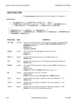


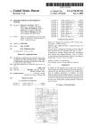


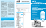
![TwoNav [platform][version]](http://vs1.manualzilla.com/store/data/006156663_1-5deaa8d48af303b2cc7eaad52ecbf272-150x150.png)