1
DPScope II User Manual
Version 1.0
Jan. 8, 2015
Contents
1
Introduction ......................................................................................................................... 1
1.1
General Remarks......................................................................................................... 1
1.2
Software Startup .......................................................................................................... 1
1.3
The Main Screen.......................................................................................................... 3
1.4
First Acquisition............................................................................................................ 4
1.5
Acquisition Modes........................................................................................................ 4
1.5.1
Normal Mode ........................................................................................................ 4
1.5.2
Pretrigger Mode .................................................................................................... 5
1.5.3
Equivalent Time Sampling Mode:.......................................................................... 5
1.5.4
Datalogger (Roll) Mode:........................................................................................ 6
1.6
Probe, Vertical Gain Setup and Trigger Setup: ............................................................ 7
1.7
Undersampling / Aliasing ............................................................................................. 8
2 Description of User Controls ............................................................................................... 9
2.1
Acquisition ................................................................................................................... 9
2.1.1
Run....................................................................................................................... 9
2.1.2
Stop ...................................................................................................................... 9
2.1.3
Clear..................................................................................................................... 9
2.1.4
Continuous / Single Shot..................................................................................... 10
2.1.5
Averaging ........................................................................................................... 10
2.1.6
Log to File........................................................................................................... 10
2.2
Display....................................................................................................................... 11
2.2.1
CH1 / CH2 .......................................................................................................... 11
2.2.2
REF1 / REF2 ...................................................................................................... 11
2.2.3
Lines................................................................................................................... 11
2.2.4
Dots .................................................................................................................... 11
2.2.5
Persist................................................................................................................. 12
2.2.6
Levels ................................................................................................................. 12
2.2.7
Cursors, CH1, CH2............................................................................................. 12
2.2.8
X/Y Mode............................................................................................................ 13
2.2.9
Frequency Spectrum (FFT) / FFT Setup ............................................................. 14
2.3
Vertical....................................................................................................................... 15
2.3.1
Voltage Scale...................................................................................................... 15
2.3.2
Probe Attenuation ............................................................................................... 15
2.3.3
Probe Coupling ................................................................................................... 16
2.4
Horizontal................................................................................................................... 16
2.4.1
Scope Mode / Datalogger (Roll) Mode ................................................................ 17
2.4.2
Sample Rate....................................................................................................... 17
2.4.3
Pretrigger Mode .................................................................................................. 17
2.4.4
Sweep Delay / Trigger Position........................................................................... 18
2.5
Trigger ....................................................................................................................... 18
2.5.1
Auto / CH1 / CH2 ................................................................................................ 18
2.5.2
Rising / Falling / Both .......................................................................................... 19
2.5.3
Noise Reject ....................................................................................................... 19
2.6
Levels ........................................................................................................................ 20
2.6.1
CH1 / CH2 (Channel Offsets).............................................................................. 20
2.6.2
Trg (Trigger Level) .............................................................................................. 21
2.7
File Menu................................................................................................................... 22
2.7.1
Load Setup ......................................................................................................... 22
2.7.2
Save Setup As .................................................................................................... 22
2.7.3
Export Data......................................................................................................... 22
2.7.4
Exit ..................................................................................................................... 23
2.8
Measure Menu........................................................................................................... 23
2.8.1
Measurements .................................................................................................... 23
2.8.2
Spectrum Analysis .............................................................................................. 25
2.8.3
DMM Display ...................................................................................................... 26
2.9
Generator Menu......................................................................................................... 27
2.10 Calibration Menu........................................................................................................ 28
2.10.1 Probe Compensation .......................................................................................... 28
2.10.2 Level Compensation ........................................................................................... 30
2.11 Utilities Menu ............................................................................................................. 31
2.11.1 Comm Setup....................................................................................................... 31
2.12 Help Menu ................................................................................................................. 32
2.12.1 About .................................................................................................................. 32
1 Introduction
The DPScope II is a low-cost, microcontroller based digital oscilloscope intended for hobby and
educational use. It is based on a Microchip dsPIC 16-bit microcontroller. Most of the
oscilloscope hardware is actually integrated in this single chip – analog-to-digital converters,
sample logic, trigger logic and threshold generation, memory, serial data interface. Only the
analog frontend (input amplifier/attenuator, vertical offset generation) and the USB interface
consist of external components.
If you are interested in the detailed hardware design, check out the DPScope II’s webpage
(www.dpscope.com) where you find the full circuit schematic as well as a description of the
hardware functionality and some of the design considerations that went into the development of
this instrument.
If you are new to oscilloscopes, we recommend the following introductory application notes
(created by Tektronix, one of the major oscilloscope manufacturers for the professional, highend market) which will supply all the knowledge necessary to understand this user manual and
get the most from your DPScope II:
The XYZs of Oscilloscopes
The ABCs of Probes
You can download both documents either from the Tektronix website (http://www.tektronix.com)
or from the DPScope II website (http://www.dpscope.com à Downloads).
If after reading through the documentation you still have questions regarding the DPScope II or
want to provide feedback or suggestions for improvement, do not hesitate to contact us at
[email protected]
1.1 General Remarks
The DPScope II is a digital storage oscilloscope (refer to the “XYZs of Oscilloscope” mentioned
in the introduction if you are unsure what that is),
1.2 Software Startup
The software needs the VCP (virtual COM port) driver from FTDI in order to connect to the
scope. Normally this driver is already included with Windows 7 and up or will install
automatically through Windows update. If that is not the case you can also download it directly
from the manufacturer (http://www.ftdichip.com/Drivers/VCP.htm ). After you installed the USB
driver and the DPScope II software, plug in your DPScope II and wait a short time so the
computer has a chance to recognize the scope. The DPScope II’s power LED on the front panel
should blink quickly a few times and then stay solidly on – this is the sign that the scope has
successfully powered up.
1
Then launch the PC software (Start à DPScope II à DPScope II). After a few seconds the
DPScope II program should appear on the screen. If the program cannot connect to the
DPScope II you will get a popup (see below) that you need to confirm in order to continue. The
software will still start after that, but you will not be able to run the acquisition. In this case, close
the software, unplug the oscilloscope, plug it in again (you may want to try a different USB port if
that does not help), and launch the software again.
The DPScope II should always be attached to a USB port directly at the computer, or through a
powered USB hub. Unpowered USB hubs tend to have excessive supply voltage drop which
can potentially create problems and/or lower the scope’s performance.
The scope connects through a so-called “virtual COM port” (VCP), meaning that while the
physical connection is USB, the interface driver makes the connection look like a legacy RS-232
COM port. You can see such ports under “COM and LPT” ports in the Windows device
manager. To find out which virtual COM port the DPScope II uses, go to Utilities à Comm
Setup in the DPScope II program (the software will automatically detect which port the
DPScope II is connected to; in the example below it is COM2, but it can be any port between
COM1 and COM99):
Hint: On some computers the driver seems to have a problems with port numbers larger than
16. If you do see the virtual COM port appear when you plug in the scope (see above) but the
software reports being unable to connect, you can manually modify the assigned port number in
the device manager to 16 or below (make sure not to use a number that is actually used by
another device).
The minimum required screen resolution for the DPScope II software is 1024x768 pixels.
2
1.3 The Main Screen
After startup the screen should look as shown below:
The left side of the display is taken up by the waveform display and a scroll bar to move through
the acquired waveform (the record is longer that what is displayed). On the right side you can
see that the controls are grouped in several functional blocks (we will explain each of them in
more detail later):
·
·
·
·
·
·
Acquisition: Main control of acquisition process
Display: Determines how the acquired data is to be displayed.
Vertical: Controls the input amplification/attenuation for each of the two input channels.
Levels: Sets the voltage offset for each channel, and the trigger threshold level.
Horizontal: Controls the sampling speed, delay, and sampling method.
Trigger: Defines the trigger source.
On the bottom there is a status line that displays the cursor information (right now the cursors
are turned off), which you use to make measurements on the displayed waveforms (e.g. to
determine the signal amplitude or frequency).
On the top of the screen you find the menu containing three several, File (to save the displayed
waveforms in numerical format, and to save and restore the DPScope II’s software settings),
Measure (automated measurements on the waveform and the frequency spectrum), Calibration
3
(gain and offset compensation, and probe compensation), Utilities (connection info), and Help
(displays general info about the software and about the scope’s firmware).
1.4 First Acquisition
After startup the software is set up in a way to maximize you chance to see something useful on
the screen right away: The voltage range is set to maximum, ground level centered on the
screen, continuous mode and trigger in Auto mode (meaning the acquisition will run without
waiting for a trigger event), and so on.
Attach the probes to some signal source, e.g. the toggling output of a microcontroller. Press the
“Run” button. You should see a waveform on the screen. Since the trigger mode is “Auto”, most
likely the waveform will not be stable but rather jump around.
Now play around a bit with some of the controls. Don’t be afraid! You can’t break the scope no
matter what settings you change. The worst that can happen is that you no longer acquire a
waveform and/or see it on the screen. If you get completely stuck, simply close down the
DPScope II program and start it again.
Move the offset sliders and see how the waveforms follow. Now move the trigger level slider so
the trigger level (indicated by a green triangle on the left border of the waveform display) is
somewhere in the middle of the CH1 waveform (the red waveform). Now select “CH1” in the
trigger control menu. That waveform should now be stable (assuming you waveform is periodic).
Try switching between rising and falling edge trigger.
Now change the sample rate in the Horizontal control display and see how the waveform
changes (it’ like zooming in and out on the waveform timing). Move the Sweep Delay slider and
the waveform moving left and right.
In the Display control box, turn the waveforms on and off by clicking on the appropriate
checkbox (you can still trigger on a waveform even when it is not displayed). Change the display
style to points and/or infinite persistence.
Congratulations – you have just measured your first signal with the DPScope II!
1.5 Acquisition Modes
The DPScope II’s acquisition engine has four different modes (again, refer to the “XYZ of
Oscilloscopes” document for further details):
1.5.1 Normal Mode
Acquisition is started by a trigger event (or automatically right after the previous acquisition if the
trigger mode is “Auto”) and samples the signal in real time. This is very similar to how a classic
analog oscilloscope operates. Real-time acquisition means the acquisition is very fast (up to
approx. 30 records per second on a sufficiently fast computer) and you can capture single-shot
4
events. Note that the acquisition rate will decrease for slow sample rates – slower than 50
kSamples/sec or 0.2 ms/div – because it takes some time to simply capture each full record if
only a few samples are taken per second.
Since this mode uses an interrupt generated by the internal hardware comparator the timing is
very tight (i.e. reaction to the trigger event is almost instantaneous), resulting in very low jitter
against the trigger – in practice that means there is very little horizontal (timing) “wiggle” of the
displayed waveform. If the waveform has only little noise, this can sometimes look like the
acquisition has stopped because you only see a steady picture. You can check that it is indeed
running by e.g. increasing the number of averages (combobox in the Acquisition frame) and
ensuring the number bellows counts up.
Normal mode has two limitations: First the maximum sample rate is 2 MSamples/sec (2 million
samples per second), because the controller has to digitize and store the data as fast as it
comes in (up to four Megabytes of data per second since there are two channels!). Second,
since the trigger initiates the capture process, you can only look at things that happen after the
trigger unless you can supply a suitable pre-trigger signal to the second channel to trigger on. If
the waveform is periodic you may be able to use the Sweep Delay feature to trigger on one
edge but look at the following one to get around this limitation.
1.5.2 Pretrigger Mode
In this mode the acquisition runs continuously until the trigger event (e.g. the waveform crossing
the trigger threshold from below, i.e. a rising edge). After the event it keeps sampling for a userdefined time (between zero and one full record length) and then stops, transferring the captured
data to the computer. This means you can now also look at things that happen before the
trigger, which often is the interesting part (e.g. the things that precede a wrong data bit). Since
the acquisition is again happening in real time in this mode you can look at single shot (nonrepetitive) signals, and data acquisition is very fast again. Sweep Delay is not available in this
mode since this feature would not make much sense (after all, if you want to look at things
happening a while after the trigger it is better to use Normal Mode anyway).
The additional versatility of this mode comes with two tradeoffs compared to normal mode. First,
the sample rate is limited to a maximum of 500 kSamples/sec (because in addition to sampling
and storing the signal the scope now must continuously look out for trigger events at the same
time). This is still good enough for the audio range and a bit beyond (up to about 50 kHz).
Second, since the acquisition is completely asynchronous to the signal to be measured, there is
a ±1 sample uncertainty as to how the actual trigger lines up to the sample timing. This results
in increased trigger jitter, i.e. the waveform on the screen will wiggle back and forth by ± one
sample interval (±1/10th of a division).
1.5.3 Equivalent Time Sampling Mode:
This mode works similar to Normal Mode in the sense that the acquisition is initiated by the
trigger event, so again you can only look at things that happen some time after the trigger. But
other than Normal Mode in Equivalent Time Sampling Mode the scope makes no attempt to
sample the signals in a single sweep. Instead it uses its maximum real-time sample rate
(1 MSample/sec or 2 MSample/sec) to capture one or two samples every microsecond, then
5
waits for the next trigger and captures a second record, and so on. For each record it waits for a
slightly longer time after the trigger before it starts sampling; this delay can be controlled in
increments much finer (down to 20 nanoseconds, i.e. 1/50th of a microsecond!) than the
smallest real-time sample interval (0.5 ms). That way – assuming the waveform is repetitive with
respect to the trigger – the sample points of subsequent record will interleave each other with
respect to the actual signal timing. Plotting them together (suitable shifted by the respective
added delay versus the trigger) produces a picture of the signal with finer resolution than
possible with real-time sampling. Once the delay has spanned one full real-time sampling
interval (one microsecond or half a microsecond, respectively), the DPScope II restarts the
acquisition delay from zero delay.
The main advantage is that you can resolve the signal in much finer increments (up to 50
MSamples/sec, or equivalent-time sample intervals of just 20 nanoseconds) than possible with
real-time sampling.
This process of interleaving several acquisitions is implemented in the scope’s firmware (i.e.
running directly on the microcontroller), resulting in very fast and efficient execution, so the
resulting frame rate (number of full waveforms acquired and displayed) is virtually as high as in
Normal Mode (the PC software does not even need to “know” that acquisition for fast
(equivalent) sample rates is different from slower sample rate, in either mode the scope simply
reports when it has acquired a full waveform). Thus as long as the input signal is repetitive you
will hardly notice any visible difference between Normal Mode and Equivalent Time Sampling
Mode.
There are however a few tradeoffs connected with equivalent time sampling. First there is the
necessity that the signals be repetitive with respect to the trigger. Second you always need to
use a trigger to get usable waveforms, otherwise subsequent partial captures will be unrelated
timing-wise, and the composite waveform on the screen will look like random noise rather than
the waveform you expect. Also it’s obvious that you can’t make single-shot acquisitions in this
mode (the software allows single shot mode, but here it means that one full waveform –
consisting of several partial captures – gets acquired and then the acquisition stops). Still, given
the fact that most signals one encounters are repetitive (or can be made repetitive for testing
purposes, e.g. sending a data packet over and over again) means that in practice these
restrictions are far less serious than you might think.
1.5.4 Datalogger (Roll) Mode:
For very slowly varying signals it takes a long time before a full record has been acquired. E.g.
at 1 sec/div timebase each acquisition (80 horizontal divisions) takes 80 seconds, plus the time
it takes before the first trigger event after the end of the previous acquisition happens, so you
may wait over a minute before the screen refreshes just once. In this case it is usually better to
display each sample right when it comes in. This is what the Datalogger Mode (Roll Mode) is
for: The scope acquires the signals continuously and plots the samples on the screen right
away. The waveform scrolls to the left and the new points get added to the right, similar to how
a classic datalogger would draw curves on a moving band of paper from a roll (that’s where the
Roll Mode has its name from).
There is no trigger available in this mode (since we do not want to wait for a trigger event
anyway). But you can log the captured data into a text file on your hard drive, so unlike the other
6
three modes you can capture data sets of arbitrary length, only limited by the free space on your
hard drive. Clearly this mode only makes sense for relatively slowly varying signals, so the
sample rate is limited to 1000 samples per second (timebase 10 msec/div) or slower. Still this is
fast enough to resolve things happening at line frequency (50 Hz or 60 Hz, meaning 20 or ~17
samples per period).
Again sample timing is done by the microcontroller, ensuring very steady and precise timing not
affected by Windows activity (only limitation – once the PCs sample buffer of around 8000
samples runs full, samples will be lost, but even at fastest sample rate this gives a buffer of
several seconds. The scope software will alert you if that happens.).
1.6 Probe, Vertical Gain Setup and Trigger Setup:
When you want to acquire a new (unknown signal), it is best to maximize your chances of
seeing something before fine-tuning your settings. Choose the widest voltage range available (1
V/div) and set the channel offset to the center of the screen. That way your visible range spans
from -10V to +10V (assuming 1:1 probe attenuation) which will capture most signals you
encounter. For larger signal, use a 1:10 probe to widen the range even further (don’t forget to
select the proper probe attenuation in the “Vertical” frame, otherwise the displayed
signal offset will be incorrect!).
Whenever you use a new 1:10 probe, first perform a probe calibration (described in section
“Calibration”). 1:1 probes should not need any calibration because the DPScope II’s input has
been calibrated for them as part of the scope assembly.
It is usually best to set the trigger to “Auto” mode – otherwise you’d have to hunt for a valid
trigger level on the invisible waveform before the scope displays anything. The waveform timing
will not be stable that vay (but will move randomly in time, i.e. waveform “jumping around”
horizontally), but you will be able to see which voltage range the signal spans. Using the
“Persistence” display mode can sometimes be helpful if looking at rare spikes where the signal
amplitude is difficult to judge otherwise.
Once you know the range you can adjust vertical gain and offset to center the signal vertically
and make it fill a good portion (at least a quarter) of the vertical display range.
Note: Due to the way the scope is built, you cannot change the waveform offset when the input
is AC coupled (coupling selection in the Vertical frame). In this case the waveform center is
fixed to the display center.
To set up the trigger, move it to the center of the trigger channel’s signal band (i.e. the green
triangle on the left should be somewhere between maximum and minimum level of the signal –
CH1 or CH2 – you want to trigger on) and turn the trigger on. Switching on the “Levels” display
can be helpful there as well.
To quickly move a slider back to center just press the button labeled “X” (“center”) above the
respective slider.
Now you can fine-tune your setup (e.g. use a different sampling mode, change the trigger
polarity, etc.). When you expect to measure the same signal again later you may want to save
7
the complete setup to a file (File à Save Setup) that can be loaded back later. That way you do
not have to repeat the full setup procedure over and over.
1.7 Undersampling / Aliasing
One very common trap that many beginners (but not only they!) fall into with digital sampling
oscilloscopes is so-called aliasing. This effect can happen whenever the sample rate is too slow
compared to the signal frequency. To pick a simple example, assume you have a 1 kHz sine
wave that you sample with a 1 kSample/sec sample rate. In this case each acquisition will hit
the same point in the signal period (just one period later each time), so the displayed waveform
on the screen will be a flat, horizontal line rather than a sine wave – clearly wrong! If the signal
frequency is a steady 1.1 kHz and the sample rate is 1 kHz each sample will be 1/10th of a
period offset along the waveform, and the resulting displayed waveform will be a very
convincingly-looking 100 Hz sine wave – this can be very misleading! (Incidentally, this is in fact
a variation of the equivalent-time sampling process, called “coherent undersampling”, and is
widely used whenever one can’t get sufficient sample rate to sample incoming high-speed
signals in real time).
The solution is of course to sample the waveform with a sufficiently high sample rate. So if in
doubt, change the sample rate and see if the waveform behaves “normally” (e.g. when doubling
the sample rate the displayed frequency of the signal should not change). And as a general
guideline when working with an unknown signal always start looking at it with maximum sample
rate and only then change it to something slower.
8
2 Description of User Controls
2.1 Acquisition
2.1.1 Run
Starts the acquisition process – data is captured (if trigger event occurs) and displayed on the
screen. If “continuous” is selected the acquisition will repeat until “Stop” is pressed. In case of
“single shot” acquisition the scope acquires and displays only one record and then stops if “No
Avg” (no averaging) is selected; otherwise it will acquire the given number of records to average
over and then stop. This means that if you want to do a true single shot capture you need to set
the averaging to “No Avg”.
In datalogger (roll) mode single shot and averaging is not available; in this case the Run button
simply starts the continuous acquisition.
2.1.2 Stop
Stops the acquisition process.
2.1.3 Clear
Clears the waveform.
9
2.1.4 Continuous / Single Shot
Selects whether the DPScope II shall continuously acquire new waveforms, or only acquire
once and then stop. Continuous acquisition is useful for repetitive waveforms when you want to
see if or how the signal changes over time. Single shot capture is useful e.g. for events that
happen only once (e.g. a sudden pulse), or when you want a steady picture to take
measurements on.
2.1.5 Averaging
Selects how many waveforms to average over (1, 2, 5, 10, 20, 50, or 100). Averaging reduces
random noise on the waveform, resulting in a much cleaner picture that allows you to see small
details that may otherwise be hidden under the noise. For averaging to make sense you need to
have a basically stable, repetitive waveform, so you will need to turn the trigger on (i.e. auto
mode won’t work because the sample timing would be asynchronous to the signal period).
Note that the averaging process used is not a simple arithmetic average over the given number
of samples; instead it uses exponential weighing, i.e. earlier acquisitions have less weight than
the more recent ones. This is the digital equivalent to an analog R-C low-pass filter (but unlike a
filter in your signal path it will not degrade your signal bandwidth or rise time; it will just filter out
fast changes from one capture to the next, but not fast changes along the waveform).
If the signal has changed, and you have selected a large average but don’t want to wait until the
displayed waveform slowly settled to the new shape, simply press “Clear” to restart the
averaging process starting with the most recently acquired waveform.
Averaging is only available in scope mode, not in datalogger mode.
2.1.6 Log to File
This function is only available in datalogger mode. It allows you to write all the captured samples
directly into a file. This way you can record signals of arbitrary time spans and with an arbitrary
number of sample points, no longer restricted to the DPScope II’s 800 points per channel record
length.
10
2.2 Display
2.2.1 CH1 / CH2
Turns the display of scope channel 1 and 2 on or off, respectively. Note that this does not affect
the signal capture itself, meaning you can still trigger on a channel even when it isn’t displayed.
2.2.2 REF1 / REF2
Turns the display of reference waveform 1 and 2 on or off, respectively. To copy the currently
displayed waveform (CH1 or CH2, respectively) into the respective reference waveform you use
the appropriate “à” button.
Reference waveforms are very helpful e.g. to judge small signal changes by comparing the
stored waveform to the displayed waveform.
Another important application is when you want to compare more than two signals; one example
would be an SPI bus consisting of clock, data, and chip select. In this case you can first set up
the DPScope II so CH1 looks at the chip select and CH2 looks at the clock signal, and it triggers
on the falling edge of the chip select signal. Capture both signals with single shot mode, and
save CH2 to REF2. Now connect CH2 to the data line instead, and repeat the capture. You now
have all three signals (clock, data, chip select) on the screen at the same time.
2.2.3 Lines
Checking this option will cause the scope to connect the captured data points with lines. This
makes the actual waveform much easier to see, especially when there are fast changes (which
would make subsequent points fall on places far away on the screen). Use the “Bold” option to
make the lines wider, e.g. to be able to better see them at a distance.
2.2.4 Dots
Checking this option will cause the scope to indicate the actual sample points with small circles.
This can be very useful if you want to check if your sample rate is truly high enough for an
accurate waveform display. Second, use this mode (and turn “Lines” off) when you are in X-Y
11
display mode – if the signals change fast compared to the sample rate, connecting subsequent
sample points with lines can result in a messy, difficult-to-interpret picture on the screen.
2.2.5 Persist
Normally the screen is cleared whenever the scope has a new acquisition is to display.
Checking this option will make the scope keep all waveforms on the screen until you either
press “Stop” and then “Start “ again, or until you press “Clear”. This allows you to see over
which range the waveform is changing; important cases are measurement of peak-to-peak
noise or timing jitter. This is also a great tool to capture rare glitches (sudden waveform
aberrations) that you may miss otherwise because without persist mode they may disappear
from the screen again so quickly that you can’t see them. When persist mode is turned on
however even a single such event with remain easily visible.
Finally a very common application of this mode is to produce so-called data eyes for digital
waveforms. For this purpose choose triggering on “Both” (i.e. rising as well as falling edges) for
the clock waveform, and turning “Lines” off and “Dots” on.
2.2.6 Levels
Turns level markers (and the trigger position marker in pretrigger mode) on and off. While the
levels (CH1 and CH2 offsets, and the trigger threshold) are also indicated with colored triangle
markers on the left edge of the waveform display, sometimes it is helpful to have rulers across
the whole screen. The trigger position in pretrigger mode tells you which portion of the
waveform caused the trigger.
2.2.7 Cursors, CH1, CH2
Turns the measurement cursors on and off, respectively, and selects which channel (CH1 or
CH2) they refer to.
The cursors are the solid horizontal and vertical lines in the waveform display which appear
whenever you check the “Cursors” checkbox. You can move them with the slider bars on
top/bottom and left/right of the waveform display, or alternatively by clicking on them and then
(with mouse button pressed) dragging them to the desired location.
The current level and time positions as well as the difference in their positions are shown in the
status line on the bottom of the scope window:
Because the voltage scales can be different between CH1 and CH2 you need to select which of
these two waveforms the cursors shall refer to. (The time scale is the same for both so this
selection has no bearing on timing measurements, i.e. on the vertical cursors).
12
With the cursors you can perform many different measurements on the displayed waveforms,
for example:
Levels: amplitude, high and low level, average level, overshoot and undershoot
Timing: period, frequency, delay, phase, rise and fall time
Note that the DPScope II also offers a set of fully automated measurements. You can access
them through Measure à Measurements.
2.2.8 X/Y Mode
This checkbox changes between normal (signal versus time, or Y-T) waveform display and X-Y
display mode. In X/Y mode, instead of plotting the CH1 and CH2 waveforms against time, now
CH1 determines the horizontal (X) position and CH2 the vertical (Y) position of each point. A
common application for this is to measure phase shifts, e.g. in order to analyze reactive
elements (inductors, capacitors).
It is usually easiest to first set up the waveforms in normal (Y-T) mode and only then change to
X/Y mode. In addition, usually you will obtain the best picture if you choose “auto” trigger, turn
off “Lines” display and turn on “Dots” and “Persist”.
13
2.2.9 Frequency Spectrum (FFT) / FFT Setup
Checking the “FFT” option will change the display to frequency domain: The oscilloscope
performs a real-time FFT (Fast Fourier Transform) on each captured record and displays the
resulting frequency spectrum. This is a highly useful mode to analyze periodic signals or to find
small periodic components (e.g. periodic noise from the power line) hidden in the main signal –
it is much easier to see an isolated 50 (or 60) Hz component (spectral line) in a frequency plot
than it is to see it among all the random noise riding on the signal. Another common application
is to look at harmonic signal content, e.g. stemming from distortion in an amplifier.
Note that in FFT mode the scope alternates the signal capture between channels, i.e. only
captures one channel at a time. It does that so it can acquire a longer data record (1024 points),
which results in finer frequency resolution. You can still freely choose which channel to trigger
on, i.e. also trigger on a channel when it is not displayed.
Similar to X/Y mode it is usually easiest to first set up the waveforms in normal (time domain)
mode and only then change to FFT mode. Also, in most cases FFT mode works fine in “auto”
trigger mode (as long as the waveform is periodic), and with sample rates low enough so
several signal periods are displayed on the screen. (However, make sure that your sample rate
is at least 3-4 times your signal period, otherwise aliasing will occur, resulting in erroneous
frequency domain pictures – higher frequency components will get “mirrored” into the display
range at the so-called Nyquist frequency, which is half your sample rate).
You can use the cursors to make measurements of frequency and relative power. Note that the
sample rate box changes to frequency units (Hz and kHz).
In addition to cursor measurements the DPScope II software offers fully automated spectrum
measurements which you can access through Measure à Spectrum Analysis: It can
automatically identify the frequency and strength of the fundamental frequency and its
harmonics, and calculate total distortion and noise. These features are described in more detail
in the respective section below.
Selecting the frequency spectrum display also brings up a small panel where you can modify
the settings used for the FFT conversion: Linear (V) vs. logarithmic (dB) scaling, voltage vs.
power, the filter type to use, and finally the averaging method. The filters reduce artifacts
caused by the finite length of the data set. The available types from top to bottom – none,
14
Hamming, Hanning, and Blackman – result in increasingly accurate amplitudes for the price of
increased spectral line width.
At the moment FFT mode is only available in real-time and equivalent time sampling mode, not
in pretrigger mode or datalogger mode.
2.3 Vertical
2.3.1 Voltage Scale
The vertical gain boxes set the input amplifier gain, so you can look at very small (Millivolts) as
well as quite large (several Volts) signals. The scaling is displayed in V/div (Volts per division) or
mV/div (Millivolts per division), so e.g. at 1V/div each vertical unit (interval between two
horizontal dashed grid lines) corresponds to 1 Volt. The settings for CH1 and CH2 are
independent from each other.
The available settings depend on the probe attenuation chosen (see below). Selecting 1:10
probe attenuation will result in all ranges increasing by a factor of 10. Note that this is only a
calculation difference, to be correct you must of course actually have the probe set to the
particular attenuation! (The scope has no way of knowing what you have the probe set to).
2.3.2 Probe Attenuation
The probe attenuation setting (1:1 and 1:10, respectively) does not have any bearing on the
actual input amplifier setup, but rather tells the scope software how it must scale the measured
data on the screen. A 1:10 probe reduces the signal by a factor of 10, which allows you to
measure much larger signals than would be possible with a 1:1 probe. To be correct you must
of course actually have the probe set to the particular attenuation! (The scope has no way of
knowing what you have the probe set to).
Due to the way the DPScope II is designed, the probe used (1:1 or 1:10, respectively)
influences the internal signal offset. Thus it is important to always select the true probe
attenuation, i.e. it is NOT correct to select e.g. “1:1” but use a 1:10 probe – the displayed signal
will have an incorrect offset (e.g. when shorting the probe to ground the display will show a
signal levele offset from zero volts).
15
IMPORTANT WARNING: While the scope can display signals between -200V and +200V with
a 1:10 probe (which reduces these signals to a range between -20V and +20V), you must
exercise extreme caution when working with such large signals (as a rule of thumb, anything
that exceeds 20V is potentially dangerous). If you accidentally touch the source you can
seriously hurt yourself (or even die). To avoid damage to yourself, the DPScope II and/or your
computer, always verify that the probe is truly set to 1:10 mode before contacting the circuit with
the probe. Note that as also stated in the disclaimer on our website, the DPScope II is not
intended for high-voltage applications and as a result we decline any responsibility for damage
or injury resulting from such work with high voltages – you do this at your own risk.
2.3.3 Probe Coupling
In some cases the interesting portion of the signal is only that part that changes. One example
is the measurement of noise (maybe just a few mV) riding on a circuit’s power supply voltage
(several Volts), or some audio signal (where components below ~20 Hz are not audible
anyway). In these cases one wants to suppress the steady (DC) component so one can look at
the AC component with high resolution (a large DC component would otherwise force a rather
coarse vertical gain setting to allow the signal to be displayed). This can be done by adding a
suitable capacitor (“DC blocking capacitor) in series with the signal, which is called “AC
coupling”. The DPScope II has this feature built in, and you can activate it on a per-channel
basis by selecting “AC” in the appropriate combobox.
Note: Due to the way the DPScope II is built you cannot change the waveform offset when the
input is AC coupled. In this case the waveform center is fixed to the display center.
IMPORTANT: Even though the signal will appear centered around zero volts, AC coupling does
NOT increase the maximum voltage level (+/-20V) you can safely apply to the scope inputs!
2.4 Horizontal
16
2.4.1 Record Display Position
While the scope acquires records of 800 sample points per channel, only a range of 200 points
is displayed on the screen. To scroll through the full record, use the slider below the waveform
display (shown in the second picture above). The slider is set up so that a big step corresponds
exactly to a full screen width (i.e. 200 point = ¼ record), and a small step to one horizontal unit
(or, if the “fine” checkbox is checked, to one sample = 1/10th of a horizontal unit). The slider
visualizes the portion of the record currently displayed on the screen. To the right of the slider
the time position of the left edge of the displayed range is shown both in seconds and in
horizontal divisions (zero meaning the start of the acquired record).
2.4.2 Scope Mode / Datalogger (Roll) Mode
In scope mode the DPScope II will always acquire a full data set (800 samples per channel) and
store it in its internal memory before transmitting it to the computer for display. This enables
very fast sample rates (up to 50 MSamples/sec in Equivalent Time Sampling Mode) because
there is no limitation from the transmission speed between scope and computer. The downside
is that the record length is limited to these 800 points, and for very slow sample rates the time
between subsequent transfers becomes larger (because it takes a while to capture 800 points at
a slow rate).
Datalogger (roll) mode on the other hand is limited to relatively slow sample rates (1000
samples/sec maximum, which corresponds to 10 msec/div), but the length of the acquisition is
unlimited, you can have the DPScope II the captured data directly into a text file and thus have
virtually unlimited storage.
2.4.3 Sample Rate
Determines the sample rate, i.e. how many times per second the signals on CH1 and CH2 are
measured. The available range is dependent on the acquisition mode:
Normal Mode, FFT Mode: 1 sec/div to 5 msec/div (10 Sa/sec to 2 MSa/sec)
Equivalent Time Sampling Mode: 2 msec/div to 0.2 msec/div (2 MSa/sec to 20 MSa/sec)
Pretrigger Mode: 1 sec/div to 20 msec/div (10 Sa/sec to 500 kSa/sec)
Datalogger Mode: 10 msec/div to 1 hr/div
2.4.4 Pretrigger Mode
Selects between normal mode (or equivalent time sampling mode) and pretrigger mode. In
Pretrigger mode you can view what happened before the trigger event (up to 80 divisions); the
tradeoff is somewhat higher jitter, and a maximum sample rate of 500 kS/sec. For more details
see the introduction.
17
2.4.5 Sweep Delay / Trigger Position
In normal or equivalent time acquisition mode this slider sets the amount of post-trigger delay,
i.e. the time to wait after the trigger event before the sampling begins. This allows you to look at
the waveform some time after the trigger with high resolution (without that feature you would
have to reduce the sample rate to look at times long after the trigger, because the oscilloscope
has only a limited sample memory (800 points per channel)). For repetitive signals this is
effectively equivalent to a very large sample memory – if you change the slider setting the
waveform will simply seem to move left or right. You can set the sweep delay to any value
between 0 and 200 divisions (be careful at slow timebase settings, since during the sweep delay
the DPScope II will be unresponsive.
In Pretrigger Mode such a sweep delay would not make much sense (after all, you choose this
mode to look at the signal before or around the trigger instant), so it is replaced by a trigger
position selection; this lets you choose how much data shall be acquired after the trigger, or in
other words, where the trigger position shall be within the full record. You can set the trigger
position anywhere from 0 to 100% (0 to 80 divisions) in the record. To display the trigger time
check then “Levels” checkbox in the Display frame.
2.5 Trigger
2.5.1 Auto / CH1 / CH2
The Auto / CH1 / CH2 radio buttons let you select what the DPScope II shall trigger on. A trigger
is basically a condition that determines when the oscilloscope starts the data acquisition. For a
repetitive signal you use this to obtain a steady picture of the signals. For a one-time signal it
allows you to have the scope wait until the event of interest occurs before it starts to capture the
signals.
If set to “Auto” the DPScope II will be free running (constantly collecting data) and not wait for
any special event before capturing data. This is useful when you want to look at an unknown
signal, because you will always see something on the screen (the scope will not wait and not
display anything just because some trigger condition is not fulfilled). Thus this option is available
even in equivalent time mode.
If set to “CH1” or “CH2” the scope will feed the respective channel’s signal into the trigger
circuitry.
18
2.5.2 Rising / Falling / Both
The trigger polarity further specifies the required trigger condition. “Rising” means the signal
must cross the threshold from below and rise above the threshold (i.e. a positive slope) to cause
a trigger. “Falling” means the signal must cross the threshold from above (i.e. a negative slope).
“Both” means the scope will trigger on a rising as well as a falling edge. Of course this will not
produce a steady picture for a repetitive waveform. The most common application for this
feature is to produce data eyes for digital signals (the trigger in this case is the clock signal, the
displayed signal is the data signal). This mode is currently only available in Normal Mode.
2.5.3 Noise Reject
If there is noise on the signal (and there is always some amount) this can cause false triggering.
E.g. if triggering on a rising edge, the signal may actually be falling at a given instant, but a short
little positive noise spike right when the signal has crossed the trigger threshold from above will
look like a rising edge to the comparator and cause a trigger even though it is not a true positive
edge. As a result the oscilloscope will trigger on a falling edge instead of a rising edge.
The “Noise Reject” feature avoids this by requiring that the signal must remain above the
threshold (in the case of a rising edge trigger; below for falling edge) for at least half a division
(i.e. 5 samples). If it fails to do so (e.g. because the edge really was just a short noise spike as
discussed above), the trigger event will get suppressed and the DPScope II will keep waiting for
a trigger.
19
This feature is especially valuable for slowly varying signals. Note however that if your signal
period becomes shorter than about one division, activating the noise reject feature may prevent
the DPScope II from triggering at all. In this case either turn the feature off, or increase the
sample rate so the period becomes a larger fraction of the screen width.
HINT: Similarly, it is recommended to turn off Noise Reject in Equivalent Time Sampling Mode.
Using this mode means that you want to look at a quickly changing waveform anyway, and
since the true sample rate is limited to 1 or 2 MSamples/sec (with a corresponding noise reject
interval of 5 msec or 2.5 msec, respectively) chances are high the noise reject feature more often
than not will prevent signal acquisition in this mode.
2.6 Levels
2.6.1 CH1 / CH2 (Channel Offsets)
Sets the channel offset for input channel 1 and 2, respectively. This lets you control where
ground (zero Volts) is displayed on the vertical axis. First this expands the available voltage
range for a given vertical resolution, e.g. at 1 V/div you could for example cover the range from
0V to +20V, or alternatively from -20V to 0V.
A second use for the offset is to move the two waveforms (CH1 and CH2) apart on the screen
so they are easier to discern, even though in reality they cover similar voltage ranges (e.g. 0V to
5V).
20
The zero position for each channel is indicated on the left side of the waveform display with a
colored marker (red for CH1, blue for CH2). If “Levels” is turned on in the display control frame,
two dashed horizontal lines of same colors are drawn across the display as well at that vertical
position (see picture below).
To quickly move a slider back to center just press the button labeled “X” (“center”) above the
respective slider.
Note: Due to the way the DPScope II is built you cannot change the waveform offset when the
input is AC coupled. In this case the waveform center is fixed to the display center and the
respective offset slider becomes inactive (greyed out).
2.6.2 Trg (Trigger Level)
This slider controls the trigger threshold. If the DPScope II is set up to trigger on one of the
channels (CH1 or CH2), a trigger event occurs whenever the signal crosses this threshold with
the desired polarity (rising or falling edge, respectively, or both rising and falling).
The trigger level threshold for the chosen trigger channel is indicated on the left side of the
waveform display with a green marker. If “Levels” is turned on in the display control frame, a
green dashed horizontal line is drawn across the display as well at that vertical position.
Usually the best approach with an unknown signal is to first display it with trigger in “Auto”
mode. That way – although the waveform on the screen will not be stable – you can at least
judge the voltage range that the signal spans, and set the trigger level marker somewhere within
that range before setting the trigger source to the appropriate channel (see picture below).
To quickly move the trigger slider back to center just press the button labeled “X” (“center”)
above the slider.
21
2.7 File Menu
2.7.1 Load Setup
Recalls a previously saved setup (all settings like acquisition mode, vertical scales, time scale,
trigger setup, etc.) from a file.
2.7.2 Save Setup As
Saves the current setup (i.e. all settings like acquisition mode, vertical scales, time scale, trigger
setup, etc.) to a file.
2.7.3 Export Data
Exports the currently displayed waveforms to a text file. The file contains both scope waveforms
(CH1 and CH2) as well as both reference waveforms (REF1 and REF2). File format is standard
CSV (comma separated values) format, which you can open and process in Microsoft Excel or
any standard text editor (e.g. Notepad).
22
In datalogger (roll) mode it is usually more useful to select “Log to file” instead, because this will
write all the data to the file, while “Export Data” only writes the latest screen interval.
2.7.4 Exit
Closes the DPScope II application. Always close down the application before disconnecting the
scope.
2.8 Measure Menu
2.8.1 Measurements
While it is possible to make measurements on the waveforms using the cursors, the DPScope II
also offers a faster and much more convenient method: Fully automated measurements.
Selecting Utilities à Measurements brings up the Measurement panel. Here you can select on
which channel(s) (CH1 and/or CH2) the software shall take the measurements, and also which
measurements to take. The values get updated after every acquisition. If you have already
acquired the signal and only afterwards bring up the Measurements panel, simply press “Update
Values” to perform the calculation based on the currently displayed waveforms. (Do not change
vertical or horizontal settings like gain or offset between the acquisition and the calculation).
The following measurements are available:
Level: low, high, midlevel, DC mean, amplitude, and AC RMS
Timing: rise time, fall time, period, frequency, duty cycle, positive width, negative width
You can turn the waveform annotations on and off for each channel with the respective
“Annotate” checkbox. If turned on (and the channel is displayed) they will show the low, mid and
high level that the software uses. This can be a valuable tool to troubleshoot your results.
23
Important notes:
·
In order of the timing measurements to work, at least one full signal period needs to be
displayed on the screen.
·
The time measurements employ linear interpolation to improve resolution and accuracy
of the results. This way the resolution of the measurements is much finer than one
sample period.
·
Averaging can significantly improve the accuracy, especially for the level measurements.
·
Measurements slow down the acquisition process somewhat. Turn them off (close the
measurement panel) for maximum screen update rate.
24
Short description of each measurement:
·
·
·
·
·
·
Low: lowest value (minimum) on the screen.
High: highest value on the screen.
Mid: Midpoint between low and high, mid = (low + high) / 2
DC mean: average voltage level, calculated over all points on the screen
Amplitude: difference between high and low, amplitude = high – low
AC RMS: RMS value calculated with the mid level taken as the reference
·
·
·
Rise time: time to rise from 10% to 90% of the swing (low = 0%, high = 100%)
Fall time: time to fall from 90% to 10% of the swing (low = 0%, high = 100%)
Period: time between subsequent rising edges crossings of the 50% point (mid level) (or
falling edges if there aren’t two rising edges on the screen)
Frequency: 1/period
Duty cycle: time spent above 50% during one period, relative to the length of the period.
duty_cycle = pos. width / period
Pos. width: time spent above 50% during one period
Neg. width: time spent below 50% during one period
·
·
·
·
The threshold combobox lets you select which set of levels the measurements shall use for rise
time and fall time measurements – either 10% (start of rising egde / end of falling edge) and
90% (start of falling egde / end of rising edge) of the full swing, or 20% and 80%, respectively.
2.8.2 Spectrum Analysis
25
This panel is only active when the display is set to frequency spectrum (FFT). Here the software
automatically finds the fundamental frequency (the assumption being that what is displayed is a
periodic signal) as well as the first 10 harmonics. It shows both the frequencies (calculated as
center-of-mass of the power spectrum) and the relative amplitudes (corresponding to the area of
each peak), the fundamental being the 100% reference.
Due to the finite resolution of the frequency display and the fact that the signal frequency usually
will not perfectly match a particular frequency point of the calculated spectrum, in many cases
the peaks are not limited to a single point but spread out over at least two frequency “bins” (this
is called “spectral leakage”, with signal “leaking” into adjacent bins). Thus you can select which
width the software shall calculate the total area over (and use for the center-of-mass calculation
of the peak). The default of 7 means it uses 3 points each to the left and to the right of the
peak’s maximum. This method ensures a very precise determination of the actual frequencies.
A setting of 1 is possible but may lead to erroneous results, so a minimum of 3 is
recommended. On the other hand, choosing to large a width will include a considerable amount
of non-harmonic noise in each calculated peak, again affecting the accuracy of the results.
Based on the identified fundamental and harmonic amplitudes the software then also calculates
the total harmonic distortion THD (sum of all harmonic content, i.e. sum of all harmonic peak
areas, divided by the fundamental’s area), noise (total area outside the fundamental and
harmonics, divided by the sum of fundamental and harmonic peak areas), and the sum of both
(THD+N). This is done based on the amplitude (voltage) spectrum – this is the definition
commonly used in the audio area – as well as based on the power (voltage squared) spectrum
– as is commonly done for non-audio applications.
Of course all these calculations will only yield realistic results if the acquired waveform is indeed
periodic.
2.8.3 DMM Display
While the automated measurement panel is convenient, sometimes you may want to observe
only a specific value. This could be e.g. to trim the frequency or the amplitude of an oscillator.
Chances are you do this at some distance from the screen so it is important that the display is
26
large enough to be observable without being right in front of the computer. This is the purpose
for the DMM Display window (DMM stands for Digital Multimeter, because this mode has very
similar functionality to such an instrument). There you can select a single measurement (out of
all the measurements available in the main measurement panel) on one channel, which will then
show up in very large digits.
The update rate lets you select how often the value will get updated (if the acquisition rate is
slow then of course the update rate will be slower than selected, but it will never be faster). This
makes the numbers easier to read since they don’t jump around wildly.
One side note, keep in mind the DPScope (like any other oscilloscope) is an instrument mainly
geared towards display of signal changes over time, not as a voltmeter. Thus the voltage
accuracy or resolution cannot compete with a dedicated DMM - it is limited by the accuracy of
the input divider resistor, the internal voltage reference, and several other factors, so it should
only be used as a rough guidance, or to observe changes in voltage or amplitude rather than
absolute values. As for timing measurements, the accuracy is mostly driven by the clock source,
which has a spec of around +/-0.5%.
2.9 Generator Menu
The DPScope II offers a simple frequency generator. It’s output is available at the CAL pin on
the back side of the instrument. This signal is mainly intended for probe compensation (see
section below) but is also usable for other applications. Note that if you connect this signal to a
circuit you also need to connect the GND pin with the ground (0V) of your circuit. Also make
sure to avoid applying overvoltage (or electrostatic discharges) into the CAL output – while it
does have protection circuitry inside, its protection is not as sturdy as the one for the main
scope inputs!
You bring up the control display through the “Generator” menu. This opens up a window where
you can change the frequency as well as the duty cycle of the signal (dury cycle is the
27
percentage of each period where the output is high). The signal levels are fixed, approximately
0V low and 3.3V high when no load is on the output. The output impedance is roughly 1 kOhm
so if you want to drive a significant load you will need to buffer this signal. (You can however
easily drive a high-impedance CMOS input of a logic gate or a JFET operational amplifier).
To change the frequency or the dury cycle, click on the Up/Down arrows aboce and below the
particular digit. In addition there are a number of buttons on the bottom of the Signal Generator
window that allow you to quickly set a number of common frequencies and duty cycles. The
frequency is adjustable between 250 Hz and 2 MHz (the actual resolution gets coarser with
increasing frequency, so while the display allows changes in single Hz steps this does not
necessarily mean the output frequency will actually change in such small increments).
2.10 Calibration Menu
2.10.1 Probe Compensation
Selecting this menu item puts the DPScope II into probe calibration mode. The software will
automatically set a number of parameters to suitable values (horizontal sale, turning AC
coupling on, setting the trigger level the screen center). Tthe frequency generator – see section
above – is set to produce a 2 kHz square wave with 50% duty cycle).
To perform probe compensation, attach the probe’s signal pin to the CAL output and the probe’s
ground lead to the GND output on the back of the scope. The display will show roughly two
periods of the calibration signal (3.3V amplitude square wave). Depending on the probe you use
(1:1 or 1:10) you may need to adjust the vertical scale and offset to get a decently sized signal
on the screen.
Refer to the calibration panel below as to how the waveform shall look like after calibration. On
the probe there is typically a small screw (either at the probe head itself, or at a small block at
the connector end) that you use to adjust the probe compensation. Since this is a trimmer
capacitor you should use a non-metal (plastic or wood) screwdriver to adjust it – a piece of
metal can detune the setting when it is close, which would make it hard to adjust accurately.
Normally 1:1 probes will not need any compensation – the scope has internal compensation
trimmers that were already set after scope assembly – but if the probes in 1:1 mode do not
produce a clean square wave on the screen (as shown in the window below), the trimmers may
have become detuned during transport and you may want to open the scope and re-do the
calibration (there are only two trimmers in the instrument, one for each channel, so there is no
way to pick a wrong one). Normally though probe compensation is only necessary before using
a new 1:10 probe (and the adjustment is on the trimmer of the probe, not the one in the scope).
Each such probe must be adjusted to match the DPScope II’s (or any other scope’s) input, i.e. it
is usually not sufficient if you performed probe compensation on a different oscilloscope.
28
29
2.10.2 Level Compensation
In this panel you can tell the software to perform a full gain and offset compensation. This is
done to ensure optimum level accuracy (e.g. so that zero input voltage really shows up as
(close to) zero on the screen. It also acts as a relatively comprehensive functional check of the
scope, so it is a useful diagnostic tool if you suspect something is broken.
The set of compensation values is stored in the scope’s EEPROM and is automatically loaded
from there at each program start, meaning the software always uses the appropriate values for
the currently attached DPScope II without user intervention. You can however reload the values
manually, reset the values to default (this only changes the numbers the PC software uses
during the current session, not the numbers stored in the scope unless you manually tell the
software to write them to the scope) etc.
Level compensation is part of the setup and checkout process before each DPScope II is
shipped so the scope is usable right out of the box without you needing to perform this
procedure. It can however be a good idea to execute compensation when using a new set of
1:10 probes because it will optimize offset and gain settings for each particular probe.
To perform this compensation you will need a set of two switchable 1:1/1:10 probes. Normally
the process is fully automated (apart from you attaching the probes and connecting them as
prompted during the compensation execution), but except for serial number and compensation
date you can choose to manually override some or all of the compensation values. For this
press “Unlock Comp Values”. (Note: While you cannot physically damage the scope, no matter
which values you enter, you directly affect the accuracy and validity of the scope
measurements, so do this with care). After finishing your changes, press this button (now
labeled “Lock Comp Values”) again to guard against further modifications. As mentioned above,
the values will be lost when you shut down the software unless you explicitly write them to the
scope (press “Save Values to Scope” to do that). “Sanity Check Values” compares them to the
expected ideal values and highlights in red any that are outside the defined tolerances.
30
To start the compensation process, press the “Start” button of the level compensation panel and
follow the instructions on the screen. At the end, provided all values look reasonable (the
software performs a sanity check against the ideally expected values, using the tolerances
given in the appropriate boxes) the scope will write the new values to the scope. If there are
problems with the results the software highlights (red background) the values that are outside
the tolerance and you will get prompted as to whether you want to overwrite the currently stored
values nevertheless.
2.11 Utilities Menu
2.11.1 Comm Setup
Displays the virtual COM port the DPScope II is connected to. Since detection is automatic, the
“Manual” setup feature is currently always grayed out.
31
2.12 Help Menu
2.12.1 About
Here you can find version and build date of your software, the version of the scope’s firmware,
and finally the serial number of your scope – please always include this information when
submitting bug reports or support requests. The panel also shows the support contact info.
32