Download User Manual

Kionix, Inc.
Wireless Demo Board Kit
User's Manual
September 21, 2007
Table of Contents
I. Zigbee™ - IEEE 802.15.14 wireless standard ............................................... 1
Technical Overview .................................................................................... 1
Product Specifications ....................................................................................... 1
II. Driver Installation & Configuration................................................................ 2
III. Kionix Demo Software................................................................................... 8
1.
Acceleration_Data.............................................................................. 9
2.
Oscilloscope....................................................................................... 9
3.
Data_Logger ....................................................................................... 9
4.
3D Ball............................................................................................... 10
5.
Cursor ............................................................................................... 10
6.
Freefall .............................................................................................. 10
7.
Spaceship ......................................................................................... 10
IV. Sengital Serial MSM Analyzer V4.1 ............................................................ 11
V. Appendices .................................................................................................. 12
Appendix A: Programmer's Manual ............................................................ 12
1. Perl API.................................................................................................. 12
2. Communication .................................................................................... 14
Appendix B: Basic Concepts of Motion...................................................... 15
1. Calculating Velocity and Distance From Acceleration...................... 15
2. Calculating Angle of Tilt From Acceleration ...................................... 16
3. Free-fall Detection ................................................................................ 16
4. Limitations of These Methods ............................................................. 16
Appendix C: Algorithm References ............................................................ 18
1. Converting From Acceleration to Tilt ................................................. 18
2. Controlling a Rolling Ball by Tilting.................................................... 18
3. Detecting Free-fall ................................................................................ 20
4. Jolt Detection........................................................................................ 21
EVALUATION BOARD/KIT IMPORTANT NOTICE
KIONIX provides the enclosed product(s) under the following conditions:
This evaluation board/kit is intended for ENGINEERING DEVELOPMENT, DEMONSTRATION, OR EVALUATION PURPOSES ONLY
and is not considered by KIONIX to be a finished end-product fit for general consumer use. Persons handling the product(s) must
have electronics training and observe good engineering practice standards. As such, the goods being provided are not intended
to be complete in terms of required design-, marketing-, and/or manufacturing-related protective considerations, including
product safety and environmental measures typically found in end products that incorporate such semiconductor components or
circuit boards. This evaluation board/kit does not fall within the scope of the European Union directives regarding
electromagnetic compatibility, restricted substances (RoHS), recycling (WEEE), FCC, CE or UL, and therefore may not meet the
technical requirements of these directives or other related directives.
Kionix warrants that the evaluation board/kit sold will, upon shipment, be free of defects in materials and workmanship under
normal and proper usage. This warranty shall expire 30 days from date of shipment. Kionix will repair or replace, at Kionix’s
discretion, any defective goods upon prompt written notice from the Customer within the warranty period. Such repair or
replacement shall constitute fulfillment of all liabilities of Kionix with respect to warranty and shall constitute Customer’s
exclusive remedy for defective goods.
The user assumes all responsibility and liability for proper and safe handling of the goods. Further, the user indemnifies KIONIX
from all claims arising from the handling or use of the goods. Due to the open construction of the product, it is the user’s
responsibility to take any and all appropriate precautions with regard to electrostatic discharge.
IT IS HEREBY EXPRESSLY AGREED THAT KIONIX MAKES AND CUSTOMER RECEIVES NO OTHER WARRANTY, EXPRESS OR
IMPLIED, THAT ALL WARRANTIES OF MERCHANTABILITY AND FITNESS FOR A PARTICULAR PURPOSE ARE EXPRESSLY
EXCLUDED, AND THAT KIONIX SHALL HAVE NO LIABILITY UNDER ANY CIRCUMSTANCES FOR CONSEQUENTIAL, INCIDENTAL
OR EXEMPLARY DAMAGES ARISING IN ANY WAY FROM THE MISUSE OF ITS PRODUCTS.
KIONIX assumes no liability for applications assistance, customer product design, software performance, or infringement of patents or
services described herein.
No license is granted under any patent right or other intellectual property right of KIONIX covering or relating to any machine,
process, or combination in which such KIONIX products or services might be or are used.
FCC Warning
This evaluation board/kit is intended for ENGINEERING DEVELOPMENT, DEMONSTRATION, OR EVALUATION PURPOSES ONLY
and is not considered by KIONIX to be a finished end-product fit for general consumer use. It generates, uses, and can radiate
radio frequency energy and has not been tested for compliance with the limits of computing devices pursuant to part 15 of FCC
rules, which are designed to provide reasonable protection against radio frequency interference. Operation of this equipment in
other environments may cause interference with radio communications, in which case the user at his own expense will be
required to take whatever measures may be required to correct this interference.
Kionix, Inc. 36 Thornwood Drive Ithaca, NY 14850 www.kionix.com
Page 3
I. Zigbee™ - IEEE 802.15.14 wireless standard
Technical Overview
ZigBee™ is a new global standard for wireless connectivity, focusing on standardizing
and enabling the interoperability of consumer electronic products as well as building
automation and industrial control and monitoring. ZigBee™ is built on the robust radio
(PHY) and medium access control (MAC) communication layers defined by the IEEE
802.15.4 standard. Above this, ZigBee™ defines mesh, star and cluster tree network
topologies with data security features and interoperable application profiles.
The ZigBee™ specification provides a cost-effective, standards-based wireless
networking solution that supports low data rates, low power consumption, security and
reliability. ZigBee™ technology combines interoperable hardware and software to help
make the design process easy and efficient. ZigBee™ technology is suited to a variety
of markets including sensor networks.
Product Specifications
Kionix USB Transceiver
Features:
Specifications:
Freescale MC13191 chipset
16 RF channels
Seven general purpose input/output (GPIO) signals Frequency: 2.4GHz to 2.4835GHz
DSSS Modulation
Indoor Range: 20–40 meters
13 I/O pins for MCU connection
Outdoor Range: 80-100 meters
Four internal timer comparators available to reduce Supports 250 kbps O-QPSK in 5.0 Mhz channels
MCU resource requirements
and full spread-spectrum encode and decode
Programmable frequency clock output for use by
MCU
RX sensitivity of -91 dBm (typical) at 1.0% packet
error rate
Supports MC9S08GT16
Vdd = 3.3V
Supports point-to-point communication
Three power-down modes
0.2 µA Off current
2.3 µA Typical Hibernate current
35 µA Typical Doze current (no CLKO)
Page 1
Features:
Specifications:
Supports point-to-multipoint communication
Physical / Environmental:
Physical size (L * W * H): 52 * 22 * 6mm
Operating temperature: -40 °C to 85 °C
Storage temperature: -40 °C to 85 °C
Humidity: 10% - 90%
Small 52x22x6 mm form factor
Power requirements:
500 µA Idle
30 mA Transmit mode
37 mA Receive mode
•
•
•
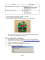
The demo board is powered by a CR2450, 3 volt battery.
The sensor runs at a bandwidth of 50Hz.
The demonstration programs read samples at about 50 samples/second.
Y-
X+
Z+
X-
Y+
•
S1 is a reset button for the module. S2 is a user configurable button (Button 1).
S3 is another user configurable button (Button 2).
II. Driver Installation & Configuration
•
The drivers for the transceiver are available from Future Technology Devices
International, FTDI, as a free download: http://www.ftdichip.com/Drivers/VCP.htm
•
Unzip the FTDI drivers into a new folder
•
Connect the Transceiver to the USB port on the computer
•
Windows will try to configure the device
Page 2
•
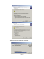
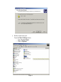
Select the folder that contains the FTDI drivers
Page 3
•
Set the correct com port
From the Start, Settings menu:
o Open Control Panel
o Click on System
Page 4
•
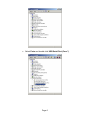
Select Hardware and click Device Manager
Page 5
•
Select Ports and double click USB Serial Port (Com ?)
Page 6
•
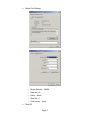
Select Port Settings
o Bit per Second – 38400
o Data bits – 8
o Parity – None
o Stop bits – 1
o Flow control – None
•
Click OK
Page 7
III. Kionix Demo Software
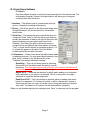
Configure
Run the configure program to set the correct parameters for the demo board. The
configuration program, shown in the figure below, will allow you to configure
communication with the device.
1. Interface – The method used to communicate with the
device. Currently the method is Streaming.
2. Device – The driver specific to the Kionix part being used.
SengitalWireless is the correct device for the wireless
demo board.
3. Serial Port – This selects the port to which the device is
connected. Press “Scan” to limit the list to ports that can
actually be accessed. A label to the right of the button will
appear showing how many ports were found to be
available. Then select the port to which the device is
connected from the address pull-down above, and press
“Test” to check that the device is connected properly. If it
is, a label will appear to the right of the Test button
confirming that the test was a success.
4. Performance – These boxes show the adjustments made
to readings received. You may enter these manually if you
wish, but it is easiest to lay the device flat, press
“Calibrate” and accept the default settings.
Sensitivity – This is a pull down menu for selecting
Figure 1 - configure.pl
the sensitivity of the demo board. Sensitivity is set at
the factory. You must select the correct g level for your board or the demos will
not function properly. The default sensitivity is 2g.
Adjust X/Y/Z – These are the amounts by which each reading on the relevant
axis is adjusted, in g's, before it is returned. This is to account for any slight
variations in center the device might have.
Dead Zone X/Y/Z – This is the minimum absolute value a reading must reach
before it is registered. If it is below this value, it will be read as zero. Having a
dead zone can filter out noise, but at the cost of losing real readings if they are
very small. The default of 0 is perfect for the demonstration programs.
When you are finished adjusting the settings press “Save” to save and exit the program.
Page 8
1.
Acceleration_Data
The Acceleration_Data demo shows the current readings of the
device in the most raw form as is possible. For those interested
in pure data, a device could be attached to a piece of memory to
store a running log of all readings. The data could be retrieved
later for analysis. The actual collection and processing of
accelerometer data does not require very much processor
power, and the sample rate of the device is very high, so an
accelerometer can be added to almost any application while
creating minimal overhead.
2.
Oscilloscope
3.
Data_Logger
Figure 2 - Acceleration_Data
The Virtual Oscilloscope demo graphs data in a simple visual
format to give the viewer a general idea of the pattens
present in the motion of the device. By recognizing these
patterns, such a device could become integral in several
kinds of applications. A free-fall detector could be used to
protect important data by spinning down a hard drive before it
hits the ground. A jolt detector could create a record of
package mishandling during shipping. A vibration detector
could be placed on a piece of machinery to issue an alert if
the pattern of movement changes significantly, indicating the
possible need for maintenance.
Figure 3 - Oscilloscope
The data logger takes a constant stream of readings
from the device and graphs them in real-time to the
screen. Sampling is done by setting the time you
wish to sample, the rate at which you wish to
sample, and pressing “Go”. Note that the sample
rate you specify is the target sample rate. If you
specify a very high number, the program may read
less samples than you expect. If you wish to save
the data you collected, press “Save” to write the
data to a CSV (comma-separated values) file. You
can then use Excel, MatLab, etc. to analyze and
graph the data.
Figure 4 - Date Logger
Page 9
4.
3D Ball
The 3D Ball demo is a simple demonstration of
accelerometer-based controls in video games. By tilting
the device, the user is able to roll the ball around the
board and roll over the red target. Additionally, a strong
bump applied to the z axis of the device will cause the
ball to bounce into the air. A game development team
could use this unique control scheme to add a new level
of playability to games like the classic Marble Madness
by Atari Games, or to create an entirely new game of
their own. Other games which this could be used with
include motorcycle, racing, snowboarding, skateboarding,
and jet fighter games.
Figure 5 - 3D Ball
5.
Cursor
The mouse cursor is a simple demonstration of the idea of a tilt mouse. After opening
the program, the mouse cursor can be moved by tipping the device. To end this
program press CTRL C.
6. Freefall
The Free-fall Detector demo is an example of the free-fall
detection algorithm described in Appendix B. It registers when it
has been in free-fall for half a foot, then reports how far it fell when
it reaches the bottom of its fall. Logging can be temporarily
paused with the “Stop” button, or the log can be saved to a CSV
(comma-separated values) file with the “Save” button. For more
details on the algorithm, see Free-fall Detection in Appendix B.
Figure 6 - Freefall
7.
Spaceship
This Perl program demonstrates how an accelerometer can be
used as a game controller. The tilt action is translated to control
the movements of a virtual spaceship. Avoid the asteroids. If
you crash into an asteroid the “game” will end and need to be
closed and restarted to begin again.
Figure 7 - Spaceship
Page 10
8. Virtual Light Saber
The virtual light saber shows the unique values available
from a tri axis accelerometer. The light saber is activated by
picking up (or moving) the demo board. As you move the
demo board the light saber will mimic your moves. Ten
seconds of inactivity will cause the saber to “turn off”. Moving
the demo board will again activate the light saber.
Figure 8 - Virtual Lightsaber
IV. Sengital Serial MSM Analyzer V4.1
Sengital Limited developed the wireless sensor module using KXPA4 for Kionix Inc.
The Sengital software and manual have been included as another example of
accelerometer analysis software. Use Serial_MSM_Analyzer V4.1 (2.7V).exe to start
the Sengital program. The user manual details the connection procedure.
Page 11
V. Appendices
Appendix A: Programmer's Manual
1. Perl API
The Perl API for the Kionix demo board provides an easy, object-oriented interface for a
Perl programmer to access acceleration data. It is invoked in much the same way as
any other Perl module, and returns an object which can be used to interact with the
sensor.
Usage
Create a new Sensor object from scratch:
use Sensor;
my $Sensor = Sensor->new('Serial', 'TriAxis2g', 'Port' =>
'COM1');
$Sensor->open or warn “Failed to open sensor”;
Create a Sensor object from an existing configuration file:
use Sensor;
my $Sensor = Sensor->newFromConfig('default.ini');
$Sensor->open or warn “Failed to open sensor”;
Sensor Methods
The following methods are universal to all Sensor objects.
Sensor->new($Interface, $Device, %Options)
Create a new object based on the interface driver $Interface and the device driver
$Driver. The %Options hash will be used to override default options if it is
included.
Sensor->newFromConfig($File, %Override)
Create a new object, reading configuration options from $File. The
%Override hash can be used to override options read from the configuration file.
$Sensor->loadConfig($File)
Load configuration options from $File and apply them to $Sensor.
$Sensor->configure($Key, $Value)
Sets a configuration option for the object. Valid options are detailed in “Configuration
Options” below.
$Sensor->open()
Opens the sensor and prepares it for reading. Returns true or false, depending on if
the open was successful.
$Sensor->close()
Closes the sensor. Returns true of false, depending on if the close was successful.
$Sensor->canMeasure()
Page 12
$Sensor->canMeasure($Reading)
$Sensor->canMeasure(@Readings)
When called with no parameters, canMeasure returns a list of all the readings a
sensor can return. When called with one parameter, canMeasure returns a true or
false indicating if that reading can be returned. When called with multiple parameters,
canMeasure returns a true or false value indicating if all of the readings can be
returned.
$Sensor->status()
Returns the status of the device, 1 indicating a ready status and 0 indicating a bad
status. If there is no way to determine the status of the device, this command returns
undef.
$Sensor->$Reading()
Return the desired reading, as indicated by $Reading. $Reading can be any of the
measurements returned by $Sensor->canMeasure(). For an example, see
“Measurements Available From a TriAxis2g Sensor” below.
Measurements Available From a TriAxis2g Sensor
$Sensor->AccX()
$Sensor->AccY()
$Sensor->AccZ()
Returns acceleration on the X, Y, or Z axis. This value is in g's, the acceleration due
to the Earth's gravity. That is, 1g = 9.8m/s². For tilt calculations, 1g = 90º. More
information on using the values returned by an accelerometer can be found in
Appendix B: Basic Concepts of Motion.
$Sensor->Acc()
Unlike the other readings, Acc is a calculated value. It is based on AccX, AccY, and
AccZ, using the Pythagorean Theorem in three dimensions1. It is a measurement of
the magnitude of the acceleration currently being applied to the accelerometer,
without the direction. It is useful for applications such as jolt and free fall detection.
$Sensor->AccAll()
Returns an array of the X, Y, and Z accelerations. Note that because all three of
these are sampled anyway each time any one reading is taken, using this method is
three times faster than calling AccX, AccY, and AccZ in succession.
Configuration Options
The following options can be passed to the configure() method.
Port
This option is accepted by any object using the Serial interface driver. It specifies
which COM port the sensor is plugged into.
AdjustX, AdjustY, AdjustZ
1
Specifically, the calculation used to get overall acceleration is:
2
2
2
a= x +y +z
Page 13
These options are accepted by sensors which can return AccX, AccY, and AccZ
respectively. They are the amount by which the reading is adjusted to account for
slight offsets in the “zero” position of the sensor. These are usually set during a
calibration process, like the one in the configure.pl example script.
DeadZoneX, DeadZoneY, DeadZoneZ
These options are accepted by sensors which can return AccX, AccY, and AccZ
respectively. They specify a minimum absolute value above which each reading must
be. If the reading is within the dead zone for the axis, it is simply returned as zero.
These are usually set to filter out noise when the device is level.
2. Communication
For those who wish to communicate with the device in their own program or
programming language of choice, this section details how communication with the demo
board takes place.
Commands
The following commands can be issued to the demo board once communication has
been established.
Code
Description
Return
X
Get X-axis acceleration.
X (2-byte integer)
Y
Get Y-axis acceleration.
Y (2-byte integer)
Z
Get Z-axis acceleration.
Z (2-byte integer)
A
Return all three axes.
XYZ (three 2-byte integers)
T
Echo a 'T', useful for checking board status.
T (1-byte character 0x54)
Return Values
The value returned for an axis reading is stored as a 2-byte integer in little-endian (least
significant byte first) order. That is, the value can be calculated with the following
equation:
Reading
FirstByte
SecondByte 256
The resulting value represents a number on an arbitrary scale set by the analog-todigital converter taking the reading. To convert this value to millivolts, the following
equation is used:
Millivolts
Reading 1000 1241.2121
Finally, to change the reading in millivolts into the acceleration in g's, subtract the 0g
offset or center (usually Vdd/2, or 1650mv for a 3.3V part). Then, divide by the
sensitivity rating of the part in mv/g. This demo board uses a device with a sensitivity of
660 mv/g, thus:
Acceleration
Millivolts Center 660
The resulting number is the acceleration value returned by the sensor in g's.
Page 14
Appendix B: Basic Concepts of Motion
The concepts discussed in this section are widely available and are a part of any
Physics course, but they have been reproduced here both as a refresher and as a quick
reference useful to anyone working with accelerometer data. There is also a discussion
of the limitations of these methods when used to determine the position or tilt of a
device using a tri-axis accelerometer.
1. Calculating Velocity and Distance From Acceleration
Given an acceleration (a) and a period of time (t), it is possible to calculate the change
in velocity during the relevant time period. If the original velocity is also available, the
velocity at the end of the time period and the change in position over the time period
can be calculated. Lastly, if the original position is available, the position at the end of
the time period can be calculated. This can be done according to the steps below.
Calculating Change in Velocity
Given a, the acceleration applied on the axis.
Given t, the time period for which the acceleration was applied.
v at
Results in ∆v, the change in velocity during the time period.
Calculating Final Velocity
Given ∆v from the previous equation.
Given v0, the velocity at the start of the time period.
v v0
v
Results in v, the velocity at the end of the time period.
Calculating Change in Distance
Given v0 , v, and t from previous equations.
∆d =
(v0 + v )
2
*t
Results in ∆d, the change in distance during the time period.
Calculating Final Distance
Given ∆d from the previous equation.
Given d0, the distance at the start of the time period.
d = d 0 + ∆d
Results in d, the distance at the end of the time period.
Conclusion
At the end of these equations, we have both the final velocity (v) and the final distance
(d). This information can be used to determine the same values in the next time period,
resulting in a continuous flow of acceleration, velocity, and distance data.
Page 15
2. Calculating Angle of Tilt From Acceleration
The acceleration data can also be used to find how far the device is tilted. This can be
done because the Earth is always pulling on the device with 1g of acceleration. If the
device is put on a flat surface and is completely still, all of that acceleration is on the Z
axis. The acceleration on the X and Y axes will be zero. If the object is put on its side,
whichever axis is pointed toward the earth will read 1g. Getting the angle from the
readings on an axis can be done two different ways. The simplest way, although it is not
very exact, is to multiply the acceleration on the axis by 90:
rotation acceleration 90
For a much more exact value, take the inverse sine of the acceleration:
rotation asin acceleration
For more information see Kionix Application Note AN005 on Tilt Sensing
http://www.kionix.com/sensors/application-notes.html
3. Free-fall Detection
A tri-axis accelerometer can be used to detect when an object is in free-fall. The first
step is to calculate the overall magnitude of the acceleration being applied to the object.
This is done with the Pythagorean Theorem:
a = x2 + y2 + z2
If the object is in free-fall, the value will be very close to zero. Depending on the rotation
of the object, however, it may be a somewhat higher number (see “Limitations of These
Methods” below for details). The distance the object fell can be calculated by using
gravity (g = 9.8 m/s²) as acceleration (a) in the equation for calculating distance (d) from
acceleration (a) and time (t):
d=
1 2
at
2
Note that this calculation will produce the wrong number if the object has been thrown
upward or downward. Again, see “Limitations of These Methods” below for more details.
4. Limitations of These Methods
While these equations are effective for many applications, there are several limitations
and “gotchas” that one has to watch for when using the data returned by the
accelerometer.
Noise In Acceleration -> Velocity -> Distance Calculations
All measurements contain a small amount of background noise. Unfortunately, in an
Page 16
acceleration reading, noise can disrupt the apparent velocity of the device. This
difference will become more apparent over time as the “phantom” velocity pushes the
distance measurements farther and farther from reality. This change will be relatively
slow, however, due to the low-noise nature of the device. The difference can also be
made less visible by taking an average of several readings instead of acting on each
reading as it arrives. A dead zone can also be implemented, risking the possible loss of
the actual readings if they are very small.
Differentiating Between Tilt and Motion
While the ability to measure either motion or tilt is very useful, it comes with the
unfortunate disadvantage of not being able to easily differentiate between the two. The
z-axis of this device may make this distinction possible on the x and y axes by watching
the effect of the acceleration in question on the z axis, and the acquired data could be
applied to future demos. Of course, associated equations will also be made available.
Rotation and Center of Mass in Free-fall Detection
Centripetal acceleration, present if the object is rotating, can throw off free-fall detection
by causing the overall acceleration of the object to be significantly higher than zero even
when the object is actually in free-fall. This effect can be reduced by putting the device
in a heavy casing, positioning the accelerometer as close as possible to the device's
center of mass, and allowing a range of values to represent free-fall. 0.0 to 0.5g is
usually a safe range to use.
Free-fall Time When an Object is Thrown
An object is in free-fall as soon as no forces except for gravity are acting on it. That
means that if you throw the device upward, it will be in free-fall even when it is “falling”
upward. Similarly, being thrown downward will shorten the time the object is in free-fall
before it hits the ground. Either of these events will throw off the equation presented in
“Free-fall Detection” above, which assumes that the object was released into free-fall
with a velocity of zero. This limitation is not an issue for applications such as hard drive
protection, as they are only concerned with the fact that the object has been dropped,
but can adversely affect applications in which the distance the object fell is important. In
these cases, it may be better to use an accelerometer with a higher range and
implement impact detection instead of using a low-range accelerometer for detecting
free-fall.
Page 17
Appendix C: Algorithm References
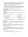
1. Converting From Acceleration to Tilt




2
2 
 Y +Z 
X
roll:
φ = arctan
pitch:
ρ = arctan



2
2 
 X +Z 

Y
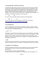
2. Controlling a Rolling Ball by Tilting
Start
Initialize Ball
with position and velocity at zero
Read accelerations X and Y
Add acceleration X to velocity X
Add acceleration Y to velocity Y
Slow velocity X by FRICTION
Slow velocity Y by FRICTION
(The best value for FRICTION depends
on the application)
(The best value for FRICTION depends
on the application)
Add the average of velocity X
to position X
Add the average of velocity Y
to position Y
(The average of velocity X is the average of
the X velocity at the beginning of this time period
and the X velocity at the end of this time period.)
(The average of velocity Y is the average of
the Y velocity at the beginning of this time period
and the Y velocity at the end of this time period.)
Update Screen
Page 18
ball.positionX
ball.positionY
ball.velocityX
ball.velocityY
=
=
=
=
0
0
0
0
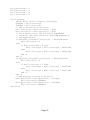
while running
(ACCX, ACCY, ACCZ) = sensor.allreadings
OLDVELX = ball.velocityX
OLDVELY = ball.velocityY
// Add acceleration to velocity
ball.velocityX = ball.velocityX + ACCX
ball.velocityY = ball.velocityY + ACCY
// For a better feel, the following implements
// friction. The best value for FRICTION depends on
// the application.
if absolute_value(ball.velocityX) < FRICTION then
ball.velocityX = 0
else
if ball.velocityX > 0 then
ball.velocityX = ball.velocityX – FRICTION
else
ball.velocityX = ball.velocityX + FRICTION
end if
end if
if absolute_value(ball.velocityY) < FRICTION then
ball.velocityY = 0
else
if ball.velocityY > 0 then
ball.velocityY = ball.velocityY – FRICTION
else
ball.velocityY = ball.velocityY + FRICTION
end if
end if
// Add average velocity to position
ball.positionX = ball.positionX + average(
ball.velocityX, OLDVELX)
ball.positionY = ball.positionY + average(
ball.velocityY, OLDVELY)
end while
Page 19
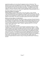
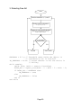
3. Detecting Free-fall
Start
Read accelerations X, Y, and Z
Calculate total acceleration A
A = sqrt{x^2+y^2+z^2}
Compare A to the freefall threshold
Depending on the application, 0.3g to 0.5g is
usually a reliable threshold.
Is A greater
than threshold?
No
Yes
Freefall
Not Freefall
FREEFALL = 0.3 g // Threshold under which the object is
// considered to be in free-fall
IN_FREEFALL = false // Stores whether or not the device is
// falling
while running
(ACCX, ACCY, ACCZ) = sensor.allreadings
TOTAL_ACC = square_root(ACCX ^ 2 + ACCY ^ 2 + ACCZ ^ 2)
if TOTAL_ACC < FREEFALL then
IN_FREEFALL = true
else
IN_FREEFALL = false
end if
end while
Page 20
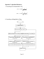
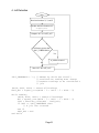
4. Jolt Detection
Start
Read accelerations X, Y, and Z
Calculate total acceleration ACC
A = sqrt{x^2+y^2+z^2}
Compare ACC to LAST_ACC
Difference greater than
JOLT_THRESHOLD?
Yes
A jolt has occurred
No
Store ACC in LAST_ACC
JOLT_THRESHOLD = 1 g //
//
//
//
Amount by which the overall
acceleration reading must change
between readings to be considered a
jolt
(ACCX, ACCY, ACCZ) = sensor.allreadings
LAST_ACC = square_root(ACCX ^ 2 + ACCY ^ 2 + ACCZ ^ 2)
while running
(ACCX, ACCY, ACCZ) = sensor.allreadings
ACC = square_root(ACCX ^ 2 + ACCY ^ 2 + ACCZ ^ 2)
JOLT = absolute_value(ACC – LAST_ACC)
if JOLT >= JOLT_THRESHOLD then
// A jolt has occurred
end if
LAST_ACC = ACC
end while
Page 21