Download User Manual - Decision Support Sciences

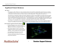
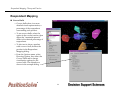
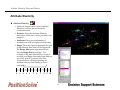
TM
Training Manual
Using Decision Support Sciences’ Dynamic Market
Positioning Tool, PositionSolveTM for Perceptual
Mapping and Marketing Strategy Development
Decision Support Sciences. Better Science. Better Solutions.
Table of Contents
I. Installing PositionSolveTM
V. Product Contouring
System Requirements
Installation Procedure
Theory
Practice
II. Overview of PositionSolveTM
VI. Product Repositioning
What Is Position Analysis
Why Use Multiple Discriminant Analysis?
Introduction To PositionSolveTM Perceptual Maps
Theory
Practice
VII. Appendix
III. Building a Perceptual Map
Dialog Boxes
Using Charts/Graphs
Type of Data Required for PositionSolveTM
Using the SPS Model Wizard
Building the Perceptual Map
Saving the Map
IV. Inspecting Product and Attribute Relationships
Significant Distance Between Products
Closest Competitor Analysis
Respondent Mapping
Attribute Elasticity
Map Options
TM
2
System Requirements
• PositionSolveTM can only be run on a Pentium 200 Processor running Windows 95, 98, NT, or higher. It is
recommended that you have 64 MB RAM, 4 MB of graphics RAM, and at least 30 MB free hard disk space.
Installing PositionSolveTM
• Whether you are installing from a CD or files already on your hard drive, you will run the file
setup.exe.
• During installation, you may choose which directory PositionSolveTM is installed to, and where the
shortcut is accessed from the Start menu.
• PositionSolveTM requires an SPSS SAV file to do position analysis on. In order to go through the
build wizard an create a new perceptual map, it is necessary to have SPSS installed on the same
computer that PositionSolveTM will be used. It is not necessary to have SPSS installed if you are
only working with an existing map.
TM
3
II. Overview of PositionSolveTM
What Is Position Analysis
Why Use Multiple Discriminant Analysis?
Introduction To PositionSolveTM Perceptual Maps
TM
4
Overview of PositionSolveTM
What is Position Analysis?
Position analysis is the process of determining product position in the market relative to competitors as
perceived by consumers. Specifically, the preferences and expectations of a population of respondents for a
set of product attribute variables are analyzed to create a perceptual map of the position of products in the
market.
Position analysis can determine who your closest competitors are, the differentiating attributes of a product
and what specific changes would be most effective in changing a product’s position and capturing market
share.
PositionSolveTM is a discriminant analysis - based perceptual mapping tool*. Perceptual maps are one way to
represent large amounts of information in a way that is interpretable. For example, many variables can be
accurately depicted using a three dimensional map, but only two variables can be viewed at once using a
traditional graph or scatter-plot.
*factor analysis, multi-dimensional scaling, correspondence analysis, and ALSOS techniques are in development.
TM
5
Overview of PositionSolveTM
Why Use Multiple Discriminant Analysis (MDA)?
Multiple Discriminant Analysis (MDA) is the data reduction technique that underlies PositionSolveTM’s perceptual mapping. There
are several reasons MDA was selected as the statistical technique for position analysis. Position analysis is the process of determining
product position in the market relative to competitors as perceived by consumers. Specifically, the preferences and expectations of a
population of respondents for a set of product attribute variables are analyzed to create a perceptual map of the products position in the
market.
Position analysis can determine who your closest competitors are, the differentiating attributes of a product and what specific changes
would be most effective in changing a product’s position and capturing market share.
There are six primary reasons why MDA is used as the data reduction technique in PositionSolveTM.
1)
MDA is familiar to most social scientists as the premier general linear technique used for classification analysis.
2)
MDA (along with factor analysis) is an implementation of the general linear model. Techniques based on the general linear
model can be intuitively and more easily extended to performing dynamic analysis. (Dynamic analyses allow simulation,
movement, and repositioning on a perceptual map.) In the general linear model, the attributes or characteristics of the market
(such as wattage of a microwave oven) serve as predictors of the positioning of the products themselves. Consequently, as you
would expect, when the attributes of a given product are changed, the product “moves,” changing the structure of the space that
underlies the perceptual map.
3)
MDA is the only data-reduction technique designed to produce the maximum separation among products. Since the products
are usually the primary points of interest on the map, MDA’s decision rule to represent the underlying structure of the data with
explicit respect to the products is useful. Conversely, in factor analysis, the focus is solely on the the attributes themselves.
With factor analysis, the products are located as a function of the derived contribution of each attribute to each mapped
dimension, but the resulting interproduct distances are not maximal. In discriminant analysis, however, the dimensions of the
map are based on maximizing variation among products and minimizing variation within products. Consequently, MDA
produces a perceptual map that maximizes interproduct distance.
4)
In the default implementation of PostionSolv, the lengths of the attribute lines, or arrows, represent the direction in which
maximum differentiation among competitors can be achieved. Most product managers are vitally concerned with finding a
unique market niche for their product, maximally differentiating it from the other products in the competitive set. In
PositionSolveTM, by moving a product in the direction of the endpoints of the longest attributes, you are moving it toward
maximal differentiation on those attributes.
TM
6
Overview of PositionSolveTM
Why Multiple Discriminant Analysis (MDA)?
5)
6)
MDA can tell you which attributes are important in the underlying market space, and which you can ignore. Because
discriminant analysis is capable of proceeding stepwise, it automatically discards attributes that do not contribute
significantly to the solution.
Because of its decision rule, when MDA-based perceptual mapping is combined with importance data, the resulting maps
represent both differentiation and importance parsimoniously. Every brand manager recognizes that good strategies are
produced only when you are making changes to a product attribute that is both important and in which there is competitive
differentiation. As mentioned above, MDA-based perceptual maps, especially stepwise ones, include only those attributes
that have strong interproduct differentiation. Thus, if the underlying data are importance-based (such as preference data from
conjoint analysis), the derived perceptual map maximally separates products based on importance data. The strategic power
of this approach is that it combines both importance (via the data source) and difference (via the MDA decision rule) on the
same map. This use of perceptual mapping is also called preference mapping.
TM
7
Overview of PositionSolveTM
Introduction: Basic Interpretation of a Perceptual Map
Feature Description
• There are three dimensions in the graph, and the
axes are represented by a ray that is labeled at
the end with the axis name.
• The X-axis is the primary axis, then the Y-axis,
and finally Z. Using discriminant analysis
methods, as much information and distinction as
possible is shown using the X-axis, and then it
utilizes the Y and Z axes sequentially.
• As a result, if you rotate the graph* so that you
are looking down the Z-axis, there will be little
deviation from the Z plane. But, on the X-axis
there is wide deviation between the attributes
and products.
• The product titles are in bold type, and the
positions are denoted by a large yellow dot. The
product dot represents the centroid, or geometric
center of the attribute scores.
Positioning
• The products are mapped to the screen based on their
relative performance on the selected attributes.
Products that are perceived to be similar in
performance are placed in close proximity on the map.
All else being equal, a product close to the end of an
attribute ray is well-differentiated on that attribute,
whether positively or negatively.
• Attributes: the attribute positions are shown by
lines connected from the origin to the attribute
location. The attribute vector directions and
magnitude are determined by the differentiation
of that attribute. The impact of an attribute on a
product is based on how much consumers base
their reactions to the product on its performance
in a single attribute.
TM
• For example, in this example the Foodware 2000
model is closest to the Low Price and Easy to Use
attributes, so consumer perceive these to be two
important features that characterize the product.
*See the Graphs and Charts section of the appendix for a full
explanation of Graph rotation capabilities.
8
III. Building a Perceptual Map
Type of Data Required for PositionSolveTM
Using the SPSS Model Wizard
Building the Perceptual Map
TM
9
Building a Perceptual Map
Using the SPSS Model Wizard
Step 1
• The dialog box displayed here is the first
step in the ‘Build Model Wizard’.
• There are 5 methods that can be used to
build a new PositionsolveTM map. The
only option available in this wizard at
the current time is MDA.
• All of the steps in the model wizard are
displayed in the ‘Wizard Steps’ box on
the right side of the dialog box. You may
jump to any step at any time by clicking
on the steps in this box.
• All of the selected options may also be
saved in a wizard file from this dialog
box. If you have a saved wizard file, the
options can be loaded by clicking on the
’Load Wizard File’ option.
TM
10
Building a Perceptual Map
Using the SPSS Model Wizard
Step 2 – Select a File Name
• There are two options for creating a map using the
wizard: you may ADD to an existing map or
CREATE a new map.
• If an SDT file has already been created, it will show
up in the left list box. To add to the file, highlight the
file in the box.
• To create a new map, click on the file name text box,
then type a file name for the map file that will be
created.
• The directory that the file will be stored in is listed
above the text box. To change the directory, click on
the desired drive or directory name in the directory
window.
• Make sure that the description at the bottom of the
dialog box is accurate concerning the add/create
mode and the file name and directory.
TM
11
Building a Perceptual Map
Using the SPSS Model Wizard
Step 3 – Select SPSS file
• Click in the box labeled ‘SPSS file’ to select the data file
used for the PositionsolveTM map file.
• The data file must contain attributes, at least one variable
to use as a product, and also segment variables that could
be used to select a segment of the cases based on certain
criteria.
• When the file is selected, the available variables appear in
the left list box. The symbol to the left of each variable
name denotes the variable type. There are four variable
types:
– N=Nominal variables. Any variable that can be asked as a
yes/no question would fit this category
– O=Ordinal variables. Questions where the respondent is asked
to define a rank order for several items are ordinal.
– I=interval scaled variable, which when asked in an interview,
usually requires a text entry answer. This is a continuous
variable.
– R=ratio scaled variable, which is very similar to interval scaled,
but it has a unique rather than an arbitrary zero point. Ratio
scaled variables are also continuous.
• Highlight the variables to be selected in the left list box, then click on
the arrow in the middle to transfer them to the box of selected
variables.
• To see the variable labels instead of the SPSS variable name, click on
the
in the middle of the dialog box.
TM
12
Building a Perceptual Map
Using the SPSS Model Wizard
Step 4 – Select a Product
• From all the variables that are selected to be
included in the map file, PositionsolveTM will
display the variables that could be used as products
because they have 3 or more levels.
• Use the mouse to highlight a variable in the left
box, and the levels for that variable will be
displayed in the level box on the right. Specific
levels can be excluded from the analysis by
deselecting the level with the mouse.
Step 5 – Select Attributes
• Attributes to be included in the map are selected
the same way that the variables were originally
selected. Highlight the variables in the left box,
then click on the arrow in the middle to transfer
them to the box of included variables.
• At least two variables must be included in the map.
• If the ‘Lock these choices as attributes’ option is
selected, the attribute choices may not be changed
after the map is created.
TM
13
Building a Perceptual Map
Using the SPSS Model Wizard
Step 6 – Select Segments
• When the map is created, segments of
the data can be selected for specific
analysis if the segment variables are
selected at this step. You can exclude a
portion of the cases by deselecting
levels in the ‘variable levels’ box.
• Under the variable levels box, the total
number of selected cases is shown, as
well as a poor – excellent rating for that
number of cases.
• Segments do not have to be selected to
create a map. To omit this option,
check the ‘Do not use segments’ box.
TM
14
Building a Perceptual Map
Using the SPSS Model Wizard
Step 7 – Select MDA Algorithms
• Click on the icon to the left of the
method name to select the desired
algorithm(s).
• To use exponents with the selected
analysis methods, click on the exponent
option and select the exponent
restraints.
• ‘Exponent Increments’ refers to the
number of different exponents that are
used. If 10 increments are selected, the
difference between the minimum and
maximum exponent will be divided
into 10 segments, and the exponent at
each of those divisions will be used.
• A summary of the selected algorithms
and exponents is given in the box at the
bottom. The total number of runs will
give you an estimate of the analysis
time to create the map.
TM
15
Building a Perceptual Map
Using the SPSS Model Wizard
Step 8 – Select MDA Criteria
• To determine the specific criteria for
the creating the map, check the box to
use criteria.
• PIN and POUT refer to the required
probability for a variable to be included
or excluded from an equation.
• The top PIN and POUT increment
options are available if the default
option ‘Increment PIN and POUT
separately’ option is selected. If the
increment together option is selected,
the scale at the bottom should be used.
• A summary of the selected algorithms,
exponents, and criteria is given in the
box at the bottom. The total number of
runs will give you an estimate of the
analysis time to create the map.
TM
16
Building a Perceptual Map
Using the SPSS Model Wizard
Step 9 –MDA Data Cleaning
• There are two methods for dealing with missing
data and outliers, using Z scores or setting a
range for the attributes. Based on the option
selected, the specific criteria for that option will
be available.
• If Z scores are being used, select the icons that
represent how the data should be handled.
PositionSolveTM will create several possible maps,
excluding respondents with a z-score of an
absolute value greater than the maximum. The
minimum and maximum set here refer to the zscores to be excluded. The number of Z score
increments can significantly increase the number
of total runs required to create the map.
• If a range is being assigned to each variable,
highlight one or more variables in the list box,
then use the arrows to select the minimum and
maximum acceptable values for the attribute. The
variables that have a range will have a yellow
checkmark by the variable name.
• A summary of the selected algorithms, exponents,
and criteria is given in the box at the bottom. The
total number of runs will give you an estimate of
the analysis time to create the map.
TM
17
Building a Perceptual Map
Using the SPSS Model Wizard
Step 10 –MDA Filters
• First select either 2D or 3D variance.
Currently, only 2D variance is available.
• Check the optional results to be included in
the results. None of these output options are
required for the basic positioning analysis
options once the map is required, but they
may be helpful in the preliminary analysis.
• If a weight variable should be used, check the
weight variable option, then highlight the
variable name in the list box.
• Use the slider to change the attribute
tolerance level. The attribute tolerance is the
amount of dependence or similarity
allowable between attributes. The default
value is 0.001.
• There are three options for filtering the runs,
and any combination of these methods, from
none to all three, can be used to create the
map.
• The product cutoff and the minimum number
of attributes must be greater than 0 for a map
to be created.
TM
18
Building a Perceptual Map
Using the SPSS Model Wizard
Step 11 –Summary
• This screen displays a summary of all the
options that were selected for the current
analysis run. Check through the values to
make sure the options are correct.
• A run title for the current map analysis
must be selected on this screen. Click on
the text to select the title.
• If an option is missing or incomplete, there
will be an error message by the option
name to let you know that it needs to be
modified. You may either click on the
highlighted text to jump to that option, or
select the desired wizard step on the right
side of the dialog box.
• The total number of required runs is listed
at the bottom of the screen.
• When all of the options are complete and
correct, select the ‘finish’ button at the
bottom to begin the analysis.
TM
19
Building a Perceptual Map
Using the SPSS Model Wizard
Run Analysis
• When PositionSolveTM is running the
analysis, SPSS will automatically be
started, and will be running in the
background.
• The Run Information Center dialog
displays the current and best run
detail, and tracks the time required
for all runs.
• The performance tracking section
shows the progress made and
available memory on the computer
being used for analysis.
• The percentage of respondents that
have been correctly classified by
each model are displayed in the
Correct Classification chart.
TM
20
Overview of PositionSolveTM
Introduction: Basic Interpretation of a Perceptual Map
Feature Description
• There are three dimensions in the graph, and the
axes are represented by a ray that is labeled at
the end with the axis name.
• The X-axis is the primary axis, then the Y-axis,
and finally Z. Using discriminant analysis
methods, as much information and distinction as
possible is shown using the X-axis, and then it
utilizes the Y and Z axes sequentially.
• As a result, if you rotate the graph* so that you
are looking down the Z-axis, there will be little
deviation from the Z plane. But, on the X-axis
there is wide deviation between the attributes
and products.
• The product titles are in bold type, and the
positions are denoted by a large colored dot.
The product dot represents the centroid, or
geometric center of the attribute scores.
Positioning
• The products are mapped to the screen based on their
relative performance on the selected attributes.
Products that are perceived to be similar in
performance are placed in close proximity on the map.
All else being equal, a product close to the end of an
attribute ray is well-differentiated on that attribute,
whether positively or negatively.
• Attributes: the attribute positions are shown by
lines connected from the origin to the attribute
location. The attribute vector directions and
magnitude are determined by the differentiation
of that attribute. The impact of an attribute on a
product is based on how much consumers base
their reactions to the product on its performance
in a single attribute.
TM
• For example, in this example the Foodware 2000
model is closest to the Low Price and Easy to Use
attributes, so consumer perceive these to be two
important features that characterize the product.
*See the Graphs and Charts section of the appendix for a full
explanation of Graph rotation capabilities.
21
IV. Inspecting Product and Attribute Relationships
Closest Competitor Analysis
Significant Distance Between Products
Respondent Mapping
Attribute Elasticity
Map Options
Fly Through
TM
22
Closest Competitor Analysis: Theory
Perceptual Mapping is powerful because it is a data reduction technique. It condenses many
dimensions of data down to just a few, enabling an analyst to inspect the closest competitors to his
or her product. Yet, unless 100% of the data are represented in the first two map dimensions, two
products that appear very close may not be; while they may be close on both the horizontal (x) and
vertical (y) axes, they may not be close together at all on the depth (z) axis.
Thus, while the perceptual map doesn’t lie, it may not reveal all of its secrets in the first two
dimensions. The true distance can be calculated using the Euclidean distance formula that takes
into account all of the discriminant functions.) By accounting for all of the dimensions, the closest
competitor analysis identifies the closest competitors to a single product across products.
For example, if there were 30 original products and 30 original attributes, and it took seven
discriminant functions to account for all of the data, the distance measure would be based on all
seven dimensions.
You can calculate the closest competitors to a particular product or calculate closest competitors
from among all products.
TM
23
Closest Competitor Analysis: Practice
Closest Competitor Analysis: Practice
Example 1: Which Products Are Closest Within the Market?
Question:
• What is the “natural positioning ” of the marketplace? Which products are
significantly different on a collection of attributes?
Input Data:
• Importance and performance data collected using conjoint analysis
Steps:
• Open Decision Support Sciences Model
• Open Data File
• Select Base Map
• Select Closest Competitor analysis from command center
• Run Analysis
• Visualize product relationships
• Determine Significant Product Distances
Results:
• Perceptual 3D map of products within the market
• Identification of product distances that are statistically significant
TM
24
Closest Competitor Analysis: Practice
Example 1: Which Products Are Closest Within the Market?
Open Data File
• Select Open from the File menu. The desired data file should be in the
default PositionSolveTM directory. The file will have an .sdt extension.
• Select the file and choose Open.
Open Closest Competitor Analysis
• Select the icon labeled Closest Competitor Analysis on the command
center, or select it from the Inspect menu at the top of the screen.
Analysis Options
• Products: Select on or any number of products from the products box by using the mouse to select or deselect them.
• Cutoff Type: The analysis stops when you exceed the cutoff percentage selected on the Cutoff Percentage slider. If the
“Percentage of Maximal Distance” type is selected (and the cutoff is 50%), the analysis stops once the distance
between the next two products exceeds 50% of the distance from the products that are farthest apart. If the
“Percentage of Product Pairs” option is selected, the top 50% of the competitors are plotted.
• Adjust by Dimension Variance: Since the amount of information contained in each successive dimension drops,
PositionSolveTM ensures that, by default, the scaling of the axes of the map will be proportional to the variance in each
dimension.
• The number of analyses made is determined by the number of products selected and the cutoff percentage. The total
number is displayed in the Comparison Traversal Box or the Distance Histogram.
TM
25
Closest Competitor Analysis: Practice
Example 1: Which Products Are Closest Within the Market?
Visualizing the Analysis
• You can either step through the
visualization of each competitor distance
manually, or let PositionSolveTM
automatically demonstrate each distance
and position the map for a good view of the
product pair.
• To step through the analysis manually,
select the Previous or Next buttons below
the Comparison Traversal slider to see each
product pair.
• A bold yellow line denotes the current
distance being displayed, and other
connections are visible in the secondary
color (default: blue). The model displays
the relationships in order from the closest
competitor to the most distinct, so the first
pair that is shown represents the competitor
that is most similar to that product.
• The current product pair being displayed is
demonstrated along with the distance
variances in the Closest Competitor
Distance Histogram diagram by the yellow
bar.
• If using the animation feature, select the
animate speed by moving the slider, then
select the Animate button.
TM
26
Significant Product Distances
Significant Product Distances
Theory
• The purpose of this analysis is to show which products in the model are statistically separate from one another.
A significant distance cannot be obtained merely by inspecting the perceptual map because statistical separation
is a function of both the distance and the variance around each product. (The greater the variance, or
inconsistency of respondent ratings, the less the distinction.) In fact, even though two products may be far apart
from one another on the map, they may not be significantly different. Conversely, two products close together
may be significantly different from each other. To understand this, we need to remember that each product is the
center of a “cloud” of respondents that rated it. If the cloud around each product is tightly localized, the distance
necessary for the statement that one product is statistically different from another will be smaller.
• This distance is calculated using the Mahalanobis distance between products. The product significant distance
analysis is available only when the indirect methods of the discriminant analysis are used to build the model.
Determine Significant Product Distances
• Under the Inspect menu, select Product
Significant Distance, or choose the Significant
Distance icon from the command center.
• The product distances that are statistically
significant will have a line connecting the two
products. In this example all of the products
are significantly distant from each other.
• Select the Display Attributes option to
visualize the attribute positions in addition to
the product distances.
TM
27
Respondent Mapping: Theory and Practice
Respondent Mapping
Theory
• The respondent analysis, which uses the same formula that plots each product on the map to plot individual
respondents, can greatly enhance your understanding of the perceptual space. Why? Each product plotted on
the map actually represents all respondents who rated that product. Stated mathematically, the product is the
geometric mean of the individual respondent ratings given that product. In essence, each product lies at the
center of a cloud of respondents.
• If this cloud of respondents is tightly localized around the product, market perception of the product is relatively
homogeneous— the respondents hold similar images of that product. Conversely, if the cloud is spread out,
respondents share no strong, consistent product image.
Respondent Mapping
• Under the Inspect menu, select Respondent
Mapping, or select the icon from the command
center.
• Products: From the Respondent Mapping dialog
box, select one or more products to be mapped.
• Overlay: Select an overlay option to display a
circle on the respondent map enclosing a portion
of the respondents. None performs no overlay.
Standard Deviation overlays a circle on the map
one standard deviation away from the product.
Percentile overlays percentiles and Quartile
overlays quartiles.
• If the Percentile option is selected, the Maximum
Percent Enclosed and Sublines Every x Percent
options will be available.
TM
28
Respondent Mapping: Theory and Practice
Respondent Mapping
Convex Hulls
• Convex hulls show, in a more
detailed visual representation, a
percentage of the respondents
surrounding each product.
• To use convex hulls, select the
option in the overlay section, then
adjust the “maximum percent”
slider to the desired percentage of
respondents.
• To elect not to show a product
with a convex hull, deselect the
product in the Respondent
Mapping dialog.
• From the Options menu, select
Drawing Options, then select the
Convex Hulls tab to change
visualization options for the
convex hulls. The defaults are
shown in the example dialog.
TM
29
Attribute Elasticity: Theory and Practice
Attribute Elasticity
Theory
• Attribute elasticity illustrates how far and in what direction a product would move if you changed its rating on
one attribute while keeping all the other attributes constant. Attribute elasticity is instructive for two reasons.
First, it tells you something about that attribute itself. When you plot the attribute elasticity lines or vectors, for a
particular product, the length of the lines differ. Elasticity lines are determined by the discrimination space itself.
If an attribute does not do much to distinguish between products (it has a low F ratio), it contributes little to
determining the discriminant space (at least in the dimensions being plotted). Since it doesn’t define the product
space, it is short. A short line tells you that changing that product’s performance on that attribute won’t move it
much on the map. Conversely, an attribute with a long attribute elasticity line indicates that the products are
relatively different on that attribute. Because the attribute contributes much more to the calculation of the
underlying space, changing its performance has greater potential to move the product on the map.
• Second, and perhaps more important from a practical perspective, attribute elasticity provides information that
you can use when you want to manually reposition a product using a simulation feature. Attribute elasticity will
clearly show you which attributes can change to move a product to a desired position on the map.
Interpreting Attribute Elasticity
• As this diagram demonstrates, a product’s position
on any attribute can be modified positively or
negatively. The attribute continuum goes through
the product locus, but does not originate at the
center. The end of the attribute line without the
arrowhead represents where the product would be
centered if the position of that attribute were
decreased as far as possible. Conversely, the end of
the attribute line with the arrowhead represents
where the product would be centered if the affect of
that attribute were increased.
TM
30
Attribute Elasticity: Theory and Practice
Attribute Elasticity
Attribute Elasticity
• Under the Inspect menu, select Attribute
Elasticity, or select the icon from the
command center.
• Products: From the Attribute Elasticity
dialog box, select one or more products to be
mapped.
• Attributes: Select any combination of
attributes that will be displayed on the map.
• Range: These two options determine the part
of the elasticity lines that will be displayed.
The Range Start percentage must be less
than the Range End percentage. For
example, if the data collected is on a one-toten scale, and Range Start and Range End are
set to 20% and 90%, respectively, then
PositionSolveTM will begin plotting the
attribute elasticity line starting at 2 and
ending 2at 9.
9
0
1
2
3
4
5
6
TM
7
8
9
10
31
Map Options
Map Options
Use the mouse to select Map Options from the command center dialog box.
Dimensions:
The total number of dimensions that contains the map data depends on the multiple
discriminant run. The maximum number on the dimensions slider will automatically be set to
the number of total dimensions for the map. Because of the nature of MDA, most of the data is
contained in the first dimension, and the next highest in the second, etc. The data is usually
mapped to less than five dimensions.
Use the mouse to change the sliders from the default values.
Map System:
Perceptual map elements can be mapped onto the screen in a number of ways. By default,
PositionSolveTM maps the products on the sum of their deviations from the grand mean on each
attribute multiplied by the associated discriminant coefficient for that attribute multiplied by
the associated discriminant coefficient for that attribute. The attributes are displayed as vectors,
or arrows, projecting from the center of the space. By default, these vectors are the discriminant
function coefficients. In the decoupled method, these vectors are the correlations of the
attributes with the discriminant functions. This is called the decoupled method, because the
vectors (which are correlations) are plotted using a different method than the method used to
plot the products. For general use, the default method should be used because it follows a
standard plotting convention.
The disadvantage of using a decoupled method arises when you want to execute the Simulate
menu to see how changing an attribute (such as price) of a specific product moves that product
on the map. With the decoupled method, changing a product on a specific attribute (such as
price) will not necessarily move the product in a direction parallel to the arrow. Consequently,
several coupled methods are available that move the product parallel to the arrow during
simulation exercises.
See the appendix for more details about the Map System Options.
TM
32
Fly Through
Fly Through
When a map has been created, the Fly feature can be used to inspect and maneuver
through the map. The Fly feature can be used with any of the Inspect or Simulate
options.
To open the Fly dialog box, select “Fly” from the Options section of the Command
Center.
Select the “Begin” button to switch the map into free-fly mode. By default, all freeflies will be recorded, but will not be saved unless the user chooses a file name and
location for the fly file.
To effectively maneuver through a map, both the mouse and keyboard should be
used. The mouse changes the perspective angle of the map, and the arrow keys
change the position of the view. For example, imagine you are in an airplane,
viewing the PositionSolveTM map. Moving the mouse changes which way the
plane is facing, and the arrow keys determine whether the plane moves forwards,
backwards, left, or right. So, by using the left arrow key and moving the mouse to
the right to keep the map in view, it is possible to circle completely around the map
at a constant distance from it.
When a fly through is being recorded, the Free Fly controls dialog
and the command center will be hidden. Press the Escape key to
stop the Fly Through and return to the dialog.
When a fly through has been recorded, it can be saved by selecting
the file in the box on the right and clicking on the Save button. If
there are previously recorded fly through files that do not appear in
the box on the right, use the Open button to browse for the files.
To replay an existing fly through, select the file in the box on the
right, and use the playback controls to play the fly through. The
Playback position refers to the position in the fly through sequence.
TM
33
Table of Contents
V. Product Contouring
Theory
Practice
TM
34
Product Contouring: Theory
Product Contouring: Theory
Why is product contouring useful?
• Position analysis seeks to optimize a
product’s position in the market, given a
specified set of constraints. Contouring
determines the boundaries of a product in
any direction, given the constraints set by
the analyst.
• Product Contouring is used with Product
Repositioning to determine realistic
positions and modifications for the
products.
How does PositionSolveTM contour products?
• PositionSolveTM maximizes the ratings on
two or more of the selected attributes at a
time and plots a point where it determines
the combined effect of the attributes would
place the product. The Model then moves
sequentially through all of the selected
attributes, plotting points where it
determines a combination of attribute
modifications would place it. If an
attribute has not been selected in the
constraints, it will not be included in the
contour analysis. A contour is a three
dimensional map that connects all of the
points that are plotted for a specific
product.
TM
• The basic shape of the contour is determined by the
discriminant space, and is also slightly affected by
the product’s position on the perceptual map.
Interpreting Contour Maps
• Products that do not overlap in any way are
perceived as dissimilar and are not competitive
threats to each other given the specified constraints
of attribute movement.
35
Product Contouring: Practice
Product Contouring: Practice
Question:
• What are the constraints on where a product can be repositioned?
Input Data:
• Importance or performance data collected using any number of techniques
Steps:
• Open Data File
• Select Base Map
• Open Product Contouring Dialog
• Select Contouring Options
• Run Analysis
• Visualize product contours
Results:
• Perceptual 3D map of products within the market
• Visualization of repositioning constraints of all products
TM
36
Closest Competitor Analysis: Practice
Example 1: Product Contouring
Open Product Contouring dialog
• Select Simulate, Contouring, or select the icon
from the command center.
Select Contouring Options
• When Product Contouring is activated, this
control panel appears.
• Select one or more products to be included in
the contour analysis using the mouse.
• Select one or more attributes from the
attributes box to be included in the analysis.
• The number of contour attributes selected with
the slider determines the number of attributes
whose magnitude is added together to
determine one endpoint. All of the selected
attributes will, in turn, be included in the
contour map.
• The number of contour lines affects the
number of lines that are used to define the
map, and does not alter the size or shape of the
contours.
• When the attributes are combined to
determine the endpoints of the contours, the
endpoint is displayed along the determined
vector at the percent specified on the Percent
of Maximum slider.
TM
37
Table of Contents
IV.Product Repositioning
Theory
Practice
TM
38
Product Repositioning: Theory
Product Repositioning: Theory
Why use product repositioning?
• Product Repositioning allows products to be
moved to new positions, then develops strategies
for changing attribute performance that will move
the product to that new position. PositionSolveTM
calculates several strategies automatically, so that
the user can simply review the strategies to find
those that are the most actionable.
• Product Contouring is used with Product
Repositioning to determine realistic positions and
modifications for the products.
How does PositionSolveTM reposition products?
• PositionSolveTM uses only the attributes specified
for reposition analysis. Each dimension on the
map is a linear combination of the attributes, so
there are many possible solutions for most
positions on the map. As a result, there are
generally more strategies possible when a product
is closer to its original position. PositionSolveTM
will not change an attribute beyond the range used
to collect the data, so it is possible to position a
product in a place it could not realistically move to.
In this case, no strategies will be displayed for that
product.
• Use Product Contouring to determine reasonable
product positions.
TM
39
Product Repositioning: Practice
Example 2: Product Repositioning
Question:
• What specific steps are required to reposition a product?
Input Data:
• Importance and performance data collected using conjoint analysis
Steps:
• Open Decision Support Sciences Model
• Open Data File
• Select Base Map
• Open Repositioning dialog
• Create and Position New Products
• Set Constraints and Options
• Run Analysis
• View Table and Evaluate Strategies
Results:
• Perceptual 3D map of products positions within the market
• Report of specific necessary attribute changes
TM
40
Product Repositioning: Practice
Example 2: Product Repositioning
Open Data File
• From the File menu, choose Open to select
the data file to open.
Open Product Repositioning dialog
• Select Simulate, Repositioning, or selec the
icon from the control center.
Create and Position New Products
• Check the option to toggle the “Add New
Product Mode.”
• A new product is created by using the mouse
to click on a product dot and dragging it to a
new position (notice the circled products on
the dialog box.) This new product is based
on the product it was created from (the
boxed product), and the new position it is
placed in is analyzed for how attribute levels
must be adjusted from the old levels to reach
the new position.
• If you are not in the Add New Product
Mode, clicking anywhere on the graph and
dragging the mouse will rotate the graph.
TM
41
Product Repositioning: Practice
Product Repositioning
Set Positioning Constraints
• The attributes in the constraints box apply to only one product at a time. Use
the mouse to select or deselect attributes. At least one attribute must be
selected to run the analysis.
• For new products, the constraints can be set specifically, or set the same as
the original product by selecting the Use Parent Constraints option.
• The Search Depth Limit determines the number of attributes that are
combined at once to determine repositioning strategies. Multiple
combinations of attributes are used for each product.
Run Analysis
• Select the Run button, and the repositioning report will be generated.
TM
42
Product Repositioning: Practice
Product Repositioning
View Tables and Evaluate Strategies
• The reports for each new product are accessible by the tabs
at the bottom of the report window. Each new product has
a separate report.
• The visualization of the perceptual map does not change
after the analysis has been run. The map is helpful for
interpreting the results in the repositioning report.
• A position on the map is determined by a linear
combination of the values of several attributes.
PositionSolveTM will not include more than five attributes
in a position strategy. If, in order to reach the new
position, the new value of an attribute would be beyond
the range used to collect the data, the attribute will not be
included in the position strategies.
• The Old and New values are standard deviations from the
mean of the attribute across all products. Therefore, a
value of 0 in these columns would be equal to the mean of
the attribute.
• The Difference column contains the absolute value of the
arithmetic difference between the Old Value and the New
Value.
• The % Diff. column values are a relative difference
between the old and new values of the attributes. Notice
that if the old or new value is close to zero, the percent
difference is significantly greater than if the value is closer
to one.
TM
43
V. Appendix - Reference Manual
A. Dialog Boxes
B. Using Charts/Graphs
TM
44
Reference Manual: dialog boxes
1. File: New
A data file must be opened in
PositionSolveTM to begin the analysis.
PositionSolveTM can create a new file
using an SPSS .sav file.
Select New from the File menu, or the
New File icon to bring up a blank
perceptual map. A wizard will guide
you through the process of importing
the data file from SPSS and setting the
configuration settings of the file.
Browse through available directories
using the
button and selecting
desired directories in the same way that
a file would be opened in standard
Windows applications.
• If the
button is selected,
TM
PositionSolve will exit this dialog box
and cancel any changes that were made.
TM
45
Reference Manual: dialog boxes
1. File: Open
A data file must be opened in
PositionSolveTM to begin the analysis.
Use the Open icon or select Open from
the File menu to get to this dialog box.
Browse through available directories
using the
button and selecting
desired directories in the same way that
a file would be opened in standard
Windows applications.
• If the
button is selected,
TM
PositionSolve will exit this dialog box
and cancel any changes that were made.
TM
46
Reference Manual: dialog boxes
4. Using Charts: Edit Products
Use the mouse to select Edit Products from the command center dialog box.
This dialog box allows you to change the position of products on the map by modifying
specific attribute scores for each product. The product will automatically move on the
map as the attribute score is changed.
Attribute scores can only be changed for products that were contained in the data file.
New products created in PostionSolv have attribute scores based on their parent
products.
To make a change, use the mouse to select one product and one attribute.
Use the mouse to change the vertical slider from the default value.
The product, attribute name, and level are displayed in the box under the attributes.
After an attribute value has been modified, the buttons at the bottom of the dialog box
will be available. Use these reset buttons to return to the default settings for a specific
attribute, product, or all products.
TM
47
Reference Manual: dialog boxes
4. Using Charts: Map Options
Use the mouse to select Map Options from the command center dialog box.
Dimensions:
The total number of dimensions that contains the map data depends on the multiple
discriminant run. The maximum number on the dimensions slider will automatically be set to
the number of total dimensions for the map. Because of the nature of MDA, most of the data is
contained in the first dimension, and the next highest in the second, etc. The data is usually
mapped to less than five dimensions.
Use the mouse to change the sliders from the default values.
Map System:
Perceptual map elements can be mapped onto the screen in a number of ways. By default,
PositionSolveTM maps the products on the sum of their deviations from the grand mean on each
attribute multiplied by the associated discriminant coefficient for that attribute multiplied by
the associated discriminant coefficient for that attribute. The attributes are displayed as vectors,
or arrows, projecting from the center of the space. By default, these vectors are the discriminant
function coefficients. In the decoupled method, these vectors are the correlations of the
attributes with the discriminant functions. This is called the decoupled method, because the
vectors (which are correlations) are plotted using a different method than the method used to
plot the products. For general use, the default method should be used because it follows a
standard plotting convention.
The disadvantage of using a decoupled method arises when you want to execute the Simulate
menu to see how changing an attribute (such as price) of a specific product moves that product
on the map. With the decoupled method, changing a product on a specific attribute (such as
price) will not necessarily move the product in a direction parallel to the arrow. Consequently,
several coupled methods are available that move the product parallel to the arrow during
simulation exercises.
TM
48
Reference Manual: dialog boxes
4. Using Charts: Map Options
Map System:
The advantages and disadvantages of each of the coupled methods are somewhat involved. The
coupled methods are based on different algorithms that combine the standard means of plotting
product (as the sum of attribute deviations multiplied by the discrminant function) with the fact
that each attribute is differentially correlated with each function. In the selection box, the
coupled methods are identified with acronyms based on the algorithm used to locate the
products and attributes on the perceptual map.
Historically, the first coupled method (DW_LW) and the uncoupled method (DC_LC) have both
been widely used. Outside of these two methods, the other coupled methods have not earned as
wide a recognition.
DW_LW The products and attributes obtain their direction (D) and length (L) based on the
discriminant canonical correlation coefficient or weight (W).
DW_LC The products and attributes obtain their direction (D) from the discriminant canonical
correlation coefficient or weight (W) and the length (L) from the correlation of each attribute
with the discriminant function (C).
DW_LB The products and attributes obtain their direction (D) from the discriminant canonical
correlation coefficient or weight (W) and the length (L) from both the correlation of each attribute
with the discriminant function and the discriminant function.
DC_LW The products and attributes obtain their direction (D) from the correlation of each
attribute with the discriminant function (C) and their length (L) from the canonical correlation
coefficient or weight (W).
DC_LC Refers only to the attributes. The attributes obtain their direction (D) from the
correlation of each attribute with the discriminant function (C) and their length (L) from the
correlation of each attribute with the discriminant function (C). The products obtain their
direction (D) and length (L) based on the discriminant canonical correlation coefficient or weight
(W). Because the method for locating the products is different from the attributes, this method is
called decoupled.
TM
49
Reference Manual: dialog boxes
4. Using Charts: Movement
Rotation
There is powerful movement control over all charts created in PositionSolveTM. Move the mouse or use the arrow
keys to change the display of the chart. The labels and text will disappear while the chart is being moved, and the
outline of the attribute vectors and the product positions will give a 3-D image of how how the chart will look.
A chart can be moved to change the angle of perspective on the perceptual map. Moving the mouse vertically or
using the up and down arrows will rotate the chart around a horizontal axis. Likewise, moving the mouse
horizontally or using the left and right arrows will rotate the chart around a vertical axis.
Zoom
Hold down the ‘Ctrl’ key, and move the mouse upward to zoom up, or down to zoom down.
Placement
Hold down the Shift key, and move the mouse to change where the map is centered.
TM
50