Download The Use of Lasers for Pavement Crack Detection

T ec:hnlc:al Report Documentation Page
2. Government Ace• uion No.
1. Report No.
3. Ruiplent'a Catalo; No.
FHWA/TX-~9+1141-1
5. Report Date
4, Tille t1nd SublitJe
The Use of Lasers for Pavement Crack Detection i-;---:::--:--:---=--D_e_c_e_m_b-:=-e-:"r__1_9_8_ 8_--1
6, PerfC?rmlng Orgoni&ollon Code
f--:,...---..,-,.----------------------------t
8.
7. Aurhorf a)
Lynda Donnell Payne, Roger
s.
Performing Orgoni uti on Report No.
1141-1
Walker
10. Work Unit ~o. (TRAIS)
9, Performing Organization Nome and Addrua
The University of Texas at Arlington
Arlington, Texas 76019
Research
Study# 8-18-89-1141
II. Conrroc:t o<. GrGn.t NQ.
~------------------~----------------------------~
12. Sponaorlng Agenc:y Nama and Addrua
Texas State Department of Highways and Public
Transportation, D-10 Research
P.O. Box 5051, Austin, Texas 78763
13. Type of Report ond Period Covered
Interim
14. Sponaoring Agency Code
15. Supplamantarv Natu
Study done in cooperation with US Dept. of Transportation,
Federal Highway Administration
16. Abatract
This research was initiated to investigate the capability of using
lasers for crack detection in pavements. If such a capability could be
developed, it would be used to aid in obtaining and evaluating pavement
distress and cracking information for the State's P.E.S. procedures,
used for maintaining and evaluating pavements.
The research effort has involved three stages. The first two stages
were to determine the crack detection capabilities of the laser probes,
used on the Surface Dynamics Profilometer (DDP).
The SDP is owned by
the State and used for road profile measurements.
After experiments
indicated that these probes could be used for such detection, a system
was developed to further study this capability and to determine how
it could be used to implement an automated high speed crack identification system.
The third stage is the implementation of such a system
so its usefulness for P.E.S. data collection activities can be determined.
This research report describes the first two phases of the
research effort.
18. Oi atribution Stalamant
17, Kay Word a
Surface Dynamics Profilometer (SDP)
Lasers, Pavement Distress Measurements, Pavement Crack Identification and Recording.
19. Security Clouil. (at thia report!
Unclassified
Form OOT F '1700.7
No restrictions. This document is
available to the public through the
National Technical Information
Service, Springfield, Virginia 22161
20, Security Clauif. (olthla poa•l
Unclassified
<8-m
Reproduction of cornpletad pave authorized
21. No, of Pagn
78
22. Price
THE USE OF LASERS FOR
PAVEMENT CRACK DETECTION
by
Lynda Donnell Payne
Roger S. Walker
The University of Texas at Arlington
Research
Report 1141-1
Crack Identification Using Lasers
Research
Project 8-18-88-1141
conducted for
Texas State Department of Highways
and Public Transportation
in cooperation with the
U.S. Department of Transportation
Federal Highway Administration
December 1988
The contents of this report reflect the views of the
authors, who are responsible for the facts and accuracy of the
data presented herein. The contents do not necessarily
reflect the official views or policies of the Federal Highway
Administration. This report does not constitute a standard,
specification, or regulation.
There was no invention or discovery conceived or first
actually reduced in the course of or under this contract,
including any art, method, process, machine, manufacture,
design or composition of matter, or any new and useful
improvement thereof, or any variety of plant which is or may
be patentable under the patent laws of the United States of
America or any foreign country.
ii
PREFACE
This project report presents interim results from Project
8-18-87 1141.
The Project was initiated to determine the
feasibility of using lasers for developing an automated
pavement crack detection and identification system. This
report provides results of the first two phases of the
research effort.
Special recognition is due Mr. Robert Harris of D-18, for
his support in initiating the project and his many
contributions to this research efforts.
Lynda Donnell Payne
Roger S. Walker
December 1988
. .i
ABSTRACT
This research was initiated to investigate the
capability of using lasers for crack detection in pavements.
If such a capability could be developed it would be used to
aid in obtaining and evaluating pavement distress and cracking
information for the State's P.E.S. procedures, used for
maintaining and evaluating pavements.
The research effort has involved three stages. The first
two stages were to determine the crack detection capabilities
of the laser probes, used on the Surface Dynamics Profilometer
(SOP). The SOP is owned by the State and used for road
profile measurements. After experiments indicated that these
probes could be used for such detection, a system was
developed to further study this capability and to determine
how it could be used to implement an automated high speed
crack identification system. The third stage is the
implementation of such a system so it's usefulness for P.E.S.
data collection activities can be determined. This research
report describes the first two phases of the research effort.
KEY WORDS: Surface Dynamics Profilometer (SOP), Lasers,
Pavement Distress Measurements, Pavement Crack
Identification and Recording.
iv
SUMMARY
This project was initiated to determine the feasibility
of using the laser probes on the Surface Dynamics Profilometer
(SOP) owned by the the State Department of Highways and Public
Transportation (SDHPT), for crack detection and
identification. If found feasible a system was then to be
developed for use on the ARAN measurement vehicle, also owned
by the State so it could be used to aid in pavement distress
measurements. The SOP was selected for the initial testing
and evaluation as it had existing on-board laser equipment.
The initial investigations proved that the lasers on the
SOP could be used for crack detection. Based on this result,
the study has proceeded in obtaining the necessary equipment
and developing algorithms and software for implementing an
automated crack measuring system which hopefully could be used
to aid in PES.
This report discusses the first two phases of this
project, determining the feasibility of crack detection using
the laser, and obtaining and testing equipment so such a
system could be implemented. During these first two phases
the capabilities and limitations have been identified.
To date, it appears that a system can be developed with a
limited capability for crack identification and reporting
which could be useful for PES data collection activities. The
third phase of development and implementation of the automated
crack identification system is currently in progress.
v
IMPLEMENTATION STATEMENT
An automated and objective procedure for crack
measurements and recording would provide a significant savings
to the State during P.E.S. data collection procedures. It
could be used in many other areas where statistical
information regarding pavement cracking is desired.
vi
TABLE OF CONTENTS
PREFACE
iii
ABSTRACT
iv
SUMMARY
v
IMPLEMENTATION STATEMENT
vi
LIST OF FIGURES
ix
CHAPTER
I.
II.
III.
INTRODUCTION
1
1.1
Project and Report Scope
1
1. 2
Background
2
1.3
Project Phases
3
1.4
Distress Types
4
1.5
Project Requirements
7
FEASIBILITY
. . . . . .
11
2.1
Sampling and Update Rates .
11
2.2
Resolution, Noise, and Texture
2.3
could Cracks Be Detected? . . • .
12
2.4
The Real-time Issue . . •
13
2.5
Laser Problems and Limitations
17
• • .
18
CRACK IDENTIFICATION HARDWARE
3.1
Optocator . . • . . .
3.2
68000 DAQ Board •
3.3
COMPAQ Portable III • .
18
....
vii
11
24
24
IV.
v.
VI.
TIME AND FREQUENCY ANALYSIS TECHNIQUES .
28
4.1
Time Series .
4.2
Stochastic Process
4.3
Ergodicity and Stationarity .
30
4.4
Statistical Estimates . . .
31
4.5
Power Spectrum Estimation
32
4.6
Linear Parametric Modeling
33
28
...
ANALYSIS OF PAVEMENT CRACKING DATA
. .. . . . . . . ... ... .
29
36
5.1
Introduction
5.2
Variance Method for Real-Time
Crack Counting
. . . .
36
5.3
Spectral Analysis Results . . .
37
5.4
Running Mean/Slope Threshold Method
38
5.5
Autocorrelation Difference Method .
41
5.6
AR Process Modeling Results
46
CONCLUSIONS AND FURTHER RESEARCH .
36
49
APPENDIX
A.
DAQ BOARD SCHEMATICS • • . .
52
B.
RUNNING MEAN/SLOPE THRESHOLD LISTING .
59
65
REFERENCES . . . . . . • •
viii
LIST OF FIGURES
. ..
1.1
Rutting .
1. 2
Patching
1.3
Failure . .
1.4
Alligator cracking
1.5
Block cracking
8
1.6
Transverse cracking .
8
1.7
Longitudinal cracking
9
2.1
Laser probe and laser calibration board .
14
2.2
Laser orientations
15
2.3
Calibration board results •
16
3.1
Laser probe and probe processing unit .
19
3.2
Pulsed, modulated infrared light from
GaAs lasers . . . . . •
. . . .
21
3.3
Triangulation principle . .
22
3.4
Laser measurement range .
23
3.5
CPU sub-rack with power supply and
receiver-averaging boards • . • .
25
3.6
Data acquisition (DAQ) boards .
27
3.7
Crack system in the profilometer
27
5.1
Power spectral density plots of different
cracking types . • . . . . . . • . . • .
39
Power spectral density plots of different
cracking severity . • . . • . . . . . . .
40
5.2
......... ..
....
. .. .
ix
5
5
6
6
5.3
5.4
Running mean/slope threshold technique applied
to moderate alligator cracking data . . . . . . .
42
Running meanjslope threshold technique applied
to severe alligator cracking data . . . .
43
. . ....... . . . . . . . . .
5.5
Raw data
5.6
Filtered data with r(O)-r(4) value plotted
every 16 data points . . .
. . . .
47
Actual r(O) and r(4) values for the data
in Figure 5.6 . . . • • . .
. ..
48
5.7
45
CHAPTER I
INTRODUCTION
1.1
Project and Report Scope
This project was initiated to determine the feasibility
of using the laser probes on the Surface Dynamics Profilometer
(SDP) owned by the the State Department of Highways and Public
Transportation (SDHPT), for crack detection and
identification. If found feasible a system was then to be
developed for use on the ARAN measurement vehicle, also owned
by the state. The SDP was selected for the initial testing
and evaluation as it had existing on-board laser equipment.
As will be discussed initial evaluations proved that the
lasers on the SDP could be used for crack detection. Based on
this result, the study has proceeded in obtaining the
necessary equipment and developing algorithms and software for
implementing an automated crack measuring system for PES.
This report discusses the first two phases of this
project, determining the feasibility of crack detection using
the laser, and obtaining and testing equipment so such a
system could be implemented.
The third phase of development and implementation of the
automated crack identification system is currently in progress
and will be reported on in a later report.
This introductory chapter will first provide a background
and general understanding of the crack detection and
identification problem. Further, it explains some necessary
terms and describes the project requirements. Chapter two,
then addresses the feasibility issue. It describes the work
done to determine if pavement cracking could be detected with
the lasers. The third chapter describes the hardware designed
and built for initial evaluation of a crack detection system.
Chapter four defines and explains the statistical and signal
processing theory used in the crack identification algorithms.
Chapter five describes the different crack identification
algorithms employed. This chapter also describes results of
the data analysis on the test sections used in the study.
1
2
Chapter six describes additional research, much of which is
being conducted in the third phase.
1.2
Background
The evaluation of pavement surface conditions of the
nation's highways is of major interest to transportation
engineers. The State has been using such information in
conjunction with other data in an established procedure for
determining the condition of the State's highway system. This
information is essential in determining which roads should be
worked on, and how much money is needed to complete the work.
The State currently evaluates pavement surface conditions
by considering both road roughness and pavement distress. A
measure of road roughness is readily obtained with existing
instruments.
Pavement distress information is more difficult
to obtain as it requires visual evaluation. Currently, SDHPT
personnel attend the annual Pavement Evaluation System (PES)
Rater Training School and then disperse to their respective
districts throughout the state to rate pavement surfaces by
"walking" the roads. Obviously, this process is very tedious
and time-consuming. Also, since so many people are involved
in the evaluation, the ratings are often not repeatable. An
automated measurement system is needed to simplify the process
and to obtain more consistent measurements.
This research represents the first attempt by the SDHPT
to automate the process. The research was made possible when
laser probes were purchased for use on the Surface Dynamics
Profilometer (SOP). The SOP is used by the Department to
obtain road profile measurements. Two lasers, one in each
wheel path, are used to measure distances from the bottom of
a survey vehicle to the road surface. These distance
measurements, along with vertical acceleration measurements
from two accelerometers, are used to obtain the road profile
by removing the effects of the vehicle suspension system
[1,2,3].
The laser system discussed in this study is built by
Selective Electronic Co. (Selcom) of Sweden. The device is
called an optocator. The system's basic components are the
laser probes and probe processing units, which are mounted
under the van, and the CPU sub-rack containing the power
supply and receiver-averaging boards, which are installed
inside the van.
The optocator measures distances to a surface using laser
probes. Each probe emits a small infrared light beam that
strikes the surface to be measured. The reflected light is
focused onto a position-sensitive detector in the laser probe
allowing accurate distance measurements [5]. Further
explanation of the optocator and measuring principle wi!l be
provided in Chapter III.
Since the lasers were available, highway department
engineers wanted to know if these lasers could help identify
pavement cracking.
The intent of this study was first to
determine the feasibility of using the existing lasers of the
SDP to identify pavement cracking.
Then, if feasible, the
work would be extended to design and implement a system which
would identify the specified cracking patterns.
Few
operational systems for crack identification using aser probes
have been reported in the literature.
Most studies for such
systems have used video data [6,7].
The research herein does
not u~e an elaborate video camera system, only existing
lasers.
1.3
Project Phases
As noted above, this study consisted of three phases and
this report is concerned with the first two phases.
First,
the feasibility of using the existing laser probes on the SDP
had to be investigated.
This involved determining whether or
not the resolution of the laser probes was sufficient to
detect cracking patterns.
Also, the measurement update ra~e
had to be considered to determine if the laser could supply
the necessary sampling rate for crack identification at
highway speeds.
Another item of interest was the real-time
issue.
That is, how much, if any, of the processing and
analysis could be performed in real-time with the van moving
at highway speeds? If real-time computation was not feasible,
what procedures could be developed to collect data for later
processing?
Phase two was to begin once it was determined that crack3
could be detected using the laser probes.
This phase would
involve designing, testing and implementing both the hardware
and software for a system which could be used for crack
detection and identification.
Although it has been stated that phase one was first
investigated followed by phase two, this was not exactly the
case.
Obviously, some of the issues in phase one could only
be addressed if there existed hardware and software to obtain
the cracking data.
In actuality, the phases overlapped and
some of the hardware and software developed will be changed
later based on results obtained.
By the same argument the
success of such systems can only be determined by actual
implementation.
4
1.4
Distress Types
This research is only concerned with distress types in
asphalt surfaced pavements since this type of road surface
repres~nts the largest percentage
of the highway system in
Texas.
The distress types which are currently recorded by PES
raters on asphalt pavements are rutting, patching, failures,
alligator cracking, block cracking, transverse cracking, and
longitudinal cracking [8). Each type will be described here
for completeness; however, not all types are considered in
this research.
A rut is a surface depression in the wheel paths.
Rutting stems from a permanent deformation in any of the
pavement layers or subgrade. It is usually caused by
consolidation or lateral movement of the materials due to
traffic loads. Refer to Figure 1.1.
Patches, shown in Figure 1.2, are repairs made to
pavement distress. The presence of patching indicates prior
maintenance activity, and is thus used as a general measure of
maintenance cost.
A failure is a localized section of pavement where the
surface has been severely eroded, badly cracked, or depressed.
Failures are important because they identify specific
structural deficiencies which may pose safety hazards. see
Figure 1.3.
Alligator cracking is a series of interconnecting cracks
caused by fatigue failure of the asphalt surface under
repeated traffic loading. The cracking initiates at the
bottom of the asphalt surface where tensile stress and strain
is highest under a wheel load. The cracks propagate to the
surface initially as one or more longitudinal parallel cracks.
After repeated traffic loading the cracks connect, forming
polygon-shaped, sharp-angled pieces that develop a pattern
resembling chicken wire or the skin of an alligator. The
pieces are usually less than 1 foot on the longest side.
Alligator cracking occurs only in areas that are subjected to
repeated traffic loading. Refer to Figure 1.4.
Block cracking divides the asphalt surface into
approximately rectangular pieces. The blocks range in size
from approximately 1 foot square to 100 feet square. See
Figure 1.5. Cracking into larger blocks are generally rated
as longitudinal and transverse cracking. Block cracking is
caused mainly by shrinkage of the asphalt concrete and daily
temperature cycling. It is not load associated, although load
can increase the severity of individual cracks. This type of
5
Figure 1.1
Figure 1.2
Rutting
Patching
6
Figure 1.3
Figure 1. 4
Failure
Alligator cracking
7
distress differs from alligator cracking in that alligator
cracks form smaller, many-sided pieces with sharp angles.
Also unlike block cracks, alligator cracks are caused by
repeated traffic loadings.
Transverse cracking, seen in Figure 1.6, consists of
cracks or breaks which travel at right angles to the pavement
centerline. Transverse cracks are usually caused by
differential movement beneath the pavement surface. They may
also be caused by surface shrinkage due to extreme temperature
variations. Although transverse cracks may occur at any
spacing, they will be only considered such for this research
if they occur at distances greater than 10 feet apart. More
closely spaced cracks are counted as either alligator or
block. PES data and SDHPT experience suggests that this
assumption will cause only a minor error in statewide PES
sections.
LongitL:inal cracks are parallel to the pavement's
centerline cr laydown direction. They may be caused by a
poorly constructed paving lane joint, shrinkage of the surface
due to low temperatures or hardening of the asphalt, or a
problem with the subgrade. Refer to Figure 1.7 ( Note the
figure also has block cracking).
ThJsJ:esearch effort considered only three of the seven
.EJ_stt:ess. types described above. Specifically, alligator, - block, and transverse cracking were to be considered. Some of
the other distress types, particularly failures and
longitu~inal cracking, could cause the cracking pattern to be
misclassified due to the nature of the sensors used and the
method of observation. This should become clear from later
discussions.
1.5
Project Requirements
As previously described, this study involved using the
existing lasers to identify cracking patterns . One laser was
to be mounted in each wheel path, and one in the middle.
Obviously, little, or no information across the lane could be
recorded to help in the identification. The laser data was to
be recorded and analyzed in real-time at highway speeds if
possible.
The type, severity and percent area of cracking was to be
determined from the laser data obtained. Type refers to one
of the three types previously mentioned (alligator, block, or
transverse). Severity is determined by the width of the
crack. Slight cracks are less than 1/8 inch, moderate are 1/8
to 1/4 inch and severe are greater than 1/4 inch wide. Also,
the percent of the section with each type of crack was to be
noted. In the case of transverse cracks, a count of the
. --
8
',
'-:. +v.,;.f'.J.'_...,:_
;1t'~:
r
::,
~,~'-- ..
i
r
Figure 1.5
Figure 1.6
Block cracking
Transverse cracking
9
Figure 1.7
Longitudinal Cracking
•.
10
number of cracks detected in a section length was to be
reported.
Finally, if the complete data analysis and reporting
could not be performed in real-time, then at least a
reasonable (1 mile) length of data should be recorded in realtime. It could later be downloaded and further analysis and
reporting performed.
10
CHAPTER II
FEASIBILITY
2.1
Sampling and Update Rates
The first question to be addressed in phase one was
whether or not the lasers could provide measurements at a
sufficiently fast rate. That is, did the laser update rate
meet or exceed the necessary sampling rate? Since the
smallest cracks to be detected were in the 1/8 inch wide
range, it was reasonable that a 1/16 inch sampling rate would
be required.
The update rate of the Selcom laser system is fixed with
jumpers on the receiver-averaging board in the CPU sub-rack.
This is discussed in Chapter III. However, the maximum update
rate (no averaging) is 32,000 samples per second [4,5].
The necessary sampling rate for 1/16 inch sampling varies
from 2816 samples per second at 10 miles per hour to 14080
samples per second at 50 miles per hour. A comparison of the
update rate to the maximum required sampling rate shows that
the Selcom lasers are able to supply measurements at the
necessary speed. Also, since the update rate is more than
twice the required sampling rate it is suggested that the
receiver-averaging boards be jumpered for two point averaging.
This will provide a 16K update rate, still exceeding the
sampling rate required, and at the same time reducing the
noise in the measurements.
2.2
Resolution, Noise, and Texture
The laser measurement range, as explained in Chapter III,
is 10.04 inches. The analog signal from the laser probes
varies from 0 to 10 volts. A 12-bit A/D converter in the
probe processing unit (PPU) converts the analog signal into a
12-bit digital representation, providing a 2.44 mv or .00245
inch resolution.
Noise is a major consideration in determining measurement
accuracy and the ability to detect cracking. That is, how
much variability in measurement readings would be expected if
the laser was reflecting off a surface at a constant distance?
11
12
To determine this the range and variance of two data sets was
considered. In the first, the lasers were bench mounted in
the lab and data was collected with the laser beam reflecting
off a flat stationary object. Results from this procedure
showed a range of + 28.9 to - 32.1 mv _from the mean with a
standard deviation of 7.9 mv.
A second set of data was collected in the profilometer
with the motor running and the van at rest. Here the range
was+ 36.0 to- 37.2 mv from the mean and a standard deviation
of 16.8 mv was observed. These observations were needed to
provide insight into reasonable threshold values used in
several of the crack detection algorithms.
The texture
variability. In
surfaces of very
reasonable crack
study.
2.3
of a road surface is another item which adds
fact, it should be understood that road
course texture probably do not allow
detection by the methods described in this
Could Cracks Be Detected?
Phase one of this project involved determining whether or
not the Selcom lasers on the profilometer could detect cracks
in a road surface. Two approaches were taken to answer this
question. First, short sections of pavement with the desired
cracking were located. The sections were marked as to start,
end, and the desired path for the driver to take. Laser data
was then obtained from the sections with the driver being very
careful to follow the marked path. This data was plotted and
compared with slides taken of the marked section. Results of
this comparison were very encouraging. Most of the moderate
and severe cracks seen in the slides could easily be
recognized in the plots.
The first procedure.of driving over a marked section gave
a good idea but it was never known exactly where the laser
beam fell. That is, a crack perpendicular to the centerline
may be 1/4 inch wide at one point while 1/2 inch over it might
be 1/16 of an inch wide. For this reason, that procedure did
not give much insight into how well the lasers would be able
to provide severity information. Therefore, a surface with
cracks of known width and depth was needed for testing. To
provide this known surface the laser calibration board was
built.
The laser calibration board, though simple in concept and
construction, provided valuable information. This board was
simply a circular piece of black plywood suspended from a
variable speed motor. Cracks of different widths and depths
were cut into the board surface. The board was cut with a
desired circumference so it could easily simulate a road
surface passing under the laser probes at speeds from 1 to 30
miles per hour by varying the rotational speed.
Three different sets of cracks were cut into the board.
Cracks within each set were the same depth.
That is, one set
of cracks was 1/8 inch deep, one set was 1/4 inch, and the
third set was 3/8 inch in depth.
Five cracks of varying width
were cut in each set.
They were 1 inch, 1/2 inch, 1/4 inch,
1/8 inch, and 1/16 inch.
Figure 2.1 shows the bench mounted
laser probe, PPU, and the laser calibration board.
One important observation which came to light while
working with the calibration board was that orientation
significantly affected measurements.
As will be discussed in
Chapter III, the laser beam which strikes the measured surface
is longer in one direction than the other.
It was found that
the ability to detect slight cracking was significantly
improved by having the laser beam fall across a crack
perpendicular to the centerline instead of into the crack.
That is, orientation 2 in Figure 2.2 gave much better results.
Also, orientation 1 gave invalid data readings on the back
side of pratically every crack.
Invalid data is typically
caused by an insufficient amount of laser light falling on the
detector.
Orientation 2 showed no invalid data.
This
observation can be explained by the fact that the entire beam
fell into the crack in orientation 1 and the path of the
reflected light back to the detector was obstructed by the
crack wall as the beam neared the back side of the crack.
Figure 2.3 provides a plot of laser measurements obtained
from the calibration board at 15 miles per hour using
orientation 2.
It can be seen that the 1.inch down to the 1/8
inch cracks are easily recognized.
However, the 1/16 inch
crack is not as easily detected.
In fact, its true depth is
not reflected in the plot.
The reason is that the distance
value represents the average distance measurement of all the
area covered by the laser spot.
Since the beam does not
completely fall into the crack, the true depth of slight
cracking cannot be accurately measured.
This will cause a
problem because slight cracking can easily be lost in the
variability seen in noise and texture.
2.4
The Real-time Issue
The ability to detect and provide detailed analysis of
pavement cracking at highway speeds up to 50 miles per hour
cannot be performed by the hardware built in this initial
study. Real-time analysis at speeds of 50 miles per hour with
1/16 inch sampling requires a processing time less than 71
microseconds.
14
Figure 2.1
Laser probe and laser calibration board
·-
15
Orientation # 1
Orientation # 2
Direction of travel
Crack
Direc1ion of travel
Crack
-
Laser Spot
I
Figure 2.2 · Laser orientations
Laser Spot
16
1 150 DATA SAWPLES
Figure 2.3
Calibration board results
Two revolutions of the calibration board are represented
in the plot above.
Note 3 sets of cracks with 5 cracks each
are included in each revolution.
Details of depth and width
are described on page 17.
''7
1.
The system described in this study has the ability to
give an approximate crack count in real-time or to collect a
section of data in real-time which will later be downloaded,
analyzed, and reported off-line.
The real-time crack count
feature is based on a variance calculation of one inch
increments of data.
These calculations can be performed in
approximately 40 microseconds.
It should be emphasized that
this is only an estimate of cracking and is very sensitive tc
variance threshold values supplied by the operator.
Chapter VI will address the real-time issue again in a
discussion of upgrades and further research.
2.5
Laser Problems and Limitations
Initial work in determining the sensitivity of the lasers
to pavement cracking used the Selcom lasers installed in the
profilometer.
Based on results obtained from the calibration
board experiments, a decision was made to obtain new lasers
which had a reduced spot size.
The laser probes with the
larger spot size could not detect 1/16 inch cracking and even
did a poor job of detecting 1/8 inch cracking.
As expected,
the new lasers did a much better job of detecting less severe
cracks.
Unfortunately, with the new laser system came many
problems and delays.
The new lasers showed an abnormally high sensitivity to
sunlight.
In fact, results were so bad that the laser probes
and probe processing units had to be sent back for
modification.
Following the modifications the probes were
again bench tested both in the lab and outside in sunlight.
Results obtained indoors or in a shaded area were acceptable;
however, once again, when exposed to sunlight an abnormally
high percentage of invalid data measurements were obtained.
Selcom technicians were again consulted.
This time
Selcom suggested changing the F-stop in the detector's lens
system.
To determine the best F-stop to use, data was
collected from the laser calibration board in direct sunlight.
Changing the F-stop from its preset 1.4 position to 4.0 seemed
to eliminate the invalid data problem. The lasers were then
field tested with mixed results.
Sufficient data was
collected to continue the study. Meanwhile, the laser probes
and probe processing units were once again shipped back to
Selcom for further modification and calibration.
It should be noted that Selcom engineers have since
suggested not to change the F-stop more than two settings.
They now recommend a setting of 2.8.
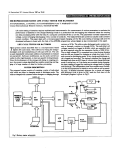
CHAPTER III
CRACK IDENTIFICATION SYSTEM HARDWARE
The three basic hardware components of the initial
configuration for the crack identification system are the
optocator, the 68000 DAQ board and the COMPAQ Portable III
personal computer. The optocator obtains a distance
measurement using non-contact lasers. The 68000 data
acquisition board acquires the data from the optocator at a
specified sampling rate, temporarily stores the data in
onboard RAM and performs some preliminary processing of the
data as well as data reduction. Finally, the COMPAQ accepts a
reduced data set and stores it for final processing and
analysis.
3.1
Optocator
The optocator is an optoelectronic measurement system
which measures the distance to an object with high speed and
prec1s1on. Most importantly, the measurement is made without
contacting the measured surface. The basic components of the
optocator are the non-contact laser probes, the probe
processing units (PPU), and the CPU sub-rack which contains
the power supply and the receiver-averaging boards which
receive and process data from the gauge probes. A laser probe
and probe processing unit are shown in Figure 3.1.
The gauge probe contains a pulsed, modulated (32KHz) and
intensity-controlled laser diode, a position sensitive
photodetector and an appropriate lens system. The laser diode
is a class III b gallium-arsenide (GaAs) laser which entails
the risk of eye damage if the beam hits the eye directly [4).
The GaAs laser in the gauge probe gives off pulsed,
modulated invisible infrared light as shown in Figure 3.2.
Each pulse in the 16 pulse burst is 350 ns. The bursts occur
at a frequency of 32 KHz which accounts for the 32 KHz data
rate of the serial data passed to the receiver-averaging
board. The light from the laser beam passes through a lens
which focuses the light in the center of the measurement
range. The spot size which strikes the ground surface is
approximately 1/4 inch by 1/16 inch.
18
19
Figure 3.1
Laser probe and probe processing unit
•..
20
The optocator measures the distance to an object by use
of the triangulation principle, as illustrated in Figure 3.3.
From a light source, L, a concentrated light beam is directed
onto the surface of the measured object, 01. The light beam
will strike the surface at point A and the scattered light
reflection is focused through a lens to a point A' on a
position sensitive detector. If the distance of the measured
object is changed by X, the laser beam will hit point B on
surface 02 and be focused at point B' on the detector. Since
the relative position of the light source, the lens and the
detector are fixed, the relation between X and X' is known and
distance measurements can be obtained.
The maximum measurement range, 01-02, as well as the
standoff distance must be considered when mounting the laser
probes. Selcom's gauge probe type 2008 requires a standoff
distance of 355mm (13.98 inches) and has a measurement range
of 256mm (10.08 inches) [5]. Therefore, to obtain correct
measurements, the laser probes should be mounted such that the
distance from the bottom of the probe to the ground surface
(middle of the measurement range) is approximately 14 inches.
When correctly mounted, distances plus or minus 128mm (5.04
inches) from the calibrated ground level can be accurately
measured. Refer to Figure 3.4.
Measured surfaces which do
not fall within the measurement range will result in invalid
readings.
The PPU processes the analog signal from the laser probe.
It applies bandpass and anti aliasing filters to the signal.
The PPU converts the analog signal into a serial digital form
which can be transmitted over long distances to the receiveraveraging boards located in the CPU sub-rack. The serial
digital output includes the 12 bit value from the analog to
digital converter as well as 3 invalid data bits. The probe
processing unit determines invalid data if the reflected laser
beam is not correctly detected by the position sensitive
detector in the probe. For example, if the measured surface
is out of the measurement range, the invalid data bits would
reflect this and the data could be processed accordingly.
Another function of the PPU is to control the intensity
of the laser light emitted by the GaAs laser diode in the
probe. This is done through a feedback mechanism.
The receiver-averaging boards are located in the CPU subrack as shown in Figure 3.5. There is one board for each
laser probe. Each board receives serial data from the gauge
probe at a rate of 32 KHz and is capable of reducing the data
rate by forming the average of a number of measurements. The
data rate, also referred to as updating frequency, is set by
jumpers on the board. The update frequency ranges from a
maximum of 32 KHz (no averaging) down to 62.5 Hz in powers of
21
31.25 usee
16 pulaes
Figure 3.2
16 pulaea
16 pulaea
Pulsed, modulated infrared light from GaAs lasers
22
x·
L
01
A
02
I
X
•.
B
Figure 3.3
Triangulatio n principle
23
LJ
STANDOFF
RESOLUTION
(13.98 IN.)
2.44 mV
MEASUREMENT
RANGE
-
(10.08 IN.)
(0-10 VOLTS)
GROUND LEVEL
Figure 3.4
Laser measurement range
·-
two.
Output from the receiver-averaging boards i~ the mea~ured
value represented as 12 bit parallel da+a plus a data
invalid bit and a data ready flag.
This 12 bit p3rallel data
value is input to the 68000 data acquisition board (DAQ) which
interfaces to the COMPAQ's PC bus.
di3~ance
3.2
68000 DAQ Board
The data acquisition board initially used to determine
the measuring characteristics and capabilities for the project
is a specially designed board which uses the Motorola 6800u
processor and plugs into one of the system expansion slots in
the COMPAQ Portable III expansion module (See Figure 3.6).
Its function is to receive the laser data from the optocator
and perform some preliminary processing of the crack data
before passing it on to the COMPAQ Portable III for final
crack identification and section analysis.
The DAQ board is actually made up of two boards.
Schematics for the boards are included in Appendix A.
The
main board contains the M68000 microprocessor, static RAM,
EPROM, serial and parallel I/0 and is capable of running
independently of the other.
The second board is an auxiliary
memory board which only contains buffers and an additional
512K of static RAM.
This board is used when large amounts of
data needs to be stored in real-time.
The main DAQ board features include an 8 MHz Motorola
68000 microprocessor, 64K static RAM, 64K EPROM; two Motorola
68230 parallel interface and timer chips, an Intel 8251 USART
and the IBM PC interface.
The 8 MHz M68000 provides 500 nanosecond bus cycles.
The
static RAM and EPROMs have 100 and 200 nanosecond access time,
respectively.
This allows memory reads and writes with no
wait states.
THe M68230 PI/T chips are programmed in the 16bit port mode to provide the parallel interface for two
lasers.
The timers on the M68230 provide interrupt signals at
the required sampling rate.
The Intel 8251 USART gives an RS232 compatible serial interface running at 9600 BAUD.
The
serial interface is used for most of the communications
between the DAQ and the COMPAQ.
The IBM PC interface provides
an 8-bit parallel interface for downloading large amounts of
laser data to the COMPAQ.
3.3
COMPAQ Portable III
The COMPAQ Portable III is the user's interface to the
entire system.
From the COMPAQ's keyboard the user can run
diagnostic checks on the system, collect a specified amount of
25
Figure 3.5
CPU sub-rack with power supply and receiveraveraging boards
26
data, download crack data to the COMPAQ for storage and
subsequent processing, or enter a real-time crack counting
mode.
The programs which provide detailed crack identification
and section analysis reside on the COMPAQ. When the user runs
a section of road to be analyzed, the data is collected on the
DAQ boards and then downloaded to the COMPAQ for off-line
analysis.
The real-time crack count mode provides a rough estimate
of the number of cracks seen as the van moves at highway
speeds. This estimate is performed by the DAQ board using a
variance measure.
In this mode the COMPAQ is used to issue
the command to the system and to display the crack count.
Figure 3.7 shows the system as it is currently running in
the profilometer.
27
Figure 3.6
Data acquisition (DAQ) boards
.
'J
.
.
-~
'
.L
Figure 3.7
Crack system in the profilometer
CHAPTER IV
TIME AND FREQUENCY ANALYSIS TECHNIQUES
This chapter provides some of the basic concepts in the
theory of time series analysis needed in the processing of
crack data. Most important among these are the concept of a
stochastic process, a stationary process, the autocovariance
function of a stationary process, the frequency content of a
time series, and linear parametric models. Several classical
texts are included in the bibliography and may be referenced
for a more detailed treatment of the subject [11,12,13).
It should be noted that all equations given in this
chapter assume real-valued time series. Since complex-valued
time series are not considered, the complex conjugation
operator needed for the strictest definition of
autocorrelation and autocovariance has been omitted.
4.1
Time Series
A signal which is continuous in time is a continuous time
series. A discrete time series is simply a sequence of
measurements or observations taken at specific instants of
time. Often a discrete time series is a sampling of a
continuous time series. Typically th~ observations are taken
at equispaced time increments and denoted x(n).
A continuous time series may be obtained by measurements
taken from a physical instrument. Such a series is bandlimited and contains no frequencies higher than the maximum
frequency response of the measuring instrument. To analyze a
continuous time series in discrete form the sampling interval
must be determined such that all information present in the
original signal is maintained. This sampling rate must equal
or exceed twice the highest frequency present in the signal
and is generally referred to as the Nyquist rate [14].
A signal from which the series was obtained could be
deterministic or stochastic in nature. If it is possible to
predict future values of the series exactly, the signal is
deterministic. If future values can only be approximated
based on statistical characteristics of past observations, the
signal is a statistical or stochastic time series.
28
29
4.2
Stochastic Process
The possible values of the time series at a given time t
are assumed to be described by a random variable X(t) and its
associated probability distribution. An observed value x(t)
at time t represents one of the infinite number of possible
values of the random variable X(t). The probability
distribution function F(x(t)) defined by F(x(t)) = Prob(X(t) <
x(t)) is the probability that random variable X(t) has a value
less than or equal to x(t).
The behavior of the time series at all sampling times is
described by an ordered set of random variables {X(t) ). The
statistical properties of the time series are described by
associating a probability distribution function with each
random variable in the set. The ordered set of random
variables {X(t)} and the associated probability distribution
functions is called a stochastic process. An observed time
series x(t) is only one of an infinite number of possible
realizations of the stochastic process. Th~ collection of all
sequences that could result as realizations of the stochastic
process is called an ensemble of sample sequences.
The expectation of a random variable X(t) at time t,
denoted by E{X}, is given by
E{X}
f x p(x) dx =
J
x
Here x is the observation at time t and p(x) is the
probability density function of X(t). This implies that the
mean, x, is based on values x taken from all possible
ensembles of the random variable at time t.
The expected value of the squared magnitude of random
variable X is
E{jXI 2 }
= J lxl 2
p(x) dx
-~
is the mean squared value of X.
The variance of a random variable is the mean squared
deviation of the random variable from its mean,
30
var{X}
=
r
J
lx- E{X}I 2 p(x) dx
-m
An indication of the statistical relationship of one
random variable Xl at time tl to another X2 at time t2 is
given by the autocorrelation
r{X1X2} = E{X1X2}
This represents the engineering definition for
autocorrelation, as first suggested by Weiner. The
autocorrelation of a stochastic process with the mean removed
is the autocovariance, given by
c{XlX2}
=
E{(Xl- E{Xl})
=
r{XlX2} - xl x2
(X2- E{X2})
If the random process has zero mean for time tl and t2 then
c{X1X2} = r{X1X2}.
Also, if the random variables Xl and X2 are mutually
independent or uncorrelated then
c{X1X2}
=
0 .
This implies that there is no relationship between the two
random variables and knowing values for Xl does not help in
predicting a value of X2.
4.3
Ergodicity and Stationarity
The definitions of mean, variance, autocorrelation, and
autocovariance described above are based on statistical
ensemble averaging. That is, they were based on observations
at a particular time t.
In practice one does not have the
luxury of an ensemble of waveforms from which to evaluate
these statistical descriptors. Typically these statistical
31
estimates are obtained from a single waveform x(n) by
substituting time averages for ensemble averages. Here x(n)
represents a discrete time series. For a stochastic process
to be accurately described by time averages instead of
ensemble averages the process must be ergodic. Ergodicity
requires a certain amount of stationarity; that is, the
statistics must be independent of the time origin selected.
A random process is wide sense stationary if its mean is
constant for all time indices and its autocorrelation depends
only on the time index difference m, where m=n2-n1. The
variable m denotes the time lag, that is, the number of time
increments between time n2 and time n1.
All results reported in this study assume the data is
wide sense stationary or at :east locally stationary such that
time averages can be substituted for ensemble averages.
4.4
Statistical Estimates
If a stochastic process is ergodic then
E{X1} = E{X2} = E{X3} =
= E{XN}
and the mean, x, can be estimated by
X
= 1/N
N
E
x(n)
n=1
The autocorrelation and autocovariance functions no
longer depend on the time index of the random variable, only
the time index difference. The time index difference is
referred to as the lag and denoted by m. The autocorrelation,
r, and the autocovariance, c, then become
r(m) = E{x(n+m) x(n)}
and
c(m) = E{(x(n+m) - x)(x(n) - x)}
=
r(m) -
x2
Assuming ergodicity, the autocorrelation and autocovariance
can be estimated by
32
N-m
r(m) = 1/(N-m)
E
x(n) x(n+m)
n=1
and
c(m) = 1/(N-m)
4.5
N-m
Z
n=1
(x(n) - x)
(x(n+m) - x)
Power Spectrum Estimation
Spectral analysis is any signal processing method that
characterizes the frequency content of a measured signal.
In
spectral analysis one is typically interested in obtaining a
spectral plot which represents the distribution of signal
strength at each frequency.
Peaks in the spectral plot show
which frequencies are predominant in the signal. Most power
spectrum estimation is accomplished by either the
autocorrelation or the direct method [15]. The latter method
has become the most popular because of the fast Fourier
transform (FFT) algorithm developed in 1965 [16]. The FFT is
a fast, efficient algorithm for computing the discrete Fourier
transform (OFT) of a time series. The OFT determines a
sampled periodogram in which the values of the periodogram for
only a discrete number of equally spaced frequencies is
computed rather than evaluating over the continuous range of
frequencies.
The method for calculating the power spectra in this
study was first proposed by Welch [17]. This method segments
the data, applies a window to each segment, determines the
periodogram of each windowed segment, and then calculates the
average periodogram, which is called the modified periodogram.
With this method the data segments may be overlapped. This
method of periodogram averaging reduces the variance of the
spectral estimate.
The essential features of this method are described
below. The available time series x(n), 0 < n < N-1, is
divided into K overlapping segments of length L. The segments
overlap by L/2 samples. The total number of segments then
becomes
K
=
(N - L/2)/(L/2)
where any fractional portion of K is truncated.
segment then becomes
The ith data
33
xi(n)
x(iL/2 + n) w(n)
=
where 0 < n < L-1, 0 < i < K-1 and w(n) is a window function
of length L.- Typically, eithe~ a rectangular or Hamming
window is used.
The DFTs of each of the K data segments are then computed
using the FFT algorithm by
M-1
xi (k) = E
n=O
xi(n) exp(-jkn(2W/M))
where 0 ~ k ~ M-1 and 0 < i < K-1.
must be > L.
M is the DFT length and
The modified periodograms, Si(k), are then averaged to
produce the spectrum estimate
for 0 < k
S(2~k/M)
= 1/KU
~
~
M-1, 0
K-1
E
i=O
Si(k)
i < K-1 and
Si(k) = IXi(k) 12
and
U =
4.6
L-1
!
n=O
w2 (n)
Linear Parametric Modeling
Many discrete time stochastic processes can be
approximated by a linear regression model. In this model, the
input driving white noise series w(n) and the observed output
time series x(n) are related by the linear difference equation
34
x(n) = b 0w(n) + b 1w(n-1) + ... + bqw(n-q)
- a 1 x(n-1) - ... - apx(n-p)
This may be rewritten in the form
p
x(n) =
q
E aix(n-i) + . E b·w(n-i)
1
i=1
1=0
This general regression model is called an autoregressivemoving average (ARMA) model.
If all ai = 0, then
q
x(n) =
.
~
1=0
b·w(n-i)
1
and the process is known as a moving average model of order q
and represented MA(q).
If all bi = o, i > o, then
x(n) = -
p
E
.
1=1
a·x(n-i)
+ b 0 w(n)
1
and the process is known as an autoregressive model of order
p; that is, AR(p).
Any one of the three parametric models described above
may be expressed in terms of the other two models. An ARMA or
MA model of a finite number· of parameters may be described by
an AR process, generally of infinite order. Similarly, an
ARMA or AR process can be expressed as a MA model of infinite
order. This observation is important because it suggests that
any of the three models may be selected and a reasonable model
obtained if a sufficiently large order is used. Of the three
models, the AR model has mathematical characteristics which
have allowed the development of a number of efficient
algorithms. Specifically, AR models have linear solutions;
whereas, solving for ARMA or MA parameters involves nonlinear
equations.
35
Estimates of the AR parameters ai can be obtained as
solutions to the p+1 linear equations given by
r(O)
r{-1)
r{-p)
r(1)
r{O)
r(-p+1)
1
0
=
r(p)
r(p-1)
r{O)
0
These linear equations are commonly referred to as the YuleWalker equations. The autocorr;lation matrix is both Toeplitz
and Hermitian because r(-k) = r (k), where* represents
complex conjugation. These properties allow more efficient
solution than the standard Gaussian elimination. The method
for solution of the Yule-Walker equations that takes advantage
of these properties was developed by Levinson and is commonly
referred to as the Levinson-Durbin algorithm [31,32].
CHAPTER V
ANALYSIS OF PAVEMENT CRACKING DATA
5.1
Introduction
The methods first investigated to identify pavement
cracking are computationally intensive and cannot be performed
in real-time with the hardware developed in this study. Each
of these methods involve first filtering the data and then
applying various statistical techniques to identify cracking.
Data is filtered to remove the low frequency content of the
signal. Low frequency components include such things as wheel
bounce, vehicle suspension effects, bumps and hills in the
section.
The two methods which consistently gave best results were
the running meanjslope threshold technique and the
autocorrelation difference method. These are discussed in
detail in Sections 5.4 and 5.5, respectively. Another
technique considered was modeling the data as an AR process
and then examining the AR coefficients. This method would
allow crack identification and classification if each cracking
type would give distinctly different AR parameter values and
the same type cracking would give similar coefficients. The
AR modeling results are discussed in Section 5.6.
As stated, the methods mentioned above give detailed
analysis and cannot be performed in real-time with existing
hardware. It was desired to develop a technique, even a rough
estimate, which could perform in real-time with the hardware
described herein. A technique, using a variance measure, has
been implemented which provides a crack count in real-time.
This is discussed in the following section.
5.2
Variance Method for Real-Time Crack Counting
Although detailed crack identification and classification
cannot be obtained using the DAQ board and COMPAQ at highway
speeds, an estimate of the number of cracks seen is possible
using a simple variance calculation. This method simply
calculates the variance every 16 data points (1 inch) and
compares that statistic to a threshold level provided by the
operator. If the variance for that inch of data surpasses the
36
37
threshold, the count is incremented and displayed on the
COMPAQ. This calculation takes approximately 40 ~icroseconds
on the DAQ board, well within the 71 microsecond requirement
for 50 miles per hour.
The variance is calculated on 16 raw data values. Since
unfiltered data is used, there exists ·variance in the data due
to the factors previously mentioned which contribute to low
frequency content of the signal. However, because. only 16
data points are used in each calculation these components do
not contribute as heavily to the variance value as high
frequency cracks and thus filtering can be neglected to save
calculation time.
The accuracy of this technique is highly dependent upon
the operator entering meaningful threshold values. More
investigation is needed to determine reasonable threshold
limits for various pavement textures.
5.3
Spectral Analysis Results
Typically, one of the first things that should be
considered about any measured signal is its frequency content.
As previously discussed, spectral analysis provides this
information. Of particular interest in this study was a
determination of whether or not the different cracking types
displayed characteristic power spectra. Also, it seemed
reasonable that cracking of the different severity types might
show characteristic peaks at different frequencies. The
procedures described below provide information about the
frequency content of pavement cracking data.
The first question addressed was whether or not each
cracking type had its own characteristic spectrum. Here
several data segments of 1000 data points in length were
identified from the test sections for each of the desired
types. The types considered were moderate alligator, moderate
block, and no cracking. Moderate transverse cracking was not
included because by using 1000 data points (5.2 feet) a single
crack may or may not have been seen in the data; thus, it
would appear as block or no cracking. A typical power
spectrum for these three types is shown in Figure 5.1. Three
important observations can be made from that figure.
First, no cracking appears as virtually a straight line.
There are no frequencies or range of frequencies which are
predominant. A flat power spectrum indicates white noise:
that is, the signal is completely random and there is no
correlation in the data. A second observation is that data
with cracking shows no noticeable peaks at any frequencies but
does consistently show more power at the lower frequencies
(greater than 1/4 inch wavelengths). This suggests that data
38
with cracking is correlated and statistical measures such as
autocorrelation and autocovariance will be appropriate.
Finally, moderate alligator shows more power than moderate
block at the low frequencies. This implies that more cracking
means more correlation of the data and larger autocorrelation
and autocovariance values should be observed.
Figure 5.2 shows typical power spectral results for
sections with moderate versus severe alligator cracking.
Initially it was felt that perhaps different severity (widths)
of cracking might show peaks at different frequencies. This
has not been observed. However, consistent with previous
results, a higher degree of cracking again shows more power at
wavelengths less than 1/4 inch. Slight alligator cracking was
not included because it is not believed that the lasers are
accurately measuring slight (less than 1/8 inch) cracks.
In summary, the spectral analysis results indicate that
data obtained from road pavements with no cracking is
uncorrelated. Data from pavement with cracking is correlated:
in fact, the higher the degree and severity of cracking, the
more correlated the data is.
5.4
Running Mean/Slope Threshold Method
The basic idea behind this method is that a running mean,
representing ground level, is maintained and each new data
value is compared with this mean to determine if it is a value
taken from a crack or not. The term running is used because
the mean must be constantly updated using the new data points
to maintain an accurate representation of ground level. Data
points which are determined to represent a crack or a surface
too much above ground level, perhaps an extraneous rock or
spikes in the data, do not contribute to the running mean
calculation. The running mean is an average calculated from
the last N data points which have been determined to be at
ground level. N is user selectable, typically 4 to 8.
The simplest way to apply this technique is simply to
compare each new data value to the running mean. If it is
below a threshold distance from ground level then identify it
as a crack, do not include it in the mean, and advance to the
next point. If it is less than a threshold distance below the
running mean then it is not a crack and the value replaces the
"oldest" value used in the mean calculation and a new running
mean is determined. Unfortunately this will not provide
accurate crack identification for cracks with gently sloping
walls. The problem is that although the values are decreasing
they may not exceed the threshold using the technique
described above and so they are included in the running mean.
This lowers the mean value and makes it even more difficult
for the next point to be identified as part of a crack. The
39
100
90
eo
70
,......
60
.0
'0
""
0
50
lo'l
n.
-40
.30
20
10
0
0
a
0.062
0.125
0.187
0:.25
0.312
O.J75
0.437
0.5
FRACTION OF SAWPUNG FREQUENCY
No Crocking
Figure 5.1
+
Wod. Block
<>
Wod. Alll9ator
Power spectral.density plots of different cracking
types
,J
100
90
80
70
,...._
60
.0
't!
'-"
a
50
Ill
0.
40
30
20
10
0
0
0.062
0.125
0.187
0.25
0.312
0.:!75
0.437
05
FRACTION OF SAMPUNG FREQUENCY
0
Figure 5.2
I.Cod. Alligator
+
Sev. AJii9<Ji:or
Power spectral density plots of different cracking
severity
41
problem is solved by looking ahead up to L lookahead points,
assuming all values are constantly below the mean, for a value
exceeding the threshold before updating the running mean. L
is a user supplied parameter. If the threshold is exceeded
within L points, then each of the decreasing data points are
identified as part of a crack and will not be included in the
mean.
The accuracy of this method depends on the number of data
points used in the mean, the number of data points allowed in
the lookahead for threshold violation, and the threshold value
itself. After plotting and examining results from various
types of cracking in the test sections, it is believed that
about 85% of the cracking can be identified using 4 points for
the mean and lookahead value and 35 for a threshold level.
This technique performs better if the data is first
filtered to remove the DC component and longer wavelengths.
highpass Butterworth filter is typically applied to the raw
data.
A
Figures 5.3 and 5.4 show the results of applying this
algorithm to moderate and severe alligator cracking,
respectively. 1000 (5.2 feet) filtered data points have been
plotted in both figures. Above the filtered data is a plot
representing whether or not a crack has been seen. Ground
level is plotted at 200 on the Y-axis and cracks at 100.
The running meanjslope threshold algorithm is included in
Appendix B.
5.5
Autocorrelation Difference Method
The autocorrelation is a statistic which measures the
correlation of data at different time increments apart.
Assuming ergodicity, the autocorrelation lag m, denoted r(m),
tells if data points m time increments apart over a length of
data are related. The autocorrelation value will be
approximately zero if the data is uncorrelated. As shown by
the power spectral analysis results of Section 5.3, data with
cracking is correlated. Data with sharp cracks will show
large correlation for a lag or two but the autocorrelation
value decreases rapidly as the number of lags increases. Data
with longer wavelength components, such as bumps, show high
autocorrelation values for longer lag times.
Section 5.2 discussed a "quick and dirty" way of
identifying cracks in unfiltered data by calculating the
variance, c(O), every 16 data points and then comparing that
value to a threshold. That method was, at best, an estimate.
However, because the data was not filtered and only a simple
variance calculation was needed, it did meet the real-time
42
1000 DATA POINTS
Figure 5.3
(5.2 FT.)
Running mean/slope threshold technique applied to
moderate alligator cracking data
43
~0,-------------------------------------------------------~
400
300
100
-100
-200
-300
-400
-000,_. . . . . . . . . . . . . . . . . . . . . . . . . . . . . . . . . . . . . . . . . . . .. . .
1000 DATA POINTS
Figure 5. 4
(5.2 FT.)
Running meanjsl·ope threshold technique applied to
severe alligator cracking data
44
requirement. The autocorrelation difference method is an
enhancement of the simple variance method. Using this method
the data is first filtered with a highpass filter. Filtering
removes the DC component and much of the variability caused by
hills, tire bounce, and vehicle suspension effects. This can
be seen by comparing the raw data plot in Figure 5.5 with the
plot of filtered data in Figure 5.6. With the DC component
removed, the data now approximates a zero mean process and the
autocorrelation lag 0 is an estimate of the autocovariance lag
o which, by definition, is the variance.
The autocorrelation difference method involves
determining the spread between r(O) and r(m) calculated for
every one inch (16 points) block of data. This difference is
then compared with a threshold value. As discussed
previously, r(O), an estimate of the variance for zero mean
data, is large for data with cracking. r(O) will also be
large if the data varies too far from the zero mean as is the
case on a rough road when the filter is not able to keep the
data sufficiently close to a zero mean. This is illustrated
in the last 100 data points plotted in Figure 5.6. r(m) is
the autocorrelation for data points in the 16 point block
which are m time lags apart. r(m), m is typically 4, will
decrease more rapidly if variance in the data is higher
frequency, that is, sharp cracks.
Using the property r(O) ~ r(m) and exam1n1ng the four
cases for relative values of r(O) and r(m) provides
justification for this technique.
CASE I:
r(O) small and r(m) small implies a small
difference and no cracking.
CASE II:
r(O) small and r(m) large is not
by property r(O) > r(m).
CASE III:
r(O) large and r(m) small implies a large
difference and cracking present.
CASE IV:
r(O) large and r(m) large implies a small
difference and no cracking.
possible
Figure 5.6 shows filtered data with the r(O)-r(4) value
plotted over the sixteenth point of each block of data. Also,
any difference greater than 1000 is plotted as 1000 so all
information could be plotted on a reasonable scale. As can be
seen from the plot, a threshold of 200 identifies all cracks
except the one at point A on the plot. Here a shortcoming in
the algorithm is illustrated. That is, when one 16 point
block ends and another begins in the middle of a small crack
it may not be detected.
45
3
2.9
2.8
2.7
2.6
2.5
........
2.4
~ ~
2.3
wIll
:::l-o
...J c:
0 ~
';{~
'-/
2.2
2.1
2
, 9
1.8
1. 7
1.6
, .5
1000 DATA POINTS
Figure 5.5
(5.2 FT.)
Raw data
.
46
Figure 5.6 and 5.7 taken together illustrate each of the
cases described above. Figure 5.6 shows the difference r(O) r(4) while Figure 5.7 shows the actual values of r(O) and
r(4)'. For example, Case III was large r(O) and small r(4).
The actual values are plotted in Figure 5.7 and then Figure
5.6 can be examined to see the characteristics of the data and
the actual difference value.
The autocorrelation difference method has been applied to
several of the test sections with good results. In fact,
cracking identified by this method compares favorably with
that identified by the running meanjslope threshold method.
One drawback of this method, however, is that it will not be
able to accurately detect crack width.
5.6
AR Process Modeling Results
This technique was investigated to determine whether or
not the coefficients obtained by modeling crack data as an AR
process could successfully be used to classify cracking types
and severity. The assumption was that cracking of the same
type and severity would show similar coefficients while the
coefficients would be significantly different for a different
type and/or severity of cracking.
First, several sections of test data were modeled to
determine the number of coefficients to use. It was found
that only the first three coefficients contributed
significantly; that is, beyond three lags the coefficients
were essentially zero. This was also substantiated by the
fact that the variance of the white noise, the error term,
could only be decreased to a certain level by adding AR terms;
beyond that, it really did not improve the model by adding
additional terms.
Having determined that three terms should be used in the
model, different types of cracking were then examined. Blocks
of data one foot in length were examined. It was found that
data with more cracking showed higher autocorrelation values
and the coefficients were significantly larger than data with
no cracking. However, the resolution required to provide the
detailed information needed simply was not there. This
technique could tell if there was a large amount of cracking
or little to no cracking in each one foot block, but that was
all. Since the details, such as approximate number of cracks
or severity, could not be ascertained, this method was not
considered further.
47
1.1 -,----------------------------------------------------------~
+ +
0.9
+
+~
o.e
Case III
0.7
....
'""'
'0
0.6
t:
0.5
"
0.4
0
:I
0
(::.
'-"
+
0 ..3
+
0.2
0.1
+
+
+
+
Case IV
+
+
+
0
-o.1
-o.2
1000 DATA POINTS
Filtered Dole
Figure 5.6
(5.2 FT.)
+
r(O)-r( 4)
Filtered data with r(O)-r(4) value plotted every
16 data points
.
48
2.2
c
2
c
, .8
, .6
t;:
, .4
Case IV
, .2
Case III
.-..
"c
"1:7
0
0.8
:I
~
.....,
0
!i1
0.6
c
0.4
+
0
c
0.2
c
oc
+
0
+
-Q.2
-Q.4
-o.6
-o.e
+
a
Figure 5.7
+
/
a
VI
0
0
----;lo
r(o)
+
r(4)
Actual r(O) and r(4) values for the data in
Figure 5.6
I
CHAPTER VI
CONCLUSIONS AND FURTHER RESEARCH
The report describes the first two phases of research
Project 8-18-86-1141 for developing an automated method of
obtaining and evaluating pavement distress and cracking
information for PES. For these initial two phases, the use of
two lasers, one in each wheel path, are used to obtain
cracking data which is processed on a Motorola 68000 based
data acquisition board and the COMPAQ Portable III. For
detailed analysis, the data is filtered to remove the DC
component and long wavelengths before processing. The data is
analyzed using several different statistical techniques. Two
techniques in particular have been shown to be very reliable.
These are the running meanjslope threshold and the
autocorrelation difference methods. Software still needs to
be written which take the results from these two methods and
provide the detailed reporting, that is, the percentage and
severity of each cracking type within the section.
Several important conclusions can be made as a result of
this initial study. First, alligator and block pavement
cracking can be detected using the Selcom lasers n~Junted in
the wheel paths. However, it is unlikely that transverse
cracking can be accurately identified. It is believed that
additional lasers must be installed to obtain data across the
lane before the system will be able to provide this
information. Using only two lasers it is simply too likely
that something in 30 to 50 feet of data will appear to be a
crack even on smooth pavement. With multiple lasers,
transverse cracking would be identified only after each laser
across the lane had detected a crack within the same foot or
two of data. It should perhaps be pointed out that multiple
lasers would also allow rutting to be detected. Recall,
rutting is one of the seven distress types currently reported
by PES. Three lasers are being investigated in Phase 3.
Another issue which remains unresolved is whether or not
slight (less than 1/8 inch) cracking is accurately detected.
The old lasers with 3/8 by 1/8 inch spot size could not detect
them. The new lasers with 1/4 by 1/16 inch spot size have
performed reasonably well on the laser calibration board but
have not been thoroughly field tested due to the forementioned
problems.
49
50
Any user of this system must understand the limitations
imposed by trying to detect cracking using only two narrow
beams of laser light running parallel to the centerline.
Obviously, massive amounts of information across the lane is
not available. Due to the nature of the sensors used, cracks
detected in failures and longitudinal cracking patterns will
be misclassified as alligator or block cracking. There is
little that can be done to prevent this using lasers as
sensing devices. The distress types such as failures,
patching and longitudinal cracking can only be detected if the
entire lane is examined using video cameras as described by
other researchers [6,7]. Video system provide much more
detail, but this extra detail presents problems in processing
out the unwanted information. A system with a small cluster
of lasers along and in between each wheel path would seem to
provide the best choice, however, would likely be to costly.
As pointed out numerous times, the algorithms developed
for detailed identification and analysis cannot be performed
in real-time with the hardware developed in this initial
study. Prototype boards which are wirewrapped, such as the
DAQ board built for this project, are limited to clock speeds
less than 10 MHZ because of noise problems, regardless of the
maximum clock frequency allowed. Therefore, to obtain faster
speeds, printed circuit boards must either be built or
purchased. Also, to obtain more computing power a 32-bit
microprocessor should be considered over the 16-bit 68000.
It is believed the open architecture VMEsystem developed
by Motorola should provide needed hardware upgrades for this
project. The VMEsystem allows the user to purchase a basic
cardcage which has the VMEbus interconnect standard. The user
can then configure the system for his specific needs by
purchasing individual VMEmodules which simply plug into the
VMEbus with the widely accepted eurocard connector. Typical
VMEmodules are microprocessor boards, memory boards, various
controller boards, and I/O boards. The VMEsystem architecture
allows the user to configure a multiprocessor system with both
local and shared memory.
A multiprocessor VMEsystem is currently being assembled
for this project. For this system VMEmodules with the 68020
microprocessor interface to the PC. Each of these VMEmodules
will be dedicated to processing the data from a single laser.
This system should provide the computing power needed to
filter the data and identify cracking, at least with the
autocorrelation difference method, in real-time.
It is still questionable whether or not the running
mean/slope threshold method, which provides severity
information, will run in real-time. It may very well be the
case that the data will be filtered and cracks identified in
51
real-time but severity information obtained off-line from a
reduced data set stored on the COMPAQ. If a reduced data set
is required, data compression techniques will need to be
investigated further.
Several other methods are yet to be investigated, which
may aid in identifying cracks. Once specific algorithms have
been identified, the generality of the 68020 microprocessors
may not be required and a system using special purpose signal
processing chips may be possible.
APPENDIX A
DAQ BOARD SCHEMATICS
52
53
____
._:~
••II
L
c
;·--I
("' , ,.I
... "'i
c
•
I
2: I
~~~~,~~:-')
i:
I
·~·
!,_:,
::::
'
..,, '
~
'•'.,
~ Cl~~~
:fr.l""',
-~,-1!
~~·-j
.~1~ ~~~~~~~~il';l~l
~,,&lll~i~l::.: ~
i"l-i
4,< . . 1............ 1-.-a..
I
I
~
:
I!
~I
·-
II
54
Ui1
71l :;:! 1'1
_j~
~~~··~ ::R]~
~~;J.,
~~- --=-~1:~;
;~;~-,,
-!:!~:}fi:S~~·---py,; -~
r-~1~'(1 .~;,"' -~i r~
±ill:;;
cr-:;_,._~J~~:3,:
Plt~.!-J:.J£......."
... _ _
P::
P:l
~~
,... ~
r"''
7
b'
1,_.
•" ,i3
_., l
·'
::z~= I Jjr±~~;;~ ::~h:ii!Gr~;J;t=j 1o
•a•r-.
-r__j~~~~-" ·"'~'li:'I-J.l_
p~ ,,---t::::::'J I t G •r · ll,•iiU;
1 ___.;...J
PR"
.
., •:·~wJ
pp;
PH
..
8=--:=
l
..
w~· lC-.
-----l.l.1:: t,l-::4
·
~ c.:J
• r:• :;;.::_.
~' r::"' ~
1
li====::liJ'',
'"'"'-- .___:,; :r~
..LtJ 1 ' ~ ::~fi_ __ _..u; Cl"
::.:~o:
Pr,:PlRU'~i:IIIP'
iJL
PL~.'PU,.~
F!: 1 -
_
-
T·•L!Tlf:
Pll:T"l!!~!-----
;,.~
._.:_j
ll c:<
1
..~....
·'"<. :-:--1'
I_C"'' '.
. - -' ..
:·:1 ZRlt~-L-- ~ c:: Z..-.f
, .. ' -~
~- - a··~··~· -
H l
Pf':,·..
:..~~_.
Jl·:
,~~;
•• .II.
I L-:J c 3:
;
7iL::.=:H
fr;:l!Rc.,jlL
I
-
•_•'
ri'~:------~:·.<.A\<
'"]
c; ""] ••
PH
I
1!-~
PR>~- I 1_;!J4 lll!~c.t
IJ.:-~1
i'~t:•. ,...._.
P;;:-~ --~~~
...L:.i::~
I"
:;J
';J!'
:r
1
lJ [),
.
,L..,.
1
.:J.~~
'
~
*1;,,
•
.. ·
c· ... ~
~~ :14--
''":
•IiI
---~
·~lr
G
U1
U1
56
57
----------~---------1__--------~--------~~--------~----------L·---------c=----r~-.T~
"'
~
'
i"
i
I
•j·
4'..1
I
I
~I
~r
I
I
;I
"
I
·~I
~~
'-
I
.H
..
58
-~------- ·--e
I
II
I I
II
I
l
·:!.;;t
-
!
I
·--I
!I
IL
·I t·•
:n
APPENDIX B
RUNNING MEAN/SLOPE THRESHOLD LISTING
59
60
C******************************************************
c
c
c
c
c
c
This program inputs a filtered data file and
detects cracks using the running mean/slope
threshold method described in Chapter V.
C
C
FILEIN - input data file
FILEOUT - output file containing crack info
c
for plotting
c
XM - array of X values used in current mean
c
XD - array of X values used in lookahead if
c
values are decreasing
C
XU - array of X values used in lookahead if
c
values are increasing
C
M - pointer into XM array
c
D - down counter
c
U - up counter
C
DX - value output to file for plotting cracks
C
200 = ground level
c
300 = above gnd level (spikes or errors)
C
100 = crack
C
C - counter of number of points in crack
C
if > 96 (6 11 ) will reset
c
IC - same as C but above gnd level
c
NPTS - number of data points
c
NPTSXBAR - number of points to use in mean
C
MTHRESH - threshold value
c
NBASE - number of lookahead points
C
XBAR - running mean
C*******************************************************
PROGRAM RMST
CHARACTER*24 FILEIN,FILEOUT
DIMENSION XM(8),XD(8),XU(8)
INTEGER U,D,IC,C
WRITE(*,*) 'Input file for detect? '
READ(*,901) FILEIN
901
FORMAT(A24)
WRITE(*,*) 'Output file for detect? '
READ(*,901) FILEOUT
WRITE(*,*) 'Number of.data points? '
READ(*,*) NPTS
WRITE(*,*) 'Number of points to use in mean? '
READ(*,*) NPTSXBAR
WRITE(*,*) 'Mean threshold? '
READ(*,*) MTHRESH
WRITE(*,*) 'Slope base length? 1
READ(*,*) NBASE
OPEN(UNIT=2,FILE=FILEIN,STATUS='OLD 1 )
OPEN(UNIT=3,FILE=FILEOUT,STATUS='NEW')
c
c
Initialize XBAR and XM array
61
c
30
c
c
c
c
c
c
c
c
c
100
c
c
c
c
PEAD(2,*) X
XBAR=X
XTOT=XBAR*NPTSXBAR
DO 30 I=1,NPTSXBAR
XM(I)=X
CONTINUE
M=1
DX=200
WRITE(3,*) DX
L=2
U=O
D=O
IC=O
C=O
Loop over all points
DO 500 K=2,NPTS
READ(2,*) X
Check if X going up or down
IF(X.LT.XBAR) THEN
Going down so reset UP counters and arrays
IF(U.NE.O) THEN
IC=O
C=O
DO 100 J=1,U
XTOT=XTOT-XM(M)+XU(J)
XM(M)=XU(J)
M=M+1
IF(M.GT.NPTSXBAR) M=1
DX=200
WRITE(3,*) DX
CONTINUE
XBAR=XTOT/NPTSXBAR
U=O
END IF
Increment DOWN count, store in array and
check if surpasses threshold
0=0+1
XD(D)=X
IF(XBAR-X.GE.MTHRESH) THEN
DO 110 J=1,D
DX=100
WRITE(3,*) DX
C=C+1
62
110
c
C
C
c
120
c
c
c
c
c
CONTINUE
Check if have been in crack too long and
RESET if > 6"
IF(C.GT.96) THEN
C=O
XBAR=X
XTOT=XBAR*NPTSXBAR
DO 120 J=1,NPTSXBAR
XM(J)=X
CONTINUE
M=1
END IF
D=O
ELSE
If were decreasing for NBASE number of
of lookahead points but did not surpass
threshold then update by 1 point and cont.
IF(D.EQ.NBASE) THEN
IC=O
C=O
XTOT=XTOT-XM(M)+XD(1)
XBAR=XTOT/NPTSXBAR
XM(M)=XD(1)
M=M+1
IF(M.GT.NPTSXBAR) M=1
DX=200
WRITE(3,*) DX
DO 130 J=1,NBASE-1
XD(J)=XD(J+1)
130
CONTINUE
D=NBASE-1
END IF
END IF
C**************************************************
c
c
c
c
Similar code as for DOWN but here are going
UP
C**************************************************
ELSE
IF(D.NE.O) THEN
IC=O
C=O
DO 200 J=1,D
C
XTOT=XTOT-XM(M)+XD(J)
C
XM(M)=XD(J)
M=M+1
C
C
IF(M.GT.NPTSXBAR) M=1
63
200
C
c
C
C
c
210
c
c
c
DX=200
WRITE(3,*) DX
CONTINUE
XBAR=XTOT/NPTSXBAR
D=O
END IF
U=U+1
XU(U)=X
Make X surpass 3*threshold before kick out as
data point not to be included in running mean
IF(X-XBAR.GE.3*MTHRESH) THEN
DO 210 J=1,U
DX=300
WRITE(3,*) DX
IC=IC+1
CONTINUE
Checking if need to reset
THEN
IC=O
XBAR=X
XTOT=XBAR*NPTSXBAR
DO 220 J=1,NPTSXBAR
XM(J)=X
CONTINUE
M=1
END IF
U=O
ELSE
IF(U.EQ.NBASE) THEN
IC=O
C=O
XTOT=XTOT-XM(M)+XU(1)
XBAR=XTOT/NPTSXBAR
XM(M)=XU(1)
M=M+1
IF(M.GT.NPTSXBAR) M=1
DX=200
WRITE(3,*) DX
DO 230 J=1,NBASE-1
XU (J) =XU (J+1)
CONTINUE
U=NBASE-1
END IF
END IF
END IF
CONTINUE
IF(IC~GT.96)
220
230
500
c
C
Through all data points, account for any
64
c
c
600
700
data points left in UP or DOWN arrays
IF (U.GT.O) THEN
DO 600 I=l,U
DX=200
WRITE(3,*) DX
CONTINUE
END IF
IF (D.GT.O) THEN
DO 700 I=l,D
DX=200
WRITE(3,*) DX
CONTINUE
END IF
STOP
END
REFERENCES
[ 1]
Walker, Roger s. , Freddy L. Roberts, and W. Ronald
Hudson, "A Profile Measuring, Recording, and Processing
System", Research Report 7 3-2, Center for Highway
Research, The University of Texas at Austin, April
1970.
[2]
Claros, German J., W. Ronald Hudson, and Clyde E. Lee,
"Performance of the Analog and the Digital Profilometer
with Wheels and with Non-Contact Transducers", Research
Report 251-3F, Center for Highway Research, Bureau of
Engineering Research, The University of Texas at
Austin, April 1985.
[3]
Walker, Rogers., and John Stephen Schuchman, "Upgrade
of 690D Surface Dynamics Profilometer for Non-Contact
Measurements", Research Report 494-1F, The University
of Texas at Arlington, December 1986.
[ 4]
11
[5]
"Selcom User's Manual",
(unpublished).
[6]
Cox, Gregory M., Donald Fronek, and Rahn Merrill,
"Real-time Computer Vision Using Intelligent Hardware",
Applications of Artificial Intelligence III, SPIE vol.
635, pp. 564-574, 1986.
[7]
Mahler, David S., "Final Design of Automated Pavement
Crack Measurement Instrumentation from a survey
Vehicle", Report No. FHWA/RD-85/077, Federal Highway
Administration, Washington, D.C., 1985.
[ 8]
"Pavement Evaluation System Rater's Manual", Texas
state Department of Highways and Public Transportation,
1987.
Selcom Technical Manual",
(unpublished).
65
Selective Electronic
Co.,
Selective Electronic Co.,
66
[9]
Epps, J. A., A. H. Meyer, I. E. Lattimore, Jr., and H.
L. Jones, "Roadway Maintenance Evalua.tion User• s
Manual", Research Report 151-2, Texas Transportation
Institute, Texas A&M University, September 1974.
[10]
Smith, Roger E., Michael I. Darter, and Stanley M.
Herrin, "Highway Pavement Distress I dent if ication
Manual for Highway Condition and Quality of Highway
Construction Survey", Federal Highway Administration,
Washington, D.C., 1979.
[11]
Box, George E. P., and Gwilym M. Jenkins, Time Series
Analysis: Forecasting and Control, Holden-Day Inc., San
Francisco, California, 1976.
[12]
Jenkins, Gwilym M., and Donald G. Watts, Spectral
Analysis and Its Applications, Holden-Day, Inc., San
Francisco, California, 1968.
[13]
Papoulis, Athanasios, Probability, Random Variables,
and Stochastic Processes, McGraw-Hill, Inc., New York,
1984.
[14]
Oppenheim, Alan V. , and Ronald W.
Signal Processing, Prentice-Hall,
Cliffs, New Jersey, 1975.
[15]
Childers, Donald G., ed.,
IEEE Press, New York, 1978.
[ 16]
Cooley, J. W., and J. w. Tukey, "An Algorithm for the
Machine Calculation of Complex Fourier Series", Math.
Comput., vol. 19, pp. 297-301, April 1965.
[17]
Welch, Peter D., "The Use of Fast Fourier Transform for
the Estimation of Power Spectra: A Method Based on Time
Averaging Over Short, Modified Periodograms", IEEE
Trans. Audio and Electroacoust., vol. AU-15, pp. 70-73,
June 1967.
[18]
Ahmed, Nasir, and T. Natarajan, Discrete-Time Signals
and Systems, Reston Publishing Company, Inc., Reston,
Virginia, 1983.
Modern
Schafer, Digital
Inc. , Englewood
Spectral
Analysis,
67
[19]
Digital Signal Processing Committee, ed., Proorams for
Digital Signal Processing, IEEE Press, Nel: York, 1979.
[20]
Koopmans, L. H., The Spectral Analysis of
Academic Press, New York, 1974.
[21]
Graupe, Daniel, Time Series Analysis, Identification
and Adaptive Filtering, Robert E. Krieger Publishing
Co., Malabar, Florida, 1984.
[22]
Marple, s. Lawrence, Jr., Digital Spectral Analysis
With Applications, Prentice-Hall, Inc. , Englewood
Cliffs, New Jersey, 1987.
[23]
Clements, Alan, Microprocessor Systems Design: 68000
Hardware, Software, and Interfacing, PWS Publishers,
Boston, Massachusetts, 1987.
[ 24]
Coffron, James William, Using and Troubleshooting the
MC68000, Reston Publishing Company, Inc., Reston,
Virginia, 1983.
[25]
Eggebrecht, Lewis c., Interfacing to the IBM Personal
Computer, Howard W. Sams and Co. , Inc. , Ir.dianapol is,
Indiana, 1983.
[26]
MC68000
..:...
16-/32-Bit
Microprocessor,
Semiconductors, Austin, Texas, 1985.
[27]
MC68230..:... Parallel Interface/Timer CPI/Tl, Motorola
Semiconductors, Austin, Texas, 1983.
[28]
The TTL Data Book, Vol.
Dallas, Texas, 1985.
[29]
Uffenbeck, John, The 8086/8088 Family · Design,
Programming, and Interfacing, Prentice-Hall, Inc.,
Englewood Cliffs, New Jersey, 1987.
2_,
Texas
~ime
Series,
Motorola
Instruments
Inc.,
68
[30]
Wilcox, Alan D., 68000 Microcomputer Svstems: Design
and Troubleshooting, Prentice-Hall, Inc., Englewood
Cliffs, New Jersey, 1987.
[31]
Durbin, J., "The Fitting of Time Series Models", Rev.
Inst. Int. de Stat., vol. 28, pp. 233-244, 1960.
[32]
Levinson, N., "The Weiner (Root Mean Square) Error
Criterion in Filter Design and Prediction", ~ Math.
Phys., vol. 25, pp. 261-278, 1947.