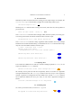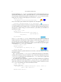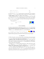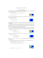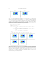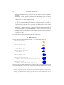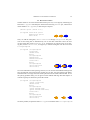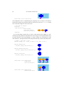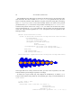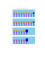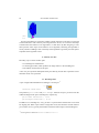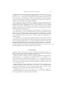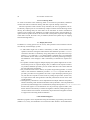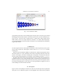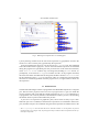
1
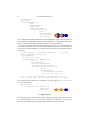
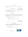
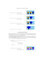
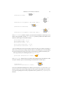
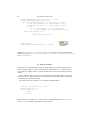
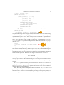
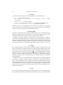
Under consideration for publication in J. Functional Programming
1
Slideshow: Functional Presentations
ROBERT BRUCE FINDLER
University of Chicago
(e-mail: [email protected])
MATTHEW FLATT
University of Utah
(e-mail: [email protected])
Abstract
Among slide-presentation systems, the dominant application offers essentially no abstraction capability. Slideshow, an extension of PLT Scheme, represents our effort over the last several years to
build an abstraction-friendly slide system. We show how functional programming is well suited to
the task of slide creation, we report on the programming abstractions that we have developed for
slides, and we describe our solutions to practical problems in rendering slides. We also describe experimental extensions to DrScheme that support a mixture of programmatic and WYSIWYG slide
creation.
1 Abstraction-Friendly Applications
Strand a computer scientist at an airport, and the poor soul would probably survive for
days with only a network-connected computer and five applications: an e-mail client, a
web browser, a general-purpose text editor, a typesetting system, and a slide-presentation
application. More specifically, while most any mail client or browser would satisfy the
stranded scientist, probably only Emacs or vi would do for editing, LATEX for typesetting,
and Microsoft PowerPointTM for preparing slides.
The typical business traveler would more likely insist on Microsoft WordTM for both
text editing and typesetting. Computer scientists may prefer Emacs and LATEX because
text editing has little to do with typesetting, and these different tasks are best handled by
different, specialized applications. More importantly, tools such as Emacs, vi, and LATEX
are programmable. Through the power of programming abstractions, a skilled user of these
tools becomes even more efficient and effective.
Shockingly, many computer scientists give up the power of abstraction when faced with
the task of preparing slides for a talk. PowerPoint is famously easy to learn and use, it
produces results that are aesthetically pleasing to most audience members, and it enables
users to produce generic slides in minutes. Like most GUI-/WYSIWYG-oriented applications, however, PowerPoint does not lend itself easily to extension and abstraction. PowerPoint provides certain pre-defined abstractions—the background, the default font and
color, etc.—but no ability to create new abstractions.
Among those who refuse to work without abstraction, many retreat to a web browser
(because HTML is easy to generate programmatically) or the various extension of TEX
2
R. B. Findler and M. Flatt
(plus a DVI/PostScript/PDF viewer). Usually, the results are not as aesthetically pleasing
as PowerPoint slides, and not as finely tuned to the problems of projecting images onto a
screen. Moreover, novice users of TEX-based systems tend to produce slides with far too
many words and far too few pictures, due to the text bias of their tool. Meanwhile, as a
programming language, TEX leaves much to be desired.
Slideshow, a part of the PLT Scheme application suite (PLT, n.d.), fills the gap left by
abstraction-poor slide presentation systems. First and foremost, Slideshow is an embedded DSL for picture generation, but it also provides direct support for step-wise animation, bullet-style text, slide navigation, image scaling (to fit different display and projector
types), cross-platform consistency (Windows, Mac OS, and Unix/X), and PostScript output
(for ease of distribution).
Functional programming naturally supports the definition of picture combinators, and
it enables slide creators to create new abstractions that meet their specific needs. Even
better, the Slideshow programming language supports a design recipe to help slide creators
build and maintain animation sequences. Our design recipe guides the programmer from a
storyboard sketch to an organized implementation, and it also suggests how changes in the
sketch translate into changes in the implementation.
Even with the best of programming languages, some slide sequences can benefit from a
dose of WYSIWYG construction. WYSIWYG tools should be part of the slide language’s
programming environment—analogous to GUI builders for desktop applications. We have
implemented extensions of the DrScheme programming environment that support interactive slide construction in combination with language-based abstraction.
Section 2 is a tour of Slideshow’s most useful constructs. Section 3 presents the Slideshow
design recipe for picture sequences. Section 4 explains Slideshow’s core implementation.
Section 5 briefly addresses practical issues for rendering slides on different media and
operating systems. Section 6 describes our prototype extension of DrScheme.
2 A Tour of Slideshow
A pict is the basic building block for pictures in Slideshow. Roughly, a pict consists of
a bounding box and a procedure for drawing relative to the box. Ultimately, a slide is
represented as a single pict to be drawn on the screen.
This section demonstrates how to use Slideshow primitives to generate slides like the
following, which might appear in a presentation about how fish gain weight when they eat
other fish.
Food Chain
Yikes!
7 lbs
10 lbs
Current total weight: 17 lbs
After big fish eats little one: 17 lbs
Slideshow: Functional Presentations
3
2.1 Pict Generators
Slideshow provides several functions for creating picts of simple shapes. For example, the
filled-rectangle function takes a height and a width and produces a pict:
(filled-rectangle 20 10)
Similarly, the text function takes a string, a font class, and a font size, and it produces a
pict for the text.
(text "10 lbs" ’(bold . swiss) 9)
10 lbs
The standard-fish function takes a height, width, direction symbol, color string, eyecolor string, and boolean to indicate whether the fish’s mouth is open:
(standard-fish 30 20 ’left "blue" "black" #t)
The standard-fish function’s many arguments make it flexible. If we need multiple
fish but do not need all of this flexibility, we can define our own fish function that accepts
only the color and whether the fish’s mouth is open:
;; fish : str[color] bool -> pict
(define (fish color open?)
(standard-fish 30 20 ’left color "black" open?))
(define big-fish (fish "blue" #f))
(define big-aaah-fish (fish "blue" #t))
2.2 Adjusting Picts
If we need fish of different sizes after all, instead of adding arguments to fish, we can
simply use Slideshow’s scale function:
(define little-fish (scale (fish "orange" #f) 0.7))
We certainly want to place our fish into an aquarium, which we can draw as a light-blue
rectangle behind the fish. The rectangle function does not accept a color argument;
instead, it generates a rectangle that uses the default color, and the colorize function
lets us adjust the default color for a pict. Thus, we can create a light-blue rectangle as
follows:
(colorize (filled-rectangle 20 10) "sky blue")
2.3 Combining Picts
To create a pict with two fish, we can use ht-append:
(ht-append 10 little-fish big-aaah-fish)
4
R. B. Findler and M. Flatt
The first argument to ht-append is an amount of space to put between the picts. It is
optional, and it defaults to 0. The ht part of the name ht-append indicates that the picts
are horizontally stacked and top-aligned. Analogously, the hb-append function bottomaligns picts. If, we want to center-align picts, we can use hc-append:
(define two-fish
(hc-append 10 little-fish big-aaah-fish))
Now we are ready to place the fish into an aquarium. Our old aquarium,
(colorize (filled-rectangle 20 10) "sky blue")
is not large enough to hold the two fish. We could choose a fixed size for the aquarium, but
if we later change the size constants in the fish function, then the aquarium might not be
the right size. A better strategy is to create a function aq that takes a pict and makes an
aquarium for the pict:
;; aq : pict -> pict
(define (aq p)
(colorize (filled-rectangle (pict-width p)
(pict-height p))
"sky blue"))
(aq two-fish)
The pict-width and pict-height functions take a pict and produce its width and
height, respectively. This aquarium is large enough to hold the fish, but it’s tight. We can
give the fish more room by adding space around two-fish with Slideshow’s inset
function, and then generate an aquarium pict. Finally, we put the fish and aquarium together
using Slideshow’s cc-superimpose function:
;; in-aq : pict -> pict
(define (in-aq p)
(cc-superimpose (aq (inset p 10)) p))
(in-aq two-fish)
The leftmost argument is placed bottommost in the stack, so the fish end up on top of the
aquarium rectangle.
The cc part of the name cc-superimpose indicates that the picts are centered horizontally and vertically as they are stacked on top of each other. Slideshow provides a
-superimpose function for each combination of l, c, or r (left, center, or right) with
t, c, or b (top, center, or bottom).
One additional mode of alignment is useful for text. When combining text of different
fonts into a single line of text, then neither ht-append nor hb-append produces the
right result in general, because different fonts have different shapes. Slideshow provides
hbl-append for stacking picts so that their baselines match.
;; lbs : num -> pict
(define (lbs amt)
(hbl-append (text (number->string amt) ’(bold . swiss) 9)
(text " lbs" ’swiss 8)))
(define 10lbs (lbs 10))
10 lbs
Slideshow: Functional Presentations
5
(define 7lbs (lbs 7))
7 lbs
(define 17lbs (lbs 17))
17 lbs
For multi-line text, hbl-append matches baselines for the bottommost lines. Slideshow
provides htl-append to make baselines match for topmost lines. Naturally, Slideshow
provides variants of -superimpose with tl and bl, as well.
Finally, Slideshow provides vl-append, vc-append, and vr-append to stack
picts vertically with left-, center-, and right-alignment. To add the labels to our aquarium
pict, we can use vl-append to first stack the aquarium on the “10 lbs” label, and then
use rbl-superimpose to add the “7 lbs” label to the bottom-right corner of the pict:
(define two-fish+sizes
(rbl-superimpose
(vl-append 5
(in-aq two-fish)
7lbs)
10lbs))
7 lbs
10 lbs
2.4 Picts and Identity
Pict objects are purely functional. A particular pict, such as little-fish can be used in
multiple independent contexts. Functions that adjust a pict, such as scale, do not change
the given pict, but instead generate a new pict based on the given one. For example, we can
combine two-fish and a scaled version of two-fish in a single pict:
(hc-append 10 two-fish (scale two-fish 0.5))
Picts nevertheless have an identity, in the sense of Scheme’s eq?, and each use of a
Slideshow function generates a pict object that is distinct from all other pict objects.
2.5 Finding Picts
To add an arrow from “7 lbs” to the little fish, we could insert an arrow pict into the
vl-append sequence (with negative space separating the stacked pict), but then adding
an arrow from “10 lbs” to the big fish would be more difficult.
Slideshow provides a more general way to extend a pict, which is based on finding the
relative location of sub-picts. To locate a sub-pict within an aggregate pict, Slideshow provides a family of operations beginning with find-. These operations rely on the identity
of picts to find one pict within another.
The suffix of a find- operation indicates which corner or edge of the sub-pict to find;
it is a combination of l, c, or r (left, center, or right) with t, tl, c, bl, or b (top, top
baseline, center, bottom baseline, or bottom). The results of a find- operation are the
coordinates of the found corner/edge relative to the aggregate pict.
A find- operation is often combined with place-over, which takes a pict, horizontal and vertical offsets, and a pict to place on top of the first pict. For example, we
can create a connecting arrow with arrow-line (which takes horizontal and vertical
displacements, plus the size of the arrowhead) and place it onto two-fish+sizes.
6
R. B. Findler and M. Flatt
(define-values (ax ay) (find-ct two-fish+sizes 7lbs))
(define-values (bx by) (find-cb two-fish+sizes little-fish))
(place-over two-fish+sizes
ax
(− (pict-height two-fish+sizes) ay)
(arrow-line (− bx ax) (− by ay) 6))
7 lbs
10 lbs
Since we need to multiple arrows, we abstract this pattern into a function:
;; connect : pict pict pict -> pict
(define (connect main from to)
(define-values (ax ay) (find-ct main from))
(define-values (bx by) (find-cb main to))
(place-over main
ax
(− (pict-height main) ay)
(arrow-line (− bx ax) (− by ay) 6)))
(define labeled-two-fish
(connect (connect two-fish+sizes
7lbs little-fish)
10lbs big-aaah-fish))
7 lbs
10 lbs
Slideshow provides a function that is like connect called add-arrow-line. In addition to the arguments of connect, add-arrow-line accepts the find- functions for
each sub-pict. Thus, connect can be implemented more simply as
;; connect : pict pict pict -> pict
(define (connect main from to)
(add-arrow-line 6 main from find-ct to find-cb))
Slideshow provides several libraries that are built in terms of finding picts. For example,
the "balloon.ss" library provides wrap-balloon for wrapping a pict into a cartoon
balloon, plus place-balloon for placing the balloon onto a pict.
(define yikes
(wrap-balloon (text "Yikes!" ’(bold . roman) 9)
’s 0 10)) ; spike direction and displacement
;; panic : pict -> pict
(define (panic p)
(place-balloon yikes p little-fish find-ct))
Yikes!
(panic two-fish)
The place-over operation preserves the bounding box of its first argument, instead
of extending it to include the placed pict. This behavior is useful for adding arrows and
balloons such that further compositions are unaffected by the addition. For example, we
can still put the fish into an aquarium after adding the panic balloon.
Yikes!
(in-aq (panic two-fish))
Slideshow: Functional Presentations
7
2.6 Ghosts and Laundry
We eventually want a slide sequence with variants of the aquarium pict. One variant should
have the little and big fish together in the aquarium, as before:
(define both-fish
(hc-append 10 little-fish big-fish))
(in-aq both-fish)
Another variant should have just the big fish—now even bigger, since it has eaten the little
fish. If we generate the pict as
(define bigger-fish
(scale big-fish 1.7))
(in-aq bigger-fish)
then our slides will not look right, because the aquarium changes shape from the first pict
to the second.
We can avoid this problem by constructing a large enough aquarium for the first pict.
Conceptually, we’d like to stack the large-fish pict on top of the pict with the two fish
together, and then put the combined pict in the aquarium (so that it is large enough to fit
both picts in both dimensions), and then hide the single fish.
The ghost function takes a picture and generates a picture with the same bounding box
as the given one, but with no drawing. Thus, we can create the right initial pict as follows:
(define all-fish-1
(in-aq (cc-superimpose
both-fish
(ghost bigger-fish))))
We can create the last slide by ghosting both-fish instead of bigger-fish:
(define all-fish-2
(in-aq (cc-superimpose
(ghost both-fish)
bigger-fish)))
Since both all-fish-1 and all-fish-2 contain all three fish, they are guaranteed to
be the same size.
If we try to add a label and arrow for the big fish, however, something goes wrong:
;; add-big-label : pict pict -> pict
(define (add-big-label all-fish wt)
(let ([labeled (vr-append 5 all-fish wt)])
(connect labeled wt big-fish)))
(add-big-label all-fish-1 10lbs)
10 lbs
8
R. B. Findler and M. Flatt
(add-big-label all-fish-2 17lbs)
17 lbs
The problem is that bigger-fish is a scaled version of big-fish, and even though
bigger-fish is ghosted in all-fish-1, it can still be found as a sub-pict. That
is, ghost makes big-fish invisible to the eye, but not to the find- operations. Thus,
big-fish exists twice in each all-fish- pict, and add-big-label finds the wrong
one in all-fish-1.
To hide a pict’s identity, Slideshow provides launder as a complement to ghost.
The launder function takes a pict and produces a pict with the same dimensions and
drawing, but without any findable sub-picts. To ensure that add-big-label finds the
right big-fish, we can both ghost and launder the pict to hide.
(define all-fish-1
(in-aq (cc-superimpose
both-fish
(launder (ghost bigger-fish)))))
(add-big-label all-fish-1 10lbs)
10 lbs
(define all-fish-2
(in-aq (cc-superimpose
(launder (ghost both-fish))
bigger-fish)))
(add-big-label all-fish-2 17lbs)
17 lbs
Alternately, we might define bigger-fish as (launder (scale big-fish 1.7)),
so that bigger-fish would never be confused with big-fish. In that case, we must
also adjust add-big-label to accept a target fish, either big-fish or bigger-fish.
2.7 From Pictures to Slides
Pict-construction primitives are only half of Slideshow’s library. The other half defines
pict operations that support common slide tasks and that cooperate with a slide-display
system. Common tasks include creating a slide with a title, creating text with a default
font, breaking lines of text, bulletizing lists, and staging bullet lines. Cooperating with
the display includes correlating titles with a slide-selection dialog and enabling clickable
elements within interactive slides.
Abstractly, a slide presentation is a sequence of picts. Thus, a presentation could be
represented as a list of picts, and a Slideshow program could be any program that generates such a list. We have opted instead for a more imperative design at the slide level: a
Slideshow program calls a slide function (or variants of slide) to register each individual slide’s content.1
1
We illustrate the effect of slide by showing a framed, scaled version of the resulting slide’s pict.
Slideshow: Functional Presentations
9
(slide
(scale big-fish 10))
We choose imperative registration through slide because a slide presentation is most easily written as a sequence of interleaved definitions and expressions, much like the examples
in section 2. A programmer could thread a list through the sequence, but threading is awkward to read and maintain. The picts that are registered for slides remain purely functional
(i.e., they cannot be mutated), so a small amount of imperative programming causes little
problem in practice. Furthermore, we usually write slide at the top-level, interspersed
with definitions, so each use of slide feels more declarative than imperative.
The slide/title function is similar to slide, except that it takes an extra string
argument. The string is used as the slide’s name, and it is also used to generate a title pict
that is placed above the supplied content picts. The title pict uses a standard (configurable)
font and is separated from the slide content by a standard amount.
Big Fish
(slide/title "Big Fish"
(scale big-fish 10))
The slide and slide/title functions do not merely register a slide. If they did, programmers would prefer to use more elaborate abstractions, and part of Slideshow’s job is to
provide the most useful of such abstractions. Thus, Slideshow allocates the relatively short
names slide, slide/title, etc. to functions that provide additional functionality.
The simplest such addition is that each slide function takes any number of picts, and it
concatenates them with vc-append using a separation of gap-size (which is 24). The
slide function then ct-superimposes the appended picts with a blank pict representing the screen (minus a small border). The slide/center function is like slide, except that it centers the slide content with respect to the screen. The slide/title/center
function accepts a title and also centers the slide.
Big Fish
Mmmm... fish
(slide/title/center "Big Fish"
(scale big-fish 10)
(text "Mmmm... fish" ’swiss 32))
10
R. B. Findler and M. Flatt
The set of pre-defined slide layouts includes only the layouts that we have found to be
most useful. Programmers can easily create other layouts by implementing functions that
call slide.
2.8 Managing Text
In the spirit of providing short names for particularly useful abstractions, Slideshow provides the function t for creating a text pict with a standard font and size (which defaults
to sans-serif, 32 units high). Thus, the label for the earlier example could have been implemented as (t "Mmmm... fish") instead of (text "Mmmm... fish" ’swiss
32). The bt function is similar to t, except that it makes the text bold, and it makes text
italic.
For typesetting an entire sentence, which might be too long to fit on a single line and
might require multiple fonts, Slideshow provides a para function. The para function
takes a width and a sequence of strings and picts, and it arranges the text and picts as a
paragraph that is bounded by the given width. In the process, para may break strings on
word boundaries. The width argument to para is often based on the client-w constant,
which is defined as the width of the entire slide minus a small margin.
Just One Fish
(slide/title/center "Just One Fish"
(scale big-fish 10)
(para (∗ 1/2 client-w)
"Give a man a fish, and"
"he’ll put it on a slide"))
Give a man a fish, and he'll put it
on a slide
The page-para function is like para, but with client-w as the implicit first width.
Slideshow accomodates bulleted lists with the item function. It is similar to para,
except that it adds a bullet to the left of the paragraph. In parallel to page-para and
para, the page-item function is like item, but with client-w built in.
Fish Story
(slide/title/center "Fish Story"
(page-item "One Fish")
(scale big-fish 6)
(page-item "Two Fish")
(scale (hc-append 10
little-fish
big-fish)
6))
One Fish
Two Fish
Note that, given a bullet pict, item is easily implemented in terms of para.
Slideshow: Functional Presentations
11
;; item : num pict ... -> pict
(define (item w . picts)
(htl-append (/ gap-size 2)
bullet
(apply para
(− w
(pict-width bullet)
(/ gap-size 2))
picts)))
Just as Slideshow provides many slide variants, it also provides many para and item
variants, including variants for right-justified or centered paragraphs and bulleted sub-lists.
The para∗ function, for example, typesets a paragraph like para, but it allows the result
to be more narrow than the given width (in case no individual line fills exactly the given
width).
2.9 Staging Slides
One way to stage a sequence of slides is to put one pict for each slide in a list, and then
map a slide-generating function over the list of picts:
;; aq-slide : pict -> void
(define (aq-slide all-fish)
(slide/title/center "Food Chain"
(scale all-fish 6)))
(map aq-slide (list all-fish-1 all-fish-2))
Food Chain
Food Chain
Interesting presentations usually build on this idea, and we discuss it more in section 3.
Much like text and hbl-append for typesetting paragraphs, however, this strategy
is awkward for merely staging bullets or lines of text on a slide. For example, when posing
a question to students, an answer may be revealed only after the students have a chance to
think about the question.
To support this simple kind of staging, the slide function (and each of its variants)
treats the symbol ’next specially when it appears in the argument sequence. All of the
picts before ’next are first used to generate a slide, and then the picts before ’next plus
the arguments after ’next are used to generate more slides.
(slide/title "Food Chain"
(scale all-fish-1 6)
(t "How many fish in the aquarium?")
’next
(bt "Two"))
12
R. B. Findler and M. Flatt
Food Chain
Food Chain
How many fish in the aquarium?
How many fish in the aquarium?
Two
The ’next symbol simplifies linear staging of slide content. The slide function also
supports tree-like staging of content through the ’alts symbol. The argument following
’alts must be a list of lists, instead of a single pict. Each of the lists is appended individually onto the preceding list of pict to generate a set of slides. The final list is further
appended with the remaining arguments (after the list of lists). The ’next and ’alts
symbols can be mixed freely to generate sub-steps and sub-trees.
(slide/title "Food Chain"
(scale all-fish-1 6)
’alts
(list (list (t "What if the big fish eats the little one?")
’next
(t "It will become 17 pounds"))
(list (t "What if the little fish eats the big one?")
’next
(t "It will become 17 pounds")))
’next
(t "But the little fish can’t eat the big one..."))
Food Chain
Food Chain
Food Chain
What if the big fish eats the little one?
What if the big fish eats the little one?
What if the little fish eats the big one?
It will become 17 pounds
Food Chain
What if the little fish eats the big one?
It will become 17 pounds
Food Chain
What if the little fish eats the big one?
It will become 17 pounds
But the little fish can't eat the big one...
With slide, page-item, ’next, ’alts, etc., a programmer can build a text-oriented
presentation in Slideshow almost as easily as in PowerPoint. The purpose of Slideshow,
however, is not to encourage bullet-point presentations, but to simplify the creation of more
interesting, graphical presentations—which is why we began with standard-fish instead of page-item. Having concluded a tour of Slideshow features, we now turn our
attention to the design of slide presentations.
Slideshow: Functional Presentations
13
3 How to Design Slide Presentations
The strength of functional programming is that it supports and encourages good program
design (Felleisen et al., 2001). We believe that Slideshow supports and encourages good
presentation design, not only because it is based on functional programming, but because
it directly supports a design recipe for image sequences.
This section demonstrates the design recipe for a single scene (i.e., a sequence of related
picts in a presentation). The example scene animates our earlier fish example to illustrate
conservation of mass in an aquarium: when one fish eats another, the total mass of the
aquarium content does not change.
The first step in designing any scene is to create a storyboard for the scene. A storyboard
sketches the sequence of individual frames, each of which corresponds to a slide. Our
example storyboard is shown in figure 1.
Fig. 1. Storyboard for the example talk
Once we have a storyboard, we must identify the main characters—that is, the elements
of the picture that define the overall layout across frames. We call the rest of the frame
elements the supporting cast; they will be layered on the basic frame as determined by the
main characters.
In this case, the fish are the main characters, because the layout of the fish determines
the overall shape of each frame in the sequence. In contrast, the water in the aquarium and
the weights and arrows are the supporting cast. We can draw the aquarium under the frame
shaped by the fish, and we can draw the arrows and weight labels on top.
The programming task is to convert a scene and the characters into expressions that
generate picts for the frames. There are four steps in our recipe:
1. Design an expression that produces the pict for each main character. A particular
character may change shape over multiple frames, so design one expression per view
of each character.
In this case, we have three characters, which are the three fish in the first frame. The
first two fish have only a single view each. The last fish has five: small with its mouth
open and closed, medium-sized with its mouth open and closed, and large with its
mouth closed.
2. Design a pict expression that includes all of the views of the main characters from
all frames in the scene. This pict may include a character in multiple places if the
character appears in different places in different frames. To generate a particular
14
R. B. Findler and M. Flatt
frame, we parameterize the pict expression to hide characters that do not appear in
the frame.
In this case, we must generate a pict that has the three fish in a line, plus different
views of the last fish on top of those fish. For example, the largest fish will be on top
of the first fish with their left edges touching.
3. Design pict expressions for the supporting cast. Unlike the main cast, each supporting cast pict should have the same dimensions as the entire frame, so it can be superimposed on its corresponding frame. Each supporting cast member is placed into
an appropriately sized blank pict at a position that is determined by the its location
in the complete frame.
In this case, we design overlays for the arrows and for the weights. Each weight will
be centered below its corresponding fish, and the arrows point from the top of the
weight to the bottom of the fish.
4. Design an expression that, for each frame, combines the main-character pict and the
supporting-cast picts.
Each of the following sections implements one step in the recipe.
3.1 Main Characters
Our main character expressions can re-use the fish function from section 2.
(define lunch-fish
(fish "orange" #f))
(define dinner-fish
(launder lunch-fish))
(define small-fish
(fish "blue" #f))
(define small-aaah-fish
(fish "blue" #t))
(define medium-fish
(launder (scale small-fish (sqrt 2))))
(define medium-aaah-fish
(launder (scale small-aaah-fish (sqrt 2))))
(define large-fish
(launder (scale small-fish (sqrt 3))))
In general, each of the main characters in our scene must have a separate identity from each
of the others and must not contain any of the others as sub-picts. Otherwise, the overlays
we build in step 3 might find the wrong main character.2
2
Technically, this particular scene does not need the the small, medium, or large fish to be laundered, but for
consistency we launder them anyway. The dinner fish, on the other hand, must be laundered or the scene will
look wrong. As you continue reading, see if you can guess how.
Slideshow: Functional Presentations
15
3.2 The Scene’s Frames
The first frame in our scene has three fish lined up in a row, so we begin by combining our
fish with hc-append. We add space between the fish using a blank pict, instead of an
initial number to hc-append, to make the space explicit.
(define spacer (blank 10 0))
(hc-append lunch-fish spacer
dinner-fish spacer
small-fish)
Next, we add the eating fish, small-aaah-fish through large-fish. The position of each eating fish is determined by one of the three initial fish. Since the nose
of each eating fish, such as medium-fish, should line of with the nose of an existing fish, such as lunch-fish, we might try to add the eating fish into the scene with
lc-superimpose.
(hc-append (lc-superimpose
large-fish
dinner-fish)
spacer
(lc-superimpose
medium-fish
medium-aaah-fish
lunch-fish)
spacer
(lc-superimpose
small-aaah-fish
small-fish))
On close examination of the spacing, however, we can see that the medium and large fish
have stretched the space between the original picts. In fact, the space between the dinner
and lunch fish is no longer the same as the space between the lunch and small fish. To see
the spacing problem clearly, we can ghost out the medium and large fish and compare it
with the original pict that shows just the first frame.
(hc-append (lc-superimpose
(ghost large-fish)
dinner-fish)
spacer
(lc-superimpose
(ghost medium-fish)
(ghost medium-aaah-fish)
lunch-fish)
spacer
(lc-superimpose
small-aaah-fish
small-fish))
To fix the problem, we push the calls to hc-append inside the calls to lc-superimpose.
16
R. B. Findler and M. Flatt
(lc-superimpose
large-fish
(hc-append dinner-fish
spacer
(lc-superimpose
medium-fish
medium-aaah-fish
(hc-append lunch-fish
spacer
(lc-superimpose
small-aaah-fish
small-fish)))))
Now, the large fish and the medium fish overlap with the fish to the right, but the storyboard
shows that the overlapping fish will never appear together in a single frame. Meanwhile,
this pict preserves the original spacing of the dinner, lunch, and small fish.
Once we have the basic layout designed, the design recipe tells us to parameterize it so
we can hide certain fish. In this case, we parameterize the scene with a list of the fish that
we want to show, and we define an on helper function to either show or hide each character
in the scene.
;; main-characters : (listof pict[main-char]) -> pict[frame]
(define (main-characters active)
(lc-superimpose
(on active large-fish)
(hc-append (on active dinner-fish)
spacer
(lc-superimpose
(on active medium-fish)
(on active medium-aaah-fish)
(hc-append (on active lunch-fish)
spacer
(lc-superimpose
(on active small-aaah-fish)
(on active small-fish)))))))
;; on : (listof pict[main-char]) pict[main-char] -> pict
(define (on set pict) (if (memq pict set) pict (ghost pict)))
To assemble the main characters for each frame, we simply apply main-characters
to a list of fish to show.
(define main1
(main-characters (list dinner-fish
lunch-fish
small-fish)))
3.3 Supporting Cast
For the supporting cast, we start with the fish’s weights. Typically, a supporting cast member’s position depends on one or more main characters. As it happens, we can go even
further for the weights by generating the label pict based on the area of a fish.
Slideshow: Functional Presentations
17
;; weight : pict[main-char] -> num
(define (weight fish)
(inexact->exact (round (∗ (pict-width fish)
(pict-height fish)
1/60))))
(define small-lbs (lbs (weight small-fish)))
10 lbs
To place the weight of the fish directly below the fish, we first compute the position of the
fish. Then, we can use place-over to combine a frame with the weight. The second
argument to place-over is the horizontal position of the left edge of the weight. The
following code ensures that the weight is centered below the fish. The third argument to
place-over is the vertical position, and the following code places the weight just below
the aquarium.
(define-values (fx fy) (find-cc main1 small-fish))
(define main1/weight
(place-over main1
(− fx
(/ (pict-width small-lbs)
2))
(+ (pict-height main1) 6)
small-lbs))
10 lbs
Combining the weight and the original scene in this manner helps us test our computation
of the weight’s coordinates, but the design recipe tells us to build an overlay pict that only
contains the weight. Building the overlay as a separate pict enables us to add or remove it
without disturbing the rest of the scene.
We can obtain a separate pict for the weight overlay by simply ghosting the input frame.3
;; weight-overlay : pict[frame] pict[main-char] pict[weight] -> pict
(define (weight-overlay frame fish weight)
(define-values (fx fy) (find-cc frame fish))
(place-over (ghost frame)
(− fx (/ (pict-width weight) 2))
(+ (pict-height frame) 6)
weight))
(add-bbox
(weight-overlay main1
small-fish
(lbs (weight small-fish))))
10 lbs
The other supporting cast members are the arrows. To draw an arrow from the small fish’s
weight to the small fish, we can use add-arrow-line.
(add-arrow-line 8
main1/weight
small-lbs find-ct
small-fish find-cb)
3
10 lbs
See the appendix for the implementation of add-bbox, which adds a gray box to the given pict. We use
add-bbox to show the location of the bounding box in a mostly blank image.
18
R. B. Findler and M. Flatt
Again, to satisfy the design recipe for this step, we must build a pict that draws only the
arrow.
(add-bbox
(add-arrow-line 8
(ghost main1/weight)
small-lbs find-ct
small-fish find-cb))
Once we have designed the arrow overlay for a single frame, we can abstract over its
construction, as with the weight overlay.
;; arrow-overlay : pict[frame] pict[main-char] pict[weight] -> pict
(define (arrow-overlay frame fish lbs)
(add-arrow-line 8
(ghost frame)
lbs find-ct
fish find-cb))
Now that we have defined the two overlays, we can write a single function that combines the them. Since place-over does not adjust the bounding box, the weight label is
placed below its input pict. So, when we combine the overlays, we must be careful to use
ct-superimpose.
;; overlay : pict[frame] pict[main-char] -> pict
(define (overlay pict fish)
(let∗ ([weight (lbs (weight fish))]
[w/weight (weight-overlay pict fish weight)])
(ct-superimpose
w/weight
(arrow-overlay w/weight fish weight))))
10 lbs
(add-bbox (overlay main1 small-fish))
3.4 Put It All Together
All that remains is to define a function that puts together the aquarium, the main characters
and the overlays, and then call the function once for each frame in the scene.
;; fish-scene : (listof pict[main-char]) -> pict
(define (fish-scene set)
(let ([frame (in-aq (main-characters set))])
(apply ct-superimpose
frame
(map (λ (fish) (overlay frame fish))
set))))
(fish-scene (list dinner-fish
lunch-fish
small-fish))
10 lbs
10 lbs
10 lbs
Slideshow: Functional Presentations
19
(fish-scene (list dinner-fish
lunch-fish
small-aaah-fish))
10 lbs
(fish-scene (list dinner-fish
medium-fish))
10 lbs
20 lbs
(fish-scene (list dinner-fish
medium-aaah-fish))
10 lbs
20 lbs
10 lbs
10 lbs
30 lbs
(fish-scene (list large-fish))
3.5 Exploiting the Design Recipe
By following the design recipe, we have established a clear connection between the scene’s
storyboard and its source code. If we imagine a change to the storyboard, the design recipe
helps us determine how to modify the implementation.
For example, suppose we decide to color the arrows that connect the weights to the
fish. The corresponding code is the the arrow-overlay function. Simply adding a
colorize expression to its body produces colored arrows.
(define (arrow-overlay frame fish lbs)
(colorize
(add-arrow-line 8
(ghost frame)
lbs find-ct
fish find-cb)
"purple"))
(fish-scene (list dinner-fish
lunch-fish
small-aaah-fish))
10 lbs
10 lbs
10 lbs
20
R. B. Findler and M. Flatt
(fish-scene (list large-fish))
30 lbs
This modification relies on implementing the supporting cast as overlays. If we had not
followed the design recipe and placed the arrow directly on the scene, colorize would
have colored the weights as well as the arrows.
;; Not what we wanted
(colorize
(add-arrow-line 8
main1/weight
small-lbs find-ct
small-fish find-cb)
"purple")
10 lbs
As a second change, suppose that we want to make the fish grow pudgier as it eats,
instead of growing equally in both dimensions. This change to the storyboard affects only
the main characters, and correspondingly, we need to modify only the definitions of the
main characters. The aquarium and arrows adapt automatically to the new fish dimensions.
;; pudgy : pict num -> pict
(define (pudgy p n) (scale p (expt n 1/4) (expt n 3/4)))
(define medium-fish
(launder (pudgy small-fish 2)))
(define medium-aaah-fish
(launder (pudgy small-aaah-fish 2)))
(define large-fish
(launder (pudgy small-fish 3)))
(fish-scene (list dinner-fish
lunch-fish
small-aaah-fish))
10 lbs
(fish-scene (list dinner-fish
medium-aaah-fish))
10 lbs
10 lbs
20 lbs
10 lbs
Slideshow: Functional Presentations
(fish-scene (list large-fish))
21
30 lbs
Finally, imagine generalizing from three fish to an arbitrary number of fish. Although
this change is more complex, the design recipe suggests a way to break down the changes
and points to a clear set of modifications to the code.
The first step is to adapt our definitions of the main characters. We can organize the them
into three lists: the fish that are eaten and the fish that do the eating, with their mouths both
open and closed.
(define fc 9)
(define meal-fish
(build-list (− fc 1)
(λ (i) (launder lunch-fish))))
(apply hc-append meal-fish)
(define eating-fish
(build-list fc
(λ (i) (launder (pudgy small-fish (+ i 1))))))
(apply hc-append eating-fish)
(define eating-aaah-fish
(build-list fc
(λ (i) (launder (pudgy small-aaah-fish (+ i 1))))))
(apply hc-append eating-aaah-fish)
22
R. B. Findler and M. Flatt
This modification also affects the second step of the design recipe: the placement of the
main characters. We must re-define main-characters to generalize from just three
fish to an arbitrary number of fish. With the exception of the first eating fish, each eating
fish is lc-superimposed on one of the food fish, and the rest of the scene is placed
just behind with spacer in between. The procedure in the body of main-characters
constructs this portion of the scene. Using foldl, we iterate over the three lists of fish.
The second argument to foldl is the initial pict, which contains only the first eating fish
in this case. The last three arguments of foldl correspond to lists of arguments to the
folding procedure.
(define (main-characters active)
(foldl (λ (meal-fish eating-fish eating-aaah-fish rest-of-scene)
(lc-superimpose
(on active eating-fish)
(on active eating-aaah-fish)
(hc-append (on active meal-fish)
spacer
rest-of-scene)))
(cc-superimpose (on active (car eating-fish))
(on active (car eating-aaah-fish)))
meal-fish
(cdr eating-fish)
(cdr eating-aaah-fish)))
(main-characters (append meal-fish eating-fish eating-aaah-fish))
The weight and arrow overlays remain the same, per fish, in the storyboard, so the code
from the third step of the design recipe does not change.
To follow the recipe’s fourth step and complete the modification, we define ith to
accept a frame number and produce the corresponding pict, using our earlier definition of
fish-scene.
;; ith : num -> pict
(define (ith i)
(fish-scene (cons (list-ref (if (even? i)
eating-fish
eating-aaah-fish)
(quotient i 2))
(sublist meal-fish (quotient i 2) (− fc 1)))))
Slideshow: Functional Presentations
23
(ith
0)
10 lbs
10 lbs
10 lbs
10 lbs
10 lbs
10 lbs
10 lbs
10 lbs
10 lbs
(ith
1)
10 lbs
10 lbs
10 lbs
10 lbs
10 lbs
10 lbs
10 lbs
10 lbs
10 lbs
(ith
6)
10 lbs
10 lbs
10 lbs
10 lbs
10 lbs
40 lbs
(ith
7)
10 lbs
10 lbs
10 lbs
10 lbs
10 lbs
40 lbs
24
R. B. Findler and M. Flatt
(ith
16)
90 lbs
Overall, generalizing to an arbitrary number of fish required us to abstract over the fish
construction and to write some list-processing functions. In fact, we can use this technique
to demonstrate the behavior of an algorithm in a slide show. By first designing a scene
that represents some aspect of the behavior of an algorithm, animating the algorithm is
merely a matter of adding a calls in the body of the algorithm to generate picts that capture
snapshots of the algorithm’s state.
4 Anatomy of a Pict
Internally, a pict consists of three parts:
• A bounding box and baselines.
• A drawing procedure, which produces an image relative to the bounding box.
• The identity and location of sub-picts.
A few core pict operations manipulate these parts directly, and all other operations can be
derived from the core operations.
4.1 Bounding Boxes
A pict’s height and width define a bounding box for the pict.4
height
(annotate lunch-fish)
width
The primitive pict-width and pict-height functions accept a pict and return the
width and height of the pict’s bounding box, respectively.
(pict-width lunch-fish) ; ⇒ 30
(pict-height lunch-fish) ; ⇒ 20
In addition to a bounding box, every pict has a top and bottom baseline that can be used
for aligning text. When a pict contains a single line of text, the baselines coincide. When a
pict contains no text, typically the baselines match the bottom edge of the bounding box.
4
See the appendix for definitions of annotate and annotate-all.
Slideshow: Functional Presentations
height
(annotate-all 10lbs)
10 lbs
25
bases
width
7 lbs
height
10 lbs
17 lbs
(annotate-all (vc-append 3 7lbs 10lbs 17lbs))
upper
base
width
lower
base
height
bases
(annotate-all lunch-fish)
width
upper
base
height
10 lbs
(annotate-all (vc-append 3 lunch-fish 10lbs))
width
lower
base
The pict-ascent primitive accepts a pict and returns the distance from the pict’s top
edge to the top baseline, and the pict-descent primitive produces the distance from
the pict’s bottom edge to the bottom baseline.
(pict-height 10lbs) ; ⇒ 11
(pict-ascent 10lbs) ; ⇒ 9
(pict-descent 10lbs) ; ⇒ 2
(pict-ascent lunch-fish) ; ⇒ 30
(pict-descent lunch-fish) ; ⇒ 0
A pict’s bounding box does not necessarily enclose all of the pict’s image, but usually it
does. In any case, the pict’s image is drawn relative to its bounding box, so the bounding
box and the baselines provide points relative to the image for alignment with other picts.
The only primitive pict-combining function is place-over.
(place-over lunch-fish 25 2 10lbs)
10 lbs
The place-over function does not combine the bounding boxes and baselines of the
two picts. Instead, it preserves the bounding box and baselines of the first pict.
10 lbs
height
(annotate-all
(place-over lunch-fish 25 2 10lbs))
bases
width
One way to enlarge the bounding box is to place a pict on top of a blank pict. The blank
function creates a pict with an empty image, and with a given width, height, ascent, and descent. We can package the necessary computations into a general dxdy-superimpose
function:
26
R. B. Findler and M. Flatt
;; dxdy-superimpose : pict num num pict -> pict
(define (dxdy-superimpose p dx dy q)
(let∗ ([w (max (pict-width p) (+ (pict-width q) dx))]
[h (max (pict-height p) (+ (pict-height q) dy))]
[a (min (pict-ascent p) (+ (pict-ascent q) dy))]
[d (min
(+ (− h (pict-height p)) (pict-descent p))
(+ (− h (pict-height q) dy) (pict-descent q)))])
(place-over (blank w h a d)
0 0
(place-over p dx dy q))))
height
(annotate-all
(dxdy-superimpose lunch-fish 25 2 10lbs))
10 lbs
width
upper
base
lower
base
Slideshow’s -append, -superimpose, and inset functions can all be implemented
similarly in terms of place-over, blank, pict-width, pict-height, pict-ascent,
and pict-descent.
4.2 Drawing Procedure
Most picts can be implemented in terms of simple shapes with stacking and placing operations. Simple shapes, in turn, are implemented with Slideshow’s dc primitive (where
“dc” stands for “drawing context”), which provides direct access to the underlying drawing
toolbox.
The dc function takes an arbitrary drawing procedure and a height, width, ascent, and
descent for the pict. When the pict is to be rendered, the drawing procedure is called with
a target drawing context and an offset.
For example, the four-argument blank function is implemented as
;; blank : num num num num -> pict
(define (blank w h a d)
(dc (λ (dest x y)
(void))
w h a d))
More usefully, we can define a hook function that is implemented using the draw-spline
and draw-line methods of a primitive drawing context.
Slideshow: Functional Presentations
27
;; hook : num num -> pict
(define (hook w h)
(dc (λ (dest x y)
(let ([mid-x (+ x (/ w 2))]
[mid-y (+ y (/ h 2))]
[far-x (+ x w)]
[far-y (+ y h)]
[d (/ w 3)])
(send dest draw-spline
x y x far-y mid-x far-y)
(send dest draw-spline
mid-x far-y far-x far-y far-x mid-y)
(send dest draw-line
far-x mid-y (− far-x d) (+ mid-y d))))
w h 0 h))
(define go-fish
(ht-append 5 (hook 5 12) lunch-fish))
The primitive drawing context is highly stateful, with attributes such as the current drawing
color and drawing scale. Not surprisingly, slides that are implemented by directly managing this state are prone to error, which is why we have constructed the pict abstraction.
Nevertheless, the state components show up in the pict abstraction in terms of attribute defaults, such as the drawing color or width of a drawn line. In particular, the linewidth,
colorize, and scale primitives change the line width, color, and scale of a pict produced by hook:
(scale
(colorize (linewidth 1 go-fish) "red")
2)
Although the underlying drawing context includes a current font as part of its state, a pict’s
font cannot be changed externally, unlike the pict’s scale, color, or line width. Changing a
pict’s font would mean changing the font of sub-picts, which would in turn would cause the
bounding box of each sub-pict to change in a complex way, thus invalidating computations
based on the sub-pict boxes. We discuss this design constraint further in section 5.2.
4.3 Sub-Picts
When a pict is created with place-over, the resulting pict stores the location of the
two input picts relative to the result bounding box. Since all pict-combination operators
are defined in terms of place-over, all combination operators reliably track sub-pict
locations.
The find-lt primitive searches a pict’s tree of sub-picts. All other find- variants are
easily implemented with find-lt, pict-width, pict-height, pict-ascent,
and pict-descent. The panorama primitive also searches a pict’s tree of sub-picts to
determine the enclosing bounding box.
Finally, three other primitives manipulate sub-pict information. The ghost and launder
primitives provide independent control of a pict’s image and sub-pict records. The scale
function, which is primitive is terms of adjusting pict images, also explicitly manages the
effect of scaling on sub-picts locations.
28
R. B. Findler and M. Flatt
4.4 Primitives
To summarize, the following are the essential primitives for Slideshow picts:
• dc — the main constructor of picts.
• pict-width, pict-width, pict-descent, and pict-ascent — dimension accessors.
• place-over — combination operator.
• find-lt, launder, ghost, panorama — operations to manage sub-picts.
• scale, linewidth, and colorize — image-adjusting operations.
All other operations can be implemented in terms of the above operations. For historical
reasons, the primitives in the implementation are less tidy than this set, but Slideshow
continues to evolve toward a more principled implementation.
5 Rendering Slides
Slideshow is implemented as a PLT Scheme application (PLT, n.d.). PLT Scheme provides
the primitive drawing contexts accessed by dc, as well as the widget toolbox for implementing the Slideshow presentation window and other interface elements.
Slideshow is designed to produce consistent results with any projector resolution, as
well as when generating PostScript versions of slides. The main challenges for consistency
concern pict scaling and font selection, as discussed in the following sections. We also
comment on Slideshow’s ability to condense staged slides for printing, to pre-render slides
to minimize delays during a presentation, and to trigger interactions during a presentation.
5.1 Scaling
Since 1024x768 displays are most common, Slideshow defines a single slide to be a pict
that is 1024x768 units. The default border leaves a 984x728 region for slide content. These
units do not necessarily correspond to pixels, however. Depending on the display at presen25
tation time, the pict is scaled (e.g., by a factor of 32
for an 800x600 display). If the display
aspect is not 4:3, then scaling is limited by either the display’s width or height to preserve
the pict’s original 4:3 aspect ratio, and unused screen space is painted black. Typically,
unused space appears when viewing slides directly on a desktop machine, such as during
slide development.
Slideshow does not use a special file format for slide presentations. Instead, a Slideshow
presentation is a program, and pict layouts are computed every time the presentation is
started. (This computation is rarely so expensive that it inteferes with interactive development.) Consequently, the target screen resolution is known at the time when slides are built.
This information can be used, for example, to scale bitmap images to match the display’s
pixels, instead of units in the virtual 1024x768 space. Information about the display is also
useful for font selection.
5.2 Fonts
Fonts are not consistently available across operating systems, or even consistently named.
To avoid platform dependencies, Slideshow presentations typically rely on PLT Scheme’s
Slideshow: Functional Presentations
29
mapping of platform-specific fonts through portable “family” symbols, such as ’roman
(a serif font), ’swiss (a sans-serif font, usually Helvetica), ’modern (a fixed-width
font), and ’symbol (a font with Greek characters and other symbols). PLT Scheme users
control the family-to-font mapping, so a Slideshow programmer can assume that the user
has selected reasonable fonts. Alternately, a programmer can always name a specific font,
though at the risk of making the presentation unportable.
Since specific fonts vary across platforms, displays, and users, the specific layout of
picts in a Slideshow presentation can vary, due to different bounding boxes for text picts.
Nevertheless, as long as a programmer uses pict-width and pict-height instead
of hard-wiring text sizes, slides display correctly despite font variations. This portability
depends on computing pict layouts at display time, instead of computing layouts in advance
and distributing pre-constructed picts.
Text scaling leads to additional challenges. For many displays, a font effectively exists
only at certain sizes; if a pict is scaled such that its actual font size would fall between
existing sizes, the underlying display engine must substitute a slightly larger or smaller
font. Consequently, a simple scaling of the bounding box (in the 1024x768 space) does
not accurately reflect the size of the text as it is drawn, leading to overlapping text or
unattractive gaps.
To compensate for text-scaling problems, Slideshow determines the expected scaling of
slides (based on the current display size) before generating picts. It then uses the expected
scale to generate a bounding box for text picts that will be accurate after scaling. Occasionally, the predicted scale is incorrect because the programmer uses the scale operation
in addition to the implicit scale for the target display, but this problem is rare. When necessary, the programmer can correct the scale prediction by using the scale/improve-new-text
form and creating text picts within the dynamic extent of this form.
5.3 Printing Slides
A drawing context in PLT Scheme is either a bitmap display (possibly offscreen) or a
PostScript stream. Thus, printing a Slideshow presentation is as simple as rendering the
slides to a PostScript drawing context instead of a bitmap context.
Slideshow provides a “condense” mode for collapsing staged slides. Collapse mode automatically ignores ’next annotations; a programmer can use ’next! instead of ’next
to force separate slides in condense mode. In contrast, ’alts annotations cannot be ignored, because each alternative can show different information. A Slideshow programmer
can indicate that intermediate alternatives should be skipped in condense mode by using
’alts˜ instead of ’alts.
Slideshow synchronizes page numbering in condensed slides with slide numbering in
a normal presentation. In other words, when slide skips a ’next annotation, it also
increments the slide number. As a result, a condense slide’s number is actually a range,
indicating the range of normal slides covered by the condensed slide.
Programmers can use the condense? and printing? predicates to further customize slide rendering for condense mode and printing. A skip-slides! function allows the programmer to increment the slide count directly.
30
R. B. Findler and M. Flatt
5.4 Pre-rendering Slides
To avoid screen flicker when advancing slides in an interactive presentation, Slideshow
renders each slide in an offscreen bitmap, and then copies the bitmap to the screen.
The time required to render a slide is rarely noticeable, but since a programmer can create arbitrary complex picts or write arbitrarily complex code that uses the drawing context
directly, the rendering delay for some slides can be noticeable. To ensure instantaneous
response in the common case, Slideshow pre-renders the next slide in the presentation sequence while the speaker dwells on the current slide. (If the speaker requests a slide change
within half a second, the slide is not pre-rendered, because the speaker may be stepping
backward through slides.)
5.5 Display Interaction
In addition to creating pictures for the screen, slide presenters must sometimes interact
more directly with the display system:
• A slide author might wish to attach a commentary to slides, for the benefit of the
speaker or for those viewing the slides after the talk. Slideshow provides a comment
constructor that takes a commentary string and produces an object that can be supplied to slide. When the slide function finds a comment object, it accumulates
the comment into the slide’s overall commentary (instead of generating an image).
The Slideshow viewer displays a slide’s commentary on demand in a separate window.
• If a speaker’s machine supports multiple displays, the speaker might like to see comments and a preview on a private display. Thus, in addition to the separate commentary window, Slideshow provides a preview window that shows the current slide and
the next slide in the presentation.
• For presentations that involve demos, the speaker might like hyperlinks on certain
slides to start the demos. Slideshow provides a clickback operator that takes a
pict and a procedure of no arguments; the result is a pict that displays like the given
one, but that also responds to mouse clicks by calling the procedure. (In this case,
we exploit the fact that slide generation and slide presentation execute on the same
virtual machine.)
• Although many “animations” can be implemented as multiple slides that the speaker
advances manually, other animations should be entirely automatic. Currently, Slideshow
provides only minimal support for such animations, though an imperative scroll-transition
function that registers a scroll animation over the previously registered slide. (This
feature has been used mainly to animate an algebraic reduction, making the expression movements easier to follow.) In the future, the pict abstraction might be enriched
to support more interesting kinds of animation.
6 Environment Support
Slideshow programs can be implemented using the DrScheme programming environment
(Findler et al., 1997), since Slideshow is an extension of PLT Scheme. All of DrScheme’s
Slideshow: Functional Presentations
31
Fig. 2. Picts in DrScheme’s REPL
programming tools work as usual, including the on-the-fly syntax colorer, the syntax checker,
the debugger, and the static analyzer. Non-textual syntax can be used in a Slideshow program, such as a test-case boxes, comment boxes, or XML boxes (which support literal
XML without concern for escape characters) (Clements et al., 2004). More importantly,
we can use DrScheme’s extension interface to add new tools to DrScheme that specifically
support slide creation.
6.1 REPL Picts
To better support interactive development, DrScheme’s read-eval-print-loop (REPL) prints
picts as they are drawn in a slide. Figure 2 shows a call to main-characters and the
resulting pict.
Each pict result in DrScheme’s REPL is itself interactive. When the programmer moves
the mouse pointer over a pict, DrScheme shows sub-pict bounding boxes that enclose the
pointer. In the figure, the narrow bounding box corresponds to the blue fish under the
pointer, and the wide bounding box corresponds to an intermediate pict from hc-append.
By default, DrScheme does not show bounding boxes that contain other bounding boxes
around the pointer (so the visible bounding boxes are minimal), but pressing the Alt (or
Meta) key exposes all of the bounding boxes that enclose the pointer. Pressing the Control
key shows all bounding boxes in the entire pict. Pressing the Shift key toggles the color of
each bounding box between black and white.
6.2 Tracing Picts
Figure 3 shows a screen dump for another tool. This tool records all picts that are generated
during the run of a Slideshow program. It then highlights each expression that produced
32
R. B. Findler and M. Flatt
Fig. 3. Mousing over expressions to see resulting picts
a pict by drawing a black box at the start of the expression. A programmer can move the
mouse over a box to see the pict(s) generated by the expression.5
In the screen dump, the mouse is over the start of an hc-append call. The right-hand
side of the window shows eight picts—one for each time that the expression was evaluated
during the program run. Specifically, the first pict shows the result of the first evaluation,
where rest-of-scene contains only one eating fish (including its aaah variant, superimposed), so the result of hc-append contains two fish. As the program continued,
this result was further extended with an eating fish, and then it became rest-of-scene
for the evaluation of the hc-append expression, and so on. Overall, the expression under
the mouse is evaluated eight times when the program is run, so eight results are shown for
the expression.
6.3 WYSIWYG Picts
The left-hand side of figure 4 shows a program that uses WYSIWYG layout for a composite
pict. The box with a projector-screen icon in its top-right corner is a pict box. Inside the
pict box, each box with a top-right the comma (suggestive of unquote) is a Scheme box.
A programmer can create any number of Scheme boxes within a pict box, and then drag
the Scheme boxes to position them within the pict box.
A pict box is an expression in graphical syntax, and its result is always a pict value.
When the pict box is evaluated, its Scheme-box expressions are evaluated to obtain subpicts, and these sub-picts are combined using the relative positions of Scheme boxes in the
5
The lc-superimpose call in the third line has no black box because it is in tail position. To preserve
tail-calls (Steele, 1977; Clinger, 1998), our prototype tool only records the values of expressions that are syntactically in tail position.
Slideshow: Functional Presentations
33
Fig. 4. A pict box containing Scheme boxes
source pict box. In this example, the program defines freeform-swimmers as a pict
that contains a school of manually positioned fish.
The right-hand side of figure 4 shows the same program, but after the programmer has
toggled the box to preview mode. In preview mode, each Scheme box is replaced with
the image of the pict that resulted from the most recent evaluation of the Scheme box.
(Preview mode is not available until after the program has been run once.) In this way,
a programmer can arrange the content of a pict box using actual images, instead of just
Scheme expressions.
Pict boxes illustrate how a programming environment can provide WYSIWYG tools
that complement the language’s abstraction capabilities. A pict box can be placed in any
expression position, and Scheme boxes are lexically scoped within the pict-box expression.
For example, a pict box can be placed into a function, and then a Scheme box within the
pict box can access arguments of the function. In this way, a programmer can use both
WYSIWYG editing and programmatic construction of picts, instead choosing one or the
other.
7 Slideshow Design and Related Work
By far, the most closely related work to Slideshow is Slithy (Zongker, 2003), which is a
Python-based tool for building slide presentations. Slithy is designed specifically to support movie-like animation, whereas Slideshow mainly supports slide-stepping animation.
Like Slideshow, however, Slithy provides a programmatic interface for slide construction,
manages the display of slides directly, and supports an explicit set of design principles
for presentation authors. Slithy’s slide-construction combinators seem more primitive than
Slideshow’s; most of the work to implement a Slithy presentation is in building animations
directly, much like building pictures with Slideshow’s dc primitive. A pict-like layer of
abstraction would support our design recipe in Slithy, but more work is required to adapt
the pict abstraction to fully support movie animation. The Slithy authors have identified
principles for slide animation (Zongker & Salesin, 2003) that should guide the design of
new animation abstractions.
Slideshow’s pict abstraction is by no means the first language designed for generating
pictures, and Slideshow’s picture constructors are similar to those of Henderson’s func-
34
R. B. Findler and M. Flatt
tional pictures (Henderson, 1982), MLgraph (Chailloux et al., 1997), Pictures (Finne &
Peyton Jones, 1995), Functional PostScript (Shivers & Sae-Tan, 2004), FPIC (Kamin &
Hyatt, 1997), pic (Kernighan, 1991), MetaPost (Hobby, 1992), and many other systems.
Unlike pic and MetaPost (but like MLgraph, etc.), Slideshow builds on a general-purpose
programming language, so it can support modular development, it allows programmers to
write maintainable code, libraries, and tests, and it is supported by a programming environment. MLgraph, Pictures, Functional PostScript, and FPIC provide a richer set of transformation operations (mainly because they all build on PostScript), while Slideshow provides
a richer set of text-formatting operations. More fundamentally, Slideshow’s combination
of find-, ghost, and launder appears to be unique. These operations reflect generally the way that Slideshow is tailored for slide creation, and specifically how Slideshow
supports a design recipe for slide sequences.
In the IDEAL (Van Wyk, 1981) picture language, programmers define pictures by describing constraints, such as “arrow X’s endpoint is attached to box Y’s right edge.” In
Slideshow, the programmer effectively writes a constraint solver manually, using functions
like pict-width ands find-lt. We have opted for the more direct functional style,
instead of a constraint-based language, because we find that many patterns of constraints
are easily covered by basic combinators (such as vl-append), while other patterns of
constraints (like adding lines to connect nodes) are easily abstracted into new functions.
Our choice of direct computation, instead of using constraints, affects the kinds of properties that can be adjusted from outside a pict. As discussed in section 5.2, a pict’s font
cannot be changed externally, because changing the font would invalidate computations
based on the pict’s bounding box. In a constraint-based system, or where all primitive pictcombination operations are encapsulated in operations like vc-append, then invalidated
computations can be re-executed. With more general combinations using place-over,
however, the offsets are computed by arbitrary Scheme code, so that automatic re-calculation
is not generally possible. Functional reactive programming (Elliott & Hudak, 1997) might
be the right solution to this problem, and we hope to explore this possibility. Meanwhile,
Slideshow’s current trade-off (flexible place-over versus inflexible fonts) has worked
well in practice. If a pict needs to be parameterized by its font, we simply use functional
abstraction or parameterize.
Countless packages exist for describing slides with an HTML-like notation. Such packages typically concentrate on arranging text, and pictures are imported from other sources.
Countless additional packages exists for creating slides with LATEX, including foiltex and
Prosper (Van Zandt, n.d.). With these packages, LATEX remains well adapted for presenting
math formulae and blocks of text, but not for constructing pictures, and not for implementing and maintaining abstractions.
Like Slideshow, Skribe (Seranno & Gallesio, n.d.; Seranno & Gallesio, 2002) builds on
Scheme to support programmatic document creation in a general-purpose functional language. Skribe’s architecture targets mainly the creation of articles, books, and web pages.
Since Skribe includes a LATEX-output engine, appropriate bindings could added to Skribe
to create slides through LATEX-based packages.
Unlike Slideshow, most slide-presentation systems (including all LATEX-based, PostScriptbased, and PDF-based systems) treat the slide viewer as an external tool. Separating the
viewer from the slide-generation language makes display-specific customization more dif-
Slideshow: Functional Presentations
35
ficult, and it inhibits the sort of integration with a programming environment that we advocate. An integrated viewer, meanwhile, can easily support executable code that is embedded within slides. Embedded code is particularly useful in a presentation about programming or about a software system, since an “eval” hyperlink can be inserted into any
slide. More generally, Slideshow gives the presentation creator access to the complete PLT
Scheme GUI toolbox, so anything is possible.
8 Conclusion
In only the last few years, laptop-projected slides have become the standard vehicle for
delivering talks, and tools other than PowerPoint are still catching up. We offer Slideshow
as a remedy to PowerPoint’s lack of abstraction, HTML’s lack of flexibility, and LATEX’s
lack of maintainability. We also offer a design recipe for slide sequences that is supported
by Slideshow’s set of primitives.
Programmatic construction of pictures and slides is probably not for everyone, even with
powerful programming-environment tools. For various reasons, many people will prefer to
create pictures and slides in PowerPoint and without significant abstraction, no matter how
nice the language of picture construction.
For the authors’ tastes and purposes, however, programmatic construction works well,
and we believe that it appeals to many programmers. In our slides, with proper code abstraction, we can quickly experiment with different configurations of a picture, add slideby-slide animation, and evolve ever more general libraries to use in constructing talks.
Many tasks can be automated entirely, such as typesetting code and animating reduction
sequences.
All of the figures in this paper are generated by Slideshow’s pict library, using exactly
the code as shown.6 In fact, like many other picture languages, Slideshow began as a system for generating figures for papers, and the core pict language works equally well on
paper and on slides. A picture language alone is not enough, however; most of our effort behind Slideshow was in finding appropriate constructs for describing, staging, and
rendering slides.
For further information on using Slideshow and for sample slide sets—including slides
for conference talks and two courses—see the following web page:
http://www.plt-scheme.org/software/slideshow/
6
We used Slideshow version 299.24, and we re-defined the slide operations to produce boxed picts.
36
R. B. Findler and M. Flatt
Appendix: Annotate implementation
;; add-bbox : pict -> pict
(define (add-bbox p) (apply-colorized add-bbox∗ p))
;; annotate : pict -> pict
(define (annotate p) (apply-colorized annotate∗ p))
;; annotate-all : pict -> pict
(define (annotate-all p) (apply-colorized annotate-all∗ p))
;; Non-colorized versions
;; add-bbox* : pict -> pict
(define (add-bbox∗ p)
(refocus (cc-superimpose p (rectangle (pict-width p)
(pict-height p)))
p))
;; annotate* : pict -> pict
(define (annotate∗ p) (add-bbox-labels (add-bbox∗ p)))
;; annotate-all* : pict -> pict
(define (annotate-all∗ p) (add-baselines (annotate∗ p)))
;; apply-colorized : (pict -> pict) pict -> pict
;; colorizes the annotations of ‘annote’
(define (apply-colorized annote p)
(cc-superimpose
p
(colorize (annote (ghost p)) bbox-color)))
;; add-bbox-labels : pict -> pict
;; Add "height" and "width" bars and labels, but
;; don’t change the boundbing box
(define (add-bbox-labels p)
(refocus (vr-append
bbox-sep
(hc-append bbox-sep
(hc-append (label "height")
(vc-append
(hline 5 0)
(vline 0 (pict-height p))
(hline 5 0)))
p)
(vc-append (hc-append (vline 0 5)
(hline (pict-width p) 0)
(vline 0 5))
(label "width")))
p))
;; add-baseline-lines : pict -> pict
;; Add baseline lines within the bbox
(define (add-baseline-lines p)
(let ([hl (hline (pict-width p) 0)])
(place-over (place-over p
0 (− (pict-height p) (pict-descent p))
hl)
Slideshow: Functional Presentations
0 (pict-ascent p)
hl)))
;; add-baselines : pict -> pict
;; Add baseline labels and arrows
(define (add-baselines p)
(let ([p (add-baseline-lines p)])
(if (practically= (pict-descent p)
(− (pict-height p) (pict-ascent p)))
;; Show baselines together
(add-baseline p
(pict-descent p)
(label "bases")
hc-append)
;; Show baselines separately
(add-baseline (add-baseline p
(pict-descent p)
(label "lower" "base")
ht-append)
(− (pict-height p) (pict-ascent p))
(label "upper" "base")
hb-append))))
;; add-baseline : pict num pict (num pict pict -> pict) -> pict
;; Add one baseline, dy from top of p; combine given
;; label with arrow using xx-append; don’t change
;; the bounding box
(define (add-baseline p dy lbl xx-append)
(place-over
p
(+ (pict-width p) bbox-sep)
(− (pict-height p) dy)
(refocus (xx-append 2 little-arrow lbl) little-arrow)))
;; label : str ... -> pict
;; Build a label
(define (label . strs)
(apply vl-append −2 (map (λ (str)
(text str ’swiss 8))
strs)))
;; practically= : num num -> bool
(define (practically= a b)
(let ([epsilon 0.01])
(and (< (− a epsilon) b)
(> (+ a epsilon) b))))
;; Constants
(define bbox-sep 5)
(define bbox-color "gray")
(define little-arrow
(inset (arrow-line (∗ −2 bbox-sep) 0 bbox-sep)
(∗ 2 bbox-sep) 0 0 0))
37
38
R. B. Findler and M. Flatt
References
Chailloux, Emmanuel, Cousineau, Guy, & Suárez, Ascánder. (1997). The MLgraph system.
Clements, John, Felleisen, Matthias, Findler, Robert Bruce, Flatt, Matthew, & Krishnamurthi, Shriram. (2004). Fostering little languages. Dr. Dobb’s journal, Mar., 16–24.
Clinger, William D. (1998). Proper tail recursion and space efficiency. Pages 174–185 of: Proc.
ACM conference on programming language design and implementation.
Elliott, Conal, & Hudak, Paul. (1997). Functional reactive animation. Pages 263–273 of: Proc. ACM
international conference on functional programming.
Felleisen, Matthias, Findler, Robert Bruce, Flatt, Matthew, & Krishnamurthi, Shriram. (2001). How
to design programs. Cambridge, Massachusetts: The MIT Press. http://www.htdp.org/.
Findler, Robert Bruce, Flanagan, Cormac, Flatt, Matthew, Krishnamurthi, Shriram, & Felleisen,
Matthias. 1997 (Sept.). DrScheme: A pedagogic programming environment for Scheme. Pages
369–388 of: Proc. international symposium on programming languages: Implementations, logics,
and programs.
Finne, Sigbjorn, & Peyton Jones, Simon. 1995 (July). Pictures: A simple structured graphics model.
Proc. Glasgow functional programming workshop.
Henderson, Peter. (1982). Functional geometry. Pages 179–187 of: Proc. ACM conference on Lisp
and functional programming.
Hobby, John D. (1992). A user’s manual for MetaPost. Computer science technical report. AT&T
Bell Laboratories. CSTR-162.
Kamin, Samual N., & Hyatt, David. 1997 (Oct.). A special-purpose language for picture-drawing.
Pages 297–310 of: Proc. USENIX conference on domain-specific languages.
Kernighan, Brian W. (1991). PIC — a graphics language for typesetting, user manual. Computer
science technical report. AT&T Bell Laboratories. CSTR-116.
PLT. PLT Scheme. www.plt-scheme.org.
Seranno,
Manuel,
&
Gallesio,
Erick.
Skribe
home
page.
http://www.inria.fr/mimosa/fp/Skribe.
Seranno, Manuel, & Gallesio, Erick. 2002 (Oct.). This is Scribe! Pages 31–40 of: Proc. workshop
on Scheme and functional programming.
Shivers, Olin, & Sae-Tan, Wendy. (2004). Functional PostScript: Industrial-strength 2D functional
imaging. In preparation. http://www.scsh.net/resources/fps.html.
Steele, Guy Lewis. (1977). Debunking the “expensive procedure call” myth, or procedure call implementations considered harmful, or LAMBDA, the ultimate GOTO. Pages 153–162 of: Proc.
ACM conference.
Van Wyk, Christopher J. (1981). IDEAL user’s manual. Computer science technical report. AT&T
Bell Laboratories. CSTR-103.
Van Zandt, Timothy. Prosper. prosper.sourceforge.net.
Zongker, Douglas. (2003). Creating animatation for presentations. Ph.D. thesis, University of Washington.
Zongker, Douglas, & Salesin, David. (2003). On creating animated presentations. Eurographics/SIGGRAPH symposium on computer animation.