Download Slideshow: Functional Presentations

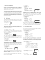
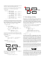
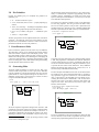
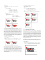
Slideshow: Functional Presentations
Robert Bruce Findler
Matthew Flatt
University of Chicago
University of Utah
[email protected]
[email protected]
Abstract
Among slide-presentation systems, the dominant application offers
essentially no abstraction capability. Slideshow, an extension of
PLT Scheme, represents our effort over the last several years to
build an abstraction-friendly slide system. We show how functional
programming is well suited to the task of slide creation, we report on the programming abstractions that we have developed for
slides, and we describe our solutions to practical problems in rendering slides. We also describe a prototype extension to DrScheme
that supports a mixture of programmatic and WYSIWYG slide creation.
Categories and Subject Descriptors
H.4.1 [Information Systems Applications]: Office Automation;
I.7.2 [Document and Text Processing]: Document Preparation
General Terms
Languages
1
Abstraction-Friendly Applications
Strand a computer scientist at an airport, and the poor soul would
probably survive for days with only a network-connected computer
and five applications: an e-mail client, a web browser, a generalpurpose text editor, a typesetting system, and a slide-presentation
application. More specifically, while most any mail client or
browser would satisfy the stranded scientist, probably only Emacs
or vi would do for editing, LATEX for typesetting, and Microsoft
PowerPointTM for preparing slides.
The typical business traveler would more likely insist on Microsoft
WordTM for both text editing and typesetting. In part, computer
scientists may prefer Emacs and LATEX because text editing has little
to do with typesetting, and these different tasks are best handled by
different, specialized applications. More importantly, tools such
as Emacs, vi, and LATEX are programmable. Through the power
Permission to make digital or hard copies of all or part of this work for personal or
classroom use is granted without fee provided that copies are not made or distributed
for profit or commercial advantage and that copies bear this notice and the full citation
on the first page. To copy otherwise, to republish, to post on servers or to redistribute
to lists, requires prior specific permission and/or a fee.
ICFP’04, September 19–21, 2004, Snowbird, Utah, USA.
Copyright 2004 ACM 1-58113-905-5/04/0009 ...$5.00
of programming abstractions, a skilled user of these tools becomes
even more efficient and effective.
Shockingly, many computer scientists give up the power of abstraction when faced with the task of preparing slides for a talk.
PowerPoint is famously easy to learn and use, it produces results
that are aesthetically pleasing to most audience members, and it
enables users to produce generic slides in minutes. Like most GUI/WYSIWYG-oriented applications, however, PowerPoint does not
lend itself easily to extension and abstraction. PowerPoint provides
certain pre-defined abstractions—the background, the default font
and color, etc.—but no ability to create new abstractions.
Among those who refuse to work without abstraction, many retreat
to a web browser (because HTML is easy to generate programmatically) or the various extension of TEX (plus a DVI/PostScript/PDF
viewer). Usually, the results are not as aesthetically pleasing as
PowerPoint slides, and not as finely tuned to the problems of projecting images onto a screen. Moreover, novice users of TEX-based
systems tend to produce slides with far too many words and far too
few pictures, due to the text bias of their tool. Meanwhile, as a
programming language, TEX leaves much to be desired.
Slideshow, a part of the PLT Scheme application suite [10], fills the
gap left by abstraction-poor slide presentation systems. First and
foremost, Slideshow is an embedded DSL for picture generation,
but it also provides direct support for step-wise animation, bulletstyle text, slide navigation, image scaling (to fit different display
and projector types), cross-platform consistency (Windows, Mac
OS, and Unix/X), and PostScript output (for ease of distribution).
Functional programming naturally supports the definition of picture
combinators, and it enables slide creators to create new abstractions
that meet their specific needs.
In this paper, we mainly demonstrate how Slideshow as a programming language supports abstraction, but slide creators can also
benefit from a measured dose of WYSIWYG slide construction.
WYSIWYG tools should be part of the slide language’s programming environment, analogous to GUI builders for desktop applications. We therefore report on experimental extensions of the
DrScheme programming environment that support interactive slide
construction along with language-based abstraction.
Section 2 describes Slideshow’s primitives for picture generation,
and Section 3 shows how we build on these operations to address common slide-construction tasks. Section 4 briefly addresses
practical issues for rendering slides on different media and operating systems. Section 5 describes our prototype extension of
DrScheme.
2
Picture Combinators
A pict is the basic building block for pictures in Slideshow.
Roughly, a pict consists of a bounding box and a procedure for
drawing relative to the box. Ultimately, a slide is represented as a
single pict to be drawn on the screen.
As a running example, suppose that we wish to illustrate graph
searching to novice programmers, showing how a graph of people
is traversed to find the name of a person who lives in a particular
city. The illustration will contain boxes labeled with names and locations, directed connections among the boxes, an arrow indicating
the starting box, and a cloud that stands in place of many unspecified boxes and connections.
2.1
Pict Basics
To create the basic elements of the graph, we can use rectangle
and cloud. The rectangle and cloud functions take the height
and width of the new pict.
(rectangle 20 10)
To label the boxes with the names of people, we need picts for text.
The text function takes a string, a font class, and a font size, and
it produces a pict for the text.
Naturally, the b in hb-append means that the picts are
bottom-aligned as they are stacked horizontally, and hc-append
and ht-append center- and top-align pictures. In addition,
hbl-append aligns text on baselines, which is useful when picts
contain text in different fonts or sizes.
(cc-superimpose
(rectangle 80 30)
(vl-append
(hbl-append
(text "Name: " ’roman 6)
(text "Angua" ’roman 10))
(hbl-append
(text "Home: " ’roman 6)
(text "Überwald" ’roman 10))))
Name:
Home:
Angua
Überwald
(cc-superimpose
(rectangle 50 20)
(text "Angua" ’roman 10))
Angua
The cc part of the name cc-superimpose indicates that the picts
are centered horizontally and vertically as they are stacked. If, instead, we want the label in the top-left of the rectangle, we can use
lt-superimpose.
Angua
To illustrate distances, our boxes need to contain both a person’s
name and home. We could put a name in the top-left of a rectangle
and the home in the bottom left, but we’d prefer to center both together. The vl-append function stacks picts vertically, instead of
on top of each other.
(cc-superimpose
(rectangle 50 30)
(vl-append
(text "Angua" ’roman 10)
(text "Überwald" ’roman 10)))
2.2
Pict Abstractions
Since we need to create several people in the graph, we should abstract the box construction into a function.
Angua
To get a labeled box, we need to combine a text pict with a rectangle
pict. The cc-superimpose function stacks pictures on top of each
other to create a new picture.
(lt-superimpose
(rectangle 50 20)
(text "Angua" ’roman 10))
Name: Angua
Home: Überwald
More precisely, hbl-append aligns text using the bottom baseline
in each pict, in case one pict is a vertical combination of other text
picts. The htl-append function aligns text using top baselines.
(cloud 30 20)
(text "Angua" ’roman 10)
(cc-superimpose
(rectangle 80 30)
(vl-append
(hb-append
(text "Name: " ’roman 10)
(text "Angua" ’roman 10))
(hb-append
(text "Home: " ’roman 10)
(text "Überwald" ’roman 10))))
Angua
Überwald
(define (person name home )
(cc-superimpose
(rectangle 80 30)
(vl-append
(hbl-append
(text "Name: " ’roman 6)
(text name ’roman 10))
(hbl-append
(text "Home: " ’roman 6)
(text home ’roman 10)))))
One obvious problem with this implementation is the hard-wired
size of the rectangle. It should grow to match the size of the labels,
plus a small amount of padding. To create a pict whose size depends
on another pict’s size, we can use pict-width and pict-height.
(define (person name home )
(let ([content
(vl-append
(hbl-append (text "Name: " ’roman 6)
(text name ’roman 10))
(hbl-append (text "Home: " ’roman 6)
(text home ’roman 10)))])
(cc-superimpose
(rectangle (+ 10 (pict-width content ))
(+ 10 (pict-height content )))
content )))
Name:
The l in vl-append means that the picts are left-aligned as they are
stacked. We could right-align the picts with vr-append, or center
them with vc-append.
(define angua
(person "Angua" "Überwald"))
If we want to prefix the boxed fields with “Name:” and “Home:”
labels, we can use hb-append.
(define brutha
(person "Brutha" "Omnia"))
Home:
Name:
Home:
Angua
Überwald
Brutha
Omnia
At this point, we can create several people, plus the cloud and starting arrow, and combine them in a picture. If we just use vc-append
and hc-append to combine the people, the layout will look too
regular. We can use inset to wrap varying, extra space around
some people; the inset takes a pict and either one argument for an
amount of space to add around the pict, two arguments for separate
horizontal and vertical space, or four arguments for separate left,
top, right, and bottom space. We can also use a blank pict to put
extra space between the people.
(let-values ([(ax ay ) (find-cb people angua )]
[(bx by ) (find-ct people brutha )])
(place-over
people ax (− (pict-height people ) ay )
(arrow-line (− bx ax ) (− by ay ) 10)))
Name:
Home:
(define angua+brutha (vr-append
(inset angua 10 10 10 0)
(blank 0 18)
brutha ))
(define colon (person "Sgt. Colon" "Ankh-Morpork"))
(define detritus (person "Detritus" "Überwald"))
(define others (cloud 40 25))
(define people
(hc-append
angua+brutha
(blank 20 0)
(inset (vl-append
colon
(blank 0 24)
(inset detritus 10 0 0 0))
0 20 0 0)
(blank 20 0)
others ))
Name:
Home:
Angua
Überwald
Brutha
Home: Omnia
Name:
Name:
Home:
Sgt. Colon
Ankh-Morpork
Angua
Überwald
Name:
Home:
(define graph
(let∗ ([p (conn
[p (conn
[p (conn
[p (conn
[p (conn
[p (conn
p ))
Home:
Detritus
Home: Überwald
Home:
Detritus
Überwald
2.4
people people find-lt angua find-lt)]
p angua find-cb brutha find-ct)]
p brutha find-rt colon find-lb)]
p brutha find-rc detritus find-lc )]
p detritus find-ct colon find-cb)]
p colon find-rc others find-lc )])
Angua
Überwald
Home:
Finding Picts
A find- operation is often combined with place-over, which
takes a pict, horizontal and vertical offsets, and a picture to place
on top of the first pict. For example, we can create a connecting arrow with arrow-line (which takes horizontal and vertical
displacements, plus the size of the arrowhead) and place it onto
people .
Name:
(define (conn main from find-from to find-to )
(let-values ([(ax ay ) (find-from main from )]
[(bx by ) (find-to main to )])
(place-over
main ax (− (pict-height main ) ay )
(arrow-line (− bx ax ) (− by ay ) 10))))
Name:
The suffix of a find- operation indicates which corner or edge of
the sub-pict to find; it is a combination of l, c, or r (i.e., left, center,
or right) with t, tl, c, or bl, b (i.e., top, top baseline, center, bottom baseline, or bottom). The results of a find- operation are the
coordinates of the found corner/edge relative to the aggregate pict.
Sgt. Colon
Ankh-Morpork
Since we need to create many people, we abstract the connection
code. Different connections will connect to different parts of of
the source and destination people, so our conn function accepts the
relevant find- procedures as arguments.
Name:
To add an arrow from Angua to Brutha, we could insert an arrow
pict into the vr-append sequence, but adding an arrow from Brutha
to Sgt. Colon is not so straightforward with stacking operations.
Slideshow provides a more general way to extend a pict, which is
based on finding the relative location of sub-picts. Each pict has an
identity (in the sense of Scheme’s eq? ), and all pict-combining operations preserve that identity internally. To locate a sub-pict within
an aggregate pict, Slideshow provides a family of operations beginning with find-.
Home:
Brutha
Omnia
Name:
2.3
Name:
Brutha
Omnia
Name:
Home:
Sgt. Colon
Ankh-Morpork
Name:
Home:
Detritus
Überwald
Colors and Line Widths
The graph pict so far corresponds to the initial slide in our demonstration. To illustrate depth-first search, we need to highlight arrows
in the picture as the algorithm traverses links. We might implement
this highlighting using the find- operations, re-drawing arrows to
add color. More simply, we can parameterize our existing code to
add highlighting. For example, we can generalize conn to accept a
highlighting/dimming function that gives the arrow a color.
(define (hconn main from find-from to find-to hi/dim )
(let-values ([(ax ay ) (find-from main from )]
[(bx by ) (find-to main to )])
(place-over
main ax (− (pict-height main ) ay )
(hi/dim (arrow-line (− bx ax ) (− by ay ) 10)))))
(define (dim p ) (colorize p "gray"))
(define (hilite p ) (colorize p "red"))
Name:
Home:
(hconn angua+brutha
angua find-cb
brutha find-ct
hilite )
In the resulting pict, however, a find- operation for angua is ambiguous; it might find the black instance, or it might find the gray
instance. The launder primitive takes a pict and produces one that
is drawn the same its its input, but with no find-able sub-picts.
By using launder, we can provide a shadow for the graph without
interfering with the way that connecting lines are drawn.
Angua
Überwald
Name:
Home:
Brutha
Omnia
In general, a pict is constructed to use certain default attributes, such
as the width for lines and the color for drawing. The colorize
operation overrides the default color (but it does not affect picts
where the default is already overridden).
For arrows, a color change is a good start, but it does not adequately highlight a thin arrow (especially for readers of this paper
who printed the colorized PS/PDF on a black-and-white printer).
We can change hilite further to adjust the line width.
(define (hilite p )
(linewidth 2 (colorize p "red")))
Name:
Home:
(hconn angua+brutha
angua find-cb
brutha find-ct
hilite )
Angua
Überwald
Name:
Home:
Brutha
Omnia
Finally, we assemble the connection additions into a function, and
parameterize it over the highlighting function for each arrow. By
calling add-lines with different arguments, we can generate a
sequence of pictures to use in a sequences of slides that illustrate
how a search algorithm traverses links.
(define (add-lines p
(let∗ ([p (hconn p
[p (hconn p
[p (hconn p
[p (hconn p
[p (hconn p
[p (hconn p
p ))
(define graph3
(add-lines people hilite hilite hilite dim dim dim ))
Home:
Angua
Überwald
Name:
Home:
2.5
Brutha
Omnia
Name:
Home:
Sgt. Colon
Ankh-Morpork
Name:
Home:
Detritus
Überwald
(hconn (add-shadow angua+brutha )
angua find-cb brutha find-ct
hilite )
Name:
Home:
Angua
Überwald
Name:
Home:
Brutha
Omnia
Name:
Home:
Sgt. Colon
Ankh-Morpork
Name:
Home:
Detritus
Überwald
Functional Picts and Identity
The colorize and linewidth operations are functional, so they
produce a new pict rather than modifying an existing pict. The functional nature of picts means that they can be used multiple times in
constructing an image. For example, we can add a shadow to people by creating a gray version that is behind and below the black
version.
(lt-superimpose
(inset (colorize angua "gray") 3 3 0 0)
angua )
Angua
Angua
Home:
Home:Überwald
Überwald
Name:
Name:
Angua
Angua
Überwald
Überwald
Name:
Name:
Home:
Home:
Name:
Name:
Brutha
Brutha
Omnia
Omnia
Home:
Home:
The complement of launder is ghost. The ghost function creates
a pict with the dimensions and sub-pict locations of a given pict,
but with no drawing. For example, if we want just the arrows of
the graph without the people, we can ghost out the people . This
operation might be used, for example, to increase the default width
of the arrow lines without affecting the default width of the personbox lines.
(lt-superimpose
people
(linewidth
1 ; affects arrows, not boxes
(add-lines (ghost people )
hilite hilite hilite dim dim dim )))
ih abh bch bdh dch coh )
p find-lt angua find-lt ih )]
angua find-cb brutha find-ct abh )]
brutha find-rt colon find-lb bch )]
brutha find-rc detritus find-lc bdh )]
detritus find-ct colon find-cb dch )]
colon find-rc others find-lc coh )])
(define graph2
(add-lines people hilite hilite dim dim dim dim ))
Name:
(define (add-shadow p )
(lt-superimpose
(inset (colorize (launder p ) "gray")
3 3 0 0)
p ))
Name:
Home:
Angua
Überwald
Name:
Home:
2.6
Brutha
Omnia
Name:
Home:
Sgt. Colon
Ankh-Morpork
Name:
Home:
Detritus
Überwald
More Abstractions
The graph example illustrates all of the properties of a pict: it has
a bounding box, upper and lower baselines for text alignment, subpict locations, and a drawing procedure. In general, a drawing abstraction may require additional properties, and they can be implemented as a new abstraction that encapsulates picts.
In particular, instead of manually highlighting links to create
graph2 and graph3 , we would prefer to represent the figure as
an actual graph of records, and then implement depth-first search
to highlight certain links. We therefore replace add-lines with a
graph definition and search function.
To implement the graph, we first define record types for nodes and
edges.
(define-struct node (p edges ))
(define-struct edge (from find-from to find-to ))
The declaration of node introduces the constructor make-node and
the selectors node-p (for the node’s picture) and node-edges (for
the node’s outgoing edges). The declaration of edge similarly introduces the constructor make-edge and selectors node-from , etc.
In addition to its start and end nodes, an edge includes find-from
and find-to fields for drawing the edge with hconn .
Using the new record constructors and PLT Scheme’s shared extension of letrec, we can define the graph of people.
(define nodes
(shared ([i (make-node people
(list (make-edge i find-lt
[a (make-node angua
(list (make-edge a find-cb
[b (make-node brutha
(list (make-edge b find-rt
(make-edge b find-rc
[c (make-node colon
(list (make-edge c find-rc
[d (make-node detritus
(list (make-edge d find-ct
[o (make-node others (list))])
i ))
Name:
Home:
Brutha
Omnia
Brutha
Omnia
Sgt. Colon
Ankh-Morpork
Name:
Home:
Detritus
Überwald
o find-lc )))]
c find-cb)))]
(define graph
(search (node-edges nodes ) (list)
#f people (line-adder dim )))
Home:
Home:
c find-lb)
d find-lc )))]
(define (line-adder h )
(lambda (e p )
(hconn p
(node-p (edge-from e )) (edge-find-from e )
(node-p (edge-to e )) (edge-find-to e )
h )))
Name:
Name:
Name:
b find-ct)))]
Using search , we can now define graph by adding a gray connection to people each time that we traverse an edge while exploring
the entire graph.
Angua
Überwald
Angua
Überwald
Home:
(define (search edges seen target v traverse )
(if (null? edges )
v
(let∗ ([e (car edges )]
[next-v (traverse e v )]
[new (remove∗ (append seen edges )
(node-edges (edge-to e )))])
(if (eq? target (node-p (edge-to e )))
next-v
(search (append new (cdr edges ))
(cons e seen )
target next-v traverse )))))
Home:
Home:
a find-lt)))]
The following search function takes the current stack of edges, a
list of previously visited edges (to avoid cycles), a target person to
find, an initial value for the search’s result, and a fold-like procedure for accumulating the result with each traversal of an edge.
Name:
Name:
Sgt. Colon
Ankh-Morpork
2.7
Direct Drawing and Scaling
Many pictures can be implemented purely with the functions described so far. For cases when the programmer wants direct access
to the underlying drawing toolbox, Slideshow provides a dc constructor (where “dc” stands for “drawing context”). The dc function
takes an arbitrary drawing procedure and bounding-box attributes.
When the pict must be rendered, the drawing procedure is called
with a target drawing context and offset.
For example, a triangle pict constructor can be implemented using the primitive draw-line method of a drawing context.
(define (triangle w h )
(dc (lambda (dest x y )
(let ([mid-x (+ x (/ w
[far-x (+ x w )]
[far-y (+ y h )])
(send dest draw-line
(send dest draw-line
(send dest draw-line
w h 0 0))
We can then create graph3 by searching for colon , re-adding connections along the way in highlight mode.
(define graph3
(search (node-edges nodes ) (list)
colon graph (line-adder hilite )))
x far-y mid-x y )
far-x far-y mid-x y )
far-x far-y x far-y )))
(triangle 20 10)
The primitive drawing context is highly stateful, with attributes
such as the current drawing color and drawing scale. Not surprisingly, slides that are implemented by directly managing this
state are prone to error, which is why we have constructed the
pict abstraction. Nevertheless, the state components show up in
the pict abstraction in terms of attribute defaults, such as the drawing color or width of a drawn line. In particular, the linewidth
and colorize operators change the line width and color of a pict
produced by triangle. One further aspect of the drawing context
that can be controlled externally is the drawing scale.
The scale operator scales a pict to make it bigger or smaller. (Independent horizontal and vertical scales enable squashing and stretching, as well.) Like color and line widths, scaling is implemented by
adjusting the scale of the underlying drawing context, so that scale
affects picts generated by dc, as well as any other pict.
Name:
Detritus
Home: Überwald
Name:
2))]
Home:
Angua
Überwald
Name:
(scale graph 0.4 0.2)
Home:
Sgt. Colon
Ankh-Morpork
Name:
Home:
Brutha
Omnia
Name:
Home:
Detritus
Überwald
Although the underlying drawing context includes a current font as
part of its state, a pict’s font cannot be changed externally, unlike
the pict’s scale, color, or line width. Changing a pict’s font would
mean changing the font of sub-picts, which would in turn would
cause the bounding box of each sub-pict to change in a complex
way, thus invalidating computations based on the sub-pict boxes.
We discuss this design constraint further in Section 6.
2.8
Pict Primitives
Overall, the following may be considered the primitives for
Slideshow picts:
• dc — the main constructor of picts.
istered for slides remain purely functional (i.e., they cannot be mutated), so a small amount of imperative programming causes little
problem in practice. Furthermore, we usually write slide at the
top-level, interspersed with definitions, so each use of slide feels
more declarative than imperative.
• inset, lift, and drop — bounding-box adjustments (where
lift and drop adjust the top and bottom baselines).
The slide/title function is similar to slide, except that it takes
an extra string argument. The string is used as the slide’s name,
and it is also used to generate a title pict that is placed above the
supplied content picts. The title pict uses a standard (configurable)
font and is separated from the slide content by a standard amount.
• place-over, launder, and ghost — combination operators.
(slide/title "Depth-First Search"
(scale graph 3))
• scale, linewidth, and colorize — property-adjusting operations.
• find-lt — sub-pict finder.
All other pict operations can be implemented in terms of the above
operations. (For historical reasons, the actual primitives are less
tidy than this set, but Slideshow continues to evolve toward an implementation with this set as the true primitives.)
Depth-First Search
Name:
Home:
Angua
Überwald
Name:
3
Home:
From Pictures to Slides
Picture-construction primitives are half of the story for Slideshow.
The other half is a library of pict operations that support common
slide tasks and that cooperate with a slide-display system. Common tasks include creating a slide with a title, creating text with a
default font, breaking lines of text, bulletizing lists, and staging the
content of a multi-step slide. Cooperating with the display system
means correlating titles with a slide-selection dialog and enabling
clickable elements within interactive slides.
3.1
Generating Slides
Abstractly, a slide presentation is a sequence of picts. Thus, a presentation could be represented as a list of picts, and a Slideshow
program could be any program that generates such a list. We have
opted instead for a more imperative design at the slide level: a
Slideshow program calls a slide function (or variants of slide)
to register each individual slide’s content.1
(slide
(scale graph 3)) ; scale to fill the slide
Name:
Home:
Angua
Überwald
Name:
Home:
Brutha
Omnia
Name:
Home:
Sgt. Colon
Ankh-Morpork
Name:
Home:
Name:
Home:
Detritus
Überwald
The most simplest such addition is that each slide function takes
any number of picts, and it concatenates them with vc-append using a separation of gap-size (which is 24). The slide function
then ct-superimposes the appended picts with a blank pict representing the screen (minus a small border). The slide/center
function is like slide, except that it centers the slide content with
respect to the screen. The slide/title/center accepts a title
and also centers the slide.
(slide/title/center "Depth-First Search"
(scale graph 3)
(text "An example graph" ’swiss 32))
Depth-First Search
Home:
Angua
Überwald
Name:
Home:
illustrate the effect of slide by showing a framed, scaled
version of the resulting slide’s pict.
Sgt. Colon
Ankh-Morpork
In principle, the slide and slide/title functions simply register
a slide, and programmers could build more elaborate abstractions
in terms of these functions. In practice, programmers will prefer to
use the more elaborate abstractions, and part of Slideshow’s job is
to provide the most useful of such abstractions. Thus, Slideshow
allocates the relatively short names slide, slide/title, etc. to
functions that provide additional functionality.
Name:
1 We
Home:
Brutha
Omnia
Detritus
Überwald
We choose imperative registration through slide because a slide
presentation is most easily written as a sequence of interleaved definitions and expressions, much like the examples in Section 2. A
programmer could thread a list through the sequence, but such a
threading is awkward to read and maintain. The picts that are reg-
Name:
Brutha
Omnia
Name:
Home:
Sgt. Colon
Ankh-Morpork
Name:
Home:
Detritus
Überwald
An example graph
The set of pre-defined slide layouts includes only the layouts that
we have found to be most useful. Programmers can easily create
other layouts by implementing functions that call slide.
3.2
Managing Text
In the spirit of providing short names for particularly useful abstractions, Slideshow provides the function t for creating a text pict
with a standard font and size (which defaults to sans-serif, 32 units
high). Thus, the label for the earlier example could have been implemented as (t "An example graph") instead of (text "An
example graph" ’swiss 32). The bt function is similar to t,
except that it makes the text bold, and it makes its text italic.
For typesetting an entire sentence, which might be too long to fit on
a single line and might require multiple fonts, Slideshow provides
a para function. The para function takes a width and a sequence
of strings and picts, and it arranges the text and picts as a paragraph
that is bounded by the given width. In the process, para may break
strings on word boundaries. The page-para function is like para,
but with a built-in width that corresponds to the screen’s width (minus the margin).
(slide/title "Depth-First Search"
(scale graph3 3)
(page-para "For" (bt "depth-first search") ","
"follow a single"
"branch at each node,"
"and backtrack only when a branch fails"))
Depth-First Search
Angua
Home: Überwald
Name:
Name:
Home:
Brutha
Omnia
Sgt. Colon
Home: Ankh-Morpork
Name:
Name:
Home:
Detritus
Überwald
For depth-first search, follow a single branch at each node, and
backtrack only when a branch fails
The item function is similar to para, except that it adds a bullet
to the left of the paragraph. In parallel to page-para and para,
the page-item function is like item, but with a built-in width that
corresponds to the screen’s width.
(slide/title "Breadth-First Search"
(scale graph3 3)
(page-para "For" (bt "breadth-first search") ":")
(page-item "Check the immediate node")
(page-item "If not found, queue the node’s neighbors,"
"and try the first node in the queue"))
(define (item w . picts )
(htl-append bullet
(blank (/ gap-size 2) 0)
(apply para
(− w
(pict-width bullet)
(/ gap-size 2))
picts )))
Just as Slideshow provides many slide variants, it also provides
many para and item variants, including variants for right-justified
or centered paragraphs and bulleted sub-lists. The page-para∗
function, for example, typesets a paragraph like page-para, but
allows the result to be more narrow than the screen, so that it gets
centered.
3.3
Staging Slides
In Section 2.4, we showed how to abstract a pict-constructing expression to support incremental changes to a pict. This technique
can be used to implement any kind of “staged” slide, where parts of
the screen are revealed or modified in a sequence of slides.
In some cases, a sequence of staged slides can be generated automatically. For example, we can use slide/center in a traversal
with search to generate a sequence of slides that illustrates depthfirst search.
(search (node-edges nodes ) (list)
#f graph (compose (lambda (x )
(slide/center (scale x 3))
x)
(line-adder hilite )))
Name:
Home:
Angua
Überwald
Brutha
Home: Omnia
Name:
Name:
Home:
Angua
Überwald
Brutha
Home: Omnia
Name:
Home:
Sgt. Colon
Ankh-Morpork
Name:
Home:
Name:
Home:
Sgt. Colon
Ankh-Morpork
Name:
Name:
Home:
Angua
Überwald
Brutha
Home: Omnia
Name:
Home:
Sgt. Colon
Ankh-Morpork
Name:
Detritus
Home: Überwald
Name:
Name:
Home:
Angua
Überwald
Brutha
Home: Omnia
Name:
Home:
Name:
Home:
Sgt. Colon
Ankh-Morpork
Name:
Detritus
Überwald
Detritus
Überwald
Name:
Home:
Detritus
Überwald
Breadth-First Search
Name:
Name:
Home:
Angua
Überwald
Name:
Home:
Brutha
Omnia
Sgt. Colon
Home: Ankh-Morpork
Home:
Angua
Überwald
Name:
Home:
Sgt. Colon
Ankh-Morpork
Name:
Home:
Angua
Überwald
Name:
Home:
Sgt. Colon
Ankh-Morpork
Name:
Name:
Home:
Name:
Home:
Brutha
Omnia
Detritus
Home: Überwald
Name:
Name:
Home:
Brutha
Omnia
Name:
Home:
Detritus
Überwald
Detritus
Überwald
For breadth-first search:
Check the immediate node
If not found, queue the node's neighbors, and try the first node in
the queue
Note that, given a bullet pict, item is easily implemented in terms
of para.
Few slide sequences are so automatic, however. To facilitate manual sequences, Slideshow provides a with-steps form that names
each step in the sequence. Expressions in the body of with-steps
can test whether the current step is before a particular step, after a particular step, or between two steps (inclusive or exclusive)
to determine how to generate a slide. For example, we can use
with-steps to generate a slide sequence with commentary that is
specific to our sample graph of people.
(with-steps
(a b c etc ) ; step names to use in the body
(slide/center
(scale
(add-lines people
hilite
(if (after? b ) hilite dim )
(if (after? c ) hilite dim )
(if (after? etc ) hilite dim )
(if (after? etc ) hilite dim )
(if (after? etc ) hilite dim ))
3)
(if (after? etc )
(page-para "And so on")
(page-para "Check " (cond
[(only? a ) "Angua"]
[(only? b ) "Brutha"]
[(only? c ) "Sgt. Colon"])))))
(slide/title "Breadth-First Search"
(scale graph2 3)
(page-para "From Brutha")
’alts
(list (list (page-item "Try Detritus")
’next (page-item "No..."))
(list (page-item "Try Sgt. Colon")
’next (page-item "Yes!")))
’next
(page-para "So we find Sgt. Colon in Ankh-Morpork"))
Breadth-First Search
Name:
Home:
Angua
Überwald
Name:
Home:
Brutha
Omnia
Name:
Home:
Breadth-First Search
Sgt. Colon
Ankh-Morpork
Name:
Home:
Angua
Überwald
Name:
Detritus
Home: Überwald
Name:
Home:
From Brutha
Try Detritus
Angua
Home: Überwald
Sgt. Colon
Home: Ankh-Morpork
Brutha
Home: Omnia
Name:
Brutha
Home: Omnia
Name:
Brutha
Home: Omnia
Name:
Detritus
Home: Überwald
Name:
Check Angua
Sgt. Colon
Home: Ankh-Morpork
Name:
Home:
Detritus
Überwald
No...
Breadth-First Search
Name:
Sgt. Colon
Ankh-Morpork
Name:
Try Detritus
Angua
Home: Überwald
Angua
Home: Überwald
Name:
Home:
From Brutha
Name:
Name:
Brutha
Omnia
Name:
Breadth-First Search
Angua
Home: Überwald
Sgt. Colon
Home: Ankh-Morpork
Name:
Name:
Brutha
Home: Omnia
From Brutha
Detritus
Home: Überwald
Name:
Name:
Home:
Sgt. Colon
Ankh-Morpork
Name:
Detritus
Home: Überwald
Name:
Name:
Home:
Detritus
Überwald
From Brutha
Try Sgt. Colon
Try Sgt. Colon
Yes!
Check Brutha
Breadth-First Search
Angua
Home: Überwald
Name:
Angua
Home: Überwald
Name:
Home:
Angua
Home: Überwald
Sgt. Colon
Home: Ankh-Morpork
Name:
Brutha
Omnia
Name:
Detritus
Home: Überwald
Name:
Check Sgt. Colon
Sgt. Colon
Home: Ankh-Morpork
Name:
Name:
Home:
Brutha
Omnia
Home:
Brutha
Omnia
Sgt. Colon
Home: Ankh-Morpork
Name:
Home:
Detritus
Überwald
Colon in Ankh-Morpork?
Name:
Home:
Detritus
Überwald
Try Sgt. Colon
Yes!
Depth-First Search
Name:
Sgt. Colon
Ankh-Morpork
So we find Sgt. Colon in Ankh-Morpork
(slide/title "Depth-First Search"
(scale graph3 3)
(colorize (page-para∗ "Colon in Ankh-Morpork?") "red")
’next
(colorize (page-para∗ "Yes, so we’re done") "blue"))
Angua
Home: Überwald
Home:
From Brutha
Detritus
Home: Überwald
And so on
Name:
Name:
Name:
Name:
Much like text and hbl-append for typesetting paragraphs,
with-steps is too primitive for staging bullets or lines of text
on a slide. For example, when posing a question to students, an
answer may be revealed only after the students have a chance to
think about the question. To support this simple kind of staging,
the slide function (and all its variants) treats the symbol ’next
specially when it appears in the argument sequence. All of the picts
before ’next are first used to generate a slide, and then the picts
before ’next plus the arguments after ’next are passed back into
slide to generate more slides.
Name:
Brutha
Home: Omnia
Name:
Depth-First Search
Angua
Home: Überwald
Name:
Name:
Home:
Brutha
Omnia
Name:
Home:
Sgt. Colon
Ankh-Morpork
Name:
Home:
Detritus
Überwald
Colon in Ankh-Morpork?
Yes, so we're done
Besides simple linear staging with ’next, the slide function supports staging with alternatives that are later abandoned. The ’alts
symbol triggers this mode of staging. The argument following
’alts must be a list of lists, instead of a single pict. Each of the
lists is appended individually onto the preceding list of pict to generate a slide. The final list is further appended onto the remaining
arguments (after the list of lists). The ’next and ’alts symbols
can be mixed freely.
3.4
Adjusting Slide Defaults
As we noted in Section 2.7, the font used by a pict cannot be
changed after the pict is created, because the pict’s size depends
on its font. At first glance, this constraint might limit the use functions like para, which do not accept a font specification and implicitly use t. Slideshow makes para and other functions more useful
through implicit parameters for t. In particular, the font used by
t (and bt and it) is determined by the current-main-font parameter, and the size is determined by the current-font-size
parameter. A parameter’s value can be set during pict creation using the parameterize form.
For example, if we want to typeset a paragraph as italics, we can
use parameterize while constructing a pict with page-para∗.
(slide/center
(scale graph3 3)
(parameterize ([current-main-font ’(italic . swiss)])
(page-para∗ "Remember links that we have traversed,"
"and don’t follow them again later")))
Name:
Home:
Angua
Überwald
Name:
Home:
Brutha
Omnia
Name:
Home:
Sgt. Colon
Ankh-Morpork
Name:
Home:
Detritus
Überwald
Remember links that we have traversed, and don't follow them again
later
Slideshow provides several other parameters to control slide defaults, such as the current-slide-assembler parameter. It controls the overall style of a slide, including the background and the
layout of titles, and it is typically set once per presentation.
3.5
Display Interaction
In addition to creating pictures for the screen, slide presenters must
sometimes interact more directly with the display system:
• A slide author might wish to attach a commentary to slides,
for the benefit of the speaker or for those viewing the slides
after the talk. Slideshow provides a comment constructor that
takes a commentary string and produces an object that can be
supplied to slide. When the slide function finds a comment
object, it accumulates the comment into the slide’s overall
commentary (instead of generating an image). The Slideshow
viewer displays a slide’s commentary on demand in a separate
window.
• For presentations that involve demos, the speaker might like
hyperlinks on certain slides to start the demos. Slideshow provides a clickback operator that takes a pict and a procedure
of no arguments; the result is a pict that displays like the given
one, but that also responds to mouse clicks by calling the procedure. (In this case, we exploit the fact that slide generation
and slide presentation execute on the same virtual machine.)
• Although many “animations” can be implemented as multiple
slides that the speaker advances manually, other animations
should be entirely automatic. Currently, Slideshow provides
only minimal support for such animations, though an imperative scroll-transition function that registers a scroll animation over the previously registered slide. (This feature has
been used mainly to animate an algebraic reduction, making
the expression movements easier to follow.) In the future, the
pict abstraction might be enriched to support more interesting
kinds of animation.
4
Rendering Slides
Slideshow is designed to produce consistent results with any projector resolution, as well as when generating PostScript versions
of slides. The main challenges for consistency concern pict scaling and font selection, as discussed in the following sections. We
also comment on Slideshow’s ability to condense staged slides for
printing, and to pre-render slides to minimize delays during a presentation.
4.1
Scaling
Since 1024x768 displays are most common, Slideshow defines a
single slide to be a pict that is 1024x768 units. The default border
leaves a 984x728 region for slide content. These units do not necessarily correspond to pixels, however. Depending on the display at
presentation time, the pict is scaled (e.g., by a factor of 25/32 for
an 800x600 display). If the display aspect is not 4:3, then scaling is
limited by either the display’s width or height to preserve the pict’s
original 4:3 aspect, and unused screen space is painted black.
Slideshow does not use a special file format for slide presentations.
Instead, a Slideshow presentation is a program, and pict layouts
are computed every time the presentation is started. Consequently,
the target screen resolution is known at the time when slides are
built. This information can be used, for example, to scale bitmap
images to match the display’s pixels, instead of units in the virtual
1024x768 space. Information about the display is also useful for
font selection.
4.2
Fonts
Fonts are not consistently available (or even consistently named)
across operating systems.
To avoid platform dependencies,
Slideshow presentations typically rely on PLT Scheme’s mapping
of platform-specific fonts through portable “family” symbols, such
as ’roman (a serif font), ’swiss (a sans-serif font, usually Helvetica), ’modern (a fixed-width font), and ’symbol (a font with
Greek characters and other symbols). PLT Scheme users control the
family-to-font mapping, so a Slideshow programmer can assume
that the user has selected reasonable fonts. Alternately, a programmer can always name a specific font, though at the risk of making
the presentation unportable.
Since specific fonts vary across platforms, displays, and users, the
specific layout of picts in a Slideshow presentation can vary, due
to different bounding boxes for text picts. Nevertheless, as long
as a programmer uses pict-width and pict-height instead of
hard-wiring text sizes, slides display correctly despite font variations. This portability depends on computing pict layouts at display
time, instead of computing layouts in advance and distributing preconstructed picts.
Text scaling leads to additional challenges. For many displays, a
font effectively exists only at certain sizes; if a pict is scaled such
that its actual font size would fall between existing sizes, the underlying display engine must substitute a slightly larger or smaller
font. Consequently, a simple scaling of the bounding box (in the
1024x768 space) does not accurately reflect the size of the text as it
is drawn, leading to overlapping text or unattractive gaps.
To compensate for text-scaling problems, Slideshow determines
the expected scaling of slides (based on the current display size)
before generating picts. It then uses the expected scale to generate a bounding box for text picts that will be accurate after
scaling. Occasionally, the predicted scale is incorrect because the
programmer uses the scale operation in addition to the implicit
scale for the target display, but this problem is rare. When necessary, the programmer can correct the scale prediction by using the
scale/improve-new-text form and creating text picts within the
dynamic extent of this form.
4.3
Printing Slides
A drawing context in PLT Scheme is either a bitmap display (possibly offscreen) or a PostScript stream. Thus, printing a Slideshow
presentation is as simple as rendering the slides to a PostScript
drawing context instead of a bitmap context.
Slideshow provides a “condense” mode for collapsing staged slides.
Collapse mode automatically ignores ’next annotations; a programmer can use ’next! instead of ’next to force separate slides
in condense mode. In contrast, ’alts annotations cannot be ignored, because each alternative can show different information. A
Slideshow programmer can indicate that intermediate alternatives
should be skipped in condense mode by using ’alts~ instead of
’alts.
Slideshow synchronizes page numbering in condensed slides with
slide numbering in a normal presentation. In other words, when
slide skips a ’next annotation, it also increments the slide number. As a result, a condense slide’s number is actually a range, indicating the range of normal slides covered by the condensed slide.
Programmers can use the condense? and printing? predicates to
further customize slide rendering for condense mode and printing.
A skip-slides! function allows the programmer to increment the
slide count directly.
4.4
Pre-rendering Slides
To avoid screen flicker when advancing slides in an interactive presentation, Slideshow renders each slide in an offscreen bitmap, and
then copies the bitmap to the screen.
The time required to render a slide is rarely noticeable, but since a
programmer can create arbitrary complex picts or write arbitrarily
complex code that uses the drawing context directly, the rendering
delay for some slides can be noticeable. To ensure instantaneous
response in the common case, Slideshow pre-renders the next slide
in the presentation sequence while the speaker dwells on the current
slide. (If the speaker requests a slide change within half a second,
the slide is not pre-rendered, because the speaker may be stepping
backward through slides.)
5
Environment Support
Slideshow programs can be implemented using the DrScheme programming environment [4], since Slideshow is an extension of PLT
Scheme. All of DrScheme’s programming tools work as usual, including the on-the-fly syntax colorer, the syntax checker, the debugger, and the static analyzer. Non-textual syntax can be used in
a Slideshow program, such as a test-case boxes, comment boxes,
or XML boxes (which support literal XML without concern for escape characters) [2]. More importantly, we can use DrScheme’s
extension interface to add new tools to DrScheme that specifically
support slide creation.
Figure 1 shows two screen dumps for one such tool. The tool keeps
track of picts that are generated during the run of a Slideshow program, and then allows a programmer to move the mouse over an individual expression to see the pict(s) generated the expression. The
black rectangles indicate mouseable positions. In the first screen
dump, the mouse is over the content variable in node , and on
the right, the four result pictures are shown—one for each call to
node when the program is executed. In the second screen dump,
the mouse is over the rectangle call, so four rectangles are shown
to the right, and the size of each rectangle matches the size of each
corresponding content pict. Moving the mouse over one of the
calls to code would show a single pict, which is the boxed-content
result of the call. (The cc-superimpose call in code is in tail position. To avoid turning loops into deep recursion, our prototype
tool ignores tail expressions.)
Screen dumps for non-textual slide syntax appear in Figure 2. The
value for the nodes definition is expressed using a pict box, as indicated by the icon in the top-right of the box. For the first screen
dump, inside the pict box are five purple Scheme boxes, as indicated by the comma (suggestive of unquote) in the top-right. Each
Scheme box escapes from pict mode back into Scheme. The programmer created each Scheme box, dragged it into place relative
to other Scheme boxes, and then entered a Scheme expression into
each box. When the pict box is evaluated, the expressions within
Scheme boxes are evaluated to obtain sub-picts, and these sub-picts
are combined using the relative positions of Scheme boxes in the
overall pict box.
Thus, the pict box in the screen dump implements the node layout
that we created with vr-append and hc-append in Section 2.2,
and interactive placement seems more natural in this case than programmatic stacking. For a full WYSIWYG treatment, the programmer needs to see the pict results for each Scheme box, rather than
the Scheme code. The second screen dump in Figure 2 shows the
same tool and program in “preview” mode, which uses results for
the Scheme boxes (from a recent execution) to show a preview of
the pict result. The Sgt. Colon box is highlighted because the programmer has just moved it, using preview mode to pick a better
arrangement.
These slide-specific tools have yet to evolve beyond the experimental stage, but they illustrate how a programming environment can
provide WYSIWIG-style tools that complement the language’s abstraction capabilities.
6
Slideshow Design and Related Work
Slideshow’s pict language is by no means the first language designed for generating pictures, and its picture constructors are similar to those of Henderson’s functional pictures [6], MLgraph [1],
Pictures [5], FPIC [8], pic [9], MetaPost [7], and many other systems. Unlike pic and MetaPost (but like MLgraph, etc.), Slideshow
builds on a general-purpose programming language, so it can support modular development, it allows programmers to write maintainable code, libraries, and tests, and it is supported by a programming environment. MLgraph, Pictures, and FPIC provide a richer
set of transformation operations (mainly because they all build on
PostScript), while Slideshow provides a richer set of text-formatting
operations. Also, Slideshow’s combination of find-, ghost, and
launder operations seems unique. The primary difference between
Slideshow and other functional-picture languages, though, is that
Slideshow has been refined through practice to meet the specific
needs of slide creators.
In the IDEAL [13] picture language, programmers define pictures by describing constraints, such as “arrow X’s endpoint is attached to box Y’s right edge.” In Slideshow, the programmer effectively writes a constraint solver manually, using functions like
pict-width ands find-lt. We have opted for the more direct
functional style, instead of a constraint-based language, because
we find that many patterns of constraints are easily covered by basic
combinators (such as vl-append), and other patterns of constraints
(like adding lines to connecting node) are easily abstracted into new
functions.
Our choice of direct computation, instead of using constraints, affects the kinds of properties that can be adjusted from outside a
pict. As noted in Section 2.7, a pict’s font cannot be changed externally, because changing the font would invalidate computations
based on the pict’s bounding box. In a constraint-based system, or
where all primitive pict-combination operations are encapsulated in
operations like vc-append, then invalidated computations can be
re-executed. With more general combinations using place-over,
however, the offsets are computed by arbitrary Scheme code, so that
automatic re-calculation is not generally possible. Functional reactive programming [3] might be the right solution to this problem,
and we intend to explore this possibility in future work. Meanwhile, Slideshow’s current trade-off (flexible place-over versus
inflexible fonts) has worked well in practice. If a pict needs to be
Figure 1. Mousing over expressions to see resulting picts
Figure 2. A pict box containing Scheme boxes
parameterized by its font, we simply use functional abstraction or
parameterize.
Countless packages exist for describing slides with an HTML-like
notation. Such packages typically concentrate on arranging text,
and pictures are imported from other sources. Countless additional
packages exists for creating slides with LATEX, including foiltex and
Prosper [14]. With these packages, LATEX remains well adapted
for presenting math formulae and blocks of text, but not for constructing pictures, and not for implementing and maintaining abstractions.
Like Slideshow, Skribe [11, 12] builds on Scheme to support document creation, but Skribe targets mainly the creation of articles,
books, and web pages. Since Skribe includes a LATEX-output engine, it could be used to build slides through LATEX-based packages
by adding appropriate bindings.
Unlike Slideshow, most slide-presentation systems (including all
LATEX-based, PostScript-based, and PDF-based systems) treat the
slide viewer as an external tool. Separating the viewer from
the slide-generation language makes display-specific customization
more difficult, and it inhibits the sort of integration with a programming environment that we advocate. An integrated viewer, meanwhile, can easily support executable code that is embedded within
slides. Embedded code is particularly useful in a presentation about
programming or about a software system, since an “eval” hyperlink
can be inserted into any slide. More generally, Slideshow gives the
presentation creator access to the complete PLT Scheme GUI toolbox, so practically anything is possible at presentation time.
7
Conclusion
In only the last few years, laptop-projected slides have become the
standard vehicle for delivering talks, and tools other than PowerPoint are still catching up. We offer Slideshow as a remedy to
PowerPoint’s lack of abstraction, HTML’s lack of flexibility, and
LATEX’s lack of maintainability. More generally, we believe that the
time is ripe for a functional approach to slide construction, so we
have reported on the constructs that we have found to work best.
Programmatic construction of pictures and slides is probably not for
everyone (even with powerful programming-environment tools).
For various reasons, many people will prefer to create pictures and
slides in PowerPoint and without significant abstraction, no matter
how nice the language of picture construction.
For the authors’ tastes and purposes, however, programmatic construction works well, and we believe that it appeals to many programmers. In our slides, with proper code abstraction, we can
quickly experiment with different configurations of a picture, add
slide-by-slide animation, and evolve ever more general libraries to
use in constructing talks. Many tasks can be automated entirely,
such as typesetting code and animating reduction sequences.
All of the figures in this paper are generated by Slideshow’s pict
library, using exactly the code as shown.2 In fact, like many other
picture languages, Slideshow began as a system for generating figures for papers, and the core pict language works equally well on
2 We
re-defined the slide operations to produce boxed picts,
we scaled a few picts to save space, and we used Slideshow version 299.10, which includes minor improvements compared to the
version 207 distribution.
paper and on slides. A picture language alone is not enough, however; most of our effort behind Slideshow was in finding appropriate
constructs for describing, staging, and rendering slides.
For further information on using Slideshow and for sample slide
sets (including slides for conference talks and slides for two
courses), see the following web page:
http://www.plt-scheme.org/software/slideshow/
8
References
[1] E. Chailloux, G. Cousineau, and A. Suárez. The MLgraph
System, 1997.
[2] J. Clements, M. Felleisen, R. B. Findler, M. Flatt, and S. Krishnamurthi. Fostering little languages. Dr. Dobb’s Journal,
pages 16–24, Mar. 2004.
[3] C. Elliott and P. Hudak. Functional reactive animation. In
Proc. ACM International Conference on Functional Programming, pages 263–273, 1997.
[4] R. B. Findler, C. Flanagan, M. Flatt, S. Krishnamurthi, and
M. Felleisen. DrScheme: A pedagogic programming environment for Scheme. In Proc. International Symposium on
Programming Languages: Implementations, Logics, and Programs, pages 369–388, Sept. 1997.
[5] S. Finne and S. Peyton Jones. Pictures: A simple structured
graphics model. In Proc. Glasgow Functional Programming
Workshop, July 1995.
[6] P. Henderson. Functional geometry. In Proc. ACM Conference on Lisp and Functional Programming, pages 179–187,
1982.
[7] J. D. Hobby. A user’s manual for MetaPost. Computer science
technical report, AT&T Bell Laboratories, 1992. CSTR-162.
[8] S. N. Kamin and D. Hyatt. A special-purpose languae for
picture-drawing. In Proc. USENIX Conference on DomainSpecific Languages, pages 297–310, Oct. 1997.
[9] B. W. Kernighan. PIC — a graphics language for typesetting,
user manual. Computer science technical report, AT&T Bell
Laboratories, 1991. CSTR-116.
[10] PLT. PLT Scheme. www.plt-scheme.org.
[11] M. Seranno and E. Gallesio.
Skribe Home Page.
http://www.inria.fr/mimosa/fp/Skribe.
[12] M. Seranno and E. Gallesio. This is Scribe! In Proc. Workshop on Scheme and Functional Programming, pages 31–40,
Oct. 2002.
[13] C. J. Van Wyk. IDEAL user’s manual. Computer science
technical report, AT&T Bell Laboratories, 1981. CSTR-103.
[14] T. Van Zandt. Prosper. prosper.sourceforge.net.