Download Masking Data Introduction The Mask Toolbar The Buttons

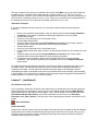
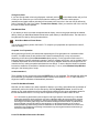
Masking Data
In this article, learn how to create and manipulate masks through both the worksheet and graph window.
The article is split up into four main sections:
•
•
•
•
The Mask toolbar | The Mask Toolbar Buttons | The Mask Shortcut Menus
Download Masking.EXE (required for Lesson 1 and Lesson 2)
Lesson 1 - Masking worksheet data for analysis
Lesson 2 - Masking data in a graph window for a linear fit
Note: This article was written using a feature first implemented in Origin 6.0. Users who have Origin 5.0 or
earlier will be unable to perform the activities included in Lessons 1 and 2. We encourage those users to
consider upgrading as soon as possible!
Introduction
The ability to mask data so that it is excluded from analysis is a new feature for Origin 6.0. Masking can
be performed on data in a worksheet or on the active data plot in a graph and can be applied to a single
data point or a range of points. When affecting a graph window, the new masking features can be applied
to active Scatter and Line + Symbol plots, but are technically not supported for any other plot types.
Masking is most useful when you want to exclude erroneous data points from analysis or when you only
want to analyze a specific subset of your data. The purpose of this article is to show you as much as
possible about how to use this new masking feature.
First, the Mask toolbar, its buttons, and the Mask shortcut menus are discussed. Then, two lessons are
provided. The first lesson focuses on masking and analyzing a set of quiz grades which have been
entered into an Origin worksheet. The second lesson focuses on masking and analyzing a randomly
generated dataset which has been plotted into a graph window. Before beginning either lesson you will
need to download Masking.EXE.
The Mask Toolbar
To enable the Mask toolbar, select View:Toolbars from the Origin menu bar. This opens the Customize
Toolbar dialog box. Make sure the Toolbars tab is selected. Then select the Mask toolbar by clicking
inside the check box next to the word Mask.
Note: Simply clicking the word Mask will not open the toolbar. You must click inside the check box.
If the check box contains a check mark, the toolbar is already available. Click OK to close out of the
Customize Toolbar dialog box when you are done. Here's what the Mask toolbar looks like:
Figure 1 - The Mask Toolbar
The Buttons
There are seven buttons on the Mask toolbar, each responsible for performing a different masking task.
Below is a description of what each button allows you to do, followed by an explanation of how to use the
button.
- Masked Point Toggle
Also called Point by Point on the Mask shortcut menu, the Masked Point Toggle button allows
you to mask and unmask a single data point from a graph window only.
After clicking on this button, the Data Reader tool activates. Double-click on the data point that
you want to mask. Once you do, the Data Reader closes and the data point becomes masked. To
indicate that the data point is masked, the symbol color changes to the current masking color.
The default masking color is red.
Note: Pressing the ESC key aborts the Mask Point Toggle activity.
- Mask Range
Also called Apply and Range on the Mask shortcut menus, the Mask Range button allows you to
mask a range of data in either a graph or worksheet window. For a graph window, the range you
pick is limited to the active data plot. For a worksheet window, the range can be any contiguous
group of cells in the worksheet, even if the selected range spans multiple columns.
To mask a range of data in a graph window, click on the Mask Range button. This activates the
Data Selector tool on the active data plot. Position the left and right Data Markers so that they
enclose the range you want to mask. Then, either press the ENTER key on your keyboard or
double-click on either of the Data Markers. This closes the Data Selector tool and masks the
defined range of data. Again, to delineate between masked and unmasked data, the masked data
displays using the current masking color.
When on a worksheet, highlight the desired range of data to be masked first, then click the Mask
Range button. This masks the data and displays all masked cells with the current masking color.
Note: Pressing the ESC key aborts the Mask Range activity. However, doing so does not
eliminate the Data Markers from view. To hide the Data Markers, simply select Data:Data
Markers.
- Unmask Range
Also referred to as Remove or Clear Range on some shortcut menus, the Unmask Range button
can be used to remove the mask from any range of data in either a worksheet or graph window.
The range that you specify does not necessarily have to be the entire range of data that is
masked and can be one single data point.
To unmask a range of data in a worksheet, select the desired range of data (or single cell) and
click the Unmask Range button.
To unmask a range of data in a graph window, activate the desired data plot and click on the
Unmask Range button. This activates the Data Selector tool. Position the Data Markers on the
first and last data points of the range you want to unmask. For a single data point, position both
Data Markers on the data point you want to unmask. Then, press the ENTER key on your
keyboard. This closes the Data reader tool and unmasks the selected data.
You may find that the Mask Point Toggle (discussed earlier) is much quicker and easier to use
when unmasking a single data point in a graph window.
Note: Pressing the ESC key aborts the Unmask Range activity. However, doing so does not
eliminate the Data Markers from view. To hide the Data Markers, simply select Data:Data
Markers.
- Swap Mask
The Swap Mask (or just Swap) button removes any masking present on the selected dataset and
applies it to that part of the selected dataset that was not originally masked. In other words, the
Swap Mask button reverses the masking of the selected dataset.
With a graph window active, select the desired dataset from the dataset list at the bottom of the
Data menu. Then click the Swap Mask button. With a worksheet window active, select the
desired dataset by clicking on the column title and click the Swap Mask button.
- Change Mask Color
Also referred to as Change Color, the Change Mask Color button changes the color of all masked
data project-wide. The default masking color is initially red, but once you change the masking
color within a project, the color you selected becomes the default masking color for the project
until it is changed again.
Once the button is clicked, the masking color increments by one to the next color in the color
palette list (Format:Color Palette). Although there are twenty-four colors in the color palette by
default, only twenty-three colors are used since this feature skips the first position in the color
pallete (normally black). Once the end of the color list is reached the cycle will begin all over
again.
- Hide/Show Masked Points
The Hide/Show Masked Points button toggles the display of all masked data in every graph
window contained in a project. The button will appear depressed when your masked data is
hidden and raised when your masked data is showing.
Note: If you have the Flat Toolbars check box enabled on the Toolbars tab of the Customize Toolbar
dialog box (View:Toolbars), this button will actually appear flat as opposed to raised if your masked
data is showing.
When hiding masked data, maintain a continuous line connection by enabling the Connect line
across Missing Data check box. This check box is located on the Display tab at the Graph level
of Plot Details. To get there, select Format:Page and then the Display tab (if it is not already
selected).
- Disable/Enable Masking
The Disable/Enable Masking button toggles the masking of all data in the project on or off. Its
state is remembered throughout an Origin session, but reverts back to being enabled if you exit
out of and then reopen Origin again. Similar to the Hide/Show Masked Points button, the
Disable/Enable Masking button will appear depressed when you have disabled masking and
raised (or flat as described above) when you have enabled masking. This button is especially
useful for observing the effects of including and excluding masked data from analysis without
having to actually remove a mask.
The Mask Shortcut Menus
Although the masking options cannot be accessed from Origin's main menus, you can mask your data via
shortcut menus. The actual masking features that are available from the Mask shortcut menu depend on
whether you intend to mask your data via the worksheet or the graph window.
The Worksheet
If you intend to mask your data via the worksheet, the masking options that are available are affected
further by the type of selection that has been made in the worksheet.
Selecting the entire worksheet
If you have selected the entire worksheet, the only masking options that are available are
Remove, Change Color, and Disable Masking (Figure 9). These selections are equivalent to the
Unmask Range, Change Mask Color, and Disable/Enable Masking buttons on the Mask toolbar.
The Remove option affects the entire worksheet while Change Color affects all masked data in
the project, and Disable Masking affects the entire Origin session.
Figure 9 - The Mask shortcut menu when an entire worksheet is selected
Selecting a worksheet column
If you have selected a worksheet column, the masking options that are available are Remove,
Swap, Change Color, and Disable Masking (Figure 10). These selections are equivalent to the
Unmask Range, Swap Mask, Change Mask Color, and Disable/Enable Masking buttons on the
Mask toolbar. Remove and Swap affect the current column selection only, while Change Color
affects all masked data in the project and Disable Masking affects the entire Origin session,
regardless of the current worksheet selection.
Figure 10 - The Mask shortcut menu when one column in a worksheet is selected
Selecting a range/single cell
If you select a range or single cell in a worksheet, the masking options that are available are
Apply, Remove, Change Color, and Disable Masking (Figure 11). These selections are equivalent
to the Mask Range, Unmask Range, Change Mask Color, and Disable/Enable Masking buttons
on the Mask toolbar. Apply and Remove affect the current selection only, while Change Color
affects all masked data in the project and Disable Masking affects the entire Origin session,
regardless of the current worksheet selection.
Figure 11 - The Mask shortcut menu when a range/single cell of a worksheet is selected
The Graph
All seven masking options are available when a graph window is active. The names are Point by
Point, Range, Clear Range, Swap, Change Color, Hide, and Disable Masking (Figure 12). These
selections are equivalent to the Masked Point Toggle, Mask Range, Unmask Range, Swap Mask,
Change Mask Color, Hide/Show Masked Points, and Disable/Enable Masking buttons on the
Mask toolbar. The first four options affect the active dataset only, while Change Color and Hide
affect all masked data in the project and Disable Masking affects the entire Origin session. The
active dataset can be determined by looking at the list of datasets in the Data menu. The dataset
preceded by a check mark is active.
Figure 12 - Active Dataset in a Graph Window
At this point you should be fully prepared to try out this new masking feature. However, before you begin
Lesson 1 make sure you download Masking.EXE.
Download
Lesson 1 and Lesson 2 are based on a project called Masking.OPJ. Before beginning, take a moment to
download a self-extracting *.EXE file which contains the project.
Download Masking.EXE (you will need to return to the article on our website to do this)
Save the *.EXE to a location of your choosing or accept the default (C:\). Next, open Windows Explorer
and navigate to where you have saved Masking.EXE. Double-click on the file to begin the extraction
process. Specify the location where you wish the file to be saved or accept the default (C:\) and click
Unzip. Finally, launch Origin 6.0 and open the project.
Project Setup
The project is separated into two subfolders called Lesson 1 and Lesson 2. To see the contents of
Lesson 1, double-click on it in Project Explorer.
Note: If you are unfamiliar with Project Explorer and/or would like to know more about it before continuing with
this article, take a look at the June 18, 1999 Technical Review called Understanding and Working with Layers Part 4 or consult the Origin User's Manual.
Once inside you will find that there is only one window contained in this folder. It is a worksheet called
Student. The worksheet consists of two columns called Quiz and Grade. Together, Quiz and Grade
describe a listing of ten quiz grades which a student received during one single term.
Now double-click on the Lesson 2 folder. You will find that Lesson 2 contains a worksheet window called
Flow and a graph window called RateVsTime. Flow contains two columns called Time and Rate. Time
contains the times (in hours) at which each Rate measurement was taken. Rate contains flow rate
readings (in ft3/sec) for a bypass pipeline in a dam.
Now that you have familiarized yourself with the project, move on to Lesson 1.
Lesson 1
Purpose
The primary purpose of this lesson is to show you how to impose and manipulate a mask on a dataset
contained in a worksheet. In addition to this, the lesson will also illustrate the effect a mask has when
calculating the statistics of a dataset and when plotting a Box Chart.
Getting Started
Both Lesson 1 and Lesson 2 are based on a project file called Masking.OPJ. If you have not downloaded
Masking.EXE, please do so now. Once the download is complete, open Masking.OPJ and select the
Lesson 1 subfolder (if you are not there already) to begin the lesson.
Setting Up the Worksheet
Suppose you are the student who took the 10 quizzes and you want to perform some simple analysis on
them. Specifically, you are interested in how largely affected your quiz average would be if the lowest
grade (32) or the two lowest grades (32 and 62) were dropped.
In order to compare these two possibilities against the average for all 10 grades, create two additional
columns consisting of the same Grade data. To do so, select Column:Add New Columns, enter a value
of 2, and click OK. This adds a third and fourth column to the worksheet. The columns should
automatically be named A and B, respectively and are referred to as such during this lesson.
Next, copy and paste the quiz grades into columns A and B. To do so, select the 10 values in the Grade
column and then the Edit:Copy menu command. Then, click on the first cell in column A and select
Edit:Paste. Similarly, click on the first cell in column B and select Edit:Paste.
Masking
Since there are now three columns with the same data, you can use the Grade column to calculate the
average of all 10 quiz grades while the other two columns, A and B, can be used to calculate the average
for the top 9 and the top 8 quiz grades, respectively.
To mask the cell containing the 32 in column A, click on the cell and then on the Mask Range button on
the Mask toolbar. As mentioned previously, the Mask Point Toggle feature is not available for worksheets.
Alternatively, right-click on the cell containing the 32 and select Mask:Apply. To mask the range of cells
containing the 32 and 62 in column B, click inside one of the cells and drag until both cells are selected.
Then, as done previously, click the Mask Range button or select Mask:Apply from the shortcut menu.
Now you are ready to analyze the data.
Statistics on Columns
Select all three columns (Grade, A, and B) by clicking and dragging across all three column titles. Then,
select Analysis:Statistics on Columns. Since you selected all three columns at once, the statistics for
each column are placed in the same worksheet in separate rows.
Compare the Results
With the statistics for all three columns in one worksheet, comparing the average is easy.
The quiz average for each column is contained in the column called Mean. As you can see by looking at
the Mean for row 1, calculating the average using all 10 values results in a 77. That's a C+ by most
grading standards. However, if you remove the lowest grade from the average, the result quickly jumps to
an 82 (as seen in the Mean column for row 2), or a B-. Finally, if you exclude the two lowest grades from
the average the result is an 84.5 (as seen in the Mean column for row 3), or a B.
Alternative Technique
If you hadn't created the two extra columns, you could have achieved similar results by doing the
following:
Return to the worksheet called Student, select the Grade column and then Analysis:Statistics
on Columns. This creates a worksheet containing the statistics for all 10 quiz grades.
2. Activate Student again.
3. Click on the cell containing the 32 in the Grade column.
4. Click the Mask Range button.
5. Select the Grade column and then Analysis:Statistics on Columns. This creates a another
worksheet which contains the statistics for the 9 remaining quiz grades.
6. Activate Student again.
7. Click on the cell containing the 62 in the Grade column.
8. Click the Mask Range button again. Since the 32 was already masked it is not necessary to mask
it again.
9. Select the Grade column and then Analysis:Statistics on Columns. This creates a third
worksheet which contains the statistics for the 8 remaining quiz grades.
10. Compare the value contained in the first cell of the Mean column for the three statistical
worksheets. They should be equivalent to the explanation found in the Compare the Results
section above.
1.
The difference between this alternative technique and the first is that by manipulating the mask on only
the Grade column, the alternative technique forces you to switch between statistical worksheets to
compare the averages. For this reason the alternative technique might not be desirable. However,
manipulating the mask on the Grade column when it is plotted as a box chart is actually quite interesting.
It actually allows you to make quick comparisons of the averages through the graphical representation of
Grade's statistics. To see what I mean, continue reading.
Lesson 1 - (continued)
Plot Grade as a Box Chart
First, if necessary unmask the 32 and 62 in the Grade column by selecting the two cells and clicking the
Unmask Range button. Alternatively, right-click on the entire Grade column and select Mask:Remove.
Either method removes the mask on the two grades. Then, with the Grade column still selected, select
Plot:Statistical Graphs:Box Chart or click on Box Chart button (seen below) on the 2D Graphs
Extended toolbar (View:Toolbars). This plots a box chart representing the statistics calculated for all 10
grades.
- Box Chart Button
Enable the Labels
Double-click on the box chart to bring up Plot Details. Select the Box tab and enable the Box and Whisker
Labels check boxes. Select the Label tab and change the Size drop-down list to a larger value (e.g. 22).
Click OK to apply and view the changes. Enabling and altering these features will make the effects of
masking on the box chart more obvious.
Mask the Data
Now, return to the Student worksheet. Position the worksheet so that you can also see the box chart.
Mask the 32 in the Grade column. Notice that the appearance of the box chart automatically changes to
reflect the omission of the 32. Now mask the 62. The box chart should again update to reflect the newly
masked data point. The fact that the box chart changes each time a different mask is implemented makes
it easy to see the effect each mask has on the average. It also eliminates the need to plot each mask as a
separate box chart!
This completes Lesson 1. Continue on to Lesson 2 to learn about masking data plotted in the graph
window.
Lesson 2
Purpose
The primary purpose of this lesson is to show you how to impose and manipulate a mask on a dataset
contained in a graph window. In addition to this, the lesson will also illustrate the effect a mask has when
performing a linear fit on the data plot.
Getting Started
As stated previously, both Lesson 1 and Lesson 2 are based on a project file called Masking.OPJ. If you
have not already done so, download Masking.EXE. Once you have downloaded the project, open it in
Origin and double-click on the Lesson 2 subfolder. As mentioned on the download page, Lesson 2
contains a worksheet called Flow and a graph called RateVsTime.
RateVsTime is a graphical representation of the flow rate of water passing through a pipeline called
Bypass #1 in a dam. Occasionally there are leaks and/or periods when a second pipeline (Bypass #2) is
brought on line to handle unexpected influxes of water. These data points are indicated by the arrows.
Mask Data Points
Suppose you are a worker at this dam and you need to determine the flow increase per hour
(ft.3/sec/hour) of the water flowing through Bypass #1 for a report that you are preparing. To do so, all you
need to do is perform a linear fit on the data and obtain the slope. However, in order for the fit to be valid,
you must eliminate the lower readings due to leaks and Bypass #2 being brought on line. Rather than
physically removing these lower readings from the Flow worksheet, mask them directly in RateVsTime.
To begin masking, make the graph active and then click on
on the Mask toolbar. Then, double-click
on the leftmost point which is next to an arrow and to the left of the dashed vertical line (X=9.47266,
Y=301.234). Alternatively, click once on that point and press the ENTER key on your keyboard. Either
method masks that point and changes its color to denote the masked state. Mask the second point to the
left of the dashed line in a similar manner (X=17.2955, Y=578.954).
To mask the points to the right of the dashed vertical line, click on the Mask Range button
. This
activates the Data Reader tool and displays the data makers at either end of the active data plot. With
your mouse, click and drag the left data marker until it is on top of the first data point after the dashed
vertical line (X=23.13426, Y=664.907). Then, either double-click on that point or press the ENTER key.
Either method masks the entire range of data and changes the color of that data to the current masking
color.
If you now return to the RateVsTime worksheet you will see that the masks you have just imposed are
displayed as such there, too.
Change the Color
If you don't like the mask color being displayed, continually click on
on the Mask toolbar until you find
a color you like. Each time you click on this button the masking color used in the entire project
(worksheets and graph windows included) will increment to the next color in the color list (as defined by
colors 2 through 24 in the Color Palette - Format:Color Palette). When you reach the end of the color list
the cycle of colors will be repeated.
Hide Masked Data
If you decide you don't even want the masked data to display, return to the graph and hide the masked
data by clicking on Hide/Show Masked Points button (seen below) on the Mask toolbar. The data can be
brought back into view by clicking the same button.
- Hide/Show Masked Points Button
You are almost ready to perform the linear fit. To complete your preparation and perform the linear fit,
continue reading.
Complete Your Preparation
When performing a linear fit, the dataset that represents the fit line gets placed in a worksheet called
LinearFit. If multiple linear fits are performed the LinearFit worksheet may or may not increment
depending on the value of the create.enumwks object property. For the purposes of this lesson it is
important that the LinearFit worksheet increment in order to compare two fit lines, one for the data when it
is masked and another when the mask has been removed or disabled. Otherwise the second fit line will
overwrite the first, making comparisons between the two difficult. To ensure that the LinearFit worksheet
increments, enable the enumeration of worksheets manually. To do so, select Window:Script Window
and type in the following line of script:
create.enumwks=1;
Then, highlight the line of script and press the ENTER key on your keyboard. The datasets that define the
two fit lines will get outputted to worksheets called LinearFit1 and LinearFit2. Note: In later versions of
Origin the LinearFit worksheet will automatically increment.
Linear Fit With Mask Enabled
Now that you have masked your data, adjusted its display to your liking, and enabled the enumeration of
worksheets, perform the linear fit on the data plot by selecting Analysis:Fit Linear. A red fit line will
appear on your graph window as well as a legend which contains the plot types and dataset names for
the raw data and the linear fit. You may want to reposition the legend to make it easier to read.
Note: The Results Log (View:Toolbars) will also appear in the Origin workspace. The Results Log is a dockable
window that contains the results of the linear fit as well as a date/time stamp, the project file location, the name
of the dataset the analysis was performed on, and the type of analysis performed. If the Results Log window is
restricting your view of the graph, simply click on its title bar and drag it to another location. To prevent if from
becoming docked, hold down the CTRL key while dragging it. If it becomes docked (but you do not want it
docked), undock it by double-clicking on the two vertical lines on the left side of the window. You can also close
the Results Log by undocking it and clicking on the X button or by selecting View:Toolbars and de-selecting it
from the list on the Toolbars tab.
Linear Fit With Mask Removed or Disabled
At this point you might be wondering if the masked data was in fact ignored during the fit. To determine
this either remove all masks that you have imposed on your dataset or disable them and perform a
second linear fit on the data.
To remove all masks on the plot click on
on the Mask toolbar. When the data markers appear on the
graph simply press the ENTER key on your keyboard. Any masks occurring on the entire dataset are
removed as is indicated by the symbol color change.
on the Mask toolbar. All
To disable the masks you have imposed on the data plot simply click on
masks existing on the dataset as well as the entire project are disabled until you click this button again.
Once you have successfully removed or disabled the masks on the dataset, select Analysis:Fit Linear
again. Another red fit line will appear on the graph and the legend will automatically update to include the
new fit line plot type and dataset name. The Results Log will also update to include the results of the
second fit. At this point if you take a look at the two fit lines you should clearly see that the masked data
was not considered in the initial fit.
Since the masked data was in fact ignored in the first fit you can use the slope of that fit for your report.
To find the slope, simply locate the result for parameter B of the first fit in the Results Log. It should be
34.72482. Now that the slope has been found, make some finishing touches on the graph so that it can
be included in the report.
Making the Finishing Touches
1.
2.
3.
Double-click on the legend to bring up the Text Control dialog box.
Replace all text with the following, regardless of which scenario (1 or 2) occurred:
\L(1) Valid Data
\L(1,8) Masked Points
\L(2) %(2)
Click Ok to close out of the Text Control dialog box.
Once you have completed the legend changes, remove the second fit line from the graph window (if there
is one) by deleting the hidden worksheet called LinearFit2. To do so, open Project Explorer (if it is not
already open) by selecting View:Project Explorer. Then, right-click on LinearFit2 and select Delete
Window. If the second fit updated the first fit line as in scenario 2, this step is not necessary. Instead, reapply or enable the masks created in the Mask Data Points section and perform the linear fit again.
Doing so will replace the second instance of the fit line with the original version from the first fit. At this
point the graph is ready for presentation.
A Note About Printing With Masked Data
In order to include the graph along with the report you may want to print it out. Since the graph contains
masked data, keep in mind that Origin handles masked data as one would expect.
If the masked data is:
• Hidden - the data will remain hidden in the printout unless the mask is disabled (see Disabled
below).
• Shown - the data will show in the printout and will print using the current masking color unless
disabled (see Disabled below).
• Disabled - the data will print out using the current symbol color as selected for that data plot in
Plot Details.
• Enabled - the data will print out using the current masking color unless hidden (see Hidden
above).
This completes Lesson 2.