Download EC-Lab software Techniques and Applications manual


EC-Lab Software:
Techniques
and Applications
Version 10.1x – February 2011
ii
Equipment installation
WARNING !: The instrument is safety ground to the Earth through the protective
conductor of the AC power cable.
Use only the power cord supplied with the instrument and designed for the good
current rating (10 Amax) and be sure to connect it to a power source provided with
protective earth contact.
Any interruption of the protective earth (grounding) conductor outside the instrument
could result in personal injury.
Please consult the installation manual for details on the installation of the instrument.
General description
The equipment described in this manual has been designed in accordance with EN61010
and EN61326 and has been supplied in a safe condition. The equipment is intended for
electrical measurements only. It should be used for no other purpose.
Intended use of the equipment
This equipment is an electrical laboratory equipment intended for professional and intended
to be used in laboratories, commercial and light-industrial environments. Instrumentation and
accessories shall not be connected to humans.
Instructions for use
To avoid injury to an operator the safety precautions given below, and throughout the
manual, must be strictly adhered to, whenever the equipment is operated. Only advanced
user can use the instrument.
Bio-Logic SAS accepts no responsibility for accidents or damage resulting from any failure to
comply with these precautions.
GROUNDING
To minimize the hazard of electrical shock, it is essential that the equipment be connected to
a protective ground through the AC supply cable. The continuity of the ground connection
should be checked periodically.
ATMOSPHERE
You must never operate the equipment in corrosive atmosphere. Moreover if the equipment
is exposed to a highly corrosive atmosphere, the components and the metallic parts can be
corroded and can involve malfunction of the instrument.
The user must also be careful that the ventilation grids are not obstructed. An external
cleaning can be made with a vacuum cleaner if necessary.
Please consult our specialists to discuss the best location in your lab for the instrument
(avoid glove box, hood, chemical products, …).
i
AVOID UNSAFE EQUIPMENT
The equipment may be unsafe if any of the following statements apply:
- Equipment shows visible damage,
- Equipment has failed to perform an intended operation,
- Equipment has been stored in unfavourable conditions,
- Equipment has been subjected to physical stress.
In case of doubt as to the serviceability of the equipment, don’t use it. Get it properly checked
out by a qualified service technician.
LIVE CONDUCTORS
When the equipment is connected to its measurement inputs or supply, the opening of
covers or removal of parts could expose live conductors. Only qualified personnel, who
should refer to the relevant maintenance documentation, must do adjustments, maintenance
or repair
EQUIPMENT MODIFICATION
To avoid introducing safety hazards, never install non-standard parts in the equipment, or
make any unauthorised modification. To maintain safety, always return the equipment to
Bio-Logic SAS for service and repair.
GUARANTEE
Guarantee and liability claims in the event of injury or material damage are excluded when
they are the result of one of the following.
- Improper use of the device,
- Improper installation, operation or maintenance of the device,
- Operating the device when the safety and protective devices are defective
and/or inoperable,
- Non-observance of the instructions in the manual with regard to transport,
storage, installation,
- Unauthorized structural alterations to the device,
- Unauthorized modifications to the system settings,
- Inadequate monitoring of device components subject to wear,
- Improperly executed and unauthorized repairs,
- Unauthorized opening of the device or its components,
- Catastrophic events due to the effect of foreign bodies.
ii
IN CASE OF PROBLEM
Information on your hardware and software configuration is necessary to analyze and finally
solve the problem you encounter.
If you have any questions or if any problem occurs that is not mentioned in this document,
please contact your local retailer (list available following the link Erreur ! Référence de lien
hypertexte non valide.). The highly qualified staff will be glad to help you.
Please keep information on the following at hand:
- Description of the error (the error message, mpr file, picture of setting or
any other useful information) and of the context in which the error
occurred. Try to remember all steps you had performed immediately
before the error occurred. The more information on the actual situation you
can provide, the easier it is to track the problem.
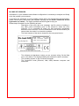
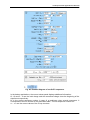
- The serial number of the device located on the rear panel device.
Model: VMP3
s/n°: 0001
Power: 110-240 Vac 50/60 Hz
Fuses: 10 AF Pmax: 650 W
-
The software and hardware version you are currently using. On the Help
menu, click About. The displayed dialog box shows the version numbers.
The operating system on the connected computer.
The connection mode (Ethernet, LAN, USB) between computer and
instrument.
iii
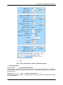
General safety considerations
The instrument is safety ground to the Earth through
the protective conductor of the AC power cable.
Class I
Use only the power cord supplied with the instrument
and designed for the good current rating (10 A max)
and be sure to connect it to a power source provided
with protective earth contact.
Any interruption of the protective earth (grounding)
conductor outside the instrument could result in
personal injury.
Guarantee and liability claims in the event of injury or
material damage are excluded when they are the result of
one of the following.
- Improper use of the device,
- Improper installation, operation or maintenance of the
device,
- Operating the device when the safety and protective
devices are defective and/or inoperable,
- Non-observance of the instructions in the manual with
regard to transport, storage, installation,
- Unauthorised structural alterations to the device,
- Unauthorised modifications to the system settings,
- Inadequate monitoring of device components subject
to wear,
- Improperly executed and unauthorised repairs,
- Unauthorised opening of the device or its components,
- Catastrophic events due to the effect of foreign bodies.
ONLY QUALIFIED PERSONNEL should operate (or
service) this equipment.
iv
Techniques and Applications Manual
Table of contents
Equipment installation
General description
Intended use of the equipment
Instructions for use
General safety considerations
i
i
i
i
iv
1.
Introduction........................................................................................................................ 4
2.
Electrochemical Techniques ............................................................................................ 5
2.1
Voltamperometric techniques .................................................................................... 5
2.1.1 OCV: Open Circuit Voltage ...................................................................................... 5
2.1.2 CV: Cyclic Voltammetry ........................................................................................... 5
2.1.3 CVA: Cyclic Voltammetry Advanced ...................................................................... 11
2.1.4 Linear Sweep Voltammetry: LSV............................................................................ 15
2.1.5 Chrono I/Q: Chronoamperometry / Chronocoulometry ........................................... 16
2.1.6 CP: Chronopotentiometry ....................................................................................... 20
2.1.7 SV: Staircase Voltammetry .................................................................................... 23
2.1.8 LASV: Large Amplitude Sinusoidal Voltammetry .................................................... 26
2.1.9 Alternating Current Voltammetry (ACV).................................................................. 28
2.2
Electrochemical Impedance Spectroscopy .............................................................. 30
2.2.1 Principles of multisine measurements .................................................................... 30
2.2.2 PEIS: Potentiostatic Impedance ............................................................................. 32
2.2.2.1 Description ..................................................................................................... 32
2.2.2.2 Additional features: ......................................................................................... 35
2.2.3 GEIS: Galvanostatic Impedance ............................................................................ 35
2.2.4 Visualisation of impedance data files ..................................................................... 37
2.2.4.1 Standard visualisation modes ......................................................................... 37
2.2.4.2 Counter electrode EIS data plot ...................................................................... 39
2.2.4.3 Frequency vs. time plot .................................................................................. 40
2.2.5 Staircase Electrochemical Impedance Spectroscopy ............................................. 42
2.2.5.1 SGEIS: Staircase Galvano Electrochemical Impedance Spectroscopy ........... 42
2.2.5.2 SPEIS: Staircase Potentio Electrochemical Impedance Spectroscopy ........... 45
2.2.5.2.1 Description
45
2.2.5.2.2 Application
48
2.3
Pulses ..................................................................................................................... 50
2.3.1 DPV: Differential Pulse Voltammetry ...................................................................... 50
2.3.2 SWV: Square Wave Voltammetry .......................................................................... 53
2.3.3 DNPV: Differential Normal Pulse Voltammetry ....................................................... 55
2.3.4 NPV: Normal Pulse Voltammetry ........................................................................... 57
2.3.5 RNPV: Reverse Normal Pulse Voltammetry ........................................................... 59
2.3.6 DPA: Differential Pulse Amperometry..................................................................... 61
2.4
Technique Builder ................................................................................................... 64
2.4.1 MG: Modular Galvano ............................................................................................ 64
2.4.1.1 Open Circuit Voltage (Mode = 0) .................................................................... 65
2.4.1.2 Galvanostatic (Mode = 1) ............................................................................... 66
2.4.1.3 Galvanodynamic (Mode = 2) .......................................................................... 67
2.4.1.4 Sequences with the Modular galvano technique ............................................. 68
2.4.2 MP: Modular Potentio............................................................................................. 68
2.4.2.1 Open Circuit Voltage (Mode = 0) .................................................................... 69
2.4.2.2 Potentiostatic (Mode = 1)................................................................................ 70
2.4.2.3 Potentiodynamic (Mode = 2) ........................................................................... 71
1
Techniques and Applications Manual
2.4.3 Triggers.................................................................................................................. 72
2.4.4 The Wait Option ..................................................................................................... 74
2.4.5 Temperature Control – TC ..................................................................................... 74
2.4.6 Rotating Disk Electrode Control – RDEC ............................................................... 75
2.4.7 External Device Control –EDC ............................................................................... 77
2.4.8 The Loop option ..................................................................................................... 77
2.4.9 The Pause technique ............................................................................................. 78
2.5
Manual Control ........................................................................................................ 79
2.5.1 Potential Manual Control ........................................................................................ 79
2.5.2 Current Manual Control .......................................................................................... 79
2.6
Ohmic Drop Determination ...................................................................................... 80
2.6.1 MIR: manual IR compensation ............................................................................... 80
2.6.2 ZIR: IR compensation with EIS .............................................................................. 80
2.6.3 CI: Current Interrupt ............................................................................................... 81
3.
Electrochemical applications ......................................................................................... 83
3.1
Battery .................................................................................................................... 83
3.1.1 PCGA: Potentiodynamic Cycling with Galvanostatic Acceleration .......................... 83
3.1.1.1 Description of a potentiodynamic sequence ................................................... 85
3.1.1.2 Description of the cell characteristics window for batteries ............................. 87
3.1.1.3 PCGA Data processing .................................................................................. 88
3.1.1.3.1 Compact function
88
3.1.1.3.2 Intercalation coefficient determination
89
3.1.2 GCPL: Galvanostatic Cycling with Potential Limitation ........................................... 90
3.1.2.1 Description of a galvanostatic sequence......................................................... 92
3.1.2.2 Application ...................................................................................................... 94
3.1.2.3 GCPL Data processing: .................................................................................. 95
3.1.2.3.1 Compacting process for the apparent resistance determination
95
3.1.3 GCPL2: Galvanostatic Cycling with Potential Limitation 2 ...................................... 95
3.1.4 GCPL3: Galvanostatic Cycling with Potential Limitation 3 ...................................... 97
3.1.5 GCPL4: Galvanostatic Cycling with Potential Limitation 4 ...................................... 98
3.1.6 GCPL5: Galvanostatic Cycling with Potential Limitation 5 .................................... 100
3.1.6.1 Description of a galvanostatic sequence....................................................... 102
3.1.6.2 GCPL5 Data processing ............................................................................... 103
3.1.6.3 Application: ................................................................................................... 103
3.1.7 GCPL6: Galvanostatic Cycling with Potential Limitation 6 .................................... 104
3.1.7.1 Description of a galvanostatic sequence....................................................... 105
3.1.8 CLD: Constant Load Discharge ............................................................................ 107
3.1.9 CPW: Constant Power ......................................................................................... 109
3.1.9.1 Description ................................................................................................... 109
3.1.9.2 Application of the CPW technique ................................................................ 111
3.1.10
APGC: Alternate Pulse Galvano Cycling .......................................................... 114
3.1.11
PPI: Potentio Profile Importation....................................................................... 117
3.1.12
GPI: Galvano Profile Importation ...................................................................... 119
3.1.13
RPI: Resistance Profile Importation .................................................................. 120
3.1.14
PWPI: Power Profile Importation ...................................................................... 120
3.2
Photovoltaics / Fuel Cells ...................................................................................... 121
3.2.1 I-V Characterization: IVC...................................................................................... 122
3.2.1.1 Description ................................................................................................... 123
3.2.1.2 Process ........................................................................................................ 124
3.2.2 Constant load discharge ...................................................................................... 124
3.2.3 CPW: Constant Power ......................................................................................... 126
3.2.4 Constant Voltage : CstV ....................................................................................... 127
2
Techniques and Applications Manual
3.2.5 Constant Current : CstC ....................................................................................... 129
3.3
Corrosion .............................................................................................................. 131
3.3.1 EVT: Ecorr versus Time ......................................................................................... 131
3.3.2 LP: Linear Polarization ......................................................................................... 132
3.3.2.1 Description ................................................................................................... 132
3.3.2.2 Process and fits related to LP ....................................................................... 133
3.3.3 CM: Corrosimetry (Rp vs. Time) ........................................................................... 133
3.3.3.1 Description ................................................................................................... 134
3.3.3.2 Applications of the Corrosimetry application ................................................. 136
3.3.4 VASP: Variable Amplitude Sinusoidal microPolarization ...................................... 137
3.3.5 CASP: Constant Amplitude Sinusoidal microPolarization ..................................... 138
3.3.6 GC: Generalized Corrosion .................................................................................. 139
3.3.6.1 Description ................................................................................................... 141
3.3.6.2 Process and fits related to GC ...................................................................... 142
3.3.7 CPP: Cyclic Potentiodynamic Polarization ........................................................... 143
3.3.8 Dep. Pot.: Depassivation Potential ....................................................................... 146
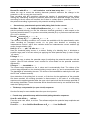
3.3.9 CPT: Critical Pitting Temperature ......................................................................... 149
3.3.9.1 Differences in the CPT technique between the VMP and the other
instruments .................................................................................................................. 149
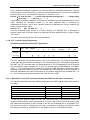
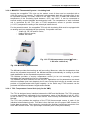
3.3.9.2 MINISTAT Thermostat/Cryostat - circulating bath......................................... 150
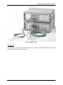
3.3.9.3 TCU: Temperature Control Unit (only for the VMP) ...................................... 150
3.3.9.4 CPT Technique ............................................................................................ 152
3.3.9.5 CPT2 technique............................................................................................ 157
3.3.10
MPP: Multielectrode Potentiodynamic Pitting ................................................... 161
3.3.10.1
Description ............................................................................................... 163
3.3.10.2
Data processing........................................................................................ 165
3.3.11
MPSP: Multielectrode Potentiostatic Pitting ...................................................... 165
3.3.12
ZRA: Zero Resistance Ammeter ....................................................................... 167
3.3.13
ZVC: Zero Voltage Current ............................................................................... 169
3.4
Custom Applications ............................................................................................. 171
3.4.1 MUIC: Measurement of U-I Correlations .............................................................. 171
3.4.2 PR: Polarization Resistance ................................................................................. 171
3.4.3 SPFC: Stepwise Potential Fast Chronoamperometry ........................................... 175
3.4.4 PEISW: Potentio Electrochemical Impedance Spectroscopy Wait ........................ 177
3.4.5 How to add a homemade experiment to the custom applications ......................... 178
3.5
Special applications .............................................................................................. 179
3.5.1 SOCV: Special Open Circuit Voltage ................................................................... 181
3.5.2 SMP: Special Modular Potentio ............................................................................ 182
3.5.3 Special Modular Galvano ..................................................................................... 187
3.5.4 SGCPL: Special Galvanostatic Cycling with Potential Limitation .......................... 190
4.
Linked experiments ....................................................................................................... 194
4.1
4.2
4.3
Description and settings ........................................................................................ 194
Example of linked experiment ............................................................................... 195
Application ............................................................................................................ 196
5.
Stack experiments ......................................................................................................... 199
6.
Summary of the available techniques and applications in EC-Lab .......................... 204
7.
List of abbreviations used in EC-Lab software .......................................................... 206
8.
Glossary ......................................................................................................................... 208
9.
Index ............................................................................................................................... 212
3
Techniques and Applications Manual
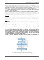
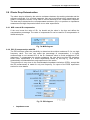
1.
Introduction
EC-Lab software has been designed and built to control all of our potentiostats (single or
multichannel: SP-50 SP-150, SP-200 and SP-300, MPG, MPG2, VMP, VMP2(Z), BiStat,
VMP3, VSP, HCP-803, HCP-1005, CLB-500, EPP-400 and EPP-4000). Each channel board
of our multichannel instruments is an independent potentiostat/galvanostat that can be
controlled by EC-Lab software.
Each channel can be set, run, paused or stopped, independently of each other, using
identical or different techniques. Any settings of any channel can be modified during a run,
without interrupt the experiment. The channels can be interconnected and run
synchronously, for example to perform multi-pitting experiments using a common counterelectrode in a single bath.
One computer (or several for multichannel instruments) connected to the instrument monitor
the system. The computer connects to the instrument through an Ethernet connection or with
an USB connection. With the Ethernet connection, each one of the users is able to monitor
his own channel from his computer. More than multipotentiostats, our instruments are
modular, versatile and flexible multi-user instruments.
Once the techniques have been loaded and started from the PC, the experiments are entirely
controlled by the instrument’s on-board firmware. Data are temporarily buffered in the
instrument and regularly transferred to the PC, which is used for data storage, on-line
visualization, and off-line data analysis and display. This architecture ensures a very safe
operation since a shut down of the monitoring PC does not affect the experiments in
progress.
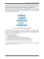
The application software package provides useful techniques separated into two categories
Electrochemical Techniques and Electrochemical Applications. The techniques contain
general voltamperometric (Cyclic Voltammetry, Chronopotentiometry), differential
techniques, impedance techniques, and a technique builder including modular potentio and
galvano, triggers, wait, and loop options. The applications are made of techniques more
dedicated to specific fields of electrochemistry such as battery, fuel cells, super-capacitors
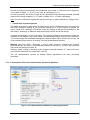
testing, corrosion study, and custom applications. Electrochemical techniques and
applications are obtained by associations of elementary sequences (blocks) and appear as
flow diagrams combining these sequences. The settings can also be displayed as column
setup.
Conditional tests can be performed at various levels of any sequence on either the working
electrode potential, current, or on the counter electrode potential, or on the external
parameters. These conditional tests force the experiment to go to the next step, loop to a
previous sequence or end the sequence.
The aim of this manual is to describe every technique and application available in the
EC-Lab software. This manual composed of several chapters. The first is an introduction.
The second section describes electrochemical techniques, and the third explains
electrochemical applications. The fourth part details how to build complex experiments as
linked techniques.
©
It is assumed that the user is familiar with Microsoft Windows and knows how to use the
mouse and keyboard to access the drop-down menus.
WHEN A USER RECEIVES A NEW UNIT FROM THE FACTORY, THE SOFTWARE AND FIRMWARE ARE
INSTALLED AND UPGRADED. THE INSTRUMENT IS READY TO BE USED. IT DOES NOT NEED TO BE
UPGRADED. WE ADVISE THE USERS TO READ AT LEAST THE SECOND AND THIRD CHAPTERS OF THIS
DOCUMENT BEFORE STARTING AN EXPERIMENT.
4
Techniques and Applications Manual
2.
Electrochemical Techniques
2.1 Voltamperometric techniques
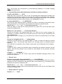
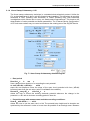
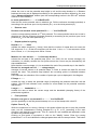
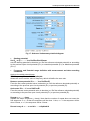
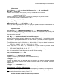
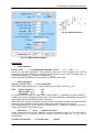
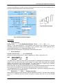
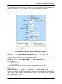
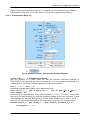
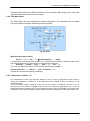
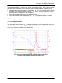
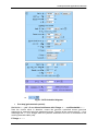
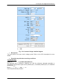
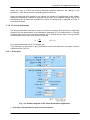
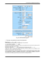
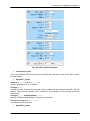
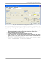
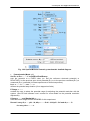
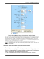
2.1.1 OCV: Open Circuit Voltage
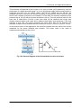
The Open Circuit Voltage (OCV) consists of a period during which no potential or current is
applied to the working electrode. The cell is disconnected from the power amplifier. On the
cell, the potential measurement is available. Therefore the evolution of the rest potential can
be recorded. This period is commonly used as preconditioning time or for equilibration of the
electrochemical cell.
Fig. 1: Open Circuit Voltage Technique.
Rest for tR =
h
mn
s
fixes a defined time duration tR for recording the rest potential.
or until |dEwe/dt| < |dER/dt| =
mV/h
stops the rest sequence when the slope of the open circuit potential with time, |dER/dt|
becomes lower than the set value (value 0 invalidates the condition).
Record Ewe every dER =
mV resolution and at least every dtR =
s
allows the user to record the working electrode potential whenever the change in the
potential is  dER with a minimum recording period in time dtR.
Data recording with dER resolution can reduce the number of experimental points without
loosing any "interesting" changes in potential. When there is no potential change, only points
according to the dtR value are recorded but if there is a sharp peak in potential, the rate of
recording increases.
E Range = …….
enables the user to select the potential range for adjusting the potential resolution with his
system. (See EC-Lab software user’s manual for more details on the potential resolution
adjustment)
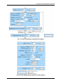
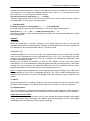
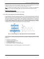
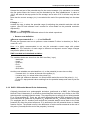
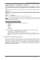
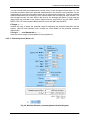
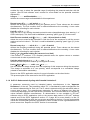
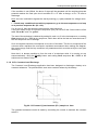
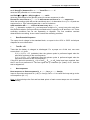
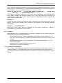
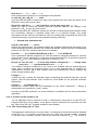
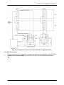
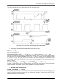
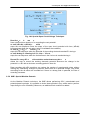
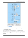
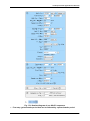
2.1.2 CV: Cyclic Voltammetry
Cyclic voltammetry (CV) is the most widely used technique for acquiring qualitative
information about electrochemical reactions. CV provides information on redox processes,
heterogeneous electron-transfer reactions and adsorption processes. It offers a rapid
location of redox potential of the electroactive species.
5
Techniques and Applications Manual
CV consists of linearly scanning the potential of a stationary working electrode using a
triangular potential waveform. During the potential sweep, the potentiostat measures the
current resulting from electrochemical reactions (consecutive to the applied potential). The
cyclic voltammogram is a current response as a function of the applied potential.
Traditionally, this technique is performed using a straight analog ramp. Due to the digital
nature of the potentiostat, however, the actual ramp applied consists of a series of small
potential steps that approximate the linear ramp desired (see the control potential resolution
part in the EC-Lab software manual)
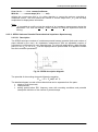
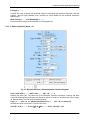
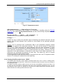
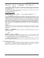
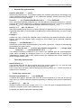
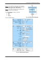
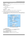
Fig. 2: General diagram for Cyclic Voltammetry.
The "Cyclic Voltammetry" technique has been briefly detailed in the EC-Lab software
manual. This technique corresponds to normal cyclic voltammetry, using a digital potential
staircase i.e. it runs defined potential increment regular in time. The software adjusts the
potential step to be as small as possible.
The technique is composed of:
 a starting potential setting block,
 a 1st potential sweep with a final limit E1,
 a 2nd potential sweep in the opposite direction with a final limit E2,
 the possibility to repeat nc times the 1st and the 2nd potential sweeps,
 a final conditional scan reverse to the previous one, with its own limit EF.
Note that all the different sweeps have the same scan rate (absolute value).
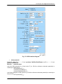
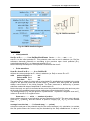
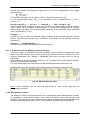
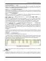
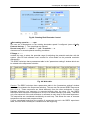
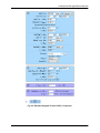
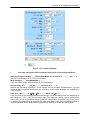
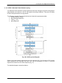
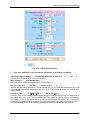
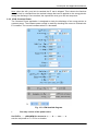
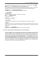
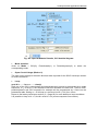
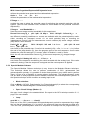
The detailed flow diagram (on the following figure) is made of five blocks (it is also possible
to display the column diagram Fig. 4):
6
Techniques and Applications Manual
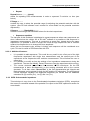
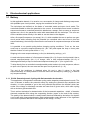
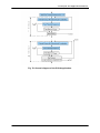
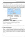
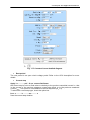
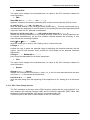
Fig. 3: Cyclic Voltammetry detailed flow diagram.
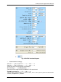
Fig. 4: Cyclic Voltammetry detailed column diagram.
7
Techniques and Applications Manual
 Starting potential
Set Ewe to Ei = …….. V vs Ref/Eoc/Ectrl/Emeas
sets the starting potential in absolute (vs. Ref, the reference electrode potential in the cell) or
according to the previous open circuit potential (Eoc) or controlled potential (Ectrl) or Measured
potential (Emeas).
 First potential sweep with measurement and data recording conditions
Scan Ewe with dE/dt = ……. mV/s ( 300 µV/15 ms)
allows the user to set the scan rate in mV/s The potential step height and its duration are
optimized by the software in order to be as close as possible to an analogic scan. Between
brackets the potential step height and the duration are displayed according to the potential
resolution defined by the user in the “Advanced Settings” window (see the corresponding
section in the EC-Lab software manual).
to vertex potential E1 = ……. V vs Ref/Eoc/Ei.
fixes the first vertex potential value in absolute (vs. Ref) or according to the previous open
circuit potential (Eoc), or according to the potential of the previous experiment (Ei).
Measure <I> over the last ……. % of the step duration
selects the end part of the potential step (from 1 to 100%) for the current average (<I>)
calculation, to possibly exclude the first points where the current may be disturbed by the
step establishment.
Note that the current average (<I>) is recorded at the end of the potential step to the data file.
Record <I> averaged over N = ……. voltage step(s)
averages N current values on N potential steps, in order to reduce the data file size and
smooth the trace. The potential step between two recording points is indicated between
brackets.
Once selected, an estimation of the number of points per cycle is displayed in the diagram.
E range = …….
enables the user to select the potential range for adjusting the potential resolution with his
system. (See EC-Lab software user’s manual for more details on the potential resolution
adjustment)
Some potential ranges are defined by
default, but the user can customize the
E Range in agreement of his system by
clicking on
.
Information on the resolution is given
simultaneously to the change of minimum
and maximum potentials.
I range = ……. bandwidth = …… .
enables the user to select the current range and the bandwidth (damping factor) of the
potentiostat regulation.
 Reverse scan
Reverse scan towards vertex potential E2 = …….. V vs Ref/Eoc/Ei.
8
Techniques and Applications Manual
runs the reverse sweep towards a 2nd limit potential. The vertex potential value can be set in
absolute (Ref) or according to the previous open circuit potential (Eoc), or according to the
potential of the previous experiment (Ei).
 Repeat option for cycling
Repeat nc = …….. times
repeats the whole sequence nc time(s). Note that the number of repeat does not count the
first sequence: if nc = 0 then the sequence will be done 1 time, nc = 1 the sequence will be
done 2 times, nc = 2, the sequence will be 3 times...
 Final potential
Reverse scan (yes or no) towards EF = ……… V vs Ref/Eoc/Ei.
gives the possibility to end the potential sweep or to run a final sweep with a limit EF.
Option: Force E1 / E2
While the experiment is running, clicking on this button allows the user to stop the potential
scan, to set the instantaneous running potential Ewe to EL1 or EL2 (according to the scan
direction) and to start the reverse scan. Thus EL1 or (and) EL2 are modified and adjusted in
order to reduce the potential range.
Clicking on this button is equivalent to click on the "Modify" button, enter the running potential
as EL1 or EL2 and validate the changed parameters with the accept button. This button allows
the user to perform the operation in a faster way when the limit potentials have not been
properly estimated and to continue the scan without damage for the cell.
Note: it is highly recommended to adjust the potential resolution according to the experiment
potential limit. This will considerably reduce the noise level and increase the plot quality.
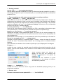
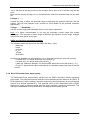
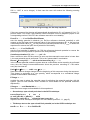
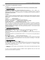
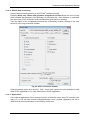
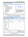
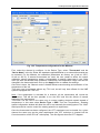
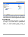
Graph tool: Process data to Generate cycles
Since version 9.20 of EC-Lab® software it is no necessary to process the data file to generate
the cycle number anymore. Now the software is autonomous to generate the cycle number
by itself. For data files recorded before with older versions, the user must process the file to
generate the cycle number.
Note: the automatic cycle number generation is available only with the CV and the CVA
techniques.
Let’s consider a data file made with an old software version. If the CV experiment is made of
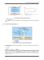
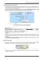
several cycles, the user can highlight the desired cycles. The way to do that is:
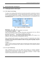
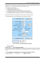
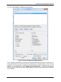
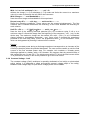
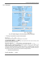
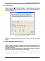
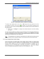
1) In the main menu bar, click on "Analysis / General Electrochemistry / Process
data". The following window appears:
9
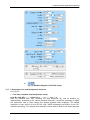
Techniques and Applications Manual
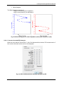
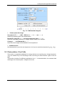
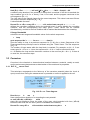
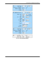
Fig. 5: Cyclic Voltammetry process window.
2) Select on the variables to process.
3) The process is finished when DONE appears.
4) Click on “Display” to plot the processed file
“n” has been added to the name of the processed file as an extension for the cycle number.
The other variables that can be processed in a CV experiment are the charge exchanged
during the oxidation step (Q charge) and during the reduction step (Q discharge) and the
total charge exchanged since the beginning of the experiment (Q-Q0).
10
Techniques and Applications Manual
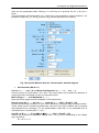
2.1.3 CVA: Cyclic Voltammetry Advanced
The Cyclic Voltammetry Advanced (CVA) is an advanced version of the standard CV
technique (report to the CV description part for more details about the technique). This
technique has been implemented to offer the user all the extended capabilities that can be
required during a potential sweep. In particular, a table has been added to the CVA to link
potential sweeps with different scan rates. A vertex delay is possible at the beginning
potential, at both vertex potentials and the final potential. For each of these delays, the
current and the potential can be recorded at the user’s convenience. A recording condition
on cycles offers the possibility to not store every cycle. A reverse button can be used to
reverse the potential sweep when necessary without modifying the vertex potentials (different
from the Force button).
The technique is composed of:
 starting potential setting block,
 1st potential sweep with a vertex limit E1,
 2nd potential sweep in the opposite direction with a vertex limit E2,
 possibility to repeat nc times the 1st and the 2nd potential sweeps,
 final conditional scan in the reverse direction to the previous one, with its own limit EF.
Note that all the different sweeps have the same scan rate (absolute value). But it is possible
to add sequences allowing to use different rates for each sequence.
The detailed diagram (the following figure) is made of three blocks:
11
Techniques and Applications Manual
Fig. 6: Cyclic Voltammetry Advanced detailed diagram.
 Starting potential:
Set Ewe to Ei = …….. V vs Ref/Eoc/Ectrl/Emeas
sets the starting potential in absolute (vs. Ref the reference electrode potential in the cell) or
according to the previous open circuit potential (Eoc) or controlled potential (Ectrl) or Measured
potential (Emeas).
Hold Ei for ti = ….. h ….. mn ….. s and record every dti = ….. s
offers the possibility to hold the initial potential for a given time and record data points during
this holding period.
12
Techniques and Applications Manual
Note: This function can correspond to a preconditioning capability in an anodic stripping
voltammetry experiment.
 First potential sweep with measurement and data recording conditions:
Scan Ewe with dE/dt = ……. mV/s
allows the user to set the scan rate in mV/s The potential step height and its duration are
optimized by the software in order to be as close as possible to an analogic scan. Between
brackets the potential step height and the duration are displayed according to the potential
resolution defined on the top of the window (in the “Advanced” tool bar).
to vertex potential E1 = ……. V vs Ref/Eoc/Ei.
fixes the first vertex potential value in absolute (Vs. Ref) or according to the previous open
circuit potential (Eoc), or according to the potential of the previous experiment (Ei).
Hold E1 for t1 = ….. h ….. mn ….. s and record every dt1 = ….. s
offers the ability to hold the first vertex potential for a given time and record data points
during this holding period.
Measure <I> over the last ……. % of the step duration
selects the end part of the potential step (from 1 to 100%) for the current average (<I>)
calculation, to possibly exclude the first points where the current may be disturbed by the
step establishment.
Note that the current average (<I>) is recorded at the end of the potential step into the data
file.
Record <I> averaged over N = ……. voltage step(s)
averages N current values on N potential steps, in order to reduce the data file size and
smooth the trace. The potential step between two recording points is indicated between
brackets.
Once selected, an estimation of the number of points per cycle is displayed into the diagram.
E Range = …….
enables the user to select the potential range for adjusting the potential resolution with his
system. (See EC-Lab software user’s manual for more details on the potential resolution
adjustment)
I Range = ……. bandwidth = …… .
enables the user to select the current range and the bandwidth (damping factor) of the
potentiostat regulation.
 Reverse scan:
Reverse scan towards vertex potential E2 = …….. V vs Ref/Eoc/Ei.
runs the reverse sweep towards a 2nd limit potential. The vertex potential value can be set in
absolute (vs. Ref) or according to the previous open circuit potential (Eoc) or according to the
potential of the previous experiment (Ei).
Hold E2 for t2 = ….. h ….. mn ….. s and record every dt2 = ….. s
offers the ability to hold the second vertex potential for a given time and to record data points
during this holding period.
 Repeat option for cycling:
Repeat nc = …….. times
13
Techniques and Applications Manual
repeats the whole sequence nc time(s). Note that the number of repeat does not count the
first sequence: if nc = 0 then the sequence will be done 1 time, nc = 1 the sequence will be
done 2 times, nc = 2, the sequence will be 3 times...
Record the first cycle and every nr = ….. cycle(s)
offers the ability for the user to store only one cycle every n r cycle in case of many cycles in
the experiment. The first cycle is always stored.
 Final potential:
Reverse scan (yes or no) towards EF = ……… V vs Ref/Eoc/Ei.
gives the ability to end the potential sweep or to run a final sweep with a limit EF.
Hold Ef for tf = ….. h ….. mn ….. s and record every dtf = ….. s
offers the possibility to hold the final potential for a given time and record data points during
this holding period.
Options:
1- Reverse
While the experiment is running, clicking on this button allows the user to reverse the
potential scan direction instantaneously. Contrary to the Force button, the vertex potential is
not replaced by the current potential value. E1 and E2 are kept.
2- Force E1 / E2
While the experiment is running, clicking on this button allows the user to stop the potential
scan, set the instantaneous running potential value Ewe to E1 or E2 (according to the scan
direction), and start the reverse scan. Thus E1 or (and) E2 are modified and adjusted in order
to reduce the potential range.
Clicking on this button is equivalent to click on the "Modify" button. Enter the running
potential as E1 or E2 and validate the changed parameters with the accept button. This button
enables the user to perform the operation faster when the limit potentials have not been
properly estimated and continue the scan without damaging the cell.
Note: it is highly recommended that the user adjusts the potential resolution (from 300 µV for
20 V amplitude to 5 µV for 0.2 V amplitude with a SP-150, VSP or VMP3) according to the
experiment potential limit. This will considerably reduce the noise level and increase the plot
quality.
3- Hold E
While the experiment is running, clicking in this button allows the user to hold the actual
potential. Clicking again on this button the experiment will continue in the same direction.
4- Table/Sequence
The CVA technique is equipped with a table, the ability to add sequences. This allows the
user to link several sequences of CVA with different scan rates or different vertex potentials.
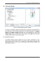
Graph tool: Process Data
When the CVA experiment is made, the user can extract the charge quantities exchanged
during the anodic step (Q charge), the cathodic step (Q discharge), and the total charge
exchanged since the beginning of the experiment (Q-Q0).
14
Techniques and Applications Manual
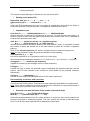
2.1.4 Linear Sweep Voltammetry: LSV
The linear sweep voltammetry technique is a standard electrochemical protocol. Unlike the
CV, no backward scan is done, only the forward scan is applied. This technique is specially
dedicated to RDE (Rotating Disk Electrode) or RRDE (Rotating Ring Disk Electrode)
investigations which allows user to carry out steady-state measurements. This leads to the
determination of redox potential and kinetic parameters. The “External Device Configuration”
of EC-Lab menu makes easy to control and measure the rotating rate of the R(R)DE device.
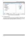
Fig. 7: Linear Sweep Voltammetry detailed diagram.
 Rest period
Rest for tR =
h
mn
s
fixes a defined time duration tR for recording the rest potential.
or until |dEwe/dt| < |dER/dt| =
mV/h
stops the rest sequence when the slope of the open circuit potential with time, |dER/dt|
becomes lower than the set value (value 0 invalidates the condition).
Record Ewe every dER =
mV or dtR =
s
allows the user to record the working electrode potential whenever the change in the
potential is  dER with a minimum recording period in time dtR.
 Potential sweep with measurement and data recording conditions:
Scan Ewe with dE/dt = ……. mV/s
allows the user to set the scan rate in mV/s The potential step height and its duration are
optimized by the software in order to be as close as possible to an analogic scan. Between
15
Techniques and Applications Manual
brackets the potential step height and the duration are displayed according to the potential
resolution defined on the top of the window (in the “Advanced” tool bar).
From Ei = ......V vs. Ref/Eoc/Ei.
fixes the intial potential value in absolute (Vs. Ref) or according to the previous open circuit
potential (Eoc), or according to the potential of the previous experiment (Ei).
to EL = ……. V vs Ref/Eoc/Ei.
fixes the limit potential value in absolute (Vs. Ref) or according to the previous open circuit
potential (Eoc), or according to the potential of the previous experiment (Ei).
Hold E1 for t1 = ….. h ….. mn ….. s and record every dt1 = ….. s
offers the ability to hold the first vertex potential for a given time and record data points
during this holding period.
Record <I> over the last ……. % of the step duration
selects the end part of the potential step (from 1 to 100%) for the current average (<I>)
calculation, to possibly exclude the first points where the current may be disturbed by the
step establishment.
Note that the current average (<I>) is recorded at the end of the potential step into the data
file.
averaged over N = ……. voltage step(s)
averages N current values on N potential steps, in order to reduce the data file size and
smooth the trace. The potential step between two recording points is indicated between
brackets.
Once selected, an estimation of the number of points per cycle is displayed into the diagram.
E Range = …….
enables the user to select the potential range for adjusting the potential resolution with his
system. (See EC-Lab software user’s manual for more details on the potential resolution
adjustment)
I Range = ……. bandwidth = …… .
enables the user to select the current range and the bandwidth (damping factor) of the
potentiostat regulation.
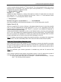
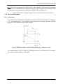
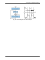
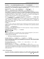
2.1.5 Chrono I/Q: Chronoamperometry / Chronocoulometry
The basis of the controlled-potential techniques is the measurement of the current response
to an applied potential step.
Chronoamperometry involves stepping the potential of the working electrode from an initial
potential, at which no faradic reaction generally occurs, to a potential Ei at which no
electroactive species exist (at the beginning of the experiment). The current-time response
reflects the change in the concentration gradient in the vicinity of the surface.
Chronoamperometry is often used for measuring the diffusion coefficient of electroactive
species or the surface area of the working electrode. This technique can also be applied to
the study of electrode processes mechanisms.
An alternative and very useful mode for recording the electrochemical response is to
integrate the current, so that one obtains the charge passed as a function of time. This is the
chronocoulometric mode that is particularly used for measuring the quantity of adsorbed
reactants.
The potential steps can be set to a fixed value (Ei) or relatively to the last rest potential (E<oc>)
or the last controlled potential (Epc).
16
Techniques and Applications Manual
Fig. 8: Chronoamperometry / Chronocoulometry general diagram.
The detailed diagram is composed of two blocks:
 potential step,
 loop.
17
Techniques and Applications Manual
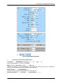
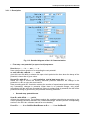
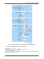
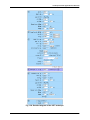
Fig. 9: Chronoamperometry / Chronocoulometry detailed diagram and table.

Potential step with data recording conditions:
1) Potential step
Apply Ei = ………… V vs Ref/Eoc/Ectrl/Emeas.
the potential step is defined in absolute (vs. Ref the reference electrode potential) or
according to the previous open circuit potential (Eoc), controlled potential (Ectrl) or measured
potential (Emeas).
for ti = ……….. h ……… mn …….. s
fixes the potential step duration.
limit |I| to IMax = ….. pA/…/A
and |Q| < QM =
fA.h/…/A.h/pC/…/kC.
Imin = …… pA/…/A
curtails the step duration if the current or charge limit is reached. If the limit is reached, the
loop condition (go to Ns' for nc times), if set, is not used, and the program continues to the
next sequence (Ns + 1).
The |Q| value is the integral charge for the current sequence. This value is not reset if there
is a loop on the same sequence (Ns' = Ns).
0 values disable the tests.
2) Recording conditions
Record I every dIp = …. pA/…/A, dQp = …… fA.h/…/A.h/pC/…/kC and dtp = …. S
<I> every dts = …….. s
18
Techniques and Applications Manual
you can record either an instantaneous current value I or an averaged current value <I>. The
recording conditions during the potential step depend on the chosen current variable. For the
instantaneous current the recording values can be entered simultaneously. Then it is the first
condition reached that determines the recording. A zero value disables the recording for
each criterion. For the averaged current the user defines the time for the average calculation.
In that case the data points are recorded in the channel board memory every 200 µs for the
VMP2, VMP3, VSP, SP-150, SP-50, BiStat and the SP-300, SP-200, HCPs and CLB-500
and 20 ms for the VMP and the MPG.
Leave dI alone for Chronoamperometry experiments, and dQ for Chronocoulometry
experiments.
E Range = …….
enables the user to select the potential range for adjusting the potential resolution with his
system. (See EC-Lab software user’s manual for more details on the potential resolution
adjustment)
I range = ……. bandwidth = …… .
enables the user to select the current range and the bandwidth (damping factor) of the
potentiostat regulation.

Loop
goto Ns' =
for nc =
time(s)
allows the experiment to loop to a previous line Ns' (<= Ns) for nc times. The number of loops
starts while the loop block is reached. For example, on Ns = 3, if one enters goto Ns' = 2 for
nc = 1 time, the sequence Ns = 2, Ns = 3 will be executed 2 times.
nc = 0 disables the loop and the execution continue to the next line (Ns' = Ns + 1). If there is
no next line, the execution stops.
Report to the battery techniques section (3.1, page 83) for more details on loop conditions.
Here, it is possible to loop to the first instruction (Ns = 0) and the current instruction (Ns’ = Ns).
This is different from battery experiments (GCPL and PCGA) where the first instruction has a
special meaning and there is still a loop on the current instruction.
This
technique
uses
a
sequence
table.
Sequences
of
the
Chronoamperometry / Chronocoulometry technique can be chained using the "Table" frame.
The first sequence is Ns = 0. Each line of the table (Ns) corresponds to a rest and potential
step sequence. The sequences lines are executed one after the other, and it is possible to
loop to a previous sequence line (Ns’).
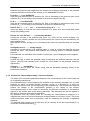
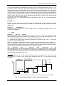
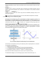
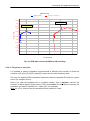
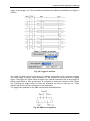
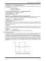
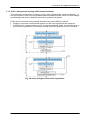
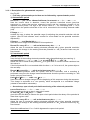
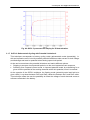
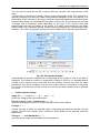
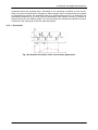
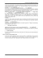
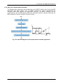
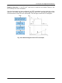
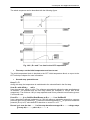
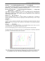
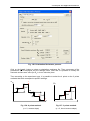
Example: Setting Ei = Eoc + Ei0 on the first sequence (Ns = 0) and Ei = Epc + Ei1 on the next
sequence (Ns = 1), with a loop on the same sequence (goto Ns' = 1), will perform the next
recording:
N s=1, loop 0
N s=0
N s=1, loop 1 N s=1, loop 2
E
E + E
E + E
E + E
E + E
E
E
E
oc
E
oc
oc
oc
t
Fig. 10: Chronoamperometry / Chronocoulometry example.
19
Techniques and Applications Manual
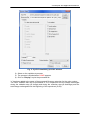
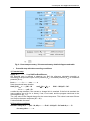
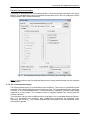
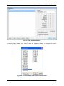
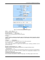
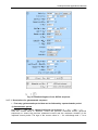
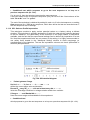
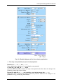
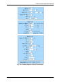
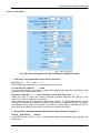
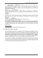
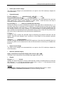
Process: chronocoulometry
A process is associated with chronoamperometry / chronocoulometry technique (see figure
below). The variables that can be processed are the same as for the CV technique and the
charge variation dQ (chronocoulometry).
Fig. 11: Chronoamperometry/chronocoulometry processing window.
Note: In this technique the first and last data points of each potential steps are not recorded
automatically.
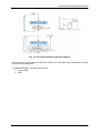
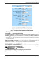
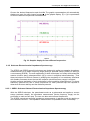
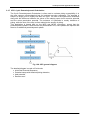
2.1.6 CP: Chronopotentiometry
The Chronopotentiometry is a controlled current technique. The current is controlled and the
potential is the variable determined as a function of time. The chronopotentiometry technique
is similar to the Chronoamperometry / Chronocoulometry technique, potential steps being
replaced by current steps. The constant current is applied between the working and the
counter electrode.
This technique can be used for different kinds of analysis or to investigate electrode kinetics.
But, it is considered less sensitive than voltammetric techniques for analytical uses.
Generally, the curves Ewe = f(t) contain plateaus that correspond to the redox potential of the
electroactive species.
20
Techniques and Applications Manual
Fig. 12: Chronopotentiometry general diagram.
This technique uses a sequence table also. Each line of the table (Ns) corresponds to a rest
and current step sequence.
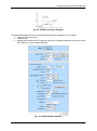
The detailed diagram is made of two blocks:
 current step,
 loop.
21
Techniques and Applications Manual
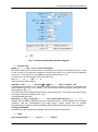
Fig. 13: Chronopotentiometry detailed diagram.

Current step
Apply Is = ………. pA/…/A vs. <none>/Ictrl/Imeas.
the current step is set to a fixed value or relatively to the previous controlled current I ctrl, that
is the current of the previous sequence current step block or to the previous measured
current Imeas. This option is not available on the first sequence (Ns = 0).
To select the current step type, check the option box.
for ts = ……… h ……… mn ……… s
fixes the current step duration.
limit |Ewe| < EM = ………….. mV and |Q| < QM = ………. fA.h/…/A.h/pC/…/kC
curtails the step duration if the potential or charge limit is reached. If the limit is reached, the
loop condition (go to Ns' for nc times), if set, is not used, and the program continues to the
next sequence (Ns + 1).
The |Q| value is the integral charge for the current sequence. This value is not reset if there
is a loop on the same sequence (Ns' = Ns).
0 values disable the tests.
Record Ewe or <Ewe> every dEs = ………… mV, and at least every dts = ………….. s
defines the recording conditions during the potential step. 0 values disable the recording
condition, and the corresponding box stays green. These values can be entered
simultaneously, and this is the first condition that is reached that determines the recording.
I Range, Bandwidth
selects the current range and bandwidth values for the whole sequences.

Loop
goto sequence Ns' = ………. for nc = ………… time(s)
22
Techniques and Applications Manual
gives the ability to loop to a previous sequence Ns' (<= Ns) for nc times. Sequences of the
chronopotentiometry technique can be chained using the "Table" frame. The first sequence
is Ns = 0.
The number of loops starts while the loop block is reached. For example, on Ns = 3, if one
enters goto Ns' = 2 for nc = 1 time, the sequence Ns = 2, Ns = 3 will be executed 2 times.
nc = 0 disables the loop and the execution continue to the next line (Ns' = Ns + 1). If there is
no next line, the execution stops.
Report to the battery techniques section (3.1, page 83) for more details on loop conditions.
Thus, it is possible to loop to the first instruction (Ns = 0) and the current instruction (Ns’ = Ns).
That is different from the battery experiments (GCPL and PCGA) where the first instruction
has a special meaning and where there is still a loop on the current instruction.
Process:
A process function is associated with chronopotentiometry technique. The variables that can
be processed are the same as for the CV technique. For more details about CP process see
the previous CV part.
Note: In this technique the first and last data points of each current steps are not recorded
automatically.
2.1.7 SV: Staircase Voltammetry
Staircase voltammetry (SV) is one of the most widely used techniques for acquiring
qualitative information about electrochemical reactions. SV like cyclic voltammetry provides
information on redox processes, heterogeneous electron-transfer reactions and adsorption
processes. It offers a rapid location of redox potential of the electroactive species.
SV consists of linearly scanning the potential of a stationary working electrode using a
triangular potential waveform with a potential step amplitude and duration defined by the
user. During the potential sweep, the potentiostat measures the current resulting from
electrochemical reactions (consecutive to the applied potential). The cyclic voltammogram is
a current response as a function of the applied potential.
Contrary to the cyclic voltammetry, the potential steps are not as small as possible but
adjusted exactly to the user’s convenience.
Fig. 14: General diagram for Staircase Voltammetry.
23
Techniques and Applications Manual
This technique is similar to the usual cyclic voltammetry, but using significant digital potential
staircase (i.e. it runs defined potential increment regular in time).
The technique is composed of:
 a starting potential setting block,
 a 1st potential sweep with a final limit E1,
 a 2nd potential sweep in the opposite direction with a final limit E2,
 the possibility to repeat nc times the 1st and the 2nd potential sweeps,
 a final conditional scan reverse to the previous one, with its own limit EF.
Note that all the different sweeps have the same scan rate (absolute value).
The detailed diagram (on the following figure) is made of three blocks:
Fig. 15: Staircase Voltammetry detailed diagram.

Starting potential:
Set Ewe to Ei = …….. V vs Ref/Eoc/Ectrl/Emeas
sets the starting potential in absolute (vs. Ref the reference electrode potential) or according
to the previous open circuit potential (Eoc), controlled potential (Ectrl) or measured potential
(Emeas).

First potential sweep with measurement and data recording conditions:
Scan Ewe with dE = ……. mV per dt = ……….. s ( 300 µV/15 ms)
24
Techniques and Applications Manual
allows the user to set the potential step height in mV and the step duration in s. Between
brackets the scan rate is displayed according to the potential resolution defined by the user
in the “Advanced Settings” window (see the corresponding section in the EC-Lab® software
manual for more details).
to vertex potential E1 = ……. V vs Ref/Eoc/Ei.
fixes the first vertex potential value in absolute (vs. Ref the reference electrode potential) or
according to the previous open circuit potential (Eoc), or to the initial potential (Ei).

Reverse scan
Reverse scan towards vertex potential E2 = …….. V vs Ref/Eoc/Ei.
runs the reverse sweep towards a 2nd limit potential. The vertex potential value can be set in
absolute (vs. Ref the reference electrode potential) or according to the previous open circuit
potential (Eoc) or to the initial potential (Ei).

Repeat option for cycling
Repeat nc = …….. times
repeats the whole sequence nc time(s). Note that the number of repeat does not count the
first sequence: if nc = 0 then the sequence will be done 1 time, nc = 1 the sequence will be
done 2 times, nc = 2, the sequence will be 3 times...
Measure <I> over the last ……. % of the step duration
selects the end part of the potential step (from 1 to 100%) for the current average (<I>)
calculation, to possibly exclude the first points where the current may be disturbed by the
step establishment.
Note that the current average (<I>) is recorded at the end of the potential step in the data file.
Record <I> averaged over N = ……. voltage step(s)
averages N current values on N potential steps, in order to reduce the data file size and
smooth the trace. The potential step between two recording points is indicated between
brackets.
Once selected, an estimation of the number of points per cycle is displayed in the diagram.
E Range = …….
enables the user to select the potential range for adjusting the potential resolution with his
system. (See EC-Lab software user’s manual for more details on the potential resolution
adjustment)
I range = ……. bandwidth = …… .
enables the user to select the current range and the bandwidth (damping factor) of the
potentiostat regulation.

Final potential
Reverse scan (yes or no) towards EF = ……… V vs Ref/Eoc/Ei.
give the possibility to end the potential sweep or to run a final sweep with a limit EF.
Option: Force E1 / E2
While the experiment is running, clicking on this button allows the user to stop the potential
scan, set the instantaneous running potential Ewe to E1 or E2 (according to the scan
direction), and start the reverse scan. Thus EL1 and/or EL2 are modified and adjusted in order
to reduce the potential range.
Clicking on this button is equivalent to click on the "Modify" button. Enter the running
potential as E1 or E2 and validate the changed parameters with the accept button. This button
25
Techniques and Applications Manual
allows the user to perform the operation faster when the limit potentials have not been
properly estimated and to continue the scan without damage to the cell.
Note: it is highly recommended to adjust the potential resolution according to the experiment
potential limit. This will considerably reduce the noise level and increase the plot quality.
Graph tool: Generate cycles
See the cyclic voltammetry technique for more details.
2.1.8 LASV: Large Amplitude Sinusoidal Voltammetry
Large Amplitude Sinusoidal Voltammetry (LASV) is an electrochemical technique where the
potential excitation of the working electrode is a large amplitude sinusoidal waveform. Similar
to the cyclic voltammetry (CV) technique, it gives qualitative and quantitative information on
the redox processes. In contrast to the CV, the double layer capacitive current is not subject
to sharp transitionsat reverse potentials. As the electrochemical systems are non-linear the
current response exhibits higher order harmonics at large sinusoidal amplitudes. Valuable
information can be found from data analysis in the frequency domain.
Fig. 16: General diagram for Large Amplitude Sinusoidal Voltammetry.
This technique is similar to usual cyclic voltammetry, but using a frequency to define the scan
speed. The curve of the potential excitation can be compared to a large amplitude sinusoidal
waveform.
The technique is composed of:
 a starting potential setting block,
 a frequency definition fs,
 a potential range definition from E1 to E2,
 the possibility to repeat nc times potential scan.
The detailed diagram (on the following figure) is made of two blocks:
26
Techniques and Applications Manual
Fig. 17: Staircase Voltammetry detailed diagram.

Starting potential:
Set Ewe to Ei = …….. V vs Ref/Eoc/Ectrl/Emeas
sets the starting potential in absolute (vs. Ref the reference electrode potential) or according
to the previous open circuit potential (Eoc) or controlled potential (Ectrl) or Measured potential
(Emeas).

Frequency and Potential range definition with measurement and data recording
conditions:
Apply a sinusoidal potential scan
With frequency fs = ….. kHz/Hz/mHz/µHz
Allows the user to set the value of frequency which will define the scan rate.
Between vertex potential E1 = ….. V vs Ref/Eoc/Ei
Fixes the first vertex potential value in absolute (vs. Ref the reference electrode potential) or
according to the previous open circuit potential (Eoc) or previous potential (Ei).
And vertex E2 = …V vs vs Ref/Eoc/Ei
Fixes the second vertex potential value in absolute (vs. Ref the reference electrode potential)
or according to the previous open circuit potential (Eoc) or previous potential (Ei).
Repeat nc = …….. times
repeats the whole sequence nc time(s). Note that the number of repeat does not count the
first sequence: if nc = 0 then the sequence will be done 1 time, nc = 1 the sequence will be
done 2 times, nc = 2, the sequence will be 3 times...
Record every dt = ….. s and dI = ….. nA/µA/mA/A
27
Techniques and Applications Manual
offers the possibility to record I with two conditions on the current variation dI and (or) on time
variation.
E Range = …….
enables the user to select the potential range for adjusting the potential resolution with his
system. (See EC-Lab software user’s manual for more details on the potential resolution
adjustment)
I range = ……. bandwidth = …… .
enables the user to select the current range and the bandwidth (damping factor) of the
potentiostat regulation.
Note: this technique includes sequences to link sines with different amplitude for example.
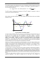
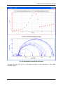
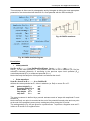
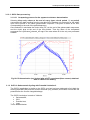
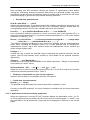
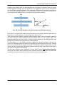
2.1.9 Alternating Current Voltammetry (ACV)
Alternating Current Voltammetry (ACV) is assimilated to a faradaic impedance technique. On
this technique a sinusoidal voltage of small amplitude (A) with a constant frequency (f s) is
superimposed on a linear ramp between two vertex potentials (E1, E2). The potential sweep
is defined as follow E (t )  E1,2 
dE
t  A sin(2. .fs .t ) . Typically, the linear ramp varies on a
dt
long time scale compared to the superimposed AC variation.
Like the pulsed techniques, ACV discriminates the faradaic current from the capacitive one.
Consequently, ACV can be used for analytical purpose. Moreover this technique can also be
used for investigating electrochemical mechanism, for instance superimposition of forward
and backward scan characterize a reversible redox system.
Fig. 18: General diagram for Alternating Current Voltammetry.
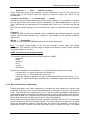
This technique corresponds to usual cyclic voltammetry with a superimposition of a sinusoid.
The technique is composed of:
 a starting potential setting block,
 a 1st potential sweep with a final limit E1 and a sinusoid superimposed,
 a 2nd potential sweep in the opposite direction with a final limit E2 (option),
 the possibility to repeat nc times the 1st and the 2nd potential sweeps.
Note that all the different sweeps have the same scan rate (absolute value).
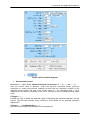
The detailed flow diagram (on the following figure) is made of three blocks (Fig. 17):
28
Techniques and Applications Manual
Fig. 19: Alternating Current Voltammetry detailed diagram.
 Starting potential
Set Ewe to Ei = …….. V vs Ref/Eoc/Ectrl/Emeas
sets the starting potential in absolute (vs. Ref, the reference electrode potential in the cell) or
according to the previous open circuit potential (Eoc) or controlled potential (Ectrl) or Measured
potential (Emeas).
 Potential sweep with superimposition of sinusoid signal and measurement and data
recording conditions
Scan Ewe with dE/dt = ……. mV/s
allows the user to set the scan rate in mV/s The potential step height and its duration are
optimized by the software in order to be as close as possible from an analogic scan.
to vertex potential E1 = ……. V vs Ref/Eoc/Ei
fixes the first vertex potential value in absolute (vs. Ref) or according to the previous open
circuit potential (Eoc) or previous potential (Ei).
Add a sinusoidal signal to the potential scan
With frequency fs = …….. kHz/Hz/mHz/µHz
And amplitude A = … mV
defines the properties (frequency and amplitude) of the sinusoidal signal.
[] Reverse scan to vertex E2 = … V vs Ref/Eoc/Ei
29
Techniques and Applications Manual
offers the possibility to do a reverse scan and to fixe the value of the vertex potential value in
absolute (vs. Ref) or according to the previous open circuit potential (Eoc) or previous
potential (Ei).
Repeat nc = …….. times
repeats the whole sequence nc time(s). Note that the number of repeat does not count the
first sequence: if nc = 0 then the sequence will be done 1 time, nc = 1 the sequence will be
done 2 times, nc = 2, the sequence will be 3 times...
E Range = …….
enables the user to select the potential range for adjusting the potential resolution with his
system. (See EC-Lab software user’s manual for more details on the potential resolution
adjustment)
I range = ……. bandwidth = …… .
enables the user to select the current range and the bandwidth (damping factor) of the
potentiostat regulation.
Reverse scan towards Ei
offers the possibility to do a reverse scan towards Ei.
2.2 Electrochemical Impedance Spectroscopy
Methods employing excitation of an electrochemical cell by a sinusoidal signal were first
employed as a way of measuring the rate constant of fast electron transfer reactions at short
times. Now the interest rests on the complete analysis of what are often complicated
processes involving surface and solution reactions (electrode and electrolyte). Among the
modern computational techniques, the Electrochemical Impedance spectroscopy (EIS) is
now a powerful tool for examining many chemical and physical processes in solution as well
as in solids. EIS has uses in corrosion, battery, fuel cell development, sensors and physical
electrochemistry and can provide information on reaction parameters, corrosion rates,
electrode surfaces porosity, coating, mass transport, and interfacial capacitance
measurements.
The VMP2/Z / VMP3 / VSP / SP-150 boards are designed to perform impedance
measurements independently or simultaneously, from 10 µHz to 1 MHz (200 kHz for channel
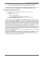
boards delivered before July 2005). For SP-300 and SP-200, the maximum frequency is
7 MHz.
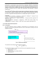
Since the EC-Lab® version 9.50, a multisinus measurement was introduced for the
impedance measurement techniques.
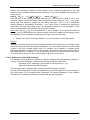
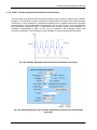
2.2.1 Principles of multisine measurements
To spare time during impedance measurements especially in low frequencies range but also
to avoid the measurement drifts - if the system changes quickly with time - it may be useful to
use a multisine excitation signal.
Indeed, to get information at different frequencies with an excitation signal, the system has to
be excited successively by one frequency at the time, resulting in a very long experiment.
Indeed, the total time taken for the complete analysis is the sum of the individual
measurement times. This is the case for the single sine measurement.
In multisine measurement, all the frequencies are analyzed at the same time. Then, the use
of Schroeder multisine, simultaneous application of several sinewave, allows the user to
save a lot of time, especially for measurement at low frequency.
30
Techniques and Applications Manual
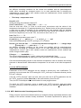
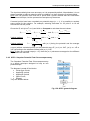
The multisine signal is thus defined as the sum of sinusoids at different frequencies having
the same programmable amplitudes A - resulting in a time signal - and different phases  ,
with the following formula [1]:
N
k1
(k  n)
[1].
N
n1
u(t)  A cos(2f k t  k ) with the phase k  1  2
k1
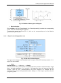
The EIS multisine measurement developed in EC-Lab® software is defined in order to
minimize the crest factor defined by:


Cr(u ) 
uM  um
with
2u eff
ueff  A
N
[2]
2
With multisine calculation defined in EC-Lab® software, the crest factor values are included
between 2 and 3.

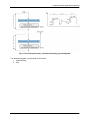
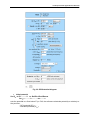
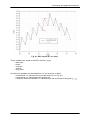
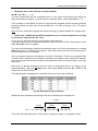
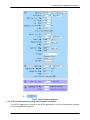
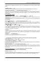
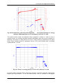
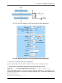
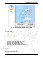
Fig. 20: Scheme of multisine signal.
To avoid a large excitation at the sine origin that could damage the electrochemical cell, all
the sine are out of phase the ones compared to the others. Indeed, in multisine
measurement a multiplicative factor can be applied on the signal amplitude – which can
reach UM or Um values. Generally, it is better to not exceed 50 mV of sinus amplitude.
Indeed, if the excitation – which is the sum of the maximum amplitude of all the applied
frequencies – is too large, this might result in a measurement in the non-linear response
domain of the electrochemical cell. Then, the sine amplitude values need to be minimized
and accordingly the non-linear response of the system is minimized.
Obviously, the number of frequencies summed depends on the user needs, defined in the
settings of the electrochemical impedance spectroscopy technique. In EC-Lab® software,
multisine measurement is done simultaneously on a maximum of two decades. If the
experiment is defined with more than two decades of twenty sine, the cutting out is
automatically done by set of twenty sine.
To avoid noisier or non-linear results user has to define carefully the experimental conditions.
An appropriate level of excitation has to be defined. Indeed, since a lot of frequencies are
stimulated in the same time, there is less signal level at each frequency and then impedance
measurement results tend to be noisier. However, increasing the level of excitation can bring
to do impedance measurements in a non-linear condition and then impedance results are not
good.
To define the right excitation conditions, the user has to know that in EC-Lab® software, the
maximum amplitude of the signal is defined as 0.5 V and half of the I Range, for
31
Techniques and Applications Manual
potentiostatic or galvanostatic mode measurement, respectively. Multisine measurements
are done only for frequencies smaller that 1 Hz, in the remainder of the frequency range only
single sine measurement is available. Note that if the frequency range defined by the user is
included in the two kinds of measurement (single sine and multisine), the measurement will
be done in continuity with first a single sine measurement and afterwards a multisine
measurement.
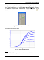
Then with EC-Lab® software, multisine measurements are faster than single sine ones (by an
order of 3), that is very interesting for systems with a rapid change. Nevertheless, definition
of measurement conditions, especially value of the excitation of the electrochemical cell, has
to be done in agreement with the preservation of a steady-state regime of the system.
References:
- Van Gheem E., Vereecken J., Schoukens J., Pintelon R., Guillaume P., Verboven P. and
Pauwels L., Electrochim. Acta 49 (2004) 2919-2925.
- Pintelon R. and Schoukens J., System identification – A frequency Domain approach, Ed.
IEEE Press, 2001.
- Van der Ouderaa E., Schoukens J., Renneboog J., IEEE Trans. Instrum. Meas. 37(1)
(1988) 145-147.
- Schoeder M. R., Pintelon R., Rolain Y., IEEE Trans. Instrum. Meas. IM-49 (2000) 275.
2.2.2 PEIS: Potentiostatic Impedance
2.2.2.1 Description
The PEIS experiment performs impedance measurements into potentiostatic mode by
applying a sinus around a potential E that can be set to a fixed value or relatively to the cell
equilibrium potential.
Fig. 21: PEIS general diagram.
The potential of the working electrode follows the equation:
E
we
 E  V sin(2 π f t)
a
The detailed flow diagram is made of four blocks that can be separated into four parts:
 single or multi sine mode,
 initial potential,
 frequency scan with recording conditions,
 repeat sequence.
32
Techniques and Applications Manual
Fig. 22: PEIS detailed diagram.

Initial potential
Set Ewe to E = …….. V vs. Ref/Eoc/Ectrl/Emeas
for tE = ……… h ………. mn …… s
sets the potential to a fixed value E (vs. Ref, the reference electrode potential) or relatively to
the previous:
- OCV potential (Eoc),
- controlled potential (Ectrl),
33
Techniques and Applications Manual
- measured potential (Emeas),
for a tE duration. Sets tE large enough to wait for the cell current stabilization, if the applied
potential is different from the open circuit potential. During this period, no impedance
measurement is done.
Note: if another experiment is defined before, then it is possible to define the initial potential
as a function of Ectrl and Emeas (previous potential controlled and previous potential measured,
respectively). If there is no experiment before it is not possible to use Ectrl and Emeas.
Record every dI = ….. nA/µA/mA/A and dt = ….. s
offers the possibility to record Ewe and I during the DC period before the AC simulation with
two conditions on the current variation dI and (or) on time variation.

Impedance scan
Scan from fi = ……… MHz/kHz/Hz/mHz/µHz to ff = ……… MHz/kHz/Hz/mHz/µHz
defines the initial (fi) and final (ff) frequencies of the scan. To have the first measured point
more rapidly, it is recommended to scan from the highest frequencies to the lowest ones, but
it is possible to reverse the frequencies scan order.
with Nd = ……… points per decade
in
Logarithm spacing
Nt = ……… points from fi to ff in Linear spacing
defines the frequencies distribution between the scan bounds f i and ff. It is possible to select
the number of points per decade Nd or the total number of points Nt, in linear or logarithm
spacing.
For example, a scan from fi = 100 kHz to ff = 1 kHz with Nd = 5 points per decade in logarithm
spacing, will perform measures at the following frequencies (in kHz):
100, 63.1, 39.8, 25.1, 15.8, 10, 6.31, 3.98, 2.51, 1.58, 1
and a scan from fi = 100 kHz to ff = 1 kHz with Nt = 11 total number of points in linear
spacing, will make measures at these following frequencies (Hz):
100, 90, 80, 70, 60, 50, 40, 30, 20, 10, 1
Click on the Show frequencies >> button to display the list of the scanned frequencies.
Note: it is not possible to select Nd points per decade in linear spacing.
with an amplitude Va = …… mV
sets the sinus amplitude to Va. Equivalence with VRMS is also given.
Note the following relationships between Va, Vpp and VRMS Va = Vpp/2 and VRMS = Vpp/(2 2 ).
Wait for pw = …… period before each frequency measurement
offers the possibility to add a delay before the measurement at each frequency. This delay is
defined as a part of the period. Of course for low frequencies the delay may be long.
average Na = ……… mesure(s) per frequency
repeats Na measure(s) and average the values for each frequency.
Non stationary correction: drift correction
corrects the drift of the system. This feature is more specially dedicated to low frequencies.
Note:
1- If this option is selected, the sinus frequencies are evaluated over 2 periods (instead
of 1), increasing the acquisition time by a factor of 2.
2- In the bottom right corner of the block, the approximate experiment duration is
indicated as information for the user.
During the Run, several parameters remain accessible for modification such as the min and
max frequencies and the number of points per decade.
34
Techniques and Applications Manual

Repeat
Repeat for nc = ……… time(s)
allows for repeating PEIS measurements in order to represent Z evolution vs. time (see
below).
E Range = …….
enables the user to select the potential range for adjusting the potential resolution with his
system. (See EC-Lab software user’s manual for more details on the potential resolution
adjustment)
I Range = ………. Bandwidth = …….
Sets the current range and bandwidth values for the whole experiment.
 Sequence repetition
The last part of this technique is dedicated to repeat sequences when many sequences are
done. Indeed since the version 9.9 of EC-Lab® software it is possible to add sequence in
impedance measurements. This tool is convenient to spare time, indeed during the same
experiment it is possible to work in single sine mode at high frequencies and in mutisine
mode at low frequencies or to change the sinus amplitude.
When the box Increment cycle number is ticked, each sequence will be considered as a
cycle. This tool is useful to fit EIS data files with ZFit.
2.2.2.2 Additional features:



It is possible to add sequences. This could be very useful to do a first part of the high
frequencies experiment with single sine measurement and the second part of the
experiment at low frequencies with multisine measurement. This will allow the user to
spare time.
It is possible to modify on-line the settings of an impedance measurement during the
experiment. The user can Modify, Pause, Resume or Stop the experiment while running.
The counter electrode potential can be recorded in EIS techniques. So the EIS
measurement is done simultaneously on the working electrode and on the counter
electrode. To do that, select “Record Ece” in the Cell characteristics tab. Nyquist and
Bode diagrams can be plotted for both the WE and the CE electrodes. The working and
counter electrode variables are displayed respectively as follows with the additional
extension Re (Z) and Re (ZCE), -Im (Z) and –Im (ZCE).
2.2.3 GEIS: Galvanostatic Impedance
This technique is very close to the Potentiostastic Impedance technique (PEIS), except that
the current is controlled instead of the potential. So report to the PEIS experiment section for
more details.
35
Techniques and Applications Manual
Fig. 23: GEIS diagram.
Note that the current can be applied vs. the previous control current or the previous
measured current (previous sequence of a linked technique).
Instead of Ia, one can consider the current peak to peak amplitude (Ipp) related to Ia with
Ipp=2*Ia or the Root Mean Square (RMS) voltage related to Ia with IRMS = Ia/ 2 .
36
Techniques and Applications Manual
2.2.4 Visualisation of impedance data files
2.2.4.1 Standard visualisation modes
EC-Lab® software provides a full range of variables and visualisation modes defined by
default. When an impedance data file is displayed, click on “Selector” to show all the
variables and visualisation modes available with impedance data files:
Fig. 25: Impedance graph plot
selector.
Fig. 24: Impedance data file selector.
Among the available variables the Impedance Z is calculated using Fast Fourier Transform
function and the admittance Y is determined as Y=1/Z. For both variables Bode, Nyquist and
Black diagrams can be plotted according to the EC-Lab® software’s predefined graph
visualization modes.
37
Techniques and Applications Manual

Bode diagram (for both impedance and admittance)
The Bode diagram is the plot of:
-
log|Z| versus log(f) and Z-phase versus
log(f) for the impedance
-
log|Y| versus log(f) and Y-phase versus
log(f) for the admittance.
On the first figure log |Z| and log |Y| have been
overlaid on the same graph. On the second one
Phase(Z) and Phase(Y) have been overlaid.
Fig. 26: BODE diagrams for both
impedance (blue) and admittance (red).

Nyquist diagram
The Nyquist diagram is the plot of:
- –Im(Z) versus Re(Z) for impedance
-
Im(Y) versus Re(Y) for admittance.
The main difference between both visualizations
is that the admittance diagram better shows the
high frequency semi-circle.
With the Nyquist visualization, the axes are
automatically displayed proportionally.
Fig. 27: NYQUIST diagrams for both
impedance (blue) and admittance (red).
38
Techniques and Applications Manual

Black Diagram
The Black diagram is the plot of
- log|Z| versus phase(Z) for impedance
- log|Y| versus phase(Y) for admittance.
Fig. 28: BLACK diagrams for both impedance (blue) and admittance (red).
2.2.4.2 Counter electrode EIS data plot
When the user selects “Record Ece” in the Cell characteristics window, EIS measurement of
the counter electrode is done and can be displayed.
Fig. 29: EIS variable selection window with WE and CE.
39
Techniques and Applications Manual
PEIS contre.m pr
-Im(Z) vs. Re(Z)
-Im(Zce) vs. Re(Zce) #
0,025
Counter electrode
0,02
0,015
Working electrode
- Im ( Z ce) /O h m
0,01
0,005
0
-0,005
-0,01
-0,015
-0,02
-0,025
-0,03
0,04
0,06
0,08
0,1
0,12
Re ( Z ce ) /Oh m
Fig. 30: PEIS data curves with WE and CE recording.
2.2.4.3 Frequency vs. time plot
It is possible to perform impedance measurements at different time intervals, to follow the
evolution of |Z| (or Im(Z), Re(Z), phase(Z)) versus time for each frequency value.
The user can repeat a PEIS impedance experiment where the potential E is fixed for a given
time tE (for example 30 min).
After a run, open the impedance file in a graphic window, click on Selector, and the "file
selection" window appears (figure below). Then select time/s for the X-axis and choose the
parameter you want to represent on Y1-axis (|Z| in our example).
Note: for a Z vs. time plot the time variable must be plotted on X-axis.
40
Techniques and Applications Manual
Fig. 31: File selection display.
Select Z(t) plot in the scroll menu. Then the following window is displayed to select
frequencies to plot.
Fig. 32: Z vs. time display used to select frequencies.
41
Techniques and Applications Manual
Choose the desired frequencies and click Ok. The graphic representation will automatically
display one trace for each chosen frequency. In the graphic display, |Z| = f(t) is represented
for the four different frequencies selected before.
Fig. 33: Graphic display for four different frequencies.
2.2.5 Staircase Electrochemical Impedance Spectroscopy
The SPEIS and SGEIS powerful techniques are designed to perform successive impedance
measurements (on a whole frequency range) during a potential sweep (SPEIS) or during a
current sweep (SGEIS). The main application of these techniques is to study electrochemical
reaction kinetics along voltamperometric (I(E)) curves in analytical electrochemistry. Thus
these techniques find all their interest in studying the complexity of non-stationary interfaces
with faradic processes where the total AC response (whole frequency range) is required.
Another common application of such techniques is semi-conductor materials study. For these
stationary systems only two or three frequencies for each potential step are required to
determine the donor density and the flat band potential.
2.2.5.1 SGEIS: Staircase Galvano Electrochemical Impedance Spectroscopy
With the SGEIS technique, the potentiostat works as a galvanostat and applies a current
sweep (staircase shape). An impedance measurement (whole frequency range) can be
performed on each current step. The user can also select several frequencies.
The SGEIS experiment performs impedance measurements in galvano mode by applying a
sinus around a current I. The impedance measurement is repeated on each current step
42
Techniques and Applications Manual
Fig. 34: SGEIS description diagram.
The detailed diagram is made of three blocks that can be separated into five parts:
 single or multi sine mode,
 initial current,
 waiting period before EIS, frequency scan with recording conditions and current scan
with number of current steps definition.
Fig. 35: SGEIS detailed diagram.
43
Techniques and Applications Manual

Initial current
Scan I from Ii = …….. A vs. <None>/Ictrl/Imeas to If = …….. A vs. <None>/Ii
With N = ... current steps
sets the initial current to a fixed value I (<none>) or relatively to the previous:
- controlled current (Ictrl),
- measured current (Imeas).
sets the final current to a fixed value I (<none>) or relatively to the previous current.
User defines the number of steps between Ii and If.

Waiting period before EIS
Before EIS, wait for ts = …….. h ….…. mn ….…. s
Record every dE = …….. mV and dt = ……. s
before the EIS measurement the user can apply an equilibration period with the ability to
record the current. During this period, no impedance measurement is done.

Impedance scan
Scan from fi = ……… MHz/kHz/Hz/mHz/µHz to ff = ……… MHz/kHz/Hz/mHz/µHz
defines the initial (fi) and final (ff) frequencies of the scan. To have results more rapidly, it is
better to scan from the highest frequencies to the slowest ones, but it is possible to reverse
the frequencies scan order.
with Nd = ……… points per decade in Logarithm spacing
Nt = ……… points from fi to ff in Linear spacing
defines the frequencies distribution between the scan bounds f i and ff. It is possible to select
the number of points per decade Nd or the total number of points Nt, in linear or logarithm
spacing.
For example, a scan from fi = 100 kHz to ff = 1 kHz with Nd = 5 points per decade in logarithm
spacing, will perform measures at the following frequencies (in kHz):
100, 63.1, 39.8, 25.1, 15.8, 10, 6.31, 3.98, 2.51, 1.58, 1
and a scan from fi = 100 kHz to ff = 1 kHz with Nt = 11 total number of points in linear
spacing, will make measures at the following frequencies (Hz):
100, 90, 80, 70, 60, 50, 40, 30, 20, 10, 1
Click on the “Show frequencies >>” button, to display the list of scanned frequencies.
Note: it is not possible to select Nd points per decade in linear spacing.
with a sinus amplitude Ia = …… mA
sets the sinus amplitude to Ia.
average Na = ……… mesure(s) per frequency
repeats Na measure(s) and average values for each frequency.
E Range = …….
enables the user to select the potential range for adjusting the potential resolution with his
system. (See EC-Lab software user’s manual for more details on the potential resolution
adjustment)
I Range = ………. Bandwidth = …….
sets the current range and bandwidth values for the whole experiment.
Non stationary correction: drift correction
corrects the drift of the system. This feature is more especially dedicated to low frequencies.
Note: if this option is selected, the sinus frequencies are evaluated over 2 periods (instead of
1), increasing the acquisition time by a factor of 2.

44
Current scan with number of current steps definition
Techniques and Applications Manual
Scan I to If = …… A vs. <none>/Ictrl/Imeas
With N = …….. current steps (dI = …..… mA)
defines the current scan limit to If in either absolute or versus the previous controlled or
measured current. The user selects the number of current steps from Ii to If and the step
amplitude dI is displayed as information.
Note:

It is possible to modify on-line the settings of an impedance measurement during the
experiment. The user can Modify, Pause, Resume or Stop the experiment while it’s
running.
2.2.5.2 SPEIS: Staircase Potentio Electrochemical Impedance Spectroscopy
2.2.5.2.1 Description
The SPEIS technique consists of a staircase potential sweep (potential limits and number of
steps defined by the user). An impedance measurement (with an adjustable number of
frequencies) is performed on each potential step. For all these applications a Mott-Schottky
plot (1/C2 vs. Ewe or 1/C vs. Ewe) can be displayed and a special linear fit is applied to extract
the semi-conductor parameters.
Fig. 36: SPEIS description diagram.
The potential of the working electrode follows the equation:
E we  E  Va sin(2 π f t)
The detailed diagram is made of three blocks that can be separated into five parts:
 single or multi sine mode,
 initial potential,
 waiting period before EIS, frequency scan with recording conditions and potential
sweep with definition of the number of potential steps.
45
Techniques and Applications Manual
Fig. 37: SPEIS detailed diagram.

Initial potential
Scan Ewe from E = …….. V vs. previous Ref/Eoc/Ectrl/Emeas to E = …….. V vs.
previous Ref/Eoc/Ei
With N = ... potential steps
sets the initial potential to a fixed value E (vs. Ref the reference electrode potential) or
relatively to the previous:
- OCV potential (Eoc),
- controlled potential (Ectrl),
- measured potential (Emeas),
sets final potential to a fixed value E (vs. Ref the reference electrode potential) or relatively to
the previous:
- OCV potential (Eoc),
46
Techniques and Applications Manual
- initial potential (Ei).
The number of potential steps is defined by user with the N value.

Waiting period before EIS
Before EIS, wait for ts = …….. h ….…. mn ….…. s
Record every dI = …….. mV and dt = ……. s
before the EIS measurement the user can apply an equilibration period with the ability to
record the potential. During this period, no impedance measurement is done.

Impedance scan
Scan from fi = ……… kHz/Hz/mHz/µHz to ff = ……… kHz/Hz/mHz/µHz
defines the initial (fi) and final (ff) frequencies of the scan. To have results more rapidly, it is
better to choice to scan from the highest frequencies to the lowest ones, but it is possible to
reverse the frequencies scan order.
with Nd = ……… points per decade in Logarithm spacing
Nt = ……… points from fi to ff in Linear spacing
defines the frequencies distribution between the scan bounds f i and ff. It is possible to select
the number of points per decade Nd or the total number of points Nt, in linear or logarithm
spacing.
Click on the “Show frequencies >>” button, to display the list of scanned frequencies.
Note: it is not possible to select Nd points per decade in linear spacing.
with amplitude Va = …… mV
sets sinus amplitude to Va. Equivalence with VRMS is also given.
Note the following relationships between Va, Vpp and VRMS Va = Vpp/2 and VRMS = Vpp/(2 2 ).
average Na = ……… mesure(s) per frequency
repeats Na measure(s) and average values for each frequency.
E Range = …….
enables the user to select the potential range for adjusting the potential resolution with his
system. (See EC-Lab software user’s manual for more details on the potential resolution
adjustment)
I Range = ………. Bandwidth = …….
sets the current range and bandwidth values for the entire experiment.
Non stationary correction: drift correction
corrects the drift of the system. This feature is more especially dedicated to low frequencies.
Note: if this option is selected, the sinus frequencies are evaluated over 2 periods (instead of
1), increasing the acquisition time by a factor of 2.

Potential scan with definition of the number of potential steps
Scan Ewe to Ef = …… V vs. Ref/Eoc/Ectrl/Emeas
With N = …….. potential steps (dE = …..… mV)
define the potential sweep limit to Ef in either absolute or versus the open circuit potential, the
previous controlled or measured potential. The user selects the number of potential steps
from Ei to Ef and the step amplitude dE is displayed as information.
47
Techniques and Applications Manual
Graph tool: Mott-Schottky plot
For the SPEIS technique particularly used in semi-conductor materials study (Mott-Schottky
experiments), it is possible to display the “1/C2 vs. Ewe” plot when selecting “Mott-Schottky”
in the rapid selection scroll menu. This graphic display is available during the run because
the capacitance values are automatically calculated during the experiment. When the MottSchottky plot is selected, the user must choose several frequencies among all the recorded
frequencies. Moreover, a special fit, “Mott-Schottky fit”, has been built to determine the
semi-conductor parameters (flatband potential, donor density). For more details about this
plot, refer to the EC-Lab® software manual.
Note:

It is possible to modify the settings of an impedance measurement during the
experiment. The user can Modify, Pause, Resume or Stop the experiment it’s while
running.
2.2.5.2.2 Application
The SPEIS technique is applied in this example to circuit #3 of Test Box 3. A potential sweep
is made from Ei = 0 V to Ef = 2.1 V with 100 mV potential steps. On each step an impedance
measurement is performed for a whole frequency range (200 kHz to 1 Hz).
48
Techniques and Applications Manual
Fig. 38: Application of the SPEIS technique.
The user can plot 1/C2 vs. Ewe of this data file either for few frequencies or the whole
frequency range.
49
Techniques and Applications Manual
2.3 Pulses
2.3.1 DPV: Differential Pulse Voltammetry
DPV is very useful for analytical determination (for example, metal ion quantification in a
sample). The differential measurements discriminate a faradic current from a capacitive one.
In this technique, the applied waveform is the sum of a pulse train and a staircase from the
initial potential (Ei) to a limit potential (EV), or to the final potential (Ef) if the scan is reversed.
The current is sampled just before the pulse and near the end of the pulse. The resulting
current is the difference between these two currents. It has a relatively flat baseline. The
current peak height is directly related to the concentration of the electroactive species in the
electrochemical cell.
Ev
PW
SH
PH
...
...
I average
Ef
Ei
ti
ST
Fig. 40: DPV waveform.
Fig. 39: DPV detailed diagram.
Description:

Initial potential
Set Ewe to Ei = ……… V vs. Ref/Eoc/Ectrl/Emeas for ti = …… h …… mn …… s
sets Ewe to the initial potential Ei. This potential value can be set in absolute (vs. Ref the
reference electrode potential) or according to the previous open circuit potential (Eoc),
controlled potential (Ectrl) or eeasured potential (Emeas).
Notice that only the last point of this period is recorded at the time 0.

Pulse waveform
Scan Ewe from Ei to Ev = ……. V vs. Ref/Eoc/Ei
50
Techniques and Applications Manual
defines the vertex potential as Ev, either in absolute (vs. Ref the reference electrode
potential) or versus Eoc or Ei.
with
pulses height PH =
mV
pulses width PW =
ms
step height SH =
mV
step time
ST =
ms
The pulse train is made of pulses with, pulse height PH amplitude and pulse width PW
duration. Superimposed with a staircase of step height amplitude SH and step time ST
duration.
Notice that only one point is recorded at the end of the potential pulse and one point before,
making two points during the ST period.
The example above (Fig. 41) is given for a positive scan. To perform a negative scan set Ev
inferior to Ei and SH to a negative value.
Scan rate = …… mV/s ….. number of points ~
these values are given as an indication and are calculated in the PC. The scan rate is directly
given by SH / (0.001ST) and the number of points is roughly 2(Ev - Ei) / SH for the forward
scan.
average I over the last …… % of each step ( …… points)
selects the end part of the potential step for the current average (<I>) calculus, to exclude the
first points where the current may be perturbed by the step establishment. A value of 100 %
will take all the step points for the average and a value of 0 % will take only the last point.
Note that the current average (<I>) is recorded at the end of the potential step to the data file.
E Range = …….
enables the user to select the potential range for adjusting the potential resolution with his
system. (See EC-Lab software user’s manual for more details on the potential resolution
adjustment)
I Range …….. Bandwidth …….
sets the current range and bandwidth values for the whole experiment.
Note: It is highly recommended to not use the automatic current range with pulsed
techniques. The resolution of each range is different and dynamic current range changes
may lead to spikes on the plot.
 Reverse scan definition
Reverse scan towards Ef = …….. V vs. Ref/Eoc/Ei
checks Reverse scan to perform a scan towards Ef either in absolute (<None>) or versus Eoc
or Ei.
Running the settings defined into Fig. 39 will result in the following output:
51
Techniques and Applications Manual
Fig. 41: DPV output (Ewe vs. time).
These variables are stored in the DPV raw files (*.mpr):
- state byte,
- time/s,
- control/V,
- <I>/mA,
- Q-Q0/mA.h.
And the next variables are calculated from <I> (to save size on disk):
- I forward/mA: <I> values at the end of the pulses (Ip, on Fig. 41),
- I reverse/mA: <I> values before the pulses (Ibp),
- I delta/µA: difference between <I> values before and at the end of the pulse (Ip - Ibp).
52
Techniques and Applications Manual
Fig. 42: DPV measurement in a Fe(II) solution.
2.3.2 SWV: Square Wave Voltammetry
Among the electroanalytical techniques, the Square Wave Voltammetry (SWV) combines the
background suppression, the sensitivity of DPV and the diagnostic value of NPV. The SWV
is a large amplitude differential technique in which a waveform of a symmetrical square wave
(with one pulse in the forward direction and one in the reverse), superimposed on a base
staircase potential, is applied to the working electrode. The square wave is characterized by
a pulse height (PH) and a pulse width (PW). The pulse width can be expressed in terms of
square wave frequency f = 1/(2PW). The scan rate is v = PH/(2PW). The current is sampled
twice during each square wave cycle, once at the end of the forward pulse and once at the
end of the reverse pulse. The difference between the two measurements is plotted versus
the base staircase potential. The resulting peak-shaped voltammogram is symmetrical
around the half-wave potential and the peak current is proportional to the concentration.
Excellent sensitivity accrues from the fact that the net current is larger than either the forward
or reverse components (since it is the difference between them).
53
Techniques and Applications Manual
Fig. 44: SWV waveform.
Fig. 43: SWV detailed diagram.
Description:

Initial potential
Set Ewe to Ei = ……… V vs. Ref/Eoc/Ectrl/Emeas for ti = …… h …… mn …… s
sets Ewe to the initial potential Ei. This potential value can be set in absolute (vs. Ref the
reference electrode potential) or according to the previous open circuit potential (Eoc) or
controlled potential (Ectrl) or measured potential (Emeas).
Notice that only the last point of this period is recorded at the time 0.

Pulse waveform
Scan Ewe from Ei to Ev = ……. V vs. Ref/Eoc/Ei
defines the vertex potential as Ev, either in absolute (vs. Ref) or versus Eoc or Ei.
with
pulses height PH =
mV
pulses width PW =
ms
step height SH =
mV
The pulse train is made of pulses with, pulse height PH amplitude and pulse width PW
duration around the averaged potential scan. The scan increment is defined by staircases of
step height amplitude SH and step time ST duration.
Notice that only one point is recorded at the end of the potential forward pulse and one point
at the end of the potential reverse pulse, making two points during the ST period.
The settings above (Fig. 43) are given for a positive scan. To perform a negative scan set Ev
inferior to Ei and SH to a negative value.
Scan rate = …… mV/s ….. number of points ~
These values are given as an indication and are calculated in the PC. The scan rate is
directly given by SH / (0.001ST), and the number of points is roughly 2(Ev - Ei) / SH for the
forward scan.
average I over the last …… % of each step ( …… points)
54
Techniques and Applications Manual
Selects the end part of the potential step for the current average (<I>) calculation, to exclude
the first points where the current may be disturbed by the step establishment. A value of
100 % will take all the step points for the average, and a value of 0 % will take only the last
point.
Note that the current average (<I>) is recorded at the end of the potential step into the data
file.
E Range = …….
enables the user to select the potential range for adjusting the potential resolution with his
system. (See EC-Lab software user’s manual for more details on the potential resolution
adjustment)
IRange …….. Bandwidth …….
sets the current range and bandwidth values for the whole experiment.
 Reverse scan definition
Reverse scan towards Ef = …….. V vs. Ref/Eoc/Ei
Checks the Reverse scan box to perform a scan towards Ef either in absolute (vs. Ref) or
versus Eoc or Ei.
Note: It is highly recommended to not use the automatic current range with pulsed
techniques. The resolution of each range is different and dynamic current range changes
may lead to spikes on the plot.
SWV recorded and calculated variables:
The variables below are stored into the SWV raw files (*.mpr):
- state byte,
- time/s,
- control/V,
- Ewe/V,
- <I>/mA,
- Q-Q0/mA.h.
And the next variables are calculated from <I> or the potential (to save size on disk):
- I forward /mA: <I> values at the end of the pulses (Ip)
- I reverse /mA: <I> values before the pulses (Ibp)
- I delta /µA: difference between <I> values before and at the end of the pulse (Ip - Ibp)
- E step /V: step potential value resulting from the potential sweep and used to plot the
current.
2.3.3 DNPV: Differential Normal Pulse Voltammetry
Originally introduced as a polarographic technique (performed at a DME), the Differential
Normal Pulse Voltammetry is a sensitive electroanalytical technique very similar to the DPV
technique with a pulsed potential sweep. The potential pulse is swept from an initial potential
Ei to a final potential Ev. There are two main differences with the DPV technique: first the
pulse waveform is made with a prepulse (SH amplitude with PPW duration) before the pulse
(PH amplitude with PW duration) and second the potential always comes back to the initial
potential (Ei) after the pulsed sequence. Ei is assumed to be the potential where no faradic
reaction occurs. The plotted current is the difference of both currents measured at the end of
the pulse (I forward) and the end of the prepulse (I reverse).
55
Techniques and Applications Manual
This technique is often used in polarography and by biologists to define the most appropriate
potential for the electrochemical detection to a fixed potential with the DPA technique.
Fig. 46: DNPV waveform.
Fig. 45: DNPV detailed diagram.
Description:

Initial potential
Set Ewe to Ei = ……… V vs. Ref/Eoc/Ectrl/Emeas for ti = …… h …… mn …… s
sets Ewe to the initial potential Ei. This potential value can be set in absolute (vs. Ref the
reference electrode potential), or according to the previous open circuit potential (Eoc),
controlled potential (Ectrl) or measured potential (Emeas).
Notice that only the last point of this period is recorded at the time 0.

Pulse waveform
Scan Ewe from Ei to Ev = ……. V vs. Ref/Eoc/Ei
defines the vertex potential as Ev, either in absolute (vs. Ref) or versus Eoc or Ei.
with
pulses height PH =
Prepulse width PPW =
pulse width PW =
step height SH =
step time
ST =
mV
ms
ms
mV
ms
The scan increment is defined by a pseudo staircase made of steps with amplitude PH and
duration ST.
Notice that only one point is recorded at the end of the potential forward pulse and one point
at the end of the potential reverse pulse, making two points during the ST period.
The settings above (Fig. 45) are given for a positive scan. To perform a negative scan set Ev
inferior to Ei and SH to a negative value.
56
Techniques and Applications Manual
Scan rate = …… mV/s ….. number of points ~
These values are given as an indication and are calculated in the PC. The scan rate is
directly given by SH / (0.001ST) and the number of points is roughly 2(Ev - Ei)/ST for the
forward scan.
average I over the last …… % of each step ( …… points)
Selects the end part of the potential step for the current average (<I>) calculation, to exclude
the first points where the current may be disturbed by the step establishment. A value of
100 % will take all the step points for the average and a value of 0 % will take only the last
point.
Note that the current average (<I>) is recorded at the end of the potential step into the data
file.
E Range = …….
enables the user to select the potential range for adjusting the potential resolution with his
system. (See EC-Lab software user’s manual for more details on the potential resolution
adjustment)
IRange …….. Bandwidth …….
sets the current range and bandwidth values for the entire experiment.
Note: It is highly recommended to not use the automatic current range with pulsed
techniques. The resolution of each range is different and dynamic current range changes
may lead to spikes on the plot.
DNPV recorded and calculated variables:
The variables below are stored in the DNPV raw files (*.MPR):
- state byte,
- time/s,
- control/V,
- Ewe/V,
- <I>/mA,
- Q-Q0/mA.h.
And the next variables are calculated from <I> or the potential (to save size on disk):
- I forward /mA: <I> values at the end of the pulses (Ip),
- I reverse /mA: <I> values before the pulses (Ibp),
- I delta /µA: difference between <I> values before and at the end of the pulse (Ip - Ibp),
- E step /V: step potential value resulting from the potential sweep and used to plot the
current.
2.3.4 NPV: Normal Pulse Voltammetry
Pulsed techniques have been introduced to increase the ratio between the faradic and
nonfaradic currents in order to permit a quantification of a species to very low concentration
levels. The Normal Pulse Voltammetry is one of the first pulsed techniques elaborated for
polarography needs. An essential idea behind the NPV is the cyclic renewal of the diffusion
layer. With a DME, this is achieved by the stirring accompanying the fall of the mercury drop.
But at other electrodes, renewal may not be so easily accomplished.
NPV consists of a series of pulses of linear increasing amplitude (from Ei to Ev). The potential
pulse is ended by a return to the base value Ei. The usual practice is to select Ei in a region
where the electroactive species of interest does not react at the electrode. The current is
sampled at a time t near the end of the pulse and at a time t’ before the pulse. The plotted
57
Techniques and Applications Manual
current is the difference of both currents measured at the end of the pulse (forward) and at
the end of the period previous to the pulse (reverse).
Fig. 48: NPV waveform.
Fig. 47: NPV detailed diagram.
Description:

Initial potential
Set Ewe to Ei = ……… V vs. Ref/Eoc/Ectrl/Emeas for ti = …… h …… mn …… s
sets Ewe to the initial potential Ei. This potential value can be set in absolute (vs. Ref the
reference electrode potential) or according to the previous open circuit potential (Eoc),
controlled potential (Ectrl), or measured potential (Emeas).
Notice that only the last point of this period is recorded at the time 0.

Pulse waveform
Scan Ewe from Ei to Ev = ……. V vs. Ref/Eoc/Ei
defines the vertex potential as Ev, either in absolute (vs. Ref) or versus Eoc or Ei.
with
pulses height PH =
mV
pulses width PW =
ms
step time
ST =
ms
The pulse train is made of pulses with a pulse height PH amplitude that is added to the pulse
height of the previous pulse and a pulse width PW duration. After each pulse the potential
always comes back to the initial potential. The scan increment is defined by a pseudo
staircase composed of steps with amplitude PH and duration ST.
Notice that only one point is recorded at the end of the potential forward pulse and one point
at the end of the potential reverse pulse, making two points during the ST period.
The settings above (Fig. 47) are given for a positive scan. To perform a negative scan set Ev
inferior to Ei and SH to a negative value.
Scan rate = …… mV/s ….. number of points ~
these values are given as an indication and are calculated in the PC. The scan rate is directly
given by PH / (0.001ST) and the number of points is roughly 2(Ev - Ei) / ST for the forward
scan.
58
Techniques and Applications Manual
average I over the last …… % of each step ( …… points)
selects the end part of the potential step for the current average (<I>) calculation, to exclude
the first points where the current may be disturbed by the step establishment. A value of
100 % will take all the step points for the average and a value of 0 % will take only the last
point.
Note that the current average (<I>) is recorded at the end of the potential step to the data file.
E Range = …….
enables the user to select the potential range for adjusting the potential resolution with his
system. (See EC-Lab software user’s manual for more details on the potential resolution
adjustment)
IRange …….. Bandwidth …….
sets the current range and bandwidth values for the whole experiment.
Note: It is highly recommended to not use the automatic current range with pulsed
techniques. The resolution of each range is different, and dynamic current range changes
may lead to have spikes on the plot.
NPV recorded and calculated variables:
The variables below are stored into the NPV raw files (*.mpr):
- state byte,
- time/s,
- control/V,
- Ewe/V,
- <I>/mA,
- Q-Q0/mA.h.
And the next variables are calculated from <I> or from the potential (to save size on disk):
- I forward /mA: <I> values at the end of the pulses (Ip),
- I reverse /mA: <I> values before the pulses (Ibp),
- I delta /µA: difference between <I> values before and at the end of the pulse (Ip - Ibp),
- E step /V: step potential value resulting from the potential sweep and used to plot the
current.
2.3.5 RNPV: Reverse Normal Pulse Voltammetry
The Reverse Normal Pulse Voltammetry is a derivative technique from the NPV. The main
difference is that the initial (base) potential Ei is placed in the diffusion-limited region for
electrolysis of the species present in the bulk solution. The pulses are made through the
region where the species in solution is not electroactive. The RPV experiment involves a
significant faradic current. This method is a reversal experiment because of the detection of
the product from a prior electrolysis.
59
Techniques and Applications Manual
Fig. 50: RNPV waveform.
Fig. 49: RNPV detailed diagram.
Description:

Initial potential
Set Ewe to Ei = ……… V vs. Ref/Eoc/Ectrl/Emeas for ti = …… h …… mn …… s
sets Ewe to the initial potential Ei. This potential value can be set in absolute (vs. Ref the
reference electrode potential) or according to the previous open circuit potential (Eoc),
controlled potential (Ectrl), or measured potential (Emeas).
Notice that only the last point of this period is recorded at the time 0.

Pulse waveform
Scan Ewe from Ei to Ev = ……. V vs. Ref/Eoc/Ei
defines the vertex potential as Ev, either in absolute (vs. Ref) or versus Eoc or Ei.
with
pulses height PH =
mV
pulses width PW =
ms
step time
ST =
ms
The pulse train is made of pulses with a pulse height PH amplitude that is added to the pulse
height of the previous pulse and a pulse width PW duration. After each pulse the potential
always comes back to the initial potential. The scan increment is defined by a pseudo
staircase made with steps of amplitude PH and duration ST.
Notice that only one point is recorded at the end of the potential forward pulse and one point
at the end of the potential reverse pulse, making two points during the ST period.
The settings above (Fig. 49) are given for a positive scan. To perform a negative scan set Ev
inferior to Ei and SH to a negative value.
Scan rate = …… mV/s ….. number of points ~
these values are given as an indication and are calculated in the PC. The scan rate is directly
given by PH / (0.001ST) and the number of points is roughly 2(Ev - Ei) / ST for the forward
scan.
average I over the last …… % of each step ( …… points)
selects the end part of the potential step for the current average (<I>) calculation, to exclude
the first points where the current may be disturbed by the step establishment. A value of
60
Techniques and Applications Manual
100 % will take all the step points for the average, and a value of 0 % will take only the last
point.
Note that the current average (<I>) is recorded at the end of the potential step into the data
file.
E Range = …….
enables the user to select the potential range for adjusting the potential resolution with his
system. (See EC-Lab software user’s manual for more details on the potential resolution
adjustment)
I Range …….. Bandwidth …….
sets the current range and bandwidth values for the entire experiment.
Note: It is highly recommended to not use the automatic current range with pulsed
techniques. The resolution of each range is different, and dynamic current range changes
may lead to have spikes on the plot.
RNPV recorded and calculated variables:
The variables below are stored into the RNPV raw files (*.mpr):
- state byte,
- time/s,
- control/V,
- Ewe/V,
- <I>/mA,
- Q-Q0/mA.h.
And the next variables are calculated from <I> or from the potential (to save size on disk):
- I forward /mA: <I> values at the end of the pulses (Ip),
- I reverse /mA: <I> values before the pulses (Ibp),
- I delta /µA: difference between <I> values before and at the end of the pulse (Ip - Ibp),
- E step /V: step potential value resulting from the potential sweep and used to plot the
current.
2.3.6 DPA: Differential Pulse Amperometry
The Differential Pulse Amperometry results from the DNPV technique without increasing
pulse steps. The potential waveform and the current sampling are the same as for DNPV. A
DPA experiment is often used as a sensitive method for the quantification of electrochemical
species at a defined potential (Es). This potential value is often determined with a DNPV
experiment (using a potential sweep with the same waveform) previously performed. This
technique is dedicated to the quantification of biological electroactive species.
61
Techniques and Applications Manual
Fig. 52: DPA waveform.
Fig. 51: DPA detailed diagram.
Description:

Initial potential
Set Ewe to Ei = ……… V vs. Ref/Eoc/Ectrl/Emeas for ti = …… h …… mn …… s
sets Ewe to the initial potential Ei. This potential value can be set in absolute (vs. Ref the
reference electrode potential) or according to the previous open circuit potential (Eoc),
controlled potential (Ectrl), or measured potential (Emeas).
Notice that only the last point of this period is recorded at the time 0.

Pulse waveform
Apply a waveform with the following characteristics
Prepulse height PPH =
Prepulse width PPW =
Pulses height PH =
Pulse width PW =
Period
P=
Time period tP =
mV
ms
mV
ms
ms
ms
Noticed that only one point is recorded at the end of the potential forward pulse and one
point at the end of the potential reverse pulse, making two points during the P period.
number of points ~
This value is given as an indication and is calculated in the PC. The number of points is
roughly 2(tp) / P for the forward scan.
average I over the last …… % of each step ( …… points)
selects the end part of the potential step for the current average (<I>) calculation, to exclude
the first points where the current may be disturbed by the step establishment. A value of
62
Techniques and Applications Manual
100 % will take all the step points for the average, and a value of 0 % will take only the last
point.
Note that the current average (<I>) is recorded at the end of the potential step into the data
file.
E Range = …….
enables the user to select the potential range for adjusting the potential resolution with his
system. (See EC-Lab software user’s manual for more details on the potential resolution
adjustment)
I Range …….. Bandwidth …….
sets the current range and bandwidth values for the whole experiment.
Note: It is highly recommended to not use the automatic current range with pulsed
techniques. The resolution of each range is different and dynamic current range changes
may lead to have spikes on the plot.
DPA recorded and calculated variables:
The variables below are stored into the DPA raw files (*.MPR):
- state byte,
- time/s,
- control/V,
- Ewe/V,
- <I>/mA,
- Q-Q0/mA.h.
And the next variables are calculated from <I> or from the potential (to save size on disk):
- I forward /mA: <I> values at the end of the pulses (Ip),
- I reverse /mA: <I> values before the pulses (Ibp),
- I delta /µA: difference between <I> values before and at the end of the pulse (Ip - Ibp),
- E step /V: step potential value resulting from the potential sweep and used to plot the
current.
63
Techniques and Applications Manual
2.4 Technique Builder
Fig. 53: Technique builder selection window.
This section is dedicated to experiment building. With the techniques and tools described in
this section the user has the ability to easily create his own application with linked techniques
and eventually to save the created experiment in the custom applications. The Modular
Galvano and Modular Potentio techniques have been designed to cover all the
electrochemical fields and experiments thanks top a modular approach. Linked with
Triggers, Wait periods, external device control methods, and loops, these techniques
become powerful enough to build complex settings.
2.4.1 MG: Modular Galvano
The Modular Galvano technique enables the user to perform combinations of OCV,
galvanostatic, and galvanodynamic periods. It is possible to chain these periods in any order
and to perform loops. It gives a lot of flexibility in creating galvano techniques. The
galvanodymamic mode can be used to study stepwise electron-transfer reactions and
multicomponent systems.
64
Techniques and Applications Manual
Fig. 54: Modular Galvano general diagram.

Mode selection:
Click on Mode = OCV(0), Potentiostatic(1) or Potentiodynamic(2) to select the corresponding
mode. Then the detailed diagram appears.
To select the second sequence (Ns = 1), click on the corresponding row in the Modular
galvano table (see below).
2.4.1.1 Open Circuit Voltage (Mode = 0)
Fig. 55: MG OCV detailed diagram.
The open circuit voltage is the standard block. So report to the OCV technique section 2.1.1,
page 5 for more details.

Loop:
Go back to Ns' = …….. for nc = ……. time(s)
each one of the OCV, potentiostatic and potentiodynamic periods is represented by a single
line in the grid parameters. If nc is set to 0, the sequence lines are executed one after
another. Then an OCV, potentiodynamic and OCV sequence for example will be
programmed by 3 lines in the parameters table. Setting nc > 0 will loop to a previous line Ns'
(< Ns) for nc times.
65
Techniques and Applications Manual
Go to the battery protocols section (3.1, page 83) for more details on loops conditions. It is
possible to loop to Ns' = 0, but Ns' must be < Ns (current sequence line number).
2.4.1.2 Galvanostatic (Mode = 1)
Fig. 56: Modular Galvano, Galvanostatic detailed diagram.
Set I to Is = …….. pA/…/A vs.<None>/Ictrl/Imeas for ts = …… h ….. mn ….. s
sets the current to a fixed value Is for ts time. The current value can be defined in absolute or
versus a previous controlled current or measured current.
Limit Ewe to EL = ……. V and |Q| to QM = ……. fA.h/…/A.h/pC/…/kC
defines the potential and sequence charge limits. The EL limit is dependent on the charge
sign, the limit is:
Ewe > EL if Is > 0
Ewe < EL else
To cancel the limits type "p" for "pass" in the EL edition box and zero for QM.
For the galvanostatic mode QM is not accessible and is calculated from Is and ts
(QM = Is . ts).
Record every dEp = …… mV, dtp = ….. s and dQp = …… fA.h/…/A.h/pC/…/kC
defines the recording conditions. A zero value cancels the corresponding recording criterion.
These values can be entered simultaneously. If so the first condition that is reached
determines the recording. For the galvanostatic mode dQp is not accessible and is calculated
from Is and dtp (dQp = Is . dtp).
66
Techniques and Applications Manual
E Range = …….
enables the user to select the potential range for adjusting the potential resolution with his
system. (See EC-Lab software user’s manual for more details on the potential resolution
adjustment)
With I Range = …… and Bandwidth = ……..
fixes the current range and bandwidth for this experiment.
2.4.1.3 Galvanodynamic (Mode = 2)
Fig. 57: Modular Galvano, Galvanodynamic detailed diagram.
Scan I with dI/dt = ……. mA/s, with …….. pA/…/A / …… s
defines the scan rate. The same as for the Modular Potentio technique, entering the dI/dt
value will automatically calculate the dI and dt values in order to minimize the current steps
dI. Nevertheless, one can enter dI and dt directly.
from Ii = …… pA/…/A vs. <None>/Ictrl/Imeas to If =
defines the initial Ii and final If current of the scan.
pA/…/A vs. <None>/Ii.
Limit Ewe to EL = ……. V and |Q| to QM = ……. fA.h/…/A.h/pC/…/kC
67
Techniques and Applications Manual
defines the potential and sequence charge limits. The EL limit is dependent on the charge
sign, the limit is:
Ewe > EL if Is > 0
Ewe < EL else
To cancel the limits type "p" for "pass" in the EL edition box and zero for QM.
For the galvanostatic mode QM is not accessible and is calculated from Is and ts
(QM = Is . ts).
Record every dEp = …… mV, dtp = ….. s and dQp = …… fA.h/…/A.h/pC/…/kC
defines the recording conditions. A zero value cancels the corresponding recording criterion.
These values can be entered simultaneously. If so the first condition that is reached
determines the recording. For the galvanostatic mode dQp is not accessible and is calculated
from Is and dtp (dQp = Is . dtp).
E Range = …….
enables the user to select the potential range for adjusting the potential resolution with his
system. (See EC-Lab software user’s manual for more details on the potential resolution
adjustment)
I Range = …… and Bandwidth = ……..
fixes the current range and bandwidth for this experiment.
2.4.1.4 Sequences with the Modular galvano technique
The three modes of the Modular Galvano technique can be chained as sequences in the
table in any order that the user requires. Each of the parameters can be modified in its box.
However parameters like I Range or Bandwidth must keep the same value for all the
sequences.
Note that the first sequence has the number Ns = 0. To switch from one sequence to another,
click on the desired row in the table.
For more details about the Table frame see the chronoamperometry technique p.19.
Management of the various steps can be done thanks to sequence or table (Fig. 58).
Fig. 58: Modular Galvano table.
Note: In this technique, the first and last data points of each current steps are not
automatically recorded.
2.4.2 MP: Modular Potentio
The Modular Potentio technique performs OCV, potentiostatic and potentiodynamic periods.
It is possible to chain these periods in any order and perform loops that provide great
flexibility. This technique is very useful because it allows coupling potential sweep detections
with preconditioning steps either in OCV or at a particular potential (preconcentration).
68
Techniques and Applications Manual
Fig. 59: Modular Potentio general diagram.

Mode selection:
Click on Mode = OCV(0), Potentiostatic(1) or Potentiodynamic(2) to select the corresponding
mode.
2.4.2.1 Open Circuit Voltage (Mode = 0)
Fig. 60: Modular Potentio, OCV detailed diagram.
The open circuit voltage is the standard block, so report to the OCV technique section for
more information.

Loop:
goto Ns' = …… for nc = …… time(s)
each one of the OCV, potentiostatic and potentiodynamic periods is represented by a single
line in the grid parameters. If nc is set to 0, the sequence lines are executed one after
another. Then an OCV, potentiodynamic and OCV sequence for example will be
programmed by 3 lines in the parameters table. Setting nc > 0 will loop to a previous line Ns'
(< Ns) for nc times.
69
Techniques and Applications Manual
Report to the battery techniques section (3.1, page 83) for more details on loop conditions.
It is possible to loop to Ns' = 0, but Ns' must be < Ns (current sequence line number).
2.4.2.2 Potentiostatic (Mode = 1)
Fig. 61: Modular Potentio, potentiostatic detailed diagram.
Set Ewe to Es = …….. V vs.Ref/Eoc/Ectrl/Emeas
sets the potential to a FIXED value (vs. Ref the reference electrode potential) or
RELATIVELY to the previous open circuit potential (Eoc) or to the previous controlled (Ectrl) or
measured (Emeas) potential (in linked experiments or linked sequences).
for ts = ……. h ……. mn ……. s
defines the potential step duration (if not stopped on limits)
Limit I to Imax = ….. pA/…A and to Imin = ….. pA/…/A. And |Q| to QM = …..
fA.h/…/A.h/pC/…/kC
sets limits for the potential step. If one limit is reached (I > I max or I < Imin |Q| > QM) before
the end of the step duration (ts), then the program proceeds to the next sequence. A zero
value disables the QM limit, and typing "p" to enter "pass" disables the Imax and Imin limits.
Note: the Q value tested here versus QM is the current sequence (Ns) integral charge.
Record I every dIp = …. pA/…/A, dQp = …… fA.h/…/A.h/pC/…/kC and dtp = …. S
<I> every dts = …….. s
70
Techniques and Applications Manual
You can record either an instantaneous current value I or an averaged current value <I>. The
recording conditions during the potential step depend on the chosen current variable. For the
instantaneous current the recording values can be entered simultaneously. The first condition
reached determines the recording. A zero value disables the recording for each criterion. For
the averaged current, the user defines the time for the average calculation. In that case the
data points are recorded in the channel board memory every 200 µs for the VMP2, VMP3,
MPG2, VSP, SP series and the BiStat and 20 ms for the VMP and the MPG.
E Range = …….
enables the user to select the potential range for adjusting the potential resolution with his
system. (See EC-Lab software user’s manual for more details on the potential resolution
adjustment)
I Range = …… and Bandwidth = ……..
fixes the current range and bandwidth for this experiment.
2.4.2.3 Potentiodynamic (Mode = 2)
Fig. 62: Modular Potentio, potentiodynamic detailed diagram.
71
Techniques and Applications Manual
Scan Ewe with dE/dt = …… mV/s
defines the potential scan speed. One can enter dE/dt, the software will automatically
calculate the corresponding staircase values dE and dt that minimise the potential steps dE.
However, it is possible to directly set the dE and dt values.
from Ei = …….. V vs. Ref/Eoc/Ectrl/Emeas
defines the initial potential Ei to a FIXED value (vs. Ref the reference electrode potential) or
RELATIVELY to the previous sequence final open circuit potential (Eoc) or controlled potential
(Ectrl) or measured potential (Emeas).
to Ef = ……… V vs. Ref/Eoc/Ei.
defines the final potential Ef in absolute (vs. Ref the reference electrode potential) or
relatively to the open circuit potential (Eoc) or to the initial potential Ei.
Limit I to Imax = ….. pA/…A and to Imin = ….. pA/…/A. And |Q| to QM = …..
fA.h/…/A.h/pC/…/kC
sets limits for the potential step. If one limit is reached (I > I max or I < Imin |Q| > QM) before
the end of the step duration (ts), then the program proceeds to the next sequence. A zero
value disables the QM limit, and typing "p" to enter "pass" disables the Imax and Imin limits.
Note: the Q value tested here versus QM is the current sequence (Ns) integral charge.
Record <I> over the last …… % of the step duration averaged N = ……. voltage steps
I every dIp = …….. µA or dtp = ……… s
two different recording conditions on the current are available with the potentiodynamic
mode: either recording an averaged current <I> on each potential step or recording an
instantaneous current I with a time variation and/or an instantaneous current variation (dI)
and/or charge variation (dQ).
E Range = …….
enables the user to select the potential range for adjusting the potential resolution with his
system. (See EC-Lab software user’s manual for more details on the potential resolution
adjustment)
I Range = …… and Bandwidth = ……..
fixe the current range and bandwidth for this experiment.
The three modes of the Modular Potentio technique can be chained as sequences in the
table in any order the user requires. Each of the parameters can be modified in its box. But
parameters like I Range or Bandwidth must keep the same value for all the sequences.
Note that the first sequence has the number Ns = 0.
Fig. 63: Modular Potentio table.
Note: in this technique the first and last data points of each potential steps are not recorded
automatically.
2.4.3 Triggers
Selecting the triggers option allows the user to insert a trigger command before or after a
technique. The procedure is the same as for linked techniques. Two options are available:
72
Techniques and Applications Manual
trigger in and trigger out. The next table summarizes the different possibilities for trigger in
and out:
Table 1: Triggers in and out.
Fig. 64: Trigger In and Out.
The trigger In option puts the instrument in a waiting configuration until it receives a trigger
with rising edge (or falling edge) depending on the instrument that generates the trigger
signal. The trigger Out option sends a trigger to an external instrument with a rising edge (or
falling edge) before or after a technique. It is possible to select the duration of the Trigger
Out. Inserting the trigger before or after the technique will start or stop the run. These
features can be set for every technique of the experiment.
The triggers are available on the DB9 connector as described below:
Fig. 65: DB9 Pin assignment.
73
Techniques and Applications Manual
A special cable made with a DB9 connector on one side and 8 BNC plugs on the other side
is provided with the instrument upon request.
2.4.4 The Wait Option
The Wait option has been designed for linked experiments. This technique can be loaded
only once another technique has been previously loaded.
Fig. 66: Wait.
Wait (with previous control)
For td = ….. h ….. mn …… s from technique …… begin
It is possible to choose the wait duration (td). In that case the duration can start at the end of
the previous technique or the beginning of a particular technique.
Until the ….. month ….. day …… year …. h ……mn ….. s
The user can define the date of the end of the wait technique (until …).
Record every dE = …… mV dI = …. pA/…/A and dt = …. s
choose one or several recording conditions.
2.4.5 Temperature Control – TC
The Temperature Control (TC) technique allows the user to control a temperature, and change it
during the experiment. A direct link to the External Device window is done by clicking on the
underlined words.
The TC technique contains a table, then the user can link several TC sequences (row Ns = 0 to n).
Only one row of the table is executed at each loop of the experiment (beginning to Ns = 0) and is
incremented with the following loops. This tool allows the user to have, for example, an increase of the
temperature values and to maintain during a defined duration this temperature value before each step.
74
Techniques and Applications Manual
Fig. 67: Temparature control.
Set temperature to ……. Rpm on External Thermostat
one can set a temperature and configure the temperature recording using the External
thermostat link (menu Config, External Devices, see the Critical Pitting Temperature for the
VMP only...).
Record every dE = …… mV dI = …. pA/…/A and dt = …. s
chooses one or several optional recording conditions.
E Range = …….
enables the user to select the potential range for adjusting the potential resolution with his
system. (See EC-Lab software user’s manual for more details on the potential resolution
adjustment)
Caution: The TC technique has a parameters table in the "parameters settings" window
which can be related to the sequences selection. The user can link several TC sequences
(Ns = 0 to n). These sequences are linked differently from the other techniques. In other
standard technique one sequence is executed directly after the other. For the TC technique
each sequence corresponds to a loop of a linked technique (see after). Therefore only one
sequence of the wait technique is executed at each loop of the linked experiment. The
sequences are considered successively at each loop. This allows the user to increase
temperature values at each sequence/loop.
If more experiment loops than the number of sequences are set in the TC experiment table,
then the TC technique is restarted from the beginning.
2.4.6 Rotating Disk Electrode Control – RDEC
The Rotating Disk Electrode Control (RDEC) technique allows the user to control a rotating speed,
and change it during the experiment. A direct link to the External Device window is done by clicking on
the underlined words.
The RDEC technique contains a table, then the user can link several RDEC sequences (row Ns = 0 to
n). Only one row of the table is executed at each loop of the experiment (beginning to Ns = 0). This
tool allows the user to have, for example, an increase of the rotating speed and to maintain during a
defined duration this rotating speed before each step.
75
Techniques and Applications Manual
Fig. 68: Rotating Disk Electrode Control.
Set rotating speed to ……. rpm
one can set a temperature or the rotating electrodes speed if configured (menu Config,
External devices,...). The recordings are optional.
Record every dE = …… mV dI = …. pA/…/A and dt = …. s
chooses one or several optional recording conditions.
E Range = …….
enables the user to select the potential range for adjusting the potential resolution with his
system. (See EC-Lab software user’s manual for more details on the potential resolution
adjustment)
The RDEC technique has a parameters table in the "parameters settings" window which can
be related to the sequences selection.
Fig. 69: Wait table.
Caution: The RDEC technique has a parameters table in the "parameters settings" window
which can be related to the sequences selection. The user can link several RDEC sequences
(Ns = 0 to n). These sequences are linked differently from the other techniques. In other
standard technique one sequence is executed directly after the other. For the RDEC
technique each sequence corresponds to a loop of a linked technique (see after). Therefore
only one sequence of the wait technique is executed at each loop of the linked experiment.
The sequences are considered successively at each loop. This allows the user to increase
temperature values at each sequence/loop.
If more experiment loops than the number of sequences are set in the RDEC experiment
table, then the RDEC technique is restarted from the beginning.
76
Techniques and Applications Manual
2.4.7 External Device Control –EDC
The External Device Control (EDC) technique allows the user to control an external device, and
change external device parameters during the experiment. A direct link to the External Device window
is done by clicking on the underlined words.
The EDC technique contains a table, then the user can link several EDC sequences (row Ns = 0 to n).
Only one row of the table is executed at each loop of the experiment (beginning to Ns = 0). The
external device parameters can be hold during a defined duration before each step.
Fig. 70: External Device Control parameters.
Set control to …….
one can configure the external device using the link External devices (menu Config,
External devices). The recordings are optional.
Record every dE = …… mV dI = …. pA/…/A and dt = …. s
chooses one or several optional recording conditions.
E Range = …….
enables the user to select the potential range for adjusting the potential resolution with his
system. (See EC-Lab software user’s manual for more details on the potential resolution
adjustment)
The EDC technique has a parameters table in the "parameters settings" window which can
be related to the sequences selection.
2.4.8 The Loop option
As with the Wait option, the loop option has been designed for linked experiments. This
technique can be loaded only when another technique has been previously loaded.
Fig. 71: Loop technique.
This option goes to a previous technique loaded in the experiment and can repeat this
operation several times
77
Techniques and Applications Manual
Note that it is possible to apply a 50 ms OCV period between two techniques with linked
techniques (reduced to 0.6 ms if the previous technique is an OCV). The user just has to
activate "Turn to OCV between techniques" in the Advanced Settings window.
2.4.9 The Pause technique
Fig. 72: Pause technique.
Once this technique is reached the experiment is turns into Pause mode. The user must click
on the resume button to continue the experiment. In this case the instrument is in the OCV
mode.
78
Techniques and Applications Manual
2.5 Manual Control
2.5.1 Potential Manual Control
This application enables the user to directly control the working electrode potential using the
mouse to move a sliding index.
Fig. 73: Manual Potential Control.
It contains a sliding index, 2 boxes for setting the lower and upper limits of the potential, one
box for the current potential value, and the possibility to select the bandwidth.
Potential setting: once you have selected this menu, you can fix the potential limits and the
controlled potential. Then accept the settings.
Application of the potential to the cell: this is performed by using the Run button. If you have
already set a potential in the intermediate box, this potential is applied to the cell. If not, it will
be the value corresponding to the index position.
Moving the sliding index acts on the potential value in the given limits. You can also change
the potential value in the intermediate box. It is applied when you hit enter.
The cell is turned off by using the Stop button.
You can always read the applied potential and the current running in the cell in the potential
and current panels on the right.
2.5.2 Current Manual Control
This menu proposes the same features as the Potential Manual Control by replacing the
potential control by the current control. Therefore report to the Potential Manual Control
section previously described for more details.
79
Techniques and Applications Manual
2.6 Ohmic Drop Determination
The ohmic drop is defined by the solution resistance between the working electrode and the
reference electrode. It is a critical parameter that can be significant when experiments are
made in nonaqueous media. It may lead to severe distortion of the voltammetric response.
The best way to determine the uncompensated resistance (Ru) is to perform an impedance
measurement at high frequencies before to run other experiments.
2.6.1 MIR: manual IR compensation
If the user knows the value of Ru, he should set the value in the box and define the
compensation percentage. The value of compensate Ru can be used for IR compensation in
linked techniques.
Fig. 74: MIR diagram.
2.6.2 ZIR: IR compensation with EIS
The ZIR technique offers the possibility to determine the solution resistance Ru for one high
frequency value. The user can select the percentage of compensation. It is highly
recommended to not exceed 85% of the Ru measured value to avoid oscillations of the
instrument. To compensate the solution resistance, the user has to put this ZIR technique
before other experiments in a linked experiments series; by this way Ru value will be
automatically considered before each experiment of the series.
This technique is very close to the Potentiostastic Impedance technique (PEIS), except that
the EIS measurement is made for only one frequency. So report to the PEIS experiment
section for more details.
Fig. 75: ZIR diagram.

80
Impedance scan
Techniques and Applications Manual
Set Ewe to E = …. V vs. Ref/Eoc/Ectrl/Emeas
sets the potential to a fixed value E (vs. Ref, the reference electrode potential) or relatively to
the previous:
- OCV potential (Eoc),
- controlled potential (Ectrl),
- measured potential (Emeas).
Calculate IR with PEIS method at f = ….. MHz/kHz/Hz/mHz/µHz
defines the frequency to measure the resistance.
with an amplitude Va = …… mV
sets the sinus amplitude to Va.
Wait for pw = …… period before each frequency measurement
offers the possibility to add a delay before the measurement at each frequency. This delay is
defined as a part of the period. Of course for low frequencies the delay may be long.
average Na = ……… measure(s) per frequency
repeats Na measure(s) and average values.
□ Compensate at ….. %
defines the level of the measured uncompensated resistance Ru that will be compensated to
define IR. The user can check the box to consider the compensated resistance in the
following technique or not.
E Range = …….
enables the user to select the potential range for adjusting the potential resolution with his
system. (See EC-Lab software user’s manual for more details on the potential resolution
adjustment)
I Range = ………. Bandwidth = …….
sets the current range and bandwidth values for the whole experiment.
2.6.3 CI: Current Interrupt
Some set-up induces ohmic drop, iRu. In that case, ohmic drop can be significant and then affects the
measurement. A method to determine/estimate the resulting uncompensated resistance (Ru) is to
perform the Current Interrupt (CI) method. A current step is applied and the Ru value is determined by
the ratio between the measured voltage and the measured current. The CI technique enables the user
to determine the resistance when the current step is applied ((E2 - E1) / (I2 - I1)) and/or interrupted
((E4 - E3) / (I4 - I3)). Then an averaged correcting Ru value is calculated. Averaged values can be
determined on several cycles. The user can select the percentage of compensation. It is highly
recommended to not exceed 85% of the Ru measured value in order to avoid oscillations of the
instrument.
Fig. 76: Current Interrupt principle.
81
Techniques and Applications Manual
Fig. 77: Current Interrupt detailed diagram.
Set I = …. pA/…/A for t = ..... s
sets the current to a fixed value I
Record every dE = …… mV and dt = …. s
chooses one or several optional recording conditions.
E Range = …….
enables the user to select the potential range for adjusting the potential resolution with his
system. (See EC-Lab software user’s manual for more details on the potential resolution
adjustment)
I Range = ………. Bandwidth = …….
sets the current range and bandwidth values for the whole experiment.
Turn to OCV for tR = ..... s with the same recordings
Turn to the OCV mode for a given time with the same recording conditions as the
galvanostatic block
Repeat I and OCV blocks nc = ..... times
Repeat the previous two sequences to calculate an averaged resistance value.
□ Compensate at ….. %
defines the level of the measured uncompensated resistance Ru that will be compensated to
define IR. The user can check the box to consider the compensated resistance in the
following technique or not.
Calculate Ri at Both/Rising/Falling edge
Do the resistance calculation for either the rising edge, or the falling edge or both of them.
82
Techniques and Applications Manual
3.
Electrochemical applications
3.1 Battery
In this application domain, it is usual to run a succession of charge and discharge sequences
with possible open circuit periods, varying the conditions for the cycles.
The techniques are defined on the basis of controlled mode and open circuit mode. The
controlled variable is either the potential or the current. A controlled current event is called a
sequence whereas a controlled potential is labelled as a sweep. Such a sweep or sequence
appears as a line in the parameter value table associated with the technique. The user can
set the variable values directly in the table or can set them in the diagram.
After a first specific sequence (or sweep), NS = 0, which enables the user to perform an open
circuit period while recording only the potential (no controlled value can be set in this first
sequence/sweep), the technique executes the successive NS' sequences/sweeps of the table
lines.
It is possible to run partial cycling before changing cycling conditions. To do so, the user
must loop to a previous sequence/sweep NS' (NS' < NS) and repeat the loop nc times (note
that the number of such cycles will be nc + 1).
Skipping to the next sequence/sweep (or line) is obtained by setting nc to 0.
A usual technique consists of a first sequence/sweep (NS = 0) of open circuit potential, then a
second sequence/sweep (NS = 1) of charge, then a third sequence/sweep (NS = 2) of
discharge and finally a loop on the second sequence/sweep (NS = 1) for a given time.
To skip directly from a controlled current/potential period mode to the next sequence, without
an open circuit period, the user must set the open circuit period to 0 (tr = 0).
The end of the technique is obtained when NS' and nc take 0 values in the last
sequence/sweep. It is also possible to force the end of the technique by setting NS' to 9999 at
any sequence/sweep.
3.1.1 PCGA: Potentiodynamic Cycling with Galvanostatic Acceleration
This application corresponds to electrode cycling under stepwise potentiodynamic mode. The
user is allowed to define the potential sweep by setting the potential step amplitude and
duration. It is also possible to go to the next potential step before the duration which has
ended if the charge or discharge currents are lower than a given value, while stille cycling
with a minimum galvanostatic rate.
This is a direct technique for determination of the incremental capacities, - dx/dV, of insertion
electrode materials while using the compacting function (report to the end of this section).
The quality of the determination is usually better than that obtained by derivation of a titration
curve made with chronopotentiometry under galvanostatic mode (because of the significant
noise on the potential derivative with respect to the charge, i.e time).
83
Techniques and Applications Manual
Fig. 78: General diagram of the PCGA application.
84
Techniques and Applications Manual
Fig. 79: Detailed diagram of a PCGA sweep.
3.1.1.1 Description of a potentiodynamic sequence
See Fig. 79.
 First step: stepwise potentiodynamic sweep.
Scan Ewe with dEs= ……. mV per dts = ……. h ……. mn ….. s
fixes the potential scan rate, choosing the step amplitude dEs and its duration dts
independently. According to the control potential resolution, it might be necessary to adjust
the experiment limit to have exactly the desired potential step amplitude. The default
resolution is near 300 µV for the SP-150, VSp, VMP3 technology and 333µV for the SP200/300 technology. For example this resolution cannot lead to exact 5 mV steps (because
85
Techniques and Applications Manual
5/0.3 = 16.67 is not a integer). In that case the user will receive the following warning
message:
Fig. 80: PCGA warning message for the step amplitude.
If the user answers Yes the step will automatically be adjusted to 5.1 mV instead of 5 mV. To
perform exact 5 mV steps, the potential control resolution must be adjusted (report to the
corresponding section in the EC-Lab® software manual for more details).
From Ei = …….. V vs. Ref/Eoc/Ectrl/Emeas
sets the starting potential in absolute (vs. Ref the reference electrode potential) or with
respect to the final open circuit potential value of the previous sequence Eoc or the previous
controlled potential value (Ectrl) or the previous measured potential value (Emeas). It allows the
experiment to start at the open circuit potential of the battery.
to Ef = ……... V vs. Ref/Eoc/Ei
sets the final potential in absolute (vs. Ref the reference electrode potential or versus the
previous open circuit potential or previous the initial potential).
Curtail step duration if |I| < If = …….. pA/…/A
fixes a minimum value for the current. As soon as the measured current value is lower than
If, the next potential step is performed. This is the "galvanostatic" acceleration.
Record Q every dQ = ……. mA.h and at least every dtq = …… s
in the constant potential mode the system acts as a coulometer and a recording is performed
every time the charge increment/decrement since the previous recording is  dQ and/or
every dtq time interval.
Limit Q to QM = ……. mA.h <=> xM = ……
fixes the maximum charge change from the beginning of this sequence during the sequence.
This charge is equivalent to a xM quantity, which corresponds to a normalized charge
(related to intercalation electrodes).
E Range = …….
enables the user to select the potential range for adjusting the potential resolution with his
system. (See EC-Lab software user’s manual for more details on the potential resolution
adjustment)
I Range = …… and Bandwidth = ……..
fixes the current range and bandwidth for this experiment.
 Second step: open circuit period as in the GCPL technique.
turn to Rest for tR =
h
mn
s
or until |dEwe/dt| < |dER/dt| =
mV/h
Record Ewe every dER =
mV and at least every dtR =
s
reports to the OCV technique description for more details (section 2.1.1, page 5).
 Third step: test on the open circuit final potential, as in the GCPL technique too.
test Ewe vs. EL = ……. V vs. Ref/Eoc/Ei.
86
Techniques and Applications Manual
the test is performed according to the conditional value either > if the open circuit sequence
occurs after a charge (I > 0) or < in the case of a discharge (I < 0).
As seen previously, the above 3 steps will be repeated until the working electrode potential
reaches the limiting condition Ewe  EL after a charge or Ewe  EL after a discharge.
Note: the user is allowed to bypass this test by entering p (= pass) instead of a voltage value.
 Fourth step: repeat sequences
The fourth step fixes the next sweep by filling the NS' and nc variables as seen in tutorial 2 for
the GCPL technique: setting NS' to a previous sweep and nc to the number of repeats will
loop nc times to NS'. Setting nc to 0 will go to the next sweep (or will end the technique on the
last sweep). Setting NS' to 9999 will stop the technique at the end of this sweep.
A sweep corresponds to a line in the table. The columns represent the successive values for
variables of the diagram, the current range, the bandwidth settings, and the loop conditions.
The current range and bandwidth settings are obtained either with a double click on any cell
of the corresponding columns or directly in the cell characteristics window.
Warning (see also GCPL - Warnings 1 and 2): when running a charge cycle (positive
potential sweep), the value of the electrode potential for the test, EL, must be set at a lower
value than the sweep limit value, Ef.
Similarly, when running a discharge cycle (negative potential sweep), EL, must be set at a
more positive value than the sweep limit value, Ef.
The cell characteristics window for battery testing applications has been previously
described.
3.1.1.2 Description of the cell characteristics window for batteries
Fig. 81: Cell characteristics window for battery applications.
87
Techniques and Applications Manual
This window has been designed for battery electrode materials acting as intercalation
electrode, which is the case of several primary and secondary batteries. It allows you to:



Enter the physical characteristics corresponding to the active material of the working
electrode. This makes on-line monitoring of the redox processes possible in term of
normalized units (molar amounts of intercalation).
Select the recording of the counter electrode potential.
Select the recording of external signals (pH, T, P,...) using auxiliary inputs 1, 2 and 3.
3.1.1.3 PCGA Data processing
3.1.1.3.1 Compact function
The Compact function is very useful in representing the incremental capacity of a battery.
The user has to represent dQ = f(Ewe) in the graphic display (see the application note # 2 on
our web site for more details). Using the compact function a new variable can be created: dQ
which is the charge calculated every potential step.
Fig. 82: Incremental capacity (dQ vs Ewe) graph (red circles)
and X vs. Ewe plot (blue lines) of a Li button cell.
88
Techniques and Applications Manual
3.1.1.3.2 Intercalation coefficient determination
Fig. 83: Process window for PCGA technique.
The X variable is obtained by processing the PCGA raw data file but without compacting it. X
can be processed if the user has previously defined the cell characteristics. If the user has
forgotten it, it is still possible to modify the cell characteristics after the experiment in the raw
data file. In the Tools menu, select “Modify cell characteristics…”. Open the desired raw
data file and the cell characteristics window appears. Once the characteristics are changed,
click on Save.
89
Techniques and Applications Manual
3.1.2 GCPL: Galvanostatic Cycling with Potential Limitation
This technique corresponds to battery cycling under galvanostatic mode (essentially), i.e.
with an imposed current, but with possible potential limitations under current for both charge
and discharge and tests on potential values during open circuit period.
.
At the user's convenience the potential limitations can lead to different options:
 Skipping to an open circuit potential period or to the next imposed current sequence.
 Switching from imposed current mode to imposed potential mode by maintaining for a
given time the potential of the working electrode at the limit potential, once it is reached.
Fig. 84: General diagram of the GCPL application.
90
Techniques and Applications Manual
Fig. 85: Detailed diagram of one GCPL sequence.
In the battery applications, the current values panel displays additional information:
Q - Q0 and x – x0 are the total charge and the normalized charge since the beginning of the
experiment respectively.
Ns is the current sequence number in case of a technique using several sequences. It
corresponds to the line number in the associated table. The first sequence number is 0.
nc1…nc5 are the current values of the 5 loop counters.
91
Techniques and Applications Manual
3.1.2.1 Description of a galvanostatic sequence
See Fig. 85.
 First step: galvanostatic period that can be followed by a potentiostatic period.
1) Galvanostatic period
Set I to Is = …. pA/…/A vs. <None>/Ictrl/Imeas, for at most t1 = ….. h …… mn …… s
fixes the current value in absolute, versus the previous controlled current (previous
sequence) or versus the previous measured current and the maximum duration of the
imposed current period. The sign of the current value is “-“ for a discharge and “+” for a
charge when the positive electrode of the cell is connected to the working electrode cable
(red).
E Range = …….
enables the user to select the potential range for adjusting the potential resolution with his
system. (See EC-Lab software user’s manual for more details on the potential resolution
adjustment)
I Range = …… and Bandwidth = ……..
fixes the current range and bandwidth for this experiment.
Record Ewe every dE1 = ……. mV and at least every dt1 = ……. s
allows the user to record the working electrode potential with a given potential resolution
(whenever the change in the working electrode potential is  dE1) or/and at least every dt1
time interval .
2) Potentiostatic period
Limit Ewe < EM = ……. V
fixes the limit of the working electrode potential under charge/discharge (see warning 1).
and stand for tM = …… h ……. mn …… s or until I< Im = …… pA/…/A
allows the user to stand at the potential EM for a given time or until the current reaches a low
limit value IM.
If the limit potential EM is not reached within the time t1, or if tM is set to 0, the system skips to
the next step.
Record Q every dQ = ……. mA.h and at least every dtq = ……. s
in the constant potential mode the system acts as a coulometer, and a recording is
performed every time the charge increment/decrement since the previous recording is  dQ
and/or every dtq time interval.
Limit Q to QM = ……. mA.h <=> xM = ……
fixes the maximum charge change from the beginning of this sequence during the sequence.
This charge is equivalent to a xM quantity, which corresponds to a normalized charge
(related to intercalation electrodes).
 Second step: open circuit period with monitoring of the electrode potentials.
turn to Rest for tR = ……. h ……. mn ……. s
fixes a maximum time tR to stay in open circuit mode.
or until |dEwe/dt| < |dER/dt| = ……. mV/h
gives the user the ability to shorten the open circuit period when the decay of the potential is
lower than a given value.
Record Ewe every dER = ……. mV and at least every dtR = ……. s
allows the user to record the working electrode potential with a given potential resolution
(whenever the change in the working electrode potential is  dER) or/and at least every dtR
time interval .
Note the conditional test, if tR = 0 which bypasses the open circuit period.
92
Techniques and Applications Manual
 Third step: test on the final open circuit potential.
test Ewe >(<) EL = …….. V.
The test is performed with the conditional value > if the open circuit period (just before the
test) occurs after a charge (I > 0) and with the conditional value < after a discharge (I < 0).
If the condition is not fulfilled, the above 3 steps will be repeated until the working electrode
potential reaches the final open circuit condition Ewe  EL after a charge, or Ewe  EL after a
discharge.
Note: the user is allowed to bypass this test by entering p (= pass) instead of a voltage value.
 Fourth step: conditional test which proposes to go to the next sequence or to loop
on a previous sequence NS' (NS' < NS).
If nc is set to 0, then the technique executes the next sequence.
If the user wants to loop to a previous sequence (line), he has to fill the 2 last columns of the
table "Go to NS'" and " nc cycles".
The end of the technique is obtained by setting NS' and nc to 0 in the last sequence, or setting
Goto sequence NS' = 9999 at any sequence, which then will be the last one executed even if
the next sequence has its settings.
Such a complete sequence corresponds to one line of the table. This line is composed of the
columns which represent the successive variables encountered when setting the diagram,
the current range, and the loop conditions; all parameters which must be set by the user (see
Warning 2).
Note that it is always possible to force the end of a technique while it is running, at any
sequence/sweep, using the Modify button and setting Goto sequence NS' = 9999 at the
sequence one wants to stop.
The following table setting gives an example of the use of the loop conditions:
Fig. 86: Example of loop conditions.
With these loop conditions the technique will do the following set of sequences:
2 times
3 times
3 times
3 times
Ns = 0 1 2 1 2 1 2 1 2 3 1 2 1 2 1 2 1 2 3 1 2 1 2 1 2 1 2 3
Thus, after the initial sequence 0, there will be 4 cycles on steps 1-2, repeated 3 times
93
Techniques and Applications Manual
Warning 1: When running a charge sequence (I > 0), the final value of the working electrode
potential, EL, must be set at a lower value than the first limit value, EM. This is due to the fact
that at the end of the current-on period charge, the working electrode potential reaches a
maximum and decreases during the open circuit period which follows. If EL is set at a higher
value than EM, the experiment will never reach the limiting condition (test Ewe > EL) and the
technique will always loop on the first step.
Similarly, when running a discharge sequence (I < 0), the final value of the working electrode
potential, EL, must be set at a higher value than the first limit value, EM. At the end of the
discharge the working electrode potential reaches a minimum, and increases during the rest
potential period. If EL is set at a lower value than EM, the experiment will never reach the
limiting condition (test Ewe < EL) and the technique will always loop on the first step.
Warning 2: When setting values in the diagram or the table's line, the user must set
variables to 0 if he requires this particular value. Otherwise the program will detect an empty
cell and will end the technique.
Note 1: For the 1st sequence/sweep (NS = 0), the galvanostatic block is ignored. This allows
the user to run a 1st open circuit period before starting a charge or discharge sequence.
Note 2: If the QM limit is reached, the Ewe vs. EL test is ignored and the next sequence is
executed.
Note 3: The choice of the operating current range which is usually done in the "I Range"
menu of the "Parameter settings" window can also be obtained by double-clicking on any cell
of the corresponding column in the table associated to the detailed diagram window.
3.1.2.2 Application
The following figure shows the result of a GCPL experiment obtained with a Li-ion battery
(10 A.h) in an intermittent charge discharge cycling (GITT mode).
Fig. 87: Example of GCPL experiment obtained with a Li-ion battery (10 A.h).
94
Techniques and Applications Manual
3.1.2.3 GCPL Data processing:
3.1.2.3.1 Compacting process for the apparent resistance determination
Selecting Keep only values at the end of every (open circuit period / I on period)
compresses the data resulting from the raw data file by keeping only one point for the whole
open circuit period or the whole galvanostatic sequence. This point is taken at the time
corresponding to the end of the period/sequence.
Once selected, it calculates the ohmic drop ("Ri") at the end of the galvanostatic sequences
and the ohmic drop at the end of the rest periods. Then the name of the compacted
processed file is [filename]_channel_cR.mpp in the case where Ri is the only one processed
variable.
Fig. 88: Ri determination (red circles) after a GITT experiment (blue crosses) obtained
with an 18650 Li-ion battery.
3.1.3 GCPL2: Galvanostatic Cycling with Potential Limitation 2
The GCPL2 application is similar to the GCPL one, but has been designed to limit both the
working electrode (WE) and the counter electrode (CE) potential, and it does not hold the cell
potential after the current charge/discharge.
The GCPL2 technique is made of 4 blocks:
 Galvanostatic,
 OCV,
 Potential test,
 Loop.
This is detailed below:
95
Techniques and Applications Manual
Fig. 89: GCPL2 detailed diagram.

Galvanostatic period
Set I to Is = …. pA/…/A vs. <None>/Ictrl/Imeas, for at most t1 = ….. h …… mn …… s
fixes the current value in absolute, versus the previous controlled current (previous
sequence) or versus the previous measured current and the maximum duration of the
imposed current period. The sign of the current value is “-“ for a discharge and “+” for a
charge when the positive electrode of the cell is connected to the working electrode cable
(red).
E Range = …….
enables the user to select the potential range for adjusting the potential resolution with his
system. (See EC-Lab software user’s manual for more details on the potential resolution
adjustment)
I Range = …… and Bandwidth = ……..
fixes the current range and bandwidth for this experiment.
96
Techniques and Applications Manual
Record Ewe-Ece every dE1 = …… mV and at least every dt1
records one point each time Ewe - Ece variation  dE1 and time  dt1. These recording
conditions can be set separately or together. The first condition that is reached decides the
recording. A zero value cancels the recording condition.
Until Ewe - Ece > EM = ……. V
Limit Ewe < ELw = …… V
Limit Ece > ELc = ……. V
Go to the next block if one condition is reached. The tests depend on the Is sign:
. if Is  0 and (Ewe - Ece > EM or Ewe > ELw or Ece < ELc) then go to the next block (OCV),
. if Is < 0 and (Ewe - Ece < EM or Ewe < ELw or Ece > ELc) then go to the next block (OCV),
Note the Ece test is reversed because the Ece potential has the opposite sign of Ewe.
Limit |Q| to QM = ……. mA.h <=> xM = …….
Fixes the maximum charge change from the beginning of this sequence. This charge is
equivalent to a xM quantity, which corresponds to a normalized charge (related to
intercalation electrodes).

Open Circuit Voltage
The open circuit voltage is the standard block, so report to the OCV or GCPL techniques
sections for more information.

Potential test
Test Ewe - Ece vs. EL ……. V
The third step is the test on the open circuit final potential. This test is skipped if there is no
OCV period (tR = 0).
The test performed takes the conditional value > or <, depending on in the open circuit
sequence occurs after a charge (I > 0) or a discharge (I < 0).
And the above 2 steps will be repeated until the working electrode potential reaches the
limiting condition Ewe  EL after a charge or Ewe  EL after a discharge.
Note: the user can bypass this test by entering p (= pass) instead of a voltage value.

Loop
Next sequence or goto sequence Ns' = ……… nc = ……… time(s)
loops to a previous sequence Ns' (< Ns), nc time(s). Set nc = 0 to cancel the loop and go to the
next sequence (Ns + 1).
Note: Ece and Ewe-Ece recording are forced into the GCPL2 data files.
3.1.4 GCPL3: Galvanostatic Cycling with Potential Limitation 3
The GCPL3 application is the same as the GCPL2 technique with the ability to hold the
potential after the galvanostatic phase. Report to the GCPL2 application section for a
description of this application.
97
Techniques and Applications Manual
Fig. 90: GCPL3 detailed diagram.
3.1.5 GCPL4: Galvanostatic Cycling with Potential Limitation 4
The GCPL4 application is similar to the GCPL application, but with the global time limitation
for the charge/discharge period.
98
Techniques and Applications Manual
Fig. 91: GCPL4 detailed diagram.

first step (galvanostatic period):
Set I to Is = …. pA/…/A vs <None>/Ictrl/Imeas with I Range = .…. and Bandwidth = …..
fixes the current value in absolute, versus the previous controlled current (previous
sequence) or versus the previous measured current. The sign of the current value is “-“ for a
discharge and “+” for a charge when the positive electrode of the cell is connected to the
working electrode cable (red).
E Range = …….
99
Techniques and Applications Manual
enables the user to select the potential range for adjusting the potential resolution with his
system. (See EC-Lab software user’s manual for more details on the potential resolution
adjustment)
Irange = ……….. and Bandwidth = …….
defines the current range and bandwidth for this experiment.
Record every dE = ……. mV and dt = …… s
defines the recording conditions during the galvano period. These values can be entered
simultaneously. The first condition that is reached determines the recording. A zero value
disables the recording for each criterion.
Limit Ewe < EM = ……. V
fixes the limit of the working electrode potential under charge/discharge (see warning 1 of
GCPL technique). This limit could be disabled by entering "pass" (type "p") in the control.
Hold EM once reached, until I< Im = …… pA/…/A (next block on limit)
allows the user to stand at the potential EM until the end of the sequence or until the current
reaches a low limit value Im. The limit Im could be disabled by entering "pass" (type "p") in the
control.
Record every dq = ……. mA.h, dI = ……. pA/…/A and dt
defines the recording conditions during the potential period. These values can be entered
simultaneously. The first condition that is reached determines the recording. A zero value
disables the recording for each criterion.
Limit I to Is when holding EM (return to Is on limit)
if the current I overhaul Isin constant potential mode, the system returns to constant
current mode in order to protect the cell.
Limit the whole time to ts = …… h …… mn …… s
defines the total sequence duration (if not stopped on limits).
Limit Q to QM = ……. mA.h <=> xM = ……
fixe the maximum charge change from the beginning of this sequence during the sequence.
This charge is equivalent to a xM quantity, which corresponds to a normalized charge
(related to intercalation electrodes).
Report to the GCPL application section for more information on the other blocks.
The process option is the same as for the GCPL application.
3.1.6 GCPL5: Galvanostatic Cycling with Potential Limitation 5
A parameter commonly used by industrial battery manufacturers is the "Apparent
Resistance" of the cell. This parameter called "Ri", is considered by each manufacturer like
an internal characteristic for their cell. The Ri value is determined by the ratio dE/dI when a
current step is done. The manufacturers determine Ri values at different time after the
current step depending on their instrument’s time base. So it becomes difficult to compare Ri
values between different manufacturers. Ri determination is now available in EC-Lab®
software using a GCPL application (refer to the process data section in EC-Lab® software
manual and to the GCPL application section 3.1.2 page 90 for more details). In fact, Ri
values are determined just after the current step according to the time. Current and potential
values are recorded with geometric progression of time in order to have a good distribution of
points versus time. Report to the GCPL section for more details.
100
Techniques and Applications Manual
Fig. 92: Detailed diagram of one GCPL 5 sequence.
101
Techniques and Applications Manual
3.1.6.1 Description of a galvanostatic sequence
(Fig. 92)
 first step: galvanostatic period that can be followed by a potentiostatic period.
1) Galvanostatic period
Set I to Is = …….. pA/…/A vs. <None>/Ictrl/Imeas for at most t1 = …… h …… mn …... s
fixes the current value in absolute or versus the previous controlled current or previous
measured current, the sign (- for reduction and + for oxidation) and the maximum duration of
the imposed current period.
E Range = …….
enables the user to select the potential range for adjusting the potential resolution with his
system. (See EC-Lab software user’s manual for more details on the potential resolution
adjustment)
Irange = ……….. and Bandwidth = …….
defines the current range and bandwidth for this experiment.
Record Ewe up to tmax = ……s with geometric progression of time
and then every dE1 = …… mV and at least every dt1 = …… s
allows the user to record the working electrode potential with two successive resolutions.
First, the potential is recorded with a geometric time resolution in order to determine the
apparent resistance with a process. Secondly, the potential is recorded with a given potential
resolution (whenever the change in the working electrode potential is  dE1) or/and at least
every dt1 time interval.
2) Potentiostatic period (possible)
Limit Ewe < EM = …… V
fixes the limit of the working electrode potential under charge/discharge (see warning 1).
and stand for tM = …… h …… mn …… s or until I< Im = …… pA/…/A
allows the user to stand at the potential EM for a given time or until the current reaches a low
limit value IM.
If the limit potential EM is not reached within the time t1, or if tM is set to 0, the system skips to
the next step.
Record Q every dQ = ……. mA.h and at least every dtq = ……. s
In the constant potential mode the system acts as a coulometer and a recording is performed
every time the charge increment/decrement since the previous recording is  dQ and/or
every dtq time interval.
3) Safety limit for the cell
Limit Q to Q M = ……. mA.h <=> xM = ……..
fixes the maximum charge change from the beginning of this sequence during the sequence.
This charge is equivalent to a xM quantity, which corresponds to a normalized charge
(related to intercalation electrodes).
 Report to the GCPL section for the description of the second, third and fourth part of this
technique.
In order to plot the apparent resistance variation versus logarithmic time, the user must
process the raw file after the experiment.
102
Techniques and Applications Manual
3.1.6.2 GCPL5 Data processing
(see the data processing section in the EC-Lab® software manual).
Selecting Keep only values with geometric progression of time allows the user to keep
data recorded with geometric time spacing in a processed file. Once selected, it calculates
the ohmic drop ("Ri") at different times recorded with geometric time spacing.
Then the name of the compacted processed file is [filename]_channel_cR.mpp in the case
where Ri is the only processed variable.
Fig. 93: GCPL 5 Process window.
Other processed values such as dQ, I, Q-Q0, X and cycle number are also available as with
other GCPL applications. For more detail see the GCPL application.
3.1.6.3 Application:
One classical application of this technique can be to follow the ohmic drop "Ri" evolution with
aging of a Li-ion cell after several charge/discharge cycles. Another application can be to
determine the internal resistance of the battery versus time.
103
Techniques and Applications Manual
Fig. 94: GCPL 5 processed file display for Ri determination.
3.1.7 GCPL6: Galvanostatic Cycling with Potential Limitation 6
This technique corresponds to battery cycling under galvanostatic mode (essentially), i.e.
with an imposed current, but with possible potential limitations under current for both charge
and discharge and tests on potential values during open circuit period.
.
At the user's convenience the potential limitations can lead to different options:
 Skipping to an open circuit potential period or to the next imposed current sequence.
 Switching from imposed current mode to imposed potential mode by maintaining for a
given time the potential of the working electrode at the limit potential, once it is reached.
At the opposite of the GCPL1 technique, the floating mode (potential control and hold at a
given value) is not done between Ref1 and Ref2 cables but between Ref1 and Ref3 cable.
This technique offers the user the possibility to follow the voltage of each electrode versus a
reference electrode in the battery.
104
Techniques and Applications Manual
Fig. 95: Detailed diagram of one GCPL6 sequence.
3.1.7.1 Description of a galvanostatic sequence
 First step: galvanostatic period that can be followed by a potentiostatic period.
1) Galvanostatic period
Set I to Is = …. pA/…/A vs. <None>/Ictrl/Imeas, for at most t1 = ….. h …… mn …… s
fixes the current value in absolute, versus the previous controlled current (previous
sequence) or versus the previous measured current and the maximum duration of the
imposed current period. The sign of the current value is “-“ for a discharge and “+” for a
105
Techniques and Applications Manual
charge when the positive electrode of the cell is connected to the working electrode cable
(red).
Limit Ecell > EM = ……. V
fixes the limit of the working electrode potential under charge/discharge (see warning 1).
Record Ecell every dE1 = ……. mV and at least every dt1 = ……. s
allows the user to record the working electrode potential with a given potential resolution
(whenever the change in the working electrode potential is  dE1) or/and at least every dt1
time interval .
2) Potentiostatic period
Hold EM for tM = …… h ……. mn …… s and limit I< Im = …… pA/…/A
allows the user to stand at the potential EM for a given time or until the current reaches a low
limit value IM.
If the limit potential EM is not reached within the time t1, or if tM is set to 0, the system skips to
the next step.
Record Q every dQ = ……. mA.h and at least every dtq = ……. s
in the constant potential mode the system acts as a coulometer, and a recording is
performed every time the charge increment/decrement since the previous recording is  dQ
and/or every dtq time interval.
Limit Q to QM = ……. mA.h <=> xM = ……
fixes the maximum charge change from the beginning of this sequence during the sequence.
This charge is equivalent to a xM quantity, which corresponds to a normalized charge
(related to intercalation electrodes).
E Range = …….
enables the user to select the potential range for adjusting the potential resolution with his
system. (See EC-Lab software user’s manual for more details on the potential resolution
adjustment)
I Range = …… and Bandwidth = ……..
fixes the current range and bandwidth for this experiment.
 Second step: open circuit period with monitoring of the electrode potentials.
turn to Rest for tR = ……. h ……. mn ……. s
fixes a maximum time tR to stay in open circuit mode.
or until |dEcell/dt| < |dER/dt| = ……. mV/h
gives the user the ability to shorten the open circuit period when the decay of the potential is
lower than a given value.
Record every dER = ……. mV and at least every dtR = ……. s
allows the user to record the working electrode potential with a given potential resolution
(whenever the change in the working electrode potential is  dER) or/and at least every dtR
time interval .
Note the conditional test, if tR = 0 which bypasses the open circuit period.
 Third step: test on the final open circuit potential.
test Ecell >(<) EL = …….. V.
The test is performed with the conditional value > if the open circuit period (just before the
test) occurs after a charge (I > 0) and with the conditional value < after a discharge (I < 0).
106
Techniques and Applications Manual
If the condition is not fulfilled, the above 3 steps will be repeated until the working electrode
potential reaches the final open circuit condition Ewe  EL after a charge, or Ewe  EL after a
discharge.
Note: the user is allowed to bypass this test by entering p (= pass) instead of a voltage value.
 Fourth step: conditional test which proposes to go to the next sequence or to loop
on a previous sequence NS' (NS' < NS).
If nc is set to 0, then the technique executes the next sequence.
If the user wants to loop to a previous sequence (line), he has to fill the 2 last columns of the
table "Go to NS'" and " nc cycles".
The end of the technique is obtained by setting NS' and nc to 0 in the last sequence, or setting
Goto sequence NS' = 9999 at any sequence, which then will be the last one executed even if
the next sequence has its settings.
Such a complete sequence corresponds to one line of the table. This line is composed of the
columns which represent the successive variables encountered when setting the diagram,
the current range, and the loop conditions; all parameters which must be set by the user (see
Warning 2).
Note that it is always possible to force the end of a technique while it is running, at any
sequence/sweep, using the Modify button and setting Goto sequence NS' = 9999 at the
sequence one wants to stop.
3.1.8 CLD: Constant Load Discharge
The Constant Load Discharge application has been designed to discharge a battery at a
constant resistance. The potentiostat is seen as a constant resistor by the battery.
Fig. 96: CLD control (I) and measure (Ewe) sample vs. time.
The constant resistance control is made by controlling the current to maintain the constant
ratio E/I.
107
Techniques and Applications Manual
Fig. 97: CLD detailed diagram.

first step: definition of the resistance and choice of recording conditions
Start Discharge on R=E/I= …… Ohm/kOhm/Mohm for at most tM = ….. h ….. mn ….. s
sets the cell resistance to R = E/I for tM duration.
With I Range = …… and Bandwidth = ……..
fixes the current range and bandwidth for this experiment.
Record every dE = …… mV, dq = …… mA.h and dt = …… s
defines the recording conditions. These values can be entered simultaneously, the first
condition that is reached determines the recording. A zero value disables the recording for
each criterion.
Until |Ewe| < EM = …… V, Q > QM = …….. mA.h <=> xM = ……
Fixes the limit of the working electrode potential (Ewe) and the charge from the beginning of
the sequence (Q, |x|), for the whole step. The maximum charge can be entered into
mA.h (QM ) or as a normalized charge (related to intercalation electrodes: xM). Once a limit
is reached, the experiment proceeds to the next step (Rest), even if the programmed time t M
is not terminated. These limits can be bypassed by entering 0 values into the controls.
108
Techniques and Applications Manual
Note: when the QM (xM) limit is reached, the EL test is skipped. This is due to the fact that
the QM limit is considered as the maximal charge that can be applied to the battery during
the discharge. Once reached, the experiment must go to the next sequence.

Report to the GCPL technique chapter for more information on the other blocks.
3.1.9 CPW: Constant Power
3.1.9.1 Description
The Constant Power application is designed to study the discharge (eventually the charge) of
a cell at constant power. The following figure presents the working electrode potential
evolution vs. time when the power stays constant.
Fig. 98: CPW discharge control (P) and measure (Ewe) sample vs. time
The constant power control is made by checking the current to maintain the E*I constant.
The current increases when Ewe decreases.
109
Techniques and Applications Manual
Fig. 99: CPW detailed diagram.

first step: choice of the power value
Set P=E*I= …… µW/mW/W for at most tM = …… h …… mn …… s
sets the cell power to P = E*I for tM duration.
With I > 0 or I < 0 and keep I < IM = ……… pA/…/A
defines the charge (I > 0) or discharge (I < 0) mode and limits the current to a maximum
value IM in order to preserve the cell and/or the instrument.
With I Range = …… and Bandwidth = ……..
fixes the current range and bandwidth for this experiment.
Record every dE = …….. mV, dq = ……. mA.h and dt = …… s
110
Techniques and Applications Manual
Defines the recording conditions. These values can be entered simultaneously. The first
condition that is reached determines the recording. A zero value disables the recording for
each criterion.
Until Ewe < EM = ……. V, Q to QM = …… mA.h <=> xM = ……
fixes the limit of the working electrode potential (Ewe) to a maximum value if I>0 or to a
minimum value if I<0 and the charge from the beginning of the sequence (Q, |x|), for the
whole step. The maximum charge can be entered into mA.h (QM ) or as a normalized
charge (related to intercalation electrodes : xM). Once a limit is reached the experiment
proceeds to the next step (Rest), even if the programmed time t M is not terminated. These
limits can be bypassed by entering 0 values into the controls.
Note: when the QM (xM) limit is reached, the EL test is skipped. This is due to the fact that
the QM limit is considered as the maximal charge that can be applied to the battery during
the discharge. Once reached the experiment must go to the next sequence.

Report to the GCPL technique chapter for more information on the other blocks.
Caution:
Applying a constant power during a discharge experiment corresponds to an increase of the
current (in absolute) when the potential decreases. The user must be careful to note the final
current of the first constant power step. For example, let's consider a 30 watts power
discharge applied to a battery with a 10 A booster. We suppose that the potential limits of
this experiment are 4 V and 2.5 V. The initial current will be 7.5 A but the final current will be
12 A (overload in current). It will not be possible to go to the final current.
3.1.9.2 Application of the CPW technique
The constant power technique is commonly used for a Ragone plot representation (power vs.
energy). The usual technique consists of successive sequences made with:
- discharge to P/2n watts with n the number of the sequence (n0 = 0).
- Open circuit period after the discharge.
The discharge step is stopped when a minimum potential value is reached.
One can see the change of current and potential during a CPW experiment versus energy on
the figure below. For a constant power discharge, the current decreases in the negative
direction but it increases in absolute to compensate the fall of potential.
111
Techniques and Applications Manual
I
Ewe
Fig. 100: E measured (---blue line) and I adjusted (
red circles) evolution vs. energy
during a CPW experiment on a Li-ion battery (1.35 A.h). P = 8 W.
The plotted current values are absolute values (negative in reality). In order to have a
constant power, the working electrode potential decreases when the current increases (in
absolute). The power vs. energy plot for a Li-ion (1.35 A.h) battery is presented on the figure
below. Each constant power is separated with an OCV period limited with a potential
variation dER/dt = 2 mV/h.
Fig. 101: Power vs. energy plot for a Li-ion cell (1.35 A.h). P = 8 W.
A process called "Constant Power technique summary" has been especially designed for
Ragone plot representation. To use this data process, click on "process" in the graphic
112
Techniques and Applications Manual
window or choose "Process data\Constant Power technique summary" in the File menu.
Then the following processing window will be displayed:
Fig. 102: CPW process window.
This process window is made of a table containing the characteristic variables of each power
step, such as the time, the energy and charge of the end of the step, the working electrode
potential and the current that crossed the cell at the beginning and the end of the step. The
"Copy" tab allows the user to paste the values of the table in graphic software in order to
have a Ragone plot (see figure below).
10
8
Power (W)
6
4
2
0
2
2.5
3
3.5
4
Energy (W.h)
Fig. 103: Ragone plot for a Li-ion cell (1.35 A.h).
113
Techniques and Applications Manual
3.1.10 APGC: Alternate Pulse Galvano Cycling
The Alternate Pulse Galvano Cycling experiment has been designed to perform fast galvano
steps between two values (I1 and I2), with special recording conditions. This gives the ability
to follow fast phenomena on long periods.
The diagram is made of four blocks that can be linked with a parameters table:
 Pulsed Galvano Charge,
 Rest Potential Sequence,
 Test Ewe vs. EL,
 Next sequence.
Fig. 104: APGC general diagram.
Similar to the other battery experiments, the first sequence (Ns = 0) is forced to OCV and the
other sequences are executed one after one, with the possibility to loop to a previous
experiment number from the third sequence (Ns  2).
The detailed diagram is described below:
114
Techniques and Applications Manual
Fig. 105: APGC detailed diagram.

Pulsed Galvano Charge
Set I1 to ……. pA/…/A, for t1 = …… h …… mn ……. s
Set I2 to ……. pA/…/A, for t2 = …… h …… mn ……. s
define the pulse currents values and durations.
With I Range = …… and Bandwidth = ……..
fixes the current range and the bandwidth for this experiment.
Repeat for at most t0 = …… h …… mn …… s
sets the pulse period duration. If t2 is set to zero, then I2 and t0 (and na) are not used and the
current I1 is applied for t1 duration.
115
Techniques and Applications Manual
on I1 Keep |Ewe| between Emin = …….. V and Emax = ……. V
limits the WE potential on I1 current steps.
and limit Q = |(dQ1 + dQ2)| to QM = …….. mA.h
limits the total charge of the galvano pulse (for current sequence) to QM.
Record Ewe once over na = ……. I1 - I2 alternances and over ns = ……. sequences
limits the recordings (with dE and dt resolutions) one I1-I2 alternation for na (if t2 > 0) and one
sequence for ns. Zero values bypass the na and ns limitations.
with resolution dE = ……. mV and at least every dt = …….. s
On I1 - I2 alternation multiple of na and sequence multiple of ns, record one point each time
the potential variation (from previously recorded value) is superior to dE and time  dt. These
recording conditions can be set separately or together. The first condition reached
determines the recording. A zero value cancels the recording condition.

Rest Potential Sequence
The open circuit voltage is the standard block, so report to the OCV or GCPL techniques
chapters for more information.

Test Ewe > EL
Tests that the battery is charged or discharged. For a proper run of this test, one must
ensure that I1 > I2, then:
. if |I1|  |I2| Ewe  EL (oxidation) then the galvano pulse is performed again else the
execution continues to the next sequence,
. if |I1|  |I2| Ewe < EL (reduction) then the galvano pulse is performed again else the
execution continues to the next sequence.
If the OCV period is canceled (tR = 0) or the Emin, Emax or QM limits have been reached, then
the EL test is not performed. If the user types the "p" character (for "pass") for E L, then the
test is skipped too.

Next sequence
Next sequence or Goto sequence Ns' = ……. , for nc = ……. time(s)
loops to a previous sequence Ns' (< Ns), nc time(s). Set nc = 0 to cancel the loop and go to the
next sequence (Ns + 1).
Note: in this technique the first and last data points of each current steps are not recorded
automatically.
116
Techniques and Applications Manual
3.1.11 PPI: Potentio Profile Importation
Fig. 106: Selection window for a profile importation.
Select the PPI application and click on OK. The following window is displayed:
Fig. 107: Text Import window.
117
Techniques and Applications Manual
The user has to select the text file to import (with two columns: time and potential in this
case).
This technique corresponds to battery cycling under galvanostatic mode. This technique is
specially designed to fit with the urban driving patterns designed to test EV batteries. The
particularity of this technique is the large number of sequences available and the fact that the
experimental settings can be defined by importation of a text file. This technique can be used
in charge and in discharge mode (depending on the sign of the current). Note that
experimental limits are not present in the setting, it is highly recommended to use safety
limits located in the "Advanced Setting" window to avoid overcharge (or overdischarge) of the
batteries. The text file importation columns are time/s (differential or absolute) and current/A.
Fig. 108: PPI detailed diagram.
Automatically the number of sequences corresponding to the number of rows in the table is
displayed. The maximum number of sequences is limited to 2500 on our standard boards
(limited by the memory size).in the case that the software fnid two lines with teh same
parameters, they will be merged in only one line to save memory. In the table to import the
first column must the time and the second one must be the other variable such as potential
or current.

Pulsed potentio Charge
Apply Es = ……. V, for t1 = …… h …… mn ……. s
define the voltage pulse value and duration.
Record every dIs = pA/…/A and/or dts = ……. s
limits the recordings conditions in current variuation and/or time variation
E Range = …….
enables the user to select the potential range for adjusting the potential resolution with his
system. (See EC-Lab software user’s manual for more details on the potential resolution
adjustment)
I Range = …… and Bandwidth = ……..
fixes the current range and bandwidth for this experiment.
118
Techniques and Applications Manual
 Conditional test which proposes to go to the next sequence or to loop on a
previous sequence NS' (NS' < NS).
If nc is set to 0, then the technique executes the next sequence.
If the user wants to loop to a previous sequence (line), he has to fill the 2 last columns of the
table "Go to NS'" and " nc cycles".
The end of the technique is obtained by setting NS' and nc to 0 in the last sequence, or setting
Goto sequence NS' = 9999 at any sequence, which then will be the last one executed even if
the next sequence has its settings.
3.1.12 GPI: Galvano Profile Importation
This technique consists to apply various potential values on a battery during a defined
duration. This technique is specially designed to fit with the urban driving patterns designed
to test EV batteries. The particularity of this technique is the large number of sequences
available, and the fact that the experimental settings can be defined by importation of a text
file. Note that experimental limits are not present in the setting, it is highly recommended to
use safety limits located in the "Advanced Setting" window to avoid overcharge (or
overdischarge) of the batteries. The text file importation columns are time/s (differential or
absolute) and potential/V.
Fig. 109: GPI detailed diagram.

Pulsed galvano Charge
Set I to Is = ……. V, for ts = …… h …… mn ……. s
define the current pulse value and duration.
Record Ewe every dEs = ........ mV and at least every dts = ……. s
limits the recordings conditions in voltage variation and/or time variation
I Range = …… and Bandwidth = ……..
fixes the current range and bandwidth for this experiment.
 Conditional test
which proposes to go to the next sequence or to loop on a previous sequence NS' (NS' < NS).
119
Techniques and Applications Manual
3.1.13 RPI: Resistance Profile Importation
This technique consists to apply various resistance values on a battery during a defined
duration. This technique is specially designed to fit with the urban driving patterns designed
to test EV batteries. The particularity of this technique is the large number of sequences
available, and the fact that the experimental settings can be defined by importation of a text
file. Note that experimental limits are not present in the setting, it is highly recommended to
use safety limits located in the "Advanced Setting" window to avoid overcharge (or
overdischarge) of the batteries. The text file importation columns are time/s (differential or
absolute) and resistance/Ohm.
Fig. 110: RPI detailed diagram.

Pulsed Resistance discharge
Start discharge on R = ……. mOhms/..../MOhms for ts = …… h …… mn ……. s
define the restance pulse value and duration.
Record Ewe every dEs = ........ mV and at least every dts = ……. s
limits the recordings conditions in voltage variation and/or time variation
I Range = …… and Bandwidth = ……..
fixes the current range and bandwidth for this experiment.
 Conditional test
which proposes to go to the next sequence or to loop on a previous sequence NS' (NS' < NS).
3.1.14 PWPI: Power Profile Importation
This technique consists to apply various power values on a battery during a defined duration.
This technique is specially designed to fit with the urban driving patterns designed to test EV
batteries. The particularity of this technique is the large number of sequences available, and
the fact that the experimental settings can be defined by importation of a text file. Note that
experimental limits are not present in the setting, it is highly recommended to use safety
limits located in the "Advanced Setting" window to avoid overcharge (or overdischarge) of the
batteries. The text file importation columns are time/s (differential or absolute) and
power/Watt.
120
Techniques and Applications Manual
Fig. 111: PWPI detailed diagram.

Pulsed power discharge
Set power to P = ……. mW/..../kW for ts = …… h …… mn ……. s
define the restance pulse value and duration.
Record Ewe every dEs = ........ mV and at least every dts = ……. s
limits the recordings conditions in voltage variation and/or time variation
I Range = …… and Bandwidth = ……..
fixes the current range and bandwidth for this experiment.
 Conditional test
which proposes to go to the next sequence or to loop on a previous sequence NS' (NS' < NS).
3.2 Photovoltaics / Fuel Cells
This section is especially dedicated to energy devices not requiring any charge sequence.
They are studied only in the discharge mode, fuel being for these devices a gas or the sun
light.
This section includes five different applications: the I – V characterization, the constant load
discharge, the constant power, voltage and current.
121
Techniques and Applications Manual
Fig. 112: Photovoltaic / fuel cell applications
3.2.1 I-V Characterization: IVC
I-V characterization is intensively used to carry out investigations on Photovoltaic or Fuel
cells. The principle of this technique is to apply a linear potential sweep and to measure the
corresponding current and power. Some characteristic parameters of the cell such as
maximum current, maximum potential and maximum power can be determined.
122
Techniques and Applications Manual
3.2.1.1 Description
Fig. 113: Detailed diagram of the I-V Characterization.
 First step: rest potential (or open circuit) sequence.
Rest for tR = ……. h …… mn ……... s
fixes a defined time duration tR for recording the rest potential.
or until |dEwe/dt| < dER/dt ……… mV/h
gives the user the ability to shorten the open circuit period at the time when the decay of the
potential is lower than a given value.
Record Ewe with dER = ……… mV resolution and at least every dtR = …….. s
allows the user to record the working electrode potential whenever the change in the
potential is  dER or every dtR time interval .
Data recording with dER resolution reduces the number of experimental points without losing
any "interesting" changes in potential. When there is no potential change, only points
according to the dtR value are recorded but if there is a sharp peak in potential, the rate of the
potential recording is governed by the potential recording resolution.

Second step: potential scan.
Scan Ewe with dE/dt ……. = mV/s
defines the potential scan. The software selects the smallest potential step according to the
control potential resolution defined in the “Advanced settings” window (see the corresponding
section in the EC-Lab software manual for more details).
From Ei = ……. V vs. Ref/Eoc/Ectrl/Emeas to EL = …… V vs. Ref/Eoc/Ei
123
Techniques and Applications Manual
from a potential Ei defined in absolute (vs. Ref the reference electrode potential) or versus a
previous open circuit potential (Eoc), previous controlled potential (Ectrl) or previous measured
potential (Emeas) to Ep value defined in absolute or versus Eoc or Ei.
Record <I> over the last …… % of the step duration averaged N = ……. voltage steps
I every dIp = …….. pA/nA/µA/mA/A or dtp = ……… s
Two different recording conditions on the current are available with the potentiodynamic
mode: either recording an averaged current <I> on each potential step or recording an
instantaneous current I with a time variation and/or an instantaneous current variation (dI)
and/or charge variation (dQ).
E Range = …….
enables the user to select the potential range for adjusting the potential resolution with his
system. (See EC-Lab software user’s manual for more details on the potential resolution
adjustment)
I Range = …… and Bandwidth = ……
Define the current range and the bandwidth for the whole experiment. I Range is
automatically set according to It and Ic values.
3.2.1.2 Process
Associated with the I-V characterization, an analysis is available for this section offering the
determaintaion of the following parameters:
Short Circuit Current (Isc), which corresponds to the maximum current when E = 0 V,
the Open Circuit Voltage (Eoc), which is the potential when the current is equal to zero
ampere,
the theoretical power (PT), which is defined by the following relationship PT = Isc x Eoc,
the maximum power
the fill factor (FF), which is the ratio of PMAX and PT,
- the efficiency can also be calculated.
-
3.2.2 Constant load discharge
The Constant Load Discharge application has been designed to discharge a device at a
constant resistance. The potentiostat is seen as a constant resistor by the energy device.
The constant resistance control is made by controlling the current to maintain the constant
ratio E/I.
124
Techniques and Applications Manual
Fig. 114: CLD detailed diagram.

first step: definition of the resistance and choice of recording conditions
Start Discharge on R=E/I= …… Ohm/kOhm/Mohm for at most tM = ….. h ….. mn ….. s
sets the cell resistance to R = E/I for tM duration.
With I Range = …… and Bandwidth = ……..
fixes the current range and bandwidth for this experiment.
Record every dE = …… mV, dq = …… mA.h and dt = …… s
defines the recording conditions. These values can be entered simultaneously, the first
condition that is reached determines the recording. A zero value disables the recording for
each criterion.
Until |Ewe| < EM = …… V, Q > QM = …….. mA.h <=> xM = ……
Fixes the limit of the working electrode potential (Ewe) and the charge from the beginning of
the sequence (Q, |x|), for the whole step. The maximum charge can be entered into
mA.h (QM ) or as a normalized charge (related to intercalation electrodes: xM). Once a limit
is reached, the experiment proceeds to the next step (Rest), even if the programmed time t M
is not terminated. These limits can be bypassed by entering 0 values into the controls.
125
Techniques and Applications Manual
Note: when the QM (xM) limit is reached, the EL test is skipped. This is due to the fact that
the QM limit is considered as the maximal charge that can be applied to the energy device
during the discharge. Once reached, the experiment must go to the next sequence.
3.2.3 CPW: Constant Power
The Constant Power application is designed to study the discharge of an energy device at
constant power. The constant power control is made by checking the current to maintain the
E*I constant. The current increases when Ewe decreases.
Fig. 115: CPW detailed diagram.

first step: choice of the power value
Set P=E*I= …… µW/mW/W for at most tM = …… h …… mn …… s
sets the cell power to P = E*I for tM duration.
126
Techniques and Applications Manual
With I > 0 or I < 0 and keep I < IM = ……… pA/…/A
defines the charge (I > 0) or discharge (I < 0) mode and limits the current to a maximum
value IM in order to preserve the cell and/or the instrument.
With I Range = …… and Bandwidth = ……..
fixes the current range and bandwidth for this experiment.
Record every dE = …….. mV, dq = ……. mA.h and dt = …… s
Define the recording conditions. These values can be entered simultaneously. The first
condition that is reached determines the recording. A zero value disables the recording for
each criterion.
Until Ewe < EM = ……. V, Q to QM = …… mA.h <=> xM = ……
fixes the limit of the working electrode potential (Ewe) to a maximum value if I>0 or to a
minimum value if I<0 and the charge from the beginning of the sequence (Q, |x|), for the
whole step. The maximum charge can be entered into mA.h (QM ) or as a normalized
charge (related to intercalation electrodes : xM). Once a limit is reached the experiment
proceeds to the next step (Rest), even if the programmed time t M is not terminated. These
limits can be bypassed by entering 0 values into the controls.
Caution:
Applying a constant power during a discharge experiment corresponds to an increase of the
current (in absolute) when the potential decreases. The user must be careful to note the final
current of the first constant power step. For example, let's consider a 30 watts power
discharge applied to a battery with a 10 A booster. We suppose that the potential limits of
this experiment are 4 V and 2.5 V. The initial current will be 7.5 A but the final current will be
12 A (overload in current). It will not be possible to go to the final current.
3.2.4 Constant Voltage : CstV
The constant voltage (CstV) technique is specially dedicated to fuel cell(s) or photovoltaic
cell(s) testing. It is designed to apply successively several voltage steps to the cell(s).
Between each voltage step, an open circuit voltage period can be added.
127
Techniques and Applications Manual
Fig. 116: Constant Voltage detailed diagram.
 Rest period
The rest period is an open circuit voltage period. Refer to the OCV description for more
details

Potential step with data recording conditions:
1) Potential step
Apply Ei = ………… V vs Ref/Eoc/Ectrl/Emeas.
the potential step is defined in absolute (vs. Ref the reference electrode potential) or
according to the previous open circuit potential (Eoc), controlled potential (Ectrl) or measured
potential (Emeas).
for ti = ……….. h ……… mn …….. s
fixes the potential step duration.
128
Techniques and Applications Manual
limit |I| to IMax = ….. pA/…/A
and |Q| < QM =
fA.h/…/A.h/pC/…/kC.
Imin = …… pA/…/A
curtails the step duration if the current or charge limit is reached. If the limit is reached, the
loop condition (go to Ns' for nc times), if set, is not used, and the program continues to the
next sequence (Ns + 1).
The |Q| value is the integral charge for the current sequence. This value is not reset if there
is a loop on the same sequence (Ns' = Ns).
0 values disable the tests.
2) Recording conditions
Record I every dIp = …. pA/…/A, dQp = …… fA.h/…/A.h/pC/…/kC and dtp = …. S
<I> every dts = …….. s
you can record either an instantaneous current value I or an averaged current value <I>. The
recording conditions during the potential step depend on the chosen current variable. For the
instantaneous current the recording values can be entered simultaneously. Then it is the first
condition reached that determines the recording. A zero value disables the recording for
each criterion. For the averaged current the user defines the time for the average calculation.
In that case the data points are recorded in the channel board memory every 200 µs for the
VMP2, VMP3, VSP, SP-150, BiStat and the SP-300 and 20 ms for the VMP and the MPG.
Leave dI alone for Chronoamperometry experiments, and dQ for Chronocoulometry
experiments.
E Range = …….
enables the user to select the potential range for adjusting the potential resolution with his
system. (See EC-Lab software user’s manual for more details on the potential resolution
adjustment)
I range = ……. bandwidth = …… .
enables the user to select the current range and the bandwidth (damping factor) of the
potentiostat regulation.

Loop
goto Ns' =
for nc =
time(s)
allows the experiment to loop to a previous line Ns' (<= Ns) for nc times. The number of loops
starts while the loop block is reached. For example, on Ns = 3, if one enters goto Ns' = 2 for
nc = 1 time, the sequence Ns = 2, Ns = 3 will be executed 2 times.
nc = 0 disables the loop and the execution continue to the next line (Ns' = Ns + 1). If there is
no next line, the execution stops.
Here, it is possible to loop to the first instruction (Ns = 0) and the current instruction (Ns’ = Ns).
3.2.5 Constant Current : CstC
The constant current (CstC) technique is specially dedicated to fuel cell(s) or photovoltaic
cell(s) testing. It is designed to apply successively several current steps to the cell(s).
Between each current step, an open circuit voltage period can be added."
129
Techniques and Applications Manual
Fig. 117: Constant Current detailed diagram.
 Rest period
The rest period is an open circuit voltage period. Refer to the OCV description for more
details

Current step
Apply Is = ………. pA/…/A vs. <none>/Ictrl/Imeas.
the current step is set to a fixed value or relatively to the previous controlled current Ictrl, that
is the current of the previous sequence current step block or to the previous measured
current Imeas. This option is not available on the first sequence (Ns = 0).
To select the current step type, check the option box.
for ts = ……… h ……… mn ……… s
fixes the current step duration.
130
Techniques and Applications Manual
limit |Ewe| < EM = ………….. mV and |Q| < QM = ………. fA.h/…/A.h/pC/…/kC
curtails the step duration if the potential or charge limit is reached. If the limit is reached, the
loop condition (go to Ns' for nc times), if set, is not used, and the program continues to the
next sequence (Ns + 1).
The |Q| value is the integral charge for the current sequence. This value is not reset if there
is a loop on the same sequence (Ns' = Ns).
0 values disable the tests.
Record Ewe or <Ewe> every dEs = ………… mV, and at least every dts = ………….. s
defines the recording conditions during the potential step. 0 values disable the recording
condition, and the corresponding box stays green. These values can be entered
simultaneously, and this is the first condition that is reached that determines the recording.
I Range, Bandwidth
selects the current range and bandwidth values for the whole sequences.

Loop
goto sequence Ns' = ………. for nc = ………… time(s)
gives the ability to loop to a previous sequence Ns' (<= Ns) for nc times. Sequences of the
chronopotentiometry technique can be chained using the "Table" frame. The first sequence
is Ns = 0.
The number of loops starts while the loop block is reached. For example, on Ns = 3, if one
enters goto Ns' = 2 for nc = 1 time, the sequence Ns = 2, Ns = 3 will be executed 2 times.
nc = 0 disables the loop and the execution continue to the next line (Ns' = Ns + 1). If there is
no next line, the execution stops.
3.3 Corrosion
Corrosion is the chemical or electrochemical reaction between a material, usually a metal,
and its environment that produces a deterioration of the metal and its properties.
3.3.1 EVT: Ecorr versus Time
This technique corresponds to the follow up of the corrosion potential (when the circuit is
open) versus time. During the measurement no potential or current is applied to the cell.
Fig. 118: Ecorr vs. Time diagram.
Rest for tR =
h
mn
s
fixes a defined time duration tR for recording the rest potential.
or until |dEwe/dt| < |dER/dt| =
mV/h
stops the rest sequence when the slope of the open circuit potential with time, |dER/dt|
becomes lower than the set value (value 0 invalidates the condition).
Record Ewe every dER =
mV resolution and at least every dtR =
s
131
Techniques and Applications Manual
allows the user to record the working electrode potential whenever the change in the
potential is  dER with a minimum recording period in time dtR.
Data recording with dER resolution can reduce the number of experimental points without
losing any "interesting" changes in potential. When there is no potential change, only points
according to the dtR value are recorded but if there is a sharp peak in potential, the rate of
recording increases.
3.3.2 LP: Linear Polarization
The linear polarization technique is used in corrosion monitoring. This technique is especially
designed for the determination of a polarization resistance Rp of a material and Icorr through
potential steps around the corrosion potential. Rp is defined as the slope of the potentialcurrent density curve at the free corrosion potential:
Rp 
dE
dI
dE  0
Rp is determined using the 'Rp Fit' graphic tool.
This technique is also used to plot polarization curves and determine corrosion rate and
coefficients with Tafel Fit.
3.3.2.1 Description
Fig. 119: Detailed diagram of the Linear Polarization application.
 First step: rest potential (or open circuit) sequence.
132
Techniques and Applications Manual
Rest for tR = ……. h …… mn ……... s
fixes a defined time duration tR for recording the rest potential.
or until |dEwe/dt| < dER/dt ……… mV/h
gives the user the ability to shorten the open circuit period at the time when the decay of the
potential is lower than a given value.
Record Ewe with dER = ……… mV resolution and at least every dtR = …….. s
allows the user to record the working electrode potential whenever the change in the
potential is  dER or every dtR time interval .
Data recording with dER resolution reduces the number of experimental points without losing
any "interesting" changes in potential. When there is no potential change, only points
according to the dtR value are recorded but if there is a sharp peak in potential, the rate of the
potential recording is governed by the potential recording resolution.

Second step: potential scan.
Scan Ewe with dE/dt ……. = mV/s
defines the potential scan. The software selects the smallest potential step according to the
control potential resolution defined in the “Advanced settings” window (see the corresponding
section in the EC-Lab software manual for more details).
From Ei = ……. V vs. Ref/Eoc/Ectrl/Emeas to Ep = …… V vs. Ref/Eoc/Ei
from a potential Ei defined in absolute (vs. Ref the reference electrode potential) or versus a
previous open circuit potential (Eoc), previous controlled potential (Ectrl) or previous measured
potential (Emeas) to Ep value defined in absolute or versus Eoc or Ei.
Record <I> over the last …… % of the step duration averaged N = ……. voltage steps
I every dIp = …….. pA/nA/µA/mA/A or dtp = ……… s
Two different recording conditions on the current are available with the potentiodynamic
mode: either recording an averaged current <I> on each potential step or recording an
instantaneous current I with a time variation and/or an instantaneous current variation (dI)
and/or charge variation (dQ).
E Range = …….
enables the user to select the potential range for adjusting the potential resolution with his
system. (See EC-Lab software user’s manual for more details on the potential resolution
adjustment)
I Range = …… and Bandwidth = ……
Defines the current range and the bandwidth for the whole experiment. I Range is
automatically set according to It and Ic values.
Contrary to the MPP technique, no current limitation is available with the linear polarization
application.
3.3.2.2 Process and fits related to LP
The LP application can be used for Rp and Icorr determination using the Rp fit (see EC-Lab
software manual for more details). It can also be used to determine the corrosion rate with
the Tafel fit (see EC-Lab software manual for more details).
3.3.3 CM: Corrosimetry (Rp vs. Time)
This application is advanced in corrosion tests. It is designed to follow the corrosion standard
values (Rp, Ecorr, Icorr) evolution versus time (for very a long time: several months). It consists
of periodic linear potential sweeps around the corrosion potential (Ecorr). The current is
133
Techniques and Applications Manual
measured during the potential scan. According to the recording conditions on the current,
either one point is plotted as an average on each potential step or several points are plotted
as instantaneous values. An automatic linear fit is performed around Ecorr to determine the
polarization resistance (Rp). One Rp value is obtained for each sweep, and the Rp evolution is
plotted versus time on another graph. The user can define the anodic and cathodic corrosion
constants in the settings for more accurate calculations.
3.3.3.1 Description
Fig. 120: Graphic description of the Corrosimetry application.
134
Techniques and Applications Manual
Fig. 121: Detailed diagram of the Corrosimetry application.
 First step: rest potential (or open circuit) sequence.
Rest for tR = ……. h …… mn ……... s
fixes a defined time duration tR for recording the rest potential.
or until |dEwe/dt| < dER/dt ……… mV/h
gives the user the ability to shorten the open circuit period at the time when the decay of the
potential is lower than a given value.
Record Ewe with dER = ……… mV resolution and at least every dtR = …….. s
allows the user to record the working electrode potential whenever the change in the
potential is  dER or every dtR time interval.
135
Techniques and Applications Manual
Data recording with dER resolution reduces the number of experimental points without
loosing any "interesting" changes in potential. When there is no potential change, only points
according to the dtR value are recorded but if there is a sharp peak in potential, the rate of the
potential recording is governed by the potential recording resolution.

Second step: potential scan.
Scan Ewe with dE/dt ……. = mV/s
defines the potential scan. The software selects the smallest potential step according to the
control potential resolution defined at the top of the “Parameter settings” window (see the
corresponding section in the EC-Lab software manual for more details).
From Ei = ……. V vs. Ref/Eoc/Ectrl/Emeas to Ep = …… V vs. Ref/Eoc/Ei
from a potential Ei defined in absolute or versus a previous open circuit potential (Eoc), or
previous controlled potential (Ectrl), or previous measured potential (Emeas) to Ep value defined
in absolute or versus Eoc or Ei.
Record - <I> over the last …… % of the step duration averaged N = ……. voltage steps
- I every dIp = …….. pA/nA/µA/mA/A or dtp = ……… s
Two different recording conditions on the current are available with the potentiodynamic
mode: either recording an averaged current <I> on each potential step or recording an
instantaneous current I with a time variation and/or an instantaneous current variation (dI)
and/or charge variation (dQ).
E Range = …….
enables the user to select the potential range for adjusting the potential resolution with his
system. (See EC-Lab software user’s manual for more details on the potential resolution
adjustment)
I Range = …… and Bandwidth = ……
defines the current range and bandwidth for the whole experiment. I Range is automatically
set according to It and Ic values.
Rp fit parameters : dE = ….. mV  a = ….. mV c = ….. mV
allows the user to select the potential window around Ecorr for the Rp fit and to set corrosion
coefficients previously determined by a Tafel Fit.
 Third step: rest potential (or open circuit) sequence.
reports to the first step for more details about the OCV period.
 Fourth step: repeat sequence.
Repeat nc = ….. time(s)
The potential sweep described in the second step will be repeated nc times.
Contrary to the MPP technique, no current limitation is available with the linear polarization
application.
3.3.3.2 Applications of the Corrosimetry application
When the experiment is running EC-Lab software displays the polarization curve I vs. Ewe
on a first graph and the processed value Rp versus time on a second graph. Icorr and Ecorr are
also calculated in the processed file (.mpp) and can be displayed in real-time on the second
graph.
136
Techniques and Applications Manual
3.3.4 VASP: Variable Amplitude Sinusoidal microPolarization
This technique is a non-linear EIS technique and can only be used for systems with “tafelian”
behavior, it is used as a corrosion technique to determine the corrosion current and corrosion
coefficients. In this technique a potential sinusoidal wave is applied around the corrosion
potential (Ecorr) with N amplitudes increasing from Va min and Va max. At each amplitude,
the polarization resistance (Rp) is determined and plotted versus sinus amplitude. A
parametric identification is done on the curve to determine the corrosion current and
corrosion coefficients. This technique is only available on channel board with EIS ability.
Fig. 122: Variable Amplitude Sinusoidal microPolarization technique.
Fig. 123: Detailed diagram of the Variable Amplitude Sinusoidal microPolarization
technique.
137
Techniques and Applications Manual
Description:
 Apply a sinusoidal potential modulation
at f = ..... MHz/kHz/Hz/mHz/µHz
sets the frequency of the modulation applied to the cell.
From Va min = .... mV
to Va max = .... mV.
sets the range of the sinus. The equivalent value in mVRMS is indicated.
With N = ... sinus amplitude
sets the number of the frequency applied between Va min and Va max.
Wait for Pw = .... period before each frequency
offers the possibility to add a delay before the measurement at each frequency. This delay is
defined as a part of the period. At low frequencies the delay may be long.
Average Na = ... measure(s) per frequency
repeats Na measure(s) and average values for each frequency.
Drift Correction
corrects the drift of the system. This feature is more specially dedicated to low frequencies.
E Range = …….
enables the user to select the potential range for adjusting the potential resolution with his
system. (See EC-Lab software user’s manual for more details on the potential resolution
adjustment)
I Range = ... Bandwidth = ...
Sets the current range and the bandwidth for the whole experiment.
3.3.5 CASP: Constant Amplitude Sinusoidal microPolarization
Constant Amplitude Sinusoidal microPolarization is used to determine the corrosion current
and the corrosion coefficients of a “tafelian” system. A sinusoidal voltage is applied around
the corrosion potential (Ecorr) with a small amplitude Va and a constant low frequency (fs).
This technique is associated to a dedicated fir (CASP Fit), this analysis tool uses a direct
Fourier transform and the amplitude of the harmonics are determined and used to calculate
the corrosion parameters. This technique is faster than ther standard polarization technique
and there is no need to know the corrosion coefficient values. This technique is available on
channel board with and without EIS ability.
Fig. 124: Principle of the Constant Amplitude Sinusoidal microPolarization technique
and its associated analysis.
138
Techniques and Applications Manual
Fig. 125: Detailed diagram of the Constant Amplitude Sinusoidal microPolarization
technique.
Description:
 Apply a sinusoidal potential
with frequency fs = ..... kHz/Hz/mHz/µHz
sets the frequency of the modulation applied to the cell. The maximum frequency is 500 Hz.
Amplitude Va = .... mV vs. Ecorr
Sets the amplitude the sinus.
Repeat nc = ... time(s)
allows repeating sinusoidal period. Repetition leads to optimized results. It is recommend to
perform 20 cycles at least.
Record every dt = ... s
sets the sampling rate of the measurement.
E Range = …….
enables the user to select the potential range for adjusting the potential resolution with his
system. (See EC-Lab software user’s manual for more details on the potential resolution
adjustment)
Irange = ... Bandwidth = ...
Sets the current range and the bandwidth for the whole experiment.
Note it is recommend to adjust a fix current range in order to get constant sampling rate.
3.3.6 GC: Generalized Corrosion
The generalized corrosion technique is applied for general corrosion (sometimes called
uniform corrosion) study. For this corrosion, anodic dissolution is uniformly distributed over
the entire metallic surface. The corrosion rate is nearly constant at all locations. Microscopic
anodes and cathodes are continuously changing their electrochemical behavior from anode
to cathode cells for a uniform attack.
139
Techniques and Applications Manual
This technique corresponds to half a cycle or one cycle of usual cyclic voltammetry, with the
particularity of a digital potential sweep i.e. it runs by potential steps (defined and periodic in
amplitude and time). For the VMP3, VMP2, VSP SP-150, BiStat and the SP-300, the
potential step and its duration are defined according to the potential control resolution (see
the EC-Lab software manual for more details). For the VMP, the minimum amplitude of the
potential step is 100 µV and its minimum durations is 20 ms. Then the particular value for the
scan rate is 300 mV/min (5 mV/s). Lower scan rates will be obtained with longer step
duration whereas higher scan rates will be obtained with higher step amplitudes. If the user
specifies a scan rate, the system proposes the closer value that can be obtained with
adequate multiples of the potential and time resolutions (100 µV, 20 ms) or (100 µV, 10 ms).
In the present version of this application, the result file contains the mean value of the current
measured for the whole potential step duration. This mean value is the result of
measurements carried out every 2 ms.
E
E
t
E
ocv
ocv
E
t
Fig. 126: General diagram of the Generalized Corrosion technique.
140
Techniques and Applications Manual
3.3.6.1 Description
Fig. 127: Detailed diagram of the Generalized Corrosion technique.
 First step: rest potential (or open circuit) sequence.
Rest for tR = ……. h …… mn ……... s
fixes a defined time duration tR for recording the rest potential.
or until |dEwe/dt| < dER/dt ……… mV/h
gives the user the ability to shorten the open circuit period at the time when the decay of the
potential is lower than a given value.
Record Ewe with dER = ……… mV resolution and at least every dtR = …….. s
allows the user to record the working electrode potential whenever the change in the
potential is  dER or every dtR time interval .
Data recording with dER resolution reduces the number of experimental points without
loosing any "interesting" changes in potential. When there is no potential change, only points
according to the dtR value are recorded, but if there is a sharp peak in potential, the rate of
the potential recording is governed by the potential recording resolution.

Second step: potential scan.
Scan Ewe with dE/dt ……. = mV/s
141
Techniques and Applications Manual
defines the potential scan. The software selects the smallest potential step according to the
control potential resolution defined in the “Advanced settings” window (see the EC-Lab
software manual for more details).
From Ei = ……. V vs. Ref/Eoc/Ectrl/Emeas to E1 = …… V vs. Ref/Eoc/Ei
from a potential Ei defined in absolute (vs. Ref the reference electrode potential) or versus a
previous open circuit potential (Eoc), previous controlled potential (Ectrl) or previous measured
potential (Emeas) to E1 vertex potential defined in absolute or versus Eoc or Ei.
Record <I> over the last …… % of the step duration averaged N = ……. voltage steps
I every dIp = …….. pA/nA/µA/mA/A or dtp = ……… s
two different recording conditions on the current are available with the potentiodynamic
mode: either recording an averaged current <I> on each potential step or recording an
instantaneous current I with a time variation and/or an instantaneous current variation (dI)
and/or charge variation (dQ).
E Range = …….
enables the user to select the potential range for adjusting the potential resolution with his
system. (See EC-Lab software user’s manual for more details on the potential resolution
adjustment)
I Range = …… and Bandwidth = ……
defines the current range and bandwidth for the whole experiment. I Range is automatically
set according to It and Ic values.

Third step: reverse scan
Reverse scan with same scan rate, towards final limit E2 = ……. V vs. Ref/Eoc/Ei.
defines the reverse scan up to the final potential E2. This potential can be defined in absolute
or versus previous Eoc or Ei.

Fourth step: Rest
Executes a rest potential period similar to the initial one. At the end, the working electrode is
disconnected.
3.3.6.2 Process and fits related to GC
Like the LP, the GC application can be used for Rp and Icorr determination using the Rp Fit
(see the EC-Lab software manual for more details). It can also be used to determine the
corrosion rate with the Tafel Fit (see the EC-Lab software manual for more details).
142
Techniques and Applications Manual
3.3.7 CPP: Cyclic Potentiodynamic Polarization
The Cyclic Potentiodynamic Polarization is often used to evaluate pitting susceptibility. It is
the most common electrochemical test for localized corrosion resistance. The potential is
swept in a single cycle or slightly less than one cycle. The size of the hysteresis is examined
along with the difference between the values of the starting open circuit corrosion potential
and the return passivation potential. The existence of hysteresis is usually indicative of
pitting, while the size of the loop is often related to the amount of pitting.
This application is based both on the MPP and MPSP techniques, except that the
potentiodynamic phase is done before the potentiostatic one, some phases are optional and
there is an additional potentiodynamic phase:
Fig. 128: CPP general diagram.
The detailed diagram is made of five blocks:
 Initial Rest Potential Sequence,
 Potential sweep with threshold pitting detection,
 Hold potential,
 Reverse scan.
143
Techniques and Applications Manual
Fig. 129: CPP detailed diagram.
 First step: rest potential (or open circuit) sequence.
Rest for tR = ……. h …… mn ……... s
fixes a defined time duration tR for recording the rest potential.
or until |dEwe/dt| < dER/dt ……… mV/h
gives the user the ability to shorten the open circuit period at the time when the decay of the
potential is lower than a given value.
Record Ewe with dER = ……… mV resolution and at least every dtR = …….. s
allows the user to record the working electrode potential whenever the change in the
potential is  dER or every dtR time interval .
Data recording with dER resolution reduces the number of experimental points without losing
any "interesting" changes in potential. When there is no potential change, only points
according to the dtR value are recorded, but if there is a sharp peak in potential, the rate of
the potential recording is governed by the potential recording resolution.
144
Techniques and Applications Manual

Second step: potential scan.
Scan Ewe with dE/dt ……. = mV/s
defines the potential scan. The software selects the smallest potential step according to the
control potential resolution defined in the “Advanced settings” window (see the EC-Lab
software manual for more details).
From Ei = ……. V vs. Ref/Eoc/Ectrl/Emeas to E1 = …… V vs. Ref/Eoc/Ei
from a potential Ei defined in absolute (vs. Ref the reference electrode potential) or versus a
previous open circuit potential (Eoc), previous controlled potential (Ectrl) or previous measured
potential (Emeas) to E1 vertex potential defined in absolute or versus Eoc or Ei.
Until |I| > IP =
pA/…/A, after tb =
s
fixes the threshold pitting current IP to detect. Setting of a blanking time tb permits to eliminate
a possible large peak of current when just applying the initial potential step (in case of large
Ei value).
E Range = …….
enables the user to select the potential range for adjusting the potential resolution with his
system. (See EC-Lab software user’s manual for more details on the potential resolution
adjustment)
I Range = …… and Bandwidth = ……
defines the current range and bandwidth for the entire experiment. I Range is automatically
set according to It and Ic values.
Record <I> over the last …… % of the step duration averaged N = ……. voltage steps
I every dIp = …….. pA/nA/µA/mA/A or dtp = ……… s
Two different recording conditions on the current are available with the potentiodynamic
mode: either recording an averaged current <I> on each potential step or recording an
instantaneous current I with a time variation and/or an instantaneous current variation (dI)
and/or charge variation (dQ).

Third step: Hold potential
Hold EL Until |I| > Ip
if the current limit has not been reached during the previous phase (|I|  Ip), then the final
potential of the scan EL is held until the current reaches the Ip limit.
If the current limit has been reached during the previous phase (|I| > Ip) then this block is
skipped even if checked.

Fourth step: reverse scan
Reverse scan towards Ef =
V vs. Ref/Eoc/Ei
if checked then apply a potential scan from the current potential to Ef, that can be set to a
fixed value (vs. Ref the reference electrode potential) or relatively to the previous potential Ei
or Eoc.
or until |I| < If =
pA/…/A
defines a current limit for the reverse scan. If |I| < If, then the scan is stopped before the EL
potential is reached. A zero value disables the test.
At the end, the working electrode is disconnected.
145
Techniques and Applications Manual
3.3.8 Dep. Pot.: Depassivation Potential
The Depassivation potential is the concatenation of the MPSP (without the |I| test) and MPP
techniques (see figure below). First, the MPSP technique is used to depassivate the
electrode metal while applying the appropriate potential. The MPSP technique can be
considered as a pre-conditioning step where the electrode surface is cleaned. Secondly, the
MPP technique is used to study the corrosion pitting.
E
t
t
t
E
E
E
ocv
ocv
ocv
t
|I| > I p
Fig. 130: General diagram of the Depassivation Potential application.
146
Techniques and Applications Manual
Fig. 131: Detailed diagram of the Depassivation Potential application.
 First step: rest potential (or open circuit) sequence.
Rest for tR = ……. h …… mn ……... s
fixes a defined time duration tR for recording the rest potential.
or until |dEwe/dt| < dER/dt ……… mV/h
gives the user the ability to shorten the open circuit period at the time when the decay of the
potential is lower than a given value.
147
Techniques and Applications Manual
Record Ewe with dER = ……… mV resolution and at least every dtR = …….. s
allows the user to record the working electrode potential whenever the change in the
potential is  dER or every dtR time interval .
Data recording with dER resolution reduces the number of experimental points without
loosing any "interesting" changes in potential. When there is no potential change, only points
according to the dtR value are recorded, but if there is a sharp peak in potential, the rate of
the potential recording is governed by the potential recording resolution.

Second step: potentiostatic period with pitting limit for the current.
Set Ewe = Es = ……. v vs. Ref/Eoc/Ectrl/Emeas for ts = …….. h …….. mn ……. s
sets the potential directly (vs. Ref the reference electrode potential) or with respect to the
final rest potential value Eoc or previous controlled potential (Ectrl) or previous measured value
(Emeas) for ts duration.
Record  <I> every dta = ………. s.
 I every dIp = …….. µA or dtp = ……… s
Two different recording conditions on a current are available with the potentiostatic mode:
either recording an averaged current <I> on given time duration or recording an
instantaneous current I with a time variation and/or an instantaneous current variation (dI)
and/or charge variation (dQ).
Until |I| > IP = …… pA/…/A, after tb = …… s
fixes the threshold pitting current IP to detect. Setting of a blanking time tb eliminates a
possible large peak of current when just applying the initial potential step (in case of large
Ui value).
E Range = …….
enables the user to select the potential range for adjusting the potential resolution with his
system. (See EC-Lab software user’s manual for more details on the potential resolution
adjustment)
I Range = …….; bandwidth = …..
The current range depends on the IP value and is automatically fixed. The choice of the
current range depends on the threshold pitting current value (IP) and is automatically fixed.
The bandwidth is selected by the user. The choice of the bandwidth is made by the user (see
the EC-Lab software manual).
Upon detection of the pitting limit in current, or if the time for the application of the potential
has been reached, the working electrode is disconnected. In the case of a multi-pitting
experiment the applied potential after the open circuit period will be the average potential of
the working electrodes. These electrodes will be disconnected one by one as and when they
reach their pitting current.
 Third step: rest potential (or open circuit) sequence.
See the first step for more details about the open circuit period
 Fourth step: potential sweep with threshold pitting detection sequence.
Scan Ewe with dE/dt =
mV/mn
Fixes the scan rate, dE/dt, in mV/mn. The software adjusts the potential step amplitude and
its duration.
From Ei = ……. V vs. Ref/Eoc/Ectrl/Emeas to Ep = …… V vs. Ref/Eoc/Ei
148
Techniques and Applications Manual
from a potential Ei defined in absolute (vs. Ref the reference electrode potential) or versus a
previous open circuit potential (Eoc), previous controlled potential (Ectrl) or previous measured
potential (Emeas) to Ep value defined in absolute or versus Eoc or Ei.
Record  <I> over the last …… % of the step duration averaged N = ……. voltage steps
 I every dIp = …….. µA or dtp = ……… s
Two different recording conditions on current are available with the potentiodynamic mode:
either recording an averaged current <I> on each potential step or recording an
instantaneous current I with a time variation and/or an instantaneous current variation (dI)
and/or charge variation (dQ).
Until |I| > IP =
pA/…/A, after tb =
s
fixes the threshold pitting current IP to detect. Setting of a blanking time tb eliminates a
possible large peak of current when just applying the initial potential step (in case of large
Ei value).
The cell is disconnected at the end of the experiment.
3.3.9 CPT: Critical Pitting Temperature
Available instruments with the CPT application
Instrument
4-20 mA
-10, +10 V
MPG
VMP
VMP2/Z
VMP3/
BiStat/
VS
HCP-
EPP
SP-
CLB-
Z
Z
P
803
400/4000
150
500








The CPT technique can be performed by most of our instruments. The levels of automation
in this technique are different according to the selected instrument. Historically designed for
the VMP, the CPT technique was fully automated with a TCU (Temperature Control Unit) and
any thermostatic bath controlled by a 4-20 mA analog input (Huber Ministat, Eurotherm
2408,…). This technique can be used with or without VMP boosters. It has been written
originally to allow the VMP to perform the standard and extended ASTM G150 methods. It
has been extended to the other instruments of our product range that are provided with – 10
to + 10 V analog inputs/output instead of the 4-20 mA of the VMP.
3.3.9.1 Differences in the CPT technique between the VMP and the other instruments
The following describes the main differences between the VMP and the other instruments of
our range:
Features
TCU
Multi corrosion cell
Master channel for temperature control
Analog input
Temporization/synchronization
VMP
Yes
Yes
Yes
Current 4-20 mA
Yes
Other
No
No
No
Potential (–10 ;+10 V)
No
To use the CPT with the VMP3 or VSP, the user must have a temperature control unit
equipped with potential analog inputs/outputs to receive the control in potential and to send
the measured temperature to the instrument. We will give a detailed list of compatible TCU.
Our instruments can be configured at the user’s convenience to display and directly control
the analog potentials as temperatures in the “External Device” configuration window.
149
Techniques and Applications Manual
3.3.9.2 MINISTAT Thermostat/Cryostat - circulating bath
Among the compatible TCU units on the market, most of them can be controlled with a
4-20 mA current. For example, The Ministat is a thermostatic bath with circulating fluid. It can
be operated manually or under control of the VMP TCU unit. It reads and controls the
temperature of the circulating liquid between -25°C and 120°C. It can be connected to
several serially coupled jacketed electrochemical cells. The temperature of each individual
cell is monitored by the TCU with a PT100 temperature sensor to provide accurate
( 0.15°C) temperature reading of the electrolyte inside the cell.
For the potential control, the compatible TCU unit with circulating fluid must be equipped with
an analog card (not standard with the systems). Compatible units are:
- Julabo HL, SE, HE and SL series,
- Haake: Phoenix series,
- Neslab: EX series.
Fig. 133: PT 100 temperature sensor ( 7 mm –
L 200 mm - cable 2 m).
Fig. 132: Ministat Cryo/thermostat.
The Ministat provides fast heating as well as cooling. Moreover, when the temperature rises
above the requested temperature, the Ministat switches automatically to cooling to provide
rapid stabilization at the requested temperature setting.
The Ministat provides a security temperature control (to be set manually) to prevent
exceeding the requested level for any circumstance.
The Ministat has been selected for the first CPT application and its parameters are stored
within the software (see next chapters), but if more cooling liquid volume is needed, one can
provide a Cryo/thermostat with higher capacity. In the same way PT100 sensors can be
provided with different diameter lengths and materials.
3.3.9.3 TCU: Temperature Control Unit (only for the VMP)
The TCU is designed as an interface between the VMP and the Ministat. The TCU generate
a current signal that is calibrated for the temperature range of the Ministat (4 mA at - 25°C;
20 mA at 120°C). This same signal can also be used to setup thermostats other than the
Ministat.
The TCU also provides the readings of the PT100 thermocouple sensor in each of the
individual electrochemical cells. This data is then fed back into the proper VMP channel for
further data processing. This is done by connecting the Auxiliary input/output connector from
each VMP channel to the TCU input/output connector (seen in the picture below).
150
Techniques and Applications Manual
Fig. 134: VMP + TCU.
Connections
The TCU can control a thermostat per channel or grouped channels controlled by the same
temperature controller as shown below:
151
Techniques and Applications Manual
Fig. 135: Temperature control of several cells with a single thermostat.
3.3.9.4 CPT Technique
Before running any CPT experiment, one must first calibrate the temperature controls. Select
Config \ External Device (RDE…)\ in the EC-Lab main menu to load the next window:
152
Techniques and Applications Manual
Fig. 136: Temperature configuration for the Ministat
First, select the channel to configure. In the Device Type, select “Thermostat” and the
“Device Name” in the list. Either the standard supplied Ministat or an external thermostat can
be selected. For the Ministat, the calibration parameters are factory set (4 mA at -25°C;
20 mA at 120°C). If external thermostats are used, the user needs to define the control
calibration values (temperature range) corresponding to specific thermostat in use. Quite
often (as with the Ministat and Eurotherm controllers), the temperature range can also be
changed in the thermostat itself. Click on the Apply button to validate the settings.
Once this is done, the “Manual control” slidebar allows manual setting and activation of the
temperature of the cell.
This menu can be activated without any TCU unit, but will only have effects for the VMP
systems equipped with TCU unit.
Note: if the temperature is activated for a channel, all the experiments will record the
temperature. This will be then possible to run the OCV and see the effects of manual
changes of the temperature.
This menu can be used in the same way to control rotating electrode speed instead of
temperature. In this case select Device Type = RDE. Then the Temperature / Rotating
speed configuration window will allow the user to set manually the rotating speed. The “Wait”
technique can be used to control the rotating speed in an experiment.
Once the thermostat has been configured, the CPT experiment can be loaded for a given
channel the same way as the other experiments (the CPT technique is located into the
Corrosion section of the EC-Lab techniques). The next figures show the CPT diagram:
153
Techniques and Applications Manual
T°
T
T
i
s
E
t
t
Fig. 137: General diagram of the CPT technique.
154
Techniques and Applications Manual
Fig. 138: Detailed diagram of the CPT technique.
155
Techniques and Applications Manual
The whole sequence can be described with the following figure:
Fig. 139: I, Ewe and T vs. time for the CPT experiment.

First step: set the initial temperature and turn to rest.
Set Ti = …….. °C
sets the temperature Ti.
Rest Until <|dT/dt|> < dT0 = …… °C / dt0 = ….. h ….. mn or for t0 = …… h ….. mn
turns to rest until the temperature is stabilized or during t 0 time. The first limit reached stops
the rest period. A 0 value devalidates a limit. If dT0 = 0 or dt0 = 0 then the rest duration will be
t0. If only t0 is null, the rest period will continue until the temperature is stabilized under
dT0/dt0 limit. And if both dT0/dt0 and t0 are null the rest is skipped (but the temperature is also
set to Ti value).
Record every dTR0 = …… °C, dER0 = ……. mV and dtR0 = ……. mn …… s.
records on temperature (dTR0), potential (dER0) and time (dtR0) resolutions. The first condition
reached defines a recording. A zero value disables a recording condition.

Second step: potential scan.
Scan Ewe with dE/dt ……. = mV/s
Defines the potential scan. The software selects the smallest potential step according to the
control potential resolution defined in the “Advanced settings” window (see the EC-Lab
software manual for more details).
156
Techniques and Applications Manual
From Ei = ……. V vs. Ref/Eoc/Ectrl/Emeas to Ep = …… V vs. Ref/Eoc/Ei
from a potential Ei defined in absolute (vs. Ref the reference electrode potential) or versus a
previous open circuit potential (Eoc), previous controlled potential (Ectrl) or previous measured
potential (Emeas) to Ep value difined in absolute or versus Eoc or Ei.
Hold Ep for tp = …… h …….. mn or until |I| > It = ……. mA for t  td = …… s
And Ic = …… mA reached, but no longer than tc …… = s (after |I| > It)
Hold the potential to Ep for tp time or until the critical pitting condition is reached.
The condition is first defined by It and td: If the current remains higher than the preset value I t
during the time td, than the CPT is reached. If it doesn't, this condition can (but does not have
to =pass) be followed by a second condition, set by Ic and tc: If the current continues to rise
and reaches the value of Ic within a time tc (tc includes td so must be >td) then again the
condition for pitting is reached. Fig. 139 illustrate these conditions.
Record <I> over the last …… % of the step duration averaged N = ……. voltage steps
I every dIp = …….. µA or dtp = ……… s
Two different recording conditions on a current are available with the potentiodynamic mode:
either recording an averaged current <I> on each potential step or recording an
instantaneous current I with a time variation and/or an instantaneous current variation (dI)
and/or charge variation (dQ).
E Range = …….
enables the user to select the potential range for adjusting the potential resolution with his
system. (See EC-Lab software user’s manual for more details on the potential resolution
adjustment)
I Range = …… and Bandwidth = ……
Defines the current range and bandwidth for the whole experiment. I Range is automatically
set according to It and Ic values.
Pitting (I| > It for t  td …) or Te = …… °C reached
 Stop Controlling T
 Set Tf …… °C
If pitting or temperature Te is reached then it stops controlling temperature (TCU control =
0 mA) or applies a final temperature Tf and stops the experiment.
Otherwise, go to the third step.

Third step: increase temperature and turn to rest.
Increase T with Ts = ….. °C below TL = …… °C and Ts2 = …… °C above
Increases the temperature with Ts or Ts2 according to the TL value. This allows for bigger
steps in temperature with each cycle that pitting is not reached in order to speed up the
experiment’s total duration.
Rest Until <|dT/dt|> < dT1 = …… °C / dt1 = ….. h ….. mn or for t1 = …… h …… mn
rest parameters (see first step).
Record every dTR1 = …… °C, dER1 = …… mV and dtR1 = …… mn …… s.
IF dT1, dt1 and t1 are set to 0, than the rest will not be executed (but the temperature will be
increased) and the experiment will restart at the second step without the potential scan. This
means that the potential EP will be applied continuously for the rest of the duration of the
pitting experiment.
3.3.9.5 CPT2 technique
The CPT2 technique is exclusively reserved to the VMP. Before running any CPT2
experiment, one must first calibrate the temperature controls. Select Config | Temperature |
157
Techniques and Applications Manual
Rotating electrodes... in the EC-Lab main menu to load the next window. Report to the
CPT technique for more information.
Once the thermostat has been configured, the CPT2 experiment can be loaded for a given
channel in the same way as the other experiments (the CPT2 technique is located in the
Corrosion section of the EC-Lab techniques). The next figure shows the CPT2 diagram:
Fig. 140: General diagram of the CPT2 technique.
158
Techniques and Applications Manual
Fig. 141: Detailed diagram of the CPT2 technique.
159
Techniques and Applications Manual
The whole sequence can be described with the following figure:
Fig. 142: I, Ewe and T vs. time for the CPT2 experiment.

First step: set the initial temperature and turn to rest.
The initial temperature block is identical to the CPT initial temperature block, so report to the
CPT technique chapter for more information.

Second step: potential scan.
Keep T = Ti
during this step, the temperature is maintained to the value defined in the first step.
Scan Ewe with dE/dt =
mV/s
fixes the scan rate, dE/dt, in mV/s. The software automatically adjusts the step amplitude and
its duration. The potential and the time step values are multiples of 100 µV and 20 ms
respectively. The minimum 100 µV step amplitude and 20 ms potential level duration gives a
5 mV/s scan rate.
From Ei = ……. V vs. Ref/Eoc/Ectrl/Emeas to Ep = …… V vs. Ref/Eoc/Ei
from a potential Ei defined in absolute (vs. Ref the reference electrode potential) or versus a
previous open circuit potential (Eoc), previous controlled potential (Ectrl) or previous measured
potential (Emeas) to Ep value defined in absolute or versus Eoc or Ei.
Record  <I> over the last …… % of the step duration averaged N = ……. voltage steps
 I every dIp = …….. µA or dtp = ……… s
160
Techniques and Applications Manual
two different recording conditions on the current are available with the potentiodynamic
mode: either recording an averaged current <I> on each potential step or recording an
instantaneous current I with a time variation and/or an instantaneous current variation (dI)
and/or charge variation (dQ).

Third step : temperature scan.
Keep Ewe = EF
during this step, the potential is kept to EF.
Scan T with dT/dt = ……. °C/mn, with …… °C/ …… s
fixes the scan rate, dT/dt, in °C/mn or at the user’s convenience with the choice of the
temperature increment (in °C) and step duration (in s). Default choice of the system proposes
a scan rate as close as possible as the requested one and obtained with the smallest
possible step amplitude. The temperature and the time step values are multiples of 0.01°C
and 20 ms respectively. Due to the TCU, the minimum time value is 1 s.
from Ti to Tf = ……. °C
fixes the final temperature scan value Tf.
Or until |I| > IP = …….. µA for tP = …….. s or |I| > Im = ……. mA
fixes the threshold pitting current IP (during tP) or Im to detect.
Record  <I> over the last …… % of the step duration averaged N = ……. voltage steps
 I every dIp = …….. µA or dtp = ……… s
two different recording conditions on the current are available with the potentiodynamic
mode: either recording an averaged current <I> on each potential step or recording an
instantaneous current I with a time variation and/or an instantaneous current variation (dI)
and/or charge variation (dQ).
I Range = …….. bandwidth = …….
The current range depends on IP and Im values and is automatically fixed.
The choice of the bandwidth is made by the user (see the EC-Lab software manual).
Once the threshold pitting current or the maximum temperature value is reached, the working
electrode is disconnected. Afterwards the temperature is set back to the initial temperature
Ti.
Lock the CPT2 technique:
Parameters of the CPT2 technique can be locked to prevent any user modification. To
proceed, one must create the CPT2 setting file "CPT2_lock.mps" in the same directory as the
EC-Lab software.
If the file "CPT2_lock.mps" does not exist, save your own set of CPT2 parameters into the
file "CPT2_lock.mps" (button Save Set) in the same directory than EC-Lab.
Then, the CPT2 technique will be locked when the next program starts.
To unlock the CPT2 technique, move or rename the "CPT2_lock.mps", stop and restart
EC-Lab (this can be useful to modify the "CPT2_lock.mps" file, else the Load Set button is
disabled).
3.3.10 MPP: Multielectrode Potentiodynamic Pitting
Pitting corrosion occurs when discrete areas of a material undergo rapid attack while the vast
majority of the surface remains virtually unaffected. The basic requirement for pitting is the
161
Techniques and Applications Manual
existence of a passive state for the material in the environment of interest. Pitting of a given
material depends strongly upon the presence of an aggressive species in the environment
and a sufficiently oxidizing potential. This technique is designed to study pitting corrosion on
one or several electrodes together in the electrochemical cell. This technique corresponds to
the pitting potential determination of a material, using a potential sweep.
E
ocv
ocv
t
|I| > I p
Fig. 143: General diagram of the Potentiodynamic Pitting technique.
First, there is an open circuit sequence with recording of the working electrode potential for a
given time or until its variation vs. time is lower than a given limit.
Then, the instrument applies a potential sweep starting either from the potential reached at
the end of the open circuit sequence plus a possible offset, or from a given value. The
potential sweep goes on until its limit or until the current reaches a value defined as the limit
pitting current, then the working electrode is disconnected.
For multi-pitting, i.e. if the same technique is applied on several channels in parallel, the
open circuit potential taken into account for applying the initial potential will be the average
open circuit potential of the working electrodes. The technique stops independently on each
channel and the corresponding electrode is disconnected, as soon as the pitting limit value of
the current is reached on the channel.
The EC-Lab software uses a particular "Process Data" function, Multi-Pitting Statistics,
which gives the mean values and the mean quadratic deviations of the final rest potentials
and pitting potentials obtained from all the channels used in the experiment.
162
Techniques and Applications Manual
3.3.10.1 Description
Fig. 144: Detailed diagram of the Potentiodynamic Pitting technique.
 First step: a rest potential (or open circuit) sequence.
Rest for tR = ……. h …… mn ……... s
fixes a defined time duration tR for recording the rest potential.
or until |dEwe/dt| < dER/dt ……… mV/h
gives the user the ability to shorten the open circuit period at the time when the decay of the
potential is lower than a given value.
Record Ewe with dER = ……… mV resolution and at least every dtR = …….. s
allows the user to record the working electrode potential whenever the change in the
potential is  dER or every dtR time interval .
Data recording with dER resolution reduces the number of experimental points without
loosing any "interesting" changes in potential. When there is no potential change, only points
according to the dtR value are recorded, but if there is a sharp peak in potential, the rate of
the potential recording is governed by the potential recording resolution.
 Second step: potential sweep with threshold pitting detection sequence.
Scan Ewe with dE/dt =
mV/mn
fixes the scan rate, dE/dt, in mV/mn. The software adjusts the potential step amplitude and
its duration..
163
Techniques and Applications Manual
From Ei = ……. V vs. Ref/Eoc/Ectrl/Emeas to Ep = …… V vs. Ref/Eoc/Ei
from a potential Ei defined in absolute (vs. Ref the reference electrode potential) or versus a
previous open circuit potential (Eoc), previous controlled potential (Ectrl) or previous measured
potential (Emeas) to Ep value defined in absolute or versus Eoc or Ei.
Record  <I> over the last …… % of the step duration averaged N = ……. voltage steps
 I every dIp = …….. µA or dtp = ……… s
Two different recording conditions on the current are available with the potentiodynamic
mode: either recording an averaged current <I> on each potential step or recording an
instantaneous current I with a time variation and/or an instantaneous current variation (dI)
and/or charge variation (dQ).
Until |I| > IP =
pA/…/A, after tb =
s
fixes the threshold pitting current IP to detect. Setting of a blanking time tb eliminates a
possible large peak of current when just applying the initial potential step (in case of large
Ei value).
E Range = …….
enables the user to select the potential range for adjusting the potential resolution with his
system. (See EC-Lab software user’s manual for more details on the potential resolution
adjustment)
I Range = …….. , Bandwidth = ………
The choice of the current range depends on the threshold pitting current value (I P) and is
automatically fixed. The bandwidth is selected by the user.
Once the threshold pitting current is reached, the working electrode is disconnected.
The figure below (Fig. 145) shows the result of a potentiodynamic multi-pitting experiment
performed on 8 passivated stainless steel electrodes.
Fig. 145: 8 electrodes Potentiodynamic Pitting experiment. Electrode: Stainless steel
in 0.02 M NaCl. Scan rate: 100 mV/mn. Recording resolution: 0.2 µA or 20 ms.
164
Techniques and Applications Manual
3.3.10.2 Data processing
Data processing using Multi-Pitting Statistics gives the mean values <E> and the mean
quadratic deviations σ of the final rest potentials (Eoc) and pitting potentials (Ep) obtained
from all the channels used in the experiment. Note that the Ep value corresponds to the
potential measured for I = Ip.
Fig. 146: Multi pitting statistics window.
Report to the multipitting statistics process for more details (in the EC-Lab software
manual).
3.3.11 MPSP: Multielectrode Potentiostatic Pitting
Pitting corrosion occurs when discrete areas of a material undergo rapid attack while the vast
majority of the surface remains virtually unaffected.
The MPSP technique corresponds to studying pitting occurrence under applied constant
potential. This technique is especially designed to study pitting on several electrodes in the
same electrochemical cell.
First, there is an open circuit sequence where the working electrode potential is recorded for
a given time or until its time variation is lower than a defined limit.
Then, the system applies a constant potential, which can be the potential value reached at
the end of the open circuit period plus a given potential offset, or a defined value, until the
current reaches a value defined as the pitting current. At the end of the technique, the
working electrode is disconnected.
165
Techniques and Applications Manual
E
E
ocv
ocv
t
|I| > I p
Fig. 147: General diagram of the Potentiostatic Pitting application.
Fig. 148: Detailed diagram of the Potentiostatic Pitting application.
 First step: "standard" open circuit sequence
previously described, with conditional duration and choice of recording resolution.
 Second step: potentiostatic period with pitting limit for the current.
Apply Ei = ……. v vs. Ref/Eoc/Ectrl/Emeas during ti = …….. h …….. mn ……. s
sets the potential directly (vs. Ref the reference electrode potential) or with respect to the
final rest potential value Eoc or previous controlled potential (Ectrl) or previous measured value
(Emeas) for ti duration.
Record  <I> every dta = ………. s.
166
Techniques and Applications Manual
 I every dIp = …….. µA or dtp = ……… s
Two different recording conditions on the current are available with the potentiostatic mode:
either recording an averaged current <I> on given time duration or recording an
instantaneous current I with a time variation and/or an instantaneous current variation (dI)
and/or charge variation (dQ).
Until |I| > IP = …… pA/…/A, after tb = …… s
fixes the threshold pitting current IP to detect. Setting of a blanking time tb eliminates a
possible large peak of current when just applying the initial potential step (in case of large
Ui value).
E Range = …….
enables the user to select the potential range for adjusting the potential resolution with his
system. (See EC-Lab software user’s manual for more details on the potential resolution
adjustment)
I Range = …….; bandwidth = ……..
the current range depends on the IP value and is automatically fixed.
The user makes the choice of the bandwidth.
Upon detection of the pitting limit in current, or if the time for application of the potential has
been reached, the working electrode is disconnected. In the case of multi-pitting experiment,
the applied potential after the open circuit period will be the average potential of the working
electrodes. These electrodes will be disconnected one by one as and when they reach their
pitting current.
Data processing
No data processing is available with the MPSP application.
3.3.12 ZRA: Zero Resistance Ammeter
The Zero Resistance Ammeter is an application for the measurement of galvanic coupling
current of dissimilar metals. It is also made to perform some types of electrochemical noise
measurement. It consists of applying zero volts between the working electrode (WE) and the
counter electrode (CE) and then measuring the current and the potentials (Ewe, Ece) versus
the reference electrode (REF). In most of the cases, the coupling current is measured
between two identical electrodes. In real situations, the electrodes are slightly different
resulting in anodic behavior for one of them and cathodic behavior for the other one.
The potential is controlled in this application between Ref1 and Ref3 in the standard
connection mode. The first metal must be connected to Ref1+CA2 leads, and the other metal
must be connected to Ref3+CA1 leads. Ref2 is connected to the reference electrode. It could
be necessary to connect the ground lead if the signal is noisy.
167
Techniques and Applications Manual
Note 1: for the VMP, this technique is not available
for channel board versions C0247XX03U_WC and
C0247XX03W_GND (1997-1998 delivery).
Note 2: for the ZRA technique the recording of Ece
(vs. Eref) is forced into the data file.
The ZRA technique is made of 4 blocks:
 Initial OCV,
 ZRA,
 OCV,
 Repeat.
They are detailed below:
Fig. 149: ZRA general diagram.
Fig. 150: ZRA detailed diagram.
168
Techniques and Applications Manual

Initial OCV
The open circuit voltage is the standard block, so report to the OCV technique chapter for
more information.
 ZRA
Start ZRA for ti = ……… h …….. mn ………. s
applies 0 V between the working electrode (WE) and the counter electrode (CE) for ti time.
or until |I| > IM = ……… pA/…/A, after tb = ……….. s
limits the ZRA duration if the current becomes greater than IM. This test is performed only tb
seconds after the beginning of the ZRA block to avoid exiting on the current perturbation that
may occur when the 0 V potential is established.
Record <I> and Q every dQ = …….. mA.h and at least every dtq = ……… s
defines the recording conditions on the charge and time. Each one of these parameters can
be entered simultaneously, but the first condition reached decides the recording. A zero
value cancels the recording condition.
Limit |Q| to QM = ……… mA.h
limits the charge per nc loop to QM. Setting QM to 0 cancels the test.
E Range = …….
enables the user to select the potential range for adjusting the potential resolution with his
system. (See EC-Lab software user’s manual for more details on the potential resolution
adjustment)
I Range = ……… Bandwidth = …………
sets I range and bandwidth for the whole experiment.

OCV
The open circuit voltage is the standard block, so report to the OCV technique chapter for
more information.

Repeat
Repeat nc = ………. time(s)
repeats the ZRA and the OCV blocks nc times. If nc is set to 0 then these blocks will be done
only once, nc = 1 will execute the blocks twice....
Limit Q to QT = ……. mA.h
limits the total charge from the beginning of the experiment to Q T. Setting QT to 0 cancel the
test.
3.3.13 ZVC: Zero Voltage Current
The ZVC technique is the same as the ZRA technique except that the control (apply 0 V) is
done between the working electrode (WE) and the reference electrode (REF) rather than
between the working electrode (WE) and the counter electrode (CE).
Therefore report to the ZRA for more details on the ZVC technique.
169
Techniques and Applications Manual
Fig. 151: ZVC detailed diagram.
170
Techniques and Applications Manual
3.4 Custom Applications
3.4.1 MUIC: Measurement of U-I Correlations
This technique is an example of a special application tailor-made for one of our customers.
It records the potential fluctuations of a working electrode vs. a reference electrode at the
same time as the random current between the working electrode and the counter electrode
which are connected through a low value resistor acting as the measurement shunt resistor.
Analysis of the correlation functions between Ewe and I gives information on the type of
corrosion attack. This technique takes advantage of synchronous measurement of Ewe and I
using the two ADC lines.
Operating this technique requires a specific VMP to cell cable, with the shunt resistance
being placed at the cell connection.
Fig. 152: Detailed diagram for U-I correlation measurement.
3.4.2 PR: Polarization Resistance
The polarization resistance can be used in several electrochemical techniques such as
corrosion monitoring or general electrochemistry. This technique makes measurement of the
polarization resistance Rp of a material and Icorr through potential steps around the corrosion
potential or measurement of the charge transfer resistance (Rct). Rp is defined as the slope of
the potential-current density curve at the free corrosion potential: Rp = (ΔE/ΔI) ΔE->0. In this
application the determination of Rp and Icorr is made only with three or four potential steps.
The detailed diagram is made of five blocks:
 Initial open circuit voltage,
 Potential step(s),
 Open circuit voltage,
 (Reverse) potential step(s),
 Repeat.
171
Techniques and Applications Manual
Fig. 153: Polarization Resistance general diagram.
Fig. 154: Polarization Resistance detailed diagram.
172
Techniques and Applications Manual

Initial open circuit voltage
The open circuit voltage is the standard block, so report to the OCV technique chapter for
more information.

Potential step(s)
From Eoc Apply n = ………. potential step(s), with E = …….. mV
Keep potential level(s) for t = …….. s or until |dI/dt| < ……….. µA/s
applies n potential steps with E amplitude and t duration, from the potential of the previous
OCV period (Eoc). If the current variation is small: |dI/dt| < dI/dt limit then the step is
shortened. Set the dI/dt limit to 0 to cancel the test.
Do recording nr = ………. times per potential level duration
defines the number of points recorded per potential steps (that will be recorded every t / nr
seconds). Note that <I> (average current between 2 recorded points) is stored into the data
files for this technique. So if one sets nr = 1 there will be only one point per potential step with
the average current of the step. However it is recommended to record several points per
step, because the associated process (described below) is able to skip the first points where
the current may be perturbed by the potential step establishment.
E Range = …….
enables the user to select the potential range for adjusting the potential resolution with his
system. (See EC-Lab software user’s manual for more details on the potential resolution
adjustment)
I Range = ……….. and Bandwidth = ………..
sets the I Range and Bandwidth for the whole experiment. Note that the bandwidth does not
perform any action on the measures but acts on the instrument’s control loop to establish the
potential.

Open Circuit Voltage
The open circuit voltage is the standard block, so report to the OCV technique chapter for
more information.

Reverse potential step(s)
Apply a second set of potential step(s) with reverse sign on E
If checked, then it will perform the potential steps again then with -E.

Repeat
Repeat nc = ………… time(s)
repeats the whole sequence nc time(s). Note that the number of repeats does not count the
first sequence: if nc = 0 then the sequence will be done 1 time nc = 1 the sequence will be
done 2 times nc = 2, the sequence will be 3 times...
Process:
The polarization resistance files can be processed to calculate the Rp and Icorr values.
Select Analysis, Polarization Resistance to load the following window:
173
Techniques and Applications Manual
Fig. 155: Polarization Resistance process.
Click on the Load... button to select a polarization resistance file. Then a summary of the
parameters will be displayed into the settings frame. Note that it is possible to modify the
electrode surface area value (for Rp in .cm2 calculus) here.
Then according to the experiment type, it is possible to select the 4 points or the 3 points
methods that both correspond to specific settings:
Ewe
2
1
ΔE
oc
Ewe
3
2ΔE
2
oc
-ΔE
3ΔE
1
3
-2E
ΔE
4
t
174
2ΔE
oc
Fig. 156: 4 points method.
Fig. 157: 3 points method.
(n = 2, reverse steps)
(n = 3, do not reverse steps)
t
Techniques and Applications Manual
The 4 points method gives more accuracy, so it is proposed by default. Nevertheless, it is not
always possible to make a reduction after an oxidation, so then chose the 3 points method.
Note: one can perform more than the 4 points and 3 points method with the Polarization
Resistance technique, but the process here accepts only these two.
If several points have been recorded per potential steps (nr > 1), it is possible to exclude
some points for the calculus. For example, selecting Calculate <I> for point 3 to 10 will
exclude the first two points.
Chose the Rp unit (.cm2 or ) and click on Compute to calculate the next values:
R panodic 
3 points method:
4 points method:
R panodic  R pcathodic
e  e3
e2  e1
, .. R pcathodic  4
… and R paveraged 
i2  i1
i 4  i3
2
i
i
i1
with r1  2 , and r2  3
I corr 
i1
i1
4r2  3r12
I corr 
i1i3
i2 i4  4i1i3
with (e1,i1) being the potential and the average
current (without excluded points) on the potential step E, (e2,i2) on 2E, (e3,i3) on -E or
3E (according to the selected method) and (e4,i4) -2E
Note: if there are several loops (nc > 0), then the (en,in) values are averaged on the different
loops before the calculus.
3.4.3 SPFC: Stepwise Potential Fast Chronoamperometry
The Stepwise Potential Fast Chronoamperometry
is a simple technique designed to loop on two
potential steps.
The diagram is made of five blocks:
 Initial Open Circuit,
 Applied E1 period,
 Applied E2 period,
 Open Circuit,
 Repeat.
They are detailed below:
Fig. 158: SPFC general diagram.
175
Techniques and Applications Manual
Fig. 159: SPFC detailed diagram.

Initial Open Circuit
This is the standard OCV block without the dER/dt test. Therefore report to the OCV section
for more details.

Applied E1 period
Apply E1 = ……… V, for t1 = ……….. s
sets the potential to E1 for t1 duration
E Range = …….
enables the user to select the potential range for adjusting the potential resolution with his
system. (See EC-Lab software user’s manual for more details on the potential resolution
adjustment)
I Range = ……… and Bandwidth = ………..
sets the I Range and Bandwidth for the entire experiment.
Record <I> every dt1 = ………… s
records points every dt1 time.

176
Applied E2 period
Techniques and Applications Manual
Apply E2 = ……… V, for t2 = ……….. s
applies a second potential step E2 in the same way than the first step with different
parameters
Record <I> every dt2 = ……… s
records points every dt2 time.

Open Circuit
reports to the OCV technique for more details.

Repeat
Repeat nc = ………. time(s)
repeats the E1, E2 and OCV blocks nc times. A value of nc = 0 cancels the loop.
3.4.4
PEISW: Potentio Electrochemical Impedance Spectroscopy Wait
The Potentio Electrochemical Impedance Spectroscopy Wait is a technique designed to do
an impedance measurement at one frequency when the value of IZI has reached a defined
value or after a time.
Fig. 160: PEISW detailed diagram.

Impedance scan
Do PEIS measurement at Ewe = …….. V vs. Ref/Eoc/Ectrl/Emeas
defines at which potential the measurement will be done.
fi = ……… MHz/kHz/Hz/mHz/µHz
defines at which frequency the measurement will be done
with an amplitude Va = …… mV
sets the sinus amplitude to Va. Equivalence with VRMS is also given.
177
Techniques and Applications Manual
Note the following relationships between Va, Vpp and VRMS Va = Vpp/2 and VRMS = Vpp/(2 2 ).
Wait for pw = …… period before each frequency measurement
offers the possibility to add a delay before the measurement at each frequency. This delay is
defined as a part of the period. Of course for low frequencies the delay may be long.
average Na = ……… mesure(s) per frequency
repeats Na measure(s) and average values for each frequency.
 Wait period
Until IZI >/< Zlim
defines the duration of the wait as a function of a IZI value
Zlim = …… MΩ/kΩ/Ω/mΩ/µΩ
fixes the value of Zlim.
Or for tw =
h
mn
s
Or as a function of the time.
□ record data
offers to the user the possibitlity to record the data before to reach the limit condition.
E Range = …….
enables the user to select the potential range for adjusting the potential resolution with his
system. (See EC-Lab software user’s manual for more details on the potential resolution
adjustment)
I Range = ………. Bandwidth = …….
sets the current range and bandwidth values for the whole experiment.
3.4.5 How to add a homemade experiment to the custom applications
EC-Lab software offers the user the ability to create his own applications and save it as a
“Custom Application”. This new application built by the user, is made with several linked
techniques. The procedure to create linked experiments is described in the following section.
When the experiment is built, the user can save it in the custom applications. Right click on
the mouse and select “Save as Custom applications” or in the experiment menu select
“Save as Custom applications”. An experiment saved as custom application appears now
in the “custom application” section of the technique window in blue. The blue color is used
(like for the user’s reference electrode) to distinguish the standard EC-Lab applications from
the customer applications. The custom applications are available only for a new experiment
(not when one or several techniques are already loaded).
178
Techniques and Applications Manual
Fig. 161: Custom application section in the technique window.
In this example two custom applications have been created: Anodic stripping voltammetry
and RDE rotating speed effect. In the bottom of the technique window a frame with three
buttons is dedicated to the custom applications. The selected custom application can be
renamed or removed. The user can also add a custom application with the “Add” button.
3.5 Special applications
For each special application, it is possible to stop the experiment with an external limit such
as a temperature, a speed, …. In the “Config” menu select “External Device” and select
Other in Device Type, this window is displayed in the Fig. 162. To record external analog
signals through the auxiliary DB9 connector. The user has to configure Analog In1 and/or
Analog In2 inputs to record external signals. Our instruments can control and record analog
signals from – 10 to + 10 V. Most of the external devices work into a 0 to + 5 V range. The
user has to define the conversion between the input voltage and the variable to plot in the
activated frame. It is a direct linear conversion in the range defined by the user between the
min and the max value.
179
Techniques and Applications Manual
Fig. 162: External devices configuration window.
The user must define several parameters to configure the external to record/measure data
via analog input 1 and 2 (right column). The way to proceed for the configuration is described
below:
1- Choose the channel to configure. Each channel can be configured for a specific
device. One channel can record one device and the other one another device.
2- Select the Device Type (in this case other).
3- The user must tick the box to activate the selected Analog input.
4- In the activated frame, the user must define the conversion between the input voltage
and the variable to plot. This is a direct linear conversion in the range defined by the
user between the min and the max value.
5- The user can also define the name and the unit of the variable he wants to display.
Click on “Custom Variables”. The figure below is displayed:
180
Techniques and Applications Manual
Fig. 163: Custom Units window to define new variables.
To create a new variable with its unit, click on “Add” and put the name and the unit of the
new variable in the frame. Then click on
to validate. The new variable is displayed in the
list in blue color (as a custom variable) and can now be selected as the recorded variable for
the analog inputs.
6- Finally click on “Configure” to configure the selected channel to record the auxiliary
input signal
The new selected variables for Analog In1 and for Analog In2 are automatically displayed on
the “Cell characteristics” window and activated for recording. In the “Selector” the created
variables are displayed and can be plotted. These auxiliary variables can be used in several
techniques as conditional limits of an experiment.
Note: - The parameters set in Analog In1 and Analog In2 to define the linear slope can be
inverted to have an opposite variation of the recorded value with the plotted value.
3.5.1 SOCV: Special Open Circuit Voltage
As the OCV period, the Special Open Circuit Voltage (OCV) consists of a period during
which no potential or current is applied to the working electrode. The cell is disconnected
from the power amplifier. On the cell, the potential measurement is available. So the
evolution of the rest potential can be recorded. This period is commonly used as
preconditioning time or for equilibration of the electrochemical cell. As for OCV, different
limits can be applied and especially a limitation with the Analog Input 1 value.
181
Techniques and Applications Manual
Fig. 164: Special Open Circuit Voltage Technique.
Rest for tR =
h
mn
s
fixes a defined time duration tR for recording the rest potential.
or until |dEwe/dt| < |dER/dt| =
mV/h
stops the rest sequence when the slope of the open circuit potential with time, |dER/dt|
becomes lower than the set value (value 0 invalidates the condition).
or until |Ewe| < |Em| =
mV for tb = s
stops the rest sequence when the potential of the working electrode reached Em during tb
or until Analog In 1/Anolog In 2/ </> Lim = V for tb
stops the rest sequence when the limit defines in the Lim box is reached during tb.
Record Ewe every dER =
mV resolution and at least every dtR =
s
allows the user to record the working electrode potential whenever the change in the
potential is  dER with a minimum recording period in time dtR.
Data recording with dER resolution can reduce the number of experimental points without
loosing any "interesting" changes in potential. When there is no potential change, only points
according to the dtR value are recorded but if there is a sharp peak in potential, the rate of
recording increases.
3.5.2 SMP: Special Modular Potentio
As the Modular Potentio technique, the SMP allows performing OCV, potentiostatic and
potentiodynamic periods. It is possible to chain these periods in any orders and to perform
loops that give a lot of flexibility. Moreover, an additional limit condition is added.
182
Techniques and Applications Manual
Fig. 165: Special Modular Potentio, OCV detailed diagram.

Mode selection:
clicks on Mode = OCV(0), Potentiostatic(1) or Potentiodynamic(2) to select the
corresponding mode.

Open Circuit Voltage (Mode = 0)
The open circuit voltage is the same block as those reported for the SOCV technique section
for more information.

Loop:
goto Ns' = …… for nc = …… time(s)
each one of the OCV, potentiostatic and potentiodynamic periods is represented by a single
sequence. If nc is set to 0, the sequence lines are executed one after one. Then an OCV,
potentiodynamic and OCV sequence for example will be programmed by 3 lines into the
parameters table. Setting nc > 0 will loop to a previous line Ns' (< Ns) for nc times.
Report to the battery techniques section (3.1, page 83) for more details on loops conditions.
It is possible to loop to Ns' = 0, but Ns' must be < Ns (current sequence line number).
183
Techniques and Applications Manual
Fig. 166: Special Modular Potentio, potentiostatic detailed diagram.

Potentiostatic (Mode = 1)
Set Ewe to Es = …….. V vs.Ref/Eoc/Ectrl/Emeas
sets the potential to a FIXED value (vs. Ref the reference electrode potential) or
RELATIVELY to the previous open circuit potential (Eoc) or to the previous controlled (Ectrl) or
measured (Emeas) potential (in linked experiments or linked sequences).
for ts = ……. h ……. mn ……. s
defines the potential step duration (if not stopped on limits)
E Range = …….
enables the user to select the potential range for adjusting the potential resolution with his
system. (See EC-Lab software user’s manual for more details on the potential resolution
adjustment)
I Range = …… and Bandwidth = ……..
fixes the current range and the bandwidth for this experiment.
Record I every dIp = …. pA/…/A, dQp = …… fA.h/…/A.h/pC/…/kC and dtp = …. S
<I> every dts = …….. s
184
Techniques and Applications Manual
You can record either an instantaneous current value I or an averaged current value <I>. The
recording conditions during the potential step depend on the chosen current variable. For the
instantaneous current the recording values can be entered simultaneously, then the first
condition is reached and determines the recording. A zero values disable the recording for
each criterion. For the averaged current the user defines the time for the average calculation.
In that case the data points are recorded in the channel board memory every 200 µs for the
VMP3, VMP2, VSP, SP-150 and the BiStat and 20 ms for the VMP and the MPG.
Limit |Q| to QM = ….. fA.h/…/A.h/pC/…/kC and I to Imax = ….. pA/…A and to Imin = …..
pA/…/A.
sets limits for the potential step. If one limit is reached (|Q| > QM, I > Imax or I < Imin) before
the end of the step duration (ts), then the program goes to the next sequence. A zero value
disables the QM limit and type "p" to enter "pass" to disable Imax and Imin limits.
Note: the Q value tested here versus QM is the current sequence (Ns) integral charge.
And Analog In 1/Analog In2 </> Lp = … V for tp = s
sets limits of the sequence considering the value recorded with the analog input. If the value
reached Lp during t, then the sequence is stopped and the next sequence is applied.
185
Techniques and Applications Manual
Fig. 167: Special Modular Potentio, potentiodynamic detailed diagram.

Potentiodynamic (Mode = 2)
Scan Ewe from Ei =
V vs Ref/Eoc/Ectrl/Emeas to Ef = … V vs Ref/Eoc/Ectrl/Emeas
defines the initial potential Ei to a FIXED value (vs. Ref the reference electrode potential) or
RELATIVELY to the previous sequence final open circuit potential (Eoc) or controlled potential
(Ectrl) or measured potential (Emeas) and defines the final potential Ef in absolute (vs. Ref the
reference electrode potential) or relatively to the open circuit potential (Eoc) or to the initial
potential Ei.
186
Techniques and Applications Manual
With Linear/Logarithm/Exponential/Polynomial scan
defines the potential scan speed and its mathematical expression .
And a =
b=
c=
d=
e=
defines the parameters of the mathematical expression.
E Range = …….
enables the user to select the potential range for adjusting the potential resolution with his
system. (See EC-Lab software user’s manual for more details on the potential resolution
adjustment)
I Range = and Bandwidth = …
fixes the current range and the bandwidth for this experiment.
Record I/<I> every dIp =
pA/…/µA/…/A dQp =
fA.h/…/A.h/pC/…/kC and dtp =
s
two different recording conditions on current are available with the potentiodynamic mode:
either recording an averaged current <I> on each potential step or recording an
instantaneous current I with an instantaneous current variation (dI) and/or charge variation
(dQ) and/or a time variation.
Limit IQI to QM =
fA.h/…/A.h/pC/…/kC and I to Imax =
pA/…/µA/…/A and
Imin = pA/…/µA/…/A
sets limits for the potential step. If one limit is reached (|Q| > QM, I > Imax or I < Imin) before
the end of the step duration (ts), then the program goes to the next sequence. A zero value
disables the QM limit and type "p" to enter "pass" to disable Imax and Imin limits.
Note: the Q value tested here versus QM is the current sequence (Ns) integral charge.
And Analog In 1/Analog In2 </> Lp = … V for tp = s
sets limits of the sequence considering the value recorded with the analog input. If the value
reached Lp during t, then the sequence is stopped and the next sequence is applied.
3.5.3 Special Modular Galvano
The Special Modular Galvano technique is very close to the Modular Galvano technique.
This technique allows the user to perform combination of OCV, galvanostatic and
galvanodynamic periods. It is possible to chain these periods in any orders and to perform
loops. It gives a lot of flexibility to create galvano techniques. The galvanodymamic mode
can be used to study stepwise electron-transfer reactions and multicomponent systems. In
the Special technique a limit condition on analog input is set.

Mode selection:
Click on Mode = OCV(0), Potentiostatic(1) or Potentiodynamic(2) to select the corresponding
mode. Then the detailed diagram is automatically displayed.

Open Circuit Voltage (Mode = 0)
the open circuit voltage is the standard block. So report to the OCV technique section 2.1.1,
page 5 for more details.

Loop:
goto Ns' = …….. for nc = ……. time(s)
each one of the OCV, potentiostatic and potentiodynamic periods is represented by a single
line into the grid parameters. If nc is set to 0, the sequence lines are executed one after one.
Then an OCV, potentiodynamic and OCV sequence for example will be programmed by 3
187
Techniques and Applications Manual
lines into the parameters table. Setting nc > 0 will loop to a previous line Ns' (< Ns) for nc
times.
Go to the battery protocols section (3.1, page 83) for more details on loops conditions. It is
possible to loop to Ns' = 0, but Ns' must be < Ns (current sequence line number).
Fig. 168: Special Modular Galvano, Galvanostatic detailed diagram.

Galvanostatic (Mode = 1)
Set I to Is = …….. pA/…/A vs.<None>/Ictrl/Imeas for ts = …… h ….. mn ….. s
sets the current to a fixed value Is for ts time. The current value can be defined in absolute or
versus a previous controlled current or measured current.
With I Range = …… and Bandwidth = ……..
fixes the current range and the bandwidth for this experiment.
Record every dEp = …… mV, dtp = ….. s and dQp = …… fA.h/…/A.h/pC/…/kC
defines the recording conditions. A zero value cancels the corresponding recording criterion.
These values can be entered simultaneously, then this is the first condition that is reached
that determines the recording. For the galvanostatic mode dQp is not accessible and is
calculated from Is and dtp (dQp = Is . dtp).
Limit Ewe to EL = ……. V and |Q| to QM = ……. fA.h/…/A.h/pC/…/kC
defines the potential and sequence charge limits. The EL limit is depending on the charge
sign, the limit is:
Ewe > EL if Is > 0
188
Techniques and Applications Manual
Ewe < EL else
To cancel the limits type "p" for "pass" into the EL edition box and zero for QM.
For the galvanostatic mode QM is not accessible and is calculated from Is and ts
(QM = Is . ts).
And Analog In 1/Analog In2 </> Lg = … V for tg = s
sets limits of the sequence considering the value recorded with the analog input. If the value
reached Lp during t, then the sequence is stopped and the next sequence is applied.

Galvanodynamic (Mode = 2)
Scan I with dI/dt = ……. mA/s, with …….. pA/…/A / …… s
defines the scan rate. By the same way than for the Modular Potentio technique, entering the
dI/dt value will automatically calculate the dI and dt values in order to minimize the current
steps dI. Nevertheless, one can enter dI and dt directly.
from Ii = …… pA/…/A vs. <None>/Ictrl/Imeas to If =
defines the initial Ii and final If current of the scan.
pA/…/A vs. <None>/Ii.
Recording and limits are the same than for the galvanostatic period, except that dQp and
QM that can be accessible for the galvanodynamic mode.
With I Range = …… and Bandwidth = ……..
fixes the current range and the bandwidth for this experiment.
189
Techniques and Applications Manual
Fig. 169: Special Modular Galvano, Galvanodynamic detailed diagram.
The three modes of the Special Modular Galvano technique can be chained as sequences in
the table in the order that the user wants. Each of the parameters can be modified in its box.
But parameters like I Range or Bandwidth must keep the same value for all the sequences.
Note that the first sequence has got the number Ns = 0. To switch from a sequence to
another one, click on the desired row in the table.
For more details about the Table frame see the chronoamperometry technique p.19.
Note: in this technique the first and the last data points of each current steps are not
recorded automatically.
3.5.4 SGCPL: Special Galvanostatic Cycling with Potential Limitation
This technique, such as the GCPL technique, corresponds to battery cycling under
galvanostatic mode (essentially), i.e. with an imposed current, but with possible potential
limitations under current for both charge and discharge, and test on potential values during
open circuit period. Additionally to the GCPL technique it is possible to limit the under current
period by considering the value recorded with the analog input.
The main characteristics of this technique are the same than those of the GCPL one.
190
Techniques and Applications Manual
Fig. 170: Detailed diagram of one SGCPL sequence.
 First step: galvanostatic period that can be followed by a potentiostatic period.
191
Techniques and Applications Manual
1) Galvanostatic period
Set I to Is = …. pA/…/A vs. <None>/Ictrl/Imeas, for at most t1 = ….. h …… mn …… s
fixes the current value in absolute, versus the previous controlled current (previous
sequence) or versus the previous measured current and the maximum duration of the
imposed current period. The sign of the current value is “-“ for a discharge and “+” for a
charge when the positive electrode of the cell is connected to the Working electrode cable
(red).
E Range = …….
enables the user to select the potential range for adjusting the potential resolution with his
system. (See EC-Lab software user’s manual for more details on the potential resolution
adjustment)
Or until IdEwe/dtI <dEm/dt = mV/h with I Range = …… and Bandwidth = ……..
gives to the user the possibility to shorten the period when the decay of the potential is lower
than a given value and allow the user to fixe the current range and the bandwidth for this
experiment.
Record Ewe every dE1 = ……. mV and at least every dt1 = ……. s
allows the user to record the working electrode potential with a given potential resolution
(whenever the change in the working electrode potential is  dE1) or/and at least every dt1
time interval .
2) Potentiostatic period
Limit Ewe < EM = ……. V
fixes the limit of the working electrode potential under charge/discharge (see warning 1).
and stand for tM = …… h ……. mn …… s or until I< Im = …… pA/…/A
allows the user to stand at the potential EM for a given time or until the current reaches a low
limit value IM.
If the limit potential EM is not reached within the time t1, or if tM is set to 0, the system skips to
the next step.
Record Q every dQ = ……. mA.h and at least every dtq = ……. s
in the constant potential mode the system acts as a coulometer and a recording is performed
every time the charge increment/decrement since the previous recording is  dQ and/or
every dtq time interval.
Limit Q to QM = ……. mA.h <=> xM = ……
fixes the maximum charge change from the beginning of this sequence during the sequence.
This charge is equivalent to a xM quantity, which corresponds to a normalized charge
(related to intercalation electrodes).
And Analog In 1/Analog In2 </> Lp = … V for tp = s
sets limits of the sequence considering the value recorded with the analog input. If the value
reached Lp during tp, then the sequence is stopped and the next sequence is applied.
 Second step: open circuit period with monitoring of the electrode potentials.
turn to Rest for tR = ……. h ……. mn ……. s
fixes a maximum time tR to stay in open circuit mode.
or until |dEwe/dt| < |dER/dt| = ……. mV/h
gives to the user the possibility to shorten the open circuit period when the decay of the
potential is lower than a given value.
Record Ewe every dER = ……. mV and at least every dtR = ……. s
allows the user to record the working electrode potential with a given potential resolution
(whenever the change in the working electrode potential is  dER) or/and at least every dtR
time interval .
192
Techniques and Applications Manual
Note the conditional test, if tR = 0 which bypasses the open circuit period.
 Third step: test on the final open circuit potential.
test Ewe >(<) EL = …….. V.
The test is performed with the conditional value > if the open circuit period (just before the
test) occurs after a charge (I > 0) and with the conditional value < after a discharge (I < 0).
If the condition is not fulfilled, the above 3 steps will be repeated until the working electrode
potential reaches the final open circuit condition Ewe  EL after a charge, or Ewe  EL after a
discharge.
Note: the user is allowed to bypass this test by entering p (= pass) instead of a voltage value.
 Fourth step: conditional test which proposes to go to the next sequence or to loop
on a previous sequence NS' (NS' < NS).
If nc is set to 0, then the technique executes the next sequence.
If the user wants to loop to a previous sequence (line), he has to fill the 2 last columns of the
table "Go to NS'" and "nc cycles".
The end of the technique is obtained by setting NS' and nc to 0 in the last sequence, or setting
Goto sequence NS' = 9999 at any sequence, which then will be the last one executed even if
the next sequence has its settings.
Such a complete sequence corresponds to one line of the table. This line is composed of the
columns which represent the successive variables encountered when setting the diagram,
the current range, and the loop conditions; all parameters which has to be set by the user.
Note that it is always possible to force the end of a technique while it is running, at any
sequence/sweep, using the Modify button and setting Goto sequence NS' = 9999 at the
sequence one wants to stop.
193
Techniques and Applications Manual
4.
Linked experiments
4.1 Description and settings
It is possible to link different techniques within the same run. This allows the user to create
and build complex experiments with up to 20 techniques. When created the linked
experiment settings can be saved either as a .mps file or a “Custom application”. In the first
case the settings can be loaded from the initial folder and in the second case they appear in
the applications and can be reloaded when necessary.
Linked experiments can be made using the “technique builder” in the technique window. All
the techniques of this section have been previously described (see section 2.4 page 64). The
WAIT and LOOP options have been designed especially for linked experiments.
Building linked experiments is very easy with the right click menu. When the user right clicks
on the parameter settings window, the following menu appears:
Fig. 171: Mouse right click with the insert and remove options.
The second frame is especially dedicated to linked experiments. The “Insert New
Technique” function opens the technique selection window and offers the ability to insert a
new technique into the experiment. The user can select where he wants to add the new
technique into the settings according to the activated/selected technique (green frame
around the technique name) in the parameter settings window at the bottom left corner frame
of the technique selection window:
194
Techniques and Applications Manual
Fig. 172: Insert before/after option of the technique selection window.
If the technique is not in the correct position in the experiment the user can easily move it up
or down using the “Move Technique Before” and “Move Technique After” options.
4.2 Example of linked experiment
Let us program the following experiment that could be used for a Levich plot:
1 – Trigger In
wait for a trigger to start
2 – MP
mode = 0: OCV period 5 s
mode = 2 potential sweep from 0 V to 1 V with 10 mV/s.
3 – Wait 1 s with modification of the RRDE rotation speed, no recording
4 – Loop to MP technique five times.
To build the experiment click on Modify and select New experiment on the right click menu.
In the technique selection window choose “TI Trigger In”. The instrument will wait for a trigger
to start. On the parameter settings window, right click with the mouse. Select insert new
technique. Choose the Modular potentio technique and click Ok (check that the technique will
be inserted after the trigger). Report to section 2.4.2 page 68 for more details about the
Modular Potentio technique. For sequence Ns = 0 select mode = 0 (OCV) and for sequence
Ns = 1 select mode = 2 (potential sweep) and set parameters for every sequence.
To add a wait and a loop technique, repeat the same operation (insert new technique) and
set parameters. The wait technique with RRDE control is described in Fig. 66 of section 2.4.4
page 74. For the loop option choose “goto technique 2 (MP) for 5 times” and report to the
section 2.4.8 page 77 for more details.
Then click on the Accept button. This will send the experiment list and the experiment
parameters to the instrument.
Note that the current experiment number is now displayed for the 4 pages ("Advanced
Settings", "Cell Characteristics", "Parameters Settings" and "Linked Experiments").
Note that one can accept all the experiment parameters at the end. Once in modify mode,
one cannot change the current experiment number.
195
Techniques and Applications Manual
Fig. 173: Linked experiment parameter setting window.
The linked techniques are displayed on the left of the window with their number in the
experiment. Click on the button corresponding to the technique you want to see to display
the detailed diagram.
Note: it is possible with the technique linker to apply 50 ms OCV period between two
techniques (reduced to 0.6 ms if the previous technique is an OCV). The user has just to
activate "Turn to OCV between techniques" in the advanced settings window.
Click on the Run button
to run the acquisition. The program will then ask for a file name
that will be used for all the linked experiments with the following rules:
experiment file name = user file name + "_" + experiment number + "_" + experiment
(short) name + "_" + "channel number" + ".mpr"
For example: the user file name "MyFileName", will be used to generate the following files:
experiment 1: no file name for the Trigger In option
experiment 2: MyFileName_2_MP_01.mpr
experiment 3: MyFileName_3_WAIT_01.mpr
experiment 4: no file name for the technique linker loop
Each of these files will store the corresponding data points for all the loops.
Note: it is possible to synchronize linked experiments on several channels.
4.3 Application
Once the file name has been entered, the acquisition starts, and the program shows the
graphic display with the data files.
196
Techniques and Applications Manual
During the run the running technique can easily be identified by the green color around the
corresponding button. Its number is displayed in the running experiment box (see next
figure) in “Run Tec”. The number of loops executed is displayed in “Tec Loop”.
As for a single experiment run, it is possible to Pause / Resume and Stop the acquisition.
The Stop button will terminate the whole experiments acquisition. Nevertheless, one can
stop the current experiment and continue to the next one with the Next Exp button
the tool bar.
in
Fig. 174: Linked experiment current values.
In our example, the output files will be:
Fig. 175: Linked experiment results.
Notes:
 The ZRA, MUIC techniques and the manual controls cannot be linked.
197
Techniques and Applications Manual

The Polarization Resistance process calculation can be performed on the technique
linker loops separately.
Linked experiments settings can be saved with Experiment, Save As, or on the right click
menu with Save experiment… and reloaded with Experiment, Load settings... or with the
right click Load settings....
Linked experiments files are text files with the *.mps extension like the standard settings files.
198
Techniques and Applications Manual
5.
Stack experiments
EC-Lab software has the capability to perform measurements (DC or AC) on a stack of
energy devices or other electrochemical system. In this kind of devices, we can mention
Lithium battery stacks, solar cells, fuel cell stacks. Using our accessory SAM-50 which is a
voltage sense adapter from 50 V to 10 V in addition with a 50 V load box, we can easily
study stacks of fuel cells up to 50 V.
In this case, one channel is used as a master channel to control the whole stack and the
other are managed by the master and used to do measurements on each element of the
stack. In series, the current crossing each element is the same and it is the current of the full
stack. But the voltage of the stack in series is the sum of the voltage of each element of the
stack. The slave channels are used to measure the voltage of each element. The master
channel controls the full stack. Of course to do that a current booster or a load box must be
coupled to the master channel.
When launching the EC-lab software, if a multichannel system is detected the opening
window will propose to create a “New Stack” experiment or to “Load a Stack Setting”.
Fig. 176: Experiment selection.
When clicking on one of these choices, the following window appears for channels selection.
199
Techniques and Applications Manual
Fig. 177: Channel selection window for Stack measurements.
Thanks to the description on the right, the user will have to select the master channel and the
slaves. The user must have in mind that each slave channel will measure the voltage of two
elements as follow: E1= Ref1-Ref2, E2= Ref2-Ref3. As an example, with the picture above,
the master channel is ch3 and the unit has 5 channels to follow the slaves so the total
amount of measured elements in the stack is 10. But the stack can be constituted with more
than 10 elements. Only 10 elements will be measured in this configuration. On the slave
channels the current wires (CA1 and CA2) are not used. Note also that most of the
techniques and applications can be used and linked in “Stack” mode. When the user clicks
on the “Ok” button, the “Techniques selection” window is automatically displayed. At this step
the user can create the experiment with one or more techniques.
When the connection is done and the channels (master and slave) selected, the user has to
click on the ok button. The technique selection window is displayed. All the techniques in ECLab can be used and linked in the stack mode. When an experiment is run on a stack, the
master channel measurement is displayed on one graph and the slave channels curves are
displayed together on a separate graph.
Here after are several examples of stack measurements.
200
Techniques and Applications Manual
Fig. 178: Stack PEIS measurement with the master channel (bottom) and the slave
channels (top).
In this experiment 10 elements are studied in the stack of 15 Ni-MH cells. For this
measurement, one master channel and 5 slaves are necessary. So the configuration is a 6
channels system.
201
Techniques and Applications Manual
Fig. 179: GCPL experiment on a stack of 15 cells (bottom) with only four elements
studied (top).
For stack experiments, all the data points (for the master and the slave channels) are stored
in a unique data file.
202
Techniques and Applications Manual
Fig. 180: PEIS (left) and GCPL (right) selection window for a stack experiment
One can see that for stack experiment a “Slave” selection is available to display all the slave
data points in the same graphic window. For EIS experiments, Nyquist and Bode plots are
available both for the whole stack and for the elements.
203
Techniques and Applications Manual
6.
Summary of the available techniques and applications in EC-Lab
VMP2
No Z
Z
TECHNIQUES
MPG
VMP
Voltamperometric techniques
OCV
×
×
CV
×
×
CVA
×
×
CA/CC
×
×
CP
×
×
SV
×
×
LASV
×
×
ACV
×
×
Pulsed techniques
DPV
×
×
SWV
×
×
DNPV
×
×
NPV
×
×
RNPV
×
×
DPA
×
×
EIS techniques
GEIS
PEIS
SGEIS
SPEIS
Technique builder
MG
×
×
MP
×
×
Trigger In
×
×
Trigger
×
×
Out
Wait
×
×
Loop
×
×
Manual Control
CMC
×
×
PMC
×
×
Ohmic Drop determination
MIR
×
×
ZIR
Battery testing
PCGA
×
×
GCPL
×
×
GCPL2
×
×
GCPL3
×
×
GCPL4
×
×
GCPL5
×
×
CLD
×
×
CPW
×
×
204
BiStat
VMP3
VSP
SP-150
HCP-803
HCP-1005
SP-300
SP-200
×
×
×
×
×
×
×
×
×
×
×
×
×
×
×
×
×
×
×
×
×
×
×
×
×
×
×
×
×
×
×
×
×
×
×
×
×
×
×
×
×
×
×
×
×
×
×
×
×
×
×
×
×
×
×
×
×
×
×
×
×
×
×
×
×
×
×
×
×
×
×
×
×
×
×
×
×
×
×
×
×
×
EPP
series
×
×
×
×
×
×
×
×
×
×
×
×
×
×
×
×
×
×
×
×
×
×
×
×
×
×
×
×
×
×
×
×
×
×
×
×
×
×
×
×
×
×
×
×
×
×
×
×
×
×
×
×
×
×
×
×
×
×
×
×
×
×
×
×
×
×
×
×
×
×
×
×
×
×
×
×
×
×
×
×
×
×
×
×
×
×
×
×
×
×
×
×
×
×
×
×
×
Techniques and Applications Manual
APGC
Corrosion
EVT
LP
CM
GC
CPP
DP
CPT
CPT2
MPP
MPSP
ZRA
ZVC
CASP
VASP
×
Custom applications
PR
×
SPFC
MUIC
PEISW
Special applications
SOCV
×
SMP
×
SMG
×
SGCPL
×
×
×
×
×
×
×
×
×
×
×
×
×
×
×
×
×
×
×
×
×
×
×
×
×
×
×
×
×
×
×
×
×
×
×
×
×
×
×
×
×
×
×
×
×
×
×
×
×
×
×
×
×
×
×
×
×
×
×
×
×
×
×
×
×
×
×
×
×
×
×
×
×
×
×
×
×
×
×
×
×
×
×
×
×
×
×
×
×
×
×
×
×
×
×
×
×
×
×
×
×
×
×
×
×
×
×
×
×
×
×
×
×
×
×
×
×
×
×
×
×
205
Techniques and Applications Manual
7.
List of abbreviations used in EC-Lab software
Abbreviations
Description
Technique: OCV
tR
Rest time
dER/dt
Limit condition on a variation of the WE potential
dER
Recording condition on a variation of the WE potential
dtR
Recording condition on a variation of time
Voltamperometric Techniques
Ei
Initial potential
Ref
Reference electrode potential versus which WE potential will be applied
Eoc
Open circuit potential versus which WE potential will be applied
Ectrl
Last controlled potential versus which WE potential will be applied
Emeas
Last measured potential versus which WE potential will be applied
ti
Time duration to Hold Ei
dti
Recording condition on a variation of time
dE/dt
Potential scan rate
E1
First vertex potential
t1
Time duration to Hold E1
dt1
Recording condition on a variation of time
N
Number of averaged voltage steps between two data points
I Range
Current range
E2
Second vertex potential
t2
Time duration to Hold E2
dt2
Recording condition on a variation of time
nc
Number of repeated cycles
nr
cycle recording frequency
Ef
Final potential
tf
Time duration to Hold Ef
dtf
Recording condition on a variation of time
Imin
Minimum current Limit
Imax
Maximum current Limit
Maximum total Charge variation
QM
dI
Recording condition on a variation of current
dQ
Recording condition on a variation of charge
NS’
Previous sequence to go back to
Is
Current step applied
ts
Time duration to Hold Is
Ictrl
Last controlled current versus which the cell current will be applied
Imeas
Last measured current versus which the cell current will be applied
EM
Maximum potential limit
dEs
Recording condition on a variation of potential
dts
Recording condition on a variation of time
Impedance spectroscopy:
fi
Initial frequency
ff
Final frequency
Nd
Number of points per decade
Nt
Total number of points
Ia
Sinus current amplitude
Na
Number of averaged measures per frequency
Vpp
Peak to peak potential amplitude
If
Final current value
N
Number of current/potential steps
206
Techniques and Applications Manual
Ef
Ru
IR
Pulsed techniques
PH
PW
SH
ST
PPW
PPH
P
tP
Technique Builder
ES
tS
td
Ne
nt
Final potential value
Uncompensated resistance
Compensated ohmic drop
Pulse height
Pulse Width
Step height
Step time
Pre Pulse Width
Pre Pulse Height
Pulse period
Period duration
Step potential
Time duration of Es
Waiting duration
Sequence to go back to with a loop
Number of iterations of the experiment
207
Techniques and Applications Manual
8. Glossary
This glossary is made to help the user understand most of the terms of the EC-Lab software
and the terms mentioned in the manual. The terms are defined in alphabetical order.
Absolute value: mathematical function that changes the negative values in positive ones.
Accept: button in EC-Lab software that switches to "Modify" when the user clicks on.
"Modify" must be displayed to run the experiment.
Apparent resistance (Ri): conventional term defining the electrolytic resistance in a solid
electrochemical system such as a battery. Ri is defined as the ratio dE/dI when the
potentiostat switches from an open circuit voltage mode to a galvanostatic mode or the vice
versa.
Bandwidth: represents the frequency of the regulation loop of the potentiostat. It depends on
the electrochemical cell impedance. The bandwidth values go from 1 to 7 with increasing
frequency.
Calibration: operation that must be done for each channel in order to reduce the difference
between a controlled value (for example Ectrl) and the corresponding measured value (for
example Ewe).
Channels:
each one
Potentiostat/galvanostat.
of
the
boards
corresponding
to
an
independent
Chronoamperometry/chronocoulometry: controlled potential technique that consists of
stepping the potential of the working electrode from an open circuit potential to another
potential Ei where electrochemical reactions occur. The resulting curve is a current-time
response. Chronocoulometry is an alternative mode for recording the charged passed as a
function of time with current integration.
Chronopotentiometry: controlled current technique where the potential is the variable
determined as a function of time during a current step.
Compact: mathematical function allowing the user to compress data points from the raw
data file. Compact functions are available with GCPL and PCGA techniques. All points of
each potential step are replaced by their average taken at the end of the potential step. The
number of points of the compacted data file decreases a lot according to the raw file.
Constant load discharge (CLD): technique especially designed for battery testing. This
technique is used to discharge a battery at a constant resistance. The potentiostat is seen as
a constant resistor by the battery.
Constant power (CPW): This technique is designed to study the discharge of a battery at
constant power. The control is made by checking the current to maintain an E*I constant.
Corrosimetry: application used in corrosion for the determination of Rp versus time by a
repetition of the polarization around the corrosion potential at fixed time interval.
Cycle: inside a technique, this term is used to describe a sequence repeated with time.
208
Techniques and Applications Manual
Cycle number: processing function that allows the user to display on the graphic one or
several cycles chosen in the raw file. The selected cycles are lightened and the others are
hidden.
Cyclic potentiodynamic pitting (CPP): corrosion technique used to evaluate pitting
susceptibility and made with a potentiodynamic part and a conditional potentiostatic part
which is taken into account if the pitting current is not reached during the potentiodynamic
part.
Cyclic voltammetry (CV): this technique consists of linearly scanning the potential of the
working electrode and measuring the current resulting from oxydoreduction reactions. Cyclic
voltammetry provides information on redox processes, electron transfer reactions and
adsorption processes.
Depassivation potential (DP): corrosion technique composed with a potentiostatic part
used to depassivate the electrode metal and with a potentiodynamic part used to study the
corrosion pitting.
Differential Pulse Voltammetry (DPV): technique used in analytical electrochemistry to
discriminate faradic from capacitive current. This technique consists of pulses superimposed
on a potential sweep.
Differential Normal Pulse Voltammetry (DNPV): technique used in analytical
electrochemistry to discriminate faradic from capacitive current. This technique is made of
increasing prepulses with time and pulses superimposed on the prepulses.
Differential pulse amperometry (DPA): technique used in analytical electrochemistry to
discriminate faradic from capacitive current. This technique consists of the repetition of a
pulse sequences made with a prepulse and a pulse superimposed.
EC-Lab: software that drives the multichannel potentiostats/galvanostat
Galvanostatic cycling with potential limitation (GCPL): battery testing technique
corresponding to battery cycling under galvanostatic mode with potential limitations and with
the ability to hold a potentiostatic mode after the galvanostatic one.
Galvanostatic cycling with potential limitation 2 (GCPL2): battery testing technique
similar to the GCPL but with two potential limitations on the working electrode and on the
counter electrode potential. The potential is not held after the current charge/discharge.
Galvanostatic cycling with potential limitation 3 (GCPL3): battery testing technique
similar to the GCPL2 with the ability to hold the working electrode potential after the
galvanostatic phase.
Galvanostatic cycling with potential limitation 4 (GCPL4): battery testing technique
similar to the GCPL with a global time limitation for the charge/discharge period.
Galvanostatic impedance (GEIS): technique for impedance measurement in galvanostatic
mode.
Generalized corrosion (GC): technique used to study general corrosion. It consists of half a
cycle or a cycle of usual cyclic voltammetry with a digital potential sweep.
I range: current range used in the experiment. It is related to the current resolution.
209
Techniques and Applications Manual
Impedance: defined by the ratio E/I
IR compensation: in the electrochemical cell, the resistance between the working and the
reference electrode produces a potential drop that keeps the working electrode from being at
the controlled potential. IR compensation allows the user to set a resistance value to
compensate the solution resistance.
Linear polarization (LP): technique that consists of a potential ramp around the corrosion
potential. It is often used to determine polarization resistance and corrosion current.
Linked experiments: EC-Lab offers the ability to link up to ten different experiments with
the technique linker.
Linked experiment settings: the user can save the settings of linked experiments as a
.mpls file. This allows the user to easily load all the experiment settings.
Loop: technique available in the linked experiments and used to repeat one or more
experiments. It is different from the cycle in an experiment.
Manual Potential control: application that enables the user to directly control the working
electrode potential, using the mouse to move a sliding index.
Modify: button of EC-Lab main window allowing the user to select a technique and change
the experiment parameters (before or during the experiment). This button switches to
"Accept" when the user clicks on.
Modular Galvano (MG): technique designed to perform a combination of OCV, galvanostatic
and galvanodynamic periods. The user can link the MG sequences in the way he wants.
Modular potentio (MP): Technique designed to perform a combination of OCV,
potentiostatic and potentiodynamic periods. The user can link the MP sequences how he
wants. This technique is very useful because it can be used to couple potential sweep
detections with preconditioning steps either in OCV or at a particular potential.
Multielectrode potentiodynamic pitting (MPP): corrosion technique designed to study
pitting corrosion on one or several electrodes together in the electrochemical cell. This
technique corresponds to the pitting potential determination of a material using a potential
sweep.
Multielectrode potentiostatic pitting (MPSP): corrosion technique designed to study pitting
corrosion on one or several electrodes together in the electrochemical cell using a potential
step.
Normal pulse voltammetry (NPV): technique used in analytical electrochemistry to
discriminate faradic from capacitive current. This technique is made of increasing pulses with
time that always come back to the beginning potential.
Open Circuit Voltage (OCV): technique that consists of a period during which no potential
or current is applied to the working electrode. The cell is disconnected and only the potential
measurement is available.
Pause: Button of the EC-Lab main window that leads to a suspension in the progress of the
technique and in the measurement recording. The cell is disconnected (OCV period). The
"Pause" button switches to "Resume" when clicked.
210
Techniques and Applications Manual
Polarization resistance (PR): technique of general electrochemistry that can also be used
in corrosion monitoring. This technique allows measurement of polarization resistance Rp
and corrosion current Icorr through potential steps around the corrosion potential.
Potentiodynamic cycling with galvanostatic acceleration (PCGA): Battery technique
designed for battery cycling under stepwise potentiodynamic mode. The user can reduce the
potential step duration if the charge or discharge is lower than a given value.
Potentiostatic impedance (PEIS): technique that performs impedance measurements into
potentiostatic mode by applying a sinus around a potential E that can be set to fixed value or
relatively to the cell equilibrium potential.
Technique linker: tool of EC-Lab software used to link techniques in order to build a
complete experiment with or without open circuit period between techniques.
Reverse Normal Pulse Voltammetry (RNPV): technique used in analytical electrochemistry
to discriminate faradic from capacitive current. This technique is made of increasing pulses
with time that always come back to the beginning potential. The current is sampled in the
opposite way as for the NPV technique.
Run: button that starts the experiment.
Scan rate: speed of the potential sweep defined with the smallest possible step amplitude
Square Wave Voltammetry (SWV): technique used in analytical electrochemistry to
discriminate faradic from capacitive current. This technique is made of successive positive
and negative pulses according to the averaged potential sweep.
Stepwise Potential Fast Chronoamperometry (SPFC): Simple general electrochemistry
technique used to loop quickly on two potential steps.
Triggers: option that allows the instrument to set a trigger out (TTL signal) at experiment
start/stop or to wait for an external trigger in to start or stop the run.
Zero Resistance Ammeter (ZRA): technique used to perform measurements to examine
the effects of coupling dissimilar metals or to perform some types of electrochemical noise
measurements.
Zero Voltage Current (ZVC): technique similar to ZRA except that the control is done
between the working and the reference electrode.
211
Techniques and Applications Manual
9.
Index
Alternating Current Voltammetry (ACV) ................................................................................28
apparent resistance (Ri) ............................................................................................... 95, 103
Black Diagram ......................................................................................................................39
Bode diagram .......................................................................................................................38
Cell characteristics
modify...............................................................................................................................89
Chronoamperometry / Chronocoulometry .............................................................................16
Chronopotentiometry ............................................................................................................20
Config
Temperature ...................................................................................................................152
Constant Amplitude Sinusoidal microPolarization (CASP) ..................................................138
Constant Current
CstC ...............................................................................................................................129
Constant Load Discharge (CLD)................................................................................. 107, 124
Constant Power (CPW) .............................................................................................. 109, 126
Constant Voltage
CstV ...............................................................................................................................127
Corrosimetry (CM) ..............................................................................................................133
Critical Pitting Temperature (CPT) ......................................................................................149
Custom applications
add an application ..........................................................................................................178
CVA
process data .....................................................................................................................14
Cyclic Potentiodynamic Pitting (CPP) .................................................................................143
Cyclic Voltammetry (CV) ....................................................................................................5, 8
Cyclic Voltammetry Advanced (CVA) ............................................................................. 11, 13
Depassivation Potential (Dep. Pot.) ....................................................................................146
Differential Normal Pulse Voltammetry (DNPV) ....................................................................55
Differential Pulse Amperometry (DPA) .................................................................................61
Differential Pulse Voltammetry (DPV) ...................................................................................50
Ecorr vs. Time (EVT) ............................................................................................................131
External Device Control - EDC .............................................................................................77
Galvanostatic Cycling with Potential Limitation (GCPL) ................................................ 90, 104
Galvanostatic Cycling with Potential Limitation 2 (GCPL2) ...................................................95
Galvanostatic Cycling with Potential Limitation 3 (GCPL3) ...................................................97
Galvanostatic Cycling with Potential Limitation 4 (GCPL4) ...................................................98
Galvanostatic Cycling with Potential Limitation 5 (GCPL5) .................................................100
Galvanostatic Impedance (GEIS) ............................................................................. 35, 40, 80
Generalized Corrosion (GC) ...............................................................................................139
Impedance
Staircase ..........................................................................................................................42
Impedance ...........................................................................................................................30
I-V Characterization ............................................................................................................122
Large Amplitude Sinusoidal Voltammetry (LASV) .................................................................26
Linear Polarization (LP) ......................................................................................................132
Linear Sweep Voltammetry LSV) ..........................................................................................16
Linked experiments ............................................................................................................194
Custom Application.........................................................................................................194
Insert Technique .............................................................................................................194
Move after ......................................................................................................................195
212
Techniques and Applications Manual
Move before ...................................................................................................................195
Right click Menu .............................................................................................................194
Linked experiments settings ...............................................................................................198
Loop .....................................................................................................................................77
Manual Potential Control ......................................................................................................79
Measurement of U-I Correlations (MUIC) ...........................................................................171
Ministat ...............................................................................................................................150
Modular Galvano
Galvanodynamic ...............................................................................................................67
Galvanostatic....................................................................................................................66
OCV .................................................................................................................................65
Modular Galvano (MG) .........................................................................................................65
Modular Potentio
OCV .................................................................................................................................69
Potentiodynamic ...............................................................................................................71
Potentiostatic ....................................................................................................................70
Modular Potentio (MP).................................................................................................. 69, 182
Mott-Schottky .......................................................................................................................48
Multielectrode Potentiodynamic Pitting (MPP) ....................................................................161
Multielectrode Potentiostatic Pitting (MPSP) .......................................................................165
Multisine measurement ........................................................................................................30
Normal Pulse Voltammetry (NPV) ........................................................................................57
Nyquist Diagram ...................................................................................................................38
Open Circuit Voltage (OCV) .................................................................................................. 5
Pause technique...................................................................................................................78
PCGA
Compact process..............................................................................................................89
PEIS
Record Ece................................................................................................................. 35, 39
Polarization Resistance ......................................................................................................172
Potentio Electrochemical Impedance Spectroscopy Wait (PEISW) ....................................177
Potentiodynamic Cycling with Galvanostatic Acceleration (PCGA) .......................................83
Potentiostatic Impedance (PEIS) ..........................................................................................32
Preconditioning ........................................................................................................ 5, 68, 181
Process
Constant Power Technique Summary ............................................................................113
Multi Pitting Statistics ......................................................................................................165
Polarization Resistance ..................................................................................................173
Process data ......................................................................................................................... 9
Process data
Cycle number .................................................................................................................... 9
Processing
Chronocoulometry ............................................................................................................20
Chronopotentiometry ........................................................................................................23
GCPL ...............................................................................................................................95
Reverse Normal Pulse Voltammetry (RNPV) ........................................................................59
Rotating electrodes ............................................................................................................153
Special Galvanostatic Cycling with Potential Limitation (GCPL) .........................................190
Special Modular Potentio (MP) ...........................................................................................182
Special Open Circuit Voltage (OCV) ...................................................................................181
Square Wave Voltammetry (SWV) .......................................................................................53
Staircase galvano Impedance (SGEIS) ................................................................................42
Staircase Potentio Impedance (SPEIS) ................................................................................45
Staircase Voltammetry (SV) ........................................................................................... 23, 25
Stepwise Potential Fast Chronoamperometry (SPFC) ........................................................175
213
Techniques and Applications Manual
Table .................................................................................................. 19, 23, 68, 72, 131, 190
Technique Linker ................................................................................................................194
Temperature Control Unit (TCU) ........................................................................................150
Triggers ................................................................................................................................73
Variable Amplitude Sinusoidal microPolarization (VASP) ...................................................137
Wait ......................................................................................................................................74
Z versus time........................................................................................................................40
Zero Resistance Ammeter (ZRA) .......................................................................................167
Zero Voltage Current (ZVC) ...............................................................................................169
214