Download 7. Analogue simulation in Alecsis

7. Analogue simulation in Alecsis
In time-domain analogue simulation, system of equations that describes the analogue circuit (system) is
composed and solved in many time instants. If the circuit is nonlinear, the linearized system is created and solved in
many iterations in every time instants, until the convergence occurs. Therefore, there are two loops - time-domain
(outer) loop and iterative (inner) loop. The control of time-step size and convergence control are described in
Chapter 5. In this chapter, built-in models and model description in AleC++ will be described.
As other circuit simulators, Alecsis is forming system of equations component by component, not equation
by equation. That means, contribution of each component is determined as a "stamp", that is added to the system of
equations. Therefore, discretization of differential equations, and linearization of nonlinear equations, is performed
when the stamp is defined. To model the component, means actually to determine the stamp. Of course, AleC++
hides many formal aspects of such model description from the user, so the user has to describe the model equations,
rather than the stamp itself.
One can conclude easily that the stamps of linear time-independent components are constant throughout the
simulation. Therefore, these calculations should be performed out of both simulation loops. Time-dependent linear
components would have stamps that change in every time instant, so these calculations should be pulled out of the
iteative loop. Finaly, nonlinear components have stamps that has to be recalculated in every iteration. For that
reason, model designer can use process synchronization, as described in Chapter 5.
There are no many language constructs that are specific for analogue simulation. Chapter 5, giving general
overview, applies in full. Analogue circuits can be described structurally, combined with a functional description, or
using purely functional description (command eqn).
103
104
Alecsis 2.3 - User’s manual
7.1.
Built-in analogue models
Alecsis has a set of built-in SPICE-like models. Alecsis should not be used as a replacement of SPICE, but
rather for simulation using new models, that are not available in SPICE. However, it was useful to have a set of
built-in models, that can be used for SPICE-like simulation, and also as a basis for structural and combined
structural-functional modelling.
7.1.1. Resistor, capacitor, inductor, and ideal sources
Basic components are resistor, capacitor, inductor, ideal current and ideal voltage source. All such
components have two terminal nodes (in AleC++ terminology, two terminal links of type node). In Alecsis, they
have only one parameter, named value, representing resistance, capacitance, inductance, current or voltage,
respectively. That means, they are defined without the model card.
These elements allow shorthand notation.
resistor r1, r2;
capacitor cload, c2;
cgen i1;
vgen vdd;
inductor l1;
r1 (n1, 0) value = 3.4k;
// 3400 ohms
r2 (n1, n2) 2.7k;
// short of value = 2.7k
c2 (n2, 0) { value = 2.7k; }
// long, but legal
i1 (0, n2) 1mA;
// current has direction from 0 to n2
vdd (0, n3) 5v;
// 0 is 'positive' terminal, voltage of n3 is -5V
l1 (n1, n5) 5uH;
In the description given above, you can see that such parameters allow shorthand notation, where the
keyword value is omitted. Nodes n1, n2, etc., represent unknown quantities in the system of equations.
Note:
Node name 0 (number zero) is reserved for ground node.
Note:
For ideal voltage source modelling and the inductor modelling, the branch current, i.e. current
through the element is necessary. Therefore, every time when we connect such an element, a new link of type
current is created. Such current carries the name of the element (vdd and l1 are two currents in the example
above). Creation of such new link, that is also an unknown quantity in the system of equations, is hidden from the
user. However, one might need that current somewhere else -- as a result in command plot, or as a controlling
variable in some other model. It can be accessed as any other link, using its name. This is the same as in SPICE.
We wanted to have user-defined models that have same characteristics as built-in components. It is already
mentioned in Chapter 5, that the module can return link under its name. This is obviously intended for
modelling of different voltage generators, where the current flowing through the branch can be returned to the
hierarchically higher level. That current carries the name of the module.
In the example above, declarations can be omitted if we use implicit declarations given in standard header
file alec.h. Without the declarations, the above code is very similar in structure to SPICE input file.
From the components given above, resistor, ideal current and ideal voltage source are linear timeindependent models. Capacitor and inductor are linear, but time-dependent models, as time derivatives appear in
7. Analogue simulation in Alecsis
105
model equations. Time derivatives are discretized using formulae given in Chapter 5, where the time-step size is
changing during the simulation run.
7.1.2. Built-in signal generators
Alecsis does not have many built-in signal generators. This is not a drawback since the user can define new
signal generators easily. Some models already exist in model library. For such description, one can use ideal voltage
and current source as a structural basis, and can add signal function easily in the functional part of the model - an
example of combined structural-functional modelling. Such models are used the same as built-in models.
For example, pulse generator is not an built-in component, although an unavoidable element of time
simulation. It is described as a module whose declaration is stored in a standard library "alec.h", and the body in
the appropriate library (alec.ao). You can find more details about this model in the appendix on standard libraries of
AleC++.
Actually, built-in signal generators are here for historical reasons, as they were needed before language
AleC++ was completed.
7.1.2.3.
Piecewise linear signal generators
Piecewise linear (PWL) sources are built-in components in Alecsis. There are voltage and current piecewise
linear generators, declared as vpwl and cwpl.
It is defined time-value pairs, as in this example:
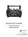
vpwl vin;
vin (n1, 0) { 2, 3;
4, -4;
6s, -4V;
8.0s, 1; }
The waveform of this voltage generator is given in Fig. 7.1.
Figure 7.1.
Waveform of piecewise-linear voltage generator, given by 4 time/voltage pairs.
106
Alecsis 2.3 - User’s manual
The waveform is given by time/voltage pairs. The pairs have to be enclosed in parentheses, regardless of the
number of points.
If the time instant of the first pair is greater than 0, the voltage value assumes the constant value between t=0
and the first pair, as in the example above. If the last time/value pair is before the tstop, the voltage keeps the
constant value until tstop. Therefore, if there is only one pair, such voltage generator behaves as ideal voltage
source of constant value. Similar rules apply for the current generator of type cpwl.
As any other voltage generator, vin in the example above generates link of type current. The current
carries the same name, vin.
The number of parameters of such generator is not fixed. However, it need not to be a built-in element.
AleC++ allows realization of a module where the action block has variable number of parameters (see
Chapter 5 for details):
module new_vpwl(node i,j) action(double time0, double value0, ...);
You need to use alternative syntax of determining of actual parameters (similar to function calls) and to
define some terminator (e.g., time moment -1), which will mark the end of the list. The call of such a component
would be:
#define EOL -1.0
new_vpwl vin;
vin(n1, 0) action(0ns, 1v, 10ns, 2v, 100ns, 2v, 110ns, 2.5v, EOL);
Keep in mind that compiler cannot check the type of parameters in the place of symbol '...'. That is, all
parameters, except the first two, have to meet expected types (double in this case). See Chapter 5 for details on
implementation of such action blocks.
7.1.2.4.
Sinusoidal signal generators
Alecsis has built-in voltage and current source of sinusoidal signal vsin and csin. The parameters are
amp (amplitude in V or A), freq (frequency in Hz), phase (initial phase shift in rad), and dc_offset (DC
component in V or A):
vsin vs;
vs
(n2, 0) { amp=2V; freq=1kHz; phase=30rad; dc_offset=0.5V; }
As any other voltage generator, vs in the example above generates link of type current. The current
carries the same name, vs.
7.1.3. Controlled sources
Controlled sources are implemented as built-in elements, too. The controlling quantity at the input is either
current or voltage, and the output quantity can be also either current or voltage. Therefore, there are four
combinations:
vcvs - voltage-controlled voltage source (takes parameter gain)
ccvs - current-controlled voltage source (takes parameter mi)
7. Analogue simulation in Alecsis
107
vccs - voltage-controlled current source (takes parameter gm)
cccs - current-controlled current source (takes parameter beta)
vcvs
ccvs
vccs
cccs
vg1
vg2
cg3
cg4
vg1;
vg2;
cg3;
cg4;
(n1, 0,
(n5, 0,
(0, n2,
(0, n2,
n3, n4) gain = 2;
vg1) mi = 1.2;
n3, n4) gm = 1e-4;
vg2) beta = 50;
The first two actual links in all examples above are of type node. Voltage source vg1 has n1 as positive
terminal, and vg2 has n5 as positive terminal. Currents of both current sources cg3 and cg4 assume direction
from 0 to n2 as positive.
Current-controlled sources vg2 and cg4 have one more actual link of type current, which is the
controlling variable. Voltage-controlled sources have two actual links of type node for control. Both sources vg2
and cg3 are controlled by the difference of voltages at nodes n3 and n4.
The example shows that voltage sources of type vcvs and ccvs generate new currents. They are here used
for control of generators of type ccvs or cccs.
7.1.4. SPICE-compatible nonlinear components
Circuit simulator SPICE has become a standard for circuit simulation. The biggest quality of this simulator
are the models of nonlinear electronic components. For that reason, we have implemented the same models (as
built-in models) in Alecsis.
For these models, Alecsis accept unmodified SPICE model cards. The keyword spice is used for that. For
instance, if file mosfet.mod, located in the working directory, contains models of MOS transistor given in
SPICE syntax, it can be included in your description using:
spice {
# include "mosfet.mod"
}
7.1.4.1.
Diode
Declaration of semiconductor diode utilizes the key word diode. A diode has two nodes -- anode and
cathode, given in that order, and a model card of class d. The list of model card parameters, together with their
default values, is given in Appendix.
diode d1, d2;
d1 (n1, 0) model = _1n914;
d2 (n2, n1) model = by238;
108
Alecsis 2.3 - User’s manual
7.1.4.2.
MOS transistor
Declaration of metal-oxide-semiconductor field effect transistor (MOSFET) utilizes the key word mosfet.
MOS transistor has four terminal nodes -- drain, gate, source, and bulk, given in hat order, which is adopted from
SPICE. It also accepts a model card of class nmos/pmos (the same model parameters, but for n and p type of
transistor channel).
Alecsis supports 4 types of MOS transistor models. There are three SPICE2 models (model parameter
LEVEL is 1-3), and also a BSIM model (Berkeley short-channel IGFET model) for transistors with submicron
dimensions. According to HSPICE classification, BSIM model cards have the LEVEL parameter set to 13.
Regardless of the level, MOS transistors have geometric parameters for length (l), width of the channel (w),
area (ad, as) and circumference of drain and source (pd, ps). Channel length and width must be given, while
other parameter have default value of 0.
mosfet m1, m2;
m1(n1,n2,0,0) { model=nes2mos; l=2u; w=6u; ad=as=10p; pd=ps=40u; }
m2(n3,n4,n2,0) { model=pes2mos; l=w=3u; }//other parameters are 0
Note:
MOS transistor models LEVEL 1, 2, and 3 have parasitic capacitances implemented as nonlinear
capacitors, whose capacitances are calculated for given terminal voltages. This is so-called Meyer model, which
exhibit charge nonconservation. Only BSIM (LEVEL=13) model has correct parasitic capacitance model, where
charge conservation is guaranteed. In this model, terminal charges are calculated rather than capacitances, and
parasitic currents are derivatives of these charges. Terminal charges can (optionally) appear as independent
variables in the circuit system of equations (see section on options in Chapter 5).
Any SPICE manual will offer additional information on the names of parameters in cards, their typical
values, and the appropriate equations for different levels. We give the list of model parameters and their default
values in the Appendix.
7.1.4.3.
Bipolar junction transistors
For declaration of bipolar junction transistor, keyword bjt is used. There are four terminal nodes -collector, base, emitter, and substrate, given in that order. The last node, substrate, can be omitted. It accepts
standard SPICE model card of class npn/pnp. Beside the model card, there is an optional parameter, area (area
of the transistor).
bjt q1;
q1 (c, b, e) model = bc1107a;
The list of model card parameters, together with their default values, is given in Appendix.
7.1.4.4.
JFET
For declaration of junction field effect transistor (JFET), keyword jfet is used. It has three terminal nodes
-- drain, gate and source, given in that order. It accepts standard SPICE model card of njf/pjf type. Parameter
area (area of the transistor) is optional.
7. Analogue simulation in Alecsis
109
njf j1;
j1 (d, g, s) model = J2N2068;
The list of model card parameters, together with their default values, is given in Appendix.
7.1.5. Ideal switch
Switch is implemented in Alecsis as ideal component, whose resistance is zero when the switch is closed (on
state) and infinite when it is open (off state). In Alecsis, switch is a voltage-controlled component. Unlike other ideal
switches this does not pose any limits in circuit topology. Even loops and cutsets of switches are allowed, providing
that the switching is regular. It can be used in both linear and nonlinear circuits. Switch is itself modelled as
nonlinear.
Note:
SPICE switch model has finite Ron and Roff resistances. Therefore, our switch model is not
compatible with SPICE. You can easily define your own SPICE-like model of non-ideal switch, as a resistor whose
resistance value is changed inside action block (see Section on combined structural-functional modelling on
how to do that).
Switch is declared using keyword switch.
switch sw;
sw (n1, 0, n2, 0) { hyst=1; val_on = 3.5v; val_off = 1.5v; }
Switch has four terminal nodes. The first two are contact nodes, connected by the switch (n1 and 0 in the
example above). The last two are controlling nodes - voltage between two nodes is the controlling voltage Vc. In the
example above, switch is controlled by the voltage at node n2, as 0 represents the ground node.
The switch has four parameters - val_on, val_off, hyst and paststate. The first two are the
thresholds, which are compared to the controlling voltage Vc. In most of the applications, these two thresholds are
equal, val_on = val_off. If Vc>val_on, the switch is closed. If Vc<val_off, the switch is open.
If val_on = val_off, parameter hyst plays no role. In the example above, you can see that
val_on can be different than val_off. When Vc is between these thresholds, the behaviour of the switch is
determined by the parameter hyst. This parametercan take values 0 and 1. If hyst is 1, the switch has
hysteresis. The switch state if Vc is between val_on and val_off depends on the switch history. It is allowed
both
that
val_on
>
val_off,
and
val_on < val_off in that case. If hyst=1, and val_on > val_off, the controlling of the switch is the
following:
•
when Vc is growing, when it passes the threshold val_on, the switch is turned on (closed);
•
when Vc is decreased, when it passes the threshold val_off, the switch is turned off (closed).
If hyst=1, and val_on > val_off, the control is somewhat different:
♦
when Vc is growing, when it passes the threshold (whatever comes first, val_on or val_off) the switch
is turned on (closed);
♦
when Vc is decreased, when it passes the threshold (whatever comes first, val_off or val_on), the
switch is turned off (closed).
If parameter hyst is 0 (which is the default value), the switch has no hysteresis. In this case, val_on
must be equal or greater than val_off. Between val_on and val_off, the switch has continuous change of
resistance. It should be noted that this is a continuous change between 0 (for val_on) and ∝ (for
val_off).
110
Alecsis 2.3 - User’s manual
Note:
Parameter hyst is optional, its default value is 0 (no hystersis).
Swtich also has parameter paststate. This is also an optional parameter. This parameter is actually not
used to pass information to the model. It is intended to be used in another direction -- it returns information about
the switch state in the previous (last solved) iteration.
In Alecsis, the switch is implemented as internally controlled, i.e. it is controlled by some circuit voltage. As
that voltage can change from iteration to iteration, it is clear that the final state of the switch can be determined only
when convergence occurs. In some cases, we want to know that switch state in the new iteration, and the parameter
paststate can be used for that. For instance, if we model the diode D as the ideal switch, the model can be
described as:
⎧closed , if p > 0
D:⎨
,
⎩ open, if p < 0
⎧ i if D is closed
p=⎨
,
⎩v if D is open
(7.1)
where i is the current through the diode (switch), and v is voltage on the diode (switch). The diode can be controlled
by voltage or current, depending on the diode state. To model it correctly using ideal switch, we have to know the
previous state of the switch.
module switch_diode (node a; node k) {
vgen vcaux;
switch sd;
vcaux (aux,0);
sd (a,k,aux,0) { val_on=val_off=0.5; }
action () {
process per_iteration {
if ( !sd->paststate ) {
/* switch was on (closed) */
if((current) sd>0) vcaux->value=1;
else
vcaux->value=0;
} else {
/* switch was off (open) */
if((node)a<(node)k) vcaux->value = 0;
else
vcaux->value = 1;
}
}
}
}
This is an example of combined structural-functional modelling that will be explained later in more details.
The structural part of the model introduces the switch sd, and the ideal voltage source vcaux, which is used for
switch control. (For diode model, we need switch controlled by the current. Switch is, however, implemented as
voltage-controlled element, so we need some auxiliary voltage (node aux) that will reflect changes of current). In
the structural part, generator vcaux is left without voltage value. This value is given in the functional part
(action block), as an implementation of formula (7.1). Parameter paststate is used to return state of the
switch in the previous iteration.
Note: The current through the switch is introduced as a new quantity in the system of equations (as was the
case with ideal voltage generators). In the above example, current sd was used in the action block.
We have tried to diminish differences between built-in component models and user-defined models
(modules). We have explained in Chapter 5, that the action parameters can be used bidirectionaly. As you can
see from this example, this is also the case with parameters of built-in components. Indirection operator -> was
used to access both the action parameters and the built-in component parameters.
The switch model was implemented as built-in, as it has some influence to time-step control. In some classes
of circuits, it was very important to simulate the switch just before the switch transition, and just after the switch
7. Analogue simulation in Alecsis
111
transition. It is important to simulate it just before the transition to obtain exact capacitor charges and inductor
fluxes in the moment of transition, as these quantities are of importance for the circuit after the transition. After the
transition, the time-step is reset, since the circuit has new topology. As the switches in Alecsis are internally
controlled, the exact switching instant is not known in advance. An iterative process is implemented to find the
switching instant with desired accuracy. See section on options in Chapter 5, where options SC_vtol,
SL_itol and SDDT_tol are described.
Note:
We have already stated that ideal switch model can be used in any circuit topology, even when
there are loops of switches and ideal voltage generators exist, or cutsets of switches and ideal current generators.
The condition is that the switching is regular. If it is not the case, the solver cannot converge, which should be
information for the user that there is problem with switching consistency (e.g. the part of the circuit is floating).
However, you should be aware that options for difficult convergence, dump and dcon, can sometimes force
convergence even in such cases. Therefore, they should be used with care.
7.2. Structural modelling
Many models can be described as connections of some other models, e.g. resistors, controlled sources, etc. If
we have a module, that has only declarative and structural part, and no functional part (no action block), we
consider that as a structural modelling. Both built-in components and user-defined modules can appear as parts of
such model.
module real_voltage_source (node 1, 2) {
resistor r1;
vgen vg;
vg(1,3) 5;
r1(3,2) 1k;
}
Node 3 is implicitly declared in this example.
Purely structural model is actually describing subcircuit, defining circuit hierarchy in that way.
7.3. Combined structural-functional modelling
In fully functional modelling, the user can write model equations freely in the action block. However,
this lack of restrictions can cause errors in the modelling process. Combined structural-functional modelling should
be the preferred way of modelling, as it is more restrictive, and therefore not so error-prone.
In the combined approach, the user gives the structural description of the model (like in the structural
modelling) but omit some or all of the parameters. These parameters are calculated and assigned to the components
later, in the functional part (action block). Such modelling technique is often used in electronics. An example is
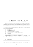
modelling of a nonlinear component, for instance diode, by linearizing it. Linearized diode model consists of a
resistor and ideal current source (Figure 7.1.). Parameters of these components Rdm and idsm are recalculated in every
iteration m using expressions (7.2) and (7.3)
112
Alecsis 2.3 - User’s manual
Figure 7.2.
Rdm =
Diode and its linearized model.
1
∂id
∂v d
m
ids
= idm −
(7.2)
vd =vdm
v dm
Rdm
(7.3)
Therefore, combined structural functional model of diode would consists of a resistor and ideal voltage
source connected in parallel, and an action block, where parameters of these components are calculated in every
iteration.
There is another reason to use combined approach instead of purely functional modelling whenever possible:
Alecsis can check circuit irregularities, such as loops of ideal voltage sources and inductors, or cutsets of ideal
current sources and capacitor, and inform the user about them. Such checking is possible when we use combined
modelling, since notion of these electronic components is still there. However, if we use equations, Alecsis cannot
recognize components in them.
In combined modelling, you need to reference elements inside a process to access them. The name of an
element in expressions is a pointer to the structure of element parameters. Some elements (resistor, capacitor, etc.)
have only one element in the structure -- value, while the others have more (named) parameters. For instance,
parameter value of resistor r1 is accessed as r1->value. All built-in element parameters are of double
type, and the parameters of user defined components (submodules) are given in their declaration.
The problem can arise with component that return current (or some other link), like voltage sources and
inductors are, since the names of element represent the current at the same time. Confusion is avoided as we can get
the current (or other link) using cast operation (for source v1 the current is (current)v1). Without cast, the
name represents the pointer to parameters.
7.3.1. Time-dependent linear models
We have already said that Alecsis has only ideal voltage and current source, and a pair of ideal signal
generators as built-in components. Using combined modelling approach with ideal source as a basis, any signal
generator can be easily described. To describe their behaviour, you often need only one process, and one line. For
modelling of linear generators process with per_moment synchronization is used. The process is
executed once in the given time instant.
#define twopi 6.282
module singen (node i, j) {
7. Analogue simulation in Alecsis
113
vgen gen;
gen (i, j);
action per_moment (double amp=1.0v, double freq=1kHz,
double phase=0.0rad, double offset = 0v) {
gen->value= offset + amp * sin( twopi*freq*now + phase );
}
}
root test () {
singen g1, g2;
g1 (node1,node2) { amp=0.2V; freq=50Hz; phase=0; offset=0.5V; }
g2 (node3,node4) action (0.2V, 50Hz, 0, 0.5V); // another way
...
}
This example shows the simplicity of modelling of sinusoidal generator with adjustable amplitude, offset,
frequency, and phase (all these parameters have default values, as well). As there is only one process , the
keyword process is not used, since the compiler takes the body of action with per_moment
synchronization
Name of voltage source gen is used as pointer to structure containing parameters. There is only one
parameter in the structure. That parameter can be reached using operator of indirection (->), i.e. as gen>value. In such case, when there is only one parameter in the structure, one can use indirection by dereferencing
(operator *), too:
*gen = offset + amp * sin ( twopi * freq * now + phase );
Built-in elements have their signals for synchronization. This is why linear and time-independent elements
behave as if they have processes sensitive to signal initial, in other words the contributions to the system of
equations are calculated only once. If we change values of parameters of such an element in the process
per_moment, like we do with the voltage source gen in the example above, we change their
synchronization to per_moment. In the same way, we can change synchronization of linear time-independent
and linear time-dependent models to per_iteration, if we change values of their parameters in a process
per_iteration. Nonlinear elements (transistors, diodes, etc.) cannot change their synchronization , as they
already have the most frequent refreshing, per_iteration.
Note: You may have noticed operator now inside the function sin. It simply returns the current time
moment of the simulation, which amounts to 0 for structural, post_structural and initial
processes. You can call it from any C/C++ -like function, but if the function has not been called during the
simulation the value of the operator will be 0.
Note:
In the structural description, parameter values need not to be omitted. If parameter value is
assigned in functional description (action block), the value given in structural part is overwritten. The value
assigned in the structural part is valid before the first execution of appropriate functional description. If no value is
assigned, 0 is assumed until the first execution of functional description. It is useful to assign nonzero values in the
case when zero values lead to singular matrix, which would abort the program in the phase of matrix renumeration
(only processes with synchronization structural are executed before the renumeration).
7.3.2. Nonlinear models
All built-in nonlinear components are modelled in Alecsis using Newton-Raphson method of linearization.
We can use Newton-Raphson method to linearize nonlinear models before composing equations, rather than to
114
Alecsis 2.3 - User’s manual
linearize nonlinear equations. You need to create a linearized scheme representing nonlinear component, where
linear components in that scheme change values of parameters in every iteration. Iterations are repeated until
convergence is reached.
We have already described such method in this section, using diode model as an example (Fig. 7.2.). The
parameter values of linear components are obtained by differentiating nonlinear functions. Therefore, model of any
nonlinear component can be described by declaring and connecting components of the linearized circuit, followed
by calculations of differentials in every iteration. Differentiation has to be performed with respect to all controlling
quantities, i.e. quantities that appear in the original nonlinear expressions. Often, all terminal quantities of that
nonlinear component are the controlling quantities.
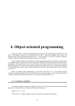
We shall give here example of a MOS transistor. This is the simplest version of MOS transistor model,
SPICE level 1 (Shichman-Hodges) model, without parasitic capacitances. Model is given as dependence of drain
current ID on all terminal voltages. This nonlinear model has to be linearized with respect to all controlling
quantities. If we consider source S as referent voltage, there are three controlling voltages - VGS, VDS, VBS. Linearized
model is given as a parallel connection of three voltage-controlled current sources, and one independent current
source (Figure 7.3.). Their parameters are recalculated in every iteration m using expressions (7.4.-7.7.).
Figure 7.3.
g mm =
m
g ds
=
∂I D
∂VGS
∂I D
∂V DS
m
g mbs
=
MOS transistor and its linearized model.
(7.4)
m
m
m
VGS =VGS
,VDS =VDS
,VBS =VBS
(7.5)
m
m
m
VGS =VGS
,VDS =VDS
,VBS =VBS
∂I D
∂V BS
(7.6)
m
m
m
VGS =VGS
,VDS =VDS
,VBS =VBS
m
m m
m
m
I Sm = I Dm − g mmVGS
− g ds
VDS − g mbs
VBS
(7.7)
MOS model has a number of technological parameters. Those parameters should be grouped in model card.
A class containing these parameters is defined firstly. Model code is then described using functions that are methods
of model class. These functions have access to parameters. Processes become shorter when bulk of the calculations
is performed in methods.
The following example gives a functional description of MOS transistor:
#define Ntype 1.0
#define Ptype -1.0
7. Analogue simulation in Alecsis
115
class simple_mos {
// new class of model cards
double type, gamma, phi;
double uo, vto, lambda;
public:
simple_mos ();
>simple_mos ();
~simple_mos ();
friend module smos;
};
simple_mos::simple_mos () { // constructor sets the initial values
type = 0.0 ;
gamma = 0.7 ;
phi
= 0.5 ;
uo
= 0.06;
vto
= 1.0 ;
lambda = 0.0 ;
}
#define
max(x,y) ((x)>(y)?(x):(y))
module simple_mos::smos (drain, gate, source, bulk) {
vccs e_gm, e_gmbs, e_gds;
cgen e_iaux;
/* linear voltage-controlled sources */
e_gm
(drain, source, gate, source) gm=0.0;
e_gds (drain, source, drain, source) gm=0.0;
e_gmbs (drain, source, bulk, source) gm=0.0;
/* ideal current source */
e_iaux (drain, source);
action per_iteration ( double w, double l ) {
double vto_mod, vd, vg, vs, vb, vds, vbs, vgs;
double sarg,von,vgst,arg,beta,betap;
double gm, gds, gmbs, ids;
vd = drain;
vg = gate;
vds = type * (vd - vs);
vgs = type * (vg - vs);
vs = source;
vb = bulk;
vbs = type * (vb - vs);
vto_mod = type * vto;
beta =w/l*uo;
if (vbs<=0.0) sarg=sqrt(phi-vbs);
else {
sarg=sqrt(phi);
sarg -= vbs/(sarg+sarg);
sarg=max(0.0,sarg);
}
von=vto_mod+gamma*(sarg -sqrt(phi));
vgst=vgs-von;
if (sarg<=0.0) arg=0.0;
else arg=gamma/(sarg+sarg);
if (vgst<=0.0) {
/*
cutoff region
*/
ids = gm = gds = gmbs = 0.0;
}
else {
betap=beta*(1.0+lambda*vds);
if (vgst<=vds) {
/*
saturation region
*/
double vgst2;
116
Alecsis 2.3 - User’s manual
vgst2= 0.5*vgst*vgst;
gm
= betap*vgst;
gmbs = gm*arg;
ids
gds
= betap*vgst2;
= lambda*vgst2;
}
else {
/*
linear region
*/
double betap_vds,vdsh, arga;
betap_vds=betap*vds;
vdsh = 0.5*vds;
arga = vds *(vgst-vdsh);
ids = (gm=betap_vds)*(vgst-vdsh);
gds = betap*(vgst-vds)+lambda*beta*arga;
gmbs = gm*arg;
}
}
/*
update element values
*/
e_gm->gm = gm;
e_gds->gm = gds;
e_gmbs->gm = gmbs;
*e_iaux = type *(ids - gm*vgs - gds*vds - vbs*gmbs);
}
}
model simple_mos :: simnmos { type=Ntype;
vto = 0.82; gamma=0.59; phi=0.686; uo=0.051; lambda=0.051;
}
model simple_mos :: simpmos { type=Ptype;
vto = -0.84; gamma=0.933; phi=0.733; uo=0.021; lambda=0.05; }
root module test () {
smos m1, m2;
m1 (n_out, n_in, 0, 0) { W=5u; l=3u; model=simnmos; }
m2 (n_out, n_in, n_Vdd, n_Vdd) { W=5u; l=3u; model=simpmos; }
...
}
Note:
In the structural description, parameter values need not to be omitted. If parameter value is
assigned in functional description (action block), the value given in structural part is overwritten. This is the
case with values for gm given in the structural part to sources e_gm, e_gds and e_gmbs in the example above.
The value assigned in the structural part is valid before the first execution of appropriate functional description. If
no value is assigned, 0 is assumed until the first execution of functional description. It is useful to assign nonzero
values in the case when zero values lead to singular matrix, which would abort the program in the phase of matrix
renumeration (only processes with synchronization structural are executed before the renumeration).
7.3.3. General nonlinear sources (automated linearization)
The linearization performed on MOS transistor model in the previous example means that we use NewtonRaphson method. The drawback is that the user is responsible to define both the structure of the linearized circuit,
and to define partial derivatives with respect to all controlling variables.
To make description of nonlinear models less error-prone and more user-friendly, we have developed special
nonlinear controlled generators, where the process of linearization is performed automatically. These are:
7. Analogue simulation in Alecsis
♦
nlcgen
- general nonlinear current generator;
♦
nlvgen
- general nonlinear current generator;
♦
nlgen
- general nonlinear equation.
117
In these nonlinear controlled generators, the user supplies only the nonlinear dependence, and Alecsis
estimates partial derivatives, replacing them with appropriate finite differences. Alecsis is able to calculate these
finite differences automatically. That means that the secant method is used for solving nonlinear problems in that
case. Newton-Raphson method has quadratic convergence (error in the next iteration is equal to the square root of
the error in the previous iteration). Secant method has lower order of convergence -- 1.62, instead of 2. Therefore,
order of convergence is decreased.
Note:
If we have a nonlinear circuit, usually only some of the models are described using nonlinear
generators nlcgen, nlvgen, and nlgen. Other, for instance, built-in models use Newton-Raphson
linearization. Therefore, the actual decrease of the convergence rate is low, and depends on the problem.
Since Alecsis estimates partial derivatives numerically, the nonlinear dependence can be even nondifferentiable (it is, however, understandable that non-differentiable functions with very strong nonlinearities
would lead to convergence problems).
In all three types of nonlinear generators, there can be any number of controlling links (the only
constraint is that there should be at lest one controlling link). Besides, type of controlling links is not
constrained, too -- they can be of any analogue type (node, current, charge, and flow).
We shall now describe syntax of each type of nonlinear generators in more details.
7.3.3.1.
Nonlinear current generator -- nlcgen
Nonlinear current generator has two nodes for connection, denoting where the generator current is flowing,
and at least one controlling link (of any analogue type). The connection nodes are given first. The order of
connection nodes is important, since it gives direction for current, as in any other current generator. The order of
controlling links is arbitrary. If the connection nodes are also controlling (i.e. if the value of the current depends on
connection nodes), they has to be stated again as controlling nodes).
In the structural part of the model, nonlinear generator is given without any parameters - only its connection
is defined. The nonlinear dependance of the current is given in the functional description, i.e. in the action
block. A process synchronized per_iteration has to be used, as dependence is nonlinear.
The example of MOS transistor model using nlcgen.
module simple_mos::smos (drain, gate, source, bulk) {
nlcgen mos_current;
mos_current (drain, source, drain, gate, source, bulk);
/* current flows between drain and source, and is controlled
by node voltages drain, gate, source and bulk */
action per_iteration ( double w, double l ) {
...
... // calculates ids without derivatives - skipped here
nlcgen mos_current = type * ids;
}
}
118
Alecsis 2.3 - User’s manual
The current flows between nodes drain and source, and the voltages of all for connections control it.
As drain and source are controlling voltages, too, they are repeated in the set of controlling links. In the
structural part of the module, no parameter is assigned to the nonlinear generator. The current value is calculated
in the process synhronized per_iteration. In the same process, value is assigned to the generator using its
name. In our example this was:
nlcgen mos_current = type*ids;
In simpler cases, the whole calculation can be performed on this assignment, so that the process contains
only one line of the code.
Note: Assignment operand (=) must not be understood literally here. The current is not actually assigned a
value, partial derivatives are calculated and the contributions are added to the system of equations (so-called model
stamp).
There can be any number of nonlinear generators declared inside one module. However, in the action
block of the module, each nonlinear generator value is calculated inside separate process. In every iteration,
Alecsis executes that process code more than once, to estimate partial derivatives. Therefore, each nonlinear
generator needs its own process, and all calculations regarding this generator should be in that process.
Therefore, there has to be one, and only one process per nonlinear generator:
module two_generators (node n1, n2, n3; current c3; flow f4) {
nlcgen gen1, gen2;
gen1(n1, n2, c3, f4);
gen2(n1, n3, n2, c3, n4);
action () {
process per_iteration {
nlcgen gen1 = c3*f4;
}
process per_iteration {
nlcgen gen2 = 5.*n2 - 6.*c3*n4;
}
}
}
Keyword nlcgen and component name (gen1 or gen2) give information to Alecsis which process to
connect with particular nonlinear generator.
Some special cases of controlled sources behave as basic components. So, nlcgen controlled by its own
voltage behaves as a resistor:
module new_resistor (node n1, n2) {
nlcgen r1;
r1(n1, n2, n1, n2);
action (double value) {
process initial {
if (value == 0.) warning ("zero resistance", 0);:
}
process per_iteration {
nlcgen r1 = (n1-n2)/value;
}
}
}
7. Analogue simulation in Alecsis
119
You can also model easily current-controlled and voltage-controlled current source (cccs and vccs).
However, in all these examples, synchronization per_iteration is used for otherwise linear and constant
models, which makes such description inefficient.
Nonlinear generator frees the user from determining structure of the linearized model and from calculating
partial derivatives. Nevertheless, you can use nonlinear generators in a different way, with user-defined partial
derivatives. In this way, only the structure of the linearized model is determined automatically. The user has to
define partial derivatives, and the Newton-Rahpson method is used, with quadratic convergence. The following
example demonstrates modelling of a diode:
module new_diode (node an, ch) {
nlcgen Id;
Id (an, ch, an, ch);
/* current flows from an to ch, controlled by
node voltages an and ch */
action (double is=1e-14) {
process per_iteration {
double vt = 25.8mV;
double gd, id;
id = is*(exp((ah-ch)/vt) - 1);
gd = (id + is)/vt;
nlcgen Id = id { @an = gd; @ch = -gd; }
}
}
}
With this description, simulator knows that source Id has the value id, and partial derivatives with respect
to controlling links an and ch in every iteration. Operator @ is used with controlling link name to denote partial
derivatives of a nonlinear function with respect to a particular link. If you omit the block containing partial
derivatives, the secant method is used:
...
nlcgen Id = id;
When partial derivatives are explicitely stated, the restriction about the number of nonlinear defined sources
in a single process does not apply (the process is now executed only once in every iteration).
If at least one partial derivative is explicitly given, Alecsis does not
estimate numerically other partial derivatives (which are not given).
Therefore, they are undefined, which can cause simulation errors.
Therefore, nonlinear generators have to be used with all partial
derivatives (partial derivatives with respect to all controlling links)
omitted, or with all derivatives explicitly calculated.
Alecsis does not give any warning about possible errors when only some
of the partial derivatives are calculated. We will improve this in next
versions.
120
Alecsis 2.3 - User’s manual
7.3.3.2.
Nonlinear voltage generator -- nlvgen
Nonlinear voltage generator has two nodes for connection, and at least one controlling link (of any analogue
type). The order of connection nodes is important, since it gives orientation of the generator (positive node first).
All other rules and restrictions are the same as for nonlinear current generator (nlcgen).
root module an_example_for_nlvgen () {
nlvgen nonlinear_vgen;
vgen v1, v2;
resistor r;
v1(n1, 0) 2;
v2(n2, 0) 3;
nonlinear_vgen(a,0, n1, n2);
r(a,0) 1.k;
timing { a_step = 1.; tstop = 100.; }
// current through nlvgen is available under its name
plot { node a; current nonlinear_vgen; }
action {
process per_iteration {
nlvgen nonlinear_vgen = n2*n3;
}
}
}
This is a very simple example with nlvgen, which here multiplies two voltages (2 and 3 volts), giving
result of 6. As for any other voltage source, current through nlvgen is introduced as new analogue link in
the system of equations. Here, current nonlinear_vgen is plotted out, and its value is 6mA.
Nonlinear voltage generator can be also used with user-defined partial derivatives, using the same syntax as
for nlcgen.
7.3.3.3.
Nonlinear equation -- nlgen
Nonlinear equation (nlgen) has somewhat different usage than nlcgen and nlvgen, although it
follows the same syntax rules. It has no connection nodes, but has an arbitrary number of control links. It creates a
new analogue link of type flow, which carries the same name as the generator. All contributions to the system
matrix are in the same row, which corresponds to this new flow. For that reason, we can say that nlgen creates
new (linearized) equation in the system matrix.
# include <math.h>
// includes declaration for sqrt function
module nlgen_test (flow f1, f2) {
nlgen gen;
gen(f1, f2); // f1 and f2 are controlling flows
action per_iteration {
nlgen gen = sqrt(n1*n2);
}
}
// new equation
7. Analogue simulation in Alecsis
121
In this example, equation gen=(n1*n2)1/2 is created, and is added (in linearized form) to the system of
equations. Obviously, unlike nlvgen and nlcgen, generator nlgen does not correspond to any electrical
element. As it creates new quantity of type flow (in our case, flow gen), it is to be used for modelling of
nonelectrical problems.
Other rules and restrictions are the same as for nlcgen and nlvgen. Generator nlgen can be used with
defined partial derivatives, too.
Note:
As automatic linerization is very convenient for users, we would create other forms of automated
linearization in the following versions of Alecsis. This wouls be automated linearization in purely functional
modelling (command eqn).
7.3.4. Virtual synchronization of processes
It is already explained that combined structural-functional modelling is based on connecting some built-in, or
previously modelled components, and than changing their parameters in the functional part of the description
(action block).
All built-in components have their internal synchronization -- resistors are filled into the system matrix as
processes initial, capacitors as processes synchronized per_moment, etc. When such built-in components
are used in the structural part of model, their synchronization can be changed in the functional part. For instance, if
linear and time-independent built-in component is used as part of the linearized model, their parameters are updated
in every iteration when they are referenced in process per_iteration. Naturally, re-synchronization is
possible only from less frequent to more frequent synchronization level (e.g. if nonlienar components are referenced
in process initial, they would be still updated in every iteration).
On the other hand, user defined models have processes with fixed syncronization. For instance, we can have
model described using fully functional modelling (explained later in this Chapter) with process initial:
module constant_component (node n1, node n2) {
...
action (double value) {
process initial {
...
}
}
}
When describing some other model using combined approach, we can use a component of type
contant_component as submodel. However, the problem can arise, since synhronization is here fixed, and
no re-synchronization is possible. We want user-defined models to behave in the same manner as built-in
components, and to be used equally. To enable that, we can add word virtual before the word process:
module constant_component (node n1, node n2) {
...
action (double value) {
virtual process initial {
...
}
}
}
Such process will behave as ordinary process initial, if you set the component parameter
value when connecting the component, and do not change it afterwards. However, if the parameter value is
122
Alecsis 2.3 - User’s manual
changed in a higher-order process (per_moment, per_iteration), the virtual process will be
re-synchronized to that more frequent synchronization level.
If parent component is digital (processes are sensitive to changes on signals), such child virtual
process initial would be re-synchronized to per_moment. The parameter value would be then
updated when the parent process activates (when there is change on signal the parent process is sensitive
to). However, the child process would be executed in every time-instant (per_moment synchronization), in
order to fill the analogue system matrix.
Processes sensitive to signals cannot have virtual synchronization.
7.4.
Functional modelling -- eqn statement
In fully functional modelling, user can freely write the equations that contribute to the system of equations.
Therefore, there are no restrictions in what is to be described as a model.
Note:
Lack of restrictions makes functional approach very powerful, but also error-prone. Alecsis, for
instance, check if there are any loops of ideal voltage generators and inductors, or cutsets of ideal current sources
and capacitors, etc. However, in fully functional modelling, there is no information about the model structure, so
such checking is not possible. Therefore, one can make an error in eqn statement and create singular system of
equations.
Equations are written using command eqn. They are written in the processes of the action block.
Therefore, structural part of the model can be completely omitted. There are three basic forms of this command:
simple eqn statement;
through eqn statement;
across eqn statement.
Simple eqn statement defines a single equation. All contributions to the matrix are in the same row.
Through eqn statement defines the current flowing through the branch between two specified nodes. It has
contributions in two rows, corresponding to these two nodes, and can be replaced by two simple eqn statements.
Across eqn statement defines the voltage across the branch, between two specified nodes. It has
contributions in three rows, corresponding to these two nodes and to the current flowing between them. Therefore,
an across eqn statement can be replaced by three simple eqn statements.
Electrical current is therefore a through quantity, while the voltage is an across quantity. Such approach can
be used in other physical problems, since we can define through and across quantities in them. Few examples are
given in Table 7.1.
7. Analogue simulation in Alecsis
123
Table 7.1. Across and through quantities in different physical domains.
generalized
quantities
electrical
mechanical translational
mechanical - rotational
hydraulic
etc.
across quantity
voltage V
velocity v
angular velocity ω
pressure p
...
through quantity
current I
force F
torque τ
flow Q
...
power
P=V I
P=v F
P=ω τ
P=p Q
...
For across quantity, an equation equivalent to Kirchhoff Voltage Law is satisfied, while through quentities
must satisfy an equivalent of Kirchhoff Current Law. If the designer of electrical or nonelectrical models uses such
paradigm of modelling, consistent system of equations will be built by Alecsis. Through and across εθν statements
are more restrictive than simple eqn statement, but they lead to better models.
Note: Using eqn statements, linear differential equations can be described. Nonlinear equations cannot be
described directly. Linearization of the model, according to Newton-Raphson method, has to be performed by the
user. Such linearization and eqn statement have to be in process synchronized per_iteration. In the
following versions of Alecsis, we plan to introduce nonlinear eqn statement, that uses the mechanisms developed
for nonlinear generators (nlgen).
7.4.1. Simple eqn statement
An example of simple eqn statement is the following:
eqn i: g*{i}-(2*v-8.)*{j}-4*{k}+5.-g*j=67.;
In this equation, contributions to the system matrix are defined. They are all in the row specified directly
after keyword eqn, i.e. in the i-th row. The column where the contribution appears is given by the index in
parentheses '{', '}', which multiplies the contribution. Expression g*{i} means that there is contribution g in the
i-th
column.
So
we
have
contribution
(-2*v+8.) in the column j, and -4 in the column k. All indices representing row and column, must be declared
as analogue links (node, current, charge, or flow), so that a row and a column in a matrix corresponds to
each of them.
Contributions that do not multiply any index in parentheses, are contributions to the right-hand side of the
system of equations. So, in our example we have contribution to the right hand side of the row i, which is (675+g*j). Note that j is here given without parentheses, which means that this is not a position in the matrix, but
the number of type double, which represent the current value (last solution) of the analogue link j.
Note: The contributions to the columns must be before the symbol '=', while the contributions to the righthand side vector can appear both before and after the symbol '='.
If the above equation is the only one that contributes to the row i, then the equation appear as such in the
system of equations. Nevertheless, other eqn statement in the same or some other module, or any other built-in or
user-defined model, can contribute to the same row. All these contributions are added to the row i, following the
concept of "stamps" common in electronic simulation.
We can form a stamp for any model using eqn statement. Here is an example of resistor:
module new_resistor (node i, j) {
124
Alecsis 2.3 - User’s manual
action (double value=0.0) {
process structural {
if (!value) warning("zero valued resistor", 1);
}
virtual process initial {
double g = 1/value;
eqn i: g*{i}-g*{j}=0;
eqn j: -g*{i}+g*{j}=0;
}
}
}
The first eqn statement contributes to the row i, and defines the current flowing through the resistor branch
from node i to node j. The same applies to the second eqn statement, but this defines current flowing from j to
i.
Expression g*{i}-g*{j} is the current that is flowing out of node i. If eqn i would be the only
one that contributes to matrix row i, we would have that this current is 0, which is senseless. But other components
connected to the node i contribute to that eqn, and the complete equation is stating that the sum of all currents
flowing out of node i is zero (Kirchhoff Current Law). For such case, when we are modelling currents or
voltages, it is much more readable, and less error-prone, to use through eqn statement or across eqn
statement, described in the following sections. Simple eqn statement should be used only when we are not
using Kirchhoff Laws or its equivalents described in Table 7.1., and that should be avoided if possible.
Equation
eqn i: g*{i}-g{j}=0;
can be also written as:
eqn i: g*{i,j}=0;
which makes equations shorter.
If i and j are links of type node, this can be also written as:
eqn i: g*{i,j}.v=0;
Extension '.v' denotes voltage. In this case, Alec++ would check the type of i and j, and would exit and give an
error message if they are not of type node. It can be also written as:
eqn i: g*{i}.v-g{j}.v=0;
If i and j are declared as links of type flow (rather than node), you can use extension .a. So, the
appropriate equation would be:
eqn i: g*{i,j}.a=0;
or:
eqn i: g*{i}.a-g{j}.a=0;
Extension '.a' denotes nonelectrical variable of across type. Alecsis checks if i and j are declared as links of type
flow.
7. Analogue simulation in Alecsis
125
Note: Alecsis differs between electrical across quantity -- voltage (node) and electrical through quantity -current; but with nonelectrical quantities, there is no such differentiation (in this version of Alecsis). All of
them are of type flow, which can be used both as an across and as a through quantity.
As you can conclude from examples above, extensions '.v' and '.a' are optional, but are recommended, as
they reinforce type checking. If extensions are not used, Alecsis checks only if both links in the pair {m,n} are
links of the same type.
Analogue links in eqn statement -- for instance, nodes i and j in statement:
eqn i: g*{i,j}.v=0;
Note:
must be scalars, as they are representing rows and columns in the system of equations. This applies for through and
across eqn statement, too.
Analogue links in eqn statement can be scalars that are member of
composite signals. Therefore, it is legal to define:
eqn w[2]: 5*w[2]-6*w[5]=32;
where w[2] and w[5] are scalar analogue links, members of link array
w[]. However, it is not legal to write:
eqn w[m]: 5*w[m]-6*w[n]=32;
since link array indices must be constant.
This problem can be avoided with one additional hierarchical level in
description. For instance, if you want to define:
process structural {
for (m=1; m<=k; m++)
for(n=1; n<=k; n++)
eqn w[m]: 5*w[m]-6*w[n]=32;
}
you have to define an additional module for equation:
module Equation (node w1, w2) {
action initial () {
eqn w[m]: 5*w[m]-6*w[n]=32;
}
}
and clone it in a loop, using clone command explained later in this
Chapter:
module Equation Eqn;
...
process structural {
for (m=1; m<=k; m++)
for(n=1; n<=k; n++)
clone Eqn(w[m],w[n]);
}
This applies on through and across eqn statement, too.
7.4.2. Numerical integration in eqn statement (ddt, d2dt2, idt)
Up to now, we have explained how to describe linear algebraic equations, that directly contribute to the
system of equations. However, many physical problems need differential equations to be modelled. Simple eqn,
126
Alecsis 2.3 - User’s manual
across eqn, and through eqn statements can be all modelled as differential equations. For example, capacitor
modelled using equation:
i=C
dv
dt
(7.8)
where i is the current through the capacitor, and v is the voltage accross its nodes, can be described as:
module new_capacitor (node i, j) {
action (double value) {
process per_moment {
eqn i: value * ddt{i} - value * ddt{j} = 0;
eqn j: -value * ddt{i} + value * ddt{j} = 0;
}
}
}
Equation (7.1) is a typical through equation, so it is better to use through eqn statement. This will be
explained in the next section.
Operator ddt stands for time derivative. It performs numerical integration (discretization). The numerical
integration method is chosen in the options block, which is explained in Chapter 5. The way of filling the matrix
depends on the method, but this is hidden from the user when operator ddt is used.
When operator ddt is used, contributions to the matrix is not constant - it depends on the time step, and on
the system history (solutions in the previous time instants). For that reason, in the above example, eqn command is
used in the process synchronized per_moment.
Shorter written is allowed here, too:
eqn i:
value * ddt{i,j} = 0;
as well as extension '.v' or '.a':
eqn i:
value * ddt{i,j}.v = 0;
The previous example of a capacitor can be modified, so that the current through the capacitor appears as
unknown in the system of equations. The stamp is 'expanded' for one row and one column, and these carry the name
of the current, which is here the same as the name of the component:
module current new_icap (node i, j) { // returns current on name
action (double value) {
process per_moment {
eqn i:
{new_icap} = 0;
eqn j:
-{new_icap} = 0;
eqn new_icap: value*ddt{i,j}.v -{new_icap} = 0;
}
}
}
The first equation is stating that the current flowing outside of node i is new_icap, the
second equation is stating that the current flowing outside of node j is -new_icap, and the
third one is describing current/voltage dependence given by eqn. (7.8).
Capacitor model given by eqn. (7.8) can be rewritten as:
7. Analogue simulation in Alecsis
v=
1
idt
C∫
127
(7.9)
That can be described using operator idt, which stands for integration with respect to time:
module newer_icap (node i, j) {
action (double value) {
process per_moment {
eqn i:
{newer_icap}=0;
eqn j:
-{newer_icap}=0;
eqn new_icap: {i,j}.v -1./value*idt{newer_icap}=0;
}
}
}
Operator idt is still not fully tested. Operator ddt is normally used for
all SPICE-like modelling and simulation problems.
For application in modelling of electronic components, operator ddt (time derivative) is enough, as there
are only first order differential equations. However, for modelling of mechanical systems, second time derivative is
often necessary. One could avoid usage of second-order time derivative by introducing additional equation.
Nevertheless, for the sake of model readability and to reduce size of the system of equations, we have introduced
second-order time derivative d2dt2:
process per_moment {
eqn x: m*d2dt2{x} + ro*ddt{x} + c*{x} - {F} = 0;
}
In this example of mechanical equilibrium m denotes the mass, ro is the friction resistance, and c is the spring
constant.
Operators ddt, d2dt2, and idt are connected to time-step control. Time-step control parameters are
given in Section 5.6.3.1. in Chapter 5.
Operators ddt, d2dt2, and idt cannot appear in arithmetic expressions outside of command eqn.
7.4.3. Through eqn statement
If we want to describe behaviour of a quantity that has through character (Table 7.1.), the simplest way to is
to use through eqn statement. For example, resistor model from section 7.4.1. can be described as:
module new_resistor (node i, j) {
action (double value=0.0) {
process structural {
if (!value) warning("zero valued resistor", 1);
}
virtual process initial {
double g = 1/value;
128
Alecsis 2.3 - User’s manual
eqn {i,j}.i = g*{i,j}.v;
}
}
}
Extension '.i' on the left-hand side of the equation denotes the current. The equation above means that the
current flowing between node i and node j equals g times the voltage between node i and node j.
Expression {i,j}.i reinforces type checking, as i and j must be links of type node (current can flow only
between nodes.
The through eqn statement above is fully equivalent to two simple eqn statements used for resistor model
in section 7.4.1. This equation can be also written as:
eqn {i,j}.i = g*{i}.v-{j}.v;
and to:
eqn {i,j}.i = g*{i,j};
which means that extensions on the right-hand side of the equation can be omitted. (They cannot be omitted on the
left-hand side of through equation.) The above equation can be also given with two through eqn statements.
eqn {i}.i = g*{i,j}.v;
eqn {j}.i = g*{j,i}.v;
where expression {i}.i on the left-hand side denotes the current flowing out of node i.
Many electrical models can be naturally described by through equation. For instance, statement:
eqn {i,j}.i = I;
describes current source of value I. It is equivalent to two simple eqn statement:
eqn i: 0 = I;
eqn j: 0 = -I;
It is clear that the through equation is much more readable, whenever the model represents the current through the
component as some function of controlling quantities.
An equivalent expression for nonelectrical quantities would be:
eqn {m,n}.t = g*{m,n}.a;
where extension '.t' denotes through quantity. The above equations means: through quantity flowing from flow
m to flow n equals g times the difference of across quantities m and n. Extension '.t' reinforces type checking,
so m and n have to be links of type flow (of across nature -- however, Alecsis does not differentiate between
across flows and through flows).
All variations of through equation, which are given above for currents and voltages, are valid for flows, too.
On the right-hand side, both nonelectrical and electrical variables can appear:
eqn {m,n}.t = g1*{m,n}.a + g2{i,j}.v;
This equations states that the through quantity flowing between flow m and flow n is the function of
across quantity between flow m and flow n, and of voltage between node i and node j.
7. Analogue simulation in Alecsis
129
Note:
Extension on the left-hand side of the through eqn statement ('.i' or '.t') cannot be omitted.
Only nodes or flows can appear on the left-hand side (it does not make sense to define the current flowing between
quantities of type current). On the right-hand side, extensions ('.v' and '.a') can be omitted, but are
recommended to reinforce type checking.
Note:
Extensions '.i' or '.t' can appear only on the left-hand side of through eqn statement. It does
not make sense to put expression {i,j}.i on the right-hand side of the equation, since current flowing between
nodes i and j is not available as the solution of the system of equations. If link k is of type current (for instance,
current through the voltage source named k), it can appear on the right-hand side of the equation, but without any
extension (extension '.i' would be confusing, since {k}.i denotes current flowing out of node k). For the
reasons explained in this Note, extensions '.i' and '.t' cannot be used in simple eqn statement at all).
Through eqn statement can describe differential equation, since operators ddt, d2dt2 and idt can be
used, too. Here is an example of capacitor model:
module new_capacitor (node i, j) {
action (double value) {
process per_moment {
eqn {i,j}.i = value * ddt{i,j}.v;
}
}
}
The model given above is fully equivalent to the first example from section 7.4.2. You can note that through
eqn statement given in this model clearly describe model given by eqn. (7.8).
7.4.4. Across eqn statement
As we are using nodal approach for solving the system of equations, we describe most of the models as
through equations (current as function of voltages). However some of the models cannot be described in this way.
For instance, all kinds of ideal voltage generators (independent and controlled) have to be described as voltage
dependence on other quantities. For that reason, we need modified nodal approach, where current through the
branch is added as an additional unknown in the system of equation, and branch voltage equation is added as
additional equation. This can be easily described using across eqn equation.
An ideal voltage source can be described in this way:
module current new_vgen (i, j) {
action (double value) {
virtual process initial {
eqn new_vgen, {i,j}.v = value;
}
}
}
Expression {i,j}.v = value gives the dependence of voltage between node i and node j (in
this case, this is a constant voltage). In through equation, current through the branch has also to be specified, since
this is the row in the system matrix where this equation is added. The name of the current is given after keyword
eqn, before the equation itself is given. In our example, the name of he current is new_vgen, and this is also the
name of the module, declared as the current (this returning the current on the module name will be
declared later in this Chapter). It is important that this variable, representing the current through the branch, is
declared as current before the functional description (action block).
Across eqn statement
130
Alecsis 2.3 - User’s manual
eqn new_vgen, {i,j}.v = value;
from the example above has the same contribution to the system of equations as three simple eqn statements:
eqn i:
eqn j:
eqn new_vgen: 1*{i} -1*{j}
1*{new_vgen} = 0;
-1*{new_vgen} = 0;
= value;
These two descriptions define the same model stamp.
Across equation:
eqn k, {i}.v = r*{k};
has the same effect as:
eqn k, {i,0}.v = r*{k};
since 0 is always representing ground node.
Across equation can be described for nonelectrical quantities (flows), too. An example is:
eqn k, {m,n}.a = r*k;
The quantity that represents difference of flow m and flow n equals r times quantity k. Links m and n
have to be of type flow, and of across nature, according to Table 7.1. (However, there is no difference between
across and through flows on declaration in this version of Alecsis). Link k has to be of type flow (of through
nature).
Note:
Extension on the left-hand side of the across eqn statement ('.v' or '.a') cannot be omitted.
Only nodes or flows can appear on the left-hand side. On the right-hand side, extensions ('.v' and '.a') can be
omitted, but are recommended to reinforce type checking.
Note:
This Note is the same as for through eqn statement: Extensions '.i' or '.t' cannot appear on the
right-hand side of across eqn statement. If link k is of type current (for instance, current through the voltage source
named k), it can appear on the right-hand side of the equation, but without any extension.
Across eqn statement can be differential, i.e. operators ddt, d2dt2 and idt can be used. We have
already defined model of a capacitor, with the current through the capacitor is added as unknown to the system of
equations, in section 7.4.2. (module newer_icap). This can be easily described using across eqn statement:
module newer_icap (node i, j) {
action (double value) {
process per_moment {
eqn newer_icap: {i,j}.v = 1./value*idt{newer_icap};
}
}
}
This across eqn statement clearly describes model given by eqn. (7.9).
For the capacitor model, we do not need current through the capacitor as new unknown in the system of
equation, so it is more natural to use through equation. However, to model inductance, we need that current, since
voltage is dependent on the current:
v=L
di
dt
(7.10)
7. Analogue simulation in Alecsis
131
The inductor model using across eqn statement is:
module current new_l (i,j) {
action (double value) {
process per_moment {
eqn new_l, {i,j}.v = value*ddt{new_l};
}
}
}
7.5.
Appointed simulation in a time-instant -- breakpoint
Alecsis works with variable time-step. Time step is changed to meet demands on numerical integration error.
For that reason, we cannot know in advance which time-instants would be chosen for simulation. However, in some
particular cases, we want to force Alecsis to perform simulation in some particular time-instants. Function
set_bpoint is used for that. It sets a breakpoint for a given time-instant (i.e. appoints simulation for that timeinstant).
For instance:
set_bpoint(now+Period);
appoints simulation for time instant that happens Period after current time (keyword now returns current
simulation time). Simulation proceeds with normal time-step control until it approaches the breakpoint, and then the
time step would be shortened to meet the breakpoint. That means, it will not be allowed to jump over the
breakpoint.
Function set_bpoint() can be used inside a process of action block.
An application example can be found in definition of module pulse (in file alec.hi in subdirectory
sys that is normally installed with Alecsis.). This is definition of voltage generator of trapezoidal waveform. If
time-step is large, corners of trapezoidal waveform can be missed. The simulation results are still correct, but the
waveforms that are plotted out are not always nice -- corners of trapezoidal waveform can be cut out. Function
set_bpoint is used here to force simulation in corners of trapezoidal waveform.
Note:
As simulation time is variable of type double in floating-point arithmetic, the appointed
breakpoints cannot be met exactly, due to some rounding errors.
7.6.
Returning the link using name of a module
We have already mentioned that some built-in elements have to be modelled using branch voltage equations.
For these elements, current through the branch has to appear as new unknown in the system of equations. That
current can be plotted out, or used as controlling current for other models, using the name of the built-in component.
This is the same as in SPICE.
Our concept was that user defined modules can be used equally as built-in component models. For that
reason, AleC++ allows that the module name return the current (similarly as functions return variables - but here, it
is not the value of the current that is returned, but the actual position in the matrix).
We have already given such examples in the previous section, for instance, ideal voltage source model:
132
Alecsis 2.3 - User’s manual
module current new_vgen (i,j) { // new_vgen is name of the current
action (double value) {
virtual process initial {
eqn new_vgen, {i,j}.v = value;
}
}
}
Here, current new_vgen is not declared separately, but when the module name is defined, as:
module current new_vgen
Current new_vgen can be used inside that module like any other current. However, when this module is
used to declare components of type module new_vgen, each component of that type returns the current on its
name:
module Y (node i,j,p,q) {
module new_vgen X;
// THIS DECLARES X AS CURRENT
ccvs Z;
// a current-controlled voltage source
X(i,j) action( 5);
Z(p,q,X) mi=1;
// current X is used for controlling
}
If we model the above voltage generator in the following way:
module newer_vgen (i,j) {
current k;
// separate declaration for current
action (double value) {
virtual process initial {
eqn k, {i,j}.v = value;
}
}
}
then no association between name of the module and name of the current is established. Voltage source
model is correct, but it does not return any current under its name, and cannot be used in our module Y.
This explains how to return current using the name of the module when the current is declared locally, inside
the given module. But what to do when this current is passed by another module? For instance, when current
returned by our module new_vgen has to be returned by our module Y, too. An association can be
established in such case:
module current Y (node i,j,p,q){ // Y is also an current,
module new_vgen Y;
// and it is returned by new_vgen
ccvs Z;
return Y(i,j) action( 5);
Z(p,q,Y) mi=1;
// keyword 'return' is necessary
}
In this example, module Y also returns current under its name. It is the current returned by module
new_vgen, and for that reason, component of type new_vgen also carries the name Y. When the component Y
is connected, keyword return has to be used before the name Y, to point out the association of the names.
(Without keyword return, Alecsis would consider this as name redeclaration, which is an error.)
This works in the same manner if we use built-in component (e.g. vgen), instead of user defined module
new_vgen.
The compiler will not allow association of more than one component with the name of a module.
7. Analogue simulation in Alecsis
133
If you consider this too complex, you can return the current using list of formal parameters:
module Y (node i,j,p,q; current X){ // formal param. X is current
module new_vgen X;
// and it is returned by new_vgen
ccvs Z;
X(i,j) action( 5);
Z(p,q,Y) mi=1;
}
Here, module Y does not return any current on its name, but it returns current using list of formal
parameters. As we have already explained, formal parameters of a module can be used for bi-directional
communication, unlike parameters of C-like function. They are passed by reference, not by value, as they are
representing position in the system of equations. Keyword return is here not used for association.
More than one component cannot associate with the same formal parameter, because that would be a name
redefinition in the same structural visibility area (every component has its own current -- for example, every
inductor has a current flowing through it.) It is not legal to associate with a formal parameter that is not a
scalar.
Note:
Links of type charge and flow can be returned using name of the module, too. All what is
here explained for links of type current, is also valid for charge and flow. However, this feature is
introduced for links of type current, to make Alecsis compatible with SPICE.
7.7.
Variable number of action parameters
The number of parameters in the header of the action block of the module can be variable. This is
described in the Chapter 5, as it is the same for digital and analogue modules.
7.8.
Modules with variable structure -- clone and allocate
Some complex models cannot be easily described using standard Alecsis syntax. Sometimes we want that
model card parameters or action parameters determine not only the behaviour, but also the structure of the
model. There are two cases when this can be necessary:
• When some subcomponents appear in the module structure conditionally, depending on the model card
parameters of action parameters. This can be, for instance, the case with resistances connected in series
on component terminals, that are usually optional; or with whole optional subcircuits, e.g. some
compensation subcircuits for opamps, etc.
• To define regular subcomponent arrays of variable size. Some electronic circuits exhibit clear regularity.
Therefore, one can describe an array of variable size, where the size is an user-defined parameter.
Command clone is used to describe such models. It defines cloning of the previously described or built-in
component. Cloning can be executed only in processes synchronized as structural, since execution of
command clone defines the structure of the circuit. As this command is used inside a process
(structural), it can be executed conditionally, or in a loop, depending on the user-defined parameters.
Note:
Models defined using command clone cannot be classified as either structural or combined
(structural-functional), since here execution of process structural determines structure of the model.
134
Alecsis 2.3 - User’s manual
The syntax of command clone follows all rules for component coupling:
clone_command:
clone body_of_command_clone
body_of_command_clone:
component ;
{ component_list }
component_list:
component ;
component_list component ;
When we use command clone to create arrays of variable size, it is clear that the number of links (e.g.
terminal nodes) cannot be known in advance, too. So we need a mechanism to handle arrays of links of variable
size. That dynamical allocation of link arrays is enabled using command allocate.
We can see application of both clone and allocate on the following example of ring oscillator:
module inverter(node vout, vin, vdd, vss) {
mosfet mup, mdown;
(vout, vin, vdd, vdd) { model=Mpmos; l=3u; w=8u; }
mup
mdown (vout, vin, vss, vss) { model=Mnmos; l=w=3u; }
}
module ring_oscillator (vout, vdd, vss) {
inverter inv;
node joint[auto];
// array of nodes (size not defined)
action (int size = 3) {
process structural {
allocate joint [size-1];
// dynamical allocation
int i;
if (size < 3 || size % 2 == 0)
warning("wrong number of inverters in ring", 1);
for (i=0; i<size; i++) {
if (i==0)
clone inv[0] (joint[0], vout, vdd, vss);
else if (i==size-1)
clone inv[i] (vout, joint[i-1], vdd, vss);
else
clone inv[i] (joint[i], joint[i-1], vdd, vss);
}
}
}
}
In this example, an MOS inverter is defined structurally, and that module inverter is used as
component to be cloned into an array. In module ring_oscillator we have component inv of type
inverter declared. We also have declaration of an array of nodes with the name joint. Command:
node joint[auto];
is declaration of one-dimensional array of nodes. Length of that array is not yet defined, it will be done using
command allocate.
7. Analogue simulation in Alecsis
135
We can note that module ring_ocillator has no structural part, i.e. declared component inv of
type inverter is not connected in the structural part.
Inside the functional part (action block) a process structural is defined. In that process, array
of nodes joint is allocated as:
allocate joint [size-1];
Array joint has length size-1, and zero-offset is used (from 0 to size-2). Parameter size is
passed as an action parameter (default value is 3).
Note: Array of links can be have more dimensions, can have lower limit defined, etc. (all rules for Alecsis
link array apply). Example:
allocate joint[1:size];
// array with offset 1;
When array of links has more than one dimension, only the first
dimension can be dynamically allocated. For example, you can declare:
node a[auto][j];
but you cannot declare:
node a[auto][auto];
We intend to improve it in following versions of Alecsis, but as it is a
complex intervention, it might wait for some time! (Array of links is very
different than array of variables in C/C++ - links are positions in the
system of equations.)
If you need to dynamically allocate array of links with more than one
dimension, you can either reorganize it as one-dimensional array (which
is always possible); or you can use array with static allocation, and
recompile the model when you change dimensions:
# define FIRST_DIM 150
# define SECOND_DIM 200
...
node a[FIRST_DIM][SECOND_DIM];
In our example of ring oscillator, parameter size is checked firstly (it cannot be an even number, if we
need an oscillator). After that, a for loop is defined, where size instances of component inv are cloned. A i-th
instance of component inv is connected between nodes joint[i] and joint[i-1] using command:
clone int[i] (joint[i], joint[i-1], vdd, vss);
Index [i] after component name int can be omitted. However, it is useful, as it enables us to approach
the particular component int[i] later -- in command plot, for instance.
This ring of inverters is a regular structure, but it has exceptions at the beginning, and at the end of the array
(connections to output node vout). This is handled using if/else commands.
From this example one can conclude that both the component to be cloned, and the array of links of variable
size, have to be declared in the declarative part of the module. The actual size of the link array, and cloning of
components, are in the action block, process structural.
136
Alecsis 2.3 - User’s manual
Note:
Action parameters of cloned components can be different. However, if the component that is
cloned has a model card, parameter model must be known in the compilation time (the model card name cannot be
passed as a variable).
In command:
clone int[i] (joint[i], joint[i-1], vdd, vss);
index [i] after component name int can be omitted. However, it is useful, as it enables us to approach the
particular component int[i] later -- in command plot, for instance. Index becomes a part of the component
name, and in command plot, it must be used inside quotation marks, without any blanks inside the quotations:
plot { node s1/s2/"comp[5]"/n1;
current "lserial[3]"; }
In the above commands, we use cloned component name to define absolute path (to local link node n1 in
the component "comp[5]"); or to get the values of current returned under module name
("lserial[3]").
Note: Commands clone and allocate apply to analogue, digital, and hybrid circuits in the same way, since
nowhere in the syntax does the command demand a particular link type or component type. It is especially useful in
digital simulation, for instance to describe registers of different lengths.