Download Post processing field spectra in MATLAB

The FSF Post Processing Toolbox User Guide
Post processing spectral data in MATLAB
I. Robinson and A. Mac Arthur
Field Spectroscopy Facility, Natural Environment Research Council
1. Introduction
The Field Spectroscopy Facility (FSF) Post Processing Toolbox is a MATLAB toolbox
containing functions for importing optical spectra from field-portable specroradiometers
and processing them. MATLAB is a computer environment and high-level programming
language which provides a flexible environment for processing spectra as well as a good
set of built-in data structures, functions and plotting tools. This toolbox is designed as an
add-on to MATLAB which will make it easier to import, examine and process data related
to field spectroscopy.
Spectra acquired in the field must be post processed to plot and examine spectra, remove
invalid data and apply equipment calibrations. MATLAB provides an ideal environment
for all these functions, as it provides a flexible environment and set of tools for importing,
plotting, analysing and processing data. This toolbox is designed to make the handling of
field spectra easier. It provides a number of functions to import the data file formats used
by various instrument manufacturers including:
• FieldSpec spectroradiometers manufactured by Analytical Spectral Devices (ASD)
• The GER 1500, GER 3700 and HR-1024 manufactured by Spectra Vista Corporation
(SVC)
• The OOI binary file format used by Ocean Optics SpectraSuite software
• The V–SWIR data file format used by the Field Spectroscopy Facility (FSF)
Once imported into MATLAB these data can readily be plotted or further processed. This
toolbox provides the following convenient processing functions to:
• Remove overlapped spectral data occuring at the join between different detectors
• Sort and pair target spectra with corresponding reference spectra using a logsheet
file
• Calculate a relative reflectance spectrum from paired target and reference spectra
• Calculate an absolute reflectance spectrum using calibration data for a reflectance
panel
• Remove erroneous spectral data caused by high absorption in the water bands
• Smooth spectra with a Savitzky–Golay filter
• Convolve spectra to the spectral response function (bands) of airborne and satellite
instruments
This document exlpains how to install the toolbox, how to handle and plot spectral data
using MATLAB structures and how to use the provided processing functions.
2 INSTALLING THE TOOLBOX
1.1. Contributor information and the User Group
This toolbox was developed by Iain Robinson and Alasdair Mac Arthur at the Field Spectroscopy Facility in Edinburgh. This work was supported by the Natural Environment
Research Council.
Some features of the function to read ASD binary files were based on code contributed by
Andreas Hueni from University of Zürich.
Spectral response functions for a number of satellite sensors was provided by Tim Malthus.
Guillaume Drolet, Julia McMorrow, Elizabeth Lowe and Reno Choi provided useful discussion about the convolution of spectral data with the spectral response functions of airborne
instruments.
Appendix B on using ViewSpec Pro was written by Peter Walker and Chris MacLellan.
The Field Spectroscopy Facility’s User Group provides a selection of useful utilities and
tools for the handling and processing of field spectra. We welcome all contributions whether
based around MATLAB or other platforms. Please contat us if you have any questions or
would like to contribute a resource.
1.2. Further information
An overview of field spectroscopy can be found in the recent review article by Milton [1].
A broad list of references is available from the Field Spectroscopy Facility’s web site. A
description of MATLAB is available from The MathWorks.
2. Installing the toolbox
This section describes how to install the toolbox on a system running MATLAB.
2.1. Check requirements
The toolbox requires MATLAB 7.8 (R2009a) or later, although some functions may work
with earlier versions. The Savitzky–Golay smooth function (sgsmooth) additionally requires the Signal Processing Toolbox.
For handling files from Analytical Spectral Devices (ASD) instruments ViewSpec Pro is
recommended to convert ASD’s binary format to the more easily-readible text format.
Calculation of absolute reflectance requires calibration data for the reference panel which
was used in the field. Calculation of radiometric spectra (radiance or irradiance) requires
calibration data for the specific instrument and configuration which was used.
Calibration data for the Field Spectroscopy Facility’s reference
panels and instruments is available.
Convolution of field spectra to the spectral response functions of airborne or satellite instruments requires the band data for the specific instrument. Data for a range of instruments
are available from the User Group.
2012-07-18
2
version 1.3.6
3 IMPORTING, EXAMINING AND PLOTTING
Figure 1: Add the directory containing the toolbox to the MATLAB search path. Additional documentation for the toolbox will appear in the help broswer.
2.2. Download and install
To install the toolbox first download and unzip the file, then add it to the MATLAB search
path:
1. Download FSFPostProcessing1.3.6.zip.
This zip file contains a folder called FSFPostProcessing1.3.6 which contains all the functions, documentation and examples in the toolbox.
2. Unzip the file in a folder which is accessible to MATLAB. (If MATLAB is running
on a server the toolbox files may need to be located on the server.)
3. In MATLAB: add the FSFPostProcessing1.3.6 folder to the search path. This can
be done using the Set Path tool which can be opened from the File menu, as shown
in Figure 1. Click Add folder, then locate the FSFPostProcessing1.3.6 folder. In
order to have MATLAB remember this new path, click Save before closing the Set
Path tool.
Once the toolbox is added to the search path the toolbox documentation will appear in the
help browser under ’FSF Post Processing Toolbox’ as shown in Figure 1. Further information about MATLAB’s file locations and the search path is available in the MATLAB
documentation.
3. Importing, examining and plotting
Once installed spectra acquired on field-portable spectroradiometers can easily be imported
from the data file into the workspace. This section describes how to import the files and
how to examine and plot the data in the MATLAB environment.
Reliable metadata is critical for field spectroscopy. All instrument data files contain important information in the file’s header. This includes details such as the date and time
the spectrum was recorded, the location it was recorded (for instruments with GPS) and
the instrument settings. The toolbox imports this information into a MATLAB structure,
along with the data itself.
A few example data files are provided with the toolbox to test these functions. These can
be found in the examples folder which is located within the folder where the toolbox was
installed (FSFPostProcessing1.3.0/examples).
2012-07-18
3
version 1.3.6
3 IMPORTING, EXAMINING AND PLOTTING
3.1. Importing spectral data files
Each instrument manufacturer uses a different data file format for field spectra. A separate
import function is provided for each and they are described in the following subsections.
3.1.1. Analytical Spectral Devices (ASD)
Files from ASD FieldSpec 3 and FieldSpec Pro spectroradiometers use a binary format
which must first be converted to text files using ViewSpec Pro1 . This tool is available from
ASD’s Support Central web site. At the time of writing the latest version was 5.6.10. The
procedure to convert binary files to (ASCII) text is described in Appendix B.
An ASD text file can be imported into MATLAB by typing:
s = importasd(f́ilename´
)
where filename is the name of the file to be imported. Multiple files can be imported at
once using wildcards. For example, if the current directory contains several ASD text files
with the .txt extension they can be imported by typing
s = importasd(´
*.txt´
)
The imported spectrum or spectra will be stored in a structure array in the workspace. If
output is not suppressed (with a terminal semi-colon) a struct array will be shown:
s =
96x1 struct array with fields:
name
datetime
header
wavelength
data
The type of data imported (into s.data) depends on the operating mode of the ASD
spectroradiometer. If the spectra were recorded in white reference mode the data values
will be reflectances (in the range 0–1) and further processing can continue. If the data
were recorded in raw mode 2 , the spectra must be sorted into reference and target spectra
before reflectance can be calculated. This process is described later.
3.1.2. Spectra Vista Corporation (SVC)
Files from SVC spectroradiometers (GER 1500, GER 3700 and HR-1024) are stored in the
signature text file format[2]. These files usually have a .sig extension. Each file contains
a header followed by a pair of spectra: one target spectrum and its corresponding reference
spectrum.
A SVC signature file can be imported by typing:
1
This toolbox has very limited support for ASD’s binary file format so conversion from binary to (ASCII)
text is recommended.
2
The importasd function automatically normalizes data recorded in raw mode to account different integration time settings on different detectors. The normalization method is described in detail in
Appendix A.
2012-07-18
4
version 1.3.6
3 IMPORTING, EXAMINING AND PLOTTING
Figure 2: Spectral data recorded in raw mode can be paired by creating a logsheet file.
[tar, ref] = importsvc(f́ilename´
)
where filename is the name of the file to be imported. Multiple files can be imported at
once using wildcards. For example, if the current directory contains several SVC text files
with the .sig extension they can be imported by typing:
[tar, ref] = importsvc(´
*.sig´
)
The imported spectrum or spectra will be stored in two separate structure arrays in the
workspace, one of target spectra (tar) and one of reference spectra (ref). If output is not
suppressed (with a terminal semi-colon) the structures will be shown:
tar =
1x7 struct array with fields:
name
datetime
header
pair
wavelength
data
ref =
1x7 struct array with fields:
name
datetime
header
wavelength
data
Note that the structure array of reference spectra (ref) may contain duplicates. This is
because signature files always contain the previously-recorded reference spectrum for each
target spectrum. Additionally the structure array of target spectra (tar) contains a field
called pair. The value of the pair field gives the name of its corresponding reference spectrum. This pairing information, which matches target spectra to their reference spectra,
is required for calculating reflectance.
2012-07-18
5
version 1.3.6
3 IMPORTING, EXAMINING AND PLOTTING
When importing spectra from SVC instrument models with multiple detectors, such as the
HR-1024, there may be overlapped data in the spectra. This occurs at the joins between
the different detectors. The removeoverlap function, described in Section 4.2, can remove
these data.
3.1.3. Field Spectroscopy Facility (FSF)
The FSF has developed a portable spectroradiometer called the Visible Short-wave Infrared
(V–SWIR) Spectroradiometer [3, 4]. The function importvswir imports data files in the
format [5] used by the instrument. V–SWIR data files usually have a .DTA extension.
A V–SWIR data file can be imported by typing:
[upwelling, downwelling] = importvswir(f́ilename´
)
where filename is the name of the file to be imported. Multiple files can be imported at
once using wildcards. For example, if the current directory contains several V–SWIR data
files with the .DTA extension they can be imported by typing:
[upwelling, downwelling] = importvswir(´
*.DTA´
)
The imported structure arrays contain upwelling and their corresponding downwelling spectra. If output is not suppressed (with a terminal semi-colon) then the structure arrays will
be displayed:
upweling =
1x100 struct array with fields:
name
datetime
header
pair
processing
wavelength
data
downwelling =
1x100 struct array with fields:
name
datetime
header
processing
wavelength
data
The V–SWIR instrument records a downwelling (reference) spectrum for every upwelling
(target) sectrum. There will therefore always be the same number of upwelling and downwelling spectra. The importvswir function does some basic processing of the spectra, such
as dark subtraction, automatically. The field processing contains the raw (unprocessed)
data.
For the V–SWIR instrument radiometric calibration data are available from the FSF. These should should be applied before calculating reflectance.
2012-07-18
6
version 1.3.6
3 IMPORTING, EXAMINING AND PLOTTING
3.2. Examining headers and data
Imported data are stored in MATLAB structure arrays. This ensures that header information (metadata) is kept together with the spectrum itself (wavelength and data). The
structure of the data and the ways to examine it are described in the following subsections.
3.2.1. Structure arrays
The spectra are stored in a MATLAB data type called a structure array. A single spectrum
is a single structure, whereas multiple spectra are grouped together, and numbered, in a
structure array. The structure is divided into fields which contain individual pieces of data.
A spectrum structure typically contains the following fields:
• name is the name of the spectrum (usually taken from the filename during importing)
• datetime is the date and time the spectrum was recorded3 .
• header is a structure containing all the header information (metadata) from the
original file.
• pair appears only in target spectra and gives the name of the corresponding reference
spectrum.
• wavelength is a column vector of wavelengths in nanometres.
• data is a column vector of the corresponding values. These will generally be uncalibrated digital numbers. For ASD spectrometers running in white reflectance mode
these values will be reflectances in the range 0–1.
It is straightforward to add additional information to existing structures if desired. For
example, to add a light reading (in lux) to an existing structure:
s.lux = 15000
A new field called lux would then be automatically added.
Further information on structure arrays is available in the MATLAB documentation.
3.2.2. Workspace browser
Once imported the spectra can be examined in the workspace browser. This can be opened
by selecting Workspace from the Desktop menu, or type the command workspace. The
spectra will be visible as structure arrays with the names given when imported. Doubleclick an array to browse its contents. If the strucure contains multiple spectra, they will
be listed as a row vector. Double-click again examine a specific spectrum.
More information on using the workspace browser is available in the MATLAB documentation.
3
The source of this data may be the spectrometer’s internal clock, or may be the clock of the computer
or PDA used to record the spectrum.
2012-07-18
7
version 1.3.6
3 IMPORTING, EXAMINING AND PLOTTING
Figure 3: Use the headers function to combine all headers into a single table.
3.2.3. Comma-separated lists
A specific field of a structure array can be accessed as a comma-separated list. For example,
if s is a structure array of spectra, typing:
s.name
produces a comma-separated list of the names of all the spectra:
ans =
gr061110_000_reference
ans =
gr061110_001_reference
...
Comma-separated lists can easily be assigned to variables. To store the above list in a
variable called allnames type:
allnames = {s.name}
The curly brackets ({}) in concatenate the list into a cell array.
Using comma-separated lists provides a way to rearrange imported data in any format
or structure that may be required. It is particularly useful when dealing with a large
number of spectra as described in the following subsections. Further information about
and examples of comma-separated lists are available in the MATLAB documentation.
3.2.4. Creating a table of header information
When a large number of spectra have been imported it may be convenient to summarize all
header information in a single table, as shown in Figure 3. The headers function provides
a convenient way to produce a cell array containg the values of all the header fields.
To create a cell array of header information H from a structure array s, type:
2012-07-18
8
version 1.3.6
3 IMPORTING, EXAMINING AND PLOTTING
Figure 4: Data can be copied into a single matrix if required.
H = headers(s)
This table can then be viewed variable editor by typing:
openvar H
or selecting the variable H in the workspace browser. The header information is presented in columns with the first column displaying the header field names, as illustrated
in Figure 3.
3.2.5. Formatting data as a single numeric array
Spectrum data readily be copied into a single matrix by typing:
A = [s.data]
The square brackets ([]) in this expression concatenate the numeric values in the data field
into a single matrix A. The matrix will contain all the spectral data arranged in columns.
Usually, all spectra in a structure array will have the same wavelength scale. If this is the
case, the vector of wavelengths can be copied into a separate variable, say w, by typing:
w = s(1).wavelength
Alternatively, it is often convenient to arrange both wavelength values and the spectrum
data in a single matrix with wavelengths in the first column and data in subsequent columns
as illustrated in Figure 4. This can be done by typing:
B = [s(1).wavelength, [s.data]]
The matrix can then be opened in the variable editor by typing:
openvar B
Or selecting the variable B in the workspace browser. Note that when arranging the
data in this way the data for first spectrum will be in column 2; the data for the second
will be in column 3, etc.
3.3. Plotting
MATLAB provides all the functions required to produce publication-quality plots of field
spectra. A single spectrum stored in a structure, e.g. s, can be plotted by typing:
2012-07-18
9
version 1.3.6
3 IMPORTING, EXAMINING AND PLOTTING
16
Target spectra recorded on SVC GER 1500
4
x 10
11−Jun−2010 12:52:34
11−Jun−2010 12:52:44
11−Jun−2010 12:53:39
11−Jun−2010 12:53:56
11−Jun−2010 12:54:56
11−Jun−2010 12:55:08
11−Jun−2010 12:55:33
14
Intensity (a.u.)
12
10
8
6
4
2
0
200
300
400
500
600
700
800
Wavelength (nm)
900
1000
1100
Figure 5: Plot of seven target spectra from a SVC GER 1500 spectroradiometer.
plot(s.wavelength, s.data)
This plots the data values vertically against their corresponding wavelengths.
To plot a structure array of multiple spectra type:
plot([s.wavelength], [s.data]).
The square bracekts ([]) in this expression concatenate the wavelength and data fields
into two separate matricies.
To plot an individual spectrum, say the sixth, from a structure array s type:
plot(s(6).wavelength, s(6).data)
To plot a range of spectra, say the fourth to the sixth (inclusive), type:
plot([s(4:6).wavelength], [s(4:6).data])
When plotting reflectance data, it may be preferable to multiply the data values by 100 to
produce a reflectance plot in per cent:
plot([s.wavelength], 100*[s.data])
ylabel(Ŕeflectance %´
)
The wavelength values are usually in nanometres (nm). To produce a plot in micrometres
(µm) type:
plot(0.001*[s.wavelength], [s.data])
A legend can be added to the graph using MATLAB’s legend function. For example, to
add a legend showing the name of each spectrum type:
legend(s.name)
Axis labels, ranges, and titles can be added using MATLAB’s built-in comands or in the
plot editor. For example, the plot of target spectra shown in Figure 5 was produced by
typing:
2012-07-18
10
version 1.3.6
4 PROCESSING FUNCTIONS
plot([tar.wavelength], [tar.data]);
legend(tar.name);
xlabel(’Wavelength (nm)’);
ylabel(’Counts (DN)’);
title(’Target spectra recorded on SVC GER 1500’);
See overview of plotting in the MATLAB documentation for more ways to customize plots.
4. Processing functions
This section describes some of the processing functions in the toolbox required to process
the imported data and produce reflectance spectra.
4.1. Pairing target and reference spectra
This process is usually only required when data have been recorded in raw mode on an
ASD spectroradiometer. In order to calculate reflectance spectra the (raw) target and
reference spectra must be paired so that each target spectrum has a corresponding reference
spectrum. Once this is done reflectance can be calculated by dividing the two spectra using
the relativereflectance function described in Section 4.3. For SVC spectroradiometers
the pair function as the instrument keeps track of target and reference spectra using the
target/reference button(s).
The information required to pair target and reference spectra is usually recorded in the field
on a logsheet. This information must be imported into MATLAB to pair up the spectra.
To do this the names of the spectra are copied into a text file in the comma-separated
values (CSV) format. An example is shown in Figure 2 and included in the examples
folder. Each line of the text file gives the name of one target spectrum followed by the
name of its corresponding reference spectrum.
Logsheets for all of the Field Spectroscopy Facility’s instruments
can be downloaded as PDF files.
To pair up target and reference spectra, first import all the spectra into MATLAB by
typing:
s = importasd(’*.txt’)
Then use the pair function to separate and pair target and reference spectra. For example,
if the logsheeet is in a file in the current folder called logsheet.csv type:
´
[tar, ref] = pair(s, ĺogsheet.csv)
If output is not suppressed, this displays:
tar =
1x17 struct array with fields:
name
datetime
header
wavelength
data
pair
2012-07-18
11
version 1.3.6
4 PROCESSING FUNCTIONS
4
4
x 10
Digital number
5
x 10
A
5
4.5
4.5
4
4
940
960
980 1000
Wavelength nm
1020
940
B
960
980 1000
Wavelength nm
1020
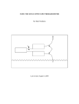
Figure 6: A small region of a spectrum recorded on an SVC HR-1024 spectroradiometer
showing overlapped data (A). The VNIR detector records wavelengths up to
1005 nm whilst the SWIR1 detector starts at 962 nm. When the spectra are
joined (B) at 980 nm a sharp jump in the intensity occurs.
ref =
1x4 struct array with fields:
name
datetime
header
wavelength
data
This separates the target and reference spectra into two separate structure arrays called
tar and ref. Note that the tar structure array has a field called pair which gives the
name of the paired spectrum. This field is used by the relativereflectance function to
calculate reflectance spectra (see Section 4.3.
4.2. Removing overlapped data
Spectroradiometers that cover both the visible near infared (VNIR) and short wave infared
(SWIR) spectral regions have multiple detectors. For example the SVC HR-1024 has a
silicon (Si) array detector for the VNIR spectral region and two indium gallium arsenide
(InGaAs) array detectors for the SWIR region. There is a small area of overlap around
the long wave edge of the Si VNIR detector and the short wave edge of the first InGaAs
SWIR detector (SWIR1). This overlap region is typically in the range 960 − −1050 nm.
Figure 6(A) shows the overlap region in a field spectrum. The overlapped data can cause
problems for processing and must usually be removed prior to any further processing.
On ASD spectroradiometers the overlapped region is removed automatically by the operating software, therefore ASD spectra will never contain overlapped data. On the SVC
HR1024 the overlapped data may be removed or preserved depending on the overlap/matching settings chosen in the SVC operating software (accessed through the
2012-07-18
12
version 1.3.6
4 PROCESSING FUNCTIONS
setup menu)4 . The Facility recommends setting this option to preserve and removing
the overlap during post processing.
A function called removeoverlap is provided in the toolbox to join the VNIR and SWIR1
regions at a specified join wavelength. For example, to remove overlap from target and
reference spectra type by joining the two regions at 980 nm type:
tar_joined = removeoverlap(tar, 980)
ref_joined = removeoverlap(ref, 980)
After joining the spectra there is usually a sharp jump in the spectral data value either
side of the join wavelength. Figure 6(B) shows an example of a spectrum with overlap
removed. This toolbox does not at present provide any ‘matching algorithms’ to remove
this feature.
Note that removing overlapped data changes the set of wavelength values in the spectrum.
The joined spectra will therefore have a different wavelength scale.
4.3. Relative reflectance
Spectral relative reflectance Rrel (λ) as a function of wavelength λ is defined as the ratio of
the target spectrum L(λ) to the corresponding relative reference spectrum Erel (λ)
Rrel (λ) =
L(λ)
Erel (λ)
The relative reflectance spectrum is usually measured in the field by recording a spectrum
of the light reflected from a reference panel.
The function relativereflectance calculates relative reflectance spectra by dividing each
target spectrum by its corresponding reference spectrum. If tar and ref are structure
arrays of paired target and reference spectra, typing:
R_rel = relativereflectance(tar, ref)
calculates relative reflectance spectra. The information about which target spectrum
should be paired with which reference spectrum is contained in the pair field of the target
spectra. Section 4.1 describes how to pair spectra. Note that the number of reflectance
spectra will equal the number of target spectra.
4.4. Absolute reflectance
Absolute spectral reflectance Rabs (λ) as a function of wavelength λ is the ratio of the target
spectrum L(λ) to the spectral irradiance E(λ)
Rabs (λ) =
L(λ)
E(λ)
Generally in field spectroscopy E(λ) is not measured directly, but instead a spectrum of
the irradiance reflected from a reference panel is recorded. What is measured therefore
4
The software used to record spectra on a handheld device (PDA) does not have overlap/matching settings
and preserves overlap by default.
2012-07-18
13
version 1.3.6
4 PROCESSING FUNCTIONS
is the relative irradiance, Erel (λ). This is the spectral irradiance E(λ) multiplied by the
spectral reflectance of the panel Rpanel (λ)
Erel (λ) = Rpanel (λ)E(λ)
If Rpanel (λ) is known, then absolute reflectance can be calculated from the measured relative reflectance
Rabs (λ) =
Rpanel (λ)L(λ)
L(λ)
=
= Rpanel (λ)Rrel (λ)
E(λ)
Erel (λ)
Therefore to convert a measurement of relative reflectance to absolute reflectance the spectrum must be multiplied by the reflectance of the panel that was used to record it. The
panel’s reflectance spectrum, Rpanel (λ), can be measured in the laboratory as a calibration
procedure and the calibration data then applied to field spectra in post processing.
Calibration data for the all Field Spectroscopy Facility’s reference
panels are available in an Excel spreadsheet.
A reference panel calibration spectrum Rpanel (λ) can be imported into MATLAB using
the importpanelcal function. Two file types are supported:
1. A comma-separated values (CSV) file with a header which gives information about
the panel’s calibration
2. An Excel spreadsheet provided by the Field Spectroscopy Facility
An example of a panel calibration file in CSV format is shown in Figure 7. This file can
be used as a template for panel calibration data if required. The header must contain the
panel’s name. This should be a unique name or serial number which identifies which panel
the calibration refers to. The date and time at which the calibration was performed must
also be included in the header.
To import a panel calibration file in CSV format into MATLAB type:
p = importpanelcal(ṕanel.csv´
)
Alternatively, panel calibration data may be imported from an Excel spreadsheet provided
by the Field Spectroscopy Facility. As the spreadsheet contains data for all the Facility’s
panels, the serial number of the panel to be imported must be specified:
P = importpanelcal(F́SF Ref Panel Cal Data 2010_1.xls,́ ŚRT #008´
)
MATLAB will issue a warning when importing data from the FSF’s
Excel spreadsheet to indicate that the xlsread function has limited
import functionality in basic mode. This warning may be safely
ignored.
The panel calibration spectrum can be plotted by typing:
plot(p.wavelength, 100*p.data)
xlabel(’Wavelength nm’)
ylabel(’Panel reflectance %’)
2012-07-18
14
version 1.3.6
4 PROCESSING FUNCTIONS
Figure 7: A example of a CSV file containing a reference panel calibration spectrum. A
copy of this file can be found in the examples folder. It can be imported into
MATLAB with the importpanelcal function. The data consist of wavelengths
in nm and the corresponding panel reflectance as a number in the range 0–1.
2012-07-18
15
version 1.3.6
4 PROCESSING FUNCTIONS
The reflectance values were multiplied by 100 to convert them to per cent.
A structure array of absolute reflectance spectra can be calculated from a structure array
of relative reflectance spectra R_rel and a structure containg the panel calibration data
by typing:
R_abs = absolutereflectance(R_rel, P)
If the panel calibration spectrum was recorded with the same spectrometer as the field spectrum then both will have the same the set of wavelength values (λ). If they were recorded
on different instruments the panel spectrum will be interpolated to the wavelengths of the
relative reflectance spectrum.
Once calculated, the absolute reflectance spectra can be plotted by typing:
plot([R_abs.wavelength], 100*[R_abs.data]);
legend(R_abs.name);
xlabel(’Wavelength (nm)’);
ylabel(’Absolute reflectance (%)’);
title(’Reflectance spectra recorded on SVC GER 1500’);
4.5. Smoothing
Spectra can be smoothed with a Savitzky–Golay filter [6] by typing:
s_smoothed = sgsmooth(s)
This smooths all spectra in the structure array s, returning a structure array of smoothed
spectra s_smoothed.
Note that the smoothing operation reduces the wavelength range of the spectra. The
smoothed spectra will therefore have a different set of wavelength values than the original.
The function sgsmooth makes use of MATLAB’s sgolay function to design the filter. This
function is part of MATLAB’s Signal Processing Toolbox. Further information can be
found in the documentation for sgolay.
4.6. Removing water bands
The solar irradiance reaching the ground can be very low in some spectral regions due to
water absorption. The table below gives two spectral regions where water absorption is
particularly high.
Water band 1
Water band 2
Start wavelength
1350 nm
1790 nm
End wavelength
1460 nm
1960 nm
The high absorption of water results in a very low irradiance E(λ) at ground. As reflection
is divided by irradiance
Rabs (λ) =
L(λ)
E(λ)
the errors transmitted to the absolute reflectance can become very large. This manifests
as noisy regions in spectra. These regions are often ommited from plots.
The function removewater deletes the data points in the above water band regions. Type
2012-07-18
16
version 1.3.6
5 RADIOMETRIC CALIBRATION
30
A
25
Reflectance %
30
20
20
15
15
10
10
5
5
0
500
B
25
1000 1500 2000 2500
Wavelength nm
0
500
1000 1500 2000 2500
Wavelength nm
Figure 8: Example of post processing. The original spectrum (A) contains overlapped data
which were removed with the removeoverlap function. The join wavelength was
980 nm. The spectrum was then smoothed with the sgsmooth function. The
water bands were removed with removewater, resulting in the output spectrum
(B).
s_nowater = removewater(s)
to delete the water bands regions from the structure array s, returning a new structure
array s_nowater. The data points are removed by replacing them with the special value Not
a Number (NaN). This value is commonly used for undefined or unrepresentable numbers.
A more detailed description of NaN is given in the MATLAB documentation.
Figure 8 shows an example of water band removal.
5. Radiometric calibration
For instruments that have been calibrated this section describes how to apply the calibration data to convert reference and target spectra to radiometric (SI) units.
5.1. Introduction
Absolute spectral measurements are those expressed in SI derived units. A calibrated field
spectroradiometer can make measure two key radiometric quantities: spectral radiance
and spectral irradiance. As spectral quantities both are functions of wavelength λ. The
conventional SI units for these quantities are given in the table below:
Quantity
Radiance
Irradiance
Symbol
L(λ)
E(λ)
Units
Wsr−1 m−2 nm−1
Wm−3 nm−1
Calibration standard (typical)
FEL lamp
Integrating sphere lamp
To make absolute measurements the spectroradiometer must first be calibrated, a process
usually performed in the laboratory using a calibrated light source.
All spectrometers measure a spectrum in digital numbers (DN), which must then be converted to the appropriate radiometric quantity by multiplying the spectrum by the system
response for that radiometric quantity5 . The system response measures the signal level
5
The system response is also known as the calibration gain.
2012-07-18
17
version 1.3.6
5 RADIOMETRIC CALIBRATION
at each wavelength to a known source of radiance or irradiance. It depends on many
aspects of the spectroradiometer: the elements in the optical pathway, the properties of
the detectors and the choice fore-optic. For this reason each calibration is specific to a
certain configuration of the spectroradiometer. It must be performed again whenever the
configuration is changed.
5.2. Radiance
Spectral radiance can be calculated by multiplying a measured field spectrum S(λ) in
digital numbers (DN) by the system response to radiance CL (λ)
L(λ) = CL (λ)S(λ)
If CL (λ) is measured in a calibration procedure then any spectrum subsequently recorded
on the same spectroradiometer (in the same configuration) can be expressed as absolute
radiance L(λ) in SI units.
To find CL (λ) a calibration spectrum Scal (λ) is recorded in a carefully-controlled laboratory
setup using a calibrated standard of known radiance Lstandard (λ) as the light source
Lstandard (λ) = CL (λ)Scal (λ)
This equation can be rearranged to find the system repsonse to radiance CL (λ)
CL (λ) =
Lstandard (λ)
Scal (λ)
5.3. Irradiance
Similarly for irradiance, a spectrum can be converted to radiometric units by multiplying
it by the system response to irradiance
E(λ) = CE (λ)S(λ)
Using a known source of irradiance Estandard (λ) the system response to irradiance can be
found
CE (λ) =
Estandard (λ)
Scal (λ)
5.4. Importing the system response into MATLAB
Before calculating radiometric spectra the appropriate system response measurements must
be imported into MATLAB using the importradcal function.
The importradcal function reads calibration data in an XML file format. An example
file in this XML format is provided in the examples folder. This folder is located in
the FSFPostProcessing1.3.6 folder at the location where the toolbox was installed. A
template for Microsoft Excel is also provided to read and write files in this format. The
template can be found in the excel folder.
2012-07-18
18
version 1.3.6
6 COMPARISON WITH AIRBORNE AND SATELLITE INSTRUMENTS
Radiometric calibration data for calibrations performed at the
Field Spectroscopy Facility are available in an Excel spreadsheet.
MATLAB cannot import this spreadsheet directly. The data set
for the instrument used must exported to an XML file using the
provided Excel template.
To import a radiometric calibration XML file
C_L = importradcalŕadcalexample.xml´
)
The data file is imported into a structure array. If output is not suppressed (with a semicolon at the end of the line) then the structure is displayed
C_L =
name: ’FSF radiance calibration example’
datetime: ’27-Oct-2009 12:00:00’
header: [1x1 struct]
wavelength: [2151x1 double]
data: [2151x1 double]
The wavelength and data fields give the system response measurement at each wavelength.
The header field provides additional information (imported from the XML file) about the
calibration such as the instrument’s serial number and the calibration standard which was
used to measure the system response.
5.5. Calculating radiance and irradiance
If S is a structure array of target field spectra and C_L is the system response imported
with the importradcal function then radiance can be calculated by typing:
L = radiance(S, C_L)
Similarly, if S is a structure array of reference field spectra and C_E is the system response
to irradiance then irradiance can be calculated by typing:
E = irradiance(S, C_E)
Although the radiance and irradiance functions perform exactly
the same calculation they should be applied to different types of
spectra and give results in different units.
6. Comparison with airborne and satellite instruments
This section describes the convolve function which can be used to reduce the spectral
resolution of field spectra to match the bands of a airborne or satellite instrument. A Band
class is also introduced which provides a convenient way to load, store and plot the spectral
response functions of these instruments in MATLAB.
2012-07-18
19
version 1.3.6
6 COMPARISON WITH AIRBORNE AND SATELLITE INSTRUMENTS
6.1. Introduction
The need often arises to compare field spectra with spectra recorded by airborne or satellite
spectroscopic instruments such as imaging spectrometers. These instruments typically have
poorer (or much poorer) spectral resolution than field spectrometers and will therefore
provide less detailed spectra. In order to make a sensible comparison the spectral resolution
of the field spectra must be reduced to match the spectral response functions (bands) of
the airborne or satellite instruments. This is done by convolving the field spectra with the
response functions.
The types of instruments fall into two broad classes: multispectral imagers and imaging
spectrometers6 . The convolution process is different for the two instrument types and will
be described in separate subsections.
6.2. Multispectral instruments
The spectral response function of an instrument describes the spectrum produced by the
detector in response to a purely monochromatic light source at a wavelength λsource [7].
Multispectral sensors make measurements of light ’intensity’ in a number different bands.
The spectral response function of each band therefore describes the response of the band’s
detector to monochromatic light at wavelength λsource . For an instrument with N bands,
the response of band n to a monochromatic light source at wavelength λsource is given by
a function fn (λsource ). As each band has its own spectral response function, there will be
a set of such functions
f1 (λsource ), f2 (λsource ), ..., fN (λsource )
In general it is not important to know the absolute spectral response of an instrument and
the relative spectral response is sufficient. The functions are therefore normalized to unit
area
ˆ ∞
fn (λ)dλ = 1 for all n
0
If the source spectrum Ssource (λ) were known—which it generally isn’t—the total response
in band n could be found by integrating the product of the source spectrum and the
spectral response function over the full range of wavelengths λ
ˆ ∞
Sn =
Ssource (λ)fn (λ)dλ
0
Often it is required to calculate the relative band responses that would be generated if a
known field spectrum were detected by a multiband detector. In this scenario the highresolution field spectrum can be assumed to be identical with the source spectrum and
substituted for it in the above equation to give
ˆ
Sn =
∞
Sf ield (λ)fn (λ)dλ
0
6
Imaging spectrometers are also known as hyperspectral instruments.
2012-07-18
20
version 1.3.6
6 COMPARISON WITH AIRBORNE AND SATELLITE INSTRUMENTS
The set of spectral response functions fn (λsource ) is typically measured as part of the instrument’s calibration. Armed with this measurement, and the field spectrum Sfield (λ), the
above integral can be calculated. The discrete measurements are multiplied (interpolating
if necessary) and the integral is performed with an approximation method such as the
trapezoidal rule.
It is common to label the bands not by their index n, but by their centre wavelengths λc .
6.3. Spectrometers
A spectrometer has a set of closely-spaced spectral response functions which depend on
the source wavelength λsource . The response of the instrument at detector wavelength λ to
a purely monochromatic light source at wavelength λsource has the functional form
f = f (λ, λsource )
It is common to assume—and usually the case [7]—that the shape of f changes only slightly
with source wavelength. It can therefore be expressed as a single function shifted to the
source wavelength
f = f (λ − λsource )
Again, the spectral response function is generally normalized such that
ˆ ∞
f (λ)dλ = 1
−∞
The detected spectrum is the response at detector wavelength λ due to light from all parts
of the source spectrum is found by integrating over all the source wavelengths
ˆ ∞
S(λ) =
Ssource (λsource )f (λ − λsource )dλsource
0
This integral is the convolution of the source spectrum with the spectral response function.
The result is the detected spectrum as a function of wavelength S(λ).
Ideally the spectral response function of every instrument would be measured. In practice
this may not be possible and a variety of methods have been developed to approximate it
[8]. These generally involve approximating the spectral response functions as a series of
Gaussian functions whose widths and centre wavelengths are set up to match the instrument’s specifications.
6.4. Reducing the spectral resolution
For comparing spectra of high resolution (HR) ground-based field spectrometers with the
comparitavely lower resolution (LR) airborne or satellite instruments the HR data must
be reduced in resolution to the LR instrument. In other words we wish to know how a
particular spectrum acquired on the ground would appear if it had been detected with
a lower resolution instrument. This question can be answered by convolving the source
spectrum with the spectral response function of the LR instrument
ˆ ∞
SLR (λ) =
Ssource (λsource )fLR (λ − λsource )dλsource
0
2012-07-18
21
version 1.3.6
6 COMPARISON WITH AIRBORNE AND SATELLITE INSTRUMENTS
Unfortunately the source spectrum is not usually known. However, if the HR instrument
has a spectral resolution significantly higher than the LR instrument, its spectral response
funciton may be sufficiently narrow that the source spectrum can be approximated by the
HR spectrum
SHR (λ) ≈ Ssource (λ)
Substituting into the above equation
ˆ ∞
SHR (λsource )fLR (λ − λsource )dλsource
SLR (λ) =
0
If fLR is known or modelled then this convolution can be performed numerically.
6.5. In MATLAB
The function convolve provides a means to convolve a spectrum or spectra with the
spectral response functions of a specific airborne or satellite instruments. The first step
in this processing function is to download the spectral response functions (bands) for the
specific instrument. A MATLAB class called Band is provided to facilitate handling these
data. A class works in a very similar way to a structure array, however classes can also
contain methods. An introduction to classes is given in the MATLAB documentation.
A selction of band data for various instruments is available from
the Field Spectroscopy Facility’s web site.
These data are provided as XML files and are listed on the Field
Spectroscopy Facility’s web site.
The class Band can be used to load response data into MATLAB. For example, to load
spectral response data for the POLDER instrument type
POLDER = Band(’http://fsf.nerc.ac.uk/user_group/bands/POLDER.xml’)
This loads the data into MATLAB and stores it in an object called POLDER. To plot the
bands type:
POLDER.plot
By default the spectral response functions are are normalized to unit area. The normalizeHeight
method can be used to normalize such that the height of each response function is 1:
POLDER.normalizeHeight.plot
To convolve a field spectrum in a structure array S with the spectral bands, type
t = convolve(s, POLDER)
If the spectrum S and the bands POLDER are defined on different wavelength scales, the
bands will be interpolated. The colvolved spectra will be output in a structure array t.
If the band centre wavelengths have been defined the output spectrum can be plotted by
typing:
plot(t.wavelength, t.data)
2012-07-18
22
version 1.3.6
A NORMALIZATION OF ASD SPECTRA IN RAW MODE
6.6. Feature depth estimation
The depth of an absorption feature in a spectrum can be estimated using the method
described by Clark and Roush [9]. The function featuredepth provides an illustration of
the method. If s is a spectrum, the depth of an absorption feature between wavelengths
w1 and w2 can be estimated by typing:
[wf, depth] = featuredepth(s, w1, w2)
The output wf gives the wavelength of the feature. The funciton also plots an illustration
of the process used to estimate the depth.
References
[1] Milton, Edward J., “Progress in field spectroscopy,” Remote Sensing of Environment,
volume 113, pp. S92–S109, 2009
[2] Spectra Vista Corporation, HR-1024 User Manual, 1.5 edition, 2008
[3] MacLellan, Chris J. and Malthus, Tim J., “High performance dual field of view spectroradiometer with novel input optics for autonomous reflectance measurements over
an extended spectral range,” IGARSS, 2009
[4] Robinson, Iain and MacLellan, Chris J., “A dual field of view spectroradiometer for
near-simultaneous measurement of irradiance and reflected radiance,” , 2011
[5] MacLellan, C., V–SWIR data file format and remote control command set, Field Spectroscopy Facility, 7 edition, 2010
[6] Savitzky, Abraham and Golay, M J E, “Smoothing and Differentiation of Data by
Simplified Least Squares Procedures.” Analytical Chemistry, volume 36, no. 8, pp. 1627–
1639, 1964
[7] James, J F, Spectrograph Design Fundamentals, Cambridge University Press, 2007
[8] Milton, E. J. and Choi, K. Y., “Estimating the spectral response function of the CASI2,” Proceedings of the Annual Conference of the Remote Sensing and Photogrammetry
Society, 2004
[9] Clark, R N and Roush, T L, “Reflectance spectroscopy: quantitative analysis techniques
for remote sensing applications,” J Geophys Res, volume 89, p. 6329, 1984
A. Normalization of ASD spectra in raw mode
ASD spectra recorded in raw mode must be normalized to account for the different responses of the detectors. The normalization is performed during import and the code is
contained in the function ASDFieldSpec. (Reflectance spectra recorded in white reference
mode are not normalized.)
The ASD FieldSpec 3 and FieldSpec Pro spectroradiometers have three separate detectors
for three different spectral regions. A silicon photodiode array detects light in the visiblenear-infrared (VNIR) region. Two InGaAs photodiodes cover two short wave infrared
spectral regions labelled SWIR1 and SWIR2.
2012-07-18
23
version 1.3.6
A NORMALIZATION OF ASD SPECTRA IN RAW MODE
VNIR
SWIR1
SWIR2
λ1 and λ2 are the join wavelengths. These may be different for different instruments, but
the values are saved in ASD spectrum files. They can be found in the header structure in
fields named Join1Wavelength and Join2Wavelength.
The pixel values DN are normalized differently in each spectral region:
 DN(λ)
λ 6 λ1

 TVNIR
GSWIR1 DN(λ)
DNnorm (λ) =
λ1 < λ 6 λ2
2048

 GSWIR2 DN(λ)
λ2 < λ
2048
where TVNIR is the integration time of the VNIR photodiode array, GSWIR1 is the gain of
the SWIR1 photodiode and GSWIR2 is the gain of the SWIR2 photodiode. These values are
saved in ASD spectrum files, and are imported into the MATLAB workspace as fields in the
header structure called VNIRIntegrationTime, SWIR1Gain and SWIR2Gain respectively.
2012-07-18
24
version 1.3.6
B. Using ViewSpec Pro to Convert ASD Binary
Files to ASCII
The application ViewSpec Pro from ASD includes many useful features such as
graphing, scaling, 1st derivative and conversion of the spectrometer’s binary files
into ASCII text files. For the purpose of this guideline we will only use the ASCII
Export function. The application is installed on each of the facility’s computers and
is also available for the Analytical Spectral Device’s website ftp://ftp.asdi.com/Software/
contact FSF for further details.
•
Start the ViewSpec Pro application.
Configuring ViewSpec Pro
The application can save the path/directory to your ASD spectrum files and the
converted text files.
•
From the Setup menu click on the Input Directory to select a New Directory
Path to your ASD binary data files.
After selecting the default Input Directory you are offered the opportunity to make
the Output Directory match the Input Directory. Alternatively, you can select a
different path/directory using the Setup /Output Directory menu.
Open ASD Spectrum (Binary) Files
ViewSpec Pro can open and process large numbers of files although graphing is
limited to 14 spectra.
•
From the File menu select Open and highlight the ASD White-Ref or radiometric
binary files for importation.
•
Click Open to bring the files into ViewSpec Pro.
Converting ASD Binary Files to ASCII text
The file list is shown in the application window.
•
Highlight each file in the list.
•
From the Process menu select ASCII Export.
•
Ensure the boxes/buttons circled in red are selected.
•
* NOTE The new ASD ViewSpec Pro software allows different data formats and
derivatives to be selected if required – see the dialogue box below. ‘DN’ and
derivative - ‘none’ are recommended.
•
Click OK to convert the files to ASCII and save them in the Output directory.
•
Close the ViewSpec Pro application.
* If using the old version of
ViewSpec
Pro
(4.05)
the
additional data formats are not
available and the box will look like
this.