Download Iterative Learning Control for a Reluctance Actuator

Iterative Learning Control
for a Reluctance Actuator
G.M. Heldens
CST 2010.071
Master traineeship report
Coach:
[FIT] Associate Professor; H. Gutiérrez Ph.D. (Héctor)
Supervisor: [TUe] Prof. Dr. Ir. M. Steinbuch (Maarten)
Eindhoven University of Technology
Department of Mechanical Engineering
Control Systems Technology group
Eindhoven, November 2010
Abstract
In this research the performance of a Hybrid Magnetic Suspension Actuator (HMSA) is investigated. The reluctance actuator has a long range (1 [mm]) and a high accuracy (submicrometer). Permanent magnets are used to compensate for gravitational forces. The big
advantages of this type of actuator is the long range, high accuracy and that the force on the
load is transferred contact less. This implies that it does not need any guidance system (for
example with air bearings). Which makes the actuator suitable for vacuum conditions. The
permanent magnets reduce the current needed to levitate the load, to reduce heat dissipation
in the system.
A 1-DOF setup is used to test several control strategies for the actuator. The system is nonlinear and non-affine in the input. A new control system is used, and previously designed
controllers are transferred to the new hardware platform. The parameters of the system are
estimated again and the performance is compared with the old hardware performance. The
previously designed controllers were a PID-controller and a non-affine sliding mode controller.
To improve the performance, an Iterative Learning Controller (ILC) is designed. The feedforward signal of the ILC is calculated using multiple learning filters, due to the fact that the
system is non-linear. The reference value is used to select the corresponding learning filter.
Before applying the discontinuous feedforward signal, the signal is smoothed with a filter.
Furthermore simulations are done for a 6-DOF setup, to prove that ILC also has a positive
effect on this MIMO-system.
i
Samenvatting
In dit onderzoek worden de prestaties van een ’Hybrid Magnetic Suspension Actuator’ (HMSA)
onderzocht. De actuator heeft een groot bereik (1 [mm]) en een hoge nauwkeurigheid (submicrometer). Permanente magneten worden gebruikt om de zwaartekracht te compenseren.
Het grote voordeel van dit type actuator is het grote bereik, de hoge nauwkeurigheid en dat
de krachten op de te actueren massa contactloos worden overgedragen. Hierdoor hoeft er geen
gebruik gemaakt te wordt van een geleiding met lucht lagers. Dit maakt het systeem geschikt
voor vacuüm toepassingen. De permanente magneten reduceren de benodigde stroom door de
spoel om de te positioneren massa te laten zweven. Dit reduceert de warmte productie in het
systeem.
Een 1-DOF setup is gebruikt om verschillende controller strategieën te testen voor deze actuator. Het systeem is niet-lineair en de ingang is ’non-affine’. Een nieuw hardware platform is
geïnstalleerd en de in het vorig onderzoek ontworpen controllers zijn overgezet naar het nieuwe
systeem. De systeem parameters zijn opnieuw bepaald en de prestaties zijn vergeleken. De
vorige controllers waren een PID-controller en een ’non-affine sliding mode’-controller.
Om de prestaties te verhogen is voor beide controllers een iteratief leer algoritme (Iterative
Learning Control - ILC) ontworpen. Het feedforward signaal van het ILC algoritme wordt
berekend door gebruik te maken van verschillende leer filters, omdat het systeem niet-linear
is. De referentie waarde wordt gebruikt om de juiste leer filter te selecteren. Voordat het niet
continue feedforward signaal wordt toegepast, wordt het gesmooth met een filter. Verder zijn
er ook simulaties gedaan voor een 6-DOF setup, om te bewijzen dat ILC ook een positieve
invloed heeft op de prestaties van dit soort MIMO-systemen.
ii
Preface
This internship at the Florida Institute of Technology (FIT) is part of my Master studies
Mechanical Engineering at the Eindhoven University of Technology (TU/e). Within the department of Mechanical Engineering I am following the track Control Systems Technology. For
this internship I spend three months in the Dynamic Systems and Mechatronics lab in Melbourne, Florida, USA. Although three months were too short to fully complete my assignment,
I have learned a lot and gained a lot of ’hands on’ and hardware experience.
Acknowledgments
My coach Héctor Gutiérrez (FIT) was really enthusiastic about the project. He gave me the
freedom to choose which way to go with the research, and he he motivated and stimulated me
to investigate new options all the time. He guided me through the internship and his efforts
paid off: I have learned a lot during these months and I am very thankful he helped me with
that.
Also the people in the lab and the persons I met in Melbourne contributed to my pleasant
stay and my social life outside the office hours. I really want to thank them for guiding me in
the first weeks and becoming my friends.
iii
Table of Contents
Abstract
i
Samenvatting
ii
Preface
iii
Table of Contents
iv
1 Introduction
1.1 Literature . . . . . . . . . . . . . . . . . . . . . . . . . . . . . . . . . . . . . . .
1.2 General overview HMSA . . . . . . . . . . . . . . . . . . . . . . . . . . . . . . .
2 One Degree of Freedom
2.1 Mechanical overview . . . . . . . . . . . . .
2.1.1 Elastic beam . . . . . . . . . . . . .
2.1.2 Hardware . . . . . . . . . . . . . . .
2.2 Modeling . . . . . . . . . . . . . . . . . . .
2.3 Nonlinear observer . . . . . . . . . . . . . .
2.4 Feedback linearization . . . . . . . . . . . .
2.4.1 Parameter estimation . . . . . . . .
2.5 Control strategies . . . . . . . . . . . . . . .
2.5.1 PID . . . . . . . . . . . . . . . . . .
2.5.2 Non-affine sliding mode . . . . . . .
2.6 Iterative learning control . . . . . . . . . . .
2.6.1 System identification . . . . . . . . .
2.6.2 Repetitive and non-repetitive errors
2.6.3 Discontinuous ILC . . . . . . . . . .
2.6.4 Results . . . . . . . . . . . . . . . .
.
.
.
.
.
.
.
.
.
.
.
.
.
.
.
.
.
.
.
.
.
.
.
.
.
.
.
.
.
.
.
.
.
.
.
.
.
.
.
.
.
.
.
.
.
.
.
.
.
.
.
.
.
.
.
.
.
.
.
.
.
.
.
.
.
.
.
.
.
.
.
.
.
.
.
.
.
.
.
.
.
.
.
.
.
.
.
.
.
.
.
.
.
.
.
.
.
.
.
.
.
.
.
.
.
.
.
.
.
.
.
.
.
.
.
.
.
.
.
.
.
.
.
.
.
.
.
.
.
.
.
.
.
.
.
.
.
.
.
.
.
.
.
.
.
.
.
.
.
.
.
.
.
.
.
.
.
.
.
.
.
.
.
.
.
.
.
.
.
.
.
.
.
.
.
.
.
.
.
.
.
.
.
.
.
.
.
.
.
.
.
.
.
.
.
.
.
.
.
.
.
.
.
.
.
.
.
.
.
.
.
.
.
.
.
.
.
.
.
.
.
.
.
.
.
.
.
.
.
.
.
.
.
.
.
.
.
.
.
.
.
.
.
.
.
.
.
.
.
.
.
.
.
.
.
.
.
.
.
.
.
.
.
.
.
.
.
.
.
.
.
.
.
.
.
.
.
.
.
.
.
.
.
.
.
.
.
.
.
.
.
.
.
.
.
.
.
.
.
.
1
1
1
3
3
3
4
4
5
5
6
6
7
8
10
13
13
14
14
3 Six Degrees of Freedom
17
3.1 Iterative learning control . . . . . . . . . . . . . . . . . . . . . . . . . . . . . . . 18
4 Conclusion and Recommendations
19
4.1 Conclusion . . . . . . . . . . . . . . . . . . . . . . . . . . . . . . . . . . . . . . . 19
4.2 Recommendations . . . . . . . . . . . . . . . . . . . . . . . . . . . . . . . . . . 19
References
21
iv
TABLE OF CONTENTS
A Nomenclature
v
23
B Installing the Speedgoat
24
B.1 IO-cards . . . . . . . . . . . . . . . . . . . . . . . . . . . . . . . . . . . . . . . . 24
B.2 Installation . . . . . . . . . . . . . . . . . . . . . . . . . . . . . . . . . . . . . . 25
B.3 Tips and tricks . . . . . . . . . . . . . . . . . . . . . . . . . . . . . . . . . . . . 27
C Load cell calibration
29
D Simulink schemes
31
E Graphs ILC
33
Chapter 1
Introduction
For al long time, technology tends towards the development of smaller components. As a
reaction on this, the high-precision manufacturing industry is continuously pushing the limits
of the positioning accuracy from the actuators used. Magnetic Servo Levitation (MSL) is a
tried and known concept, however, it is currently not being applied much in high accuracy
positioning systems. Advantages of MSL-actuators are the high accuracy, high bandwidth and
frictionless load transfer (no physical contact). Another big advantage is that the actuator
can operate in vacuum. The semiconductor industry is hitting a physical boundary in the
lithography process, due to the air molecules present in the machine. This makes a MSLactuator the suitable candidate for the high demanding specifications of a wafer stage in
vacuum.
1.1
Literature
The actuator used in this research is a Hybrid Magnetic Suspension Actuator (HMSA). The
first 6-DOF concept was designed by L. Fevre [1], where E. Visser [2] improved the control
strategy. In 2005 J. Simons and N. Kleijn [3] further improved the 6-DOF actuator performance by redesigning the electromagnet and made a 1-DOF setup for the actuator characterization. D. Li [4] completely redesigned the 6-DOF actuator stage. Finally J.J. Bolder [5]
demonstrated an improvement in performance by applying a non-affine sliding mode controller
on the 1-DOF setup.
1.2
General overview HMSA
When using Magnetic Servo Levitation only electromagnetic coils are used to compensate
the gravity force. In the MSL-actuator a lot of current is needed to generate a force against
gravity. The current in the coils heats up the complete actuator, causing it to lose accuracy.
When permanent magnets are use to support the mass against gravity, less current is needed.
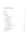
This type of actuator is called a Hybrid Magnetic Suspension Actuator (HMSA). In Figure
1.1 a schematic overview shows the permanent neodymium (NdFeB) magnets in the actuator
1
1.2 General overview HMSA
2
as well in the target with opposing faces.
Ferromagnetic Face
g
Permanent
Magnets
Permanent
Magnet Sleeve
Electromagnetic
Coils
Sleeve
Bobbin
Lead Screw
Figure 1.1: Schematic HMSA (adapted from [4]).
To use the actuator, the target has to be pulled a little bit to the electromagnetic coils. This
is because the coil can only attract the target by shortening the magnetic field lines. The
coil is unable to repel the target. The force of the permanent magnets is used to move the
target away from the coils. With the lead screw the passive floating hight of the target can
be adjusted. Most of the magnetic field is contained in the steel sleeve around the coils. This
is to avoid scattering of the field and to avoid non-axial forces on the target. The goal of this
research is to achieve a long range travel (1 [mm]) with sub-micrometer accuracy.
Chapter 2
One Degree of Freedom
To test the tracking performance of the actuator and to test some control strategies a 1-DOF
setup is used.
2.1
Mechanical overview
The setup used consist of an elastic beam, actuated by a HMSA-actuator. The current to
the actuator is supplied by a current amplifier, which is controlled by a control system. The
position of the beam is measured by a capacitive sensor. The used hardware will be discussed
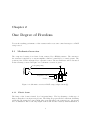
in the following sections. In Figure 2.1 a schematic overview is given.
Leaf-spring hinge
F
x1
Capacitive sensor
Actuator
u
Figure 2.1: Schematic overview 1-DOF setup (adapted from [5]).
2.1.1
Elastic beam
The hinge of the beam is formed by a leaf-spring hinge. The big advantage of this type of
hinge is that there is no hysteresis present. Two bump stops prevent the beam from deforming
plastically. By giving the beam a slight offset perpendicular to the actuator force, the gravity
force is simulated. Due to the long length of the beam and the relatively small translation, a
3
2.2 Modeling
4
pure translation at the end of the beam can be assumed. In the side of the beam a steel face
with the opposing magnets is mounted as a target for the actuator.
2.1.2
Hardware
The other hardware, besides the beam setup, consists of a sensor, current amplifiers, filters
and the control system. The sensor used is a capacitive sensor from Lion precision, model
C14-K. There is a high and a low sensitivity range available. In the low sensitivity mode the
measurement range is from 500 to 1500 [µm], with a bandwidth of 100 [Hz] and an accuracy
of 60 [nm]. In the high sensitivity mode, the range is from 950 − 1050 [µm], with a bandwidth
of 20 [kHz] and an resolution of 4 [nm]. The measurement noise in the test setup is approximately 80 [nm] in low sensitivity mode.
The used current amplifier is a 25A20 Pulse Width Modulation (PWM) servo controller from
advanced motion controls, with a bandwidth of 190 [Hz]. The output from the amplifier is
filtered to create a smooth, non pulsing output. The coil current typically varies between 0
and 2.5 [A].
The used control system is a real-time target machine from speedgoat in combination with the
xPC target toolbox from Matlab. The big advantage of this system is the integrated design
of the control strategies in Simulink, with simulations and hardware in-the-loop tests. The
Real-time target is able to run at least at 25 [kHz] with the used input and output cards.
The previous research was done with another control system with a sampling frequency of 2.5
[kHz]. To compare results the real-time target is also used at the same sampling frequency.
In Appendix B an installation guide can be found.
2.2
Modeling
The plant is a single input single output system with position as output and current as input.
The permanent magnets exert a force which is quadratic as a function of the position, but in
the working range this force can be modeled linear, according to [3]. The model of the plant
is adapted from [6] and is described by Equation (2.1). In this equation x1 is the position and
x2 is the velocity of the beam, m is the translational mass of the beam. The parameters k1
and k2 are the lumped stiffness of the beam and the permanent magnets and c is the damping.
x=
x1
x2
,
f (x) =
B =
ẋ = f (x) + Bh(u, x1 )
f1 (x)
f2 (x)
0
m−1
=
,
with:
x2
m−1 (−k1 x1 + k2 − cx2 )
h(u, x1 ) = −
k3 u2
(x1 + go )2
(2.1)
,
2.3 Nonlinear observer
5
The force of the coil on the beam is described by h(u, x1 ), the nominal gap between beam and
coil is given by g0 . And the force is quadratic with respect to the current through the coil (u),
but it is also quadratic with respect to the gap between coil and beam.
2.3
Nonlinear observer
The velocity of the beam is necessary to be able to control the system. Only the position of
the beam in the test setup is measured, so the velocity has to be extracted by differentiating
the position. Because the position signal is noisy, the velocity estimation is very unreliable.
To reconstruct all the states a nonlinear observer is used. Due to the fact that the observer
filters noise from the feedback signal, the closed loop behavior will be improved. The nonlinear
observer from [5] will be implemented. The general form of the observer can be seen in (2.2),
in which x̂˙ is the observed state.
(2.2)
ẋ = Nx + g(u, y)
y = Cx
with:
0
0
1
−1
,
, g(u, y) = m
N =
k2 + h(u, y)
−m−1 k1 −m−1 c
1 0 , y = x1 .
C =
The full state of the system can be reconstructed, because the pair (N, C) is observable.
Because the function g(u, y) is not exactly known, an asymptotically and robust observer has
to be designed. The observer is formulated in Equation (2.3). By designing H1 such that
N − H1 C is Hurwitz, the observer error is asymptotically stable [7].
x̂˙ = Nx̂ + g(u, y) + H1 (y − Cx̂)
(2.3)
To make the observer robust against model errors a high gain observer is designed [7]. This
can be done by adding integration of the observer error to the state estimation. The final
observer can be seen in Equation (2.4). By choosing high values for H2 , the observer is robust
against mode errors. This is shown in experiments and in simulations by [5].
x̂˙ = Nx̂ + g(u, y) + H1 (y − Cx̂) + H2
Z
t
(y − Cx̂)dt
(2.4)
0
2.4
Feedback linearization
The most common approach for control of magnetic systems is applying feedback linearization
(FL) in combination with linear control techniques. The derivation of the full state linearization can be found in [5]. As shown in the paper, the system is fully feedback linearizable, so
2.5 Control strategies
6
no dynamics remain after the transformation. The transformation to apply on the input u0 is
shown in Equation (2.5).
s
u=
2.4.1
(x1 + g0 )2
(−k1 x1 + k2 − cx2 − u0 )
k3
(2.5)
Parameter estimation
To apply the feedback linearization and to be able to do simulations, the model parameters
have to be determined. To do this a load cell is attached to the beam. With this load cell the
netto force on the beam from the permanent magnets and the coil is measured. To determine
the parameters (k1 , k2 , k3 and x0 ) the current through the coil and the gap between the bar
and the sensor are varied. By solving the object function in Equation (2.6), the parameters
can be extracted with a nonlinear multidimensional optimization algorithm. Before testing
the load cell has to be calibrated. See Appendix C on page 29 for details.
min
X
F m − −k1 x1 + k2 −
k3 u2
(x1 + g0 )2
2
(2.6)
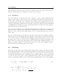
In Figure 2.2 (a) the optimized object function can be seen. Figure 2.2 (b) shows the error
between the estimated parameters and the measured data.
40
20
Force [N]
0
−20
−40
−60
−80
1.5
1
−3
x 10
0.5
Absolute Gap [µ m]
3
2.5
2
1.5
1
0.5
0
Coil Current I [A]
(a) Minimized object function
(b) Error between estimations and measurements.
Figure 2.2: Force, Current and Gap relationship in the actuator.
2.5
Control strategies
Three types of controllers are investigated in previous research: PID, sliding mode and nonaffine sliding mode control. A short description of all strategies is given, including a plot of
2.5 Control strategies
7
the realized performance. The goal is not to improve the tracking error, but checking if there
are errors from translating the C-code used previously on the Digital Signal Processor (DSP)
to the Simulink files in combination with the real-time target (xPC). The final goal of this
research is implementing Iterative Learning Control in which the performance of the controller
is less important for showing the proof of concept.
2.5.1
PID
The PID controller is designed with loop shaping. This controller was used in the previous research to make a comparison between the sliding mode and non-affine sliding mode controllers.
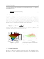
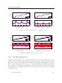
Three types of test are performed to determine the performance. In Figure 2.3 a sinusoidal
signal with different amplitudes and a frequency of 1 Hz is used as a reference signal. With an
amplitude of 500 µm the full range of the beam is reached. As can be seen in Figure 2.3 (a),
the error of the controlled system goes up dramatically at high amplitudes. This behavior can
be explained by the fact that the controller can not track the reference and the beam hits a
bump stop. The plotted values are root-mean-square (RMS) values of the error, captured for
three complete periods.
40
40
DSP
xPC
30
30
25
25
20
15
20
15
10
10
5
5
0
0
100
DSP
xPC
35
RMS error [µm]
RMS error [µm]
35
200
300
Reference amplitude [µm]
(a) PID-controller.
400
500
0
0
100
200
300
Reference amplitude [µm]
400
500
(b) Non-affine sliding mode controller.
Figure 2.3: RMS-error for tracking a sinusoidal reference.
In Figure 2.4 and 2.5 a staircase reference is used. A third order reference is used. This
reference is preferred above a real step in the reference position, because this excites highfrequent and unmodeled dynamics. Besides that, the reference signal is three times continuous
differentiable. In the reference signal two different step heights are used. In Figure 2.4, the
step height is 100 µm. Figure 2.5 shows a staircase profile with ∆ref = 5 µm. As can be seen
the errors of the DSP and the xPC are in the same order of magnitude. Besides that, the
shape of the error is the same. The slightly better performance for the staircase reference with
∆ref = 100 µm can be explained by a slightly different parameter estimation. The controller
parameters used are the same. In Figure 2.5 (a) can be seen that the amplitude of the error is
equal, but the error of the DSP has a slight offset. A schematic overview of the used Simulink
scheme can be seen in Figure D.3 on page 32.
2.5 Control strategies
8
1300
Position [µm]
Position [µm]
1300
1200
1100
DSP
xPC
1000
0
0.5
1
1.5
2
2.5
1200
1100
3
0
0.5
1
1.5
2
2.5
3
0
0.5
1
1.5
Time [s]
2
2.5
3
10
Error [µm]
Error [µm]
10
5
0
−5
DSP
xPC
1000
0
0.5
1
1.5
Time [s]
2
2.5
5
0
−5
3
(a) PID-controller.
(b) Non-affine sliding mode controller.
1235
1235
1230
1230
1225
1220
DSP
xPC
Ref.
1215
1210
1205
0
0.5
1
1.5
2
2.5
3
3.5
1225
1220
DSP
xPC
Ref.
1215
1210
1205
4
1
1
0.5
0.5
Error [µm]
Error [µm]
Position [µm]
Position [µm]
Figure 2.4: Staircase reference, ∆ref = 100 µm.
0
−0.5
−1
0
0.5
1
1.5
2
2.5
3
3.5
4
0
0.5
1
1.5
2
Time [s]
2.5
3
3.5
4
0
−0.5
−1
0
0.5
1
1.5
2
Time [s]
2.5
3
3.5
(a) PID-controller.
4
(b) Non-affine sliding mode controller.
Figure 2.5: Staircase reference, ∆ref = 5 µm.
2.5.2
Non-affine sliding mode
The other control strategy used is a non-affine sliding mode controller. Sliding mode control
(SMC) is suitable when there are parametric and unstructured uncertainties in the model of the
plant. The controller deals with these uncertainties by applying a discontinuous control law.
The nth order control problem is reduced to a first order stabilization problem [8]. Standard
SMC controllers only work for systems that are affine in the input. In the previous research
[5] implemented a non-affine SMC-controller also used in [9] for the control of a non-affine
system of the form:
ẋ = f (x) + Bh(u, x).
(2.7)
2.5 Control strategies
9
The control effort used to control the system consists of two parts: u = us + ueq , with us the
switching control effort and ueq the equivalent control effort. The switching control stabilizes
the system and makes the controle loop robust against disturbances. The equivalent control
reduces chattering, caused by the switching control, as described in [8]. Here a short overview
of the used non-affine SMC-controller can be found. For an extended description see: [5].
Switching control
The one-dimensional, ith order surface will be referred to as the sliding surface. The goal of
the controller is to maintain s = 0 in Equation (2.9). The variable of interest in the equation
is x1 − r. The integral action compensates for slow varying disturbances. When s = 0, the
nth order tracking problem reduces to a first order stabilization problem of the dynamics at
the surface. In order to function, the sliding surface must be attractive and an invariant set.
The third order sliding surface is defined as:
Z t
2
(x1 − r)dt,
s = (x2 − ṙ) + 2λ(x1 − r) + λ
(2.8)
0
with the following modified surface reaching law:
(2.9)
sṡ < 0.
The following sliding condition is found:
s∗ = (h(u, y) + ρ(x)) < 0
∗
∗
with:
(2.10)
−1
= Ds ⇔ s = s D ,
δs
D =
B,
δx δs
δs
−1
ρ(s) = D
+
.
δxf
δt
s
There are two possible cases for the switching control law: s > 0 and s < 0. The control
action must always satisfy the sliding condition in (2.10). After substitution for s > 0, the
proposed control law yields:
s
(x1 + g0 )2
us (t, x) =
n(x), n(x) = k|ρ(x)|, k ≥ 1.
(2.11)
k3
For s < 0 to hold, (h(u, y) + ρ(x)) < 0 must be satisfied as can be seen in Equation (2.10).
With input function:
h(u, y) = −
k3 u(t)2
≤ 0,
(x1 + g0 )2
(2.12)
it yields that us (t) = 0. To guarantee attractiveness of the sliding surface, it must hold that:
ρ(x) > 0. After some algebra if follows that:
ẋ2 + 2λx2 + λ2 x1 > r̈ + 2λṙ + λ2 r.
(2.13)
2.6 Iterative learning control
10
This shows that the reference trajectory must satisfy the restrictions posed in (2.13), to
guarantee attractiveness (so s = 0). The physical interpretation of this equation when s < 0
is that the reference should change slower than the maximum rate of change allowed by the
beam dynamics. The maximum allowable speed of the beam is proportionally to the total
potential energy available in the system. The potential energy consists of the stiffness of the
beam and the load of the permanent magnets
Equivalent control
The switching control introduces chattering due to the pure switching action. Equivalent
control (ueq ) reduces the chattering by driving the system once the sliding surface has been
reached. To derive ueq , the following equation is solved:
ṡ =
δs
δs
+
(f (x) + Bh(u, y)) = 0,
δt δx
solving for u yields:
r
m
ueq (t, x) =
ρ(x)(g0 + x1 )2 .
k3
(2.14)
(2.15)
To guarantee existence and to comply with the sliding condition (2.10):
ueq (t, x) = 0 if (s < 0) ∨ (ρ(x) < 0).
(2.16)
As stated previously, the total control effort equals u = us + ueq . In [5] it is proven that the
condition in Equation (2.16) is necessary to guarantee convergence in the non-affine case.
To reduce the chattering even more, a boundary layer around s = 0 is introduced. Inside
this boundary the control action is interpolated, outside the layer the control law remains
unmodified to give a smooth control effort. The equivalent and switching control for this
system are not continuous, therefore the interpolation is required. This to guarantee that the
sliding manifold is attractive.
Performance
As can be seen in Figures 2.3, 2.4 and 2.5, the performance of the non-affine sliding mode
controller is much better than the PID-controller. To compare the performance plots, the scales
of the axis are kept equal. Again the xPC performs slightly better than the DSP, but the
errors are in the same range. Only in the case of the staircase reference with ∆ref = 5 µm, the
performance of the non-affine SMC is slightly less than with the PID-controller. A schematic
overview of the used Simulink scheme can be seen in Figure D.1 on page 31.
2.6
Iterative learning control
In applications where a standard feedback loop is not sufficient to meet the specifications, other
techniques can be used to increase the performance. A common approach is feedforward.
2.6 Iterative learning control
11
A schematic representation of feedforward can be seen in Figure 2.6. With model based
feedforward, an algebraic inverse of the plant is calculated. By adding the reference signal
times the inverse plant to the plant input, the output becomes theoretically equal to the
reference. This is shown by: rP −1 P = y. This only holds if the model of the plant is exact,
all dynamics of the plant are captured, and if thee are no disturbances. When the model of the
plant in not exact or there are disturbances present from any source (sensor noise, saturation,
hysteresis, non-linearities, etc.), an additional error is introduced. Applying feedforward can
reduce the control effort drastically, which improves performance.
Feedforward
P−1(z)
r
+
-
C(z)
+
+
P(z)
yk
Figure 2.6: Schematic representation of inverse plant feedforward.
The feedforward can also be designed by tuning feedforward parameters for known model
parameters, such as: friction, inertia or viscous damping. A detuned controller is used to
optimize, for example the acceleration feedforward for the inertia of the system. The reason
to use a detuned controller is that the effect of the feedforward is more visible. After tuning
all parameters, a tuned controller is used to reduce the remaining error. In this way the
control effort is also reduced. The mayor advantage of feedforward with respect to a well
tuned feedback controller is that the feedback controller reacts to an error, introduced by a
reference or disturbance, therefore it is always a lagging.
Both approaches do not work for the system in this research, because the system in highly
non-linear and is suffering from hysteresis and saturation. Also a mismatch in the parameter
estimation reduces the performance even further. An other type of feedforward is Iterative
Learning Control (ILC). The control strategy of ILC is based on the fact that the performance
of a system can be improved by learning from previous trials. A restriction for the ILC method
to works is that the reference signal has to be repetitive. Since the executed task is repetitive,
any feedback controller applied to the system wil result in an error signal that consists of a
repetitive and a non-repetitive error for every repetition (trial).
A schematic representation of a ILC implementation can be seen in Figure 2.7. Standard feedforward can only react on known error sources. The ILC strategy is a data based algorithm,
which makes it suitable if some parameters and/or error sources are unknown. Since ILC uses
the error measured during a trial, it is robust against unmodelled system dynamics. Furthermore, because all calculations are done off-line between trials, advanced filter techniques can
be applied such as zero-phase filtering. The fact that the ILC algorithm can be applied every
trial, the repetitive error can be further reduced every trial.
The ILC algorithm is here explained in detail. In the first trial (k = 1) the error is recorded.
No feedforward signal is used during the first trial. After the trial the error data is fed through
2.6 Iterative learning control
ILC
12
L(z)
+
+
Q(z)
fk+1
mem.
fk
ek
r
+
-
C(z)
+
+
P(z)
yk
Figure 2.7: Schematic representation of ILC.
a learning filter (L). This learning filter is the inverse of the process sensitivity (Sp ). To be
able to create a learning filter, the uncontrollable and unobservable states of the Sp should be
removed. This can be done by using the function » minreal in Matlab. With the function »
zpetc, the inverse can be calculated. Finally the delay of the system has to be added to the
discrete learning filter.
The downside of ILC is that non-repetitive errors are also fed into the feedforward signal. To
reduce this effect a robustness filter (Q) is used. This filter suppresses the frequency bands in
which no repetitive errors are present. In section 2.6.2 this is further explained. The result of
the learning filter is fed through the robustness filter. Because this step is done off-line, zerophase digital filtering can be applied. After filtering, the data is windowed before it is stored
in the memory, to use as a feedforward signal in the next trial (k = 2). The windowing is used
to smooth out the first second of the memory. This is necessary because the beam has to be in
the sensor range before starting the experiment. If the first second is not removed, the same
effect as integrator windup occurs. After the second trial, the procedure starts over again, but
the previous feedforward signal is added to the new obtained feedforward. In this way the
system can converge. In Equation (2.17) the mathematical representation of a ILC-algorithm
is given.
fk+1 = Q(fk + Lek ), with: L ≈ Sp−1
(2.17)
The error converges if for all frequencies Equation (2.18) holds.
|Q(1 − Sp L)| < 1, ∀ω
(2.18)
2.6 Iterative learning control
2.6.1
13
System identification
In our case the system is highly non-linear. The ILC method described before can not be
used. To solve this problem the Process Sensitivity is determined in a small area around a
reference point. This way several semi linear Frequency Response Functions can be measured.
For both the PID as the non-affine SMC controller the Sp is determined. In Figure 2.8, the
Learning filters for several reference positions can be seen.
100
Magnitude (dB)
Magnitude (dB)
100
80
60
1
10
100
0
−100
0
10
1
10
Frequency (Hz)
(a) PID-controller.
2
10
60
40
0
10
2
10
Phase (deg)
Phase (deg)
40
0
10
80
1
10
2
10
100
0
−100
0
10
1
10
Frequency (Hz)
2
10
(b) Non-affine sliding mode controller.
Figure 2.8: Learning filters (L) for reference position 650 µm until 1450 µm, ∆ = 100 µm.
2.6.2
Repetitive and non-repetitive errors
Repetitive and non-repetitive errors occur during a test. The repetitive errors can be reduced
with ILC, but the non-repetitive errors are always present. Because the algorithm uses the
error signal for feedforward, also the non-repetitive errors are injected in the loop with the
feedforward. To guarantee convergence, as in Equation (2.18), a robustness filter Q is designed.
By tracking the reference signal multiple times without any feedforward, the repetitive error
can be separated from the non-repetitive error. By designing the Q filter in such a way that
the frequencies in which the repetitive error is larger than the non-repetitive are used as
feedforward, convergence can be guaranteed. In Figure 2.9, the power spectral densities of the
repetitive error and non-repetitive errors for different reference profiles can be found.
As can be seen in Figure 2.9 (a), the repetitive error is dominating the non-repetitive up to 11
[Hz]. For all sinusoidal references the same robustness filter is used. For higher amplitudes,
the robust filter frequency can be higher. For lower frequencies, the cut-off frequency of the
Q filter can be lowered, but in this case one general robustness filter is used. In Figure 2.9
(b), it can be seen that ILC does not have a large impact on the performance, because the
magnitude of the repetitive and non-repetitive error are approximately the same.
2.6 Iterative learning control
14
PID−controller
PID−controller
−200
−200
−250
−250
−300
−300
−350
−350
−400
0
10
1
−400
0
10
2
10
10
1
10
Non−affine SMC
−200
Repetitive error
Non−repetitive error
−250
PSD [dB/Hz]
PSD [dB/Hz]
−200
−300
−350
−400
0
10
1
10
Frequency [Hz]
2
10
Non−affine SMC
Repetitive error
Non−repetitive error
−250
−300
−350
−400
0
10
2
10
(a) Sinusoidal reference, amplitude = 200µm.
1
10
Frequency [Hz]
2
10
(b) Staircase reference, ∆ = 5µm.
Figure 2.9: Power spectral density of the repetitive and non-repetitive error.
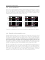
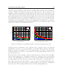
2.6.3
Discontinuous ILC
To use the ILC on the non-linear system the feedforward signal is calculated for all learning
filters (L). Depending on the reference position the appropriate feedforward is selected. This
results in a piecewise continuous signal, as can be seen in Figure 2.10. The feedforward signal
is filtered with the Q filter again with zero-phase filtering, to remove the non-smooth steps in
the signal.
0.2
All feedforward
Stepped feedforward
0.15
Input plant (u)
0.1
0.05
0
−0.05
−0.1
−0.15
0
0.2
0.4
0.6
0.8
1
Time [s]
Figure 2.10: Piecewise continuous feedforward signal.
2.6.4
Results
The results for the different motion profiles are described here. For the sinusoidal reference
both controllers converge to a steady state error, as can be seen in Figure 2.11. The PID-
2.6 Iterative learning control
15
controller converges within 15 trails, but the non-affine SMC controller needs 100 trails to
converge. Finally both controllers converge to the same rms-error. The exceptions are the
amplitude of 450 µm and higher, with the PID-controller. This is due the fact that the error
of the beam increases as the reference approaches the outer most position of the beam. At this
point a bump stop is attached which is hit, from which an even larger error is a result. In Figure
E.1 in Appendix E on page 33 all tracked amplitudes can be seen. For both controllers the
feedforward is injected before the plant, so in theory the repetitive error is reduced before the
remaining error goes through the controller. An explanation for the difference in convergence
speed between both controllers can be the fact that the Process Sensitivity (Sp ) for both
controllers is estimated in a slightly different way.
−6
5
−6
x 10
5
50 µm
250 µm
450 µm
4
4
3.5
3.5
3
2.5
2
1.5
3
2.5
2
1.5
1
1
0.5
0.5
0
50 µm
250 µm
450 µm
4.5
RMS−error
RMS−error
4.5
x 10
2
4
6
8
Trial (k)
10
(a) PID-controller.
12
14
0
10
20
30
40
50
Trial (k)
60
70
80
90
(b) Non-affine SMC controller.
Figure 2.11: RMS-error, depending on number of trials for sinusoidal trajectory.
In Figure 2.12, the performance of the controller can be compared for the case with and
without ILC. As can be seen, the performance of the PID-controller improves drastically,
within 15 iterations. For Figure 2.12 (b), the improvement is also visible, only this system
needs 100 iterations to converge to a steady state error. Both systems finally converge to the
same steady state error.
For the staircase reference with ∆r = 100 µm, both systems also converge to the same RMSvalue as for the sinusoidal case. The number of trials before convergence is for both controllers
the same. The initial RMS-error is much closer to the converged RMS-value, this explains the
fact that within 25 trial the system are converged. The results can be seen in Figure 2.13.
The results of the staircase profile with ∆r = 5 µm are depicted in Appendix E in Figure E.2.
As shown in Section 2.6.2, the repetitive and non-repetitive error can not be extinguished
from each other. This is why the ILC has no effect on the resulting RMS-error.
2.6 Iterative learning control
16
−5
4.5
−5
x 10
2.5
x 10
No ILC
ILC (k = 15)
ILC (k = 35)
No ILC
ILC (k = 15)
4
2
3.5
RMS−error
RMS−error
3
2.5
2
1.5
1
1.5
1
0.5
0.5
0
0
100
200
300
Amplitude [µm]
400
0
500
0
100
(a) PID-controller.
200
300
Amplitude [µm]
400
500
(b) Non-affine SMC controller.
Figure 2.12: Final RMS-error, depending on amplitude for sinusoidal trajectory.
−6
6
−6
x 10
1.5
5
Step: 1300 − 1200 [µm]
Step: 1100 − 1000 [µm]
Step: 900 − 800 [µm]
1
RMS−error [m]
4
RMS−error [m]
x 10
Step: 1300 − 1200 [µm]
Step: 1100 − 1000 [µm]
Step: 900 − 800 [µm]
3
2
0.5
1
0
5
10
15
Trail (k)
(a) PID-controller.
20
25
0
5
10
15
20
Trail (k)
(b) Non-affine SMC controller.
Figure 2.13: RMS-error, depending on number of trials for staircase trajectory.
25
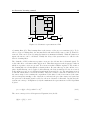
Chapter 3
Six Degrees of Freedom
As stated previously, the final goal of this project is to be able to actuate a levitating stage
with six degrees of freedom with a large range and high precision. A 6-DOF setup is designed
and fabricated. A schematic overview of the setup can be seen in Figure 3.1. In this setup six
permanent magnet sets and electromagnetic coils are used to actuate all degrees of freedom.
Also in this setup the repulsive magnets force is used to reduce the levitation current and to
avoid actuator saturation.
Horizontal actuators
Moving part
Base part
Permanent magnets
Capacitance sensors
Vertical actuators
Figure 3.1: 6-DOF setup.
The design and control of this Multi Input Multi Output system is described by D. Li in [14].
The position and orientation of the moving part with respect to the fixed world can be directly
estimated by using closed-form forward kinematics.
17
3.1 Iterative learning control
3.1
18
Iterative learning control
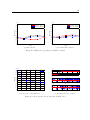
To see if Iterative Learning control can improve the performance of the 6-DOF system, simulations are done with several reference profiles. A schematic overview of the used Simulink
scheme can be seen in Figure D.2 on page 31. The used scheme is a simplification of the
system. The non-linear relation between the needed magnet force and the coil current is not
included in the system. But assuming this relation can be linearized as in the 1-DOF case
the results should still be valid. For the non-linear non-affine case [15] and [16] proof global
convergence for MIMO systems.
−5
−5
x
x 10
1.2
x 10
x
y
z
10
5
1
0
0
0.2
0.4
−6
0.8
1
0
−2
0
0.2
0.4
−6
2
0.8
RMS−error
2
0.6
y
x 10
0.6
0.8
1
0.6
0.4
psi
x 10
0.2
0
−2
0
0.2
0.4
0.6
Time [s]
0.8
(a) Resulting error step response.
1
0
1
2
3
4
5
6
Trail (k)
7
8
9
10
(b) Convergence of the error for spiral reference.
Figure 3.2: Results of ILC for a 6-DOF simulation.
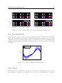
Three types of cases are simulated: a step in one direction, a step in three directions and a
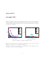
spiral reference. Most of the figures are included in Appendix E, on page 33. In Figure 3.2 (a),
the response of a step in the x-direction is shown. As can be seen, the cross talk to the other
directions is eliminated with ILC. In Figure E.3, the convergence of the error can be seen.
The error signal has a slightly higher peek-to-peek value and a higher frequency. In Figure 3.2
(b), the convergence of the error is shown for a spiral reference as can be seen in Figure E.5.
Figure E.4 shows the errors and convergence of the step response in three directions. As can
be seen all cases, the error of the actuated direction converges to a lower steady state value.
Chapter 4
Conclusion and Recommendations
4.1
Conclusion
The goal of this project was to improve the performance of a long range, sub-micrometer
reluctance actuator. And to implement a new real-time high performance data acquisition
and control system from Speedgoat. With the new hard- and software platform the design
and implementation times are reduced drastically with respect to the previous used Digital
Signal Processor (DSP). The installation of the real-time target took a lot more time than
expected and unexpected problems caused even more delays.
The previous designed controllers were successfully transferred to the real-time target and
similar responses were measured. The addition of Iterative Learning Control improved the
system performance for different reference profiles. For the small range reference profiles no
repetitive error was present, so ILC could not improve the results for these type of reference
profiles. An adapted ILC update scheme is used for the non-linear non-affine plant. The
feedforward signal is calculated using multiple learning filters and the appropriate one is
selected according to the reference position. This approach proofed to be suitable for this
problem. The use of ILC is also possible for the MIMO-case.
4.2
Recommendations
• To make a better estimate of the system parameters an other thin beam load sensor
should be used. With the used strain gauge only 25% of the range is used. Using the
full range will reduce the relative influence of noise.
• In the 1-DOF frequency response, two dominant resonances are present. These are
caused by the internal rods in the beam, used to attach the beam to the hinge. By
constraining the rods the resonances can be removed.
• The bump stops in the 1-DOF setup are hit when large amplitude reference signals are
used and the error increases at the end of the working range, causing the beam to hit the
bump stop. This introduces highly non-linear effects and influences the measurements.
19
4.2 Recommendations
20
• Redesign the robustness filter Q, depending on the used reference signal.
• In the current construction of the 6-DOF setup, permanent magnets are used in the
horizontal plane. In this plane no gravity compensation is needed.
• Estimate the time you think you need for the hardware implementation, multiply this
with 2.5 and add one week ;)
References
[1] L.J.P. Fevre, Design and construction of a 6 DOF positioning system with nanometer
accuracy, M.Sc. Thesis, Florida Institute of Technology (Dec. 2003).
[2] E.E. Visser, Modelling, instrumentation and control of a 6DOF positioning stage, M.Sc.
Thesis, Eindhoven University of Technology, Mechanical Engineering, DCT2004.112
(Nov. 2004).
[3] J. Simons, N.D. de Kleijn, Six degree of freedom stage with electromagnetic actuators,
Report international internship, Florida Institute of Technology (Apr. 2005)
[4] D. Li, Modeling and control of a high precision 6-DOF maglev positioning stage with
large range of travel, Dissertation for the degree of Doctor of philosophy in mechanical
engineering, Florida Institute of Technology (Dec. 2008)
[5] J.J. Bolder, J. de Boeij, H.M. Gutiérrez, M. Steinbuch Non-affine sliding mode control of
a reluctance actuator with passive gravity compensation, Florida Institute of Technology,
Unpublished
[6] D. Li, H.M. Gutierrez, Precise motion control of a hybrid magnetic suspension actuator
with large travel, Industrial Electronics (Nov. 2008)
[7] H.K. Khalil, Nonlinear Systems, 3rd. edition. Prentice Hall (Dec. 2001)
[8] J.J. Slotine, W. Li, Applied Nonlinear Control, Prentice-Hall (1991)
[9] H.M. Gutierrez, P.I. Ro, Magnetic servo levitation by sliding-mode control of nonaffine
systems with algebraic input invertibility, IEEE Transactions on Industrial Electronics,
vol. 52, no. 5 (Oct. 2005)
[10] J.X. Xu, S.K. Panda, T.H. Lee, Real-time Iterative Learning Control - Design and Applications, National University of Singapore (2009)
[11] K.L. Moore, Iterative learning control for deterministic systems, Springer, Berlin (1993)
[12] T. Donkers, Robust Iterative Learning Control - A Literature Survey, Eindhoven University of Technology, DCT 2007-21 (Feb. 2007)
[13] M. Steinbuch, M.J.G. Molengraft, Iterative Learning Control of Industrial Motion Systems, Eindhoven University of Technology (2000)
21
REFERENCES
22
[14] D. Li, H.M. Gutiérrez, Observer-based Sliding Mode Control of a 6-DOF Precision Maglev
Positioning Stage, Florida Institute of Technology (Nov. 2008)
[15] J.X. Xu, Y. Tan, New Iterative Learning Control approaches for Nonlinear Non-affine
MIMO Dynamic Systems, National University of Singapore (Jun. 2001)
[16] J. Kang, A New Iterative Learning Control Scheme with Global Convergece for MIMO
Nonlinear Dynamic Systems, Tianjij University (May 2010)
Appendix A
Nomenclature
g
F
u
x
x1
x2
x̂
m
k1
k2
k3
g0
c
u0
Fm
P
S
Sp
L
Q
Gap
Force
Input to coil
Plant states
Position state
Velocity state
Estimated states
Mass
Parameter
Parameter
Parameter
Initial gap
Damping
Virtual input
Measured force
Plant
Sensitivity
Process Sens.
Learning filter
Robustness filter
[µm]
[N ]
[A]
[−]
[m]
[m/s]
[−]
[kg]
[−]
[−]
[−]
[µm]
[N s/m]
[0 N/kg 0 ]
[N ]
[−]
[−]
[−]
[−]
[−]
Gap between beam and sensor
Netto force on beam
Current through the coil
States of the plant
Position state of the plant
Velocity state of the plant
Estimated plant states
Virtual mass of the beam
Parameter related to the permanent magnet force
Parameter related to the permanent magnet force
Parameter related to the elektro magnetic force
Initial gap between beam and sensor
Damping of the beam
Virtual input, force on a unit mass
Netto measured force on load cell
Transfer function of the plant
Transfer function of the Sensitivity
Transfer function of the Process Sensitivity
Transfer function of the Learning filter
Transfer function of Robustness filter
23
Appendix B
Installing the Speedgoat
The used hardware platform is the performance real-time target machine from Speedgoat.
The data in and outputs of the system can be integrated in a simulink model. When running
the real-time application, the xPC toolbox from matlab compiles an executable which runs
real-time on the target. This way high sampling frequencies up to 40 kHz (depending on the
used hardware) can be reached. The target is connected via a standard LAN-connection to
a host computer, running matlab and the compiler. During the experiment no adjustments
can be made to the simulink block scheme, only pre defined variables can be adjusted. The
data collected during the experiment is stored in the 4 GB RAM. Storing data on the internal
hard drive is also possible, but this is not used during these experiments. In Figure B.1 the
real-time target in the test setup is shown.
Figure B.1: Real-time target in the setup.
B.1
IO-cards
The used IO-cards determine the resolution of the measurements. The analog input/output
card has a resolution of 16-bit, with 8 differential inputs and 8 output channels. The input
24
B.2 Installation
25
and output range is +/- 10 volts. One output is used as an input to the current amplifier.
The inputs are used for the position measurement, the load cell output, the supply voltage to
the load cell and a current clamp to measure the actual current through the coil. The digital
input card supports 32 channels, grouped in clusters of 8 with common grounds. The inputs
are used for an emergency switch and to check if the power supply is on.
B.2
Installation
The installation of the real-time machine is described in the user manual. In this section
the installation of the target is described as executed during this internship. Also some hints
and tips are given. This installation guide is from personal experience, this means that no
guarantees can be given and that you still should be careful (especially when using different
software versions or hardware).
1. Install matlab r2009b or the one with the service pack (r2009bSP1) 32-bit version, even
if your host computer is a 64-bit system (the xPC toolbox version v4.2 only works with
32-bit matlab).
2. Make sure that the following toolboxes are installed:
• Simulink
• Real-time workshop
• xPC Target (v4.2)
3. Close matlab (if it is not already closed)
4. Install a compiler (Microsoft Visual Studio). The free express-version will work. The
installation file is in the Software folder (vcsetup.exe)
5. Install speedgoat software. The installation file is in the software folder ...\Xpc Speedgoat
CD\speedgoat_R2009b
6. Start Matlab
7. Rehash the toolboxes: » rehash toolbox
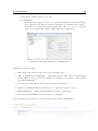
8. Open the xPC Target Explorer: » xpcexplr
• Compilers(s) Configuration
- Select C compiler: Visual C
- Compiler path (in this case): C:\Program Files (x86)\Microsoft Visual
Studio 9.0
• Set communication. For host target communication see Figure B.2.
• DLM’s: The DLM node represents the current working directory. This directory
contains all instances of a build xPC Target application
• Settings: Target RAM size (MB): Auto
B.2 Installation
26
• Appearance: Enable target scope: Yes
• Configuration:
- Booting with a floppy: Create a boot disk. Startup the target with floppy
drive attached. New files are loaded to the target pc. Restart after loading.
- Network boot: Insert MAC address target (00 − 1B − 21 − 31 − 79 − 12) and
click create Network Boot Image (this setting is recommended!)
Figure B.2: xPC Target Explorer, communication.
Starting the real-time target:
1. Turn on the blue switch on the back of the real-time target
2. Run: » xpcnetboot(’TargetPC1’). This starts up the xPC Target Network Boot
Server, which is used to load the network boot image to the target pc and upload
the build Simulink files.
3. Pres the blue round button on the front of the xPC to start up.
4. Option: » xpctargetping, to assure there is a connection (answer: success)
5. Build Simulink file, compile it with Ctrl+B and start: » start(tg)
6. Stop the file from running (before end time): » stop(tg)
The following m-code was used to start the target and build the simulink files.
%% Starting up of the xPC
% Check with a dialog if the xPC is on.
choice = questdlg('Is the xPC on?','Dialog','Yes','No','Yes');
if strcmp(choice,'No')
questdlg('Turn on the main power switch on the xPC. And pres OK.','Dialog','Ok','Ok');
disp('wait')
% Acknowledge a key is pressed
B.3 Tips and tricks
pause(5)
xpcnetboot('TargetPC1')
27
% Wait for the network card to start
% Start up the xPC network boot server
questdlg('Turn on the xPC (blue round button). And pres Ok.','Dialog','Ok','Ok');
while ¬strcmpi(xpctargetping,'success')
pause(1)
fprintf('.')
end
disp(' xPC started up')
% Wait until the xPc has started up
end
%% Build / compile the model and upload to the xPC
% Check with a dialog if the model has to be build and uploaded
choice = questdlg('Build and upload the model?','Dialog','Yes','No','Yes');
if strcmp(choice,'Yes')
open_system('simulink_file_name');
% Open the model
set_param('simulink_file_name','RTWVerbose','off');
% Configure RTW for a non−Verbose build
rtwbuild('simulink_file_name');
% Build and download to the target
close_system('simulink_file_name',0);
% Close the model
tg = xpc;
% Create an xPC Target Object
end
B.3
Tips and tricks
• Watch out for data wrapping. If there are more samples acquired than possible, the
first samples are over written. Check for data wrapping with: » tg.NumLogWraps. The
answer gives the number of times the data is over written.
• To be able to obtain high sampling frequencies, the communication between the host
and the target should be minimized. When using a m-file to compile, run and process
the data, the following construction can be used to minimize communication and wait
with retrieving the data:
set(tg,'StopTime',stop_time)
start(tg);
% Set the simulation time
% Start running the model
pause(stop_time+0.5)
% Don't communicate with xPc during run
while ¬strcmpi(tg.Status,'stopped')
pause(0.2)
sprintf('Communicate xPC \n')
end
% Is the run complete?
• Data can be retrieved in two ways. With an outport in Simulink or with a host
scope. The data from an outport can be accessed with: » t = tg.TimeLog and » y
= tg.OutputLog. The data from a host scope can be retrieved with the following script:
B.3 Tips and tricks
28
% Get a handle to host scopes
scope_name = getscope(tg,1);
% Retreive data
t
= scope_name.time;
y
= scope_name.Data(:,1);
Wacht out: The time stamps of the host scopes can be different than tg.time!
• The Task Execution Time (TET) is the time the real-time target needs to calculate
the next output values. To increase the sample frequency check: » tg.TETLog for the
execution time.
• Variables can be changed between tests without building and uploading the complete
Simulink file. First get the parameter ID. The name is build up from the sub block names
the parameter is contained and the name of the parameter is self, divided with a slash:
» param_id = getparamid(tg,’sub_block/param_name’,’Value’). The variable can
be set with: » setparam(tg,param_id,0).
• Do not change any setting in the BIOS. The settings in the BIOS disable some
processes which can cause interrupts on the CPU. When an interrupt occurs during
a simulation, the Task Execution Time (TET) goes up drastically. When the TET is
higher than the set sampling time, the simulation is stopped.
Appendix C
Load cell calibration
The used load cell to do the parameter estimation is a Thin Beam Sensor for up to 10 pounds
(TBS-10). The sensor is manufactured by Transducer Techniques. More specifications about
the load cell can be found at: www.ttloadcells.com/TBS-Load-Cell.cfm. Before doing any
measurements it is wise to recalibrate the load cell for both compressive and tensile loads.
The load cell is rated to be powered with 10 volts, but it can be safely overloaded up to 150
%. Using 15 volts increases the resolution of the measurements. The tensile force can be
applied by clamping the beam to one bump stop and attaching a string to the other side of
the sensor. With pulley’s the string is directed vertically. Weights can be attached to the
string for calibration. For compression loads the sensor is attached to the lead screw and
pulled against the support. First attach the sensor to the the inner bolt and turn the outer
bolt until the sensor is clamped against the support. In Figure C.1 the setup is shown.
(a) Compression.
(b) Tension.
Figure C.1: Setup for calibrating the load cell.
The output voltage of the load cell is linear with the supply voltage. To check the supply
voltage from different measurements the voltage is logged with the xPC. Because the input
range of the analog data acquisition card is limited to +/- 10 volt, a voltage divider is used
to reduce the voltage to the working range of the analog card.
29
30
After the calibration is done, 10 % is added to the measured force. This is due to the offset
of the force sensor with respect to the coil.
Figure C.2: Drawer with load cells and mounting brackets.
In the lab there is a drawer with a box in it with other types of load cells and load cell
mounting brackets. In this drawer you can also find some loose capacitive sensors and the
calibration reports of the capacitive sensors. The drawer has no label, but is right from the
’mounting hardware’ drawer, as can be seen in Figure C.2.
Appendix D
Simulink schemes
g_ref_ddot
g_ref_ddot
ILC_ff
g_ref_dot
e_dot
g_ref_dot
g_ref
u
in
Saturation
Amp.
e
g_ref
out
Sensitivity
in
in
out
Input
PMC-16AIO 1
g_hat_dot
Reference
g
Kill
g
g_hat
u
g_hat_dot
Non. lin. obs.
g_hat
Non-affine SMC
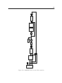
Figure D.1: Simulink scheme for the non-affine SMC-controller.
ref_ddot
ref_acc
ILC_ff
f_tau
vel_est
e_dot
ref_vel
f_tau
e
ref_pos
in
out
f_tau
pos
pos
pos_dist
Sensor dist.
Sensi.
Plant
Ref
pos
SMC-controller
pos
vel_c
vel_est
Velocity Conv.
Figure D.2: Simulink scheme for the 6-DOF system.
31
pos_dist
High Gain Observer
Reference
g_ref
g_ref_dot
g_ref_ddot
e
u_prime
PD controller
e_dot
u_prime
I_squared
feedback_linearization
g_hat
Saturation
Amp.
sqrt(u)
out
Sensitivity
in
ILC_ff
in
Kill
out
PMC-16AIO 1
in
Input
g
u
g
g_hat
Non. lin. obs.
g_hat_dot
32
Figure D.3: Simulink scheme for the PID-controller.
Appendix E
Graphs ILC
Figure E.1: Convergence plot of both controllers for 15 trails. As can be seen, the performance
for large amplitudes is deviating from other RMS-error values. This is due the fact that the
beam hits a physical bump stop when the error is increasing. From this physical contact the
error increases even further.
−5
−5
x 10
3.5
0 µm
50 µm
100 µm
150 µm
200 µm
250 µm
300 µm
350 µm
400 µm
450 µm
480 µm
485 µm
3
RMS−error
2.5
2
1.5
2
1.5
1
0.5
0.5
2
4
6
8
Trial (k)
10
12
0 µm
50 µm
100 µm
150 µm
200 µm
250 µm
300 µm
350 µm
400 µm
450 µm
500 µm
2.5
1
0
x 10
3
RMS−error
3.5
0
14
(a) PID-controller.
2
4
6
8
Trial (k)
10
12
14
(b) Non-affine SMC controller.
Figure E.1: RMS-error, depending on number of trials.
Figure E.2: Convergence plot for the staircase profile with ∆r = 5µm. As can be seen the
RMS-error does not decrease as explained in Section 2.6.4.
In Figure E.3, E.4 and E.5, the convergence of the RMS-error and the resulting error after
convergence is shown for the 6-DOF simulation.
33
34
−6
1
−6
x 10
1
Step: 1300 − 1200 [µm]
Step: 1100 − 1000 [µm]
Step: 900 − 800 [µm]
0.8
0.8
0.7
0.7
0.6
0.5
0.4
0.6
0.5
0.4
0.3
0.3
0.2
0.2
0.1
0.1
0
1
1.5
2
2.5
3
Trail (k)
3.5
4
4.5
Step: 1300 − 1200 [µm]
Step: 1100 − 1000 [µm]
Step: 900 − 800 [µm]
0.9
RMS−error [m]
RMS−error [m]
0.9
x 10
5
0
1
1.5
(a) PID-controller.
2
2.5
3
Trail (k)
3.5
4
4.5
5
(b) Non-affine SMC controller.
Figure E.2: RMS-error, depending on number of trials.
−5
1
x 10
−5
x
x 10
x
10
0.9
5
0.8
0
0
0.7
0.2
0.4
RMS−error
−6
0.6
2
0.5
0
0.4
−2
0.3
0.2
0.8
1
0.2
0.6
0.8
1
0.6
Time [s]
0.8
1
0.4
psi
x 10
0
0.1
0
0
−6
2
0.6
y
x 10
1
2
3
4
Trail (k)
5
6
(a) Convergence of the RMS-error.
7
−2
0
0.2
0.4
(b) Resulting error and crosstalk.
Figure E.3: Step response in one direction (6-DOF case).
35
−5
−5
x 10
x
y
ψ
1.8
1.6
−5
x
x 10
x 10
−5
y
4
4
4
2
2
2
0
0
0
−2
−2
−2
−4
−4
x 10
z
0.2
0.4
RMS−error
1.4
0.2
0.4
0.6
−4
0.2
0.4
0.6
0.6
1.2
−5
x 10
1
0.8
−5
phi
x 10
−5
the
x 10
4
4
4
2
2
2
0
0
0
−2
−2
−2
psi
0.6
−4
1
2
3
4
5
6
Trail (k)
7
8
9
10
−4
0.2
0.4
0.6
(a) Convergence of the RMS-error.
−4
0.2
0.4
0.6
0.2
0.4
0.6
(b) Resulting error.
Figure E.4: Step response in three directions (6-DOF case).
−5
1.2
x 10
x
y
z
1
−4
x 10
Reference
Position
3.5
3
2.5
z [m]
RMS−error
0.8
0.6
2
1.5
1
0.4
1
0.2
1
0
−4
x 10
0
1
2
3
4
5
6
Trail (k)
7
8
(a) Convergence of the RMS-error.
9
10
y [m]
0
−1
−1
x [m]
(b) Reference position and position.
Figure E.5: Spiral reference (6-DOF case).
−4
x 10