Download Chapter 7

7
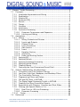
Chapter 7 Audio Processing .............................................................. 2
7.1 Concepts .................................................................................. 2
7.1.1 Amplitude Adjustments and Mixing ........................................ 2
7.1.2 Equalization ........................................................................ 2
7.1.3 Graphic EQ.......................................................................... 3
7.1.4 Parametric EQ ..................................................................... 4
7.1.5 Reverb ............................................................................... 7
7.1.6 Flange .............................................................................. 10
7.1.7 Vocoders .......................................................................... 11
7.1.8 Autotuners ........................................................................ 12
7.1.9 Dynamics Processing .......................................................... 13
7.1.9.1 Dynamics Compression and Expansion ............................ 13
7.1.9.2 Limiting and Gating ...................................................... 18
7.2 Applications ............................................................................ 20
7.2.1 Mixing .............................................................................. 20
7.2.1.1 Mixing Contexts and Devices ......................................... 20
7.2.1.2 Inputs and Outputs ...................................................... 23
7.2.1.3 Channel Strips ............................................................. 23
7.2.1.4 Input Connectors ......................................................... 25
7.2.1.5 Gain Section ................................................................ 25
7.2.1.6 Insert ......................................................................... 28
7.2.1.7 Equalizer Section .......................................................... 29
7.2.1.8 Auxiliaries ................................................................... 31
7.2.1.9 Fader and Routing Section ............................................. 33
7.2.2 Applying EQ ...................................................................... 37
7.2.3 Applying Reverb ................................................................ 39
7.2.4 Applying Dynamics Processing ............................................. 42
7.2.5 Applying Special Effects ...................................................... 43
7.2.6 Creating Stereo ................................................................. 44
7.2.7 Capturing the Four-Dimensional Sound Field ......................... 44
7.3 Science, Mathematics, and Algorithms ....................................... 54
7.3.1 Convolution and Time Domain Filtering ................................. 54
7.3.2 Low-Pass, High-Pass, Bandpass, and Bandstop Filters ............ 57
7.3.3 The Convolution Theorem ................................................... 59
7.3.4 Diagramming Filters and Delays .......................................... 61
7.3.5 FIR and IIR Filters in MATLAB .............................................. 61
7.3.6 The Digital Signal Processing Toolkit in MATLAB ..................... 63
7.3.7 Creating Your Own Convolution Reverb ................................. 63
7.3.8 Experiments with Filtering: Vocoders and Pitch Glides ........... 66
7.3.9 Filtering and Special Effects in C++ ...................................... 68
7.3.9.1 Real-Time vs. Off-Line Processing ................................... 68
7.3.9.2 Dynamics Processing .................................................... 68
7.3.10
Flange ........................................................................... 68
7.4 References ............................................................................. 68
This material is based on work supported by the National Science Foundation under CCLI Grant DUE 0717743,
Jennifer Burg PI, Jason Romney, Co-PI.
Digital Sound & Music: Concepts, Applications, & Science, Chapter 7, last updated 7/29/2013
7 Chapter 7 Audio Processing
7.1 Concepts
7.1.1
Amplitude Adjustments and Mixing
We've entitled this chapter "Audio Processing" as if this is a separate, discrete topic within the
realm of sound. But, actually, everything we do to audio is a form of processing. Every tool,
plug-in, software application, and piece of gear is essentially an audio processor of some sort.
What we set out to do in this chapter is to focus on particular kinds of audio processing, covering
the basic concepts, applications, and underlying mathematics of these.
One of the most straightforward types of audio processing is amplitude adjustment –
something as simple as turning up or down a volume control. In the analog world, a change of
volume is achieved by changing the voltage of the audio signal. In the digital world, it's
achieved by adding to or subtracting from the sample values in the audio stream – just simple
arithmetic.
The mixing of two digital audio signals is another simple example of audio processing.
Digital mixing is accomplished by adding sample values together – again, just arithmetic. But
even though volume changes and mixing involve simple mathematical operations, they are
among the most important processes we apply to audio because they potentially are very
destructive. Add too much to a signal and you have clipping – seriously distorted audio.
Subtract too much, and you have silence. No application of filters or fancy digital signal
processing can fix clipping or complete loss of signal.
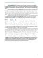
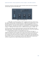
An important form of amplitude processing is normalization, which entails increasing
the amplitude of the entire signal by a uniform proportion. Normalizers achieve this by allowing
you to specify the maximum level you want for the signal, in percentages or dB, and increasing
all of the samples’ amplitudes by an identical proportion such that the loudest existing sample is
adjusted up or down to the desired level. This is helpful in maximizing the use of available bits
in your audio signal, as well as matching amplitude levels across different sounds. Keep in mind
that this will increase the level of everything in your audio signal, including the noise floor.
Figure 7.1 Normalizer from Adobe Audition
7.1.2
Equalization
The previous section dealt with amplitude processing. We now turn to processing that affects
frequencies.
2
Digital Sound & Music: Concepts, Applications, & Science, Chapter 7, last updated 7/29/2013
Audio equalization, more commonly referred to as EQ, is the process of altering the
frequency response of an audio signal. The purpose of equalization is to increase or decrease the
amplitude of chosen frequency components in the signal. This is achieved by applying an audio
filter.
EQ can be applied in a variety of situations and for a variety of reasons. Sometimes, the
frequencies of the original audio signal may have been affected by the physical response of the
microphones or loudspeakers, and the audio engineer wishes to adjust for these factors. Other
times, the listener or audio engineer might want to boost the low end for a certain effect, "even
out" the frequencies of the instruments, adjust frequencies of a particular instrument to change its
timbre, to name just a few of the many possible reasons for applying EQ.
Equalization can be achieved by either hardware or software. Two commonly-used types
of equalization tools are graphic and parametric EQs. Within these EQ devices, low-pass,
high-pass, bandpass, bandstop, low shelf, high shelf, and peak-notch filters can be applied.
7.1.3
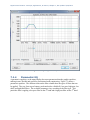
Graphic EQ
A graphic equalizer is one of the most basic types of EQ. It consists of a number of fixed,
individual frequency bands spread out across the audible spectrum, whose amplitudes can simply
be turned up or down. To match our non-linear perception of sound, the center frequencies of
the bands are spaced logarithmically. A graphic EQ is shown in Figure 7.2. This equalizer has
31 frequency bands, with center frequencies at 20 Hz, 25, Hz, 31 Hz, 40 Hz, 50 Hz, 63 Hz, 80
Hz, and so forth in a logarithmic progression up to 20 kHz. Each of these bands can be raised or
lowered in amplitude individually to achieve an overall EQ shape.
While graphic equalizers are fairly simple to understand, they are not very efficient to use
since they often require that you manipulate several controls to accomplish a single EQ effect. In
an analog graphic EQ, each slider represents a separate filter circuit that also introduces noise
and manipulates phase independently of the other filters. These problems have given graphic
equalizers a reputation for being noisy and rather messy in their phase response. The interface for
a graphic EQ can also be misleading because it gives the impression that you're being more
precise in your frequency processing than you actually are. That single slider for 1000 Hz can
affect anywhere from one third of an octave to a full octave of frequencies around the center
frequency itself, and consequently each actual filter overlaps neighboring ones in the range of
frequencies it affects. In the digital world, a graphic EQ can be designed to avoid some of these
problems by having the graphical sliders simply act as a user interface, when in fact the slider
settings are used by the DSP to build a single coherent filter. Even with this enhancement,
graphic EQs are generally not preferred by experiences professionals.
3
Digital Sound & Music: Concepts, Applications, & Science, Chapter 7, last updated 7/29/2013
Figure 7.2 Graphic EQ in Audacity
7.1.4
Parametric EQ
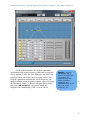
A parametric equalizer, as the name implies, has more parameters than the graphic equalizer,
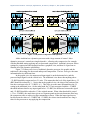
making it more flexible and useful for professional audio engineering. Figure 7.3 shows a
parametric equalizer. The different icons on the filter column show the types of filters that can
be applied. They are, from top to bottom, peak-notch (also called bell), low-pass, high-pass, low
shelf, and high shelf filters. The available parameters vary according to the filter type. This
particular filter is appling a low-pass filter on the 4th band and a high-pass filter on the 5th band.
4
Digital Sound & Music: Concepts, Applications, & Science, Chapter 7, last updated 7/29/2013
Figure 7.3 Parametric EQ in Cakewalk Sonar
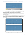
For the peak-notch filter, the frequency parameter
corresponds to the center frequency of the band to which the
filter is applied. For the low-pass, high-pass, low-shelf, and
high-shelf filters, which don’t have an actual “center,” the
frequency parameter represents the cut-off frequency. The
numbered circles on the frequency response curve correspond
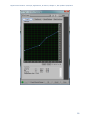
the filter bands. Figure 7.4 shows a low-pass filter in band 1
where the 6 dB downpoint – the point at which the
frequencies are attenuated by 6 dB – is set to 500 Hz.
 Aside: The term
"paragraphic EQ" is
used for a combination
of a graphic and
parametric EQ, with
sliders to change
amplitudes and
parameters that can be
set for Q, cutoff
frequency, etc.
to
5
Digital Sound & Music: Concepts, Applications, & Science, Chapter 7, last updated 7/29/2013
Figure 7.4 Low-pass filter in a parametric EQ with cut-off frequency of 500 Hz
The gain parameter is the amount by which the corresponding frequency band will be
boosted or attenuated. The gain cannot be set for low or high-pass filters, as these types of filters
are designed to eliminate all frequencies beyond or up to the cut-off frequency.
The Q parameter is a measure of the height vs. the width of the frequency response curve.
A higher Q value creates a steeper peak in the frequency response curve compared to a lower
one, as shown in Figure 7.5.
Some parametric equalizers use a bandwidth parameter instead of Q to control the range
of frequencies for a filter. Bandwidth works inversely from Q in that a larger value of bandwidth
represents a larger range of frequencies. The unit of measurement for bandwidth is typically an
octave. A bandwidth value of 1 represents a full octave of frequencies between the 6 dB down
points of the filter.
Q = 1.0
Q = 5.2
Figure 7.5 Comparison of Q values for two peak filters
6
Digital Sound & Music: Concepts, Applications, & Science, Chapter 7, last updated 7/29/2013
7.1.5
Reverb
When you work with sound either live or recorded, the sound is typically captured with the
microphone very close to the source of the sound. With the microphone very close, and
particularly in an acoustically treated studio with very little reflected sound, it is often desired or
even necessary to artificially add a reverberation effect to create a more natural sound, or perhaps
to give the sound a special effect. Typically a very dry initial recording is preferred, so that
artificial reverberation can be applied more uniformly and with greater control.
There are several methods for adding reverberation. Before the days of digital processing
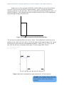
this was accomplished using a reverberation chamber. A reverberation chamber is simply a
highly reflective, isolated room with very low background noise. A loudspeaker is placed at one
end of the room and a microphone is placed at the other end. The sound is played into the
loudspeaker and captured back through the microphone with all the natural reverberation added
by the room. This signal is then mixed back into the source signal, making it sound more
reverberant. Reverberation chambers vary in size and construction, some larger than others, but
even the smallest ones would be too large for a home, much less a portable studio.
Because of the impracticality of reverberation chambers, most artificial reverberation is
added to audio signals using digital hardware processors or software plug-ins, commonly called
reverb processors. Software digital reverb processors use software algorithms to add an effect
that sounds like natural reverberation. These are essentially delay algorithms that create copies of
the audio signal that get spread out over time and with varying amplitudes and frequency
responses.
A sound that is fed into a reverb processor will come out of that processor with thousands
of copies or virtual reflections. As described in Chapter 4, there are three components of a
natural reverberant field. A digital reverberation algorithm attempts to mimic these three
components.
The first component of the reverberant field is the direct sound. This is the sound that
arrives at the listener directly from the sound source without reflecting from any surface. In
audio terms, this is known as the dry or unprocessed sound. The dry sound is simply the
original, unprocessed signal passed through the reverb processor. The opposite of the dry sound
is the wet or processed sound. Most reverb processors include a wet/dry mix that allows you to
balance the direct and reverberant sound. Removing all of the dry signal leaves you with a very
ambient effect, as if the actual sound source was not in the room at all.
The second component of the reverberant field is the early reflections. Early reflections
are sounds that arrive at the listener after reflecting from the first one or two surfaces. The
number of early reflections and their spacing vary as a function of the size and shape of the
room. The early reflections are the most important factor contributing to the perception of room
size. In a larger room, the early reflections take longer to hit a wall and travel to the listener. In a
reverberation processor, this parameter is controlled by a pre-delay variable. The longer the predelay, the longer time you have between the direct sound and the reflected sound, giving the
effect of a larger room. In addition to pre-delay, controls are sometimes available for determining
the number of early reflections, their spacing, and their amplitude. The spacing of the early
reflections indicates the location of the listener in the room. Early reflections that are spaced
tightly together give the effect of a listener who is closer to a side or corner of the room. The
amplitude of the early reflections suggests the distance from the wall. On the other hand, low
amplitude reflections indicate that the listener is far away from the walls of the room.
7
Digital Sound & Music: Concepts, Applications, & Science, Chapter 7, last updated 7/29/2013
The third component of the reverberant field is the reverberant sound. The reverberant
sound is made of up all the remaining reflections that have bounced around many surfaces before
arriving at the listener. These reflections are so numerous and close together that they are
perceived as a continuous sound. Each time the sound reflects off a surface, some of the energy
is absorbed. Consequently, the reflected sound is quieter than the sound that arrives at the surface
before being reflected. Eventually all the energy is absorbed by the surfaces and the
reverberation ceases. Reverberation time is the length of time it takes for the reverberant sound
to decay by 60 dB, effectively a level so quiet it ceases to be heard. This is sometimes referred to
as the RT60, or also the decay time. A longer decay time indicates a more reflective room.
Because most surfaces absorb high frequencies more efficiently than low frequencies, the
frequency response of natural reverberation is typically weighted toward the low frequencies. In
reverberation processors, there is usually a parameter for reverberation dampening. This applies
a high shelf filter to the reverberant sound that reduces the level of the high frequencies. This
dampening variable can suggest to the listener the type of reflective material on the surfaces of
the room.
Figure 7.6 shows a popular reverberation plug-in. The three sliders at the bottom right of
the window control the balance between the direct, early reflection, and reverberant sound. The
other controls adjust the setting for each of these three components of the reverberant field.
Figure 7.6 The TrueVerb reverberation plug-in from Waves
8
Digital Sound & Music: Concepts, Applications, & Science, Chapter 7, last updated 7/29/2013
The reverb processor pictured in Figure 7.7 is based on a complex computation of delays
and filters that achieve the effects requested by its control settings. Reverbs such as these are
often referred to as algorithmic reverbs, after their unique mathematical designs.
There is another type of reverb processor called a convolution reverb, which creates its
effect using an entirely different process. A convolution reverb processor uses an impulse
response (IR) captured from a real acoustic space, such as the
one shown in Figure 7.7. An impulse response is essentially
 Aside: Convolution is a
the recorded capture of a sudden burst of sound as it occurs in
mathematical process that
operates in the time-domain
a particular acoustical space. If you were to listen to the IR,
– which means that the
which in its raw form is simply an audio file, it would sound
input to the operation
like a short “pop” with somewhat of a unique timbre and
consists of the amplitudes of
decay tail. The impulse response is applied to an audio signal
the audio signal as they
change over time.
by a process known as convolution, which is where this
Convolution in the timereverb effect gets its name. Applying convolution reverb as a
domain has the same effect
filter is like passing the audio signal through a representation
as mathematical filtering in
of the original room itself. This makes the audio sound as if it
the frequency domain,
where the input consists of
were propagating in the same acoustical space as the one in
the magnitudes of frequency
which the impulse response was originally captured, adding
components over the
its reverberant characteristics.
frequency range of human
hearing. Filtering can be
With convolution reverb processors, you lose the extra
done in either the time
control provided by the traditional pre-delay, early reflections,
domain or the frequency
and RT60 parameters, but you often gain a much more natural
domain, as will be explained
reverberant effect. Convolution reverb processors are typically
in Section 3.
more CPU intensive than their more traditional counterparts,
but with the speed of modern CPU’s, this is not a big concern.
Figure 7.7 shows an example of a convolution reverb plug-in.
9
Digital Sound & Music: Concepts, Applications, & Science, Chapter 7, last updated 7/29/2013
Figure 7.7 A convolution reverb processor from Logic
7.1.6
Flange
Flange is the effect of combing out frequencies in a continuously changing frequency range.
The flange effect is created by adding two identical audio signals, with one slightly delayed
relative to the other, usually on the order of milliseconds or samples. The effect involves
continuous changes in the amount of delay, causing the combed frequencies to sweep back and
forth through the audible spectrum.
In the days of analog equipment like tape decks, flange was created mechanically in the
following manner: Two identical copies of an audio signal (usually music) were played,
simultaneously and initially in sync, on two separate tape decks. A finger was pressed slightly
against the edge (called the flange) of one of the tapes, slowing down its rpms. This delay in one
of the copies of the identical waveforms being summed resulted in the combing out of a
corresponding fundamental frequency and its harmonics. If the pressure increased continuously,
the combed frequencies swept continuously through some range. When the finger was removed,
the slowed tape would still be playing behind the other. However, pressing a finger against the
other tape could sweep backward through the same range of combed frequencies and finally put
the two tapes in sync again.
Artificial flange can be created through mathematical manipulation of the digital audio
signal, as shown in the exercise associated with Section 7.3.10. However, to get a classic
sounding flanger, you need to do more than simply delay a copy of the audio. This is because
tape decks used in analog flanging had inherent variability that caused additional phase shifts and
frequency combing, and thus they created a more complex sound. This fact hasn’t stopped clever
10
Digital Sound & Music: Concepts, Applications, & Science, Chapter 7, last updated 7/29/2013
software developers, however. The flange processor shown in Figure 7.8 from Waves is one that
includes a tape emulation mode and includes presets that emulate several kinds of vintage tape
decks and other analog equipment.
Figure 7.8 A digital flange processor
7.1.7
Vocoders
A vocoder (voice encoder) is a device that was originally developed for low bandwidth
transmission of voice messages, but is now used for special voice effects in music production.
The original idea behind the vocoder was to encode the essence of the human voice by
extracting just the most basic elements – the consonant sounds made by the vocal chords and the
vowel sounds made by the modulating effect of the mouth. The consonants serve as the carrier
signal and the vowels (also called formants) serve as the modulator signal. By focusing on the
most important elements of speech necessary for understanding, the vocoder encoded speech
efficiently, yielding a low bandwidth for transmission. The resulting voice heard at the other end
of the transmission didn't have the complex frequency components of a real human voice, but
enough information was there for the words to be intelligible.
Today’s vocoders, used in popular music, combine voice and instruments to make the
instrument sound as if it’s speaking, or conversely, to make a voice have a robotic or “techno”
sound. The concept is still the same, however. Harmonically-rich instrumental music serves as
the carrier, and a singer’s voice serves as the modulator. An example of a software vocoder plugin is shown in Figure 7.9.
11
Digital Sound & Music: Concepts, Applications, & Science, Chapter 7, last updated 7/29/2013
Figure 7.9 A vocoder processor
7.1.8
Autotuners
An autotuner is a software or hardware processor that is able to move a pitch of the human
voice to the frequency of the nearest desired semitone. The original idea was that if the singer
was slightly off-pitch, the autotuner could correct the pitch. For example, if the singer was
supposed to be on the note A at a frequency of 440 Hz, and she was actually singing the note at
435 Hz, the autotuner would detect the discrepancy and
make the correction.
 Aside: Autotuners have also
If you think about how an autotuner might be
been used in popular music as an
effect rather than a pitch correction.
implemented, you'll realize the complexities involved.
Snapping a pitch to set semitones
Suppose you record a singer singing just the note A,
can create a robotic or artificial
which she holds for a few seconds. Even if she does
sound that adds a new complexion
this nearly perfectly, her voice contains not just the
to a song. Cher used this effect in
her 1998 Believe album. In the
note A but harmonic overtones that are positive integer
2000s, T-Pain further popularized
multiples of the fundamental frequency. Your
its use in R&B and rap music.
algorithm for the software autotuner first must detect
the fundamental frequency – call it f – from among all
the harmonics in the singer's voice. It then must determine the actual semitone nearest to f.
Finally, it has to move f and all of its harmonics by the appropriate adjustment. All of this
sounds possible when a single clear note is steady and sustained long enough for your algorithm
to analyze it. But what if your algorithm has to deal with a constantly-changing audio signal,
which is the nature of music? Also, consider the dynamic pitch modulation inherent in a singer’s
vibrato, a commonly used vocal technique. Detecting individual notes, separating them one from
the next, and snapping each sung note and all its harmonics to appropriate semitones is no trivial
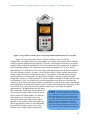
task. An example of an autotune processor is shown in Figure 7.10.
12
Digital Sound & Music: Concepts, Applications, & Science, Chapter 7, last updated 7/29/2013
Figure 7.10 An autotune processor
7.1.9
Dynamics Processing
7.1.9.1
Dynamics Compression and Expansion
Dynamics processing refers to any kind of processing that alters the dynamic
range of an audio signal, whether by compressing or expanding it. As explained
in Chapter 5, the dynamic range is a measurement of the perceived difference
between the loudest and quietest parts of an audio signal. In the case of an
audio signal digitized in n bits per sample, the maximum possible dynamic
range is computed as the logarithm of the ratio between the loudest and the
quietest measurable samples – that is,
(
Max Demo:
Compression
) . We saw in Chapter 5
that we can estimate the dynamic range as 6n dB. For example, the maximum possible dynamic
range of a 16-bit audio signal is about 96 dB, while that of an 8-bit audio signal is about 48 dB.
13
Digital Sound & Music: Concepts, Applications, & Science, Chapter 7, last updated 7/29/2013
The value of
(
) dB gives you an upper limit on the dynamic range of a
digital audio signal, but a particular signal may not occupy that full range. You might have a
signal that doesn't have much difference between the loudest and quietest parts, like a
conversation between two people speaking at about the same level. On the other hand, you
might have at a recording of a Rachmoninoff symphony with a very wide dynamic range. Or
you might be preparing a background sound ambience for a live production. In the final
analysis, you may find that you want to alter the dynamic range to better fit the purposes of the
recording or live performance. For example, if you want the sound to be less obtrusive, you may
want to compress the dynamic range so that there isn't such a jarring effect from a sudden
difference between a quiet and a loud part.
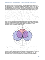
In dynamics processing, the two general possibilities are compression and expansion,
each of which can be done in the upwards or downwards direction (Figure 7.11). Generally,
compression attenuates the higher amplitudes and boosts the lower ones, the result of which is
less difference in level between the loud and quiet parts, reducing the dynamic range. Expansion
generally boosts the high amplitudes and attenuates the lower ones, resulting in an increase in
dynamic range. To be precise:
 Downward compression attenuates signals that are above a given threshold, not
changing signals below the threshold. This reduces the dynamic range.
 Upward compression boosts signals that are below a given threshold, not changing
signals above the threshold. This reduces the dynamic range.
 Downward expansion attenuates signals that are below a given threshold, not changing
signals above the threshold. This increases the dynamic range.
 Upward expansion boosts signals that are above a given threshold, not changing signals
below the threshold. This increases the dynamic range.
The common parameters that can be set in dynamics processing are the threshold, attack
time, and release time. The threshold is an amplitude limit on the input signal that triggers
compression or expansion. (The same threshold triggers the deactivation of compression or
expansion when it is passed in the other direction.) The attack time is the amount of time
allotted for the total amplitude increase or reduction to be achieved after compression or
expansion is triggered. The release time is the amount of time allotted for the dynamics
processing to be "turned off," reaching a level where a boost or attenuation is no longer being
applied to the input signal.
14
Digital Sound & Music: Concepts, Applications, & Science, Chapter 7, last updated 7/29/2013
Figure 7.11 Dynamics compression and expansion
Adobe Audition has a dynamics processor with a large amount of control. Most
dynamics processor's controls are simpler than this – allowing only compression, for example,
with the threshold setting applying only to downward compression. Audition's processor allows
settings for compression and expansion and has a graphical view, and thus it's a good one to
illustrate all of the dynamics possibilities.
Figure 7.12 shows two views of Audition's dynamics processor, the graphic and the
traditional, with settings for downward and upward compression. The two views give the same
information but in a different form.
In the graphic view, the unprocessed input signal is on the horizontal axis, and the
processed input signal is on the vertical axis. The traditional view shows that anything above
35 dBFS should be compressed at a 2:1 ratio. This means that the level of the signal above 35
dBFS should be reduced by ½ . Notice that in the graphical view, the slope of the portion of the
line above an input value of 35 dBFS is ½. This slope gives the same information as the 2:1
setting in the traditional view. On the other hand, the 3:1 ratio associated with the 55 dBFS
threshold indicates that for any input signal below 55 dBFS, the difference between the signal
and 55 dBFS should be reduced to 1/3 the original amount. When either threshold is passed
(35 or 55 dBFS), the attack time (given on a separate panel not shown) determines how long
the compressor takes to achieve its target attenuation or boost. When the input signal moves
back between the values of 35 dBFS and 55 dBFS, the release time determines how long it
takes for the processor to stop applying the compression.
15
Digital Sound & Music: Concepts, Applications, & Science, Chapter 7, last updated 7/29/2013
16
Digital Sound & Music: Concepts, Applications, & Science, Chapter 7, last updated 7/29/2013
Figure 7.12 Dynamics processing in Adobe Audition, downward and upward compression
A simpler compressor – one of the ARDOUR LADSPA plug-ins, is shown in Figure
7.13. In addition to attack, release, threshold, and ratio controls, this compressor has knee radius
and makeup gain settings. The knee radius allows you to shape the attack of the compression to
something other than linear, giving a potentially smoother transition when it kicks in. The
makeup gain setting (often called simply gain) allows you to boost the entire output signal after
all other processing has been applied.
17
Digital Sound & Music: Concepts, Applications, & Science, Chapter 7, last updated 7/29/2013
Figure 7.13 SC1 Compressor plug-in for Ardour
7.1.9.2
Limiting and Gating
A limiter is a tool that prevents the amplitude of a signal from
going over a given level. Limiters are often applied on the
 Aside: A limiter could
be thought of as a
master bus, usually post-fader. Figure 7.14 shows the LADSPA
compressor with a
Fast Lookahead Limiter plug-in. The input gain control allows
compression ratio of
you to increase the input signal before it is checked by the
infnity to 1. See the
next section on
limiter. This limiter looks ahead in the input signal to determine
dynamics compression.
if it is about to go above the limit, in which case the signal is
attenuated by the amount necessary to bring it back within the
limit. The lookahead allows the attenuation to happen almost instantly, and thus there is no
attack time. The release time indicates how long it takes to go back to 0 attenuation when
limiting the current signal amplitude is no longer necessary. You can watch this work in realtime by looking at the attenuation slider on the right, which bounces up and down as the limiting
is put into effect.
Figure 7.14 Limiter LADSPA plug-in
A gate allows an input signal to pass through only if it is above a certain threshold. A
hard gate has only a threshold setting, typically a level in dB above or below which the effect is
engaged. Other gates allow you to set an attack, hold, and release time to affect the opening,
holding, and closing of the gate (Figure 7.16). Gates are sometimes used for drums or other
18
Digital Sound & Music: Concepts, Applications, & Science, Chapter 7, last updated 7/29/2013
instruments to make their attacks appear sharper and reduce the bleed from other instruments
unintentionally captured in that audio signal.
Figure 7.15 Gate (Logic Pro)
A noise gate is a specially designed gate that is intended to reduce the extraneous noise
in a signal. If the noise floor is estimated to be, say, 80 dBFS, then a threshold can be set such
that anything quieter than this level will be blocked out, effectively transmitted as silence. A
hysteresis control on a noise gate indicates that there is a threshold difference between opening
and closing the gate. In the noise gate in Figure 7.16, the threshold of 50 dB and the hysteresis
setting of 3 dB indicate that the gate closes at 50 dBFS and opens again at 47 dBFS. The
side chain controls allow some signal other than the main input signal to determine when the
input signal is gated. The side chain signal could cause the gate to close based on the amplitudes
of only the high frequencies (high cut) or low frequencies (low cut).
In a practical sense, there is no real difference between a gate and a noise gate. A
common misconception is that noise gates can be used to remove noise in a recording. In reality
all they can really do is mute or reduce the level of the noise when only the noise is present.
Once any part of the signal exceeds the gate threshold, the entire signal is allowed through the
gate, including the noise. Still, it can be very effective at clearing up the audio in between words
or phrases on a vocal track, or reducing the overall noise floor when you have multiple tracks
with active regions but no real signal, perhaps during an instrumental solo.
19
Digital Sound & Music: Concepts, Applications, & Science, Chapter 7, last updated 7/29/2013
Figure 7.16 Noise gate (Logic Pro)
7.2 Applications
7.2.1 Mixing
7.2.1.1
Mixing Contexts and Devices
A mixing console, or mixer, is a device that
 Aside: The fact that digital consoles often
takes several different audio signals and mixes
follow analog models of control and layout is
them together, typically to be sent to another
somewhat of a hot topic. On one hand, this
device in a more consolidated or organized
similarity provides some standardization and
ease of transition between the two types of
manner. Mixing can be done in a variety of
consoles. Yet with all of the innovations in user
contexts. Mixing during a live performance
interface technology, you might wonder why
requires that an audio engineer balance the
these implementations have remained so “old
sounds from a number of sources. Mixing is
fashioned.” Many people are beginning to use
hi-tech UI devices like the iPad along with
also done in the sound studio, as the recordings
wireless control protocols like OSC to reinvent
from multiple channels or on multiple tracks are
the way mixing and audio manipulation is done.
combined.
While it may take some time for these new
Mixing can also be done with a variety of
techniques to emerge and catch on, the
possibilities they provide are both fascinating
tools. An audio engineering doing the mixing of
and seemingly limitless.
a live performance could use a hardware device
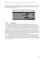
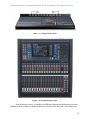
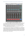
like the one shown in Figure 7.17, an analog
mixing console. Digital mixers have now become
more common (Figure 7.18), and as you can see, they look pretty much the same as their analog
counterparts. Software mixers, with user interfaces modeled after equivalent hardware, are a
standard part of audio processing programs like Pro Tools, Apple Logic, Ableton Live, and
Cakewalk Sonar. The mixing view for a software mixer is sometimes called the console view, as
is the case with Cakewalk Sonar, pictured in Figure 7.19.
20
Digital Sound & Music: Concepts, Applications, & Science, Chapter 7, last updated 7/29/2013
Figure 7.17 Analog mixing console
Figure 7.18 A digital mixing console
In the following section, we introduce the different components and functions of mixers.
Whether a mixer is analog or digital, hardware or software, is not the point. The controls and
21
Digital Sound & Music: Concepts, Applications, & Science, Chapter 7, last updated 7/29/2013
functions of mixers are generally the same no matter what type you're dealing with or the context
in which you're doing the mixing.
Practical
Exercise:
Mixing MultiTrack Audio
Figure 7.19 Console view (mixing view) in Cakewalk Sonar
22
Digital Sound & Music: Concepts, Applications, & Science, Chapter 7, last updated 7/29/2013
7.2.1.2
Inputs and Outputs
The original concept behind a mixer was to take the signals from multiple sources and combine
them into a single audio signal that could be sent to a recording device or to an amplification
system in a performance space. These so-called “mix down” consoles would have several audio
input connections but very few output connections. With the advent of surround sound,
distributed sound reinforcement systems, multitrack recorders, and dedicated in-ear monitors,
most modern mixing consoles have just as many, if not more, outputs than inputs, allowing the
operator to create many different mixes that are delivered to different destinations.
Consider the situation of a recording session of a small rock band. You could easily have
more than twenty-four microphones spread out across the drums, guitars, vocalists, etc. Each
microphone connects to the mixing console on a separate audio input port and is fed into an
input channel on the mixing console. Each channel has a set of controls that allows you to
optimize and adjust the volume level and frequency response of the signal and send that signal to
several output channels on the mixing console. Each output channel represents a different mix
of the signals from the various microphones. The main mix output channel likely contains a mix
of all the different microphones and is sent to a pair (or more) of monitor loudspeakers in the
control room for the recording engineer and other participants to listen to the performance from
the band. This main mix may also represent the artistic arrangement of the various inputs,
decided upon by the engineer, producer, and band members, eventually intended for mixed-down
distribution as a stereo or surround master audio file. Each performer in the band is also often
fed a separate auxiliary output mix into her headphones. Each auxiliary mix contains a custom
blend of the various instruments that each musician needs to hear in order to play his part in time
and in tune with the rest of the band. Ideally, the actual recording is not a mix at all. Instead, each
input channel has a direct output connection that sends the microphone signal into a dedicated
channel on a multitrack recording device, which in the digital age is often a dedicated computer
DAW. This way the raw, isolated performances are captured in their original state, and the
artistic manipulation of the signals can accomplished incrementally and non-destructively during
the mixing process.
7.2.1.3
Channel Strips
Configuring all the knobs, buttons, and faders on a suitably sized mixing console makes all of the
above functions possible. When you see a large mixing console like the one pictured in Figure
7.17, you might feel intimidated by all the knobs and buttons. It’s important to realize that most
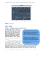
of the controls are simply duplicates. Each input channel is represented by a vertical column, or
channel strip, of controls as shown in Figure 7.20.
It’s good to realize that the audio signal typically travels through the channel strip and its
various controls from top to bottom. This makes it easy to visualize the audio signal path and
understand how and when the audio signal is being affected. For example, you’ll typically find
the preamp gain control at the top of the channel strip, as this is the first circuit the audio signal
encounters, while the level fader at the bottom is the last component the signal hits as it leaves
the channel strip to be mixed with the rest of the individual signals.
23
Digital Sound & Music: Concepts, Applications, & Science, Chapter 7, last updated 7/29/2013
Figure 7.20 A single channel strip from an analog mixing console
24
Digital Sound & Music: Concepts, Applications, & Science, Chapter 7, last updated 7/29/2013
7.2.1.4
Input Connectors
Each input channel has at least one input connector, as shown in Figure 7.21. Typically this is an
XLR connector. Some mixing consoles also have a ¼" TRS connector on each input channel.
The idea for including both is to use the XLR connector for microphone signals and the ¼"
connector for line level or high impedance instrument signals, though you can’t use both at the
same time. In most cases, both connectors feed into the same input circuitry, allowing you to use
the XLR connector for line level signals as well as microphone signals. This is often desirable,
and whenever possible you should use the XLR connector rather than the ¼" because of its
benefits such as a locking connection. In some cases, the ¼" connector feeds into the channel
strip on a separate path from the XLR connector, bypassing the microphone preamplifier or
encountering a 20 dB attenuation before entering the preamplifier. In this situation, running a
line level signal through the XLR connector may result in a clipped signal because there is no
gain adjustment to compensate for the increased voltage level of the line level signal. Each
mixing console implements these connectors differently, so you’ll need to read the manual to
find out the specific configuration and input specifications for your mixing console.
Figure 7.21 Input connectors for a single channel on a mixing console
7.2.1.5
Gain Section
The gain section of the channel strip includes several controls. The most important is the gain
knob. Sometimes labeled trim, this knob controls the preamplifier for the input channel. The
preamplifier is an electrical circuit that can amplify the incoming audio signal to the optimal line
level voltage suitable for use within the rest of the console. The preamplifier is often designed
for high quality and very low noise so that it can boost the audio signal without adding a lot of
25
Digital Sound & Music: Concepts, Applications, & Science, Chapter 7, last updated 7/29/2013
noise or distortion. Because of the sheer number of electrical circuits an audio signal can pass
through in a mixing console, the signal can pick up a lot of noise as it travels around in the
console. The best way to minimize the effects of this noise is to increase the signal-to-noise
ratio from the very start. Since the preamplifier is able to increase the level of the incoming
audio signal without increasing the noise level in the console, you can use the preamplifier to
increase the ratio between the noise floor of the mixing console and the level of your audio
signal. Therefore, the goal of the gain knob is to achieve the highest value possible without
clipping the signal.
Figure 7.22 Gain section of an input channel strip
This is the only place in the console (and likely your entire sound system) where you can
increase the level of the signal without also increasing the noise. Thus, you should get all the
gain you can at this stage. You can always turn the level down later in the signal chain. Don’t
succumb to the temptation to turn down the mixing console preamplifier as a convenient way to
fix problems caused downstream by power amplifiers and loudspeakers that are too powerful or
too sensitive for your application. Also, you should not turn down the preamplifier in an effort to
get all the channel faders to line up in a straight row. These are excellent ways to create a noisy
sound system because you're decreasing the signal-to-noise ratio for the incoming audio signal.
Once you’ve set that gain knob to the highest level you can without clipping the signal, the only
reason you should ever touch it again is if the signal coming in to the console gets louder and
starts clipping the input.
If you're feeding a line level signal into the channel, you might find that you're clipping
the signal even though the gain knob is turned all the way down. Most mixing consoles have a
pad button next to the gain knob. This pad button (sometimes labeled “20 dB”, “Line”, “range”
or “Mic/Line”) will attenuate the signal by 20 dB, which should allow you to find a setting on
your gain knob that doesn’t clip. Using the pad button shouldn’t necessarily be something you do
automatically when using line level signals, as you’re essentially undoing 20 dB of built-in
signal-to-noise ratio. Don’t use it unless you have to. Be aware that sometimes this button also
serves to reroute the input signal using the ¼" input instead of the XLR. On some consoles that
26
Digital Sound & Music: Concepts, Applications, & Science, Chapter 7, last updated 7/29/2013
have both ¼" and XLR inputs yet don’t have a pad button, it’s because the 20 dB attenuation is
already built in to the signal chain of the ¼" input. These are all factors to consider when
deciding how to connect your equipment to the mixing console.
Another button you'll commonly find next to the gain knob is labeled Ø. This is probably
the most misunderstood button in the world of sound. Unfortunately, the mixing console
manufacturers contribute to the confusion by labeling this button with the universal symbol for
phase. In reality, this button has nothing to do with phase. This is a polarity button. Pressing
this button will simply invert the polarity of your signal.
The badly-chosen symbol for the polarity button is inherited from the general confusion
among sound practitioners about the difference between phase and polarity. It's true that for pure
sine waves, a 180-degree phase shift is essentially identical to a polarity inversion. But that's the
only case where these two concepts intersect. In the real world of sound, pure sine waves are
hardly ever encountered. For complex sounds that you will deal with in practice, phase and
polarity are fundamentally different. Phase changes in complex sounds are typically the result of
an offset in time. The phase changes as a result of timing offsets are not consistent across the
frequency spectrum. A shift in time that would create a 180-degree phase offset for 1 kHz would
create a 360-degree phase offset for 2 kHz. This inconsistent phase shift across the frequency
spectrum for complex sounds is the cause of comb filtering when two identical sounds are mixed
together with an offset in time. Given that a mixing console is all about mixing sounds, it is very
easy to cause comb filtering when mixing two microphones that are picking up the same sound at
two different distances resulting in a time offset. If you think the button in question adjusts the
phase of your signal (as the symbol on the button suggests), you might come to the conclusion
that pressing this button will manipulate the timing of your signal and compensate for comb filter
problems. Nothing could be further from the truth. In a comb filter situation, pressing the polarity
button for one of the two signals in question will simply convert all cancelled frequencies into
frequencies that reinforce each other. All the frequencies that were reinforcing each other will
now cancel out. Once you’ve pressed this button, you still have a comb filter. It’s just an inverted
comb filter. When you encounter two channels on your console that cause a comb filter when
mixed together, a better strategy is to simply eliminate one of the two signals. After all, if these
two signals are identical enough to cause a comb filter, you don’t really need both of them in
your mix, do you? Simply ducking the fader on one of the two channels will solve your comb
filter problem much more efficiently, and certainly more so than using the polarity button.
If this button has nothing to do with phase, what reason could you possibly have to push
it? There are many situations where you might run into a polarity problem with one of your input
signals. The most common is the dreaded “pin 3 hot” problem. In Chapter 1, we talked about the
pinout for an XLR connector. We said that pin 2 carries the positive or “hot” signal and pin 3
carries the negative or “cold” signal. This is a standard from the Audio Engineering Society that
was ratified in 1982. Prior to that, each manufacturer did things differently. Some used pin 2 as
hot and some used pin 3 as hot. This isn’t really a problem until you start mixing and matching
equipment from different manufacturers. Let’s assume your microphone uses pin 2 as hot, but
your mixing console uses pin 3 as hot. In that situation, the polarity of the signal coming into the
mixing console is inverted. Now if you connect another microphone to a second channel on your
mixing console and that microphone also uses pin 3 as hot, you have two signals in your mixing
console that are running in opposite polarity. In these situations, having a polarity button on each
channel strip is an easy way to solve this problem. Despite the pin 2 hot standard being now
thirty years old, there are still some manufacturers making pin-3-hot equipment.
27
Digital Sound & Music: Concepts, Applications, & Science, Chapter 7, last updated 7/29/2013
Even if all your equipment is running pin 2 hot, you could still have a polarity inversion
happening in your cables. If one end of your cable is accidentally wired up incorrectly (it
happens more often than you might think), you could have a polarity inversion when you use that
cable. You could take the time to re-solder that connector (which you should ultimately take care
of), but if time is short or the cable is hard to get to, you could simply press the polarity button
on the mixing console and instantly solve the problem.
There could be artistic reasons you would want to press the polarity button. Consider the
situation where you are trying to capture the sound of a drum. If you put the microphone over the
top of the drum, when the drum is hit, the diaphragm of the microphone pulls down towards the
drum. When this signal passes through your mixing console on to your loudspeakers, the
loudspeaker driver also pulls back away from you. Wouldn’t it make more sense for the
loudspeaker driver to jump out towards you when the drum is hit? To solve this problem you
could go back to the drummer and move the microphone so it sits underneath the drum, or you
could save yourself the trip and just press the polarity button. The audible difference here might
be subtle, but when you put enough subtle differences together, you can often get a significant
difference in audio quality.
Another control commonly found in the gain section is the phantom power button.
Phantom power is a 48-volt electrical signal that is sent down the shield of the microphone cable
to power condenser microphones. In our example, there is a dedicated 48-volt phantom power
button for each input channel strip. In some consoles, there's a global phantom power button that
turns on phantom power for all inputs.
The last control that is commonly found in the gain section of the console is a high-pass
filter. Pressing this button filters out frequencies below the cutoff frequency for the filter.
Sometimes this button has a fixed cutoff frequency of 80Hz, 100Hz, or 125Hz. Some mixing
consoles give you a knob along with the button that allows you to set a custom cutoff frequency
for the high pass filter. When working with microphones, it's very easy to pick up unwanted
sounds that have nothing to do with the sound you’re trying to capture. Footsteps, pops, wind,
and handling noise from people touching and moving the microphone are all examples of
unwanted sounds that can show up in your microphone. The majority of these sounds fall in very
low frequencies. Most musical instruments and voices do not generate frequencies below 125
Hz, so you can safely use a high-pass to filter out frequencies lower than that. Engaging this
filter removes most of these unwanted sounds before they enter the signal chain in your system
without affecting the good sounds you’re trying to capture. Still, all filters have an effect on the
phase of the frequencies surrounding the cutoff frequency, and they can introduce a small
amount of additional noise into the signal. For this reason, you should leave the high-pass filter
disengaged unless you need it.
7.2.1.6
Insert
Next to the channel input connectors typically there is a set of insert connections. Insert
connections consist of an output and input that allow you to connect some kind of external
processing device in line with the signal chain in the channel strip. The insert output typically
takes the audio signal from the channel directly after it exits the preamplifier, though some
consoles let you choose at what point in the signal path the insert path lies. Thinking back to the
top-down signal flow, the insert connections are essentially “inserting” an extra component at
that point on the channel strip. In this case, the component isn’t built into the channel strip like
the EQ or pan controls. Rather, the device is external and can be whatever the engineer wishes
28
Digital Sound & Music: Concepts, Applications, & Science, Chapter 7, last updated 7/29/2013
to use. If, for example, you want to compress that dynamics of the audio on input channel 1, you
can connect the insert output from channel 1 to the input of an external compressor. Then the
output of the compressor can be connected to the insert input on channel 1 of the mixing console.
The compressed signal is then fed back into the channel strip and continues down the rest of the
signal chain for channel 1. If nothing is connected to the insert ports, it is bypassed and the signal
is fed directly through the internal signal chain for that input channel. When you connect a cable
to the insert output, the signal is almost always automatically rerouted away from the channel
strip. You’ll need to feed something back into the insert input in order to continue using that
channel strip on the mixing console.
There are two different connection designs for inserts on a mixing console. The ideal
design is to have a separate ¼" or XLR connection for both the insert output and input. This
allows you to use standard patch cables to connect the external processing equipment, and may
also employ a balanced audio signal. If the company making the mixing console needs to save
space or cut down on the cost of the console, they might decide to integrate both the insert output
and input on a single ¼" TRS connector. In this case, the input and output are handled as
unbalanced signals using the tip for one signal, the ring for the other signal, and a shared neutral
on the sleeve. There is no standard for whether the input or output is carried on the tip vs. the
ring. To use this kind of insert requires a special cable. This cable has three connectors. On one
end is a ¼" TRS connector. This connector has two cables coming out of the end. One cable
feeds an XLR male or a ¼" TS connector for the insert output and a XLR female or a ¼" TS
connector for the insert input.
7.2.1.7
Equalizer Section
After the gain section of the channel strip, the next section your audio signal encounters is the
equalizer section (EQ) shown in Figure 7.23. The number of controls you see in this section of
the channel strip varies greatly across the various models of mixing consoles. Very basic
consoles may not include an EQ section at all. Generally speaking, the more money you pay for
the console, the more knobs and buttons you find in the EQ section. We discussed the
equalization process in depth in Chapter 7.
29
Digital Sound & Music: Concepts, Applications, & Science, Chapter 7, last updated 7/29/2013
Figure 7.23 EQ section of an input channel strip
Even the simplest of mixing consoles typically has two channels of EQ in each channel
strip. These are usually a high shelf and a low shelf filter. These simple EQ sections consist of
two knobs. One controls the gain for the high shelf and the other for the low shelf. The shelving
frequency is a fixed value. If you pay a little more for your mixing console, you can get a third
filter – a mid-frequency peak-notch filter. Again, the single knob isa gain knob with a fixed
center frequency and bandwidth.
The next controllable parameter you’ll get with a nicer console is a frequency knob.
Sometimes only the mid-frequency notch filter gets the extra variable center frequency knob, but
the high and low shelf filters may get a variable filter frequency using a second knob as well.
With this additional control, you now have a semi-parametric filter. If you are given a third knob
to control the filter Q or Bandwidth, the filter becomes fully parametric. From there you simply
get more bands of fully parametric filters per channel strip as the cost of the console increases.
Depending on your needs, you may not require five bands of EQ per channel strip. The
option that is absolutely worth paying for is an EQ bypass button. This button routes the audio
signal in the channel around the EQ circuit. This way, the audio signal doesn’t have to be
processed by the EQ if you don’t need any adjustments to the frequency response of the signal.
Routing around the EQ solves two potential problems. The first is the problem of inheriting
someone else’s solution. There are a lot of knobs on a mixing console, and they aren’t always
30
Digital Sound & Music: Concepts, Applications, & Science, Chapter 7, last updated 7/29/2013
reset when you start working on a new project. If the EQ settings from a previous project are still
dialed in, you could be inheriting a frequency adjustment that's not appropriate for your project.
Having an EQ bypass button is a quick way to turn off all the EQ circuits so you're starting with
a clean slate. The bypass button can also help you quickly do an A/B comparison without having
to readjust all of the filter controls. The second problem is related to noise floor. Even if you
have all the EQ gain knobs flattened out (no boost or cut), your signal is still passing though all
those circuits and potentially collecting some noise along the way. Bypassing the EQ allows you
to avoid that unnecessary noise.
7.2.1.8
Auxiliaries
The Auxiliary controls in the channel strip are shown in Figure 7.24. Each auxiliary send knob
represents an additional physical audio path/output on the mixing console. As you increase the
value of an auxiliary send knob, you're setting a certain level of that channel’s signal to be sent
into that auxiliary bus. As each channel is added into the bus to some degree, a mix of those
sounds is created and sent to a physical audio output connected to that bus. You can liken the
function of the auxiliary busses to an actual bus transportation system. Each bus, or bus line,
travels to a unique destination, and the send knob controls how much of that signal is getting on
the bus to go there. In most cases, the mixing console will also have a master volume control to
further adjust the combined signal for each auxiliary output. This master control can be a fader or
a knob and is typically located in the central control section of the mixing console.
An auxiliary is typically used whenever you need to send a unique mix of the various
audio signals in the console to a specific device or person. For example, when you record a band,
the lead singer wears headphones to hear the rest of the band as well as her own voice. Perhaps
the guitar is the most important instrument for the singer to hear because the guitar contains the
information about the right pitch the singer needs to use with her voice. In this situation, you
would connect her headphones to a cable that is fed from an auxiliary output, which we'll call
“Aux 1,” on the mixing console. You might dial in a bit of sound to Aux 1 across each input
channel of the mixing console, but on the channels containing the guitar and the singer’s own
vocals the Aux 1 controls would be set to a higher value so they're louder in the mix being sent
to the singer’s headphones.
31
Digital Sound & Music: Concepts, Applications, & Science, Chapter 7, last updated 7/29/2013
Figure 7.24 Auxiliary section of input channel strip
The auxiliary send knobs on an input channel strip come in two configurations. PreFader aux sends send signal level into the aux bus independently of the position of the channel
fader. In our example of the singer in the band, a pre-fade aux would be desirable because once
you've dialed in an aux mix that works for the singer, you don’t want that mix changing every
time you adjust the channel fader. When you adjust the channel fader, it's in response to the main
mix that is heard in the control room, which has no bearing on what the singer needs to hear.
The other configuration for an aux send is Post-Fader. In this case, dialing in the level on
the aux send knob represents a level relative to the fader position for that input channel. So when
the main mix is changed via the fader, the level in that aux send is changed as well. This is
particularly useful when you're using an aux bus for some kind of effect processing. In our same
recording session example, you might want to add some reverberation to the mix. Instead of
inserting a separate reverb processor on each input channel, requiring multiple processors, it's
much simpler to connect an aux output on the mixing console to the input of a single reverb
processor. The output of the reverb processor then comes back into an unused input channel on
the mixing console. This way, you can use the aux sends to dial in the desired amount of reverb
for each input channel. The reverb processor then returns a reverberant mix of all of the sounds
that gets added into the main mix. Once you get a good balance of reverb dialed in on an aux
send for a particular input channel, you don’t want that balance to change. If the aux send to the
reverb is pre-fader, when the fader is used to adjust the channel level within the main mix, the
32
Digital Sound & Music: Concepts, Applications, & Science, Chapter 7, last updated 7/29/2013
reverb level remains the same, disrupting the balance you achieve. Instead, when you turn up or
down the channel fader, the level of the reverb should also increase or decrease respectively so
the balance between the dry and the reverberant (wet) sound stays consistent. Using a post-fader
aux send accomplishes this goal.
Some mixing consoles give you a switch to change the behavior of an aux bus between
pre-fader and post-fader, while in other consoles this behavior may be fixed. Sometimes this
switch is located next to the aux master volume control, and changes the pre-fader or post-fader
mode for all of the channel aux sends that feed into that bus. More expensive consoles allow you
to select pre- or post-fader behavior in a channel-specific way. In other words, each individual
aux send dial on an input channel strip has its own pre- or post-fade button. With this flexibility
Aux 1 can be set as a pre-fade aux for input channel 1 and a post-fade aux for input channel 2.
7.2.1.9
Fader and Routing Section
The fader and routing section shown in Figure 7.25 is where you usually spend most of your time
working with the console in an iterative fashion during the artistic process of mixing. The fader
is a vertical slider control that adjusts the level of the audio signal sent to the various mixes
you've routed on that channel. There are two common fader lengths: 60 mm and 100 mm. The
100 mm faders give your fingers greater range and control and are easier to work with. The fader
is primarily an attenuator. It reduces the level of the signal on the channel. Once you've set the
optimal level for the incoming signal with the preamplifier, you use the fader to reduce that level
to something that fits well in the mix with the other sounds. The fader is a very low-noise circuit,
so you can really set it to any level without having adverse effects on signal-to-noise ratio. One
way to think about it is that the preamplifier is where the science happens; the fader is where the
art happens. The fader can reduce the signal level all the way to nothing (−∞ or –inf), but
typically has only five to ten dB on the amplification end of the level adjustment scale. When the
fader is set to 0 dB, also referred to as unity, the audio signal passes through with no change in
level. You should set the fader level to whatever sounds best, and don’t be afraid to move it
around as the levels change over time.
33
Digital Sound & Music: Concepts, Applications, & Science, Chapter 7, last updated 7/29/2013
Figure 7.25 Fader and routing section of an input channel strip
Near the fader there is usually a set of signal routing buttons. These buttons route the
audio signal at a fixed level relative to the fader position to various output channels on the
34
Digital Sound & Music: Concepts, Applications, & Science, Chapter 7, last updated 7/29/2013
mixing console. There is almost always a main left and right stereo output (labeled “MIX” in
Figure 7.25), and sometimes a mono or center output. Additionally, you may also be able to
route the signal to one or more group outputs or subgroup mixes. A subgroup (sometimes as
with auxiliaries also called a bus) represents a mixing channel where input signals can be
grouped together under a master volume control before being passed on to the main stereo or
mono output, as shown in Figure 7.26. An example of subgroup routing would be to route all the
drum microphones to a subgroup so you can mix the overall level of the drums in the main mix
using only one fader. A group is essentially the same thing, except it also has a dedicated
physical output channel on the mixing console. The terms bus, group, and subgroup are often
used interchangeably. Group busses are almost always post fader, and unlike auxiliary busses
don't have variable sends – it’s all or nothing. Group routing buttons are often linked in stereo
pairs, where you can use the pan knob to pan the signal between the paired groups, in addition to
panning between the main stereo left and right bus.
Figure 7.26 Master control section of an analog mixing console
35
Digital Sound & Music: Concepts, Applications, & Science, Chapter 7, last updated 7/29/2013
Also near the fader you usually have a mute button. The mute button mimics the
behavior of pulling the input fader all the way down. In this case, pre-fade auxiliaries would
continue to function. The mute button comes in handy when you want to stop hearing a
particular signal in the main mix, but you don’t want to lose the level you have set on the fader
or lose any auxiliary functionality, like signal being sent a headphone or monitor mix. Instead of
a mute button, you may see an on/off button. This button shuts down the entire channel strip. In
that situation, all signals stop on the channel, including groups, auxiliaries, and direct outs. Just
to confuse you, manufacturers may use the terms mute and on/off interchangeably so in some
cases, a mute button may behave like an on/off button and vice versa. Check the user manual for
the mixing console to find out the exact function of your button.
Next to the fader there is typically be a pre-fade listen (PFL) or a solo button. Pressing
the PFL button routes the signal in that channel strip to a set of headphones or studio monitor
outputs. Since it is pre-fade, you can hear the signal in your headphones even if the fader is down
or the mute button is pressed. This is useful when you want to preview the sound on that channel
before you allow it to be heard via your main or group outputs. If you have a solo button, when
pressed it will also mute all the other channels, allowing you to hear only the solo-enabled
channels. Solo is typically found in recording studio consoles or audio recording software.
Sometimes the terms PFL and solo are used interchangeably so, again, check the user manual for
your mixing console to be sure of the function for this button.
Similar to PFL is after-fade listen (AFL). AFL is typically found on output faders
allowing you to preview in your headphones the signal that is passing through a subgroup, group,
aux, or main output. The after-fade feature is important because it allows you to hear exactly
what is passing through the output, including the level of the fader. For example, if a musician
says that he can’t hear a given instrument in his monitor, you can use the AFL feature for the aux
that feeds that monitor to see if the instrument can be heard. If you can hear it in your
headphones, then you know that the aux is functioning properly. In this case, you may need to
adjust the mix in that aux to allow the desired instrument to be heard more easily. If you can't
hear the desired instrument in your headphones, then you know that you have a routing problem
in the mixing console that's preventing the signal from sending out from that aux output.
Depending on the type of mixing console you're using, you may also have some sort of
PPM (Peak Programme Meter) near the fader. In some cases, this will be at the top of the
console on a meter bridge. Cheaper consoles will just give you two LED indicators, one for when
audio signal is present and another for when the signal clips. More expensive consoles will give
you high-resolution PPMs with several different level indicators. A PPM is more commonly
found in digital systems, but is also used in analog equipment. A PPM is typically a long column
of several LED indicators in three different colors, as shown in Figure 7.27. One color represents
signal levels below the nominal operating level, another color represents signals at or above
nominal level, and the third color (usually red) represents a signal that is clipping or very near to
clipping. A PPM responds very quickly to the audio signal. Therefore, a PPM is very useful for
measuring peak values in an audio signal. If you’re trying to find the right position for a
preamplifier, a PPM will show you exactly when the signal clips. Most meters in audio software
are programmed to behave like a PPM.
36
Digital Sound & Music: Concepts, Applications, & Science, Chapter 7, last updated 7/29/2013
Hardware PPM meter
Software PPM meter
Figure 7.27 PPM meters
7.2.2
Applying EQ
An equalizer can be incredibly useful when used appropriately, and incredibly
dangerous when used inappropriately. Knowing when to use an EQ is just as
important and knowing how to use it to accomplish the effect you are looking
for. Every time you think you want to use an EQ you should evaluate the
situation against this rule of thumb: EQ should be used to create an effect, not to
Max Demo:
solve a problem. Using an EQ as a problem solver can cause new problems
Equalization
when you should really just figure out what’s causing the original problem and
fix that instead. Only if the problem can’t be solved in any other way should
you pull up the EQ, perhaps if you’re working post-production on a recording captured earlier
during a film shoot, or you’ve run into an acoustical issue in a space that can’t be treated or
physically modified. Rather than solving problems, you should try to use an EQ as a tool to
achieve a certain kind of sound. Do you like your music to be heavy on the bass? An EQ can
help you achieve this. Do you really like to hear the shimmer of the cymbals in a drum set? An
EQ can help.
Let’s examine some common problems you may encounter where you will be tempted to
use an EQ inappropriately. As you listen to the recording you’re making of a singer you notice
that the recorded audio has a lot more low frequency content than high frequency content,
leading to a decreased intelligibility. You go over and stand next to the performer to hear what
they actually sound like and notice that they sound quite different than what you are hearing
from the microphone. Standing next to them you can hear all those high frequencies quite well.
In this situation you may be tempted to pull out your EQ and insert a high shelf filter to boost all
those high frequencies. This should be your last resort. Instead, you might notice that the singer
is singing into the side of the microphone instead of the front. Because microphones are more
directional at high frequencies than low frequencies, singing into the side of the microphone
37
Digital Sound & Music: Concepts, Applications, & Science, Chapter 7, last updated 7/29/2013
would mean that the microphone picks up the low frequency content very easily but the high
frequencies are not being captured very well. In this case you would be using an EQ to boost
something that isn’t being picked up very well in the first place. You will get much better results
by simply rotating the microphone so it is pointed directly at the singer so the singer is singing
into the part of the microphone that is more sensitive to high frequencies.
Another situation you may encounter would be when mixing the sound from multiple
microphones either for a live performance or a recording. You notice as you start mixing
everything together that a certain instrument has a huge dip around 250 Hz. You might be
tempted to use an EQ to increase 250 Hz. The important thing to keep in mind here is that most
microphones are able to pick up 250 Hz quite well from every direction, and it is unlikely that
the instrument itself is somehow not generating the frequencies in the 250 Hz range while still
generating all the other frequencies reasonably well. So before you turn on that EQ, you should
mute all the other channels on the mixer and listen to the instrument alone. If the problem goes
away, you know that whatever is causing the problem has nothing to do with EQ. In this
situation, comb filtering is the likely culprit. There’s another microphone in your mix that was
nearby and happened to be picking up this same instrument at a slightly longer distance of about
two feet. When you mix these two microphones together, 250 Hz is one of the frequencies that
cancels out. If that isn’t the issue, try moving a foot or two closer to or farther away from the
loudspeakers. If the 250 Hz dip goes away in this case, there’s likely a standing wave resonance
in your studio at the mix position that is cancelling out this frequency. Using an EQ in this case
will not solve the problem since you’re trying to boost something that is actively being cancelled
out. A better solution for the standing wave would be to consider rearranging your room or
applying acoustical treatment to the offending surfaces that are causing this reflective build up.
If comb filtering was the issue, you should try to better isolate the signals either by moving the
microphones farther apart or preventing them from being summed together in the mix. A gate
might come in handy here too. If you gate both signals you can minimize the times when both
microphones are mixed together, since the signals won’t be let through when the instruments
they are being used for aren’t actually playing.
Suppose you are operating a sound reinforcement system for a live performance and you
start getting feedback through the sound system. When you hear that single frequency start it’s
endless loop through the system you might be tempted to use an EQ to pull that frequency out of
the mix. This will certainly stop the feedback, but all you really get is the ability to turn the
system up another decibel or so before another frequency will inevitably start to feed back.
Repeat the process a few times and in no time at all you will have completely obliterated the
frequency response of your sound system. You won’t have feedback, but the entire system will
sound horrible. A better strategy for solving this problem would be to get the microphone closer
to the performer, and move the performer and the microphone farther away from the
loudspeakers. You’ll get more gain this way and you can maintain the frequency response of
your system.
We could examine many more examples of an inappropriate use of an EQ but they all go
back to the rule of thumb regarding the use of an EQ as a problem solver. In most cases, an EQ is
a very ineffective problem solver. It is, however, a very effective tool for shaping the tonal
quality of a sound. This is an artistic effect that has little to do with problems of a given sound
recording or reinforcement system. Instead you are using the EQ to satisfy a certain tonal
preference for the listener. These effects could be as subtle as reducing an octave band of
frequencies around 500 Hz by -3 dB to achieve more intelligibility for the human voice by
38
Digital Sound & Music: Concepts, Applications, & Science, Chapter 7, last updated 7/29/2013
allowing the higher frequencies to be more prominent. The effect could be as dramatic as using a
band pass filter to mimic the effect of a small cheap loudspeaker in a speakerphone. When using
an EQ as an effect, keep in mind another rule of thumb. When using an EQ you should reduce
the frequencies that are too loud instead of increasing the frequencies that are too quiet. Every
sound system, whether in a recording studio or a live performance, has an amplitude ceiling; the
point at which the system clips and distorts. If you’ve done your job right, you will be running
the sound system at an optimal gain, and a 3 dB boost of a given frequency on an EQ could be
enough to cause a clipped signal. Reducing frequencies is always safer than boosting them since
reducing them will not blow the gain structure in your signal path.
7.2.3
Applying Reverb
Almost every audio project you do will likely benefit from some reverb processing. In a practical
sense, most of the isolation strategies we use when recording sounds will have a side effect of
stripping the sound of natural reverberation. So anything recorded in a controlled environment
such as a recording studio will probably need some reverb added to make it sound more natural.
There are varying opinions on this among
audio professionals. Some argue that
 Aside: In an attempt to reconcile these two
artificial reverberation processers are
schools of thought on reverberation in the
sounding quite good now, and since it is
recording studio, some have resorted to installing
impossible to remove natural
active acoustic systems in the recording studio.
These systems involve placing microphones
reverberation from a recording, it makes
throughout the room that feed into live digital
more sense to capture your recorded
signal processors that generate thousands of
audio as dry as possible. This way
delayed sounds that are then sent into several
loudspeakers throughout the room. This creates a
you’re able to artificially add back
natural-sounding artificial reverb that is captured in
whatever reverberation you need in a
the recording the same as natural reverb. The
way that you can control. Others argue
advantage here is that you can change the reverb
that having musicians perform in an
by adjusting the parameters of the DSP for
different recording situations. To hear an example
acoustically dry and isolated
of this kind of system in action, see this video from
environment will negatively impact the
TRI Studios where Bob Weir from the Grateful
quality of their performance. Think
Dead has installed an active acoustic system in his
about how much more confident you
recording studio.
feel when singing in the shower. All that
reverberation from the tiled surfaces in the
shower create a natural reverberation that makes your voice sound better to you than normal.
That gives you the confidence to sing in a way that you probably don’t in public. So some
recording engineers would prefer to have some natural reverberation in the recording room to
help the musicians to deliver a better performance. If that natural reverberation is well controlled
acoustically you could even end up with a recording that sounds pretty good already and might
require minimal additional processing.
Regardless of the amount of reverb you already have in your recording, you will likely
still want to add some artificial reverb to the mix. There are three places you can apply the reverb
in your signal chain. You can set it up as an insert for a specific channel in a multi-channel mix.
In this case the reverb only gets applied to the one specific channel and the other channels are
left unchanged. You will have to adjust the wet/dry mix in the reverb processor to create an
appropriate balance. This technique can be useful for a special effect you want to put on a
specific sound, but using this technique on every channel in a large multi-channel mix will cost
39
Digital Sound & Music: Concepts, Applications, & Science, Chapter 7, last updated 7/29/2013
you a lot in CPU performance because of all the discrete reverb processors that are running
simultaneously. If you have a different reverb setting on each channel you could also have a
rather confusing mix since every sound will seem to be in a different acoustic environment.
Maybe that’s what you want if you’re creating a dream sequence or something abstract for a play
or film, but for a music recording it usually makes more sense to have every instrument sounding
like it is in the same room.
The second reverb technique can solve both the problem of CPU performance and
varying acoustic signatures. In this case you would set up a mix bus that has a reverb inserted.
You would set the reverb processor to 100% wet. This basically becomes the sound of your
virtual room. Then you can set up each individual channel in your mix to have a variable aux
send that dials in a certain amount of the signal into the reverb bus. In other words, the
individual sends decide how much that instrument interacts with your virtual room. The
individual channel will deliver the dry sound to the mix and the reverb bus will deliver the wet.
The amount of sound that is sent on the variable aux send determines the balance of wet to dry.
This strategy allows you to send many different signals into the reverb processor at different
levels and therefore have a separate wet/dry balance for each signal, while using only one
reverberation processor. The overall wet mix can also be easily adjusted using the fader on the
aux reverb bus channel. This technique is illustrated in Figure 7.28.
40
Digital Sound & Music: Concepts, Applications, & Science, Chapter 7, last updated 7/29/2013
Figure 7.28 Routing each channel through a single reverb bus
The third strategy for applying reverberation is to simply apply a single reverb process to
an entire mix output. This technique is usually not preferred because you have no control over
the reverb balance between the different sounds in the mix. The reason you would use this
technique is if you don’t have access to the raw tracks or if you are trying to apply a special
reverb effect to a single audio file. In this case just pick a reverb setting and adjust the wet/dry
mix until you achieve the sound you are looking for.
The most difficult task in using reverb is to find the right balance. It is very easy to
overdo the effect. The sound of reverberation is so intoxicating that you have to constantly fight
the urge to apply the effect more dramatically. Before you commit to any reverb effect, listen to
it though a few different speakers or headphones and in a few different listening environments. A
reverb effect sounds like a good balance in one environment might sound over the top in another
listening environment. Listen to other mixes of similar music or sound to compare what you have
done with the work of seasoned professionals. Before long you’ll develop a sixth sense for the
kind of reverb to apply in a given situation.
41
Digital Sound & Music: Concepts, Applications, & Science, Chapter 7, last updated 7/29/2013
7.2.4
Applying Dynamics Processing
When deciding whether to use dynamics processing you should keep in mind that a dynamics
processor is simply an automatic volume knob. Any time you find yourself constantly adjusting
the level of a sound, you may want to consider using some sort of dynamics processor to handle
that for you. Most dynamics processors are in the form of downwards compressors. These
compressors work by reducing the level of sounds that are too loud but letting quieter sounds
pass without any change in level.
One example when compression can be helpful is when mixing multiple sounds together
from a multitrack recording. The human voice singing with other instruments is typically a much
more dynamic sound than the other instruments. Guitars and basses, for example are not known
as particularly dynamic instruments. A singer is constantly changing volume throughout a song.
This is one of the tools a singer uses to produce an interesting performance. When mixing a
singer along with the instruments from a band, the band essentially creates a fairly stable noise
floor. The word noise is not used here in a negative context, rather it is used to describe a sound
that is different from the vocal that has the potential of masking the vocal if there is not enough
difference in level between the two. As a rule of thumb, for adequate intelligibility of the human
voice, the peaks of the voice signal need to be approximately 25 dB louder than the noise floor,
which in this case is the band. It is quite possible for a singer to perform with a 30 dB dynamic
range. In other words, the quietest parts of the vocal performance are 30 dB quieter than the
loudest parts of the vocal performance.
If the level of the band is more or
 Aside: There is some disagreement among
less static and the voice is moving all
audio professionals about the use of
around, how are you going to maintain that
compressors. There are some who consider
using a compressor as a form of cheating. Their
25 dB ratio between the peaks of the voice
argument is that no compressor can match the
and the level of the band? In this situation
level of artistry that can be accomplished by a
you will never find a single level for the
skilled mixer with their fingers on the faders. In
vocal fader that will allow it to be heard and
fact, if you ask some audio mix engineers which
compressors they use, they will respond by
understood consistently throughout the
saying that they have ten compressors and will
song. You could painstakingly draw in a
show them to you by holding up both hands and
volume automation curve in your DAW
wiggling their fingers!
software, or you could use a compressor to
do it for you. If you can set the threshold
somewhere in the middle of the dynamic range of the vocal signal and use a 2:1 or 4:1
compression ratio, can easily turn that 30 dB of dynamic range into a 20 dB range or less. Since
the compressor is turning down all the loud parts, the compressed signal will sound much quieter
than the uncompressed signal, but if you turn the signal up using either the output gain of the
compressor or the channel fader you can bring it back to a better level. With the compressed
signal, you can now much more easily find a level for the voice that allows it to sit well in the
mix. Depending on how aggressive you are about the compression, you may still need to
automate a few volume changes, but the compressor has helped turn a very difficult to solve
problem into something more manageable.
Rather than using a compressor to allow a sound to more easily take focus over a
background sound, you can also use compression as a tool for getting a sound to sit in the mix in
a way that allows other sounds to take focus. This technique is used often in theatre and film for
background music and sound effects. The common scenario is when a sound designer or
composer tries to put in some underscore music or background sounds into a scene for a play or a
42
Digital Sound & Music: Concepts, Applications, & Science, Chapter 7, last updated 7/29/2013
film and the director inevitably says, “turn it down, it’s too loud.” You turn it down by 6 dB or
so and the director still thinks it’s too loud. By the time you turn it down enough to satisfy the
director, you can hardly hear the sound and before long, you’ll be told to simply cut it because it
isn’t contributing to the scene in any meaningful way.
The secret to solving this problem is often compression. When the director says the sound is
too loud, what he really means is that the sound is too interesting. More interesting than the
actor, in fact, and consequently the audience is more likely to pay attention to the music or the
background sound than they are to the actor. One common culprit when a sound is distracting is
that it is too dynamic. If the music is constantly jumping up and down in level, it will draw your
focus. Using a compressor to create a less-dynamic sound will often allow you to find a
comfortable level for the underscore music or background sounds that will allow them to sit in
the mix and enhance the scene without distracting from the performance of the actor.
Compression can be a useful tool, but like any good thing overuse of compression can be
detrimental to the quality of your sound. Dynamics are one quality of sound and music that
makes it exciting, interesting, and evocative. A song with dynamics that have been completely
squashed will not be very interesting to listen to and can cause great fatigue on the ears. If you
apply compression inappropriately, it may cause audible artifacts in the sound, where you can
noticeably hear when the sound is being attenuated and released. This is often referred to as
“pumping” or “breathing,” and usually means you’ve taken the compression to far or in the
wrong direction. So be very strategic about how you use compression and go easy on the
compression ratio when you do use it. Often, a mild compression ratio is enough to tame an
overly dynamic sound without completely stripping it of all its character.
7.2.5
Applying Special Effects
One of the most common special effects is using delay to create an echo effect. This is used often
in popular music. The challenge with a delay effect is to synchronize the timing of the echoes
with the beat of the music. If you are using a delay plug-in with a DAW program, the plug-in
will try to use the metronome of your project file to create the delay timing. This works if you
recorded the music to the system’s metronome, but if you just recorded everything freestyle you
will need to synchronize the delay manually. Typically this is done with a tap pad. Also called
tap-delay, these plug-ins use a pad or button that you can tap along with the beat of the music to
keep the echoes synchronized. Usually after eight taps, the echoes get in sync with the music, but
as the performance from the musician changes, you’ll need to periodically re-tap the plug-in.
Figure 7.29 shows a tap delay processor with the mouse pointer on the tap pad.
43
Digital Sound & Music: Concepts, Applications, & Science, Chapter 7, last updated 7/29/2013
Figure 7.29 A tap delay plug-in
Other special effects including flangers, pitch shifting/autotune, etc. may be applied in
several different situations. There are really no rules with special effects. Just make sure you
have a real reason for using the effect and don’t overdo it.
7.2.6
Creating Stereo
7.2.7 Capturing the Four-Dimensional Sound Field
When listening to sound in an acoustic space, such as at a live orchestral concert, you hear
different sounds arriving from many directions. The various instruments are spread out on a
stage, and their sound arrives at your ears somewhat spread out in time and direction according
to the physical location of the instruments. You also hear subtly nuanced copies of the instrument
sounds as they are reflected from the room surfaces at even more varying times and directions.
The audience makes their own sound in applause, conversation, shuffling in seats, cell phones
going off, etc. These sounds arrive from different directions as well. Our ability to perceive this
four-dimensional effect is the result of the physical characteristics of our hearing system. With
two ears, the differences in arrival time and intensity between them allow us to perceive sounds
coming from many different directions. Capturing this effect with audio equipment and then
either reinforcing the live audio or recreating the effect upon playback is quite challenging.
The biggest obstacle is the microphone. A traditional microphone records the sound
pressure amplitude at a single point in space. All the various sound waves arriving from different
directions at different times are merged into a single electrical voltage wave on a wire. With all
the data merged into a single audio signal, much of the four-dimensional acoustic information is
lost because when you play that recorded sound out of a loudspeaker, all the reproduced sounds
44
Digital Sound & Music: Concepts, Applications, & Science, Chapter 7, last updated 7/29/2013
are now coming from a single direction as well. Adding more loudspeakers doesn’t solve the
problem because then you just have every sound repeated identically from every direction, and
the precedence effect will simply kick in and tell our brain that the sound is only coming from
the lone source that hits our ears first.
The first step in addressing some of these problems is to start using more than one
microphone. Stereo is the most common recording and playback technique. Stereo is an entirely
man-made effect, but produces a more dynamic effect upon playback of the recorded material
with only one additional loudspeaker. The basic idea is that since we have two ears, two
loudspeakers should be sufficient to reproduce some of the four-dimensional effects of acoustic
sound. It's important to understand that there is no such thing as stereo sound in an acoustic
space. You can’t make a stereo recording of a natural sound. When recording sound that will be
played back in stereo, the most common strategy is recording each sound source with a dedicated
microphone that is as acoustically isolated as possible from the other sound sources and
microphones. For example, if you were trying to record a simple rock band, you would put a
microphone on each drum in the drum kit as close to the drum as possible. For the electric bass,
you would put a microphone as close as possible to the amplifier and probably use a hardwired
cable from the instrument itself. This gives you two signals to work with for that instrument. You
would do the same for the guitar. If possible, you might even isolate the bass amplifier and the
guitar amplifier inside acoustically sealed boxes or rooms to keep their sound from bleeding into
the other microphones. The singer would also be isolated in a separate room with a dedicated
microphone.
During the recording process, the signal
 Aside: If the instruments are all
from each microphone is recorded on a separate
acoustically isolated, the musicians may have
track in the DAW software and written to a
a hard time hearing themselves and each
other. This poses a significant obstacle, as
separate audio file on the hard drive. With an
they will have a difficult time trying to play
isolated recording of each instrument, a mix can
together. To address this problem, you have
be created that distributes the sound of each
to set up a complicated monitoring system.
instrument between two channels of audio that
Typically each musician has a set of
headphones that feeds him or her a custom
are routed to the left and right stereo
mix of the sounds from each mic/instrument.
loudspeaker. To the listener sitting between the
two loudspeakers, a sound that is found only on
the left channel sounds like it comes from the left
of the listener and vice versa for the right channel. A sound mixed equally into both channels
appears to the listener as though the sound is coming from an invisible loudspeaker directly in
the middle. This is called the phantom center channel. By adjusting the balance between the
two channels, you can place sounds at various locations in the phantom image between the two
loudspeakers. This flexibility in mixing is possible only because each instrument was recorded in
isolation. This stereo mixing effect is very popular and produces acceptable results for most
listeners.
When recording in a situation where it's not practical to use multiple microphones in
isolation – such as for a live performance or a location recording where you're capturing an
environmental sound – it's still possible to capture the sound in a way that creates a stereo-like
effect. This is typically done using two microphones and manipulating the way the pickup
patterns of the microphones overlap. Figure 7.30 shows a polar plot for a cardioid microphone.
Recall that a cardioid microphone is a directional microphone that picks up the sound very well
on-axis with the front of the microphone but doesn't pick up the sound as well off-axis. This
45
Digital Sound & Music: Concepts, Applications, & Science, Chapter 7, last updated 7/29/2013
polar plot shows only one plotted line, representing the pickup pattern for a specific frequency
(usually 1 kHz), but keep in mind that the directivity of the microphone changes slightly for
different frequencies. Lower frequencies are less directional and higher frequencies are more
directional than what is shown in Figure 7.30. With that in mind, we can examine the plot for
this frequency to get an idea of how the microphone responds to sounds from varying directions.
Our reference level is taken at 0° (directly on-axis). The dark black line representing the relative
pickup level of the microphone intersects with the 0 dB line at 0°. As you move off-axis, the
sensitivity of the microphone changes. At around 75°, the line intersects with the 5 dB point on
the graph, meaning that at that angle, the microphone picks up the sound 5 dB quieter than it
does on-axis. As you move to around 120°, the microphone now picks up the sound 15 dB
quieter than the on-axis level. At 180° the level is null.
Figure 7.30 Polar pattern for a cardioid microphone
One strategy for recording sound with a stereo effect is to use an XY cross pair. The
technique works by taking two matched cardioid microphones and positioning them so the
microphone capsules line up horizontally at 45° angles that cross over the on-axis point of the
opposite microphone. Getting the capsules to line up horizontally is very important because you
want the sound from every direction to arrive at both microphones at the same time and therefore
in the same phase.
46
Digital Sound & Music: Concepts, Applications, & Science, Chapter 7, last updated 7/29/2013
Figure 7.31 A portable recording device using integrated microphones in an XY cross pair
Figure 7.32 shows the polar patterns of both microphones when used in this
configuration. The signals of these two microphones are recorded onto separate tracks and then
routed to separate loudspeakers for playback. The stereo effect happens when these two signals
combine in the air from the loudspeakers. Let’s first examine the audio signals that are unique to
the left and right channels. For a sound that arrives at the microphones 90° off-axis, there is
approximately a 15 dB difference in level for that sound captured between the two microphones.
As a rule of thumb, whenever you have a level difference that is 10 dB or greater between two
similar sounds, the louder sound takes precedence. Consequently, when that sound is played
back through the two loudspeakers, it is perceived as though it's entirely located at the right
loudspeaker. Likewise, a sound arriving 270° off-axis sounds as though it's located entirely at the
left loudspeaker. At 0°, the sound arrives at both microphones at the same level. Because the
sound is at an equal level in both microphones, and therefore is played back equally loud through
both loudspeakers, it sounds to the listener as if it's coming from the phantom center image of the
stereo field. At 45°, the polar plots tell us that the sound arrives at the right microphone
approximately 7 dB louder than at the left. Since
this is within the 10 dB range for perception, the
 Aside: At 0° on-axis to the XY pair, the
individual microphone elements are still tilted
level in the left channel causes the stereo image
45°, making the microphone's pickup a few
of the sound to be pulled slightly over from the
dB quieter than its own on-axis level would
right channel, now seeming to come from
be. Yet because the sound arrives at both
somewhere between the right speaker and the
microphones at the same level and the same
phase, the sound is perfectly reinforced,
phantom center location. If the microphones are
causing a boost in amplitude. In this case
placed appropriately relative to the sound being
the result is actually slightly louder than the
recorded, this technique can provide a fairly
on-axis level of either individual microphone.
effective stereo image without requiring any
47
Digital Sound & Music: Concepts, Applications, & Science, Chapter 7, last updated 7/29/2013
additional mixing or panning.
Figure 7.32 Polar patterns for two cardioid microphones in an XY cross pair
Another technique for recording a live sound for a stereo effect is called mid-side. Midside also uses two microphones, but unlike XY, one microphone is a cardioid microphone and
the other is a bidirectional or figure-eight microphone. The cardioid microphone is called the
mid microphone and is pointed forward (on-axis), and the figure-eight microphone is called the
side microphone and is pointed perpendicular to the mid microphone. Figure 7.33 shows the
polar patterns of these two microphones in a mid-side configuration.
48
Digital Sound & Music: Concepts, Applications, & Science, Chapter 7, last updated 7/29/2013
Figure 7.33 Polar patterns for two microphones in a mid-side setup
The side microphone has a single diaphragm that responds to pressure changes on either
side of the microphone. The important thing to understand here is that because of the single
diaphragm, the sounds on either side of the microphone are captured in opposite polarity. That
is, a sound that causes a positive impulse on the right of the microphone causes a negative
impulse on the left of the microphone. It is this polarity effect of the figure-eight microphone that
allows the mid-side technique to work. After you’ve recorded the signal from these two
microphones onto separate channels, you have to set up a mid-side matrix decoder in your
mixing console or DAW software in order to create the stereo mix. To create a mid-side matrix,
you take the audio from the mid microphone and route it to both left and right output channels
(pan center). The audio from the side microphone gets split two ways. First it gets sent to the left
channel (pan left). Then it gets sent also to the right channel (pan right) with the polarity
inverted. Figure 7.34 shows a mid-side matrix setup in Logic. The “Gain” plugin inserted on the
“Side -” track is being used only to invert the polarity (erroneously labeled “Phase Invert” in the
plug-in interface).
49
Digital Sound & Music: Concepts, Applications, & Science, Chapter 7, last updated 7/29/2013
Figure 7.34 Mid-side matrix in Logic
Through the constructive and destructive combinations of the mid and side signals at
varying angles, this matrix creates a stereo effect at its output. The center image is essentially
derived from the on-axis response of the mid microphone, which by design happens also to be
the off-axis point of the side microphone. Any sound that arrives at 0° to the mid microphone is
added to both the left and right channels without any interaction from the signal from the side
microphone, since at 0° to the mid-side setup the side microphone pickup is null. If you look at
the polar plot, you can see that the mid microphone picks up every sound within a 120° spread
with only 6 dB or so of variation in level. Aside from this slight level difference, the mid
microphone doesn't contain any information that can alone be used to determine a sound’s
placement in the stereo field. However, approaching the 300° point (arriving more from the left
of the mid-side setup), you can see that the sound arriving at the mid microphone is also picked
up by the side microphone at the same level and the same polarity. Similarly, a sound that arrives
at 60° also arrives at the side microphone at the same level as the mid, but this time it is inverted
in polarity from the signal at the mid microphone. If you look at how these two signals combine,
you can see that the mid sound at 300° mixes together with the “Side +” track and, because it is
the same polarity, it reinforces in level. That same sound mixes together with the “Side -” track
50
Digital Sound & Music: Concepts, Applications, & Science, Chapter 7, last updated 7/29/2013
and cancels out because of the polarity inversion. The sound that arrives from the left of the
mid-side setup therefore is louder on the left channel and accordingly appears to come from the
left side of the stereo field upon playback. Conversely, a sound coming from the right side at
60° reinforces when mixed with the “Side-“ track but cancels out when mixed with the “Side+”
track, and the matrixed result is louder in the right channel and accordingly appears to come
from the right of the stereo field. Sounds that arrive between 0° and 300° or 0° and 60°have a
more moderate reinforcing and canceling effect, and the resulting sound appears at some varying
degree between left, right, and center depending on the specific angle. This creates the
perception of sound that is spread between the two channels in the stereo image.
The result here is quite similar to the XY cross pair technique with one significant
difference. Adjusting the relative level of the “Mid” track alters the spread of the stereo image.
Figure 7.35 shows a mid-side polar pattern with the mid microphone attenuated 10 dB. Notice
that the angle where the two microphones pick up the sound at equal levels has narrowed to 45°
and 315°. This means that when they are mixed together in the mid-side matrix, a smaller range
of sounds are mixed equally into both left and right channels. This effectively widens the stereo
image. Conversely, increasing the level of the mid microphone relative to the side microphone
causes more sounds to be mixed into the left and right channels equally, thereby narrowing the
stereo image. Unlike the XY cross pair, with mid-side the stereo image can be easily
manipulated after the recording has already been made.
Figure 7.35 Polar patterns for two microphones in mid-side setup with the mid microphone
attenuated 10 dB (wide mode)
The concept behind mid-side recording can be expanded in a number of ways to allow
recordings to capture sound in many directions while still maintaining the ability to recreate the
desired directional information on playback. One example is shown in Figure 7.36. This
microphone from the Soundfield Company has four microphone capsules in a tetrahedral
51
Digital Sound & Music: Concepts, Applications, & Science, Chapter 7, last updated 7/29/2013
arrangement, each pointing a different direction. Using proprietary matrix processing, the four
audio signals captured from this microphone can be combined to generate a mono, stereo, midside, four-channel surround, five-channel surround, or even a seven-channel surround signal.
Figure 7.36 Soundfield microphone
The most simplistic (and arguably the most effective) method for capturing fourdimensional sound is binaural recording. It’s quite phenomenal that despite having only two
transducers in our hearing system (our ears), we are somehow able to hear and perceive sounds
from all directions. So instead of using complicated setups with multiple microphones, just by
putting two microphones inside the ears of a real human, you can capture exactly what the two
ears are hearing. This method of capture inherently includes all of the complex inter-aural time
and intensity difference information caused by the physical location of the ears and the human
head that allows the brain to decode and perceive the direction of the sound. If this recorded
sound is then played back through headphones, the listener perceives the sound almost exactly as
it was perceived by the listener in the original recording. While wearable headphone-style
binaural microphone setups exist, sticking small microphones inside the ears of a real human is
not always practical, and an acceptable compromise is to use a binaural dummy head
microphone. A dummy head microphone is essentially the plastic head of a mannequin with
molds of a real human ear on either side of the head. Inside each of these prosthetic ears is a
small microphone, the two together capturing a binaural recording. Figure 7.37 shows a
commercially available dummy head microphone from Neumann. With binaural recording, the
results are quite effective. All the level, phase, and frequency response information of the sound
arriving at both ears individually that allows us to perceive sound is maintained in the recording.
The real limitation here is that the effect is largely lost when the sound is played through
loudspeakers. The inter-aural isolation provided by headphones is required when listening to
binaural recordings in order to get the full effect.
52
Digital Sound & Music: Concepts, Applications, & Science, Chapter 7, last updated 7/29/2013
Figure 7.37 A binaural recording dummy head with built-in microphones
A few algorithms have been developed that mimic the binaural
localization effect. These algorithms have been implemented into binaural
panning plug-ins that are available for use in many DAW software
programs. These plug-ins let you artificially create binaural effects without
requiring the dummy head recordings. An example of a binaural panning
Flash
plug-in is shown in Figure 7.38. One algorithm is called the Cetera
Tutorial:
algorithm and is owned by the Starkey hearing aid company. They use the
Virtual
Haircut
algorithm in their hearing aids to help the reinforced sound from a hearing
Binaural
aid sound more like the natural response of the ear. Starkey created a demo
Recording
of their algorithm called the Starkey Virtual Barbershop. Although this
recording sounds like it was captured with a binaural recording system, the
binaural localization effects are actually rendered on a computer using the Cetera algorithm.
53
Digital Sound & Music: Concepts, Applications, & Science, Chapter 7, last updated 7/29/2013
Figure 7.38 The binaural panning interface in Logic
7.3 Science, Mathematics, and Algorithms
7.3.1
Convolution and Time Domain Filtering
In earlier chapters, we showed how an audio signals can be represented in either the time domain
or the frequency domain. In this section, you'll see how mathematical operations are applied in
these domains to implement filters, delays, reverberation, etc. Let's start with the time domain.
Filtering in the time domain is done by a convolution operation. Convolution uses a
convolution filter, which is an array of N values that, when graphed, takes the basic shape
shown in Figure 7.39. A convolution filter is also referred to as a convolution mask, an impulse
response, or a convolution kernel. There are two commonly-used time-domain convolution
filters that are applied to digital audio. They are FIR filters (finite impulse response) and IIR
filters (infinite impulse response).
54
Digital Sound & Music: Concepts, Applications, & Science, Chapter 7, last updated 7/29/2013
Figure 7.39 Graph of time-domain convolution filter
Equation 7.1 describes FIR filtering mathematically.
( )
( )
( )
(
∑ ( ) (
)
)
Equation 7.1 FIR filter
By our convention, boldface variables refer to vectors (i.e., arrays). In this equation, h(n) is the
convolution filter – essentially, a vector of multipliers to be applied successively to audio
samples. The number of multipliers is the order of a filter, N in this case.
It's helpful to think of Equation 7.1 algorithmically, as described Algorithm 7.1. The
notation ( ) indicates that the
output sample is created from a convolution of input values
from the audio signal x and the filter multipliers in h, as given in the summation. Keep in mind
that we have to get an output value for every input, so the equation is applied as many times as
there are samples. Thus, the equation is repeated in a loop for every sample in the audio input.
/*Input:
x, an array of digitized audio samples (i.e., in the time domain) of
size M
h, a convolution filter of size N (Specifically, a finite-impulseresponse filter, FIR
Output:
y, the audio samples, filtered
*/
)
for (
( )
( )
where (
{
( )
)
∑
( ) (
)
}
Algorithm 7.1 Convolution with a finite impulse response (FIR) filter
The FIR convolution process is described diagrammatically in Figure 7.40.
55
Digital Sound & Music: Concepts, Applications, & Science, Chapter 7, last updated 7/29/2013
Figure 7.40 Filtering in the time domain by convolving with an FIR filter
IIR filters are also time domain filters, but the process by which they work is a little
different. To describe an IIR we need a filter of infinite length, given by this equation:
( )
( )
(
( )
∑ ( ) (
)
)
Equation 7.2 IIR Filter, infinite form
We can't deal with an infinite summation in practice, but Equation 7.2 can be transformed to a
difference equation form which gives us something we can work with.
( )
( )
( )
∑
(
)
(
)
∑
(
)
Equation 7.3 IIR filter, difference equation form
In Equation 7.3, N is the order of the forward filter and M is the order of the feedback filter. The
output from an IIR filter is determined by convolving the input and combining it with the
feedback of previous output. In contrast, the output from an FIR filter is determined solely by
convolving the input.
FIR and IIR filters each have their advantages and disadvantages. In general, FIR filters
require more memory and processor time. IIR filters can more efficiently create a sharp cutoff
between frequencies that are filtered out and those that are not. An FIR filter requires a larger
56
Digital Sound & Music: Concepts, Applications, & Science, Chapter 7, last updated 7/29/2013
filter size to accomplish the same sharp cutoff as an IIR filter. IIR filters also have the advantage
of having analog equivalents, which facilitates their design. An advantage of FIR filters is that
they can be constrained to have linear phase response, which means that phase shifts for
frequency components are proportional to the frequencies. This is good for filtering music
because harmonic frequencies are shifted by the same proportions, preserving their harmonic
relationship. Another advantage of FIR filters is that they're not as sensitive to the noise that
results from low bit depth and round-off error.
7.3.2
Filters
Low-Pass, High-Pass, Bandpass, and Bandstop
You may have notice that in our discussion of frequency domain and time domain filters, we
didn't mention how we got the filters – we just had them and applied them. In the case of an FIR
filter, the filter is represented in the vector h. In the case of the IIR filter, the filter resides in
vectors a and b.
Without descending the whole way through the mathematics of filter creation, which is a
big subject in itself, we can show you algorithms for creating low-pass, high-pass, bandpass, and
bandstop filters when they are given the appropriate parameters as input. Low-pass filters allow
only frequencies below a cutoff frequency to pass through. Thus, Algorithm 7.2 takes as
input and outputs an N-element array constituting a low-pass filter. Similarly, Algorithm 7.3
takes as input and yields a high-pass filter, and Algorithm 7.4 and Algorithm 7.5 take and
as input to yield bandpass and bandstop filters. These algorithms yield time-domain filters
shaped like the one in Figure 6.57. If you're interested in how these algorithms were derived, see
(Ifeachor and Jervis 1993), (Steiglitz 1996), or (Burg 2008).
algorithm FIR_low_pass filter
/*
Input:
f_c, the cutoff frequency for the low-pass filter, in Hz
f_samp, sampling frequency of the audio signal to be filtered, in Hz
N, the order of the filter; assume N is odd
Output:
h, a low-pass FIR filter in the form of an N-element array */
{
//Normalize f_c and ω _c so that  is equal to the Nyquist angular frequency
f_c = f_c/f_samp
ω_c = 2**f_c
middle = N/2
/*Integer division, dropping remainder*/
for i = −N/2 to N/2
if (i == 0) h(middle) = h(middle) = 2*f_c
else h(i + middle) = sin(ω_c*i)/(*i)
//Now apply a windowing function to taper the edges of the filter, e.g.
//Hamming, Hanning, or Blackman
}
Algorithm 7.2 Low-pass filter
57
Digital Sound & Music: Concepts, Applications, & Science, Chapter 7, last updated 7/29/2013
algorithm FIR_high_pass filter
/*
Input:
f_c, the cutoff frequency for the high pass filter, in Hz
f_samp, sampling frequency of the audio signal to be filtered, in Hz
N, the order of the filter; assume N is odd
Output:
h, a high-pass FIR filter in the form of an N-element array */
{
//Normalize f_c and ω _c so that  is equal to the Nyquist angular frequency
f_c = f_c/f_samp
ω_c = 2**f_c
middle = N/2
/*Integer division, dropping remainder*/
for i = −N/2 to N/2
if (i == 0)
h(middle) = 1 - 2*f_c
else h(i + middle) = -sin(ω_c*i)/(*i)
//Now apply a windowing function to taper the edges of the filter, e.g.
//Hamming, Hanning, or Blackman
}
Algorithm 7.3 High-pass filter
algorithm FIR_bandpass filter
/*
Input:
f1, the lowest frequency to be included, in Hz
f2, the highest frequency to be included, in Hz
f_samp, sampling frequency of the audio signal to be
N, the order of the filter; assume N is odd
Output:
h, a bandpass FIR filter in the form of an N-element
{
//Normalize f_c and ω _c so that  is equal to the Nyquist
f1_c = f1/f_samp
f2_c = f2/f_samp
ω1_c = 2**f1_c
ω2_c = 2**f2_c
middle = N/2
/*Integer division, dropping remainder*/
for i = −N/2 to N/2
if (i == 0) h(middle) = 2*f2_c – 2*f1_c
else
h(i + middle) = sin(ω2_c*i)/(*i) –
sin(ω1_c*i)/(*i)
//Now apply a windowing function to taper the edges of the
//Hamming, Hanning, or Blackman
}
filtered, in Hz
array */
angular frequency
filter, e.g.
Algorithm 7.4 Bandpass filter
58
Digital Sound & Music: Concepts, Applications, & Science, Chapter 7, last updated 7/29/2013
algorithm FIR_bandstop filter
/*
Input:
f1, the highest frequency to be included in the bottom band, in Hz
f2, the lowest frequency to be included in the top band, in Hz
Everything from f1 to f2 will be filtered out
f_samp, sampling frequency of the audio signal to be filtered, in Hz
N, the order of the filter; assume N is odd
Output:
h, a bandstop FIR filter in the form of an N-element array */
{
//Normalize f_c and ω _c so that  is equal to the Nyquist angular frequency
f1_c = f1/f_samp
f2_c = f2/f_samp
ω1_c = 2**f1_c
ω2_c = 2**f2_c
middle = N/2
/*Integer division, dropping remainder*/
for i = −N/2 to N/2
if (i == 0) h(middle) = 1 - 2*(f2_c – f1_c)
else
h(i + middle) = sin(ω1_c*i)/(*i) –
sin(ω2_c*i)/(*i)
//Now apply a windowing function to taper the edges of the filter, e.g.
//Hamming, Hanning, or Blackman
}
Algorithm 7.5 Bandstop filter
As an exercise, you can try implementing these algorithms in C++, Java, or MATLAB
and see if they actually work. In Section Error! Reference source not found., we'll show you
ome higher level tools in MATLAB's digital signal processing toolkit that create these types of
filters for you.
7.3.3
The Convolution Theorem
When the data is represented in the frequency domain, it can be multiplied by a filter, also in the
frequency domain, and certain frequencies are thereby removed or attenuated depending on the
design of the filter. This process is diagrammed in Figure 6.56.
59
Digital Sound & Music: Concepts, Applications, & Science, Chapter 7, last updated 7/29/2013
Figure 7.41 Filtering in the frequency domain
MATLAB has a function called fft for performing the Fourier transform on a vector of
audio data. However, to get a closer view of these operations, it may be enlightening to try
implementing the Fourier transform yourself and comparing your results with the results of
MATLAB's transform, as suggested in the exercise.
Fourier theory has shown that filtering in the frequency domain can be done such that it
gives results equivalent to filtering in the time domain. That is, if you take a time domain filter,
transform it to the frequency domain, transform your audio data to the frequency domain,
multiply the frequency domain filter and the frequency domain audio, and do the inverse Fourier
transform on the result, you’ll get the same result as applying the time domain filter on the time
domain audio data. This is known as the convolution theorem, and is explained
diagrammatically in Figure 7.42. In fact, with a fast implementation of the Fourier transform,
known as the Fast Fourier Transform (FFT), filtering in the frequency domain is more
computationally efficient than filtering in the time domain.
60
Digital Sound & Music: Concepts, Applications, & Science, Chapter 7, last updated 7/29/2013
Figure 7.42 The Convolution Theorem
7.3.4
Diagramming Filters and Delays
7.3.5
FIR and IIR Filters in MATLAB
The previous section gives you algorithms for creating a variety of FIR filters. MATLAB also
provides functions for creating FIR and IIR filters. Let's look at the IIR filters first.
MATLAB's butter function creates an IIR filter called a Butterworth filter, named for its
creator. The butter function call
[a,b] = butter(N, f);
sends in two arguments: the order of the desired filter, N; and the and the cutoff frequency, f. It
should be noted that the cutoff frequency is normalized so that the Nyquist frequency (½ the
sampling rate) is 1, and all valid frequencies lie between 0 and 1. The function call returns two
vectors, a and b, corresponding to the vectors a and b in Equation 7.3. (For a simple low-pass
filter, an order of 6 is fine.)
Now with the filter in hand, you can apply it using the filter function. The filter function
takes the coefficients and the vector of audio samples as arguments:
output = filter(a,b,audio);
61
Digital Sound & Music: Concepts, Applications, & Science, Chapter 7, last updated 7/29/2013
Another way to create and apply an IIR filter in MATLAB is by means of the function
yulewalk. Let's try a low-pass filter as a simple example. Figure 7.43 shows the idealized
frequency response of a low-pass filter. The x-axis represents normalized frequencies, and f_c is
the cutoff frequency. This particular filter allows frequencies that are up to ¼ the sampling rate
to pass through, but filters out all the rest.
Figure 7.43 Frequency response of an ideal low-pass filter
The first step in creating this filter is to store its "shape." This information is stored in a pair of
parallel vectors, which we'll call f and m. For the four points on the graph in Figure 7.44, f stores
the frequencies, and m stores the corresponding magnitudes. That is,
and
, as illustrated in the figure. For the example filter we have
f = [0 0.25 0.25 1];
m = [1 1 0 0];
Figure 7.44 Points corresponding to input parameters in yulewalk function
 Aside: The yulewalk function in MATLAB is
named for the Yule-Walker equations, a set of
linear equations used in auto-regression
modeling.
62
Digital Sound & Music: Concepts, Applications, & Science, Chapter 7, last updated 7/29/2013
Now that you have an ideal response, you use the yulewalk function in MATLAB to determine
what coefficients to use to approximate the ideal response.
[a,b] = yulewalk(N,f,m);
Again, an order N=6 filter is sufficient for the low-pass filter. You can use the same filter
function as above to apply the filter.
The finite counterpart to the yulewalk function is the fir2 function. Like butter, fir2 takes
as input the order of the filter and two vectors corresponding to the shape of the filter's frequency
response. Thus, we can use the same f and m as before. fir2 returns the vector h constituting the
filter.
h = fir2(N,f,m);
We need to use a higher order filter because this is an FIR. N=30 is probably high enough.
The exercise associated with this section has you try MATLAB's filters for yourself.
7.3.6
The Digital Signal Processing Toolkit in MATLAB
7.3.7
Creating Your Own Convolution Reverb
Applying a convolution reverb to an audio signal is pretty straightforward. As we saw in the
previous sections, all you need is an audio signal, and an impulse response (IR) signal. Then you
convolve those together, either using a convolution function directly on the signals.
Alternatively, you can transform the signal and the IR into the frequency domain using an FFT
and multiply their responses together, transforming thee output back into a playable time domain
signal.
Before you can apply any convolutions, you’ll need to locate an impulse response to use.
Better yet, you can create your own. There are a number of ways to create and capture an
impulse response. If you’re testing an electronic system, such as a piece of audio hardware or
software, you can simply send a short electronic pulse through it, and capture what comes out the
other side. You can, for example, capture the impulse response of your sound card by generating
a short pulse in MATLAB, Audacity, or the like, and sending it out of your soundcard through an
audio cable that goes back into an input of your soundcard to record it back into software. Of
course, your soundcard is designed to have a very clean response, so your IR won’t be very
interesting. An interesting experiment, however, would be to play that pulse through an EQ
plugin, set to some particular filtering, before sending it out of your sound card. The pulse you
capture on the way back in will be an IR with the response of that EQ filter. If you then take
that IR and convolve it with an audio signal, you should get the same effect as if you sent the
audio signal through the EQ itself. You can even compare your convolved results with an actual
equalized signal in your DAW. You can try this experiment with an artificial reverb plug-in as
well.
If you want to capture the impulse response of a physical acoustical space or system,
you’ll need a more robust method. To capture a decent impulse response, you need to excite all
of the audible frequencies in an acoustical space. There are a number of ways to do this, but the
most widely used and effective method is using a swept sinusoid signal. A swept sine is a pure
63
Digital Sound & Music: Concepts, Applications, & Science, Chapter 7, last updated 7/29/2013
tone signal whose frequency varies over time, typically sweeping across the audible spectrum
over some specified duration. We’ve discussed that playing a short electronic pulse (impulse)
through a system results in an impulse response. Clearly, a swept sine signal is not an impulse,
so simply passing it through a system is not going to output an IR in the same way. With a little
mathematics, however, we can retrieve the IR. We know that a filtered output signal is achieved
by convolving a known input signal with a filter’s impulse response (or multiplying them in the
frequency domain). In this case, if we capture the output of the swept sine wave played in an
acoustic environment (our “filter”), we know both the output (what we captured) as well as the
input (our swept sine signal). So, solving for the unknown impulse response, you’ll see we can
obtain it by deconvolving our output by the input, as expressed in Equation 7.4. In this case, is
the swept sine wave, is the sound we record when we play the swept wave in a chosen
acoustical space, and is the filter we seek to apply to other signals so that they sound like they
are played in the same acoustical space.
If
then
where is the convolution operator
and
is the deconvolution operator.
Equation 7.4
Note that we can also perform this operation in the frequency domain. This is accomplished by
dividing the output frequency response by the input frequency response, and performing the
inverse FFT to get back the time domain IR.
Typically, to get the best result when capturing an IR, you’ll want to employ a good, flat
loudspeaker to play back the swept sine, as well as precise measurement microphones to capture
it. Of course, feel free to use what you have available in order to try this out. (Omnidirectional
mics tend to work best.) The impulse response will still be effective to some degree. The first
thing you need to do is generate an appropriate swept sine signal to be used as the input to your
acoustical system. Make one that sweeps from 20 Hz to 20 kHz logarithmically over a 15
second period. You can easily do this in MATLAB, as shown in Program 7.1. The FFT of the
wave is shown in Figure 7.45.
function sweep(start, stop, secs, A)
% start:
start frequency
% stop:
stop frequency
% secs:
number of seconds for the sweep
% A:
amplitude
%Run with sweep(20, 20000, 15, 1) to get a one second sweep
%from frequencies 0 to 10,000 Hz at a sampling rate of 44.1 kHz
%At least 10 samples are needed for the last frequency
sr = stop*10;
if sr > 44100
sr = 44100;
end
N = sr * secs;
f1 = start/sr;
64
Digital Sound & Music: Concepts, Applications, & Science, Chapter 7, last updated 7/29/2013
f2 = stop/sr;
a = 2*pi*(f2-f1)/N;
b = 2*pi*f1;
for i = 1:N-1
sweep(i) = A*sin(a*power(i,2)/2 + b*i);
end;
fftdata = fft(sweep);
magFreqs = abs(fftdata);
plot(magFreqs(1:(sr/2)));
soundsc(sweep, sr);
wavwrite(sweep, sr, 'sweep.wav');
end
Program 7.1 A swept sine wave in MATLAB
Figure 7.45 FFT of swept sine wave
Store the swept sine to a PCM or uncompressed WAV audio file so you can play it back
in the acoustical space you want to capture. Then take your swept sine and whatever playback
system you have to this space. Keep in mind that the IR will inherently capture the response of
your playback system as well, so if you’re using a cheap boombox, your IR will also impart a
cheap boombox response to any convolved signal. Play the swept sine wave out of your
loudspeaker, while simultaneously recording the sound in the room. Try to position your mic in
a reverberant area of the room that sounds good to your ears, and don’t face it or the loudspeaker
directly at each other. Remember that you’re trying to capture the sound of the room, not the
equipment.
Once you have the captured the swept sine output, you’re ready to obtain your IR. (Feel
free to try out a number of captures with different mic and loudspeaker positions for your swept
sine output.) Using MATLAB, deconvolve the output recording with the original swept sine
audio file. MATLAB has a function for this, deconv. Save the result as a PCM audio file, also,
as shown in Program 7.2.
function out = getIR(sweptWave, recordedWave, sr)
% sweptWave:
filename of swept sine wave
% recordedWave: filename of sound recorded when the
% swept wave was played in an acoustical space
% sr:
sampling rate
65
Digital Sound & Music: Concepts, Applications, & Science, Chapter 7, last updated 7/29/2013
swept = wavread(recordedWave);
recorded = wavread(recordedWave);
% deconvolve to get the impulse response,
% which can be used as a filter on
% other another audio signal to make it sound as if
% it is being played in the original acoustical space
[out, r] = deconv(recorded, swept);
plot(out);
soundsc(out, sr);
wavwrite(out, sr, 'IR.wav');
end
Program 7.2 Using deconvolution to capture an impulse response to use as a filter
In an audio editor such as Audacity, you’ll want to clean up the IR file a bit, trimming out
any extra silence before the impulse, and after the impulse decays. Your IR file shouldn’t be any
longer than the reverb time of the room you captured, likely no more than several seconds long at
most. You could try to program some of this cleanup into your MATLAB function, but
sometimes it’s easier to do it visually looking at the waveform. If you happen to listen to your
IR file at this time, you’ll probably notice it sounds like a sort of “pop” with an unusual timbre,
as mentioned earlier in the chapter. You can now take this IR and load it into a compatible
convolution reverb plugin in your DAW, or use MATLAB to convolve it with an audio signal of
your choice.
7.3.8
Glides
Experiments with Filtering: Vocoders and Pitch
Vocoders were introduced in Section 7.1.7. The implementation of a vocoder is sketched in
Algorithm 7.6 and diagrammed in Figure 7.46. The MATLAB and C++ exercises associated
with this section encourage you to try your hand at the implementation.
algorithm vocoder
/*
Input:
c, an array of audio samples constituting the carrier signal
m, n array of audio samples constituting the modulator signal
Output:
v, the carrier wave modulated with the modulator wave */
{
Initialize v with 0s
Divide the carrier into octave-separated frequency bands with
bandpass filters
Divide the modulator into the same octave-separated
frequency bands with bandpass filters
for each band
use the modulator as an amplitude envelope for the carrier
}
Algorithm 7.6 Sketch of an implementation of a vocoder
66
Digital Sound & Music: Concepts, Applications, & Science, Chapter 7, last updated 7/29/2013
Figure 7.46 Overview of vocoder implementation
One thing to note if you try to implement the vocoder is that the Fourier
transform is not applied to an entire audio signal at one time. Rather, it's applied
in small sections, called windows, on the order of about 1024 samples. If you use
the Fast Fourier transform, the window size must be a power of 2. You can get an
intuitive understanding of why the window has to be relatively small. The
C++
purpose of the Fourier transform is to determine the frequency components of a
Programming
segment of sound. Frequency components relate to pitches that we hear. In most
Exercise:
Creating
a
sounds, these pitches change over time, so the frequency components change over
Vocoder
time. If you do the Fourier transform on, say, five seconds of audio, you’ll have a
slurring of the frequency components over time, called time slurring. However,
what if you choose a very small window size, say just one sample? You couldn’t possibly
determine any frequencies in one sample, which at a sampling rate of 44.1 kHz is just 1/44,100
second. Frequencies are determined by how a sound wave’s amplitude goes up and down as
time passes, so some time must pass for there to be such a thing as frequency.
The upshot of this observation is that the discrete Fourier transform has to be applied
over windows of samples where the windows are neither too large nor too small. Note that the
window size has a direct relationship with the number of frequency components you detect. If
your window has a size of N, then you get an output telling you the magnitudes of N/2 frequency
bands from the discrete Fourier transform, ranging in frequency from 0 to ½ the sampling rate.
An overly small window in the Fourier transform gives you very high time resolution, but tells
you the magnitudes of only a small number of discrete, widely separated frequencies. An overly
large window yields many frequencies, but with poor time resolution that leads to slurring. You
want to have good enough time resolution to be able to reconstruct the resulting audio signal, but
also enough frequency information to apply the filters with proper effect. Choosing the right
window size is a balancing act.
Another interesting programming exercise is implementation of a pitch glide. A Risset
pitch glide is an audio illusion that sounds like a constantly rising pitch. It is the aural
equivalent of the visual image of a stripe on a barber pole that seems to be rising constantly.
Implementing the pitch glide is suggested as an exercise for this section.
67
Digital Sound & Music: Concepts, Applications, & Science, Chapter 7, last updated 7/29/2013
MATLAB
Exercise:
Creating a
Pitch Glide
C++
Programming
Exercise:
Creating a
Pitch Glide
7.3.9
Filtering and Special Effects in C++
7.3.9.1
Real-Time vs. Off-Line Processing
7.3.9.2
Dynamics Processing
7.3.10
Flange
7.4 References
Flanagan, J. L., and R. M. Golden. 1966. "Phase Vocoder." Bell System Technical Journal.
45: 1493-1509.
Ifeachor, Emmanual C., and Barrie W. Jervis. Digital Signal Processsing: A Practical
Approach. Addison-Wesley Publishing, 1993.
68