Download THE PANACEA OUTPUTPROCESSOR

EINDHOVEN UNIVERSITY OF TECNOLGY
Department of Electrical engineering
THE PANACEA OUTPUTPROCESSOR
By
F.V.H. Lammers
Hasters thesis on a project done at
the Philips CADCentre in Eindhoven,
in the period Sept 1986 - Hay 1987,
under supervision of
Prof. Dr. Ing. J.A.G. Jess.
The department of Electrical engineering of the Eindhoven University of
Technology does not accept any responsibility for the contents of student
reports and masters theses.
ABSTRACT
=====================
At the Philips CAD-Centre, a new general purpose circuit-simulator is being
developed, that will become the successor of Philpac, which is the simulator
that at the moment is being used. The new simulator will be called PANACEA,
and will be upwards compatible to Philpac.
This report deals with the implementation of the OUTPUT PROCESSOR of Panacea.
Within this output processor, all the Panacea output is created: tabular and
plot output, and file-output.
Those aspects of the Panacea input-language will be discussed that are of
direct importance for the output process: what sort of commands can be given,
and what sort of items can be requested in these commands.
Then, the structure of the Output Processor will be discussed: every module
will be described on function level.
Preface
=====================
This report describes the final year project that formed the conclusion of my
study at the department of Electrical engineering at the Eindhoven University
of Technology. I have worked on this project at the Philips CAD-Centre, in
the period from September 1986 to Hay 1987.
I would like to thank Ir. A.C. Karman, manager CAD-E within the Philips
CAD-Centre, and Drs. J.H.H. Jacobs, Panacea project-manager, for giving
me the opportunity to do this project within their group.
Also, I would like to thank Prof. Dr. Ing. J.A.G. Jess, from the group
Automatic Systems-design of the department of Electrical Engineering of the
Eindhoven University of Technology, for allowing me to do my graduate project
at the Philips CAD-Centre, and Ir. H.T. van Stiphout, my coach from the
Eindhoven University of Technology.
Furthermore, I would like to thank everybody within the Panacea-team for the
hospitality I enjoyed during the last year. I would like to single out
the following persons:
Ir. A.A.G. Geerts, who coached me during the design-phase of the outputprocessor; we worked together on the Output processor, of which he
implemented the item-expansion part while I took care of the rest of it;
Ing. H.H.H. van de Schoot, who had to answer all those questions about the
VAX computers we used, since he is the system-specialist within our team;
and Ing. G.F.H. Varga, my room-mate.
Frans Lammers, Hay 1987.
Table of Contents
CHAPTER 1
INTRODUCTION.
CHAPTER 2
VORKING ENVIRONMENT.
2.1
THE PANACEA HISTORY • • • • .
• 2-2
2.2
PROGRAMMING ENVIRONMENT . .
• • 2-3
2.2.1
The Computers . . • . .
• • 2-3
2.2.2
The C Language.
••. • • •
• 2-4
2.2.3
The Software Development Tools.
• • 2-5
2.2.3.1
The LSE-EDITOR:
• . • •
• • . 2-5
2.2.3.2
CMS - Code Management System • •
• •• 2-5
2.2.3.3
MMS - Module Management System.
• • 2-6
2.2.3.4
NOTES. . . . . . . . . • . . . . .
2-6
2.2.3.5
VAX-DEBUG . . . . • • • . • • • • •
• • • 2-6
2.2.3.6
PCA - Performance And Coverage Analyser.
• 2-6
CHAPTER 3
INTRODUCTION TO PANACEA.
3.1
PROJECT BACKGROUND.
3.2
THE PANACEA INPUT LANGUAGE. . • • • • •
Introduction • . • . • . .
3.2.1
•
Example Of Panacea Input. • • • • • • • • •
3.2.2
3.2.3
Stand Alone Statements.
•
3.2.4
The Circuit Block• • • • •
· . . .
3.2.5
The Analysis Block.
· . . .
3.2.6
THE PANACEA OUTPUT SPECIFICATIONS :
3.2.6.1
The Ou t pu t Commands. •.
••• •
3.2.6.2
The Output Items.
• • ••
3.2.6.3
The Output Functions.
3.2.6.4
The Output Options.
CHAPTER 4
4.1
4.1.1
4.2
4.3
4.3.1
4.3.2
4.3.3
4.4
4.4.1
4.4.2
4.4.3
4.4.4
3-2
3-3
• 3-3
3-4
• 3-5
. 3-6
. 3-8
3-10
3-10
3-11
3-12
3-13
THE OUTPUT PROCESSOR.
THE OUTPUT-PROCESSOR STRUCTURE. • • • • •
• • 4-2
Explanation. . . . . . . . . . . . . . . .
. 4-3
LIST/CLASSIFICATION OF USED SYMBOLS/NAMES. •
4-4
THE CONTROL OUTPUT MODULE. . • • • • • . . • • • • 4-5
IntroductIon. • . . . . . . • . . • • . . • • • 4-5
Module Interface Description Of CONTROL OUTPUT. ,4-5
Function Descriptions. . . • • .
. . • 4-7
THE HANDLE INTERM RESULTS MODULE.
• • • • 4-10
Introduction. : . • • • • • • • • .
4-10
Module Interface Description Of
HANDLE INTERM RESULTS. • . • • • • • • . • • • 4-12
Functional Module Structure Design.
4-12
Function Descriptions. • • • • • • • •
4-13
4.5
4.5.1
4.5.2
4.5.3
4.5.4
4.6
4.6.1
4.6.2
4.6.3
4.6.4
4.7
4.7.1
4.7.2
4.7.3
4.7.4
THE FORMAT OUTPUT MODULE. • • • • • • • • • • •
Introduction. . . • . . . . • • • • • . • ••
Module Interface Description Of FORHAT OUTPUT.
Functional Module Structure Design.
Function Descriptions . • • • • • • • • • • • •
THE PRINT OUTPUT MODULE. . • • • • • • • . • • •
Introduction. . . . • . . • . • . • . . . . •
Module Interface Description Of PRINT OUTPUT.
Functional Module Structure Design. Function Descriptions. . . . • •••
THE SDIF 10 MODULE. • • • • • • • • .
Introduction. • . . • • • • • • • •
Module Interface Description Of SDIF 10
Functional Module Structure Design. Function Descriptions . • • • • • • • • •
4-17
4-17
4-18
4-19
4-20
4-30
4-30
4-31
4-31
4-32
4-35
4-35
4-36
4-36
4-37
CHAPTER 5
CONCLUSIONS.
APPENDIX A
EXAMPLE OF PANACEA-OUTPUT.
APPENDIX B
DEFINITION OF THE SIGNAL DATA INTERCHANGE FORHAT (SDIF
FILEFORMAT)
CHAPTER 1
INTRODUCTION.
Panacea is the new general purpose circuitsimulator that is being developed
at the Corporate CAD-Centre, a department of the Corporate ISA organisation
(group Information Systems and Automation). The ISA is responsible for
automation throughout the whole Philips concern.
In this report, the Output-processor of Panacea will be described.
First, in Chapter 2, a description is given of the working environment,
describing the history of the project, the computers and tools we used, and
the programming language that has been chosen.
In Chapter 3 an Introduction to Panacea is given. It describes the background
of Panacea, with respect to existing circuit simulators like Philpac.
The Panacea input-language is described, with emphasis on those aspects
that are of direct importance for the Output-processor, i.e. the commands
that can be given, the sort of output-items that may be requested, and the
options that can be used for the commands.
In Chapter 4 the detailed design of the Output processor is discussed: first
a short description is given of all the modules in the Output processor.
Then every module is described on function-level; sourcecode is not included.
Finally, in Chapter 5 the current state of the Panacea output processor is
described, as it is at the end of my graduate project.
1-1
VORKING ENVIRONMENT.
2.1
THE PANACEA HISTORY.
Panacea is the new general purpose circuitsimulator that is being developed
at the Corporate CAD-Centre, a department of the Corporate ISA organisation
(group Information Systems and Automation). The ISA is responsible for
automation throughout the whole Philips concern.
Vithin the CAD-Centre, there is a group that is specialized in software tools
for electro-technical analysis: the CAD-E (CAD-Electronics) group, which has
responsibility for tools like PHILPAC, the circuitsimulator currently used,
Scetch, a schematic-entry program for electronic circuits, and Minnie, a
complete CAD/CAE-environment for analog simulations on workstations, with
links to existing simulation-programs like Philpac.
At the moment, the biggest project that is under development within the CAD-E
group is the Panacea project, the new circuitsimulator that has to become the
successor of Philpac.
The history of the project reaches back to the end of 1984. At that time,
it became clear that the users of circuitsimulators like Philpac or Espice
needed a new general-purpose circuit-simulation package for the future.
A special usergroup committee was established, with the task to determine the
requirements for the new analysis package: in short, it should be upwards
compatible with Philpac, but without any of the drawbacks of it.
As part of the functional specification of the new package, the first part of
Panacea that was written was the USER MANUAL, which describes exactly what
Panacea would have to be able to do.
Then, the design and implementation of Panacea started. At first the designteam was a group of 5 persons, but at the moment, with the release of version
1.0 coming up pretty soon, it has expanded to about 14 (including students).
In the past months, Panacea has developed into a stage where the package can
be used for circuit analysis. In Februari 1987 the Beta-test of Panacea
started, in accordance with the original time-schedule: a selected group of
users were enabled to test the preliminary version of Panacea.
In July 1987 the definitive 1.0 version of Panacea will be launched, in which
a lot of features are still missing, but all the basic ones are available:
for example DC, AC, and TR analysis can be used, but statistical analysis is
not possible.
In January 1988 it is planned to release version 2.0, which should be the
completely finished Panacea.
2-2
VORKING ENVIRONMENT.
2.2
PROGRAMMING ENVIRONMENT.
2.2.1
The Computers.
The computers on which Panacea is being developed are 3 VAX computers:
2 * VAX 780 and a VAX 785.
They are coupled into a CLUSTER: i.e. after a user logs in onto the cluster,
he is placed at the VAX with the least CPU-load; the disks that contain the
files of the users are common to all 3 VAX computers. Thus independent of the
VAX the user is connected to, he always can use the same files.
The computing power of this configuration is such, that on normal days one
can work without too many delays: only certain tools that take a lot of CPU
time, sometimes become rather slow: the Debugger for instance is one'of the
tools where the user often has to have a lot of patience.
However, when the system gets crowded things start slowing up: and when for
some reason one of the VAX computers is down, working on the other two is
hardly possible because they all get overloaded.
For this reason, in the near future the whole configuration is going to be
changed: VAX-STATIONS will be installed, to be used by not more then 2 or 3
users, thus providing more then enough processing power; the file-io of all
these VAX-Stations will be handled by a VAX 780, that is connected to some
fast diskpacks. And for those jobs that really are to big to be run on a
VAX-Station, a big VAX 8650 will be installed ( 8 times faster then a 780 ).
Vith regard to the operating system on our computers, I must say that the
VMS-system is much easier to work with then for instance a UNIX system:
the Digital Command Language is more comfortable in its usage then UNIX,
because in DCL, the commands are named after what they do, rather then some
weird 2 character abbreviation.
And the HELP function in VMS is a function that really helps, instead of
providing the user with lots of useless data, as in MAN under UNIX.
2-3
VORKING ENVIRONMENT.
2.2.2
The C Language.
Panacea is being written in C. C is a language that permits the programmer
to do almost anything he likes, from constructing the most bizarre controlstructures, to mixing data up with weird pointer constructions.
Therefore, in order to produce Panacea sourcecode that is clear and readable,
so that maintenance is well possible, a number of strict rules have been
chosen which have to be obeyed. Besides that, one should of course always
write the code as clear as possible, adding comments wherever necessary.
LAYOUT RULES:
Use of a standard format for module- and function headings.
Compound statements must always be enclosed in { }
Use of the
do { •••
} while ( .• );
statement is dissuaded, because it
easily confuses with the normal while - loop; Macros have been defined
to create a
repeat { •••
} until ( •• ); statement.
Put at most a single statement per line.
keep functions small.
PORTABILITY:
Because of the fact that Panacea will have to be used on all sorts of
computers, the code must be written in such a way that it will be easy to
adapt Panacea for a different computer:
therefore only those aspects of C may be used of which one may expect that
they have been implemented in any reasonable C compiler: for example,
we were not allowed to use structure-assignments or enumerated types.
MODULARITY:
- maximal cohesion within each module.
- minimal interfacing between modules.
Every module will be split in a DEFINITION PART and an IMPLEMENTATION PART:
- The definition or HEADER file:
In this file, every constant, typedef, variable and function that is
exported by this module to the outside world will be declared.
The file will be included in every module that uses anything out of
this module, including its own implementation module. In this way,
the exported quantities are always declared on one single spot.
- The IMPLEMENTATION file:
This part contains the source code and local variable declarations.
By using a set of *INCLUDE statements, we will include in this module
the header-files of all the modules out of which parts are used by
this module: inclusive the *INCLUDE of its own header-filel.
2-4
VORKING ENVIRONMENT.
2.2.3
The Software Development Tools.
2.2.3.1
The LSE-EDITOR:
This is a language-sensitive editor, tuned to the C language: when
entering source-code, the programmer just types the first few characters
of the next statement to be entered, and then lets the editor expand them
into C-code: for example, the programmer types 'for' and then expands
this: the result of the expand is:
for ( [@expression@]; [@expression@]
[@expression@]) {
{@statement@} .••
}
and the programmer just has to fill in the begin- end step-statements and
the end-condition; then he starts to fill-in the statement-block, without
having to worry about the {} and the indentation.
Unfortunately, the LSE-editor has one serious drawback: it is slow.
Even when the system is not heavily loaded, you often have to wait a long
time until the desired action happens.
(Personally, I haven't used the LSE-editor much; instead of it I use the
MicroEmacs editor, with the huge advantage of being able to use the same
editor on almost any computer system, be it VAX, HP, or IBM PC.
And: however loaded the system may be, somehow I NEVER have any troubles
at all concerning lack of speed in my editorl).
2.2.3.2
CMS - Code Management System
This is a tool that is being used to store files in such a way that it
is possible to retrieve any earlier version of a file, but without storing
every version itself.
CMS creates libraries containing files; after chosing one of the libraries
one can fetch any version of any file in this library. A history is
maintained, of all the actions that are performed on a library.
All the team-members use the same CMS libraries.
Vhen someone intends to change a file, he first has to reserve the file.
This ensures, that it's not possible that 2 persons are making changes in
the same file: for one of them, the file is locked by the other user.
For replacing a file, a special command-procedure has been developed that
before replacing the old file, compiles the source-file; when no errors
occur, the resulting object-file is placed in the Panacea object-library,
and the source-file is placed in the CMS library.
Using the object-library, a run-image of Panacea is created that always
will contain the latest developments.
2-5
WORKING ENVIRONMENT.
2.2.3.3
HHS - Module Management System.
This tool is closely related to CMS: it is used to automatically compile
a module, whenever changes have occurred in some of the header-files that
are included by this module. Every evening the MHS-procedure will examine
every module, and recompile it when necessary, storing the new object-file
in the Panacea object-library so that always all modules are consistent
with each other.
2.2.3.4
NOTES.
This tool (a computer conferencing tool) is used to make notes of problems
that have been detected.
For instance, someone detects an error in Panacea. He creates a note,
containing an explanation of what goes wrong, together with the Panacea
input-file that causes the error. Sometime hereafter, somebody else reads
the note and repairs the error: a reply to the note will be made, stating
that the problem has been taken care of.
In this way, the team members can communicate freely with each other, even
when they are at home at their own terminal, or are in some foreign
country, or when it's in the middle of the night.
2.2.3.5
VAX-DEBUG
A VERY powerful debugger, with which one can trace every thing that
happens inside a program: for example, it is possible to set breakpoints,
to examine the content of variables (even of complete structures), and to
examine the source- or machine-code of the program that is being executed.
However, it has the same drawback that the LSE-editor has: it tends to get
realy slow when the system is heavily loaded.
2.2.3.6
PCA - Performance And Coverage Analyser.
With this tool, a program is automatically traced, thereby collecting data
about CPU usage, page faults, 10 requests etc. etc. Plots are made that
represent this data: for instance, a plot that shows how much CPU time is
spend in every function: thus, one can easily see, up to statement level,
which parts of the program spend the most CPU-time, indicating the exact
locations where one might want to change the code in order to produce a
faster program: instead of changing 20 routines, that use 5 percent,
change the 5 routines that spend 20 percent of the total CPU-time.
2-6
INTRODUCTION TO PANACEA.
3.1
PROJECT BACKGROUND.
PANACEA is the new general purpose circuitsimulator, which is destined to
become the successor of PHILPAC, the circuitsimulator currently used
everywhere within Philips where analog circuits have to be analysed.
The problem with Philpac is that it, originating form the early 70's, has
reached the end of its lifetime. Since the first release of Philpac, there
have been many new developments in the field of circuit-analysis; extension
of Philpac with these new algorithms is nearly impossible without redesigning
big parts of the program.
Since the first version, a great number of new versions and releases have
appeared. As a result of this, large parts of the program have become very
disorganized, which causes a lot of trouble in maintenance.
All in all, there are so many things that could be improved, that the best
way to handle them is to start allover again. A new program will be created
that has all the advantages of Philpac, and which can be used to process
circuitdescriptions that were written for Philpac. It will, however, have
none of Philpac's disadvantages. A great number of new features concerning
analysis possibilities will be provided:
- Vaveform-relaxation algorithms will be implemented;
- Extrapolation algorithms to compute the periodic steady state in a very
efficient way, will be implemented;
- Hierarchical input data will be handled in a hierarchical way, throughout
the whole analysis;
- It will be structured in such a way that models can be built-in with
minimum effort;
- It will be designed to allow interactive use; this requires that changes to
the circuit to be analysed must be handled in an "incremental" manner,
providing fast response;
- It will become a highly modular, well documented package which will allow
extensions (like new analysis techniques, for limited applications)
to be easily added, and which will allow incorporation of (parts of) the
package in other CAD systems;
- It will have a performance, at least competitive with the existing programs
for comparable types of algorithms; the size of circuits that can
economically be analysed will at least be in the order of 5000 nodes or
elements.
The new package has been given the name
~ackage
for the ANAlysis of Circuits in
3-2
PAN ACE A :
~lectronic ~pplications.
INTRODUCTION TO PANACEA.
3.2
THE PANACEA INPUT LANGUAGE.
3.2.1
Introduction
The Panacea input language is very similar to the Philpac input language.
This is not just a coincidence: the Philpac language is an efficient way to
describe an electronic circuit in, regardless of the fact that there are a
lot of restrictions within Philpac with respect to the possibilities of this
input language.
Another reason to make the Panacea input language similar to the Philpac
language, is the consideration that the users of Philpac eventually will have
to start using Panacea, because Philpac support and maintenance will be
terminated, some time after the definitive version of Panacea is released;
The switch to Panacea now is very easy: the users can write circuit
descriptions for their new simulator without having to adjust themselves to
a new input language.
A special utility has been written to translate existing Philpac circuit
descriptions into Panacea circuit descriptions: This because there is a very
large amount of these circuit descriptions around, with lots of models and
process-models, for all sorts of small, medium, large and over-sized
circuits: I've seen files of over 3500 lines of input.
In this Chapter, a short description of the Panacea input language is given.
This is certainly not meant to be a complete description of the language:
there are far too many possibilities in it, ranging from Process blocks
to Change blocks (see note).
Therefore, only those aspects of the language will be discussed that are of
direct importance for the output process:
- how to enter a circuit description, and how to specify an analysis job
- what kind of output commands can be requested
- what sort of output items can be specified
- the options that can be used for the output commands
( Note: In a Process-block, a physical proces is described; with it, Panacea
can compute electrical parameters that are related to the physical
characteristics of the process.
In a Change block, the user can change program parameters: when for example
an analysis fails, a program parameter can be set, so that the next time
extra debug-information is given, in order for the user to be able to
examine the analysis process.)
3-3
INTRODUCTION TO PANACEA.
3.2.2
Example Of Panacea Input.
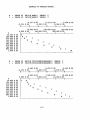
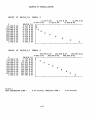
Here follows an example of a circuit-description in Panacea input-language.
The output that results from this particular example can be found in
appendix A.
title: This is an example of a Panacea circuit description.
numform: engineering, fix, digits=4
circui t ;
j1 (0,1) sinewave(2.0,0)
j2 (0,1) 2 * par;
r1 (1,0) 0.5 ;
ec1 (0,2) i(r1)*i(r1)
c1 (2,4) 22u
r2 (3,2) 0.5
r3 (3,4) 0.5
r name (3,0) i = exp(vn(4» ;
r-thisisaverylongname (4,0) 0.5
c2 (3,0) 47u ;
end;
ac;
f= an( 10, 1000, 9 )
par = 1, 2 ;
print: v(r*)
mplot: v(r name), v(r thisisaverylongname)
(options: grid, plotchar=(R,I) , width = 70, iscale)
prplot: v(r 3) (options: plotchar=@);
file: vn, C;
end;
run: ac ;
finish ;
3-4
INTRODUCTION TO PANACEA.
3.2.3
Stand Alone Statements.
In the Panacea input language the circuit and analysis descriptions are
organized in BLOCKS, like the CIRCUIT block.
However, there are also some statements that appear outside a block. In our
context the following functions are important:
LENGTH:
this function is used to specify the pagelength: after the given
number of lines a formfeed is forced, and a pageheader will be
generated. Vhen no paging is wanted, the page-length should be
set to O.
VIDTH:
This function is used to specify the width of a line of output:
for instance 80 on a terminal, or 132 on a big lineprinter.
Any output -tables or -plots will fit within the given width.
LIST/NOLIST: with these commands the echoing of the Panacea input can be
allowed and suppressed: this is very useful, for instance when a
PROCESS-block is being used of 100 pages of Panacea input, and
which is of no importance at all for the user.
NODELIST:
Vith this function, the user can indicate that he wants to get a
list of all the nodes in his circuit, with for every node a list
of the elements connected to it.
TITLE:
This title will be printed on top of every page of Panacea output.
NUHFORH:
Using this function the user can specify in what manner he wants
the values in the output to be formatted:
EXAMPLE:
- SCIENTIFIC
normal exponential notation
1.27345 E-04
- ENGINEERING NOTATION
exponential notation with the exponent
127.34500 E-06
always a multiple of 3.
- SCALED
using scaling factors like K,HL,U etc.
127.34500 U
- FIXED / FLOAT
keep the point at a fixed position,
or let it float through the number:
127.34500 E-06
127.345 E-06
98.7654 E-09
- DIGITS = k
set the precision with which the values must be printed to k.
In case of FLOAT exactly k digits are printed; in case of
FIX the number of digits after the point is always k-1;
this means that sometimes extra digits will be printed,
namely when more then one digit stands in front of the point.
R~:
Perform the given analysis, using the last analysis-block of the
given type.
FINISH:
End of Panacea input.
3-5
INTRODUCTION TO PANACEA.
3.2.4
The Circuit Block.
The CIRCUIT block contains the description of the circuit that has to be
analysed. The circuit is described by specifying every element in it: each
element is specified by a list of the nodes it is connected to, and a list of
values that specify the values of internal parameters of the element:
elemname ( nodel, node2, ..• ) parvaluel, parvalue2,
.... .,
The name of an element consists of two parts: a type indication, and an
occurrence indicator. The type-indication describes what sort of element we
have, while the occurrence indicator is used to give each occurrence of some
sort of element a unique name.
An element can be a build-in component, or a model occurrence (this can be
user defined models, or models from one of the Panacea libraries).
The build-in components.
basic elements:
R
resistor
capacitance
C
inductor
L
H
mutual inductors
E
voltage source
current source
J
controlled sources
EC I JC
EN I IN
noise sources
short circuit
S
basic devices:
diode
NPN I PNP transistor
NPN transistor with substrate
lateral PNP transistor
NIP-channel MOS
two-port described by
y I s parameters
YNPORTI
N-port described by
SNPORT
y I s parameters
The occurrence-indicator consists of one or more characters. If the first
character of it is not a digit, it must be preceded by an underscore.
Some examples of element names are:
Rl
C abc
H76d
TNS aal2b
The order in which the node-names appear in the node-list specifies which
node is connected to which terminal of the element; the names of the nodes
can be any character-string. Vhen two elements have a common node-name in
their node-lists, then the corresponding terminals are connected to each
other.
The parameter-values specify the values that will be given to certain
parameters in this element; one can specify just a list of values, which then
will be assigned to the first (n of values) parameters; or, one can specify
the name of a specific parameter-that has to be assigned.
The 'values' are specified using expressions, with as operands:
- constants,
- electrical variables (i.e. certain electrical quantities in ~he circuit),
- independent parameters.
Also, it is possible to use a TYPE SPECIFICATION. A type is a sort of
abbreviation for a list of parameter-assignments: by using a type, one does
not have to enter the complete list of parameters every time one uses an
element with some specific set of parameter-values.
3-6
INTRODUCTION TO PANACEA.
FOR EXAMPLE:
TN, has as connections: 1) collector, 2) base and 3) emitter.
The string "'Bc14SC'" is a type-specifier: the TN that is used will
get the parameter-values as specified in the definition of this type.
Then, the BETA is assigned again, overriding the assignment of this
parameter done by the type-specification.
It is assigned the result of evaluating the expression 100 * par, where
par is an independent parameter that will move through a series of
values while the analysis is being performed (see ANALYSIS block): every
time that par changes, the parameter BETA in TN_11 will also be changed.
MODELS.
Just like a program is split up in functions, a circuit-description can be
split up in sub-circuits by using models: which is very usefull when some
subcircuits appears often, and also of course for deviding a large circuit in
clearly separated sub-circuits:
MODEL: subcircuitname (terminal list) formal_parameter_list
Circuit Description
END;
Actual values will be assigned to the formal parameters
which this model is used: in every model-occurrence the
determine the setting of element-values etc. within the
is missing in the model-occurrence, it will get the for
specified default value.
by the circuit in
specified values
model. If a parameter
this parameter
The terminal list is a list in which are listed all the nodes in the model
that are connected to the outside-world. Vhen the model is used within
another circuit, these nodes will be connected to nodes in the surrounding
circuit.
The scope of names of elements and nodes is limited to the block where they
are used in: this means that inside a model we can use some name, which can
be the same as a name outside this model, without indicating the same object.
Models are used to describe a circuit in a hierarchical way, because within
a model we can use sub_models, containing sub-sub-models, etc. For example:
Model: block (a,b,c,d)
R 1 (a,b) 2
R-2 (b,c) 2
R-3 (c,d) 2
R-4 (d,a) 2
End-;
R5
R-6
R-7
R-S
(a,l)
(b,l)
(c,l)
(d,l)
Model: bigger_block (a,b,c,d) ;
block3 (5,2,c,3)
block1 (a,1,5,4) ;
block4 (4,5,3,d)
block2 (1,b,2,5) ;
End ;
3-7
/*
S resistors.
*/
/*
32 resistors.
*/
2
2
2
2
INTRODUCTION TO PANACEA.
3.2.5
The Analysis Block.
In this block the analysis to be performed is described, together with the
output that is requested for this analysis. Vhen more then one analysis must
be performed, they will be handled in separate analysis blocks.
The NAME of the block specifies the type of analysis:
DC
AC
TR
DC STAT
ACSTAT
TRSTAT
for dc analysis
for linear ac analysis
for transient analysis
dc statistical analysis
ac statistical analysis
transient statistical analysis
Vithin the analysisblock the INDEPENDENT PARAMETERS are being specified.
These are used when it is required to vary some element in the circuit during
the analysis, for example to measure the effects that result from changing
the value of some resistor. In such case, an independent parameter is used
that will step through a specified series of values; for each value, a
complete analysis will be performed.
Vhen more then 1 independent parameter is specified, then for all the valuecombinations of their series an analysis will be performed: the combinations
are generated in a lexicographically ordered way, Le. the "fastest"
independent parameter will move through its series of values, while the other
independent parameters are kept frozen; then, the second fastest indep par
will step to its next value, after which the fastest will again move through
its complete series, etc, until the second fastest par has reached its last
value: then the third steps to its next, etc, etc, until all combinations
have been processed.
The fastest changing independent parameter is called the PRINCIPAL
independent parameter; the others are called the SUBSIDIARY indep pars.
In the analysis, a STEP will be made for every value of the principal
indep par; the analysis-RUN (i.e. run over all steps) will be repeated for
all subs indep par combinations.
For an example see Appendix A; there is F the princ indep par, and par is
the subs indep par: first all output is produced with par. 1, and then
the output for par = 2.
The number of combinations of the independent parameters can be restricted
using the TRACK statement:
with this statement one can specify that some indep pars will change their
values together: when we would specify that a and b are tracked, we would get
the combinations
1,5 2,10 and 2,15. Vhen an indep par reaches its last
value, this value is repeated until the indep par with the most
values is finished.
In a TRACK statement it is also possible to use the principal indep par: this
results in a situation where we have more then 1 principal independent
parameter.
3-8
INTRODUCTION TO PANACEA.
The specification of the values for an independent parameter can be done
using special series-functions:
AN
AS
GN
GS
EN
(
(
(
(
(
x,
x,
x,
x,
x,
y,
y,
y,
y,
y,
k
z
z
z
)
)
)
)
k )
Arithmetic progression from x to y in k intervals.
Arithmetic progression from x to y, stepsize = z
Geometric progression from x to y, in k intervals.
Geometric progression from x to y, stepsize = z
Rounded geometric progression from x to y;
k = nr of intervals in a decade ( k=12 ==> E12 seriesl )
It is also possible to give a list of values; this can even be mixed with the
series functions. There is no need whatsoever for any ordering in the value
list, and values may even appear more then once.
For example:
F = AN(10,100K,30) , 200K , 300K , GN(l,1000,17), 134.5567 ;
Output will be generated for every F-value, in the precise order in which the
values were given; if it's plotted you'll probably get a real weird plot,
but .. it's what was requested by the user.
Besides the independent parameter specifications, in the analysis block we
find the OUTPUT SPECIFICATIONS: these commands specify the output that must
be created for this analysis.
For a description, see the next section.
3-9
INTRODUCTION TO PANACEA.
3.2.6
THE PANACEA OUTPUT SPECIFICATIONS
The Panacea output is specified using special outputcommands that have the
following format:
outputcommand: output_item-list
3.2.6.1
(OPTIONS: options-list);
The Output Commands.
PRINT
PLOT
PRPLOT
MPLOT
FILE
HISTOGRAM
creates tabular output.
creates plots of the given items; one item per plot.
creates plots of the given items, thereby also printing on each
line the value of the item; one item per plot.
creates plots of the given items; more then one item per plot:
the number of items is determined by the number of plotchars.
(A plotchar is a character that is used to produce a plot with.)
creates file-output: makes a file in the SDIF format, containing
the analysis-results for the requested items.
This file can then be used as input for certain post-processors,
for instance to create a real plot, in stead of the Panacea
line-printer plots.
creates histogram-output in case of statistical analysis: in the
resulting plot, the statistical distribution is visualized.
Yith respect to the PLOT, MPLOT, PRPLOT and HISTOGRAM outputcommands, an
important side-effect should be noted:
In order to create the correct SCALING of the y-axis, we must know BEFORE we
start printing, what the MINIMUM and MAXIMUM values of the item to be plotted
are. This demands that we first must STORE ALL THE RESULTVALUES of the item,
and then determine the minimum and maximum values, which then determine the
scaling of the y-axis; finally, the plot can be made.
This is the major reason for the Output Processor to be designed as a
POST-PROCESS: FIRST collect all the data necessary for the output, THEN
format the requested tables, plots etc.
Processing the output as a post-process has the drawback that for a big
simulation-job in an interactive environment, the user has to wait a long
time before seeing any output, at whch moment he gets everything at once.
Therefore, Panacea will probably get an extra output-command, the
MONITOR: command: this command will write analysis-results to output as soon
as they are produced, i.e. after every analysis-step the values of the
requested items are written to output.
The items that can be used in a MONITOR command are restricted to LEVEL 1
items (See next section): this because an higher-level item can only be
produced in a post-process.
3-10
INTRODUCTION TO PANACEA.
3.2.6.2
The Output Items.
The items that can be requested are all kinds of electrical quantities and
other results that follow from the analysis, see table below.
When a node or element specification is part of the item, wildcards are
allowed: for instance, It PRINT: VN, V(R*); It. In the table must appear:
- VN
all the nodal voltages of the circuit.
- V(R*) the voltages across every resistor in the circuit.
Output items:
1)
2)
3)
4)
5)
6)
7)
8)
9)
10)
11)
12)
13)
basic element values.
parameter values.
expressions (output-functions may be special operands).
nodal voltages (with respect to ground).
voltages between any two nodes.
electrical variables.
voltages across an element.
terminal-currents for an element.
power-dissipation in an element.
electrical state: voltage across, current through and power
dissipation in an element.
Output-functions: see below.
Sensitivity and Gradient:
Sensitivity and rate of change of an output-quantity (e.g.
electrical variable or a nodal-voltage) with respect to the value
of a particular circuit element or parameter.
For AC and ACSTAT analysis a great number of extra output-facilities
are available:
Twoport outputs:
All sorts of Twoport outputfunctions, using twoport-quantities like
the input reflection coefficient.
Noise outputs:
In noise analysis:for example, NOISEMSVDENS: noise power density.
Statistical outputs:
In statistical analysis: NOM, MEAN, SPREAD, LIMITS.
An electrical variable is a certain electrical quantity in the circuit, that
has been given a name of its own. The usage of electrical variables was
necessary in Philpac, in order to describe the relation between certain
quantities: for example,
i1 (r1) ;
i1
electro variable, gIvIng the current through r1
ec1(0,2) i1 * i1;
ec1 = controlled source, value = i(r1) * i(r1).
In Panacea, the use of electrical variables is not necessary anymore: it is
now possible to directly use the i(r1) in the specification of the source:
ec1(0,2) i(r1) * i(r1);
But in order to maintain the compatibility between Philpac and Panacea, the
use of electrical parameters is also implemented in Panacea.
3-11
INTRODUCTION TO PANACEA.
3.2.6.3
The Output Functions.
It is possible to specify in Panacea that one is not interested in the value
of some circuit-quantity for every analysis-step made, but that one instead
is interested in some result-value that is computed using the result-values
for every analysis-step: for example, the mean of the current through some
element. For a list of the possible output-functions, see the table below.
It would be nice, if we could use the results of these output-functions as
operands in an output-item expression, so that we for instance could request:
PRINT: V(R1) - MEAN ( I(R2) );
Vhen we consider this expression, it is clear that first the result-value of
the output-function must be known, before we can print the table containing
for every value of the principal independent parameter the value of
V(R1) - MEAN ( I(R2) ).
This can be expanded to more complex situations, like:
MAX ( I(C3) - VALUE( MIN( V(R1) - MEAN(I(R2) - VALUE(HAX(par_A»
»
»
Ve now get LEVELS in our output-items: first the results on the lowest level
must be known, before we can compute the values at the second level
(i.e. the MAX must be known before I(R2) - VALUE (MAX(» can be determined).
Then we can handle the next level ( i.e. MIN(V(R1» - MEAN (i-VALUE() ) ),
etc, until all levels have been determined, after which the results can be
written to output.
The algorithm to handle these output-expression levels requires that when
computing the results for the next level, we must have access to the
analysis-results; this can be done by analysing the circuit again, which of
course is very inefficient, or by storing all the analysis-results that are
necessary for the computation of the expression, in such a way, that we can
retrieve them every time again when we handle the next level.
Because the output was already planned as a post-process (see the remark at
the paragraph over the Output-commands) the last solution will be not to
difficult to implement, being only an extension to the storage-process.
BASIC OUTPUT FUNCTIONS
FALL
MAX
MEAN
MIN
RISE
SUM
VALUE
p.i.p.v. for which the item passes with a negative slope through O~ ,
p.i.p.v. where the item reaches its maximum.
mean value of the given item,over every value of the princ indep par.
p.i.p.v. where the item reaches its minimum.
p.i.p.v. for which the item passes with a positive slope through O.
The INTEGRAL of the given item over all values of the princ indep par.
The VALUE of the item for the given p.i.p.v.
(p.i.p.v.
principal independent parameter value.)
3-12
INTRODUCTION TO PANACEA.
3.2.6.4
The Output Options.
The following options can be specified for the command mentioned:
PRINT:
WIDTH
RANGE
XVAR
XRANGE
set the line-width to the given value, for this command only.
limit the princ indep par values to the given range.
use another parameter than the princ indep par for the x-axis.
When using XVAR, limit the values of this par to the given range
PLOT, PRPLOT:
WIDTH
GRID
PLOTCHAR
RANGE
XVAR
XRANGE
YRANGE
XLABEL
YLABEL
set the line-width to the given value, for this command only.
superimpose a rectangular grid upon the line-printer plot.
set the plotchar that is used in the plot to the specified char.
limit the princ indep par values to the given range.
use another parameter than the princ indep par for the x-axis.
When using XVAR, limit the values of this par to the given range
the y-axis will be scaled using the specified range.
the x-axis is labelled with the specified string.
the y-axis is labelled with the specified string.
MPLOT:
The PLOT options, but now more then a single plotchar and YLABEL may be
specified, because now more then one item can be plotted at the same time.
ISCALE
individual scales are chosen for every item to be plotted.
FILE:
RANGE
XVAR
XRANGE
limit the princ indep par values to the given range.
use another parameter than the princ indep par for the x-axis.
When using XVAR, limit the values of this par to the given range
HISTOGRAM:
WIDTH
RANGE
XVAR
XRANGE
YRANGE
XLABEL
YLABEL
INT
set the line-width to the given value, for this command only.
limit the princ indep par values to the given range.
use another parameter than the princ indep par for the x-axis.
When using XVAR, limit the values of this par to the given range
the y-axis will be scaled using the specified range.
the x-axis is labelled with the specified string.
the y-axis is labelled with the specified string.
the number of histogram-intervals on the x-axis.
3-13
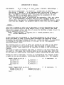
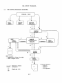
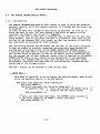
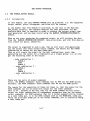
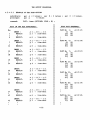
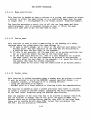
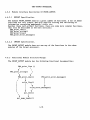
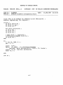
THE OUTPUT PROCESSOR.
4.1
THE OUTPUT-PROCESSOR STRUCTURE.
,I
PANACEA MAIN
I
1
,-
I
I
I
I
2
Y
I
I
Y
EXPAND
INPUT
READ
INPUT
I
I
I
3
Y
PERFORM
ANALYSIS
I
I
4 I
.II:
1&
.II:
Y Y
\
I
I
I
I
I
I
I
I
I
8 I
y
CONTROL
OUTPUT
I
I
5 I
\
I
I
I
I
I
I
I
I
I
.II:
.II:
.II:
Y y
I
I
1
....
7
I
\
.
SDH
-INPUT
-OUTPUT
1/
1/
II
n
\
I
I
I
I
I
I
I
I
I
I
I
,
_ _ _ _ _ _ _ _ _1
.II:
I
.II:
111
Y
1&
.II:
.II:.!!:.II:.II:.!!:.II:.!!:.II:.II:.II:.II:.II:.!!:.!!:.II:.II:.II:I
\
.-,----.;;..;~~-
I
\
FORMAT
OUTPUT
---------:.-13:::---"\I
14
SDH-Files:
- Temporary files for HIR
- SDIF output-file
I
.II:
I
.II:
I
.II:
Y y
PRINT
OUTPUT
15
----->
.!!:.!!:.II:.!!:.II:>
II
1/
n
II
II
n
I
I
I
I
\ ..
I
I_I
Function Calls
Dataflow.
Physical I/O
4-2
Printed Output:
- Tables, .
- Plots,
- Histograms.
I
THE OUTPUT PROCESSOR.
4.1.1
Explanation.
When Panacea is activated, it starts reading the input-file containing the
circuit-description (1). This input will then be expanded (2) in such a way,
that afterwards the analysis can be performed on the resulting analysisdatastructures. Then, the analysis is done. (3)
The analysis of a circuit consists of separate analysis-steps: for every
combination of the subsidiary independent parameters, a complete analysis of
the circuit will be performed. Such an analysis consists of a series of steps
over the principal independent parameters.
After a step has been analysed, the analysis datastructures contain the
simulationresults for this step: from these structures we now must extract
the values that belong to the in the output commands requested items.
This is done by calling from the Analysis module certain functions in the
module CONTROL OUTPUT. (4) These functions will gather the required data.
The output is organised in such a way, that we will first perform the
complete analysis, before we start producing any of the requested output; we
will SAVE the analysis-results temporarily, using functions in the
HANDLE INTERMEDIATE RESULTS module. (5)
This module (abbreviated to HIR) tries to store the data in core; however,
when there is too much data, it will open a file and write the data into it;
this file has the standard SDIF format, and is written using the functions in
the SDIF_IO module. (6) (7)
After the complete analysis has been finished, we shall start producing the
requested output. (8)
First, we will compute all the higher level output-items, i.e. expressions
using both analysis-results and output-function results.
This is done by the LEVEL HANDLER (9) which can be found in the function
OUT terminate output() in-module CONTROL OUTPUT.
It retrieves the data that was stored in-the HIR module, processes it and
then writes the new results back to the HIR module. This will be repeated
until all the levels have been processed. (10)
Then the FORMAT OUTPUT module is activated (11) which retrieves the data
from HIR (12) and uses it to produce the output that belongs to the given
output commands.
FILE output will be created using the functions in the SDIF 10 module (13).
The other outputcommands result in printed output; after a line of output has
been created, it will be handed over to the PRINT OUTPUT module (14).
This module takes care of the layout of the Panacea-output (creating a pageheader on top of a new page, and handling line-overflow in a decent way: the
last word is wrapped around to the next line). It is an extra layer between
Panacea and the outside world, EVERYTHING that is printed during a Panacea
job goes via this module: be it input-listing, error-messages, or lines of
output -tables or -plots.
4-3
THE OUTPUT PROCESSOR.
4.2
LIST/CLASSIFICATION OF USED SYMBOLS/NAMES.
HIR
HANDLE INTERMEDIATE RESULTS.
This module is used to store the analysis results, until they can be
processed in the output processor.
There are functions for storing data, for retrieving data, and for
initializing, rewinding and terminating the used file.
SIO
SDIF INPUT/OUTPUT.
This module handles the file-io with files in the standard SDIF
fileformat, consisting of INFO and TITLE records, followed by
HEADER records with the names belonging to all values occurring in
the TUPLE records that follow hereafter.
PRO
PRINT OUTPUT.
This module is used as an extra interface between Panacea, and the
paper-output: we check on line-overflow and on page-overflow.
The module is also used for printing error-messages.
FTO
FORMAT OUTPUT.
In this module the Panacea output is formatted: plots and tables are
created, and file-output is produced.
INDEP array,
RESULT array,
OUTFUNC array
This are the names of the arrays that are used while evaluating all
output-expressions, to store the resulting values.
The INDEP array is used to store the current subsidiary independent
parameter values, the RESULT array to store the principal indep par
values and the values of every analysis-step dependent output item,
and the OUTFUNC array is used to store the values belonging to
output-functions.
4-4
THE OUTPUT PROCESSOR.
4.3
THE CONTROL OUTPUT MODULE.
4.3.1
Introduction.
This module controls the output process. It contains functions that:
- expand the commands that are read from input;
- collect independent parameter values and analysis results;
- terminate the output process, by evaluating all the higher level items, and
then producing the requested output (by calling FTO_format_output(».
4.3.2
4.3.2.1
The
-
Module Interface Description Of CONTROL OUTPUT.
EXPORT Specification.
module CONTROL OUTPUT exports a lot of functions:
for storing and retrieving of information concerning the NUMFORH-format;
for storing and retrieving of information concerning the TITLE string;
for creating the NODELIST output.
for giving the pointers to the data-structures in CONTROL OUTPUT that
contain all the information with respect to the output to-be produced.
The most important of these structures is the OUT general data
data-structure, see below.
--
The most important functions (these will be described in the next sections)
are:
OUT expand output()
OUT-subs indep par values()
OUT-results() OUT-function results()
OUT=terminate_output()
The OUT GENERAL DATA data-structure:
This structure contains all the necessary information about the output
process: it contains general information like the time and date of the
current Panacea-job, and pointers to the lists of output item - descriptions:
this are structures that contain the name of an item, and a pointer to the
location where we can find the value that belongs to this item. This location
is fixed, and is located within the INDEP-, RESULT- or OUTFUNC- array.
When producing output, these arrays are filled by calling the HIR retrievefunctions, with the results that belong to a certain step made in the
Analysis, and we will use the value on the location where the itemdescription points to. After having processed the current step, we move to
the next step in the Analysis: we will re-fill the arrays, and we can now
produce the next line of output by using the new value that has appeared on
the given location.
4-5
THE OUTPUT PROCESSOR.
4.3.2.2
IMPORT Specification.
The CONTROL OUTPUT module uses a number of functions from the other modules
in the Output Processor:
HANDLE INTERMEDIATE RESULTS:
This module is used to store all the analysis results, that later will
be used to generate the output with:
HIR initialize ()
HIR-store INDEP ()
HIR=store=RESULT ()
HIR store OUTFUNC ()
HIR-retrieve INDEP ()
HIR-retrieve-RESULT ()
HIR-retrieve-OUTFUNC ()
HIR=terminate ()
FORMAT OUTPUT:
FTO format_output()
Initializes the HIR module.
stores a set of subs indep par values.
stores the array of analysis-results for
the current prine indep par value.
stores a set of output-function values.
retrieves a set of subs indep par values.
retrieves a set of analysis results.
retrieves a set of output function results.
terminates the storing of-data into the
HIR datastructures.
Creates the output that belongs to the set
of commands that has been read from input.
4-6
THE OUTPUT PROCESSOR.
4.3.3
Function Descriptions.
This function is used to expand the list of commands that are read from input
thus creating data-structures that can be processed by the output-processor
for creating output.
The most important action is the creation of the link between the requested
items, and the analysis data-structures: when some item is read, we still
don't know where the value of this item is to be found.
The details of this expansion are omitted, because of the fact that for
understanding them one has to know the analysis data-structures in precise
detailj which was the reason that the expand has been implemented by my
coach, him being the one who developed these datastructures.
Besides creating the link to the analysis, other expansions must be done:
- every VILDCARD that is found in an item must be expanded into a list of
occurrenceSj
- whenever higher-level output-items are found, being expressions that use
output-functions as operands, these items must be expanded into:
- a set of lower-level subexpressionsj
- an expression, that uses as operands references to the results of these
lower-level subexpressions.
The sub-expressions will be treated in the same way, resulting in a tree
of expressions, with as leaves only LEVEL 1 expressions: this are
- references to direct analysis-results,
- constants, or
- output-functions using only LEVEL 1 parameters, like MEAN ( V(R2) ):
such an output-function can be evaluated on the fly while performing
the analysis, each time updating the stored value.
In the function OUT results() we now will save all the LEVEL 1 results.
After the complete analysis has been finished, for every subs indep par
combination, the function OUT terminate output() will be called, where we
will evaluate all the higher level expressions: before an expression on a
certain level is evaluated, the values of all its lower level operands
must have been determined.
4-7
THE OUTPUT PROCESSOR.
This function stores a set of values for the subsidiary independent
parameters.
In this function, first an array containing the current values for the subs
indep pars is fetched, using a function in the Panacea-module that handles
the independent parameters.
Then this array is stored, by calling the function HIR_store_INDEP().
4.3.3.3
OUT results.
After an analysis step has been performed, the analysis-results must be
extracted from the analysis data-structures. These results, together with the
current values of the prine indep pars, then are stored in the HIR
data-structures.
First, the function will get the current prine indep par values, in the same
way as the subs indep par values were handled.
Then, a function is called that will evaluate all the LEVEL 1 output-items:
using the link between an item and the analysis-datastructures, we will
collect the current value of the item. Vhen an item is an expression that
uses as operands analysis-results, all the operand-values will be fetched,
and the expression will be evaluated.
Vhen the item is a LEVEL 1 output-function, we will update the value that was
stored for it, using the new values of the operands for this function:
for example, when MAX ( I(Cl) ) is demanded, we must check if the current
value of I(Cl) is bigger then the value that is stored for the MAX-function;
if so, the MAX-function will be set to this new maximum.
4.3.3.4
OUT function results.
This function handles the results of the LEVEL 1 output-function items:
after a complete analysis-run over the prine indep par has been completed,
the result of the item has got its final value, and can now be saved in the
HIR data-structures, using the function HIR_store_OUTFUNC().
4-8
THE OUTPUT PROCESSOR.
Vithin this function, we will
- handle all the higher level output-items;
- create the output, by calling the FTO format_output() function.
The LEVEL HANDLER.
The evaluation of the higher level items is performed level by level,
starting at Level 2 (the Levell results were already evaluated during the
analysis). After having all the items at Level 2, we have determined the
values of every operand of the Level 3 items, so then we can compute these;
and so on, until all the items have been evaluated.
The algorithmic structure of the Level-Handler is as follows:
FOR( every level other then Levell) {
HIR_rewind();
1* start reading the in the HIR module stored data *1
FOR ( every combination of subs indep par values ) {
HIR retrieve INDEP();
HIR-store INDEP();
HIR-retrieve OUTFUNC();
FOR-( every step made over the prine indep par in the analysis ) {
HIR retrieve RESULT();
Evaluate the-items on the current Level;
HIR_store_RESULT();
}
HIR_store_OUTFUNC();
}
}
The first FOR-loop causes every level to be handled, every time restarting
retrieving data from the beginning.
Then we will for every value-combination of the subs indep pars, evaluate the
items on the current level for every step made over the principal indep par:
via HIR retrieve INDEP() we fetch the next indep-par combination, and then
store this combination back to HIR via HIR store INDEP().
Next, we retrieve the OUTFUNC-resultvalues-as stored for the current subs
indep par combination, via HIR retrieve OUTFUNC().
Then, for every step made over-the principal independent parameters, we use
the already produced lower level results for this step (this includes the
lower level OUTFUNC results) as operands while computing the values of the
now to be evaluated items.
This is done by retrieving the data that has been stored in the HIR module,
using the function HIR retrieve RESULT() , and then add to this array of
results, the results of the evaluation of the items on the current level.
The new result-array then is saved, using the HIR_store_RESULT() function.
After having repeated this for every step, we have reached the point where
the output-function items in the new level have got their final values, and
therefore these values can be saved, using the HIR_store_OUTFUNC() function.
4-9
THE OUTPUT PROCESSOR.
4.4
THE HANDLE INTERM RESULTS MODULE.
4.4.1
Introduction.
The HANDLE INTERMEDIATE RESULTS (HIR) module is used to store the produced
analysis results, until-the complete analysis is finished and the output can
be produced.
In order to make this storage as efficiently as possible, we will try to
store the data in core. For this purpose a big block of memory will be
reserved: the default size is set to 1 Megabyte.
Yhen it occurs that so much data is produced that it does not fit into this
block anymore, then we will write the data to a diskfile: this file will be
written in the standard SDlF file format, so that the contents of this file
may eventually be processed by other programs.
The interfacing between the HIR module and the rest of the output processor
is kept as simple as possible: separated functions have been created for
storing and retrieving of data in the lNDEP, RESULT and OUTFUNC arrays.
A function has been made to position the "datapointer" to the beginning of
the current block of results, so that we can easily restart retrieving data
for the current set of subs indep par values (this is required in the module
FORMAT OUTPUT where we must reposition the datapointer to the beginning
of a block, for example when we start with the plot for some next item).
Furthermore, functions have been made for initialization, termination and
restarting of the storage process.
The HIR - module can be operated in some various ways:
- VRITE ONLY:
This mode of operation is active during the analysis-phase, when we will
write the analysis-results to the HIR module:
FOR every subs indep par value-combination:
HIR store INDEP();
FOR-every-step made over the princ indep pars: {
do analysis step; /* after this action, the RESULT array
/* contains the new result-values.
HIR_store_RESULT ();
}
/* after all steps have been made, the OUTFUNC array contains */
/* the final values of the LEVEL 1 output functions.
*1
HIR_store_OUTFUNC ();
}
4-10
*/
*/
THE OUTPUT PROCESSOR.
- READ/WRITE:
This mode of operation is active when the LEVEL HANDLER is computing all
the results for the output-items of Level 2 and-higher:
The results that were stored in HIR are retrieved, and the results for
the next level will be computed using these results. The resulting
array, updated with the new values, is then stored again via HIR, so
that on the next level we can use the just computed results. See the
section that describes the LEVEL_HANDLER for the algorithmic structure.
- READ ONLY
Vhen we enter the FORHAT OUTPUT proces, we will retrieve the stored
results and use them to create our output -tables and -plots.
FOR every subs indep par combination: (
HIR retrieve INDEP();
FOR- all commands: (
FOR all output-figures for this command
/* i.e. all separated plots etc. */
HIR reposition on INDEP()
HIR-retrieve OUTFUNC();
create the table/plot, by retrieving every RESULT array;
}
}
}
Ve thus get blocks of output, one block for every indep par combination, each
containing all the output tables and plots that belong to this combination.
Host of the given commands, result in more then 1 table/plot: for instance a
PLOT command with 6 items will result in 6 plots, each of a single item.
For producing these plots, we must restart retrieving the RESULT-data for the
current subs indep par combination for every next plot: this is done by the
call to HIR reposition on INDEP(). Then the plot is made, by retrieving the
RESULT-data-for every princ indep par value, and using this data while
creating the plot.
4-11
THE OUTPUT PROCESSOR.
4.4.2
Module Interface Description Of HANDLE INTERM RESULTS.
4.4.2.1
EXPORT Specification.
The module HANDLE INTERMEDIATE RESULTS exports the following functions:
HIR initialize ()
HIR-terminate ()
HIR-store INDEP ()
HIR-store-RESULT ()
HIR-store-OUTFUNC ()
HIR=reposItion_on_INDEP ()
4.4.2.2
HIR rewind ()
HIR-reopen ()
HIR-retrieve INDEP ()
HIR-retrieve-RESULT ()
HIR-retrieve=OUTFUNC ()
IMPORT Specification.
The HIR module uses the functions in the SDIF 10 module, in order to be
able to write/read the file that contains the-intermediate results, in those
cases where there is very much data.
4.4.3
Functional Module Structure Design.
The 'store' -functions make use of the HIR write file() function:
whenever it is detected that we have not enough space left to store the array
of values, the contents of the memoryblock is saved to the file. This file
can therefore be seen as consisting of blocks of data: each block consisting
of the contents of the coreblock at that time.
The 'retrieve' -functions make use of the HIR read file() function:
when a file is being used, and we detect that we have reached the end of the
data stored in the coreblock, then we will have to read data from the
disk-file: the next block will be read.
All the functions in the HIR-module are heavily related to each other via the
global static datastructures in the HIR-module: there are numerous boolean
variables that are used for stering the store/retrieve-process, each of which
can be set in some function and then later will influence the programm-flow
in some other function.
4-12
THE OUTPUT PROCESSOR.
4.4.4
4.4.4.1
Function Descriptions.
The Used Data-structure:
Within the HIR module a linked list of structures is used, each element
repesenting a certain subs indep par combination: the elements describe the
places where the data that belongs to this combination can be found:
- there is a pointer to an array that contains the subs indep par values;
- there is a pointer to the place in the coreblock where the first
RESULT-array contents is stored;
- there is a pointer to an array that contains the OUTFUNC array contents.
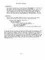
Besides this list, another important structure is used: a big block of memory
in wich the RESULT-data will be stored. It is nothing motre then a big array
of reals, with a default size of 1 Megabyte ( == 128k reals).
HIR linked-list
"
Coreblock
yy
:I
p_INDEP_array
===>
p_First_RESULT
===========================>
p_OUTFUNC_array
===>
:I
INDEP values [
OUTFUNC values [
p next
II
yy
1r------1~
I First RESULT array I
I
I
I Second"
"
I
I
I
I
I
~I First
~
RESULT array I
of next subs comb •
With regard to the RESULT and OUTFUNC arrays, it should be noted that they
contain value-fields for the items of EVERY level: the value-fields belonging
to items on not yet evaluated levels will remain empty until the level where
they belong to is evaluated: when evaluating such a level, we will retrieve
the data from Core, by copying an array of values from the Coreblock into the
RESULT-array. Then the results of the items on this level are added to the
array, by storing the result-values in the fields dedicated to them:
hereafter the RESULT-array is written back to Core, where it will be stored
on the same location as where it originally was read from.
When so much data was produced in the analysis that a file had to be be used,
we must save the contents of the coreblock after having processed the last
RESULT-array in the current block: after this, we then read the next block of
data from the file; we process this block, save it, read the next, etc. etc.
This causes us to use 2 files, one for writing data to, and one,for reading
data from: this, because it is not possible to write data somewhere inside an
already existing file: data can only be added to the ened of a file.
When stepping to the next level, the file that WAS the write-file will become
the read-file for the new level.
4-13
THE OUTPUT PROCESSOR.
4.4.4.2
HIR store INDEP.
In this function, first a new element is added to the linked list. Then, the
values of the current subs indep par combination are stored.
4.4.4.3
HIR store RESULT.
This function is used to store the contents of the RESULT array into the
coreblock, when there is still room for it left: otherwise, we first write
the contents of the coreblock to file using HIR write to file(), and then
store the RESULT array in the now vacant coreblock. - -
4.4.4.4
HIR store OUTFUNC.
4.4.4.5
HIR retrieve INDEP.
4.4.4.6
HIR retrieve RESULT.
-
This function stores the array of output-function results. The values in this
array have their final values after all the analysis-steps have been made for
the current subs indep par combination, therefore these results will be
stored as the last array of the block of data for some subs indep par comb~
-
Steps to the next element in the linked-list, and copies the content of the
array pointed to by the p INDEP array into the INDEP array.
Initializations are made make sure that the first time that the function
HIR retrieve RESULT() is called, it will return the first RESULT-array for
this subs indep par combination.
The function returns FALSE when there is no next list-element available.
-
This function retrieves the next set of RESULT data from the coreblock and
stores it in the RESULT array; the function returns FALSE after having
reached the last stored array.
4-14
THE OUTPUT PROCESSOR.
4.4.4.7
HIR retrieve OUTFUNC.
This function retrieves the OUTFUNC array that is pointed to by the current
list-element. Here we find the reason why the content of the OUTFUNC array is
NOT stored in the coreblock, but in separate arrays:
Yhen retrieving data in the LEVEL HANDLER, we will use the results of the
lower-level items to compute the Items on the current level. This means that
the contents of the OUTFUNC array must be available for the evaluation; and
because it is possible that the amount of RESULT-data for a single subs indep
par combination is so much that it does not fit into the coreblock at once,
it is clear that we can not put the OUTFUNC behind the RESULT data in the
coreblock. Ye can not put it in front of the RESULT data neither, because
then we get into troubles when we have finished an analysis-run and we have
to store the OUTFUNC array.
Thus, the easiest solution is to store the OUTFUNC array in a separate array
that can always directly be accessed.
This function is used to reinitialize the HIR module in such manner, that we
can restart retrieving the data for the current subs indep par combination
(READ ONLY mode only).
The function steps back to the previous element in the linked list; when we
now after the call to HIR reposition on INDEP make a call to the function
HIR retrieve INDEP() we step to the element after this previous element,
i.e~ we simply re-enter the list-element of the current subs indep par
combination, and we can now restart retrieving the RESULT data for it.
4.4.4.9
HIR initialize.
This function initializes the HIR module: in it, the coreblock is allocated.
Because of the fact that a very large block is taken, it is well possible
that an allocation problem occurs, i.e. there is not enough free memory.
In such a case, we simply try to allocate a more modest block, and repeat
this procedure until the allocation succeeds, or until we find that there is
too little free memory for even a minimum-sized coreblock, in which case an
errormessage is created, and Panacea aborts.
It is possible for the Panacea-user to specify the size of the coreblock: via
a parameter in the Change-block in the Panacea-input, the coreblock-size can
be set to a smaller or bigger value.
4-15
THE OUTPUT PROCESSOR.
4.4.4.10
HIR terminate.
This function is used to stop the storage-process: all open files are closed.
4.4.4.11
HIR rewind.
This function is used in the READ/WRITE mode when switching from one level
to the next level: the current WRITE file will become the READ file of the
next level, and the current READ file will become the new WRITE file.
4.4.4.12
HIR_reopen.
This function is used in the READ ONLY mode: it opens the last used WRITE
file for read. The data in this fIle is the data that results after the last
level has been handled by the LEVEL HANDLER: this is the data that has to be
used to create the output.
-
4-16
THE OUTPUT PROCESSOR.
4.5
THE FORMAT OUTPUT MODULE.
4.5.1
Introduction.
In this module, the real PANACEA OUTPUT will be produced, i.e. the requested
output tables, plots, histograms, and files will be created.
At the moment that this module is activated, by the call to the function
FTO format output(), the complete analysis has been performed. All the
analysis-data that is required in order to produce the correct output, has
been generated, and has been stored using the HANDLE INTERMEDIATE RESULTS
module.
Yhen we now start producing the requested output, we will retrieve the data
from the HANDLE INTERMEDIATE RESULTS data-structures, and with this data we
will create our plots, tables-etc.
The output is organised in such a way, that we will start with generating
ALL the output (for every normal output command, see below) for the FIRST
combination of values for the subs indep pars.
Then we will create the output for the next combinations, every time
generating all the output for a combination as a single group: i.e. we will
get the following order in the output:
- subs combination 1 TABLE 1
PLOT TABLE 2
- subs combination 2 TABLE 1
PLOT
TABLE 2
- subs combination 3 -
There are two sorts of output commands:
First, the NORMAL commands: those commands that do NOT use the XVAR option.
Secondly, the XVAR commands: those commands that DO use the XVAR option.
The reason for the separation of these two types is, that the output for the
XVAR commands can not be mixed with output for the other commands.
This is so , because of the fact that for the XVAR command we will create
output for other combinations of independent parameters then for the normal
output commands: the XVAR parameter that for a normal command will be treated
as a subs indep par, is in the XVAR command used as the PRINCIPAL indep par,
while the principal indep par of the normal commands, now is treated as being
a subs indep par.
4-17
THE OUTPUT PROCESSOR.
4.5.2
Module Interface Description Of FORMAT OUTPUT.
4.5.2.1
EXPORT Specification.
The module FORMAT OUTPUT has only 1 function that is being exported:
FTO_format_output()
It is called from the module OUTPUT, in function OUT terminate output()
After the analysis has been completed and the LEVEL HANDLER has evaluated all
higher level items, the output can be produced.
-
4.5.2.2
IMPORT Specification.
The FORMAT OUTPUT module uses a number of functions from the other modules in
the Output-Processor:
HANDLE INTERMEDIATE RESULTS:
This module has stored all the analysis results, that now will be used
to generate the output: the data will be retrieved using the functions:
HIR reopen ()
HIR-retrieve INDEP ()
HIR-reposition on INDEP ()
HIR=retrieve_RESULT ()
HIR retrieve OUTFUNC ()
restart retrieving data from the beginning.
retrieve set of subs indep par values.
restart retrieving data for this INDEP set.
retrieve array of results for next
principal independent parameter value.
retrieve set of output-function values.
SDIF INPUT/OUTPUT:
All exported functions; used while creating FILE output, which will be
a file in the SDIF format, containing the results for the in the
FILE: - statement requested outputitems.
PRINT OUTPUT:
All exported functions: used while creating output,
Everything that is written by Panacea to (standard)
buffered by the PRINT OUTPUT module, in order to be
formfeeds and pageheaders on the right moments, and
line-overflow.
4-18
other then FILE:
Output is
able to generate
to prevent
THE OUTPUT PROCESSOR.
4.5.3
Functional Module Structure Design.
The FORMAT OUTPUT module has the following functional decomposition:
FTO format output
I
J
I
I
I
I
I
I
I
I
I
I
I
I
I
I
I
I
controls the format process.
handle options
handle-XVAR
process the options list.
gather and format data for XVAR commands.
FTO create INDEP header
print list of subs indep par names+values
uses:
create list dump
format the output for-a PRINT command.
uses:
create table
create-list dump
format the output for-a (PR)PLOT command.
uses:
create plot
create-list dump
format the output for-a MPLOT command.
uses:
create mplot
create-list dump
format the output for-a FILE command.
uses:
write block to file
HISTOGRAM output: not yet implemented.
FTO_print
FTO_plot_prplot
FTO_mplot
FTO file
FTO_histogram
create_list_dump
makes a list of outputitems and values.
create table
I name substitution
I centre name
I format=value
format a single table.
replace too long names by an alias.
centre an item-name above its column.
format a floating-point value.
create plot
create-mplot
I compute header
I print header value lines
I create interval line
I format-value -
make a plot of the given item.
make a mplot of (nr of plotchars) items.
determine the plot scaling.
prints the scale-lines of the y-axis.
make a +---+---+-- •• line.
format a floating-point value.
write block to file
write data for current INDEP set.
4-19
THE OUTPUT PROCESSOR.
4.5.4
Function Descriptions.
In the FTO format output() function the list of outputcommands is being
processed, to produce the required output tables, plots, file etc.
First, the 'normal' outputcommands are handled, creating all the output for
a certain combination of subs indep par values at once:
FOR ( all subs indep par value-combinations ) {
FOR ( all NORMAL commands ) {
handle options (command) ;
create-output belonging to the current command
}
}
Then, we create the output for the XVAR commands:
FOR ( all XVAR commands ) {
handle options (command)
handle=XVAR (command) ;
}
The handle XVAR() function shall create the output for the given command, for
every combInation of the not-XVAR indep pars.
The FILE command is treated as a normal outputcommand. Not because the output
should be grouped for a certain set of subs indep par values, as for the
normal printing output commands, but only for efficiency reasons:
we now can use the data that was read for the other normal outputcommands,
to produce a block of data in the file-output, containing all the analysis
results belonging to the current subs indep set.
In case we are working with large amounts of data, so big that in the HIR
module data is written to a temporary disk-file, we now save ourselves
a scan through this file, which would be necessary when we would treat the
FILE command separated from the normal output commands.
4-20
THE OUTPUT PROCESSOR.
4.5.4.2
Handle XVAR.
In the handle XVAR() function the data for
from the HANDLE INTERMEDIATE RESULTS module,
that contains a-set of outputitem values for
parameter that is being used.
Then this datastructure is used to generated
the given command.
the given command is collected
resulting in a datastructure
every value of the XVAR
the output table or plot for
This process will repeat it self for every combination of values for
subsidiary AND principal independent parameters, but EXCLUSIVE the XVAR
parameter.
As a result, we must very often scan through the analysis data stored by
the HIR module: and in case that we have so much data that a file is
being used to store the data in, this means that very much file-access
is necessary: which takes a lot of CPU-time.
An exception to this occurs when the XVAR is just another PRINCIPAL
independent parameter: in that case we only have to swap the XVAR and the
most principal independent parameter and then produce the tables, because
the values of ALL the prine indep pars are stored in the RESULT arrays.
Ve use a datastructure to store the retrieved results in, to limit the
number of file scans to a minimum: for example, when a PLOT: command is given
with 10 outputitems, this results in 10 separated plots. Vhen we now would
create the plots by scanning through the file, every time retrieving only the
value for the current outputitem, we would make 10 file-scans; when we first
collect the data and then produce the plots using the data that was stored
in the datastructure, we need only a single file-scan: i.e. we trade speed
for memory-usage.
A second reason for using the datastructure is that we must compute the
maximum and minimum values of the items to be plotted, these values are
required for the scaling of the y-axis of the plot.
For normal PLOT commands we can determine the max and min of the items while
evaluating the items themselves; for a XVAR plot, it's NOT possible to do so:
we will have to compute the min and max just before we start the plot.
To minimize file-access we now use the data-structure in which all the
XVAR-data is stored; thus we can compute the max and min without having to
scan the file.
4-21
THE OUTPUT PROCESSOR.
4.5.4.2.1
EXAMPLE OF THE XVAR-OPTION:
subsidiary:
principal:
command:
37
INDEP:
RESULT:
42
RESULT:
43
INDEP:
RESULT:
par
par
A: 2 values; par
p
6 values
PLOT: items (OPTIONS: XVAR
B: 3 values
par
C
2 values.
= B)
A 2 -- B 1 -- C 1
p 1 + item-data
p 6
+
item-data
A 2 -- B 1 -- C 2
p 1 + item-data
4-22
PLOT No 24;
B1
48)
B2
60)
72)
B3
A2 C2 P6
THE OUTPUT PROCESSOR.
4.5.4.3
Handle_options.
The handle options() function is used to process the list of options, as
given by the user for the current output command.
In the datastructure that describes an outputcommand, there is a pointer to a
list of option-structures. These structures contain an option-indicator, that
tells which option it is, and an option-setting: this is a 'union', i.e. a
datastructure that can be read as integer, real, real-pair, character etc.
For example:
~,
for the YIDTH option we have to read an integer value from the union:
width = p option->data.int value;
for the RANGE option we have-to read an real-pair from the union:
lower bound = p option->data.real pair. lower bound;
upper=bound = p=option->data.real=pair.upper=bound;
The handle options() function now processes each element of the options-list,
for every option that is encountered adjusting the values of certain local
variables that influence throughout the FORMAT OUTPUT module the manner
in which the output is produced.
-
4.5.4.4
FTO create INDEP header.
Yhen subsidiary independent parameters are being used, we want to see in the
output witch subs indep par combination a certain plot or table belongs to.
Therefore a list of the subs indep par names and the current values will be
printed when we start producing output for a new subs indep par combination.
The list is made by a call to the function create_Iist_dump () •
4-23
THE OUTPUT PROCESSOR.
4.5.4.5
FTO_print.
This function is used to create the output that results from giving a PRINT
command in the panacea input: create output in a tabular form.
Yhen creating the tables, it should be noted that we have a limited
line width, i.e. it is very well possible that more items must be printed
then-fit on a line: in such cases we will first create a table containing
the princ indep par and the first output-items. Then, we create a table for
the princ indep par and the next output-items, etc, until all the items have
been handled.
Ye can easily determine the number of items that fit in a table, by counting
the number of characters in the ascii-representation of a floating-point
number, in the by the NUMFORM: command specified format. This ascii-string
is created using the function format value ().
By dividing the line-width
by the value-width, we determine the number of columns in a table.
The value-width is furthermore used to determine the maximum nr of characters
that can appear in a column-heading: in the table we must give an Indication
which column represents which outputitem. Ye do this by printing the name
of the item above the column. However, when this name is too long, we will
replace it for a substitute name; at the start of the table a list will be
printed containing the substitute-names and the item-names that will be
replaced by them.
The name substitution is handled by the function name_substitution() .
After this substitute-name legend has been printed, containing the names of
ALL the too long outputitems, we will first print, in those cases where there
is more then 1 principal independent parameter, a table of the most
principal indep par and the other principal indep pars. The most principal
indep par will hereafter be used as the first column of every other table for
the current command. Then, we produce these result-tables.
The tables are produced by the function create_table().
EXAMPLE:
(NUMFORM format
legend:
OUT 1
=
F
1.000 E 03
2.000 E 03
3.000 E 03
ENGINEERING, FIX, DIGITS=4 )
I(TNES_123.MODA1
VN(l)
-80.000 E-03
-200.000 E-03
-250.000 E-03
C,E)
OUT 1
5.000 E 00
10.000 E 00
40.000 E 00
4-24
VN(2)
40.500 E 03
600.788 E 06
-170.000 E 21
THE OUTPUT PROCESSOR.
The PLOT and PRPLOT commands are completely equal to each other, beside the
fact that in a PRPLOT we will print the VALUE of the plotted item alongside
the plot: by using a single flag, we can determine when starting to print a
line whether we must print the item-value or not. This flag is also important
in the functions that calculate how the plot header must be created.
Within the FTO plot prplot function we check whether there are items for
which it is useful to make a plot: i.e. single valued results will not be
plotted, but they are printed as a list using create list dump().
Then, for every item a plot will be made, by repeatedly calling the function
create_plot() •
4.5.4.7
FTO_mplot.
This functions handles the creation of the HPLOT plots, i.e. plots containing
the curves of more then 1 output item.
The user can specify how much outputitems may be plotted in a single mplot,
by specifying the plot characters that must be used to create the plot:
no more then nr of plotchars output items will be printed in the plot.
The multi-plots are-created by repeatedly calling the function
create_mplot().
4.5.4.8
FTO_histogram.
Because in the current development phase of Panacea the STATISTICAL ANALYSIS
is not yet implemented, there was no need to implement the HISTOGRAM output,
which therefore has been omitted.
4-25
THE OUTPUT PROCESSOR.
This function is used whenever a list of names and the values belonging to
them must be printed:
from FTO create INDEP header:
Printing of the current subs indep par combination.
from FTO print, FTO plot prplot, FTO mplot:
In those cases where it-is detected-that there is only a single set of
resultdata, for example when a DC-simulation has been performed without
any independent parameters, we will not make a table of these results,
but print them as a list of outputitems with their values.
Also, a list will be made for the OUTPUT FUNCTION resultvalues: these
are constants over all values of the prine indep pars, and therefore it's
useless to print them in the tables or to make a plot of them.
4.5.4.10
Create table.
This function is used to create an output table. It is handed as parameters:
- pointer to the structure containing a description of the prine indep par
- pointer to an element in the list of items to be printed
- an integer, giving the NUMBER of items that can be printed in a table
The function returns the pointer to the first element in the list that was
not printed, or a NULL pointer when all items have been printed: this means
that in FTO print() we can produce all tables via a very simple loop:
p item = pointer to the first output-item;
while ( (p_item = create_table (p_princ, p_item, n_items) ) 1= NULL)
First the table-header is made, using the substitute-names when necessary.
The names are centered above the column using the function centre name().
Then the result-values are printed, each value is formatted in the by
the NUMFORM: command specified manner, using the function format_value().
4-26
THE OUTPUT PROCESSOR.
4.5.4.11
Name substitution.
This function is handed as input a pointer to a string, and returns as output
a pointer to either the same string, or to a substitute name: when the name
is longer then 1 + (stringlength of a by format_value() formatted number).
The function maintains a static list of all the too long names and their
substitutenames: this is necessary because we want to return the same
substitute name when we get the same name as input.
4.5.4.12
Centre name.
This function is used to print a name-string in the heading of a table,
centered above the column where this name belongs to:
1) If name is short enough, let it start at the position just before the
decimal point. The last character of the name may not be printed at
a position past the last digit of the exponent.
2) If this is not possible, let the name start at an earlier position, but
not at a position before the sign of the fractional part.
3) If the name still does not fit, then in a last desperate try to print
the name itself, let the last character be printed at the position
directly after the last digit of the exponent, i.e. above the first of
the spaces that keep the columns separated.
(Longer names do not exist: they are substituted in an earlier phase.)
4.5.4.13
Format value.
This function is called everywhere where a number must be written to output.
It must be printed in the by the NUHFORH: command specified format, i.e.
- exponent (normal, or multiple of 3) or scaling factors;
- using the specified nr of digits;
- decimal point at a fixed location or floating within the representation.
The function is handed as input a double precision real value; it returns
as output a string of constant length, containing the ascii representation
of the real value, formatted using the NUHFORH specification.
Vhen the exponent of the value that has to be printed is smaller then E-18,
and the notation is SCALED, then we will print the value as ZERO: this
because there are no scaling factors smaller then ATTO. On the other hand,
there are no scaling factors above TERA: values that are greater then
999.999 .. E12 are printed as '*********'.
4-27
THE OUTPUT PROCESSOR.
4.5.4.14
Create_plot.
This function is used to create a plot. It is handed as parameters a pointer
to the prine indep par, and a pointer to the item to be plotted.
First, the minimum and maximum values of the item are determined. Using these
values, the function Compute header() will determine the scaling of the plot.
Then the plot is created: first the plotheader is made, using the function
print header value lines() to create the two lines with y-values, and the
functIon create interval line() to make the +-----+-----+----.. line.
(See the headers of the plots in Appendix A).
Then the graph of the item is made, by writing for every analysis-step a line
that contains the used plotchar at the place that corresponds to the current
item-value. On the beginning of the line, the princ indep par value is
printed using the format value() function. For PRPLOT, also the current
item-value is printed. Finally, the plot is terminated with an +-----+-----+- .. line.
4.5.4.15
Create_mplot.
This function is used to create a multi-plot, containing the curves of
(nr of plotchars) items at the same time.
The-function is very similar to the create plot command; however, it is a
bit more complex because we now have to plot the curves of more then one item
in a single plot.
4.5.4.16
Compute_header.
This function is used to determine the exact scaling of the y-axis: given
the minimum and maximum values of the item to be plotted, determine a scaling
in such a way that:
- the minimum value lies as much as possible on the left side of the plot
- the maximum value lies as much as possible on the right side of the plot
- the values on the y-axis ~re nice, rounded figures
- the nr. of values on the y-axis is maximal, given the set NUHFORH format.
The function returns a structure that contains all the necessary information
for the scaling of the plot: lower bound, step size, n y values etc. etc.
The details of how the scaling exactly is determined are-omitte~.
4-28
THE OUTPUT PROCESSOR.
4.5.4.17
FTO file.
Vithin this function, the Panacea FILE-OUTPUT is handled.
The function is used to write data to the file, a BLOCK at a time, a block
being all the data that belongs to the current subs indep par combination.
Vhen the function is called for the first time, the output file still has
to be opened, and initialized: the INFO-statement and the TITLE-statement
must be written to the file, that has the SDIF file-format (See appendix B).
Furthermore, some internal datastructures will be initialized: as a result
of these initializing actions, we can in the function write block to file()
in an easy way extract the data that must be written to the tile from-the
INDEP, RESULT and OUTFUNC arrays, and write it to the file.
4.5.4.18
Vrite block to file.
-
--
This function writes a block of data to the output file in the SDIF format.
The file has already been opened and correctly been initialized by the
FTO file() function itself; write block to file() only has to write the
analysisdata that belongs to the In the-file-command requested output items
to the file.
A block of data consists of:
- the current value-combination of the subs indep pars;
- for every step made over the principal indep pars, an array with the
step-dependent analysis-results;
- an array of output-function results.
Vithin the write block to file() function, data is written in precisely this
sequence: See 4~7.1 :-Introduction to the SDIF 10 module.
4-29
THE OUTPUT PROCESSOR.
4.6
THE PRINT OUTPUT MODULE.
4.6.1
Introduction.
This module is used as an extra buffer between Panacea, and the output that
is printed. The reason for this is, that we want to create page-headers when
a page is full, and that we want to take certain actions when line-overflow
occurs. Because it is not desirable to check everywhere within Panacea where
something must be printed, whether this text still fits or not, functions
have been created that replace the normal printf() C-function.
Vithin these functions, all the required tests are made, taking action when
necessary, and then printing the handed textstring.
Error-messages:
Vhen during a Panacea-job errors occur, a message describing the occurred
error must be given. Instead of printing the message as soon as the error is
detected, we would rather wait with printing the message until the current
line of Panacea output is finished, and then print as a group all the
messages that belong to this line.
Thus, given the input-line: AC; PRINT: VX; END; RIUN; FINISH;
we want to get output in the format:
AC; PRINT: VX; END; RIUN; FINISH;
<ERROR>
<ERROR>
* error while
* ...•
Syntax
Syntax error while .•.•
and not:
AC; PRINT: VX;
* error while ..•.
<ERROR> Syntax
END; RIUN; FINISH;
<ERROR>
*Syntax
error while .•••
Storing the error-messages, and printing them after a line is finished, must
be handled in the PRINT OUTPUT module. This is so, because of the fact that
in case of line-overflow, the last word on the line is wrapped around to the
beginning of the next line. Any error-messages that belong to this word, may
not be printed now, but must be kept in storage until this next line finally
is printed. It is clear, that the best place for making the decision about
which error-messages can be printed now and which will have to wait, lies in
the same module, as where the decision is made about which part of the line
will be printed now, and which part will have to wait.
Therefore, the PRINT_OUTPUT module will be used to store and print the errormessages.
4-30
THE OUTPUT PROCESSOR.
4.6.2
Module Interface Description Of PRINT OUTPUT.
4.6.2.1
EXPORT Specification.
The module PRINT OUTPUT exports a great number of functions. A lot of these
functions are very simple, and only used for storing and retrieving of
information concerning pagelength, width, etc.
Besides these self-evident functions, there are some more complex functions,
that will be described in the next sections::
PRO print char()
PRO-print-string()
PRO-print-line()
PRO=print=error_message()
4.6.2.2
IMPORT Specification.
The PRINT OUTPUT module does not use any of the functions in the other
modules of the Output-processor.
4.6.3
Functional Module Structure Design.
The PRINT OUTPUT module has the following functional decomposition:
PRO print line ()
/
-
-
\
'f
\
\-
/
PRO print string()
-
'f
I
'f
PRO print char()
/ -
/
I
I
I
I
I
/
\
1'f
PRO print error message()
T
I
I
write line()
\
'f
-
I- \
1
'f
'f
I
I
wri te error_messages()
I
/
'f
'f
put line()
-I
'f
put_page_header()
4-31
-
THE OUTPUT PROCESSOR.
4.6.4
Function Descriptions.
This function is handed a single character, that will be added to an internal
textbuffer. Vhen the length of the text in the buffer exceeds the current
linewidth, or when the received character is a NEVLINE character, the stored
text is printed, using the function write line(). This function prints the
part of the textbuffer that fits on a single line: it returns a pointer to
the first word that could not be printed completely on this line anymore.
The not-printed text will then be moved to the beginning of the buffer.
Any errormessages that belong to the just printed part of the buffer, will be
printed.
Vhen the received character was a FORMFEED character, the buffer will be
emptied by calling write line(), after which a formfeed is forced by calling
the function put_page_header().
This function prints a given string: for every character in the string, the
function PRO_print_char() is called.
This function prints a given string on its own line of output:
First, the function checks if the buffer is empty. If not, a NEVLINE
character is send to PRO print char(): the buffer will be printed, and will
be empty afterwards.
Then the given string is printed by calling PRO print string().
Finally, the text in the buffer is send to output, by-again sending a NEVLINE
character to PRO print char(). Thus, we make sure that no text can be added
to this line afterwards.
4-32
THE OUTPUT PROCESSOR.
This function stores a given error-message in a list of messages. In this
list, the text of the message is stored, together with the position in the
textbuffer where this message belongs to.
Vhen the textbuffer is empty at the moment that the message is received, the
message will be printed immediately by calling the write error meessages()
function. (Vhen the buffer is not empty, the messages are stored until the
text in the buffer is printed, after which all the messages that were
received are printed at once).
4.6.4.5
Vrite line.
This function writes the string in the textbuffer to output, by calling the
put line() function, which prints the part of a given string that fits on
a single line of output.
After the string has been written, the error-messages that belong to this
part of the textbuffer will be printed, by calling
write error messages().
Then, the not printed part of the string is moved to the beginning of the
textbuffer.
4.6.4.6
Put line.
This function is used to create a single line of output.
It is handed as input-parameter a pointer to the beginning of the string that
must be printed.
It will print as much characters of this string as will fit on a single line
of output, but when this part of the string ends somewhere inside a word, the
letters that belong to this word are not yet printed.
Before writing the selected part of the string to output, first it is checked
if there still is space on the current page. For this purpose a line-counter
is maintained, that is increased whenever a line is send to output, and is
set to zero each time a formfeed is given. This formfeed is created in the
function put page header(), which also creates the page header for the next
page, and whIch is called as soon as the line-counter reaches the page-length
value, or after reading a form-feed character in the Panacea-input.
4-33
THE OUTPUT PROCESSOR.
This function writes the error-messages in the messages-list to output.
It is handed as input-parameter the position in the textbuffer of the first
not printed character; any message belonging to a later position may not be
printed yet, because the text where it belongs to has been wrapped around to
the next line of output.
Printing of an arbitrary long error-messages is done by repeated calls to the
put line() function that will write a part of the string to a line of output
(p_text = pointer to begin of error-message) :
Thus, as long as the return-pointer of put line() does not point to the
END OF STRING indicator, we will repeat wrIting parts of the message to
output.
This function generates a formfeed, and then prints a page-header on top of
the new page, consisting of a pagenumber and, when supplied in the input, the
text of the TITLE: statement.
4-34
THE OUTPUT PROCESSOR.
4.7
THE SDIF 10 MODULE.
4.7.1
Introduction.
Yithin the SDIF 10 module (for SDIF INPUT OUTPUT), data is written to, or
read from, a file in the new SDIF file format.
This file format is the new standard file format that will be used in all
sorts of CAD-tools that are in use within Philips. It has, for example, at
the moment been implemented in Panacea, Philpac, GAP ( a graphical
postprocessor), and DIPRO (a program to compute filter characteristics).
For a description of the SDIF fileformat I would like to refer to Appendix B,
where the complete SDIF Reference Manual has been included. It should be
noted, that a SDIF file is not a text file, but a binary file with variable
length records.
The functions in this module are called from the HANDLE INTERMEDIATE RESULTS
module, for writing/reading the intermediate-results file, and in the
FORMAT_OUTPUT module, when file-output must be created.
The SDIF 10 module is only used to CAMOUFLAGE all the tiny details that
belong to the SDIF format, like the use of preceding keywords, the size of a
keyword, etc. etc.
The module is NOT meant to read from some arbitrary file, thereby deciding,
given the last record that has been read, what sort of record the next record
is going to be.
THE DECISION YHAT SORT OF RECORD MUST BE READ IS MADE IN THE CALLING MODULESr
The SDIF_IO module has no influence whatsoever upon this.
For Example: the routine that creates an SDIF file in FORMAT OUTPUT.
It is an extract from the write_block_to_file() function. SIO open sdif() ;
SIO-write sdif info() ;
SIO-write-sdif-title() ;
loop:
SIO write sdif header ( INDEP ) ;
SIO-write-sdif-tuple ( INDEP ) ;
SIO-write-sdif-header ( RESULT)
loop:
SIO write sdif tuple ( RESULT)
end; SIO write sdif header ( OUTFUNC ) ;
SIO-write-sdif-tuple ( OUTFUNC ) ;
end; -
open file
write INFO statement
write TITLE statement
write INDEP headers
write INDEP values
write RESULT headers
write RESULT data
write OUTFUNC headers
write OUTFUNC data
In this example we see that the STRUCTURE of the SDIF file is determined by
the FORMAT OUTPUT, while all the details concerning how the header exactly
will appear in the file etc. are left to the SDIF 10 •
4-35
THE OUTPUT PROCESSOR.
4.7.2
Module Interface Description Of SDIF 10
4.7.2.1
EXPORT Specification.
The following functions are being exported by the SDIF_IO module:
SIO read sdif info () ;
SIO-read-sdif-title () ;
SIO-read-sdif-headers () ;
SIO-read-sdif-tuples () ;
SIO-write sdif info () ;
SIO-write-sdif-title () ;
SIO-write-sdif-headers () ;
SIO-write-sdif-tuples () ;
SIO-open sdif () ;
SIO=close_sdif () ;
Read the FILE INFORMATION statement.
Read the TITLE statement from the file.
Read a HEADING statement from the file.
Read a TUPLE statement from the file.
Yrite the FILE INFORMATION statement.
Yrite the TITLE statement to the file.
Yrite a HEADING statement to the file.
Yrite a TUPLE statement to the file.
Open an SDIF file.
Close an SDIF file.
The SIO open sdif() function returns a filepointer
Yhenever something must be read from or written to
is used as a parameter in the call to the required
it is possible to use more then 1 file at the same
4.7.2.2
to the opened file.
this file, this pointer
SDIF 10 function, so that
time:
IMPORT Specification.
The SDIF 10 module does not use any particular functions from the other
modules of the Output-processor, except for some of the informationsupplying-functions in CONTROL OUTPUT.
One very important piece of information that is fetched with such a function,
is the pointer to the OUT general data datastructure in CONTROL OUTPUT:
when reading data from or writing data to a SDIF file the OUT general data
structure is often used: for instance, when the HEADER-statement must-be
written, we will use the names that are stored in lists in OUT_general_data.
4.7.3
Functional Module Structure Design.
The functions are more or less stand-alone functions, not using other
functions then some internal functions for reading/writing a given number of
characters, integers or reals, and for terminating a record.
4-36
THE OUTPUT PROCESSOR.
4.7.4
4.7.4.1
Function Descriptions.
SIO- read- sdif- info.
This function reads the INFO statement from the SDIF file.
It starts with reading a KEYWORD from the file. This must be the INFOKEY
keyword (See the specification of the INFO statement in Appendix B); if its
not, then something has gone wrong, and an error-message will be given.
When reading a keyword, we simply read the next few bytes from the file: we
will NOT search in the file after a matching keyword.
When the correct keyword is found, we can read the data that belongs to the
INFO statement, See Appendix B.
The data will be stored in the OUT_general_data datastructure.
4.7.4.2
SIO- write- sdif- info.
Writes an INFO statement to the file: first a INFOKEY keyword is written,
followed by the data that belongs to the INFO statement, using the
information in the OUT_general_data data-structure.
4.7.4.3
SIO read sdif title.
-
-
-
This function reads a TITLE statement from the file, existing of a TITLKEY
keyword, an integer giving the number of characters in the title, and the
title-string.
The title-statement is optional: it is missing from the file, when no title
has been specified in the Panacea input. In such case, the keyword that has
been read will be a HEADINFK keyword, and we know that the title is missing.
When after the call to SIO read sdif title() a call to the function
SIO read sdif headers() occurs,-then-we must know, that its keyword has been
read already.-
4.7.4.4
SIO write sdif title.
-
-
Only when a title has been specified in the Panacea input, the TITLE
statement will be written to the file, otherwise nothing is written.
4-37
THE OUTPUT PROCESSOR.
4.7.4.5
SIO read sdif headers.
This function is used to read a HEADING statement from the file.
Each heading consists of a name and a number of child headings that are
connected to it. Every heading that has no childs, is connected to a single
valuefield in the later tuple-records: for example:
COMPLEX, 2 childs :
REAL, 0 childs --> first value in tuple record
-- IMAG, 0 childs --> second value in tuple record
First we will test if the next records in the file are indeed the heading
records, i.e. we read a keyword and test if it is the HEADINFK. In those
cases where the title-statement was missing, the keyword was read already.
Next we read the HEADINFl record: a characterstring that describes the
TUPLETYPE of the tuple where this heading belongs to. The tuple-type can be
INDEP, RESULT or OUTFUNC, indicating the what sort of values are stored in
the tuple-statement(s) that follow after this header-statement.
Then we read the HEADINF2 record: the total nr of headings.
It is followed by HEADINF3 records, containing pairs of integers, each pair
describing the number of childs belonging to this header, and the nr of
characters in the headerstring.
These records will be followed by records containing the names of the
headers: first a HEADKEY keyword, and then HEADDATA records containing all
the names, as one large characterstring.
Using the Headinfo data, the string is split up in the separate names; these
are stored in the by the tuple-type indicated list in OUT_general_data.
4.7.4.6
SIO write sdif headers.
Analog to the the SIO read sdif headers() function, we now will write the
HEADING records to the file. As-input-parameter, the function is given a
TUPLETYPE indication: INDEP, RESULT or OUTFUNC. The function then will write
the header-statement to the file, using the list of item-descriptions that
belongs to the given type; this list is found in the OUT general data
datastructure.
-
This function is handed as inputparameters a pointer to an array, and an
integer that gives the number of values to be read.
The function will first read the TUPLEKEY keyword and the tuple-identifier.
Then the given number of (double real) values are read from the file, and
stored in the given array.
4-38
THE OUTPUT PROCESSOR.
4.7.4.8
SIO_write_sdif_tuple.
Analog to the SIO read sdif tuple() function, but now the records are written
using the values stored in the given array.
4.7.4.9
SIO_open_sdif.
This function is handed as input-parameters the name of the file that must be
opened, and the manner how it should be opened: for Read or for Vrite.
Then the file is opened; it must become a binary file with variable length
records. This causes a System-dependent piece of code: on a VAX computer one
has to specify "CTX=BIN" in the fopen() statement with which the file is
opened; on other computers, it will probably work in a different way.
For this reason, a special FILE - module has been created, which contains
functions for opening, closing, rewinding and deleting files. Vhen somewhere
in Panacea something needs to be done with a file, the functions in this
module will be used; the System-dependent code is now concentrated in a
single module, so that the adaption to a new type of computer can easily be
performed.
4.7.4.10
SIO close sdif.
This function is handed as input-parameter a file-pointer; the file that it
points to will then be closed.
4-39
CHAPTER 5
CONCLUSIONS.
During my graduate project, the largest part of the Panacea output processor
has been completed. However, a lot still must be done: because of the size of
the project, first those parts have been developed that were of crucial
importance in order to get any output at all:
- The CONTROL OUTPUT module has been implemented; However, the evaluation
routines are still in a very simple form: the allowed output-items are
restricted to: nodal voltages, element voltages, and element currents.
At the moment it is thus not possible to use output-functions, or
expressions: therefore at the moment no higher-level items are possible,
although the rest of the output processor can handle them.
In the near future ( May/June 1987 ) the use of expressions etc. will be
implemented, including the level mechanism.
- The HANDLE_INTERMEDIATE_RESULTS module is completely finished;
- The SDIF_IO module is completely finished;
- The PRINT OUTPUT module is completely finished;
- The FORHAT OUTPUT module:
The PRINT, PLOT, PRPLOT and MPLOT:
- have been completely implemented, although a number of options are
not yet implemented; most important of them the XVAR option.
The FILE: command has been implemented but:
- always only a single output file possible.
- no options possible.
The HISTOGRAM: command has not been implemented because there is as yet
no statistical analysis possible in Panacea, so the HISTOGRAM: output
is not yet necessary.
With regards to the release-planning of Panacea, in version 1.0 of Panacea
that is planned to be released in July 1987, all the above mentioned missing
items must have been implemented, except for the HISTOGRAM: output.
5-1
APPENDIX A
EXAMPLE OF PANACEA-OUTPUT.
A-l
EXAMPLE OF PANACEA-OUTPUT.
PANACEA
USER ID :
PROG-ID :
VERSION: BETA 1.5
COPYRIGHT
1987
NV PHILIPS EINDHOVEN NETHERLANDS
FLAMMERS
$1$duaO:[flammers.work]panacea.exe;21
DATE :
13-APR-1987
title: This is an example of a Panacea circuit description.
numform: engineering, fix, digits=4 ;
circui t ;
j1 (0,1) sw(2.0,0)
j2 (0,1) 2 * par;
r1 (1,0) 0.5 ;
ec1 (0,2) i(r1)*i(r1)
c1 (2,4) 22u
r2 (3,2) 0.5
r3 (3,4) 0.5
r name (3,0) i = exp(vn(4» ;
r-thisisaverylongname (4,0) 0.5
c2 (3,0) 47u ;
end;
ac;
f= an( 10, 1000, 9 )
par = 1, 2 ;
print: v(r*);
mplot: v(r name), v(r thisisaverylongname)
(options: grid, plotchar=(R,I) , width = 70, iscale)
prplot: v(r 3) (options: plotchar=@);
file: vn, i-;
end;
run: ac
A-2
16:15:59
EXAHPLE OF PANACEA-OUTPUT.
ANALYSIS.
AC
PAR
1.000 E 00
Legend:
OUT 1
OUT-2
=
=
RE(V(R THISISAVERYLONGNAHE»
IH(V(R=THISISAVERYLONGNAHE»
F
10.000
120.000
230.000
340.000
450.000
560.000
670.000
780.000
890.000
1.000
RE(V(R_1»
E
E
E
E
E
E
E
E
E
E
00
00
00
00
00
00
00
00
00
03
E
E
E
E
E
E
E
E
E
E
00
00
00
00
00
00
00
00
00
03
00
00
00
00
00
00
00
00
00
00
-2.667
-2.666
-2.666
-2.664
-2.663
-2.661
-2.658
-2.655
-2.651
-2.647
E
E
E
E
E
E
E
E
E
E
00
00
00
00
00
00
00
00
00
00
OUT 1
F
10.000
120.000
230.000
340.000
450.000
560.000
670.000
780.000
890.000
1.000
E
E
E
E
E
E
E
E
E
E
RE(V(R_3»
F
10.000
120.000
230.000
340.000
450.000
560.000
670.000
780.000
890.000
1.000
1.000
1.000
1.000
1.000
1.000
1.000
1.000
1.000
1.000
1.000
E
E
E
E
E
E
E
E
E
E
00
00
00
00
00
00
00
00
00
03
-2.667
-2.666
-2.666
-2.664
-2.663
-2.660
-2.658
-2.654
-2.651
-2.646
IH(V(R_1»
RE(V(R_2»
0.000
0.000
0.000
0.000
0.000
0.000
0.000
0.000
0.000
0.000
2.667
2.667
2.669
2.671
2.675
2.679
2.685
2.691
2.698
2.706
E
E
E
E
E
E
E
E
E
E
00
00
00
00
00
00
00
00
00
00
IH(V(R_3»
3.854
46.242
88.617
130.967
173.280
215.545
257.750
299.884
341. 934
383.892
E-03
E-03
E-03
E-03
E-03
E-03
E-03
E-03
E-03
E-03
OUT 2
E
E
E
E
E
E
E
E
E
E
00
00
00
00
00
00
00
00
00
00
167.549
2.006
3.818
5.582
7.275
8.873
10.355
11.698
12.880
13.881
A-3
E-06
E-03
E-03
E-03
E-03
E-03
E-03
E-03
E-03
E-03
E
E
E
E
E
E
E
E
E
E
00
00
00
00
00
00
00
00
00
00
RE(V(R_NAHE»
-5.333
-5.333
-5.331
-5.329
-5.325
-5.321
-5.315
-5.309
-5.302
-5.294
E
E
E
E
E
E
E
E
E
E
00
00
00
00
00
00
00
00
00
00
IH(V(R_2»
4.021
48.247
92.435
136.549
180.555
224.418
268.105
311. 581
354.814
397.772
E-03
E-03
E-03
E-03
E-03
E-03
E-03
E-03
E-03
E-03
IH(V(R_NAHE»
4.021
48.247
92.435
136.549
180.555
224.418
268.105
311. 581
354.814
397.772
E-03
E-03
E-03
E-03
E-03
E-03
E-03
E-03
E-03
E-03
EXAMPLE OF PANACEA-OUTPUT.
R
I
GRAPH OF
RE(V(R NAME»
VERSUS
VERSUS
= GRAPH OF IM(V(R=NAME»
F
F
-5.327 E 00
-5.313 E 00
-5.299 E 00
-5.334 E 00
-5.320 E 00
-5.306 E 00
R--------R--------R--------R--------R--------R-------70.000 E-03
210.000 E-03
350.000 E-03
0.000 E 00
140.000 E-03
280.000 E-03
F
10.000
120.000
230.000
340.000
450.000
560.000
670.000
780.000
890.000
1.000
E
E
E
E
E
E
E
E
E
E
00
00
00
00
00
00
00
00
00
03
1--------1--------1--------1--------1--------1-------IR
I R I
I R
I
R
I
I
I
I
I
I
I
I
R
I
R
I
R
I
R
I
R
I
lR
+--------+--------+--------+--------+--------+--------
R
GRAPH OF
I = GRAPH OF
RE(V(R THISISAVERYLONGNAME»
IM(V(R=THISISAVERYLONGNAME»
VERSUS
VERSUS
F
F
-2.665 E 00
-2.655 E 00
-2.645 E 00
-2.670 E 00
-2.660 E 00
-2.650 E 00
R--------R--------R--------R--------R--------R-------2.500 E-03
7.500 E-03
12.500 E-03
0.000 E 00
5.000 E-03
10.000 E-03
F
10.000
120.000
230.000
340.000
450.000
560.000
670.000
780.000
890.000
1.000
E
E
E
E
E
E
E
E
E
E
00
00
00
00
00
00
00
00
00
03
1--------1--------1--------1--------1--------1-------II
I
I
I
I
I
I
I
I
I
R
R
R
I
R
I
R
I
R
I
R
I
R
I
R
I
R
I
+--------+--------+--------+--------+--------+--------
A-4
EXAMPLE OF PANACEA-OUTPUT.
PRPLOT
OF
RE(V(R_3»
VERSUS
F
-2.663 E 00
-2.655 E 00
-2.647 E 00
-2.667 E 00
-2.659 E 00
-2.651 E 00
F
10.000
120.000
230.000
340.000
450.000
560.000
670.000
780.000
890.000
1.000
E
E
E
E
E
E
E
E
E
E
PRPLOT
00
00
00
00
00
00
00
00
00
03
OF
RE(V(R 3»
-2.667 E 00
-2.666 E 00
-2.666 E 00
-2.664 E 00
-2.663 E 00
-2.661 E 00
-2.658 E 00
-2.655 E 00
-2.651 E 00
-2.647 E 00
IM(V(R_3»
+-------+-------+-------+-------+-------+-------I@
I@
I @
I
@
I
@
I
@
I
I
I
I
@
@
@
@
+-------+-------+-------+-------+-------+--------
VERSUS
F
70.000 E-03
210.000 E-03
350.000 E-03
0.000 E 00
140.000 E-03
280.000 E-03
F
10.000
120.000
230.000
340.000
450.000
560.000
670.000
780.000
890.000
1.000
E
E
E
E
E
E
E
E
E
E
00
00
00
00
00
00
00
00
00
03
IM(V(R 3»
3.854 E-03
46.242 E-03
88.617 E-03
130.967 E-03
173.280 E-03
215.545 E-03
257.750 E-03
299.884 E-03
341. 934 E-03
383.892 E-03
+-------+-------+-------+-------+-------+-------@
I
I
I
I
I
I
I
I
I
@
@
@
@
@
@
@
@
@
+-------+-------+-------+-------+-------+--------
A-5
EXAMPLE OF PANACEA-OUTPUT.
PAR
2.000 E 00
=
Legend:
OUT 1
OUT-2
= RE(V(R THISISAVERYLONGNAHE»
= IH(V(R=THISISAVERYLONGNAHE»
F
RE(V(R_1»
IH(V(R_1»
RE(V(R_2»
1.000
1.000
1.000
1.000
1.000
1.000
1.000
1.000
1.000
1.000
0.000
0.000
0.000
0.000
0.000
0.000
0.000
0.000
0.000
0.000
5.333
5.334
5.338
5.343
5.349
5.358
5.369
5.382
5.396
5.412
10.000
120.000
230.000
340.000
450.000
560.000
670.000
780.000
890.000
1.000
E
E
E
E
E
E
E
E
E
E
00
00
00
00
00
00
00
00
00
03
F
10.000
120.000
230.000
340.000
450.000
560.000
670.000
780.000
890.000
1.000
00
00
00
00
00
00
00
00
00
00
RE(V(R_3»
E
E
E
E
E
E
E
E
E
E
00
00
00
00
00
00
00
00
00
03
-5.333
-5.333
-5.331
-5.329
-5.325
-5.321
-5.316
-5.310
-5.303
-5.295
E
E
E
E
E
E
E
E
E
E
00
00
00
00
00
00
00
00
00
00
E
E
E
E
E
E
E
E
E
E
00
00
00
00
00
00
00
00
00
03
-5.333
-5.333
-5.331
-5.329
-5.325
-5.321
-5.315
-5.309
-5.301
-5.293
E
E
E
E
E
E
E
E
E
E
00
00
00
00
00
00
00
00
00
00
IH(V(R_3»
7.707
92.483
177.233
261.933
346.560
431. 090
515.500
599.767
683.869
767.783
E-03
E-03
E-03
E-03
E-03
E-03
E-03
E-03
E-03
E-03
OUT 2
OUT 1
F
10.000
120.000
230.000
340.000
450.000
560.000
670.000
780.000
890.000
1.000
E
E
E
E
E
E
E
E
E
E
E
E
E
E
E
E
E
E
E
E
00
00
00
00
00
00
00
00
00
00
335.097
4.011
7.636
11.165
14.550
17.747
20.710
23.395
25.760
27.761
A-6
E-06
E-03
E-03
E-03
E-03
E-03
E-03
E-03
E-03
E-03
E
E
E
E
E
E
E
E
E
E
00
00
00
00
00
00
00
00
00
00
RE(V(R_NAHE»
-10.667
-10.666
-10.662
-10.657
-10.651
-10.642
-10.631
-10.618
-10.604
-10.588
E
E
E
E
E
E
E
E
E
E
00
00
00
00
00
00
00
00
00
00
IH(V(R_2»
8.042
96.494
184.870
273.098
361.110
448.837
536.210
623.162
709.629
795.545
E-03
E-03
E-03
E-03
E-03
E-03
E-03
E-03
E-03
E-03
IH(V(R_NAHE»
8.042
96.494
184.870
273.098
361.110
448.837
536.210
623.162
709.629
795.545
E-03
E-03
E-03
E-03
E-03
E-03
E-03
E-03
E-03
E-03
EXAMPLE OF PANACEA-OtrrPtrr.
R = GRAPH OF RE(V(R NAME»
I = GRAPH OF IM(V(R=NAME»
VERSUS
VERSUS
F
F
-10.655 E 00
-10.625 E 00
-10.595 E 00
-10.670 E 00
-10.640 E 00
-10.610 E 00
R--------R--------R--------R--------R--------R-------150.000 E-03
450.000 E-03
750.000 E-03
0.000 E 00
300.000 E-03
600.000 E-03
F
10.000
120.000
230.000
340.000
450.000
560.000
670.000
780.000
890.000
1.000
E
E
E
E
E
E
E
E
E
E
00
00
00
00
00
00
00
00
00
03
1--------1--------1--------1--------1--------1-------I R
I R I
I
I
I
I
I
I
I
I
R
I
R
I
R
I
R
I
R
I
R
I
R I
lR
+--------+--------+--------+--------+--------+--------
R
GRAPH OF
I = GRAPH OF
RE(V(R THISISAVERYLONGNAME»
IM(V(R=THISISAVERYLONGNAME»
VERSUS
VERSUS
F
F
-5.332 E 00
-5.316 E 00
-5.300 E 00
-5.340 E 00
-5.324 E 00
-5.308 E 00
R--------R--------R--------R--------R--------R-------5.000 E-03
15.000 E-03
25.000 E-03
0.000 E 00
10.000 E-03
20.000 E-03
F
10.000
120.000
230.000
340.000
450.000
560.000
670.000
780.000
890.000
1.000
E
E
E
E
E
E
E
E
E
E
00
00
00
00
00
00
00
00
00
03
1--------1--------1--------1--------1--------1-------II
I
I
I
I
I
I
I
I
I
R
lR
R
I
R
I
R
I
R
I
R
I
R
I
RI
I
R
+--------+--------+--------+--------+--------+-------A-7
EXAMPLE OF PANACEA-OUTPUT.
PRPLOT
OF RE(V(R_3»
VERSUS
F
-5.327 E 00
-5.313 E 00
-5.299 E 00
-5.334 E 00
-5.320 E 00
-5.306 E 00
F
10.000
120.000
230.000
340.000
450.000
560.000
670.000
780.000
890.000
1.000
E
E
E
E
E
E
E
E
E
E
PRPLOT
00
00
00
00
00
00
00
00
00
03
OF
RE(V(R 3»
-5.333 E 00
-5.333 E 00
-5.331 E 00
-5.329 E 00
-5.325 E 00
-5.321 E 00
-5.316 E 00
-5.310 E 00
-5.303 E 00
-5.295 E 00
IM(V(R_3»
+-------+-------+-------+-------+-------+-------I@
I@
I @
I
@
I
@
I
I
I
@
@
@
I
I
@
@
+-------+-------+-------+-------+-------+--------
VERSUS
F
150.000 E-03
450.000 E-03
750.000 E-03
300.000 E-03
600.000 E-03
0.000 E 00
F
10.000
120.000
230.000
340.000
450.000
560.000
670.000
780.000
890.000
1.000
E
E
E
E
E
E
E
E
E
E
00
00
00
00
00
00
00
00
00
03
IM(V(R 3»
7.707 E-03
92.483 E-03
177 . 233 E-03
261.933 E-03
346.560 E-03
431.090 E-03
515.500 E-03
599.767 E-03
683.869 E-03
767.783 E-03
finish ;
DATA PROCESSING TIME
=
+-------+-------+-------+-------+-------+--------
@
I
I
I
I
I
I
I
I
I
@
@
@
@
@
@
@
@
@
+-------+-------+-------+-------+-------+--------
0.70 seconds, ANALYSIS TIME =
A-8
2.94 seconds
APPENDIX B
DEFINITION OF THE SIGNAL DATA INTERCHANGE FORMAT (SDIF FILEFORHAT)
B-1
SDIF Reference manual
1.
Introduction
The Signal Data Interface Format is a standard for files which are used
as interfaces between CAD-tools, particularly for transfer of signal
data ( e.g. resulting from simulations ).
The next two chapters correspond with two abstraction levels:
1. The physical structure of SDIF files.
2. The semantics and syntax of the SDIF language.
B-2
SDIF Reference manual
2.
The physical structure of SDIF files.
An SDIF file is a sequential file, subdivided into records of varying
lengths. No blocking of records in any form whatsoever is done. It
contains the data in binary form (Unformatted in FORTRAN terms) to
obtain fast transfer of data and to make deliberate changes of interface
data difficult. The end of the file is indicated by the EOF mark as
supported by the computer which is used for generating the SDrF file.
B-3
SDIF Reference manual
3.
3.1.
The SDIF language.
Ou tUne
The language uses the character set and the numeric representations
standardly available on the computer system used for making the SDIF
file. The representation type "long real" corresponds with the numerical
floating point representation with the greatest number of significant
digits ( "double precision" in FORTRAN terms ).
The basic information-carrying element of the language is the field. A
set of related fields is organized into a statement.
The data is organized in tables. A table consists of a heading-statement
and a set of tuple-statements ( = rows of signal values ). A set of
related tables is carried by a fixed set ( = block) of statements. No
relations are assumed between statements in different blocks.
For each type of data a distinct type of statement is defined in the
language, mapped on distinct record types. Each statement begins with a
statement-type-identifier ( key ) record ( which always has a length of
8 characters ), followed by the actual data-carrying records. The reason
for this separation is found in the limitations imposed by existing
(heavily used) programming languages: When reading an SDIF file the
structure of any record is in this way fully known immediately before
reading ito
For cases where a statement is longer than can be accommodated by the
maximum record length, continuation record types are provided.
B-4
SDIF Reference manual
3.2.
Definition of the top-level syntax.
Throughout this document the following notation is used for describing
languages:
- Items which have to be entered exactly as they stand are written
in capitals.
- Items which have to be replaced by actual values are written in
lowercase letters.
- Brackets [] enclose optional data.
- Braces {} enclose alternative items.
An ellipsis ••• indicates that repetition of previous item is
allowed
Brackets, braces nor ellipses are part of the language; they are for
documentation purposes only.
SDIF-file ::= { block
}
SDIF-file block
block
::= block-information-statement
[ title-statement]
[ table-set ]
block-information-statement
::= infokey-record
infodatl-record infodat2-record infodat3-record
title-statement
::= titlkey-record titldatl-record titldat2-record
[ ( titlckey-record titlcdat-record ) ••• ]
table-set ::= { table
}
table-set table
table
::= heading-statement tuple-statement-set
heading-statement
::= headinfk-record headinfl-record headinf2-record
headinf3-record
[ ( headinck-record headincd-record ) .•• ]
headkey-record headdata-record
[ ( headckey-record headcdat-record ) ••• ]
tuple-statement-set
::= { tuple-statement
}
tuple-statement-set tuple-statement
tuple-statement
::= tuplekey-record tupledal-record tupleda2-record
[ ( tuplecke-record tuplecda-record ) ••. ]
B-5
SDIF Reference manual
3.3.
Definition of the semantics and the lowest-level syntax.
3.3.1.
The block-information-statement.
3.3.1.1.
Semantics.
This statement carries identification data and format data about the
block.
3.3.1.2.
Syntax
field I field
nr I descr
record
type
I field
1 format
I field
I comment/
I contents 1 example
-------------1--------------------1---------1------------1-----------INFOKEY
1
I record type
I char [8] I "INFOKEY " I
-------- ------1--------------------1---------1------------1-----------INFODAT1
1
2
3
4
I
block identifier
I originator type
I
char[8] I
1
I char[8] 1
"RUN-1
"
I "PHILPAC "
I simulation-type
1 char[8] 1
1 "ACSTAT "
I char[8] 1
I "REGULAR "
-------- ------1--------------------1--------- ------------ -----------INFODAT2
1
2
3
4
5
6
7
8
9
I blocking-type
I time hours
I
I
1
1
I
1
I
I
I
I
10
1
I
I
I
I
I
I
I integer
time minutes
1
time seconds
I
date year
I
date month
I
date day
I
max rec len (char >1
max rec len (integ>1
max rec len
I
( number of
I
double reals > I
Number of signifi- I
cant digits in
1
decimal rep resen- I
tation of tuple
1
field value
I
integer
integer
integer
integer
integer
integer
integer
hh
mm
ss
yy
mm
dd
10
12
08
85
08
13
256
64
in teger
32
integer
7
--------1------1--------------------1--------- ------------ -----------INFODAT31
1
1
2
I value of UNDEFINED I longreal
I
value of INFINITY
1
longreal
--------1------1--------------------1--------- ------------ ------------
Note: Max rec len applies to the record types with varying length. It
has to be <= the max length of the physical records of the SDIF file.
B-6
SDIF Reference manual
3.3.2.
The title statement.
3.3.2.1.
Semantics
This statement carries general information of the job which created
the block ( e.g. the model which is used for the simulation ).
3.3.2.2.
Syntax
I field
I field I field
1 comment/
1 descr
1 format I contents I example
--------1------1--------------------1---------1------------1-----------TITLKEY I 1
I record type
I char [8] 1 "TITLKEY " I
--------1------1--------------------1---------1------------1-----------record
type
Ifield
I nr
TITLDAT1 I
1
1
I number of chars
I
in title
I integer I
I 132
I
I
I
--------1------1--------------------1---------1------------1-----------TITLDAT21 1
I title text
I char[*] I
I
--------1------1--------------------1---------1------------1-----------Continuation record types:
record
type
Ifield
I
nr
1
1
field
descr
I
1
field
format
I
I
field
contents
I
comment/
example
1
I
1
tion of
field 1
of TITLDAT2
1
--------1------1--------------------1---------1------------1-----------1
I record type
I char [8] 1 "TITLCKEY" I
--------1------1--------------------1---------1------------1-----------TITLCDAT I
I
I
I
I ContinuaTITLCKEY I
I
I
I
•
1
I
1
I
1
I
I
1
I
--------1------1--------------------1---------1------------1------------
B-7
SDIF Reference manual
3.3.3.
The heading statement.
3.3.3.1.
Semantics.
This statement carries data about the headings which are related to the
columns in the table.
There are two kinds of heading elements: simple-heading-elements (
number of children = 0 ), which are related to exactly one tuple field,
and group-heading-elements ( number of children> 0 ) , which are
related to a set of other heading-elements: Its children.
Yhen a group-heading-element occurs in the statement the headingelements following it are its children. They are related to it as in a
tree, e.g.:
group-heading-element
1 - - 1----.-1- - - - - - - r l - - group-heading
-element
1-- 1- - - ,
group-heading
-element
simple-heading
-element
1~1r---------'Ir---
simple-heading simple-heading simple-heading simple-heading
-element
-element
-element
-element
A heading structure statement contains the structure information as
created by traversing the tree from left to right, with downward as
priority direction. The vertices of the tree are group-heading-element,
the leaves of the tree are simple-heading-element. A heading structure
statement may contain more than one such a structure.
Under all circumstances the simple-heading-elements are found in the
same order as the tuple-fields they are related to.
B-8
SDIF Reference manual
3.3.3.2.
Syntax
3.3.3.2.1.
record
type
The heading-structure record-set.
Ifield
I field
field
descr
I nr
I format
field
contents
1
"HEADINFK"
--------1-------------------------1--------1
record type
char[8]
--------1------ --------------------1--------HEADINF11 1
tuple-type
char[8]
--------1-------------------------1--------HEADINF2
1
tot nr of heading I
HEADINFKI
commentl
example
"TRIAL
1
elements in statem.1 integer
-------- -------------------------1--------HEADINF3
1
number of chars in I
heading element
number of children
number of chars in
heading element
number of children
2
3
4
I
I
I
I
I
I
I
I
I
I
integer
integer
integer
integer
-------- ------1--------------------1--------Continuation record types:
record
type
field
nr
I field
field
descr
1
format
field
contents
-------- -------------------------1-------------------1
record type
char[8]
"HEADINCK"
--------------------------------1-------------------HEADINCD
I
HEADINCK
1
n
n+1
n+2
n+3
I
I
number of chars in I
heading element
I integer
number of children 1 integer
number of chars in I
heading element
I integer
number of children I integer
1
1
I
I
I
--------1------ --------------------1--------- ------------
B-9
commentl
example
"
SDIF Reference manual
3.3.3.2.2.
record
type
The heading-data record-set.
Ifield I field
I nr I descr
field
format
I
I
field
contents
comment/
example
--------1------1-------------------- ---------1------------ -----------1 1 1 record type
charla]
"HEADKEY n
HEADKEY
--------1------1--------------------------------------- -----------1
I heading text
char[*]
(length
HEADDATAI
I
I
I
I
I
I
I
I
I
I
I
I
I 2
1
field 1
of
HEADINF3
record )
(length
= field 3
of
HEADINF3
record )
=
I heading text
char[*]
I
1
I
I
I
1
I
I
I
--------1------1-------------------- --------- ------------ -----------Continuation record types:
record
type
Ifield
1
field
I
field
I nr
I descr
I format
I
I
I
I
I
I
field
contents
comment/
example
--------1------1--------------------1--------- ------------ -----------HEADCKEY I 1
1 record type
I char [a]
"HEADCKEY"
--------1------1--------------------1--------- ------------ -----------HEADCDATI
1
I
1
I
n
n+1
1
I
I
I
I
1
I .
heading text
heading text
I
1
char[*]
char[*]
I
I
I
I
--------1------1--------------------1--------- ------------ ------------
B-10
SDIF Reference manual
3.3.4.
The tuple statement.
3.3.4.1.
Semantics
This statement carries data about a set of related signal values.
It contains one row ( = vector ) of a table of signals:
Column i in the table corresponds with field i in each tuple-statement.
3.3.4.2.
record
type
Syntax
Ifield
I field
field
I 2
I value
long real
I
I
I
1
comment/
field
format
contents
I nr 1 descr
example
--------1------1-------------------------------------------------TUPLEKEY/ 1
I record type
charl8]
"TUPLEKEY"
--------1------1-------------------- --------- ------------ -----------TUPLEDA1\ 1
I tuple identifier
charl8]
--------1------1--------------------------------------- -----------TUPLEDA2\ 1
I value
longreal
1
I
--------1------1-------------------- --------- ------------ -----------Continuation record types:
record
type
Ifield I field
I field
I field
I comment/
1 nr 1 descr
1 format I contents I example
--------1------1--------------------1---------1------------1-----------TUPLECKEI 1
1 record type
I charl8] I "TUPLECKE" I
--------1------1--------------------1---------1------------1-----------TUPLECDAI n
1 value
1 longreall
1
I
n+1
I
1
I
•
I longreall
1
I
1
I
1
1
I
I
I
I
I
I
1
I
value
--------1------1--------------------1---------1------------1-----------Note:
The tuple identifier in the TUPLEKEY record makes selection of tuple
statements in one table possible, e.g. for Honte-Carlo simulation
output the trial( = sample) number for each trial could be written
here.
.
B-11
SDIF Reference manual
4.
Semantics which are not specific for one single statement-type.
No relations are assumed between data in different blocks:
Any block-identifier must be unique in the file.
Within a block no relations are assumed between tables, with the
following exceptions:
- The data in the block-information-statement applies to all tables in
the block.
- Relations between columns of different tables in a block are defined
by their respective heading-texts.
The domains ( the set of allowed values ) of the fields in the SDIF
language are defined below.
4.1.
Domain of simulation-type.
Value
Description
"UNDEFINE"
"DC
"
"AC
"
"TR
"
"DCSTAT "
"ACSTAT "
"TRSTAT "
None of the types below.
Quiescent state.
Complex phasor domain.
Time domain.
DC statistical.
AC statistical.
TR statistical.
4.2.
Domain of blocking-type.
Value
Description
"REGULAR "
"IRREGULA"
File conforms to definitions stated above.
File conforms to definitions stated above as well as
those stated in chapter 6.
4.3.
Domain of tuple-type.
Value
Description
"UNDEFINE"
"SEQUENCE"
"FUNCTION"
None of the types below.
Sequence of tuples.
Sequence of tuples containing a simulation vector
value in field 1-up and corresponding function values
in subsequent fields.
Functional values ( Function of a function in a
corresponding table, e.g. rise time of a function of
time. The PHILPAC term for a functional is "special output
function")
All values are given in one single tuple-statement.
"FUNCTNAL"
B-12
SDIF Reference manual
"0PERCOND"
"TRIAL
4.4.
"
Operating condition values. ( e.g. temperature, adjustable
component settings. The PHILPAC term for this is
"subsidiary independent variable").
All values are given in one single tuple-statement.
Sequence of tuples, each tuple containing results of
one Monte-carlo or optimization trial.
Standard heading terms.
Applications should use the standard terms as much as possible.
Other terms may be used, but no meaning can be associated with
them.
Variables
Term
Description
"F"
Frequency.
Sampling frequency.
Minimum frequency.
Frequency increment.
"T"
Time.
Temperature.
Coefficient.
Parameter.
Voltage.
Current.
"FSAMP"
"FMIN"
"FINCR"
"TEMP"
"COEFF"
"PARAM"
"V"
"I"
Operators ( Must be followed by "("
)
Term
Description
"RE"
"1M"
"ABS"
"PHASE"
"ARG"
"LOG"
"LN"
"DB"
"SQRT"
"EXP"
"SIN"
"COS"
Real part of a complex value.
Imaginary part of a complex value.
Absolute value of real or complex value.
Phase of a complex value, in degrees.
Phase of a complex value, in radians.
Logarithm base 10.
Natural logarithm.
Decibels.
Square root.
Power of e.
Sine
Cosine
Tangent.
"TAN"
B-13
SDIF Reference manual
5.
Examples.
Suppose that we have a very long title, which doesn't fit into
a single record. It would result in the following title-statement:
Contents
Description
"TITLKEY "
1824
First 256 char of title.
"TITLCKEY"
Next 256 char of title.
"TITLCKEY"
Next 256 char of title.
TITLDAT1 record
TITLDAT2 record
TITLCDAT record
TITLCDAT record
Suppose there are the heading elements DBPHASE(VN(10», DB(VN(10»,
PHASE(VN(10», RE(VN(10» and IM(VN(10». ( elements like these may be
produced by circuit analysis programs like PHILPAC ). DBPHASE is a
group-heading-element: it is related to two tuple fields. The others are
related to one tuple field. DB and PHASE are related to the tuple fields
which are also related to DBPHASE.
The heading-statement will be:
Contents
"HEADINFK"
"FUNCTION"
6
4
o
15
2
10
o
13
o
10
o
10
o
Description
HEADINFl record.
HEADINF2 record.
Begin of HEADINF3 record. Nr of chars in first heading
element.
Number of children of first heading element.
Number of chars in second heading field.
Number of children of second heading element.
Number of chars in third heading element.
Number of children of third heading element.
Number of chars in fourth heading element.
Number of children of fourth heading element.
Number of chars in fifth heading element.
Number of children of fifth heading element.
Number of chars in sixth heading element.
Number of children of sixth heading element.
"HEADKEY "
"F"
Begin of HEADDATA record.
"DBPHASE(VN(10»"
"DB(VN( 10»"
"PHASE(VN(10»"
"RE(VN( 10»"
"IM(VN(lO»"
B-14
SDIF Reference manual
The corresponding tuple-statement will be:
Contents
Description
"TUPLEKEY"
"1
"
3.0
-20.0
0.0
0.1
0.0
TUPLEDA1 record
Begin of TUPLEDA2 record: frequency.
db( vn( 10 ) )
phase( vn( 10 ) )
re( vn( 10 ) )
im( vn( 10 ) )
B-15
SOIF Reference manual
6.
Irregular blocking of files ( for the program ESPICE only).
Irregular blocked files are files where some relation exists between
blocks: there are several blocks with the same block-id. These blocks
are to be considered as one regular block. The first block in such a
sequence is organized as defined above, with blocking-type = "IRREGULA",
the subsequent blocks are organized as defined above, but the
block-information-statement is replaced by an abbreviated one:
I field
I field I field
1 comment/
I descr
I format 1 contents I example
--------1------1--------------------1---------1------------1-----------record
type
Ifield
I nr
INFOKEY21
1
I record type
I char [8] I "INFOKEY2" I
I simulation-type
I charl8] I
--------1------1--------------------1---------1------------1-----------1
1 block identifier
1 char[8] I
1 "RUN-l
"
INFOOAT41
I 2
I "AC
"
--------1------1--------------------1---------1------------1------------
B-16