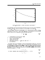
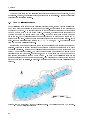
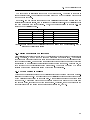
Download F50/51 Limnophysics - Physikalisches Institut Heidelberg

F50/51 Limnophysics
Version: March 2011
Sylvia Lorenz
Tillmann Kaudse
Prof. Dr. W. Aeschbach-Hertig
Abstract
During the practical course F50/51 the students perform measurements at Lake Willersinnweiher (an articial lake near Ludwigshafen). Temperature, conductivity and oxygen proles
at dierent locations within the lake are determined.
Based on these proles the mixing
behaviour of the lake is to be investigated.
In the second part of the practical course the students take water samples from the lake and
a groundwater sampling site to determine the groundwater inow into the lake. In order to
examine the interaction of groundwater with the lake, the radon concentrations of the samples
are measured in the hydrology lab of the Institute of Environmental Physics in Heidelberg.
Important notes:
ˆ
You won't be allowed to do this practical course if you cannot swim!
ˆ
This practical course starts on Monday at 9.00 a.m.
ˆ
In this instruction sheet all theoretical basics are included, so you do not need any
further literature.
Have you seen any mistakes during reading?
Please write an eMail to [email protected]
Contents
1 Motivation
5
2 Basics
7
2.1
2.2
Limnophysics
. . . . . . . . . . . . . . . . . . . . . . . . . . . . . . . . . . . .
Water density . . . . . . . . . . . . . . . . . . . . . . . . . . . . . . . .
7
2.1.2
Stratication of lakes . . . . . . . . . . . . . . . . . . . . . . . . . . . .
12
2.1.3
Stability of a water column
. . . . . . . . . . . . . . . . . . . . . . . .
16
2.1.4
Vertical mixing behaviour . . . . . . . . . . . . . . . . . . . . . . . . .
19
2.1.5
Oxygen content in lakes
. . . . . . . . . . . . . . . . . . . . . . . . . .
22
Radioactivity and radon . . . . . . . . . . . . . . . . . . . . . . . . . . . . . .
25
2.2.1
Decay series . . . . . . . . . . . . . . . . . . . . . . . . . . . . . . . . .
25
2.2.2
Decay law . . . . . . . . . . . . . . . . . . . . . . . . . . . . . . . . . .
25
2.2.3
Secular equilibrium . . . . . . . . . . . . . . . . . . . . . . . . . . . . .
27
2.3
Groundwater
2.4
Radon as a Tracer
2.5
. . . . . . . . . . . . . . . . . . . . . . . . . . . . . . . . . . . .
. . . . . . . . . . . . . . . . . . . . . . . . . . . . . . . . .
3.2
How does radon get into the groundwater? . . . . . . . . . . . . . . . .
30
How does radon get into lake water?
. . . . . . . . . . . . . . . . . . .
30
2.4.3
Henry's law . . . . . . . . . . . . . . . . . . . . . . . . . . . . . . . . .
30
Lake Willersinnweiher
. . . . . . . . . . . . . . . . . . . . . . . . . . . . . . .
2.5.1
Mixing behaviour in the last years
2.5.2
Oxygen content in the lake
CTD probe
33
. . . . . . . . . . . . . . . . . . . . . . . .
33
34
. . . . . . . . . . . . . . . . . . . . . . . . . . . . . . . . . . . . .
34
3.1.1
Design and functionality of the probe . . . . . . . . . . . . . . . . . . .
34
3.1.2
A short introduction to the software of the probe . . . . . . . . . . . .
34
Radon measurement instrument RAD7 . . . . . . . . . . . . . . . . . . . . . .
37
3.2.1
How the RAD7 works
. . . . . . . . . . . . . . . . . . . . . . . . . . .
37
3.2.2
Manual of the RAD7 . . . . . . . . . . . . . . . . . . . . . . . . . . . .
39
42
43
Measurements at Lake Willersinnweiher near Ludwigshafen
5.1.1
Materials
5.1.2
Measurements at the lake
. . . . . . . . . .
. . . . . . . . . . . . . . . . . . . . . . . . . . . . . . . . . .
. . . . . . . . . . . . . . . . . . . . . . . . .
44
44
45
Measurements in the hydrology lab . . . . . . . . . . . . . . . . . . . . . . . .
48
5.2.1
Groundwater measurement with the method RAD H2 0 . . . . . . . . .
48
5.2.2
Lake water measurement with the method RAD Aqua Plus
50
. . . . . .
6 Working tasks
6.1
32
. . . . . . . . . . . . . . . . . . . .
5 Implementation
5.2
29
2.4.2
4 Questions
5.1
29
2.4.1
3 Measuring instruments and techniques
3.1
7
2.1.1
Limnological parameters . . . . . . . . . . . . . . . . . . . . . . . . . . . . . .
54
54
3
6.2
Groundwater-lake interaction
. . . . . . . . . . . . . . . . . . . . . . . . . . .
7 Notes to the tasks
7.1
7.2
55
Analysis of the limnological parameters . . . . . . . . . . . . . . . . . . . . . .
55
7.1.1
Notes to task (1.1) . . . . . . . . . . . . . . . . . . . . . . . . . . . . .
55
7.1.2
Notes to task (1.2) . . . . . . . . . . . . . . . . . . . . . . . . . . . . .
56
7.1.3
Notes to task (1.3) . . . . . . . . . . . . . . . . . . . . . . . . . . . . .
56
Analysis of the groundwater-lake interaction . . . . . . . . . . . . . . . . . . .
56
7.2.1
Notes to task (2.1) . . . . . . . . . . . . . . . . . . . . . . . . . . . . .
56
7.2.2
Notes to task (2.2) . . . . . . . . . . . . . . . . . . . . . . . . . . . . .
57
Bibliography
4
54
57
1 Motivation
We are interested in lakes for many reasons.
People use lakes for relaxing after work, to
go hiking around them or to just sit on a bench and enjoy nature. Furthermore, lakes are
used for leisure time activities like swimming or shing. But lakes are not only important for
recreation, but also a very signicant ecosystem for plants and animals.
Humans sometimes disturb the ecological balance of lakes with their various activities.
To protect the ecology of lakes, it is important to know their limnological parameters. For
example, if the oxygen content is too low, the sh population of the lake will possibly die
o. So we need to know the oxygen content and how it is related to the mixing behaviour
of the lake.
One aim of this practical course is to examine the mixing behaviour of Lake
Willersinnweiher near Ludwigshafen and to determine the consequences for its ecosystem.
The second aim is to examine the inuence of the groundwater inow.
Figure 1.1: Lake Willersinnweiher and his neighbour gravel pit lakes, from Wollschläger [2003]
In this practical course two basic measurement techniques are applied: one limnological
and one hydrological technique.
To record the limnological parameters a probe is used to
measure temperature, conductivity and dissolved oxygen in dierent depths of the lake. In
the hydrological part, water samples from the lake and groundwater are taken and their radon
activity concentration is determined in the lab. The measurement techniques for the radon
measurement were developed at the Institute of Environmental Physics by T. Kluge [2005],
C. Ebert [2007], T. Reichel [2009] and many more.
5
1 Motivation
This practical course gives an overview on dierent elds of research and measurement
techniques of the Aquatic Systems group at the Institute of Environmental Physics.
The
research group is subdivided into
The
groundwater and paleoclimate
and
physical limnology.
members of the groundwater and paleoclimate group examine the noble gas concentration
in combination with the age of (ground-)water and analyse the signals with regard to paleoclimate. The members of the group physical limnology are interested in the mixing behaviour
of lakes with dierent sizes and shapes and their interaction with groundwater.
6
2 Basics
This chapter is similar to the lecture Physics of Aquatic Systems of Prof. Dr. W. AeschbachHertig [2007/2008]. Students who took part in the lecture will recognize the theory shown in
the next sections.
2.1 Limnophysics
Limnology deals with inland water and owing water. The word limnology has its origin in
the Greek word
limne,
which means lake and the Greek word
logos,
which means knowledge
or lore.
Limnology is mainly a biological subject and examines the structure and function of lakes
as ecosystems. To get a complete understanding of the processes in lakes, the physical and
chemical relations have to be known. For example, looking at a special kind of algae which
exists mainly in a depth of 3 m beneath the surface of the lake involves all three sciences.
The biologist detects the algae, but the reason for this special depth could not be explained
without the chemist and the physicist. One reason for this special depth is the right density
of the water, where the algae can oat easily and at the same time the luminosity is bright
enough to allow photosynthesis.
One part of general limnology is physical limnology which deals with the physical structures
and processes in lakes. One aim of physical limnology is to examine the mixing behaviour of
lakes. To get information about the mixing behaviour, the stability of a water column needs
to be known. The stability can be calculated with the help of water density.
2.1.1 Water density
The density
ρ
3
of a water body is dened as mass per volume and is given in kg/m .
m
ρ=
V
kg
(2.1)
m3
The density of water, like the density of other substances, depends on pressure and temperature. Additionally, the water density depends on the chemical (salt, dissolved substances, ...)
and physical (isotopes) composition. The water molecule has a polar structure and is therefore a good solvent. Some special properties of water are summarized in the following table
2.1.
The density
ρ
of water depends on the temperature
important for lakes.
T
in a special way which is very
Due to the anomaly of density, lakes freeze from the surface to the
ground. The water density in dierent lake depths is important for calculating the stability
of the water body. The stability values provide information about the vertical mixing which
is important e.g. for transporting oxygen to the lake bottom.
7
2 Basics
property
specic heat
comparison with
importance for the geosphere
other substances
and biosphere
higher than the specic heat
protects the environment from
of any other natural uid
extreme variabilities of
temperature
thermal expansion
fresh water has the highest
fresh water lakes are freezing
density at a temperature
from the surface to the ground,
above the freezing point
so sh can survive
(anomaly of density)
transparency
high, because the absorption
plants in greater depth are
of light in the visible
able to do photosynthesis
spectrum is small
heat conductivity
small
heat is transported mainly
through turbulences and not
through molecular diusion
Table 2.1: Properties of water, from Aeschbach-Hertig [2007/2008]
Density of pure water
The dependency of the density of pure water on temperature is not linear and it is not possible
to derive a theoretical equation. Chen and Millero [1986] give an empirical polynomial which
describes the density
ρ
3
(in kg/m ) of pure water:
ρ(T ) = 999, 8395 + 6, 7914 · 10−2 · T − 9, 0894 · 10−3 · T 2 + 1, 0171 · 10−4 · T 3
−1, 2846 · 10−6 · T 4 + 1, 1592 · 10−8 · T 5 − 5, 0125 · 10−11 · T 6
◦ C. This equation is applicable
◦
◦
of 1013 mbar and for temperatures between 1 C and 20 C.
Values of temperature
for a pressure
p
T
(2.2)
have to be put into the equation in
Usually the density of a substance decreases with increasing temperature because of the
characteristic thermal expansion. Water has a special behaviour because the breaking up of
the lattice structure of ice causes the volume to shrink, as the distance between the molecules
of water is shorter than the distance between the molecules of ice.
This process and the
thermal expansion overlap and lead to the density function of pure water (shown in gure
2.1).
Another possibility to describe the density is given by the thermal expansion coecient
α,
dened as
α(T ) = −
1 ∂ρ
ρ ∂T
K
−1
(2.3)
The thermal expansion coecient has a negative sign because an increase of density means
a contraction.
The thermal expansion coecient
α
for pure water changes its sign at the temperature of
Tρ,max (value is approximately 3,98 ◦ C). For lower temperatures the thermal
expansion coecient α is negative, for higher temperatures α is positive (shown in gure 2.2).
maximal density
8
2.1 Limnophysics
Figure 2.1: The density
ρ
p
of
of pure water as function of temperature
T
of pure water as function of temperature
T
at a pressure
1013 mbar
Figure 2.2: The thermal expansion coecient
at
p
α
= 1013 mbar, calculated as described in Chen and Millero [1986]
9
2 Basics
The density of salt water
The density of fresh water diers from the density of pure water because it additionally contains salts and dissolved gases. Usually the density is increased by dissolved salts and increased
or decreased by dissolved gases. Altogether the density can be described approximately as a
function of temperature and dissolved matter:
!
ρ(T, C1 , C2 , ...) = ρ(T ) ·
1+
X
β i Ci
(2.4)
i
ρ(T ), the dierent
βi dened as:
Thus, the salt water density depends on the density of pure water
concentrations of the substances
Ci
and the specic contraction coecient
1 ∂ρ
βi =
ρ ∂Ci
The specic contraction coecient
βi
"
g
−1 #
(2.5)
kg
describes the change of density by the change of
substance concentration and is dependent on temperature. Table 2.2 shows dierent values of
βi
at a temperature of
T
= 25
◦ C. Note that a negative signature indicates that the density
of the water will decrease when the concentration of the substance increases.
βi 10−3 kg/g
substance
Ca (HCO3 )2
0,813
Fe (HCO3 )2
0,838
NH4 (HCO3 )
0,462
CO2
0,273
NH4
-1,250
air
-0,090
particle with
ρ = 2, 65 g/cm3
= 1, 10 g/cm3
0,632
0,091
Table 2.2: Inuence of dissolved substances on the density of water, values from Imboden and
Wüest [1995]
In general mainly salts are dissolved in lake water. Therefore, only the salts are considered
and the dissolved gases and other neutral substances are neglected in the following calculations. To sum up all salts, a new parameter is introduced: the salinity
S
dened as the mass
of all salts in a volume per total mass of the volume.
mass of all salts in a volume of water
S=
total mass of the volume of water
g
kg
(2.6)
The salinity inuences the density. To get a qualitive value of the inuence, the coecient
of haline contraction
βS
is dened as
1 ∂ρ
βS =
ρ ∂S
10
"
g
kg
−1 #
(2.7)
2.1 Limnophysics
The value of
βS
−3 to 1·10−3 (g/kg)−1 . The coecient of haline concen-
varies from 0,73·10
tration diers from lake to lake, but the value can be approximated if the dominating salts are
known. Now it is possible to calculate the density as a function of temperature and salinity:
ρ(T, S) = ρ(T ) · (1 + βS S)
(2.8)
The probe used in this practical course does not directly measure the salinity
electrical conductivity
κ.
S,
but the
The electrical conductivity of a solution is dened as the reciprocal
value of the specic electrical resistance
ρS .
The unit Siemens S is equal to the unit
1
κ=
ρS
Ω−1 .
1
S
=
Ω·m
m
(2.9)
The measured in-situ conductivity is dependent on temperature and salinity. One aim of
the practical course is to compare values of the salinity in dierent depths. Therefore, it is
necessary to calculate the in-situ conductivity to a reference conductivity
◦
of 20 C. Bührer and Ambühl [1975] give an empirical polynomial for
κ20 at a temperature
κ20 , applicable for lakes
with calcium bicarbonate as the dominating salt.
κ20 = κT · 1, 72118 − 0, 0541369 · T + 1, 14842 · 10−3 · T 2 − 1, 222651 · 10−5 · T 3
κT [µS/cm]
with the electrical conductivity
and the measured temperature
Now we can derive the relation between salinity
S
T
(2.10)
◦
[ C].
and reference conductivity
κ20 :
the
salinity will increase linearly with the salt concentration if it is a highly diluted solution:
S = η · κ20
The value of
η
0, 87
0, 87 (mg/l) (µS/cm)−1 for lakes dominated by
conductivity increases by 1 µS/cm, the salinity will
is approximately
bicarbonate. This means, if the
by
(2.11)
calcium
increase
mg/l.
Like the coecient of haline contraction, the coecient of the reference conductivity
βκ
is
dened as:
1 ∂ρ
βκ =
ρ ∂κ20
After a short calculation, the equation
of the reference conductivity
βκ
"
µS
−1 #
(2.12)
cm
βS = βκ /η is derived. The value of the coecient
0, 707 · 10−6 (µS/cm)−1 for lakes containing
is calculated to
mainly calcium bicarbonate.
Now the relation between the salinity
S
and the reference conductivity
κ20
(equation 2.11)
as well as the connection between both contraction coecients are inserted in the density
equation 2.8. With this we have an expression of the density as function of the in-situ temperature and the reference conductivity which can be calculated from the in-situ conductivity
measured by the probe:
ρ(T, κ20 ) = ρ(T ) · (1 + βκ κ20 )
(2.13)
11
2 Basics
2.1.2 Stratication of lakes
One of the main aspects of physical limnology is the vertical layering, called stratication. If
the temperature is dominating the density, the lake is called thermally stratied. In gure
2.3 three layers are drawn in the temperature prole. The epilimnion is the upper layer with
well mixed water because of the wind. In the middle layer, which is called the thermocline or
metalimnion, the temperature decreases. The deepest layer is the hypolimnion.
The density is mainly inuenced by temperature. Therefore, it is possible to subdivide the
lake into three layers according to the temperature prole. For lakes with a high salt content
this approximation is not possible. In this case the characterisation of epilimnon, metalimnion
and hypolimnion has to be done with the help of the density prole.
Figure 2.3: Characterisation of the dierent lake layers, from Schönborn [2003]
Surfaces of equal density are called isopycnals.
In lakes, isopycnals are approximately
horizontal. Within isopycnals no work is needed to mix water. Therefore, horizontal mixing
processes are relatively fast and we consider lakes as horizontally homogeneous.
mixing needs energy because work against gravity has to be done.
Vertical
Therefore, vertical or
so-called diapycnal mixing is much slower (for further information refer to chapter 2.1.4).
The stratication of lakes changes with the seasons due to dierent solar radiation uxes.
Lakes get their energy mainly through the surface. Therefore, the surface temperature of a
lake depends extremely on the seasonal variations of the solar energy ux. In gure 2.4 the
seasonal changes of the energy ux and the surface temperature of lakes for dierent latitudes
are shown.
In our latitude the solar ux has its maximum during summer.
The surface
temperature reaches its maximum a little later during the late summer months. Figure 2.5
shows a typical seasonal change of stratication.
12
2.1 Limnophysics
Figure 2.4: Seasonal change of solar ux and surface temperature, from Hostetler [1995]
Figure 2.5: Seasonal change of stratication in a dimictic lake, from Schwoerbel and Brendelberger [2005]
Figure 2.6: Circulation only in the epilimnion (left) and the starting circulation in the hypolimnion (right), from Schönborn [2003]
13
2 Basics
During summer the temperature of the epilimnion increases due to the increasing solar ux.
Lake water absorbs the energy of the sun, but radiation reaches only some meters down and
causes no direct heating of water in the deeper part. The thermocline is the layer in which
only a small part of the light arrives.
Thus, the temperature in the thermocline decreases
strongly. In the deeper part, the hypolimnion, lake water with the highest density is found.
In deep lakes the temperature of the hypolimnion is approximately 4
◦ C. In this case we speak
of a thermally stratied lake or the summer stagnation. Only the epilimnion is well mixed
because of the wind (shown in gure 2.6 on the left side).
In autumn the solar ux is smaller than in summer. Therefore, the surface temperature
decreases until it reaches approximately 4
◦ C. In this situation the wind is able to mix the
lake completely (shown in gure 2.6). After a complete circulation the temperature of the
lake is equal in every depth. This situation is called a homothermal lake.
During winter the surface temperature can decrease to values below 4
◦ C and the water at
the surface can freeze. The ice or cold water stays above the water with a temperature of 4
◦ C due to the density anomaly of water (shown in gure 2.1). In this situation, called inverse
stratication, the eplilimnion cannot mix with the hypolimnion without an input of energy. If
the temperature at the surface decreases below the freezing point, the ice layer insulates the
lake water. Therefore, the ice layer grows only slowly from the surface to the ground. This
eect is very important, because it protects the sh and other animals in the lake.
In spring the ice melts and a homothermal situation is reached again because of the increasing solar ux. Now the wind causes a second complete circulation of the lake. Lakes which
mix in autumn and spring are called dimictic lakes. There are other types of lakes which mix
only once a year (mainly in spring).
Lakes can be classied according to their annual mixing behaviour.
There are amictic,
holomictic, dimictic, polymictic and meromictic lakes. Amictic lakes never circulate because
they are permanently frozen or thermally stratied. Examples are lakes in the Arctic (Greenland), in the Antarctic and in the tropics.
Holomictic lakes completely mix once, dimictic
lakes twice and polymicitic lakes many times a year.
Polymictic lakes are often relatively
shallow.
Meromictic lakes do not mix completely over a long time period. In meromictic lakes a deep
layer can be found, the monimolimnion, which does not take part in a circulation event for a
long time. The layers above, which take part in the seasonal circulation, can be summarised
as mixolimnion. This special type of stratication is often caused by a high salinity in the
monimolimnion.
Because of the high salinity the density of the monimolimnion is much
higher than the density of the mixolimnion even if the temperature of the mixolimnion is
approximately 4
◦ C.
In the following gures the temperature or conductivity proles for dierent lake types are
shown. Lake Alpnach (a part of Lake Lucerne) is a holomictic lake. From gure 2.7 we can
conclude that it completely mixed in the spring of 1992.
14
2.1 Limnophysics
0
6
Depth (m)
12
Lake Alpnach 1992
18
Jan.
Mar.
May
Jul.
Nov.
24
30
0
5
10
15
20
25
Temperature (°C)
Figure 2.7: Temperature prole of Lake Alpnach, from Kipfer et al. [2002]
A meromictic lake is, for example, the articial lake Merseburg-Ost 1b (Lake Raÿnitz) in
Germany. Figure 2.8 shows that the temperature below 57 m a.s.l. (above sea level) stays
constant over the whole year. The temperature in the mixolimnion decreases to approximately
4
◦ C meaning that the temperature of the monimolimnion is higher than the temperature of
the mixolimnion. This situation can only be explained by extraordinary high salinity in the
Fig. 10
monimolimnion which stops the mixing. The high salinity causing the long-time stability of
the monimolimnion is shown in the right part of the gure.
Figure 2.8: Temperature and conductivity proles of Lake Merseburg-Ost 1b, from [von Rohden and Ilmberger, 2001]
15
2 Basics
2.1.3 Stability of a water column
In the section above the vertical stratication of lakes was discussed qualitatively. Now, the
Brunt-Väisäla frequency will be introduced to get a quantitative measure for the stability of
a water column.
A column of water is called stable, if a water parcel, which is deected from its equilibrium
state, experiences a restoring force. Looking at a water parcel and its surrounding water the
density of the water parcel
ρP
and the surrounding water
ρU (z0 )
are equal at the depth
(equilibrium state). If the water parcel is lifted upwards a small distance
(z − z0 )
z0
(shown in
gure 2.9), the following forces act on the water parcel (z coordinate positive upwards):
gravity:
FG
= −gρP V
(2.14)
buoyancy:
FA
= gρU V
(2.15)
force:
acceleration:
Fsum = FG + FA
Fsum = −g(ρP − ρU )V
Fsum
a
=
ρP V
(2.16)
(2.17)
Figure 2.9: Lifted and equilibrium state of a water package
Therefore, we get the restoring force per unit of mass acting on the water parcel:
z̈ = −g
ρP − ρU (z)
ρP
(2.18)
ρU (z) at the lifted depth z is almost equal to the density of the surrounding water ρU (z0 ) at the depth z0 . Therefore, a Taylor series approximation
The density of the surrounding water
is possible:
ρU (z) ≈ ρU (z0 ) +
16
dρ
dz
(z − z0 )
(2.19)
2.1 Limnophysics
This approximation is put into equation 2.18. Further, we consider that the density of the
water parcel
ρP
is equal to the density of the surrounding water
ρU (z0 )
in the equilibrium
state. We derive the restoring force per unit of mass:
g
z̈ =
ρP
dρ
dz
(z − z0 )
(2.20)
This is the well-known dierential equation of a harmonic oscillation oscillator.
z̈ = −N 2 (z − z0 )
(2.21)
with the oscillation frequency N
N2 = −
g
ρP
dρ
dz
(2.22)
As discussed in chapter 2.1.1 the density of water is a function of temperature and salinity.
Hence, the density gradient can be split up using equations 2.3 and 2.7.
dρ
dz
∂ρ ∂T
∂ρ ∂S
+
∂T ∂z
∂S ∂z
∂T
∂S
= −αρ
+ βρ
∂z
∂z
=
(2.23)
(2.24)
Now it is visible that the stability frequency has also two components:
∂T
∂S
N2 = g α
−β
∂z
∂z
(2.25)
= NT2 + NS2
Let's have a closer look at the derivation.
(2.26)
So far we neglected that the temperature of
the water parcel decreases as it is lifted up, because the pressure decreases.
of the decompression the water parcel will expand, thereby spending energy.
the temperature will decrease. The adiabatic temperature gradient
(dT /dz)ad
As a result
Therefore,
describes this
change of temperature:
dT gTabs α
=−
= −Γ(T, S, p)
dz ad
cp
g
gravity constant
Tabs
cp
Γ(T, S, p)
α
in-situ temperature in Kelvin
(2.27)
specic heat capacity
adiabatic temperature gradient
coecient of thermal expansion
Therefore, it is necessary to compare two water parcels at the same reference depth. The
potential temperature
Θ(z, z0 )
is the temperature of a water parcel from the depth
lifting it adiabatically to the depth
z0 ,
z
after
correcting the depth dependency of temperature:
17
2 Basics
Z
z0
Θ(z, z0 ) = T (z) −
Γ Θ(z, z 0 ), S(z), p(z 0 ) dz 0
(2.28)
z
For temperatures above 4
◦ C it is possible that the temperature increases a little bit with
depth but the water column is still thermally stratied. Therefore, for a correct calculation
of the stability frequency we have to use the potential temperature instead of the in-situ
temperature. During the derivation of the Brunt-Väisäla frequency we split up the density
gradient. At this point of the calculation we have to put in the potential temperature instead
of the in-situ temperature:
dρ
∂ρ ∂Θ
∂ρ ∂S
=
+
dz
∂Θ ∂z
∂S ∂z
(2.29)
The partial derivative of the potential temperature can be deduced from equation 2.28:
∂T
∂Θ
=
−
∂z
∂z
∂T
∂z
(2.30)
ad
The adiabatic temperature gradient for lakes is usually small enough to be neglected. Therefore, we can use the in-situ temperature instead of the potential temperature for our lake.
This approximation is not allowed in deep lakes and the ocean.
Interpretation of the Brunt-Väisäla frequency
The inverse of the Brunt-Väisäla frequency
N
is the oscillation period of a water package
deected by a small distance from its equilibrium state. We consider that there is no exchange
with the surrounding water during the oscillation. The Brunt-Väisäla frequency squared,
N 2,
is a quantitative measure for the stability of a water column:

 >0
=0
N2 =

<0
For negative density gradients, i.e.
stable
labile
unstable
if there is lighter water above heavier, the square of
the Brunt-Väisäla frequency is positive and the water column is stable. For positive density
gradients the value of
N2
is negative and the water column is instable.
The stratication is more stable if the density gradient is greater. Therefore, in a strongly
stratied lake turbulences will calm down quickly.
NT2 and NS2 . If the density
2
2
gradient is dominated by temperature the stability N is almost equal to NT . If the density
2
2
2
gradient is dominated by salinity the stability N is almost equal to NS . Usually NT dominates
2
in the thermocline while NS characterizes stability in the hypolimnion.
The Brunt-Väisäla frequency consists of two components:
NT2 , may indicate instability in the mon2
2
that NS is much greater than NT and nally
In meromictic lakes the temperature component,
imolimnion, but the salinity is high enough so
leads to a positive
N2
which corresponds to a stratication.
in the salinity component,
NS2 ,
Because of the high stability
the monimolimnion cannot take part in the circulation. An
example for this situation is shown in gure 2.10 below 60 m a.s.l.
For further information about stability take a look at Millard et al. [1990] or Wüest et al.
[1996].
18
2.1 Limnophysics
Figure 2.10: Stability of a water column
N 2,
and its components, for Lake Merseburg-Ost
from von Rohden and Ilmberger [2001]
2.1.4 Vertical mixing behaviour
Overview
Lakes mix because of many reasons. One reason for mixing are wind-driven currents. Accelerated water with a certain velocity rubs against deeper water with low velocity. Therefore,
we get a velocity gradient which causes turbulences and mixing. Another reason for mixing
is an unstable water column which causes convection and turbulences.
By speaking of horizontal and vertical mixing we mean mixing along isopycnal and diapycnal
surfaces. Isopycnal mixing means mixing within a density layer (density layers in lakes are
almost horizontal) while diapycnal mixing takes place perpendicularly to a density layer.
During isopycnal mixing we have a energy loss only due to friction. Diapycnal mixing needs
energy to move water against the gravity. Therefore, isopycnal mixing coecients are about
ten or hundred times bigger than diapycnal mixing coecients.
In a stratied lake mixing in the hypolimnion will mainly be caused by eddy diusion and
molecular diusion. Eddy diusion results from horizontal currents along dierent layers (for
example sediment, isopycnals, ...). These small eddys cause further small eddys and a heat
exchange is reached.
Molecular diusion needs a concentration gradient and causes also a
heat exchange.
19
2 Basics
The eddy and molecular diusion together with further mixing processes - which are described in Imboden and Wüest [1995] - are included in the mixing coecient
Kz ,
which is
also called turbulent diusion coecient. There are many methods to determine the mixing
coecient. With our equipment we get the best results with the budget-gradient method.
Budget-gradient method
The budget-gradient method is based on the change of a parameter (for example temperature)
below a certain depth caused by the vertical ux. We will derive the mixing coecient by
connecting the amount of heat below a layer and the vertical temperature gradient.
The budget-gradient method assumes a horizontally homogeneous lake with no vertical
advection. Now we can calculate the amount of heat
z0
and the maximum depth
prole
T (z)
zm
W (z0 )
in the layer between the depth
by integration. We integrate the product of the temperature
and the cross-section area prole
A(z)
Z
of the lake:
z0
W (z0 ) = cp ρ
A(z)T (z)dz
(2.31)
zm
The amount of heat in the layer changes over time. We can calculate this change of heat by
dierentiating the equation with respect to time. In the following step we take into account
that we can exchange integration and dierentiation:
∂W (z0 )
= cp ρ
∂t
Z
z0
A(z)
zm
∂T (z)
dz
∂t
In gure 2.11 the transport of heat through the area
perature proles
t1
and
t2
is shown.
(2.32)
A(z0 ) during the time between tem∆ transported by diusion has
The amount of heat
increased the amount of heat and thus the temperature in the lower layer.
Figure 2.11: Diusive transport of heat through the area
A(z0 ),
Systems I of Prof. Aeschbach-Hertig [2007/2008]
20
from the lecture Aquatic
2.1 Limnophysics
Below a certain depth we can assume a ux of heat
Fth
only caused by diusion and not
by advective transport or radiation. This vertical heat ux based on turbulent diusion is
described by Fick's rst law:
Fth = −cp ρKz
Fth
cp
ρ
Kz
thermal ux of energy per area and time
∂T
∂z
vertical temperature gradient
∂T
∂z
(2.33)
specic heat
density
vertical mixing coecient
We get the additional amount of heat per time by multiplying the thermal ux
cross-sectional area
A(z0 )
Fth
with the
through which it passes. The heat ux in equation 2.33 describes
the thermal ux in upward direction (z is positive upwards). We are interested in the change
of heat in the volume below the depth
z0 ,
so we consider this information of direction with
the negative sign. The equation for the complete heat ux into the volume below the depth
z0
is:
∂W (z0 , t)
∂t
= −A(z0 ) · Fth (z0 )
(2.34)
∂T (z, t) = A(z0 )cp ρKz (z0 )
∂z z0
In a rst step we solve the equation for the mixing coecient
Kz .
In a second step we
insert equation 2.32 into the solved equation and get the following dependency:
Kz (z0 ) =
∂W (z0 ,t)
∂t
(z,t) A(z0 )cp ρ ∂T∂z
z
R z0
=
(z,t)
dz
A(z) ∂T∂t
(z,t) A(z0 ) ∂T∂z
zm
(2.35)
z0
0
During this practical course the gradient is calculated from the change of two temperature
proles
t1
and
t2
which are taken at two dierent dates during the year. For the calculation
of the mixing coecient we therefore take the following equation:
Kz (z0 ) =
R z0
∆W (z0 ,t)
∆t
=
(z,t) A(z0 )cp ρ ∂T∂z
z
0
(z,t)
A(z) ∆T∆t
dz
(z,t) A(z0 ) ∂T∂z
zm
(2.36)
z0
with
∆t = t2 − t1
∆W (z0 ) = W (z0 , t2 ) − W (z0 , t1 )
∂T (z, t) ∂z z0
=
1
2
!
∂T (z, t1 ) ∂T (z, t2 ) +
∂z
∂z
z0
z0
21
2 Basics
Relationship between stratication and vertical diusion
Stratication and vertical diusion correlate. The relationship of the Brunt-Väisäla frequency
N2
and the mixing coecient
Kz
can be described after von Rohden et al. [2007]:
Kz = a · N 2
−b
(2.37)
Typical values of the parameters a and b for Lake Willersinnweiher (near Ludwigshafen) were
determined by von Rohden et al. [2007]:
a
=
b
=
(2, 5 ± 0, 6) · 10−10
0, 81 ± 0, 02
2
3
m /s
Equation 2.37 shows that the stratication is stronger if the vertical turbulence is weaker.
More information about this subject can be found in the papers of Quay et al. [1980], Jassby
and Powell [1975] and Wüest et al. [2000].
2.1.5 Oxygen content in lakes
There are many processes which change the oxygen content of lakes. Oxygen gets into the
surface water mainly by gas exchange of the surface water with the atmosphere. A further
important oxygen source are green plants and cyanobacteria (blue-green algae), which perform
photosynthesis. Production of oxygen by photosynthesis is dependent on light. Water absorbs
light, therefore oxygen can only be produced in the upper layers. The deep hypolimnion is
reached by almost no sunlight and thus it is not possible to produce oxygen there. In contrast,
oxygen consuming processes are going on.
In the epilimnion the algae grow due to photosynthesis. When algae die they sink to the
hypolimnion, where these organic substances are decomposed by bacteria. The decomposition
is an oxygen consuming process.
The oxygen in the hypolimnion which is needed for this
process is mainly the oxygen of the last circulation in which the deep water exchanged oxygen
with the atmosphere. The oxygen decrease starts with the stagnation of the water body.
The oxygen content in the hypolimnion is dependent on dierent constraints: Oxygen in
the hypolimnion can only get there by mixing with the epilimnion.
Therefore, the mixing
type of the lake is very important for the oxygen content. A meromictic lake has no oxygen in
the monimolimnion as the water of the monimolimnion has no contact to the atmosphere and
the oxygen inow by the groundwater is usually negligible. In a holomictic lake the amount
of oxygen depends on the volume of the hypolimnion. A bigger hypolimnion can store more
oxygen.
The strength of oxygen consumption depends on how much organic substances from the
epilimnion sink to the deeper layers where they are decomposed. In a lake with only small
organic production in the epilimnion it is possible that most of the organic substances are
decomposed before they have reached the hypolimnion. Therefore, only little oxygen is consumed in the hypolimnion. The velocity of the decomposition of organic substances depends
on temperature.
At higher temperatures more organic substances are decomposed than at
a lower temperature in the same time. Further, we have to consider that at higher temperatures the absolute content of dissolved oxygen is smaller than at lower temperatures (see
22
2.1 Limnophysics
Figure 2.12: Seasonal change of the oxygen content, from Schönborn [2003]
23
2 Basics
section 2.4.3). Therefore, the oxygen content will decrease faster at higher temperatures. The
oxygen prole in a lake has a characteristic seasonal change which is shown in gure 2.12.
During summer stagnation there are two typical oxygen proles: the orthograde and the
clinograde distribution of oxygen. The shape of the orthograde oxygen prole is similar to
the oxygen prole after a full circulation. That means the oxygen content is nearly constant
in every depth.
An orthograde oxygen prole can be found in deep holomictic lakes with
only small production of organic matter.
productivity are called oligothrophic.
Lakes with low nutrient contents and hence low
The clinograde oxygen prole has a higher oxygen
content in the epilimnion and a very low oxygen content in the hypolimnion. The decrease
of oxygen with depth does not have to be continuous. It is possible that there are maxima
and minima due to biological activity.
A clinograde oxygen prole can often be found in
nutrient-rich and thus highly productive lakes, which are called eutrophic lakes.
Figure 2.13 shows some examples.
In part A the orthograde oxygen prole of the olig-
othrophic Königsee is shown from 5.7.1980. In part B and C two clinograde oxygen proles
are shown. Part B shows the oxygen prole of the deep, eutrophic Lake Biel in Switzerland
from 11.10.1976 and part C shows the oxygen prole of the eutrophic Puÿsee in Holstein
which is sheltered from the wind (prole taken on 4.9.1989).
Figure 2.13: Orthograde and clinograde oxygen proles, from Lampert and Sommer [1999]
24
2.2 Radioactivity and radon
2.2 Radioactivity and radon
2.2.1 Decay series
Radioactivity is a characteristic of unstable nuclei.
They are able to transform themselves
into an nucleus with a lower energetic level by emitting a characteristic radiation. In table
2.3 the three types of radiation are summarized.
type of decay
α decay
β − decay
γ decay
transform process
A X → A−4 Y + 4 He
2
Z
Z−2
AX → A
−+ν
Y
+
e
Z
Z+1
A X∗ → A X + h · ν
Z
Z
emission
helium nucleus (α-radiation)
electron, antineutrino
γ -radiation
Table 2.3: The three types of radiation
An unstable nucleus can decay into a stable nucleus or into another unstable one. Therefore,
decay series can arise. Altogether only four dierent
do not change the mass number but the
α
α-decay series exist, because β or γ decays
decay decreases the mass number by four units for
each decay. Today only three of the four decay series can be detected: the Thorium series,
the Uranium-Radium series and the Uranium-Actinium series. The Neptunium series with a
half-life of the starting isotope of 2,14 million years has already almost completely decayed.
Radon and its isotopes can be found in all three of the natural radioactive decay series,
which is shown in gure 2.14.
The dierent radon isotopes have dierent half-lives.
222 Rn, which is sometimes called
238 U decay series has a half-life of 3,82 days. The isotope 220 Rn, which is
radon, from the
232 Th decay series has a much smaller half-life of 55,6 seconds and the
called thoron, from the
isotope
219 Rn, which is called actinon, from the 235 U decay series has a even smaller half-life
of 3,9 seconds.
The radioactive noble gas radon is colourless, odourless and shows a negligible reactivity
with other elements. Thus, it is suitable for the use as a tracer (see section 2.4), for example,
for the interaction between groundwater and lake water. The processes we look at take place
in a time range of hours or days and thus we choose radon as a tracer due to its suitable
half-life.
2.2.2 Decay law
The radioactive decay is a statistical process, which can be described by the radioactive decay
law (equation 2.38). The number
N (t) of nuclei of a radioactive material at time t which have
not yet decayed decreases exponentially with time:
N (t) = N0 · e−λt
N0
λ
(2.38)
initial number of nuclei of the radioactive material
decay constant
25
2 Basics
Figure 2.14: The three natural decay series, from Kluge [2005]
The half-life
T1/2
is the time after which the number of nuclei is halved.
N (T1/2 ) = N0 · e−λT1/2
−λT1/2
−λT1/2
T1/2
N0
2 1
= ln
2
= − ln (2)
ln 2
=
λ
=
(2.39)
Radon has a half-life of 3,82 days. Therefore, after two half-lives or approximately eight
days only 25% of the original amount of radon can be measured. So, the radon measurements
should be done in a short time after taking the water samples.
The activity
A
of a radioactive material describes the number of decays per time.
A(t) = −
26
dN (t)
= λN (t)
dt
(2.40)
2.2 Radioactivity and radon
The unit of the activity is Becquerel (Bq), Curie (Ci) or pico Curie (pCi =
10−12
Ci). One
Becquerel is equal to one decay per second. One Curie is equal to the activity of 1 g
1
Ci
= 3, 7 · 1010
226 Ra:
Bq
(2.41)
In this practical course we will measure activity concentrations that refer to the activity of
a certain water volume.
2.2.3 Secular equilibrium
We will determine the radon concentration of water by using the measurement instrument
RAD7. The RAD7 is not able to measure the radon activity concentration directly, but it can
measure the decay products of radon. Therefore, we derive the relationship between radon
and polonium in this section.
If we look at a small decay series of a mother nucleus
N1
and a daughter nucleus
N2 ,
the
mother nucleus will decay according to the radioactive law (dierential version):
−
dN1 (t)
= λ1 N1 (t)
dt
(2.42)
The amount of daughter nuclei is dependent on the amount of recently decayed mother
nuclei and is also dependent on the decay of daughter nuclei itself. The change of the amount
of daughter nuclei can be described in the following way:
dN2 (t) = λ1 N1 (t)dt − λ2 N2 (t)dt
(2.43)
If we now insert the dependency between the number of decays
N
A,
and the activity
described in equation 2.40, we get the activity of the daughter nucleus
as
A2 :
dA2
= λ2 (A1 − A2 )
dt
(2.44)
This dierential equation is solved in Wilkening [1990]. By taking the starting conditions
A1 (0) = A01
(2.45)
A2 (0) = 0
(2.46)
into consideration the solution is
A2 (t) =
λ2
· A01 · e−λ1 t − e−λ2 t
λ2 − λ1
Figure 2.15 shows the activity of the mother nucleus Radon-222 (T1/2
and the daughter nucleus Polonium-218 (T1/2
= 3, 05
min).
(2.47)
= 5500, 8
min)
We infer that after a time
t
of approximately 20 minutes the equilibrium state is reached and that the activity of the
daughter nucleus is nearly constant. This equilibrium is called secular equilibrium.
The equilibrium state can be explained mathematically by the dierent half-lives.
half-life
T1
of radon is much bigger than the half life
T2
The
of polonium. Therefore, the decay
constant of radon is much smaller than the decay constant of polonium (λ1
<< λ2 )
and we
can make the following approximation:
λ2 − λ1 ≈ λ2
(2.48)
27
2 Basics
1 2 0
1 1 0
1 0 0
9 0
8 0
(B q )
6 0
A
7 0
5 0
4 0
3 0
R a d o n
P o lo n iu m
2 0
1 0
0
0
2
4
6
8
1 0
1 2
1 4
1 6
1 8
2 0
2 2
2 4
2 6
2 8
3 0
t (m in )
Figure 2.15: Secular equilibrium between the activity
the time
A
of
222 Rn and 218 Po in dependence of
t
After a period of time
t,
which is much longer than the half-life
T2 ,
the term
e−λ2 t
in
equation 2.47 is almost zero. With this approximations and the activity of the mother nucleus
A1 (t) = A01 · e−λ1 t
we derive mathematically the secular equilibrium:
A2 (t) = A1 (t)
(2.49)
In the case of a much bigger half-life of the mother nucleus than of the daughter nucleus
we will always see that the activity of both radioactive materials will be equal after a suitable
time t. The secular equilibrium is important for the calculation of the activity concentrations
of radon with our measurement instrument RAD7.
We reach the secular equilibrium between
222 Rn and 218 Po after 20 minutes. The secular
222 Rn and 214 Po (see gure 2.14) is reached after three hours.
equilibrium between
This
second secular equilibrium is considered for very exact measurements. During the practical
course we will mainly consider the equilibrium between
28
222 Rn and 218 Po.
2.3 Groundwater
2.3 Groundwater
Groundwater is subsurface water, which ows above or between a watertight aquitard in the
ground. Figure 2.16 shows the dierent zones of groundwater.
Figure 2.16: Groundwater zones, from Bear [1979]
The soil water zone (1) is a zone near the surface in which the roots of the plants hold
the water.
The water content of the soil water zone is dependent on precipitation.
Below
the soil water zone the intermediate or vadose zone (2) is located. There, water is kept by
capillary forces. However, the vadose zone is not saturated and we can nd air embedded in
pore spaces. At the lower part of the vadose zone the capillary fringe (3) is located. Water of
the capillary fringe rises from the saturated groundwater zone (4) due to capillary forces. The
groundwater level is the depth of the saturated groundwater zone in which the hydrostatic
pressure equals the atmospherical pressure.
Groundwater ow occurs in aquifers which are a system of connected pores, so that water
can ow slowly through it. Good aquifers are e.g. sediments of gravel, sand and sandstone.
2.4 Radon as a Tracer
In this practical course we will investigate in which depth groundwater straties into the lake
water.
This is done with the help of a tracer.
A tracer is a substance or a characteristic
property which marks a water body or water mass. We are therefore able to detect a certain
water mass. The group of tracers can be divided into natural and articial tracers. Natural
tracers are, for example, the isotopic composition of the water itself, the amount of heat
respectively the temperature of a water mass or - as in our case - the radon concentration of
the water. Articial tracers like SF6 have to be introduced deliberately into the system.
Radon is a noble gas with a very low chemical reactivity under natural circumstances.
Further, there is a big dierence in the concentrations of radon in lake and groundwater.
Thus, radon is a good tracer for the inow of groundwater into lakes.
Temperature is not
such a good tracer, because the as the temperature dierence is not as large and temperature
inuences density and hence the depth of interstratications of the inowing groundwater.
29
2 Basics
2.4.1 How does radon get into the groundwater?
Radium is the mother nucleus of radon and is abundant in every type of sediment or rock in
dierent concentrations. Radium decays to radon inside the ground or sediment and leaves
the sediment grains due to the recoil from the decay (conservation of linear momentum) (see
Dehnert et al. [1999]). Another possibility is that radon diuses through the sediment into
groundwater, where it accumulates.
In a homogeneous sediment a characteristic radon activity concentration can be calculated.
Sandler [2000] shows that the value of the characteristic radon activity concentration for a
3
sand and gravel aquifer is approximately 9 000 Bq/m .
2.4.2 How does radon get into lake water?
There are dierent origins of radon in lake water.
Inows and precipitation as well as the
surface water are in contact with the atmosphere, thus their radon concentration is determined
by the solubility equilibrium (see below). Since the atmosphere has no radon sources but only
the sink due to decay, its radon content and thus that of surface water is very low. A further
origin of radon in lakes is diusion from the sediments. Another source is the decay of dissolved
radium in the lake water.
And nally radon in lake water originates from groundwater, if
there is an inow of groundwater into the lake.
Altogether the radon concentration in lake water is much lower than in groundwater due
to rstly the exchange of the surface water with the atmosphere and secondly the quite fast
decay.
2.4.3 Henry's law
We take a look at a system of two phases, for example air and water. In this system we add
a gas, in our case radon. A part of this gas will dissolve into the water and the other part
will stay in the air. If we wait a sucient period of time we will see that the gas reaches a
dynamical equilibrium state, which means that the ux of radon from air to water equals the
ux the other way round.
The amount of gas dissolved in the water phase depends on the solubility of the specic
gas and other factors.
The dimensionless Ostwald solubility,
a,
describes the ratio of the
equilibrium concentration of the gas in the uid to the concentration in the gas phase:
a=
a
Cf l
Cg
Cf l
Cg
(2.50)
Ostwald solubility
activity concentration in the uid phase
activity concentration in the gas phase
The solubility of radon is dependent on temperature. This dependency was found empirically by Weigel [1978]:
a(T ) = 0, 105 + 0, 405 · e−0,0502·T
In equation 2.51 the temperature,
T,
has to be put in in
(2.51)
◦ C. For example, if we calculate
◦
◦
the solubility at a temperature of 20 C we get a value of 0,25. That means that at 20 C
30
2.4 Radon as a Tracer
0 ,6
0 ,5
a
0 ,4
0 ,3
0 ,2
0 ,1
0 ,0
0
2
4
6
8
Figure 2.17: Solubility
1 0
a
1 2
1 4
1 6
1 8
T (°C)
2 0
2 2
2 4
2 6
2 8
of radon dependent on temperature
3 0
T
the concentration in the gas phase is four times higher than in the uid phase at equilibrium
conditions. Figure 2.17 shows the dependency of the solubility on temperature.
In the equilibrium state the gas concentration in the water phase is dependent on its concentration in the gas phase
Cg
(see equation 2.50).
The concentration of the gas phase is
further dependent on the pressure as described in the ideal gas law:
Cg =
Cg
n
p
=
V
RT
(2.52)
concentration in the gas phase in mol/liter
n
number of mols of the substance
V
volume of the gas in liter
p
pressure of radon in atm
R
ideal constant for gas ( R = 0,08206 atm liter mol
T
temperature in K
−1 K−1 )
Henry's law states the proportionality of the gas concentrations in a liquid and a gas phase
in equilibrium, as expressed by equation 2.50. Often, it is expressed as a relationship between
the concentration of the dissolved gas in the uid
p.
Cf l
and the partial pressure in the gas phase
We can derive Henry's law in that form from equations 2.50 and 2.52. There are dierent
possibilities to write Henry's law. The rst and commonly used possibility is with the help of
the Henry coecient
KH = RT /a:
p = Cf l · KH
The second possibility uses the solubility coecient
Cf l = KS · p
(2.53)
KS = a/(RT ):
(2.54)
31
2 Basics
The Henry coecient and the solubility coecient are dependent on temperature, but not
on pressure. Further, the solubility of radon is dependent on the salinity. Usually the solubility
decreases with increasing salinity.
2.5 Lake Willersinnweiher
Lake Willersinnweiher is one of four articial (dredging) lakes, located between Friesenheim
and Oppau near Ludwigshafen in the upper Rhine Valley. It was created in the beginning of
the 1930s by the BASF. The gravel pit reached to the upper groundwater layer (which reaches
down to a depth of 25 m in the Rhine Valley). Therefore, the groundwater is connected to
the lake and lled the gravel pit up with water.
Soon the newly formed lake was used
for swimming. Lake Willersinnweiher has no surface inows or outows and is only fed by
groundwater and rain. Groundwater in the surroundings of the lake ows from south-west to
north-east with a relatively slow velocity of
6, 1 · 10−3
m/d to 0,45 m/d. The values are taken
from the model of Wollschläger [2003].
During autumn 1975 the lake suered from a oxygen depletion which required an emergency
aeration. After this emergency aeration the morphology of the lake was reshaped to improve
the lake's ventilation.
Before Lake Willersinnweiher was reshaped it was divided into two
parts by an underwater barrier. The height of this barrier was decreased to enable a deep
circulation between both parts. Furthermore, the mud of the sediment was dug out and the
lake reached its present maximum depth of 20 m.
In 1989 Lake Willersinnweiher got its
ocial permission to be used as a swimming lake. As a consequence the shore of the lake was
reshaped with some small isles. In gure 2.18 the recent morphology of Lake Willersinnweiher
is shown.
Figure 2.18: The morphology of Lake Willersinnweiher. The barrier is marked by a red line.
From Wollschläger [2003]
32
2.5 Lake Willersinnweiher
The lake bottom is irregularly shaped with a very steep shore. The shape of the shore is
almost a straight line. The red line in the gure marks the 8 m depth barrier which impedes
the deep water exchange.
In table 2.4 some important parameters of Lake Willersinnweiher are summarized from the
dissertations of Sandler [2000], Schmid [2002] and Wollschläger [2003]. Lake Willersinnweiher
is a hard water lake with lots of calcium. Thus, the equations derived in chapter 2.1.1 are
valid for Lake Willersinnweiher.
geographical parameters
volume
1, 3 · 106 m3
surface area
mean depth
maximum depth
maximum length
maximum width
16 − 17
7, 7 m
20 m
850 m
325 m
ha
typical amounts of ions in the lake water
sulfate
bicarbonate
chloride
sodium
calcium
nitrate
2, 4 mmol/l
2, 3 mmol/l
2, 2 mmol/l
1, 9 mmol/l
2, 5 mmol/l
30 µmol/l
Table 2.4: Parameters of Lake Willersinnweiher summarized from Sandler [2000], Schmid
[2002] and Wollschläger [2003]
2.5.1 Mixing behaviour in the last years
Lake Willersinnweiher has been examined by the Institute of Environmental Physics for several
years.
Therefore, we know that the lake is a holomictic or dimictic lake.
The dimictic
behaviour only occurs if the ice sheet stays over a longer period or the temperatures are very
low over a longer period. For some time the smaller part of the lake showed a specic behaviour
characterized by an increasing concentration of salts towards the ground. Furthermore, we
have detected that the circulation period gets shorter.
This could be caused by a faster
increase of the air temperatures in spring which stops the circulation.
2.5.2 Oxygen content in the lake
There is a lot of agriculture around Lake Willersinnweiher that causes a high inow of fertilizers into the groundwater. As a consequence Lake Willersinnweiher is an eutrophic lake with
a high biological productivity in the epilimnion. This is visible in spring when strong algal
blooms occur. These algae produce a lot of organic matter which sinks to the hypolimnion
and is decomposed, inducing high oxygen consumption. Therefore, the oxygen content in the
deeper layers is very low during times of stagnation (values of 1,4 mg/l).
33
3 Measuring instruments and techniques
3.1 CTD probe
3.1.1 Design and functionality of the probe
The HYDROLAB probe is a portable sensor capable to measure in-situ temperature, conductivity, depth and oxygen concentration. Such sensors are usually called CTD probes: C for
conductivity, T for temperature
and D for
depth.
Figure 3.1: Structure of the CTD probe, from Hydrolab [2005]
The probe measures temperature with the help of a 30 kΩ variable resistance thermistor,
which is able to measure temperature with an accuracy of 0,1
the range of -5
◦ C and a resolution of 0,01 ◦ C in
◦ C to 50 ◦ C. The conductivity sensor consists of four graphite electrodes in an
open cell and is able to measure conductivity in a range of 0 to 100 mS/cm with an accuracy
of 1
µS/cm
and a resolution of 0,1
µS/cm.
Depth information is collected with a pressure
sensor, that is able to measure depth in the range of 0 m to 100 m with an accuracy of 5 cm
and a resolution of 1 cm. The oxygen sensor consists of a measuring chamber (a so called
Clark Cell) and a circulator which helps to get a sucient sample ow across the membrane
of the chamber. The sensor measures oxygen by electrochemical reduction of oxygen diusing
through the selective membrane of the chamber. The oxygen sensor is able to measure with
an accuracy of 0,2 mg/l in the range of 0 to 20 mg/l and with an accuracy of 0,6 mg/l in the
range of 20 mg/l to 50 mg/l. Both ranges have a resolution of 0,01 mg/l.
3.1.2 A short introduction to the software of the probe
The CTD probe is controlled by the software Hydras 3 LT. Therefore, connect the probe to
the laptop and start the software. Usually the software detects the probe in the main menu.
If this is not the case, plug the USB wire out and in again and click on the button
for Sondes.
34
Re-Scan
3.1 CTD probe
Figure 3.2: Starting window of Hydras3LT software, from Hydras3LT [2004]
As a rst step we have to tell the software which parameters we like to store.
possible in the window
Operate Sonde.
The
Operate Sonde
This is
menu is divided into several
tabs. In the tab Online Monitoring we rst choose the Monitoring Mode (1) time series
which means that after each time unit (choose the time unit in the Monitoring Interval (2))
the probe will perform a measurement and will store it. Figure 3.3 shows that after every 5
seconds one measurement is stored. In the window Parameters (3) we choose the parameters
we want to store. For this practical course we need temperature (Temp in
(SpCond in
µS/cm),
°C),
conductivity
dissolved oxygen (DO% in % and DO in mg/l), depth (Dep100 in m)
and the circulator.
If you want to change the order of the parameters use the up and down arrows (4). There
are dierent possibilities to present the data (5): In a graphic (New
Table).
Graph)
or in a table (New
At the end of one whole measurement the data should be exported to an excel le
and a text le. Please store the les with the following name: year month date and measuring
site. For example, if a data series was taken on September the 15th 2008 at measuring site A
you store the le with the name 080915A
You can observe the data during measurement (gure 3.4) and are able to see changes in
the parameters accordingly to the time interval you have chosen. If you want to change the
shape of the graphic just right-click.
For further informations to the Hydrolab probe look into the manual which can be found
on the laptop, in the lab or ask your supervisor.
35
3 Measuring instruments and techniques
Figure 3.3: The
Online Monitoring
tab in the
Operate Sonde
menu, from Hydras3LT [2004]
Figure 3.4: Window Graph during measurement, from Hydras3LT [2004]
36
3.2 Radon measurement instrument RAD7
3.2 Radon measurement instrument RAD7
3.2.1 How the RAD7 works
In the interior of the measurement instrument RAD7 from Durridge we nd a hemisphere
with a silicon solid-state detector. A representation of the measurement chamber with the
detector is shown in gure 3.5.
Figure 3.5: Measurement chamber of the RAD7, from Reichel [2009]
Through the lter the sample air is sucked in by the pump and reaches the detector chamber.
There a high voltage of 2000 to 2500 V between the detector and the hemisphere accelerates
the positively ionized particles towards the detector. If a radon nucleus decays in the chamber
into a positively ionized polonium-218 this particle will be accelerated towards the detector.
On the surface of the detector the short lived
218 Po decays and the
α
radiation with a char-
acteristic energy is emitted to the detector. The detector produces a signal with 50 per cent
probability. This signal is intensied electronically and transformed into a digital signal. The
microprocessor stores the energy level of the signal and produces the spectrum.
37
3 Measuring instruments and techniques
Solid-state detector
A solid-state detector consists of an n-doped area of a semiconductor, in which electrons are
able to move in the conduction band and a p-doped area, in which positive holes can move
in the valence band.
Between these areas the depletion layer is located.
It is enlarged by
connecting the plus pole of the voltage supply with the n-doped area and the minus pole with
the p-doped area. When an ionized particle hits the detector it causes holes and electrons
which move due to the electric eld.
These moving electrons and holes cause an electric
current proportional to the energy of the particle. Because the kinetic energy of its
is characteristic for every decaying nucleus one is able to discriminate
α
α
particle
decays of dierent
parent nuclides.
Spectrum of the RAD7
After the preparations of the measurement we can pump radon containing air into the RAD7.
After a short time we can see some counts in the energy interval A, which is the energy interval
218 Po. Usually the counting rate increases in the rst ve minutes, because
218 Po nuclei increases until it reaches a
in this period of time the amount of positive ionized
218 Po
constant level on the detector. After 20 minutes the secular equilibrium state between
of the
and
α
decay of
222 Rn is reached. According to chapter 2.2.3 this means, the activity of the daughter
nucleus is similar to the activity of the mother nucleus. At this time almost all counts can be
found in the energy level A, which you can see in gure 3.6.
Figure 3.6: Spectrum of the RAD7 after a short period with new air which contains radon,
from Durridge [2001]
After a period of time we nd that the counts per time in A is constant, but the overall
counting rate increase. These new counts occur at the energy level C of the spectrum. They
originate from the decay of
214 Po (see gure 2.14) which reaches its equilibrium state after
3 hours (see chapter 2.2.3). In the full equilibrium state the height of both peaks is almost
equal, as shown in gure 3.7.
38
3.2 Radon measurement instrument RAD7
Figure 3.7: Spectrum of the RAD7 after 3 hours, from Durridge [2001]; counts in A are caused
by
218 Po and counts in C are caused by 214 Po
After each measurement the RAD7 has to be purged to clear the measuring chamber from
the old radon concentration.
In the spectrum we see that the counts with energy eld A
decrease fast while the counts in C stay for a longer time.
The reason for this is that the
counts in C originate from lead-210 and bismuth-214, which have much longer half lives.
Usually counts in C are called old radon. For this practical course we will only consider the
counts in A.
Notice: If the peak in C is very high before we start a measurement, we will have to take
into account that the error of the RAD7 is higher because of a longer down time of the
detector.
Eciency of the RAD7
The eciency of the RAD7 is very dependent on the humidity of the chamber.
A bigger
humidity causes a smaller counting rate. Reason for this dependency is that an ionized particle
reaches a smaller range at a higher humidity because of the Bethe-Bloch-Ionization.
The
Bethe-Bloch-Ionization is dependent on the density of particles. If the humidity is higher, the
density of particles will be bigger and the range decrease. Each time we start a measurement
we have to proof that the humidity in the chamber is less than 10%. During a measurement,
the sample air will be dried out with a cold trap.
3.2.2 Manual of the RAD7
This is a short version of the manual of the RAD7 from Durridge [2001]. You will nd the
complete version in the lab.
Main menu
The RAD7 operates with four keys which are
Menu, Enter, → and ←.
Menu.
main groups Test, Data, Setup and Special by clicking on
Have a look at the four
To get into the groups
39
3 Measuring instruments and techniques
Figure 3.8: The RAD7, from Durridge [2001]
choose one with the arrow keys and conrm with
Menu.
Enter.
If you want to go back just click on
Test includes commands to collect data series. Data contains commands to look at old
stored data. With the help of Setup the parameters for the measurement can be set. Special
will not be used during this practical course. In the following sections only the commands
which are often needed are listed. For further information consult the manual of the RAD7
from Durridge [2001].
Setup
Before we can start a measurement we have to choose the right adjustment. The commands
usually needed are
Setup Cycle, Setup Recycle
and
Setup Pump.
We choose the time interval of one measurement with
is repeated with
Setup Recycle.
period of 15 minutes we have to set the
Enter)
and the
Recycle
and how often this time
To get a small error we usually make several measurements
and take into account the error of all counts.
with
Setup Cycle
Cycle
If we decide to measure three times with a
to 00:15 (to get zero hours just conrm zero
to 3.
The dierent measuring techniques described in the next chapters need dierent adjustments of the pump of the RAD7.
With
Setup Pump
we can choose between ON, OFF,
GRAB or AUTO. With the help of ON/OFF the pump is permanently on/o. If we choose
GRAB the pump is on for ve minutes, than a ve minutes equilibrium phase follows and the
40
3.2 Radon measurement instrument RAD7
RAD7 starts counting. This setup for the pump will usually be used if you want to determine
the radon concentration of the air in your cellar. For the practical course the option AUTO
is more relevant. If you choose AUTO the pump will start after the humidity in the chamber
of the RAD7 reaches 10%. If the humidity stays less than 10% the pump will be on every ve
minutes for one minute until the end of the measurement.
Test
We choose the command
Test Status
to look at the current measurement. In the left upper
part of the display you see the run and directly behind it the cycle. For example, a displayed
0503 tells us that we measure the 5th measurement with the RAD7 and are presently in the
third iteration. On the right side of the cycle you either see Idle or Live. Idle means the
detector is in stand-by mode, Live indicates it is working. In the lower left side of the display
you see the time left and in the lower right side how many counts have been detected in the
current cycle.
After pressing the right arrow key once you can see the next status window. On the display
you now see the data of the last nished cycle. As before you see the run and cycle in
the left part. The center shows the value of the radon concentration with its statistical error
(note: the RAD7 considers not only the one sigma error but further errors due to the dead
time of the detector). Right behind the value you see the symbol for the unit. Usually there
3
will be a b standing for Becquerels/m . If you see a p for picoCuries/litre you have to
change this in the menu Setup.
You can get to the next status window with the arrow key. The upper left part shows the
temperature. A very important information you nd in the upper right part: the humidity.
If the value of the humidity is above 10% please call your supervisor. In the lower left part
you see the voltage of the batteries. This value should be between 6.00 V to 7.10 V. If this
is not the case, call the supervisor. In the right lower part the value of the electric current
of the pump is shown. The value should be between 0 and 80 mA. If this is not the case the
lter is possibly blocked and needs to be changed by the supervisor.
Test Start
starts the measurement and the RAD7 will automatically print and store the
measurement in the end. After a measurement you have to clear the air in the RAD7 from
old radon and other decay products. This is possible with the command
want to stop the purging choose NO with the arrow key and conrm with
Test Purge.
If you
Enter.
41
4 Questions
After reading chapters 2 and 3 you should be able to answer the following questions:
1. Which parameters do you have to consider if you want to determine the density of
water?
2. How many vertical layers in a lake do you know? Do you know the names and their
origin?
3. What means stratication of a lake? What is the opposite state? Can you explain the
seasonal change of the temperature prole?
4. Why do we need the Brunt-Väisäla frequency? Which concept is the derivation based
on?
5. What are the basic principles of the budget-gradient method?
6. What temperature, density and oxygen prole do you expect for Lake Willersinnweiher
at the moment?
7. How does radon enter lake water and groundwater?
8. In which lake layers do you expect a higher radon value? Why?
9. What does secular equilibrium mean? Why is it important for this practical course?
42
5 Implementation
Figure 5.1: Measurements at Lake Willersinnweiher in 2008
43
5 Implementation
5.1 Measurements at Lake Willersinnweiher near Ludwigshafen
5.1.1 Materials
-
rubber dinghy (boat, panels, paddle)
-
electric motor and a fully charged car battery
-
pneumatic pump and adapter
-
probe (Hydrolab) and 8x AA batteries
-
laptop (fully charged battery!)
-
USB cable to connect the probe to the laptop
-
pipes to collect water samples (approximately 20 m depth)
-
water pump (for pipes) and a fully charged car battery
-
holder for pipe with a pair of pliers
-
ruler
-
barometer
-
deionized water
-
life jackets
-
key to open the groundwater measuring site (GWM)
-
tape and pencil
-
4x 250 ml bottles for groundwater samples
-
buckets for lake water samples (4x 12 l buckets)
-
key for the gate to Lake Willersinnweiher
-
blue barrel to ll the buckets
For rainy days:
-
umbrella
-
rain wear
Note:
-
in summer the easiest way to walk on the boat is barefoot
-
don't forget a towel
-
please take something to eat with you for the lunch break
Attention: you are only allowed to do this practical course if you can swim!!!!
44
5.1 Measurements at Lake Willersinnweiher near Ludwigshafen
5.1.2 Measurements at the lake
We will start at 9.00 o'clock on Monday morning. Meeting point is room 202 on the second
oor in the Institute of Environmental Physics. Usually your supervisor will test your knowledge with questions like those in chapter 4. If you have done well you are allowed to do this
practical course.
You will pack the car with the help of the list of materials shown above
and your supervisor will drive you to Lake Willersinnweiher (the ride takes approximately 30
minutes). At Lake Willersinnweiher you will inate the rubber dinghy and load it.
Water level of the lake
On the lake you will measure the water level with the help of a reference level. This reference
level is an old weather station. We know that the top of the steel girder is located at 88,582
m a.s.l.(= above sea level). This information is necessary for the interpretation of your data
with respect to older data.
Figure 5.2: Weather station at Lake Willersinnweiher
Calibration of the probe
First step is to wheel down 20 m of the cable and insert the batteries (mind the polarity!).
Then you connect the probe to the laptop with the USB cable and start the software Hydras
3 LT.
You have to calibrate the probe before you can use it. We rst calibrate the oxygen sensor.
Therefore, we ll deionized water to the lower part of the membrane by paying attention not
to get a drop on the membrane itself. Now you put on the cap of the protecting calibration
cup , so that a pressure equilibration is still possible. After a short period of time we will
reach 100% humidity in the cup. Now you can measure the air pressure and convert the unit
from
mbar
to
T orr.
T orr has to be lled in the calibration
Kalibrierung to calibrate. Usually you will see a
The pressure value in the unit
window DO[%] and you have to click on
45
5 Implementation
popup window with the message
Kalibrierung erfolgreich which means the probe is calibrated.
If this is not the case just try it again.
After calibrating the oxygen sensor you have to exchange the calibration cup for the measuring cage. The measuring cage will protect the sensors of the probe head in case it reaches
the lake's ground. With the measuring cage you lower the probe to the water until the pressure sensor is at water level. Now you choose the menu Depth in the calibrating window and
click on
Kalibrierung.
You should see a value of 0 m for the depth now. Now the probe is
used as described in chapter 3.1.2.
Recording vertical proles
After calibrating the probe and handling the software you can measure your rst vertical
prole. You take a prole by lowering the probe slowly and continuously to the ground of the
lake with the help of the cable. After you took the rst prole pull up the probe, wait a short
while and let it down again in steps of 2 m, 1 m or 0,5 m. You have to wait at the dierent
depths until the oxygen sensor has stabilised.
At the lake you have to measure ve proles: two at the deepest point of the lake (measuring
site A), two at the smaller part of the lake (measuring site B) and one at the measuring site
C where we take our water samples. The student who handles the laptop has to remember in
which depth the thermocline is located because we will take the water samples in relation to
the thermocline.
Figure 5.3: Measuring sites A, B and C at Lake Willersinnweiher, from Wollschläger [2003]
46
5.1 Measurements at Lake Willersinnweiher near Ludwigshafen
Taking lake water samples
Take lake water samples from at least three dierent depths using the pipes and the water
pump. You have to pump a while until you can be sure that the water you sample is from
the corresponding depth.
When lling the buckets take care that there are no air bubbles
inside. This is very important because if we have air bubbles in the sample we will loose radon
according to Henry's law.
Taking groundwater samples
After taking lake water samples you have to pack everything into the car again and we drive
to the groundwater measuring site. There you will collect 2 x 250 ml samples at two dierent
depths. It is important to have no air bubbles inside your samples, as mentioned before. With
the help of the probe you determine the level of the groundwater and take a vertical prole.
We know that the top of the groundwater pipe is located at 92,3 m a.s.l.
Figure 5.4: Groundwater measuring site B at Lake Willersinnweiher
47
5 Implementation
5.2 Measurements in the hydrology lab
The practical course F50/51 always takes place with four students. One group will start with
the lake water measurement just after the eld trip on Monday afternoon. The other group will
start the lake water measurement Tuesday afternoon. We start with the lake water samples
because the radon activity concentration is much lower than in groundwater. On Wednesday
both groups will do the groundwater measurement. Because the duration of the measurements
of lake water samples is much longer than that of the groundwater analyses, the former are
run overnight. Due to didactical reasons the groundwater measurement is introduced rst and
afterwards the lake water analysis is adressed. You can do the interpretation of the proles
during the radon measurements.
Materials
-
RAD7
-
water samples from the lake and groundwater
-
water pump
-
RAD H2 O
-
cold traps
-
some plastic pipes and adapters
-
dry ice-isopropanol mixture
-
exchanger
-
thermometer
-
scales
5.2.1 Groundwater measurement with the method RAD H2 0
Setup RAD H2 0
To determine the radon concentration in the groundwater samples the RAD H2 0 is used (see
gure 5.5). This setup is able to measure radon activity concentrations in the range above
3
100 Bq/m . The RAD7 is not able to determine the radon concentration of our water samples
directly because it can only handle gases. Thus, an equilibrium between a certain gas volume
- we use air - and a known water volume has to be established rst. For this purpose we use
a glass frit (shown in gure 5.6). According to the manufacturer Durridge about 95% of the
radon passes to the gas phase within 5 minutes. The nal concentration of radon in the gas
and the uid phase can be described by Henry's law.
After reaching the equilibrium state the air is dried with a cold trap and is then pumped
into a closed loop to the RAD7. Knowing the volume of the water and the volume of the air
in the closed loop we can calculate the activity concentration in the water sample from the
measured activity concentration in air.
Calculation of the radon activity concentration
To reconstruct the radon activity concentration in water,
CW,0 ,
from the measured concen-
tration in air we have to know the volumes of the water and the air loop (VW and
the water temperature,
T,
at the time of the measurement.
VAir )
and
At the beginning all radon is
located in the water (CW,0 ). After reaching the equilibrium state the activity concentration
is allocated in both phases (CAir and
48
CW ):
5.2 Measurements in the hydrology lab
Rückschlagventil
Filter
Temperaturfühler
IsopropanolTrockeneisMischung
Dewargefäß
Rad7
Edelstahl
-Wasserfalle
Probengefäß
(250ml)
Wasserwärmebad
Belüfter
Glasfritte
Figure 5.5: Overview of RAD H2 O, from Reichel [2009]
CW,0 · VW = CAir · VAir + CW · VW
(5.1)
We have to take into account that the RAD7 always has a small underground radon concentration
CU :
CW,0 · VW + CU · VAir = CAir · VAir + CW · VW
(5.2)
The activity concentration in water in the equilibrium state can be described by equation 2.50. As mentioned in chapter 2.4.3 the Ostwald solubility coecient is dependent on
temperature:
CW = a(T ) · CAir
(5.3)
With the help of equations 5.2 and 5.3 we can calculate the activity concentration in water
at the time of the measurement. This value has to be corrected after the radioactive decay
law, because a part of the radon in the water sample has already decayed during storage time.
Measuring groundwater
For the method RAD H2 O we start with an underground measurement.
For this purpose
you connect everything as described above, but take an empty bottle instead of a full one
49
5 Implementation
Figure 5.6: Glass frit, from Durridge [2001]
(30 minutes measuring time). After the underground measurement change the bottles, choose
a 20 minutes cycle and switch the pump to
On
to reach the equilibrium state. After equi-
librium is reached choose a measuring time of 60 minutes (pump on
Auto ).
During the
measurement don't forget to note the temperature.
As mentioned before you have to make sure that during the whole measurement no water
gets into the RAD7! After the measurements you have to purge the cold traps and the RAD7.
5.2.2 Lake water measurement with the method RAD Aqua Plus
3
The radon activity concentration of lake water (range of 5 to 30 Bq/m ) is much lower
3
than the one of groundwater (range of 5 000 to 10 000 Bq/m ). The errors of RAD H2 O
method are too large for the small activity values of lake water.
Therefore, people at the
Institute of Environmental Physics have developed new methods to determine the radon
activity concentration of lake water with an acceptable error in short time.
Setup RAD Aqua Plus
The method RAD Aqua Plus - as the method RAD H2 O - is based on the equilibrium between
a closed water loop and a closed air cycle. Figure 5.7 shows the method in principle.
The lake water samples are taken in 12 l buckets. Before the measurement the normal top
is exchanged by a prepared top with an integrated pump. The water pump is controlled by a
power supply. The pumped water is sprayed into the exchanger in which the contact between
water and air loop takes place. Afterwards, the radon containing air is pumped through the
cold trap to dry out and then into the RAD7.
The equilibrium state is reached after 40
minutes at the given pump rate for the RAD Aqua Plus setup.
Take care that the exchanger is completely empty. Any residual water distorts the measurement. Furthermore check that the one-way valve points in the right direction.
50
5.2 Measurements in the hydrology lab
Figure 5.7: Structure of RAD Aqua Plus, from Kluge et al. [2007]
Calculation of the radon activity concentration
The calculations are based on the same ideas as the calculations of method RAD H2 O. Therefore, we get the following equation:
CW = CAir
VAir
+ a(T )
VW
(5.4)
with
CW
CAir
VAir
a(T )
activity concentration of the water phase
measured activity concentration in air
measured volume of air in the closed gas cycle
Ostwald solubility calculated according to equation 2.51
The last step is, again, to correct the value
CW
with the help of the radioactive decay law.
51
5 Implementation
Measuring lake water
First step: connect everything and open or close the valves in the air loop (see gure 5.8).
Figure 5.8: Rad Aqua Plus in the lab
Before we start the measurement we have to purge the whole construction with nitrogen
for 10 minutes to assure a low background signal. For the purging with nitrogen the valves
8, 4 and 10 have to be closed and the others have to be open. Switch 1 has to be switched in
that way that nitrogen reaches the RAD7.
While the air circle is being purged with nitrogen you can determine the weight of the
buckets and the water temperature. After you have nished purging the air loop you have to
make sure that switch 1 lets the air to the RAD7, that the valves 2, 3, 7, 13, 6, 9, 11 and 12
are open while the others are closed. After checking you exchange the normal top with the
measuring top of the bucket and regulate the water ow of the pump. Now you have to set
up the RAD7 to ve cycles with 10 minutes each and the pump to
On
immediately.
During the measurement the water level in the exchanger should be at the same level as the
tape. You have to look after the water level very carefully because the exchanger must not
ll up with water completely. This would enable the water to reach the RAD7 and damage
it heavily.
After reaching the equilibrium state we will measure the radon in the air only in a small
air cycle without the exchanger. Therefore, you should turn o the pump of the RAD7, close
the valves 6 and 7 and open valve 4. Afterwards you put the pump on
additional cycles with at least four hours.
Auto
and set up three
Now you measure the water temperature again
and empty the exchanger for the next group. After all measurements are nished you have
to clean the cold traps from ice.
52
5.2 Measurements in the hydrology lab
Some data for the analysis
Volume
Weight
Bucket
12 l
0.35 kg
Bottle
250.0
±
5.0 ml
0.17 kg
Table 5.1: The sampling containers
RAD H2 O F50
RAD7
Volume
1317
± 3 cm3
3
1092 ± 3 cm
3
897 ± 3 cm
3
1094 ± 3 cm
3
1608 ± 200 cm
3
1800 ± 200 cm
899
2224 / 2225 / 2409
RAD H2 O F51
1317
2224 / 2225 / 2409
RAD Aqua Plus
1317
2224 / 2225 / 2409
Table 5.2: Volumes of the experimental set-up
RAD7
Conversion factor
1317
151,7 Bq/m
2225
3 = 1 cpm
3
59,7 Bq/m = 1 cpm
3
61,4 Bq/m = 1 cpm
2409
62,5 Bq/m
2224
3 = 1 cpm
Table 5.3: Conversion factors for each particular RAD7
53
6 Working tasks
In sections 6.1 and 6.2 you will nd tasks which you have to deal with. Please note that all
students have to deal with tasks (1.1), (1.2) and (1.3) for the limnological interpretation of
the data and can do tasks (1.4) and (1.5) additionally. Further note that tasks (2.1) and (2.2)
for the groundwater lake interaction have to be done by all students and (2.3) and (2.4) can
be dealed with additionally.
6.1 Limnological parameters
Tasks:
(1.1)
Draw and interpret the proles of temperature, conductivity
oxygen and density in dependency of depth.
Where are the dierent layers? What are the dierences between A and B?
(1.2)
Compare your proles with older data and show the seasonal change
(For example, put some older proles with yours into one plot).
(1.3)
(1.4)
Calculate the vertical stability and interpret your results.
Calculate the mixing coecient with the help of the budget-gradient
method for dierent depths and interpret your results.
(1.5)
What is the dependency of stability and mixing coecient?
(Determine with the help of a gure)
6.2 Groundwater-lake interaction
Tasks:
(2.1)
Calculate the dierent radon activity concentrations for the dierent methods.
(2.2)
Plot your measurements and interpret your results.
In which depth is groundwater located?
Does this information give evidence of the depth of inltration into the lake?
(2.3)
Compare your radon prole with older ones.
What is the reason for the dierences?
(2.4)
Measuring techniques: why do we have to use dierent methods for groundwater
and lake water? What are the advantages/disadvantages of each method?
Important notes:
Please note your results in the lab book that succeeding groups can refer to your data.
Make sure that you work with a copy of the original data!
54
7 Notes to the tasks
In the lab you nd a lab book.
Please write down your results into the lab book so that
succeeding groups can refer to the data.
In the following sections you get hints for the
working tasks. Please use these hints only, if you have no own ideas for the solution.
7.1 Analysis of the limnological parameters
Please copy the original data into a le with your names (folder: Eigene Dateien/FP Limnophysik/your names). In this le you can work with the data and store your gures and origin
projects.
7.1.1 Notes to task (1.1)
In the following sections you will see how to work with the data of the probe. First step is to
clear the table of a prole from the entries you do not need. This means you should delete
the lines in the table in which you see that the probe was not in the water yet. Further, you
should look at the end of the table and delete the lines in which the probe lay at the ground.
The last column contains the circulator status. Make sure the status of the circulator is 1
in every depth. If this is not the case keep the column and include it in your interpretation,
otherwise you can delete the column.
From the corrected table we only need the columns of depth, conductivity and temperature.
You can delete the other columns. In this table you can calculate the values of the reference
conductivity with the help of equation 2.10. The density of lake water is calculated in two
steps.
Step one is to calculate the density of pure water with equation 2.2 and step two
is to calculate the density of lake water with the density of pure water and the reference
conductivity with equation 2.13.
Open this table with the calculated values with the software Origin to plot the proles.
Please note that we are drawing proles which means that the depth z is always located on
the y axis (be careful with the direction).
After these proles are drawn you can open the second data set with the oxygen data. We
want to determine the oxygen value in mg/l for the dierent depths. Therefore, we plot the
oxygen value of one depth in dependency of time. How do you get the oxygen values? Please
make a short note how you determined it.
At the end you should have gotten the oxygen
values for the dierent depths and plot an oxygen prole. Is it necessary to plot the error
bars?
Perform these evaluations for both measuring sites A and B. Where are the dierences
between the two proles? What is similar? How can you explain the shapes of the proles?
If you want to print the proles you have to export the pictures from Origin by choosing
Datei
and then
Grak exportieren.
55
7 Notes to the tasks
7.1.2 Notes to task (1.2)
We want to compare proles from dierent dates. Therefore, we have to convert the depth in
m to the depth in m a.s.l. For this conversion you need the distance from the water level to
the steel girder (88,582 m a.s.l.). Please copy your values into the data collection you nd on
the PC in the le FP Limnophysik. Pay attention to copy the values of the table and not the
functions.
You can plot more than one prole in one graph with Origin. Therefore, you have to open
the complete data table and choose
Liniendiagramm in the menu Zeichnen. Afterwards you
hinzufügen. You have to continue with the
choose the x and y axis of one date and click on
next dates in the same way.
After plotting all the available data sets choose the ones you
really need and print them. Did you expect this seasonal change? Give reasons!
7.1.3 Notes to task (1.3)
Calculate the stability frequency as a dierential quotient with the help of equation 2.22. After
calculating the stability values you can average over ve values to decrease the variabilities.
You have to consider that there are positive and negative values for the stability frequency
if you plot a graph in a logarithmic scale. You should decide whether you want the stability
N2
in linear or logarithmic scale and add the density to the graph. Afterwards, it is easy to
interpret the graph.
7.2 Analysis of the groundwater-lake interaction
7.2.1 Notes to task (2.1)
Calculation of the radon activity concentration of lake water
The rst step is to calculate the Ostwald solubility with the help of the measured temperature. Do not forget to consider the error in the temperature! Therefore, look at equation
2.51 and use the propagation of uncertainty from Gauss.
The second step is to get the volume of the water.
Therefore, you have to weigh the
buckets with the water and subtract the mass of the empty buckets. Afterwards, you can use
the approximation that 1 kg water is equal to 1 l. Why can we use this approximation? Next
step is to look up the volume of the air from table 5.2.
Now we determine the activity of the gas cycle.
Therefore, you have to add the counts
from energy interval A (to get the counts in A multiply the complete counts with the per cent
value) and calculate the statistical error. This value (with error!) has to be corrected for the
background. You nd a background measurement for each RAD7 we usually use. How do you
determine the background you need for your individual measurement time? Write down how
you get your background and the according error. Afterwards, you have the radon activity
concentration of the gas cycle in the unit counts per minute (cpm) which you have to transfer
3 (see table 5.3).
into Bq/m
Next step is to calculate the activity concentration in the water phase at the time of the
measurement with equation 5.4. Use the Gaussian error propagation to get your error. Which
errors have to be taken into account? Which are negligible?
56
7.2 Analysis of the groundwater-lake interaction
The last step is to take into account that time has passed since we took the samples.
Therefore, you have to correct the activity concentration with the help of the decay law.
Calculation of the radon activity concentration of groundwater
The rst step in this part is similar to the rst step in the last section: we have to calculate the Ostwald solubility
a ± ∆a.
The next step is much easier, because in the range of
groundwater the RAD7 calculates the right value of the radon activity concentration in the
gas phase. You just have to consider the background measurement and calculate the error.
Usually the duration of your background measurement and the real measurement is not equal.
Do you have to consider this dierence in time?
The last two steps are equal to the lake water calculation: determine the radon activity
concentration in the water phase and consider the time dierence using the radioactive decay
law. After calculating the values of groundwater and lake water you are able to answer the
following question: is radon a good tracer?
7.2.2 Notes to task (2.2)
In the lab you will nd a lab book. Please write down your radon calculations and the other
information which is necessary to interpret the values. In the lab book you can look up the
last radon measurements. Plot these data with your radon data to get a better radon prole.
What can you see in the prole? How can you interpret your graph? Are there any relations
between the groundwater level and the radon activity concentrations? Reasons? Figure 7.1
shows a radon prole of Lake Willersinnweiher in summer 2005. Does this prole match your
results? What are the dierences?
Figure 7.1: Radon depth prole of the Lake Willersinnweihers in summer 2005, from Kluge
[2005]
57
Bibliography
Aeschbach-Hertig, W.: Physik Aquatischer Systeme I, Vorlesungsskript, 2007/2008.
Bear, J.: Hydraulics of Groundwater, McGraw-Hill Publishing Company, 1979.
Bührer, H. and Ambühl, H.: Die Einleitung von gereinigtem Abwasser in Seen, Schweizerische
Zeitschrift für Hydrologie, 37/2, 347369, 1975.
Chen, C. T. and Millero, F. J.: Precise thermodynamic properties for natural waters covering
only the limnological range, Limnol. Oceanogr., 31, 657662, 1986.
Dehnert,
J.,
Nestler,
W.,
Freyer,
K.,
and Treutler,
H.-C.:
Messung der Inltrations-
geschwindigkeit von Oberächenwasser mit Hilfe des natürlichen Isotopes Radon-222,
Grundwasser - Zeitschrift der Fachsektion Hydrogeologie, 99/1, 1830, 1999.
Durridge, C.:
Manual Rad7, siehe auch http://www.durridge.com/Manuals.htm, Bedford,
2001.
Ebert, C.: Untersuchung neuer Verfahren zur Radonextraktion aus Wasser, 2007.
Hostetler, S. W.: Hydrological and Thermal Response of Lakes to Climate: Description and
Modeling, pp. 6382, Springer Verlag, 1995.
Hydras3LT, s.: Quick Start Instructions, Hach Company, 2004.
Hydrolab: Hydrolab DS5X, DS5, and MS5 Water Quality Multiprobes - USER MANUAL,
Hach Company, 2005.
Imboden, D. M. and Wüest, A.: Mixing Mechanisms in Lakes, pp. 83137, Springer Verlag,
1995.
Jassby, A. and Powell, T.: Vertical patterns of eddy diusion during stratication in Castle
Lake, California, Limnol. Oceanogr., 20(4), 530543, 1975.
Jung, G.: Seen werden Seen vergehen, Ott Verlag Thun, 1990.
Kipfer, R., Aeschbach-Hertig, W., Peeters, F., and Stute, M.:
Noble gases in lakes and
ground waters, pp. 615700, Rev. Mineral. Geochem. Mineralogical Society of America,
Geochemical Society, Washington, DC, 2002.
Kluge, T.: Radon als Tracer in aquatischen Systemen, 2005.
Kluge, T., Ilmberger, J., Von Rohden, C., and Aeschbach-Hertig, W.: Tracing and quantifying
groundwater inow into lakes using a simple method for radon-222 analysis, Hydrol. Earth
Syst. Sci., 11, 16211631, 2007.
Lampert, W. and Sommer, U.: Limnoökologie, Georg Thieme Verlag, Stuttgart, 1999.
Millard, R. C., Owens, W. B., and Fofono, N. P.: On the calculation of the Brunt-Väisäla
frequency, Deep-Sea Research, 37, 167181, 1990.
58
Bibliography
Quay, P. D., Broecker, W. S., Hesslein, R. H., and Schindler, C. W.: Vertical diusion rates
determined by tritium tracer experiments in the thermocline and hypolimnion of two lakes,
Limnol. Oceanogr., 25(2), 201218, 1980.
Reichel, T.: Optimierung eines Verfahrens zur Radonextraktion aus Wasser, 2009.
Sandler, B.: Die Wirkung von Sanierungs- und Restaurierungsmaÿnahmen auf die Nährstoströme und die biotische Dynamik eines anthropogenen Gewässers,
am Beispiel des
Willersinnweihers / Ludwigshafen, Ph.D. thesis, Universität Heidelberg, 2000.
Schmid, J.: Calcitfällung und Phosphor-Kopräzipitation im Phosphorhaushalt eines eutrophen Hartwassersees mit anoxischem Hypolimnion (Willersinnweiher, Ludwigshafen am
Rhein), Ph.D. thesis, Universität Heidelberg, 2002.
Schönborn,
W.:
Lehrbuch der Limnologie,
E. Schweizerbart`sche Verlagsbuchhandlung
(Nägele u. Obermiller), Stuttgart, 2003.
Schwoerbel, J. and Brendelberger, H.: Einführung in die Limnologie, Spektrum Akademischer
Verlag, München, 2005.
von Rohden, C. and Ilmberger, J.: Tracer experiment with sulfur hexauoride to quantify the
vertical transport in a meromictic pit lake, Aquatic Sciences, 63, 417431, 2001.
von Rohden, C., Wunderle, K., and Ilmberger, J.: Parameterisation of the vertical transport
in a small thermally stratied lake, Aquatic Sciences, 69, 129137, 2007.
Weigel, F.: Radon, Chemiker-Zeitung, 102, 287, 1978.
Wüest, A., Piepke, G., and Halfman, J. D.: Combined eects of dissolved solids and temperature on the density stratication of Lake Malawi, Toronto, Gordon and Breach, 1996.
Wüest, A., Piepke, G., and Van Senden, D.: Turbulent kinetic energy balance as a tool for
estimating vertical diusivity in wind-forced stratied waters, Limnol. Oceanogr., 45(6),
13881400, 2000.
Wilkening, M.: Radon in the environment, p. 137, Elsevier, 1990.
Wollschläger, U.: Kopplung zwischen Oberächengewässern und Grundwasser: Modellierung
und Analyse von Umwelttracern, Ph.D. thesis, Universität Heidelberg, 2003.
59