1
LakeAnalyzer
Ver. 3.3 User Manual
Authors: Jordan S. Read, Kohji Muraoka
March, 2011
Global Lake Ecological Observatory Network (http://www.gleon.org/)
II
III
Table of Contents TABLE OF CONTENTS ................................................................................................................... III 1. INTRODUCTION .................................................................................................................... 1 2. INPUT FILE FORMATS ....................................................................................................... 2 Bathymetry (hypsographic curve) file ................................................................................................................. 3 Water Temperature ............................................................................................................................................... 3 Wind data ............................................................................................................................................................... 4 Salinity .................................................................................................................................................................... 5 Configuration file ................................................................................................................................................... 6 3. PROGRAM OPERATION .................................................................................................... 7 Sequence of LakeAnalyzer operation................................................................................................................... 7 Online application ................................................................................................................................................ 10 Configuration parameter descriptions ............................................................................................................... 11 4. APPENDIX ............................................................................................................................... 13 IV
1
1. Introduction
Lake Analyzer is a numerical code coupled with supporting visualization tools for
determining indices of mixing and stratification that are critical to the biogeochemical cycles
of lakes and reservoirs. Stability indices, including Lake Number, Wedderburn Number,
Schmidt Stability, and thermocline depth are calculated according to established literature
definitions and returned to the user in a time series format. The program was created for the
analysis of high-frequency data collected from instrumented lake buoys, in support of the
emerging field of aquatic sensor network science. Available outputs for the Lake Analyzer
program are: water temperature (error-checked and/or down-sampled), wind speed (errorchecked and/or down-sampled), metalimnion extent (top and bottom), thermocline depth,
friction velocity, Lake Number, Wedderburn Number, Schmidt Stability, mode-1 vertical
seiche period, and Brunt-Väisälä buoyancy frequency. Secondary outputs for several of these
indices delineate the parent thermocline depth (seasonal thermocline) from the shallower
secondary or diurnal thermocline. Lake Analyzer provides a program suite and best practices
for the comparison of mixing and stratification indices in lakes across gradients of climate,
hydro-physiography, and time, and enables a more detailed understanding of the resulting
biogeochemical transformations at different spatial and temporal scales.
2
2. Input file formats
Full performance of the Lake Analyzer program requires various input files, including a
bathymetry file (extension: .bth), water temperature file (.wtr), wind data (.wnd),
configuration file (.lke), surface water level file (*.lvl) and salinity file (.sal). Additionally,
users can control plotting defaults by including a plot file (*.plt). Names must be shared
among all the files, and the required file format is tab delimited text file, whereas the
bathymetry file is an exception that requires a comma delimited text file format (a tabdelimited file in LA versions 3.4 and higher). A list of the input files required for individual
outputs can be found in Table 2.1.
Table 2.1. List of the input files required for the corresponding outputs
Outputs
Thermocline
Depths
Metalimnion
Depths
Schmidt
Stability
uStar
Lake Number
Wedderburn
Number
Buoyancy
Frequency
Mode 1 Seiche
Periods
Bathymetry
(*.bth)
Water
Temperature
(*.wtr)
Wind Speed
(*.wnd)
Water Level
(*.lvl)
Salinity
(*.sal)
Not Required
Required
Not Required
Optional
Optional
Not Required
Required
Not Required
Optional
Optional
Required
Required
Not Required
Optional
Optional
Required
Required
Required
Required
Required
Required
Optional
Optional
Optional
Optional
Required
Required
Required
Optional
Optional
Not Required
Required
Not Required
Optional
Optional
Required
Required
Not Required
Optional
Optional
All the input files should be located in an identical folder with user defined name (i.e. lake
name or year). If the salinity file is present in the correct directory, salinity will be used to
calculate the density of the water, which affects most indices calculated in LakeAnalyzer.
3
Bathymetry (hypsographic curve) file
A bathymetry file is a comma delimited (after ver. 3.5, tab delimited) text file with extension
of [.bth]. The file starts from one line header and followed by the hypsographic data at each
depth (Example 2.1). Depths must start from zero (i.e. surface) with a unit of meters, and
hypsographic curve data with area as square meters is followed by comma delimiter. If the
hypsographic curve is not concluded with zero at the bottom, LakeAnalyzer program
automatically assigns zero to the bottom depth which was defined during the configuration
process (see section 3). LakeAnalyzer linearly interpolates the given hypsographic curve.
Change to the hypsographic curve due to surface elevation change is not supported by the
current version of the LakeAnalyzer.
Bathymetry Depths (m), Bathymetry Areas (m2)
0, 583054
1, 549139.5
2, 519084.94
…
19, 0
Example 2.1 an example bathymetry file used for Sparkling Lake
Water Temperature
The water temperature file is a tab delimitated text file with a file extension of [.wtr]. The file
should contain one header which starts from DateTime, followed by individual thermister
depths in meters with format of [temp5] (see Example 2.2). LakeAnalyzer uses header
information to acquire thermister depth. Temperature data should be inserted from the
following line. The data starts from the date/time inputs, which should be formatted as [yyyymm-dd HH:MM].
DateTime
temp0
temp0.5
temp1
temp1.5
temp2
temp3
temp4
...
2009-05-02 10:00
6.555
6.552
6.445
6.435
6.335
6.405
6.365
...
2009-05-02 10:30
6.555
6.505
6.425
6.495
6.450
6.485
6.405
...
2009-05-02 11:00
6.555
6.540
6.455
6.495
6.450
6.485
6.405
...
...
Example 2.2 An example temperature file used for Sparkling Lake
4
Wind data
The wind speed file is a tab delimitated text file with extension of [.wnd]. Wind speed data
are used for uStar, Lake Number, and Wedderburn Number calculations. Time scale and
resolution of the wind speed must match the water temperature inputs. The file starts from
one line header [dateTime
windSpeed]. From the second line, date/time information with
the format of [yyyy-mm-dd HH:MM], and wind speed data in m/s should be described.
dateTime
windSpeed
2009-05-02 10:00
5.080
2009-05-02 10:30
4.433
2009-05-02 11:00
4.700
...
Example 2.3 An example wind file used for Sparkling Lake
Water Level
The Water Level file is a tab delimited text file with the file extension of [.lvl]. Water level
input is optional for all the outputs. It is useful for estuaries and lake with significant level
changes which affect hypsographic curve of the water body. If the program locates the water
level file in the correct directory with correct file name, the effect of water level fluctuation to
the bathymetry area are calculated when calculating stabilities. The water level file contains
one header [DateTime
level(positive Z down)]. From the second line, date/time
information with the format of [yyyy-mm-dd HH:MM], and water level from the highest
elevation area measurement available (original depth is the surface level stated in the *.bth
file) should be described. Level depths must be equal or greater than 0.
DateTime
level (m below original height)
2009-05-02 10:00
0.54
2009-05-07 23:00
0.71
2009-06-30 11:00
0.67
…
Example 2.4 An example water level file used for Sparkling Lake
5
Salinity
The salinity file is a tab delimitated text file with the file extension of [.sal]. Salinity input is
optional for all the outputs. If the program locates the salinity file in the correct directory, the
effect of salinity on the density is calculated during the process. Salinity time can be
independent to the other input files. The salinity file contains one header line starting from
DateTime, and followed by depths of measurements in format of [salinity2.0]. The second
line is the beginning of the actual data inputs, starting from date/time in format [yyyy-mm-dd
HH:MM]. After tab separation, salinity should be indicated Practical Salinity Scale (PSS)
units.
DateTime
salinity2.0
salinity8.0
salinity12.0
2009-02-24 00:00
2.3
5.2
4.8
5
2009-04-29 00:00
2.15
2.3
6.8
7
2009-08-19 00:00
2.13
2.4
7.5
7.743
salinity18.0
...
Example 2.5 An example salinity file used for Sparkling Lake
Plot defaults
The plot file (*.plt) is a tab delimited file with no header lines, it simply contains a list of
parameter names for the plot defaults, and their user-specified value. There are only selected
supported modifications that can be made to the plots, and these are listed below in Table 2.2.
Table 2.2: Optional parameters and values for *.plt file (optional plot modification file).
Parameter
Description of parameter
Supported values
figUnits
Units of measure for figure size
inches, centimeters, pixels
figWidth
Width of figure (relative to figUnits)
number
figHeight
Height of figure
number
leftMargin
Space between left edge of figure and y-axis
number < (figWidth-
(relative to figUnits)
rightMargin)
Space between right edge of figure and right
number < (figWidth-
axis
leftMargin)
Space between the top edge of the figure
number < (figHeight-
and the top of the plot axis
botMargin)
Space between the bottom edge of the figure
number < (figHeight-
rightMargin
topMargin
botMargin
6
and the bottom of the plot x-axis
topMargin)
figType
Image format that will be saved
png, bmp, eps, jpeg, tiff, pdf
figRes
Resolution of the figure in dots per inch.
50, 100, 200, 300, 400, 500
fontName
Font name for plot text
Arial, Times New Roman,
Helvetica
fontSize
Font sive for plot text
8, 9, 10, 11, 12, 14
heatMapMin
Value that represents the minimum heatmap
-5, 0, 5, 10, etc
color
heatMapMax
Value that represents the maximum heatmap
15, 20, 25, 30, 35
color
The plt file lines can be arranged in any order (there is no order for parameters), and can have
any number of the supported parameters found in Table 2.2. An example plt can be seen
below in example 2.6.
figRes 200
fontName
Times New Roman
heatMapMin
0
heatMapMax
25
fontSize
11
figWidth
6.65
Example 2.6 An example plot modification file
Configuration file
The configuration file manages operation of LakeAnalyzer with an extension of [.lke].
Configuration file is automatically created by LakeAnalyzer program through the
configuration window (see section 3). The user can manually modify the file using
abbreviations shown in Table 2.3.
Table 2.3 Abbreviations used in the lake analyzer configuration file
Abbreviation
N2
SN2
Ln
SLn
Full description
Buoyancy frequency
Parent buoyancy frequency
Lake number
Parent lake number
7
metaB
SmetaB
metaT
SmetaT
T1
ST1
St
thermD
SthermD
uSt
SuSt
wTemp
W
SW
wndSpd
Metalimnion bottom depth
Parent metalimnion bottom depth
Metalimnion top depth
Parent metalimnion top depth
Mode one vertical seiche period
Parent mode one vertical seiche period
Schmidt stability
Thermocline depth
Parent thermocline depth
u star (turblent velocity scale from wind)
Parent u star (turblent velocity scale from wind)
Water temperature
Wedderburn number
Parent Wedderburn number
Wind speed
Configuration file for Sparkling
SN2, SLn, SmetaB, SmetaT, ST1, St, SthermD, SW
#outputs
86400
#output resolution (s)
19
#total depth (m)
10
#height from surface for wind measurement (m)
86400
#wind averaging (s)
86400
#thermal layer averaging (s)
21600
#outlier window (s)
40
#max water temp (°C) inf if none
-12
#min water temp (°C) -inf if none
98
#max wind speed (m/s) inf if none
0
#min wind speed (m/s) -inf if none
0.1
#meta min slope (drho/dz per m)
0.5
#mixed temp differential (°C)
N
#plot figure (Y/N)
Y
#write results to file (Y/N)
Example 2.7 An example of configuration file used for Sparkling Lake (not all output options are shown).
3. Program operation
Sequence of LakeAnalyzer operation
This section describes the processes of LakeAnalyzer operation, step by step.
1) Setup the input file
8
2) Allocate the folder with inputs under the directory of LakeAnalyzer
3) Start Matlab program. Set the current directory to the folder where the
LakeAnalyzer is allocated
9
4) On the command window, type: >> Run_LA('LakeName','FolderName'). LakeName
is the file name shared in the input files, and the FolderName is the folder
name which contains input files. Configuration window will appear.
5) The configuration window automatically creates configuration file [.lke]. Select
the outputs and clike [Add]. Set total depth and wind observation height.
Temporal averaging should exceed one quarter of the first vertical mode
internal seiche period, which may require a trial run with all the averaging
values set to 1. Click [Publish] to operate the program.
6) When the analysis has successfully finished, the folder which the input files are
allocated should contain new files. If the user selected [Water temperature] as
an output, there should be another file with an identical file name with
additional [_wtr] which contains averaged water temperature output using
10
selected resolution. The output files have tab delimited format, thus the files
can be viewed by Microsoft Excel or text editors.
Online application
(http://lakeanalyzer.gleon.org/)
Lake Analyzer has a web application which operates exactly the same way as the Matlab
application. However, the program does not show configuration window, thus the user must
prepare configuration file [.lke] prior to the program operation. Please follow the page 5
example and abbreviation list to create the configuration file.
All the input files should have common names. The input files should be zipped into one file.
The zip file must share its name with the other input files. Example Sparkling lake file can be
found on the website. Onece the input files are prepared, the file name and its location should
be chosen by following the instruction on the website.
Figure 1. Online Lake Analyzer application (http://lakeanalyzer.gleon.org/)
11
Configuration parameter descriptions
Output resolution
Output resolution specifies the time-step (s) of the calculations made for Lake Analyzer. If
the temporal resolution of the input data is coarser than the entry for this input, calculations
will be made according to input data resolution.
Wind averaging
Wind averaging (s) is the backwards-looking smoothing window used for the calculation of
uSt and SuSt. This calculation allows for the relevant wind duration to influence the
calculation of wind-derived parameters.
Layer averaging
Thermal averaging (s) (.lke {6}) is the smoothing window used for metaT, metaB, thermD,
SmetaT, SmetaB, and SthermD. Temporal smoothing for thermal layers is intended to
minimize the effects of internal waves on these parameters.
Outlier window
Outlier window (s) (.lke {7}) is the window size (seconds) for outlier removal, where
measurements outside of the bounds ( µ ± 2.5 ⋅ σ ) based on the standard deviation and the
mean inside the outlier window are removed. Outlier removal is performed on .wtr and .wnd
files prior to down-sampling (if applicable).
Total depth
Total depth (m) (.lke {3}) must be greater or equal to than the maximum depth given in the
.bth file. If the total depth is not included in the .bth file, it is assumed that the area at total
depth is 0 (m2) and the depth area curve is linearly interpolated from this depth to the values
in the .bth file.
Wind height
Height of wind measurement (m) (.lke {4}) is used for the wind speed correction factor in
Eqn 11.
12
Max/min water temp
Maximum and minimum allowed water temperatures (°C), where all values of .wtr file not
fitting this criteria are removed before outlier checking.
Max/min wind speed
Maximum and minimum allowed wind speeds (m s-1), where all values of .wnd file not
fitting this criteria are removed before outlier checking.
Metalimnion slope
Minimum slope for the range of the metalimnion (kg m-3 per meter), which is used to
calculated values of metaT, metaB, SmetaT, and SmetaB according to Eqn 2.
Mixed temp differential
Minimum surface to bottom thermistor temperature differential (°C) before the case of
‘mixed’ is applied. When ‘mixed’ is true, all thermal layer calculations are no longer
applicable, and values are given as the depth of the bottom thermistor.
13
4. Appendix A.1 Thermocline depth
Water density ( ρ ) is calculated according to the contributions of temperature and solutes (if
applicable) (eqn 8). For k number of measurements referenced from the surface, for i = 1 to
i = k −1 :
ρ − ρi
∂ρ
= i +1
∂ziΔ
zi +1 − zi ,
(1)
which applies to the depth characterized by ziΔ = (zi +1 + zi ) 2 , where ziΔ represents a
midpoint depth between measurements i and i+1. If the maximum ∂ρ ∂z iΔ is found when
i = ζ for discrete measurements (Figure 1c), the true depth of the maximum change in
density ( zT ) likely occurs within the bounds defined by the two depths at which the discrete
measurements were taken (
zζ < zT < zζ +1
). An improvement on the initial guess of
zT ≈ zζΔ
can be made by weighting the magnitudes of the difference between the maximum calculated
density change and the adjacent calculations (Figure 1c; 1d);
⎛
⎞
⎛
⎞
Δρ+1
Δρ−1
⎟⎟ + zζ ⎜⎜
⎟⎟
zT ≈ zζ +1⎜⎜
Δ
ρ
+
Δ
ρ
Δ
ρ
+
Δ
ρ
+1 ⎠
+1 ⎠
⎝ −1
⎝ −1
where
(z
ζΔ
(z
ζΔ +1
− zζΔ ) (∂ρ ∂zζΔ − ∂ρ ∂zζΔ +1 )
− zζΔ −1 ) (∂ρ ∂zζΔ − ∂ρ ∂zζΔ −1 )
A.2 Mixed layer depth
has been simplified to Δρ+1 and
to Δρ−1 .
(2)
14
From i = ζ to i = 1 , find i where ∂ρ ∂z iΔ ≤ δ min , interpolate between i and i+1 to yield the
approximate depth of the base of the mixed layer, ze (also referred to as the top of the
metalimnion)
⎛
∂ρ ⎞ ziΔ − ziΔ+1
⎟
z e = ziΔ + ⎜⎜ δ min −
∂ziΔ ⎟⎠ ∂ρ − ∂ρ
⎝
∂ziΔ ∂ziΔ +1
(3)
Likewise, for the base of the metalimnion, zh (the theoretical division between the
metalimnion and the hypolimnion), from i = ζ to i = k − 1 , find i where ∂ρ ∂z iΔ ≤ δ min ,
interpolate between i-1 and i:
⎛
∂ρ ⎞ ziΔ − ziΔ −1
⎟⎟
zh = z iΔ−1 + ⎜⎜ δ min −
∂ρ
∂ρ
∂
z
iΔ −1 ⎠
⎝
−
∂ziΔ ∂ziΔ −1
(4)
The searching algorithm used to perform these calculations (Eqns 3 and 4) requires
knowledge of the pycnocline index ( ζ from section A.1), and searches upward towards the
water surface from ζ to find the depth of the top of the metalimnion, and downward towards
the lake bottom from ζ to find the depth of the base of the metalimnion.
A.3 Schmidt Stability
g
ST =
As
zD
∫ (z − z )ρ A ∂z
v
0
z
z
(5)
15
A
where g is the acceleration due to gravity, s is the surface area of the lake, Az is the area of
z
the lake at depth z , z D is the maximum depth of the lake, and v is the depth to the centre of
zD
volume of the lake, written as
zv = ∫ zAz ∂z
0
zD
∫ A ∂z
z
0
.
A.4 Wedderburn Number
W=
g ʹ′ze2
u∗2 Ls
(6)
ʹ′
where g = g ⋅ Δρ ρh is the reduced gravity due to the change in density ( Δρ ) between the
hypolimnion ( ρ h ) and epilimnion (
ρe ), z e is the depth to the base of the mixed layer (Eqn 3),
Ls is the lake fetch length and u∗ is the water friction velocity due to wind stress (Eqn 9).
A.5 Lake Number
LN =
where
ST ( z e + z h )
1
2 ρ hu∗2 As 2 zv
(7)
z e and zh are the depths to the top and bottom of the metalimnion, respectively (Eqns
3 and 4).
A.6 Density of water (
ρi )
Density of water from a given temperature (in °C), assuming negligible effects of any solutes
on density, can be calculated as in Martin and McCutchen (1999) to be:
16
T + 288.9414
⎡
⎤
i
ρi = ⎢1 −
(Ti − 3.9863)2 ⎥ ⋅ 1000
508929
.
2
⋅
(
T
+
68
.
12963
)
i
⎣
⎦
(8a)
If solutes are non-negligible and a salinity file (.sal) is provided, density will be calculated
S
according to the combined effects of salinity ( i ) and water temperature based on the
methods of Millero and Poisson (1981):
3
ρi = ρ∗ + A ⋅ Si + B ⋅ Si + C ⋅ Si
2
(8b)
−2
−3
2
where ρ∗ = 999 .842594 + 6.793952 ×10 ⋅ Ti − 9.09529 ×10 ⋅ Ti +
1.001685 ×10 −4 ⋅ Ti 3 − 1.120083 ×10 −6 ⋅ Ti 4 + 6.536336 ×10 −9 ⋅ Ti 5 ,
A = 8.24493 ×10 −1 − 4.0899 ×10 −3 ⋅ Ti + 7.6438 ×10 −5 ⋅ Ti 2 −
8.2467 × 10 −7 ⋅ Ti 3 + 5.3875 ×10 −9 ⋅ Ti 4 ,
B = −5.72466 ×10 −3 + 1.0227 ×10 −4 ⋅ Ti = 1.6546 ×10 −6 ⋅ Ti 2 , and C = 4.8314 ×10 −4 .
A.7 Seasonal thermocline (SthermD)
Lake Analyzer defines the dominant thermocline (thermD) as an estimate of the depth of the
greatest density change with respect to depth ( ∂ρ ∂z ). If a secondary local maximum is
found in ∂ρ ∂z at a greater depth than thermD, the location of SthermD is calculated using
Eqn 1. This calculation is not performed (and SthermD output will be the same as thermD)
when either the secondary local maximum is less than 20% of the absolute maximum
gradient, or no secondary maximum exists. We found the 20% threshold to work best for a
variety of lakes, but users can modify this parameter in the script ‘FindThermoDepth.m’ by
changing the value of ‘dRhoPerc’, which represents this ratio.
A.8 u-star ( u∗ )
u∗ =
With
τw
ρe
(9)
ρe as the average density (kg m-3) of the epilimnion, and τ w is the wind shear (N m-2)
2
on the water surface, given by τ w = C D ρ airU . ρ air is the density of air (kg m-3), and U is
wind speed (m s-1) measured at 10 m above the water surface. Wind speed measurements at
any height ( U z ) other than 10 m (as specified by input #4 in the .lke file) are corrected
according to Amorocho and DeVries (1980):
17
⎡ C D0.5 ⎛ 10 ⎞⎤
U = U z ⎢1 −
ln⎜ ⎟
κ ⎝ z ⎠⎥⎦
⎣
−1
(10)
Where κ is von Karman’s constant (taken to be 0.4), z is the height above the water surface
for the measurement of U z . Values for CD are given by Hicks (1972) as
CD = 1 × 10 −3
for U < 5 (m s-1)
CD = 1.5 × 10 −3
for U > 5 (m s-1)
2
A.9 Buoyancy frequency ( N )
N2 =
g ∂ρ
ρ ∂z
(11)
2
Where N (s-2) represents the local stability of the water column, based on the density
gradient ∂ρ ∂z .
A.10 Mode 1 vertical seiche period ( T1 )
T1 =
2 zD LT
g ʹ′zT (zD − zT )
(12)
From Monismith (1986) where LT is the basin length at the depth of the thermocline ( zT ).