1
MARSYS-01429; No of Pages 8
+ MODEL
ARTICLE IN PRESS
Journal of Marine Systems xx (2007) xxx – xxx
www.elsevier.com/locate/jmarsys
Collaboration tools and techniques for large model datasets
Richard P. Signell a,⁎, Sandro Carniel b , Jacopo Chiggiato c , Ivica Janekovic d ,
Julie Pullen e , Christopher R. Sherwood f
a
NATO Undersea Research Centre, Viale San Bartolomeo 400, 19138 La Spezia, Italy
Institute of Marine Sciences (ISMAR), National Research Council, San Polo 1364, 30125 Venice, Italy
c
Servizio IdroMeteorologico-ARPA Emilia Romagna, Viale Silvani 6, 40122 Bologna, Italy
Rudjer Boskovic Institute, Center for Marine and Environmental Research, Bijenicka C54, 10000 Zagreb, Croatia
e
Naval Research Laboratory, 7 Grace Hopper Rd, Monterey, CA, 93943, USA
f
U.S. Geological Survey, 384 Woods Hole Rd, Woods Hole, MA 02543, USA
b
d
Abstract
In MREA and many other marine applications, it is common to have multiple models running with different grids, run by
different institutions. Techniques and tools are described for low-bandwidth delivery of data from large multidimensional datasets,
such as those from meteorological and oceanographic models, directly into generic analysis and visualization tools. Output is
stored using the NetCDF CF Metadata Conventions, and then delivered to collaborators over the web via OPeNDAP. OPeNDAP
datasets served by different institutions are then organized via THREDDS catalogs. Tools and procedures are then used which
enable scientists to explore data on the original model grids using tools they are familiar with. It is also low-bandwidth, enabling
users to extract just the data they require, an important feature for access from ship or remote areas. The entire implementation is
simple enough to be handled by modelers working with their webmasters — no advanced programming support is necessary.
© 2007 Elsevier B.V. All rights reserved.
Keywords: Data collections; Information systems; Modelling; Adriatic Sea
1. Introduction
In the field of Marine Rapid Environmental Assessment (MREA) it is now common to have multiple
numerical models running in the same oceanic region,
Abbreviations: MREA, Marine Rapid Environmental Assessment;
NetCDF, Network Common Data Format; CF, Climate and Forecast;
OPeNDAP, Open-source Project for Network Data Access Protocol;
THREDDS, Thematic Real time Environmental Distributed Data
Services.
⁎ Corresponding author. Now at U.S. Geological Survey, 384 Woods
Hole Rd, Woods Hole, MA 02543, USA. Tel.: +1 508 548 8700; fax:
+1 508 457 2310.
E-mail address: [email protected] (R.P. Signell).
all producing large amounts of data on different grids
(Onken et al., 2005; Signell et al., 2005; Coelho, 2006this issue; Rixen, 2006-this issue). While conventional
server side packaging of information and Geographic
Information System (GIS) delivery are usually the appropriate methods for delivery to the end users (Kantha
et al., 2002), scientists seeking to assess and improve
the system need direct, efficient access to the raw data
products produced by the models. We describe here a
method that was developed out of practical necessity
during a large multi-institutional sea trial in the
Adriatic Sea that took place from 2002–2003 (Sherwood et al., 2004; Lee et al., 2005), but the method
could be applied to any collaborative project involving
0924-7963/$ - see front matter © 2007 Elsevier B.V. All rights reserved.
doi:10.1016/j.jmarsys.2007.02.013
Please cite this article as: Signell, R.P. et al. Collaboration tools and techniques for large model datasets. Journal of Marine Systems (2007),
doi:10.1016/j.jmarsys.2007.02.013
ARTICLE IN PRESS
2
R.P. Signell et al. / Journal of Marine Systems xx (2007) xxx–xxx
multiple earth systems models, from global climate
change to coastal observing systems, to near-shore
littoral field trials.
Numerical weather and ocean models typically
produce large four-dimensional datasets that range
from tens of MB to many GB; often this information
is delivered to the intended “customer” via the web as
graphical images from static collections, or increasingly,
from dynamic Open GIS Consortium (OGC) servers.
While delivery of actual data through OGC servers is
possible, currently most OGC servers supply images
created from the data via Web Map Service (WMS).
Scientists usually want to obtain the actual data, or at the
very least, be able to explore the data exactly the way
they want to, using their own analysis and visualization
tools. They typically do not need all the data. They are
usually interested in certain variables at certain times or
in certain regions and need an efficient way to slice and
dice these datasets over the web. They also do not want
to learn a new set of tools for each different model, and
would like a consistent interface that can access any
model output without regard to how the original model
output was written or what vertical or horizontal
coordinate system was used (Fig. 1).
Constructing general clients that can work with many
different types of model products requires standardization, and this means conventions that can represent the
spatial representation of model information. One form of
standardization is to require that model products be produced on regular longitude/latitude grids with fixed vertical levels. Indeed this is one form of standardization —
standardizing the output. But a much more powerful way
is standardizing the specification of how model information is encoded in the output files. This is much more
appealing to scientists, as they want to access the model
output in a form as close as possible to the original model
output so that the scientific content of the output is
maintained. For example, if they are interested in
Fig. 1. Example using freely available software (Unidata's Integrated Data Viewer) to browse remote model datasets from a collection of
meteorological, wave, and circulation model results for the Adriatic Sea. The datasets are served by different institutions on their native model grids,
and the IDV knows only that they meet the certain metadata conventions (Climate and Forecast Conventions CF1.0).
Please cite this article as: Signell, R.P. et al. Collaboration tools and techniques for large model datasets. Journal of Marine Systems (2007),
doi:10.1016/j.jmarsys.2007.02.013
ARTICLE IN PRESS
R.P. Signell et al. / Journal of Marine Systems xx (2007) xxx–xxx
exploring how well a particular model performs very
close to the surface of the ocean, they don't want to find
that the many near-surface following layers have been
interpolated onto a few fixed standard levels chosen to
facilitate data distribution.
Fortunately there are emerging software tools,
techniques and standards that make it easy to deliver
model output efficiently over the web. One collection of
techniques will be described here, as developed through
a practical effort (largely by scientists) to effectively
share meteorological, wave and circulation model
output results within a large multi-institutional international project in the Adriatic Sea.
2. Lessons from the Adriatic Sea: A recipe for
sharing model output
2.1. Store data in a machine-independent, self-describing format
A fundamental component for effective collaboration
is to save model results in a form that is machineindependent, binary and self-describing. There are several formats that meet these criteria and are in wide use
in the earth sciences community: NetCDF (Network
Common Data Form), HDF (Hierarchical Data Format), and GRIB (Gridded Binary) are arguably the most
popular. We used NetCDF (UNIDATA, 2006b) due to
its relative simplicity (less than 30 function calls) and
widespread use in the oceanographic community. It is
freely available, is supported by Unidata, and has interfaces for many languages, including FORTRAN, C,
C++, Java, Perl, Matlab, and IDL. NetCDF allows
metadata to be provided both for specific variables in the
file and for the entire dataset in the form of variable or
global attributes. There is no limit on the number of
attributes or the length of any attribute in NetCDF. There
can be a character attribute, for example, that is the
entire text of the user's manual. Yet there is also no
requirement for attributes imposed by NetCDF itself. It
is perfectly valid to write a NetCDF file without any
attributes. In this case the data types and size of arrays
are still present, so it will be possible to read the file
accurately, but users may not know what they are
looking at.
Although we used NetCDF, it is not so important
which specific format is used, because all these
formats, if supplied with sufficient metadata, can be
represented by a common data model delivered through
the web, as discussed below. In fact, the NetCDF
version 4 API will actually write HDF files, which may
also access via the HDF API.
3
2.2. Use the Climate and Forecast (CF) Conventions
One of the strong points of NetCDF is that it places
few demands on the data provider — they are free to
specify whatever attributes they want, or none at all.
This, however, is also a weak point, making it difficult
to develop clients that can perform useful higher level
functions on general NetCDF files. For example, it is
hard to make a geographical browser client for ocean
model data if it is not known what the independent and
dependent variables are, what the units are, etc. The
consequence is that even though many ocean models
write NetCDF output, they typically use different
conventions. This means that software built for the
ocean model ROMS, for example, does not work for the
ocean models POM, HOPS, NCOM, HYCOM or
Delft3D, even though these models all use orthogonal
curvilinear coordinates in the horizontal, and have a
fixed number of layers in the vertical.
To address this issue, the community has come up
with various conventions for specifying metadata in
geophysical models. The convention we used was the
NetCDF CF (Climate and Forecast) Metadata Convention, version 1.0 (Eaton et al., 2003). The goal of CF is to
build upon the success of COARDS (Cooperative
Ocean/Atmosphere Research Data Service), the first
convention in widespread use that provided a consistent
specification of longitude, latitude, depth and time.
While COARDS restricted longitude, latitude, depth and
time to be 1D arrays, CF is much more flexible, and
allows for specification of 2D longitude and latitude
variables through the use of the “coordinates” attribute,
and for specification of formulae to be used for on-the-fly
calculation of vertical coordinates via the “standard_
name” and “formula_terms” attributes. For example, for
output stored in sigma coordinates, the vertical position
at a certain time is described by a formula such as
zðn; k; j; iÞ ¼ etaðn; j; iÞ þ sigmaðkÞ⁎ðdepthð j; iÞ
þ etaðn; j; iÞÞ
where z(n,k,j,i) is height, positive upwards, relative to
ocean datum (e.g. mean sea level) at grid point (n,k, j,i),
eta(n,j,i) is the height of the ocean surface, positive
upwards, relative to ocean datum at grid point (n, j,i),
sigma(k) is the dimensionless coordinate at vertical grid
point (k), and depth( j,i) is the distance from ocean datum
to sea floor (positive value) at horizontal grid point ( j,i).
A CF-compliant file would then have a standard
name attribute with the value “ocean_sigma_coordinate” and identify which variable names correspond
Please cite this article as: Signell, R.P. et al. Collaboration tools and techniques for large model datasets. Journal of Marine Systems (2007),
doi:10.1016/j.jmarsys.2007.02.013
ARTICLE IN PRESS
4
R.P. Signell et al. / Journal of Marine Systems xx (2007) xxx–xxx
to the terms in the above equation by use of the
“formula_terms” attribute. Fig. 2 shows the metadata
for CF-compliant output from a curvilinear, sigmacoordinate ocean model.
CF 1.0 understands the following vertical dimensionless
ocean model coordinates: “ocean_sigma_coordinate”,
“ocean_s_coordinate”, “ocean_sigma_ z_coordinate”,
“ocean_double_ sigma_coordinate”. One issue that
was not made clear in CF 1.0 was whether a sigma
variable could be 3D (x,y,z) or 4D (x,y,z,t) instead of
simply 1D (z). If this were allowed, CF could also
accommodate models like HYCOM (Hybrid Coordinate Ocean Model), where some of the layers could be
following isopycnals, and therefore changing in space
and time.
The example above also shows the CF convention for
identifying the horizontal coordinate variables. For each
dependent variable a “coordinates” attribute can be
specified that simply lists the independent coordinate
variables. In the case above, the horizontal coordinates
for temperature are the 2D arrays storing the latitude and
longitude (“lat” and “lon”). Further conventions are
required to determine the type of coordinate represented
by these variables. For example, latitude, longitude and
time coordinates are identified by their “units” attribute.
Fig. 2. Example of CF-1.0 compliant output from a curvilinear, sigma
coordinate ocean model.
See the CF specification for full details (Eaton et al.,
2003).
Note also that time is referenced to midnight UTC on
a fixed Gregorian date so that the time data may be
unambiguously understood. Referencing time to a
Gregorian date that is before the Gregorian calendar
was adopted, such as 1-1-1 00:00 can lead to confusion,
and is therefore not recommended. Time in days since
1858-11-17 00:00 is convenient since the time values
are then recognized as Modified Julian Day (MJD), a
convention introduced by space scientists in the 1950's
and sanctioned by several international organizations
(IAU, 1997). Note that MJD starts at midnight, which is
often more convenient than the astronomical Julian Day
(which starts at noon), and are relative to 00:00 on
November 17, 1858, a Gregorian date that occurred after
most of the world had adopted today's Gregorian
calendar.
To confirm that output files are truly CF-compliant,
they can be checked by using the CF-Checker web form
at the British Atmospheric Data Centre (http://titania.
badc.rl.ac.uk/cgi-bin/cf-checker.pl). This is a particularly valuable tool in the early stages of trying to generate
CF-compliant data, as the standard is somewhat
complex, and clients to read CF-compliant data do not
always give helpful error messages to say why they have
failed.
CF 1.0 is a large step toward allowing full specification of model grid information in ocean models, yet
there is still work to be done. For example, CF 1.0 has
no method for specifying more sophisticated connections between grid elements such as those that exist in
unstructured grids or mosaics of grids. It also does not
provide a convention for efficient handling of staggered
grids, such as the commonly used Arakawa C grid. On
such a grid, the “u” and “v” points for the horizontal
velocity components do not coincide with the “eta”
points for the free surface. Thus the formula for the
calculation for the vertical coordinate at these locations
often cannot be determined without interpolation of the
free surface from the surrounding points. For the sigma
coordinate model on a C grid, for example, a CFcompliant client would need to determine points nearby
and perform a general interpolation of “eta” to the “u”
and “v” points. If it was known that this was a C grid, the
client could simply average the neighboring 2 “eta”
points that bracket the specific “u” or “v” point, a much
more efficient operation. The specification of more
complex grid relationships has been proposed for the
next release of CF. There is also active discussion of
conventions to specify full georeferencing information
that would allow CF-compliant data to interface with
Please cite this article as: Signell, R.P. et al. Collaboration tools and techniques for large model datasets. Journal of Marine Systems (2007),
doi:10.1016/j.jmarsys.2007.02.013
ARTICLE IN PRESS
R.P. Signell et al. / Journal of Marine Systems xx (2007) xxx–xxx
GIS software. To stay abreast of recent developments or
to suggest improvements for CF, one can participate in
the CF discussion list.
2.3. Use and develop generic visualization and analysis
tools that work with CF-compliant data
The promise of CF is to allow clients to be written
that can work with any ocean model output, provided
that the model output is CF-compliant. In the near future
there could be CF-compliant toolkits for specific
environments like Matlab and IDL, as well as freelyavailable stand-alone packages written in extensible
languages such as Python or Java.
An example of this type of client is the Integrated
Data Viewer (IDV) being developed by the Unidata
Program Center (UNIDATA, 2006a). This client
provides 1D and 2D slicing, 3D rendering, animation,
and much more. It is written completely in Java, and can
run on any platform that supports Java3D (e.g.
Windows, Mac, Linux, and many Unix machines).
IDV version 1.2 supports “ocean_ sigma_coordinate”
and “ocean_ s_coordinate” as well as a number of
atmospheric vertical coordinates. (Support for all the CF
vertical coordinate representations is high on the priority
list for development.) The IDV is therefore already
capable of displaying results from models like POM or
Delft3D together with results from models such as
ROMS. It can also perform operations on extracted
information via Jython (Python implemented in Java)
scripts. These operations can be simple linear transformations, more complex transformation such as the
computation of the Richardson Number from several
variables, or however complicated a function the user
can write in Python. It is therefore easy for end-users to
extend or tailor IDV functionality to their own applications and to contribute routines to an ever-growing
pool of IDV functionality.
In the Adriatic Sea work, we used the IDV to simultaneously display CF-compliant meteorological, wave
and ocean model results. For example, Fig. 1 shows
wind vectors from COAMPS® meteorological model
superimposed on bottom sediment concentrations from
the coupled hydrodynamic and sediment model ROMS
during a strong wind event. The IDV does not have to
know that this is output from ROMS, COAMPS or any
other specific model, only that the data is CF-compliant.
While IDV can read local CF-compliant NetCDF files, it
can also read NetCDF files that have been placed on a
remote web site. It can also read ESRI Shapefiles, data
delivered via OPeNDAP (see next section), and an
increasing number of other formats.
5
The IDV is an excellent “reference application” for
CF, and it is extremely useful that it is evolving as the
CF standard is evolving. For example, the previously
mentioned need to evolve the standards to handle staggered grids with dimensionless vertical coordinates was
discovered when we attempted to use the IDV to create a
vertical slice of the eastward velocity component. The
simultaneous development of reference applications and
standards fosters maximization of utility and minimization of useless complexity.
2.4. Use OPeNDAP to distribute CF-compliant files
Once the model output is CF-compliant, it can be
distributed to others via the web. When CF-compliant
web files are simply placed on a web-server accessible
directory they become accessible to several clients (such
as the IDV) that can extract information and slices of
data from remote NetCDF files. There are many more
clients, however, that can access data via OPeNDAP
(Open-source Project for Network Data Access Protocol), which makes locally-served data accessible to remote locations regardless of local storage format (http://
www.opendap.org/). OPeNDAP was formerly called
DODS (Distributed Ocean Data System) and was
developed specifically for dealing with efficient distribution of multidimensional scientific datasets over the
web. It is mainly a collection of servers and clients,
which can be used together to serve and access
OPeNDAP data, but it also contains libraries (C++,
Java, Fortran) that can be used to turn existing applications into OPeNDAP clients. OPeNDAP can serve not
only NetCDF files, but many other common scientific
data formats, including HDF, Matlab and GRIB
(Gridded Binary) files.
An important characteristic of OPeNDAP is that it is
very straightforward to install and get running. The
server executables are downloaded for the intended
operating system and placed in the web server's cgi-bin
directory. The model output files (in any of the
supported formats) are then placed in a directory that
is web-accessible, a configuration file is modified, and
OPeNDAP data is being served. It took us less than 1 h
to start serving OPeNDAP data.
OPeNDAP data can be accessed via many methods.
There are stand-alone clients that can browse and extract
data, and there are also interfaces to many common
analysis and visualization environments (Matlab, IDL
and Python, Perl, Java-based tools). As an example of
turning an existing tool into an OPeNDAP tool, we took
the existing Matlab–NetCDF interface “mexnc” and
recompiled it with the OPeNDAP NetCDF wrapper
Please cite this article as: Signell, R.P. et al. Collaboration tools and techniques for large model datasets. Journal of Marine Systems (2007),
doi:10.1016/j.jmarsys.2007.02.013
ARTICLE IN PRESS
6
R.P. Signell et al. / Journal of Marine Systems xx (2007) xxx–xxx
Fig. 3. Sample of Matlab code to retrieve and display a field of the M2 major axis tidal current magnitude extracted from a remote 1.6 GB file using
OPeNDAP. The resulting plot is shown in Fig. 4.
library instead of the standard NetCDF library. The
result was an OPeNDAP-enabled “mexnc” Matlab tool
(available at http://mexcdf.sourceforge.net/) that functioned as before, but instead of only working with local
NetCDF files, could work with data from OPeNDAP
server.
Fig. 3 shows a snippet of Matlab code utilizing the
NetCDF toolbox with underlying “OPeNDAP-enabled
mexnc” to access and visualize the M2 major axis current
magnitude from an unstructured mesh tidal model of the
Adriatic Sea (Janekovic and Kuzmic, 2005). Using
OPeNDAP, less than 1 MB of data is extracted from
Fig. 4. Snapshot of M2 major axis tidal current magnitude extracted from a remote 1.6 GB file using OPeNDAP directly into Matlab using the script
shown in Fig. 3. It took 14 s of wall clock (over a 600 Kbps DSL line) to access (and plot) the data.
Please cite this article as: Signell, R.P. et al. Collaboration tools and techniques for large model datasets. Journal of Marine Systems (2007),
doi:10.1016/j.jmarsys.2007.02.013
ARTICLE IN PRESS
R.P. Signell et al. / Journal of Marine Systems xx (2007) xxx–xxx
7
this remote 1.6 GB file, taking only seconds (14 s on a
notebook PC connected to the internet via a DSL line).
And the data is delivered directly into Matlab, bypassing
the cumbersome conversion that Matlab users typically
need to apply to data downloaded via the internet.
2 GB appear to users as a single dataset of 60 GB.
THREDDS is also capable of automatically generating
catalogs of locally held data, useful when the data being
served is frequently updated, such as on a system
serving nowcast/forecast products.
2.5. Use THREDDS to catalog distributed datasets
3. Final remarks
Though it is easy to serve datasets via OPeNDAP, it
may not be easy for users to find out exactly what data
are being shared by various institutions. One simple
way to do this is to list the datasets in a THREDDS
(Thematic Realtime Environmental Distributed Data
Services) catalog (UNIDATA, 2006c). A THREDDS
catalog in its most primitive form is simply an XML file
that gives a simple name to each dataset, identifies the
location from which the data is served, and the mechanism of delivery. Clients like IDV can then access the
catalog, and users can explore data from a variety of
different locations and methods without knowing
exactly where the data is coming from and how it is
delivered. For the Adriatic Sea study, we made a catalog
of meteorological, wave and ocean model products, all
served via OPeNDAP, but some served from Hawaii,
and some served from Woods Hole (Fig. 5).
It is possible to use THREDDS in a more sophisticated way, setting up a THREDDS server that accepts
queries to enable data searches and present collections
of datasets as a single dataset for access. Often it is
desirable to split the output from a long run into
sequential output files because of file system constraints, and by using the aggregation capabilities of the
THREDDS server, it is possible to make 30 datasets of
We have found that making our model output CFcomplaint and making it available through OPeNDAP
has benefited both the community we are seeking to
collaborate with and also our Adriatic MREA sea trials
in a number of ways. The most important benefit has
been that colleagues other than modelers have been able
to explore the model fields to the full extent of their
scientific interest, without being limited, say, by our
choice of server-side plotting software. Not only can
they explore the data just as it was generated by the
model (without spatial interpolation onto rectilinear
longitude/latitude grids or standard vertical levels) but
they can explore the data using simple GUI-based tools
like IDV, and then extract and do detailed analysis in
tools they are familiar with (e.g. Matlab). This results in
much more analysis and scrutiny of the model results,
and just as in the open-source movement where “more
eyeballs on the code leads to more rapid bug fixes”, has
led to many helpful suggestions about potential
problems with the runs and how the models themselves
might be improved.
We also benefited from not having to spend time
generating specialized outputs for individual collaborators. Instead of extracting just the sea surface temperature data from a model run for a remote sensing
colleague, for example, we can just deliver the one or
two lines of code that is necessary for them to use in
their analysis environment (e.g. IDL, Matlab).
The efficiency of data extraction via OPeNDAP is a
time saving benefit, but can also be essential when
dealing with low-bandwidth situations, such as delivery
to ships at sea. During the Adriatic Sea field trials, we
conducted real-time simulations on the ship, but needed
boundary conditions from a larger-scale forecast model
of the Mediterranean Sea (MFSTEP, 2006). Each time
interval was 24 MB for the entire Mediterranean Sea,
but because we only needed boundary conditions along
the narrow southern entrance to the Adriatic Sea, we
were able just to extract 0.2 MB of information, resulting in a download of 20 s (instead of 40 min) over
our 80 Kbps connection. One limitation with use in
band-limited situations is that OPeNDAP has no provision for interrupted downloads to continue. If large
datasets need to be transferred in these situations, batch-
Fig. 5. THREDDS catalog listing OPeNDAP datasets for wind, waves
and currents served from two different locations: The University of
Hawaii and the USGS Woods Hole Field Center.
Please cite this article as: Signell, R.P. et al. Collaboration tools and techniques for large model datasets. Journal of Marine Systems (2007),
doi:10.1016/j.jmarsys.2007.02.013
ARTICLE IN PRESS
8
R.P. Signell et al. / Journal of Marine Systems xx (2007) xxx–xxx
oriented methods of data retrieval with restart capability
may be more desirable.
We hope that outlining this simple procedure will
encourage other modelers to standardize their output by
creating CF-compliant data and serving it via OPeNDAP. We also hope that it will encourage development
of tools and clients that are designed to work with any
CF-compliant model output, instead of only for a particular model. In this way, we can more effectively
utilize the software development resources not only of
the MREA community, but of the larger earth science
community.
Acknowledgments
The authors would like to thank the development
team at UNIDATA for developing and supporting
outstanding standards-based community software. We
also thank the teams involved in projects ADRICOSM,
ACE/ADRIA, and DOLCEVITA for having providing
data essential for model initialization and assessment.
COAMPS® is a registered trademark of the Naval
Research Laboratory. S. Carniel was partially supported
by the Office of Naval Research (ONR grant number
N00014-05-1-0730). I. Janekovic was supported by the
Croatian Ministry of Science, Education and Sport
(grant number 0098113).
References
Coelho, E., 2006. The NATO Tactical Ocean Modeling System.
Journal of Marine Systems (this issue).
Eaton, B., Gregory, J., Drach, R., Taylor, K., Hankin, S., 2003.
NetCDF Climate and Forecast (CF) Metadata Conventions. http://
www.cgd.ucar.edu/cms/eaton/cf-metadata/CF-1.0.html.
IAU, 1997. Resolution B1 of the XXXIIIrd Assembly of the
International Astronomical Union (IAU): On the Use of Julian
Dates and Modified Julian Dates. http://www.iers.org/iers/earth/
resolutions/UAI_b1.html.
Janekovic, I., Kuzmic, M., 2005. Numerical simulation of the Adriatic
Sea principal tidal constituents. Annales Geophysicae 23,
3207–3218.
Kantha, L.H., Carniel, S., Franchi, P., 2002. Development of a realtime nowcast/forecast system for the Ligurian Sea: the GOATS–
MEANS 2000 experiment. In: Bovio, E., Schmidt, H. (Eds.), The
GOATS Joint Research Project: Underwater Vehicle Networks for
Acoustic and Oceanographic Measurements in the Littoral Ocean.
NATO SACLANT Centre, La Spezia, Italy, pp. 275–288.
Lee, C.M., et al., 2005. Northern Adriatic response to a wintertime
bora wind event. EOS Transactions of the American Geophysical
Union, 86(16): 157, 163, 165.
MFSTEP, 2006. MFSTEP web site. bhttp://www.bo.ingv.it/mfstepN.
Onken, R., et al., 2005. Inter-model nesting and rapid data exchange in
distributed systems. Journal of Marine Systems 56 (1–2), 45–66.
Rixen, M., 2006. Surface drift prediction in the Adriatic Sea using
hyper-ensemble statistics on atmospheric, ocean and wave models:
uncertainties and probability distribution areas. Journal of Marine
Systems (this issue).
Sherwood, C.R., et al., 2004. Sediment dynamics in the Adriatic Sea
investigated with coupled models. Oceanography 17 (4), 58–69.
Signell, R.P., et al., 2005. Assessment of wind quality for oceanographic modelling in semi-enclosed basins. Journal of Marine
Systems 50 (217–233).
UNIDATA, 2006a. Integrated Data Viewer (IDV) web site. bhttp://
www.unidata.ucar.edu/software/idv/N.
UNIDATA, 2006b. NetCDF web site. bhttp://www.unidata.ucar.edu/
packages/netcdf/N.
UNIDATA, 2006c. THREDDS web site. bhttp://www.unidata.ucar.
edu/projects/THREDDS/N.
Please cite this article as: Signell, R.P. et al. Collaboration tools and techniques for large model datasets. Journal of Marine Systems (2007),
doi:10.1016/j.jmarsys.2007.02.013