1
Institutionen för datavetenskap
Department of Computer and Information Science
Final thesis
Evaluation of Model-Based Testing on a
Base Station Controller
by
Stefan Trimmel
LIU-IDA/LITH-EX-A--08/023--SE
2008-06-10
Linköpings universitet
SE-581 83 Linköping, Sweden
Linköpings universitet
581 83 Linköping
Linköping University
Department of Computer and Information Science
Final Thesis
Evaluation of Model-Based Testing on a
Base Station Controller
by
Stefan Trimmel
LIU-IDA/LITH-EX-A--08/023--SE
2008-06-10
Supervisor: Henrik Green, Ericsson BSC Design, FT & Test Enviroment
Examiner: Erik Larsson, LiTH-IDA, Embedded Systems (ESLAB)
Abstract
This master thesis investigates how well suited the model-based testing process is for testing
a new feature of a Base Station Controller. In model-based testing the tester designs a
behavioral model of the system under test, or some part of the system. This model is then
given to a test generation tool that will analyze the model and produce interesting test cases.
These test cases can either be run on the system in an automatic or manual way depending
on what type of setup there is.
In this report it is suggested that the behavioral model should be produced in as early a stage
as possible and that it should be a collaboration between the test team and the design team.
The advantages with the model-based testing process are a better overview of the test cases,
the test cases are always up to date, it helps in finding errors or contradictions in
requirements and it performs closer collaboration between the test team and the design team.
The disadvantages with model-based testing process are that it introduces more sources
where an error can occur. The behavioral model can have errors, the layer between the
model and the generated test cases can have errors and the layer between the test cases and
the system under test can have errors. This report also indicates that the time needed for
testing will be longer compared with manual testing.
During the pilot, when a part of a new feature was tested, of this master thesis a test
generation tool called Qtronic was used. This tool solves a very challenging task which is
generating test cases from a general behavioral model and with a good result. This tool
provides many good things but it also has its shortages. One of the biggest shortages is the
debugging of the model for finding errors. This step is very time consuming because it
requires that a test case generation is performed on the whole model. When there is a fault in
the model then this test generation can take very long time, before the tool decides that it is
impossible to cover the model.
Under the circumstances that the Qtronic tool is improved on varies issues suggested in the
thesis, one of the most important issues is to do something about the long debugging time
needed, then the next step can be to use model-based testing in a larger evaluation project at
BSC Design, Ericsson.
v
vi
Preface
This report is my final thesis on my Master Degree in Computer Science at Linköping
University. I started to work with this master thesis at Ericsson in Linköping the 2008-01-21
and presented the result the 2008-06-02.
People that have contributed to this report in some way are without any order are my
examinator Erik Larsson, my supervisor at Ericsson Henrik Green, Mariam Kamkar,
Ludmila Ohlsson, Patrik Nandorf, Pär Emanuelsson, Jan Svensson, Håkan Peterson, Andreas
Almén, Mats Karlsson, Patrik Ekberg, Lars Erik Rosengren and my room-mates Johan
Malmborg, Niklas Eriksson and Stina Måhl
I have also received some help from people from Conformiq. I would like to thank Jani
Koivulainen, Michael Mandahl, Kimmo Nupponen and Nikolaj Cankar.
Thank you!
Stefan Trimmel
vii
viii
Contents
ABSTRACT _______________________________________________________________________ V PREFACE _______________________________________________________________________ VII CONTENTS ______________________________________________________________________ IX LIST OF FIGURES _________________________________________________________________ XIII LIST OF TABLES __________________________________________________________________ XIV 1 ACRONYMS DICTIONARY ________________________________________________________ 1 2 INTRODUCTION _______________________________________________________________ 3 2.1 PURPOSE ____________________________________________________________________ 3 2.2 READING INSTRUCTIONS __________________________________________________________ 3 3 SOFTWARE TESTING____________________________________________________________ 5 3.1 OBJECTIVE OF SOFTWARE TESTING ___________________________________________________ 6 3.2 DIFFERENT KIND OF TESTING _______________________________________________________ 6 3.2.1 UNIT TEST __________________________________________________________________ 7 3.2.2 COMPONENT TESTING __________________________________________________________ 7 3.2.3 INTEGRATION TESTING __________________________________________________________ 7 3.2.4 SYSTEM TESTING ______________________________________________________________ 7 3.2.5 WHITE BOX TESTING ___________________________________________________________ 7 3.2.6 BLACK BOX TESTING ____________________________________________________________ 7 3.2.7 FUNCTIONAL TESTING __________________________________________________________ 8 3.2.8 ROBUSTNESS TESTING __________________________________________________________ 8 3.2.9 PERFORMANCE TESTING _________________________________________________________ 8 3.2.10 USABILITY TESTING ___________________________________________________________ 8 4 MODEL‐BASED TESTING_________________________________________________________ 9 4.1 INTRODUCTION STORY ___________________________________________________________ 9 4.2 WHAT IS MODEL‐BASED TESTING? _________________________________________________ 10 4.3 THE MODEL‐BASED TESTING PROCESS _______________________________________________ 11 4.4 BENEFITS WITH MODEL‐BASED TESTING ______________________________________________ 13 4.4.1 COMPREHENSIVE TESTS ________________________________________________________ 13 4.4.2 TIME REDUCTION ____________________________________________________________ 14 ix
4.4.3 FINDING REQUIREMENT DEFECTS __________________________________________________ 14 4.4.4 REQUIREMENTS EVOLUTION _____________________________________________________ 14 4.4.5 REQUIREMENT VALIDATION _____________________________________________________ 14 4.4.6 TRACEABILITY _______________________________________________________________ 14 4.5 DRAWBACKS WITH MODEL‐BASED TESTING ___________________________________________ 15 4.5.1 TESTING SKILLS ______________________________________________________________ 15 4.5.2 SPLITTING AND MERGING MODELS _________________________________________________ 15 4.5.3 STATE SPACE EXPLOSION _______________________________________________________ 16 4.5.4 TIME TO ANALYZE FAILED TESTS ___________________________________________________ 16 4.5.5 OTHERS ___________________________________________________________________ 16 5 CONSTRUCTING A MODEL ______________________________________________________ 17 5.1 MODEL GUIDELINES ____________________________________________________________ 17 5.2 DIFFERENT MODEL NOTATIONS ____________________________________________________ 18 5.2.1 DATA‐FLOW NOTATIONS _______________________________________________________ 18 5.2.2 FUNCTIONAL NOTATIONS _______________________________________________________ 18 5.2.3 HISTORY‐BASED NOTATIONS _____________________________________________________ 18 5.2.4 OPERATIONAL NOTATIONS ______________________________________________________ 19 5.2.5 STATE‐BASED (PRE/POST) NOTATIONS ______________________________________________ 19 5.2.6 STATISTICAL NOTATIONS ________________________________________________________ 20 5.2.7 TRANSITION‐BASED NOTATIONS __________________________________________________ 21 6 TEST CASE GENERATION _______________________________________________________ 23 6.1 STRUCTURAL MODEL COVERAGE CRITERIA _____________________________________________ 23 6.1.1 CONTROL‐FLOW _____________________________________________________________ 23 6.1.2 DATA‐FLOW ________________________________________________________________ 26 6.1.3 TRANSITION‐BASED ___________________________________________________________ 28 6.1.4 UML‐BASED _______________________________________________________________ 31 6.2 DATA COVERAGE CRITERIA _______________________________________________________ 32 6.2.1 BOUNDARY VALUE TESTING ______________________________________________________ 32 6.2.2 STATISTICAL DATA COVERAGE ____________________________________________________ 34 6.3 REQUIREMENTS‐BASED CRITERIA ___________________________________________________ 34 6.4 EXPLICIT TEST CASE SPECIFICATIONS _________________________________________________ 35 7 CONFORMIQ QTRONIC – PILOT MODELING TOOL ___________________________________ 37 7.1 CONFORMIQ _________________________________________________________________ 37 7.2 QTRONIC MODELER ____________________________________________________________ 37 7.2.1 QML – QTRONIC MODELING LANGUAGE ____________________________________________ 37 7.2.2 EXAMPLE __________________________________________________________________ 39 7.3 QTRONIC ___________________________________________________________________ 42 7.4 ONLINE TESTING ______________________________________________________________ 42 7.5 OFFLINE TEST GENERATION ______________________________________________________ 43 7.5.1 SCRIPT GENERATION __________________________________________________________ 43 x
7.6 MODEL COVERAGE METHODS _____________________________________________________ 44 7.6.1 STATE CHARTS (STATE MACHINE) _________________________________________________ 44 7.6.2 CONDITIONAL BRANCHING ______________________________________________________ 44 7.6.3 CONTROL FLOW _____________________________________________________________ 45 7.6.4 ALL PATHS COVERAGE _________________________________________________________ 45 7.7 MODEL CHECKING _____________________________________________________________ 45 8 PILOT _______________________________________________________________________ 47 8.1 GSM/GPRS NETWORK _________________________________________________________ 47 8.2 MANUAL TESTING PROCEDURE ____________________________________________________ 48 8.3 THE MODELED FEATURE ‐ RTTI ____________________________________________________ 49 8.3.1 BASIC TRANSMISSION TIME INTERVAL (BTTI) _________________________________________ 49 8.3.2 REDUCED TRANSMISSION TIME INTERVAL (RTTI) _______________________________________ 49 8.4 MODEL DELIMITATIONS _________________________________________________________ 50 8.5 MODEL‐BASED TESTING PROCESS DELIMITATIONS _______________________________________ 50 8.6 INPUT DOCUMENTS ____________________________________________________________ 51 8.7 MODELING TOOL ______________________________________________________________ 52 8.8 TEST CASE GENERATOR _________________________________________________________ 52 8.9 ANALYZE GENERATED TEST CASES ___________________________________________________ 52 8.10 MEASUREMENTS _____________________________________________________________ 53 8.11 MODEL COVERAGE SETUP _______________________________________________________ 54 8.11.1 SETUP 1 __________________________________________________________________ 54 8.11.2 SETUP 2 __________________________________________________________________ 54 9 PILOT MODEL ________________________________________________________________ 55 9.1 MOBILE STATIONS (MS) STATE MACHINE ____________________________________________ 55 9.1.1 SIGNALS ___________________________________________________________________ 56 9.2 CONNECTION CONTROL (CC) STATE MACHINE _________________________________________ 56 9.2.1 SIGNALS ___________________________________________________________________ 57 9.3 CHANNEL UTILIZATION (CU) STATE MACHINE __________________________________________ 57 9.3.1 DYNAMIC TTI MODE __________________________________________________________ 58 9.3.2 TBF RESERVATION ____________________________________________________________ 58 9.3.3 FAULTY CHANNEL ____________________________________________________________ 60 9.3.4 SIGNALS ___________________________________________________________________ 61 9.4 TBF RESERVATION SIGNALING _____________________________________________________ 61 9.5 FAULTY CHANNEL SIGNALING _____________________________________________________ 62 10 PILOT RESULTS ______________________________________________________________ 63 10.1 THE EXPERTS’ POINTS __________________________________________________________ 63 10.1.1 MODEL‐BASED TESTING _______________________________________________________ 63 10.1.2 MANUAL TESTING ___________________________________________________________ 63 10.2 TEST COVERAGE OF TBF RESERVATION PART __________________________________________ 64 10.3 TEST COVERAGE OF FAULTY CHANNEL PART __________________________________________ 64 xi
10.4 CONSUMED TIME _____________________________________________________________ 65 10.4.1 MANUAL TESTING ___________________________________________________________ 65 10.4.2 MODEL‐BASED TESTING _______________________________________________________ 65 10.5 OVERVIEW OF THE TEST SCOPE ___________________________________________________ 67 10.6 FLEXIBILITY TO ADJUST THE TEST SCOPE/COVERAGE _____________________________________ 68 11 LESSONS LEARNED WHEN MODELING ___________________________________________ 69 11.1 GUIDELINES ________________________________________________________________ 69 11.1.1 QTRONIC RANDOM FUNCTION __________________________________________________ 69 11.1.2 USE REQUIRE ON SIGNALS ______________________________________________________ 70 11.1.3 USE ONLY FINALIZED RUNS WHEN POSSIBLE _________________________________________ 70 11.1.4 RECORD AND CLASS NAMING ___________________________________________________ 72 11.1.5 ONLY BASIC TYPES IN RECORDS __________________________________________________ 72 11.1.6 PREVENT DEADLOCKS _________________________________________________________ 72 11.1.7 DON’T USE THE TRACE FUNCTION ________________________________________________ 73 11.1.8 USE ASSERTIONS FOR FINDING BUGS ______________________________________________ 73 11.1.9 SELF‐LOOPS WITH NO SIGNAL ON THE TRANSITION _____________________________________ 74 11.2 FOUND BUGS IN QTRONIC _______________________________________________________ 74 11.2.1 SELF‐LOOPS _______________________________________________________________ 74 11.2.2 QTRONIC SIGNAL VALUE AS ARGUMENT TO A METHOD __________________________________ 76 11.2.3 VECTOR POSITION 13 ________________________________________________________ 77 11.2.4 LONG TEXT STRING IN SIGNAL VALUE ______________________________________________ 78 11.2.5 QTRONIC TRACE() FUNCTION ___________________________________________________ 79 11.3 SUGGESTIONS OF IMPROVEMENTS OF THE QTRONIC TOOL ________________________________ 79 11.3.1 ECLIPSE INTEGRATION ________________________________________________________ 79 11.3.2 VIEWING A TEST CASE TRACE IN THE MODEL _________________________________________ 80 11.3.3 DEBUGGING _______________________________________________________________ 80 11.3.4 RANDOMIZE THE NONE IMPORTANT INPUT VALUES SELECTION _____________________________ 82 11.3.5 USING IDLE COMPUTERS FOR TEST GENERATION _______________________________________ 83 12 CONCLUSION AND FUTURE WORK ______________________________________________ 85 12.1 CONCLUSION ________________________________________________________________ 85 12.2 FUTURE WORK, NEXT STEP ______________________________________________________ 87 REFERENCES ____________________________________________________________________ 89 APPENDIX A: MULTI SLOT CLASS TABLE ______________________________________________ 91 xii
List of figures
Figure 3.2.1 Different kind of testing ___________________________________________________________ 6 Figure 4.2.1 Model‐Based Testing in the testing process __________________________________________ 10 Figure 4.3.1 Model‐Based Testing process _____________________________________________________ 12 Figure 4.4.1 Traceability ___________________________________________________________________ 15 Figure 5.2.1 Message sequence chart (MSC) ____________________________________________________ 19 Figure 5.2.2 Petri net ______________________________________________________________________ 19 Figure 5.2.3 Simple finite state machine _______________________________________________________ 21 Figure 6.1.1 Control‐flow hierarchy ___________________________________________________________ 24 Figure 6.1.2 Data‐flow hierarchy _____________________________________________________________ 27 Figure 6.1.3 All‐definitions example __________________________________________________________ 27 Figure 6.1.4 All‐uses example _______________________________________________________________ 27 Figure 6.1.5 All‐definition‐use‐paths example ___________________________________________________ 27 Figure 6.1.6 State chart ____________________________________________________________________ 28 Figure 6.1.7 Finite state machine ____________________________________________________________ 28 Figure 6.1.8 Transition hierarchy _____________________________________________________________ 29 Figure 6.1.9 All‐loop‐free‐paths example ______________________________________________________ 30 Figure 6.2.1 Easy data coverage example ______________________________________________________ 32 Figure 6.2.2 Integer example of boundary points of a shape _______________________________________ 33 Figure 6.2.3 Boundary value testing hierarchy __________________________________________________ 33 Figure 7.2.1 QML, Java and UML _____________________________________________________________ 37 Figure 7.2.2 Free individuals example _________________________________________________________ 39 Figure 7.2.3 Free individuals state machine ____________________________________________________ 40 Figure 7.2.4 Test case using general model _____________________________________________________ 41 Figure 7.2.5 Test case generated using guide model _____________________________________________ 41 Figure 7.3.1 Qtronic overview _______________________________________________________________ 42 Figure 8.1.1 GSM/GPRS Network _____________________________________________________________ 47 Figure 8.2.1 Manual testing process __________________________________________________________ 48 Figure 8.3.1 BTTI timeslot example ___________________________________________________________ 49 Figure 8.3.2 RTTI timeslot example ___________________________________________________________ 50 Figure 8.5.1 General MBT compared with the process used in the pilot ______________________________ 51 Figure 9.1 Overview of the pilot model ________________________________________________________ 55 Figure 9.3.1 Timeslot frame in CU ____________________________________________________________ 57 Figure 9.3.2 TBF reservation algorithm in CU ___________________________________________________ 59 Figure 9.3.3 RTTI allocation examples _________________________________________________________ 59 Figure 9.3.4 BTTI allocation examples _________________________________________________________ 60 Figure 9.3.5 Faulty Channel algorithm in CU ____________________________________________________ 61 Figure 9.4.1 Signaling when a TBF is reserved ___________________________________________________ 62 Figure 9.5.1 Signaling when a channel becomes faulty ___________________________________________ 62 Figure 10.3.1 Example of a test case that ended too quickly _______________________________________ 64 Figure 10.4.1 Consumed time in the pilot ______________________________________________________ 66 Figure 11.1.1 Only Finalized Runs example _____________________________________________________ 71 Figure 11.1.2 System deadlock ______________________________________________________________ 73 Figure 11.1.3 State machine with self‐loop without a signal _______________________________________ 74 Figure 11.2.1 Self‐loop making Qtronic unable to generate test cases _______________________________ 75 Figure 11.3.1 Traceable test cases in the model _________________________________________________ 80 Figure 11.3.2 Sketch of new debugging feature _________________________________________________ 81 Figure 11.3.3 Use cage of multi slot classes in different test cases ___________________________________ 82 Figure 11.3.4 Use idle computer for test generation ______________________________________________ 83 xiii
List of tables
Table 6.1.1 Test pattern for fulfilling MC/DC ____________________________________________________ 25 Table 6.1.2 Test pattern for MCC _____________________________________________________________ 26 Table 7.2.1 Difference between Java and QML __________________________________________________ 38 Table 8.9.1 Names on the persons in the expert group ____________________________________________ 52 Table 8.11.1 Pilot coverage setup 1 ___________________________________________________________ 54 Table 8.11.2 Pilot coverage setup 2 ___________________________________________________________ 54 Table 9.1.1 Input and output signals in MS _____________________________________________________ 56 Table 9.2.1 Input and output signals in CC _____________________________________________________ 57 Table 9.3.1 Input and output signals in CU _____________________________________________________ 61 Table 10.1.1 Points given by the experts on the Model‐Based Testing ________________________________ 63 Table 10.1.2 Points given by the experts on the Manual Testing ____________________________________ 63 Table A.1 Multi slot classes _________________________________________________________________ 91 xiv
1 Acronyms dictionary
API – Application Programming Interface
BSC – Base Station Controller
BSS – Base Station System
BTS – Base Transceiver Station
BTTI – Basic Transmission Time Interval
CC – Connection Control
CCCH – Common Control CHannel
CU – Channel Utilization
FANR – Fast Ack/Nack Reporting
FD – Function Description
FS – Function Specification
FSM – Finite State Machine
GSM – Global System for Mobile Communications
HTML – Hyper Text Markup Language
IP – Implement Proposal
MBT – Model-Based Testing
MS – Mobile Station(s)
MSC – Message Sequence Charts
OCL – Object Constraint Language
OO – Object Oriented
OS – Operating System
PACCH – Packet Associated Control CHannel
PDCH – Packet Data Channel
1
QML – Qtronic Modeling Language
RBS – Radio Base Station
RS – Requirement Specification
RTT – Round Trip Time
RTTI – Reduced Transmission Time Interval
SDL – Specification and Description Language
SUT – System Under Test
TBF – Temporary Block Flow
TCL – Tool Command Language
TTI – Transmission Time Interval
TTNC-3 – Testing and Test Control Notation version 3
UML – Unified Markup Language
2
2 Introduction
The Ericsson department BSC Design (Base Station Controller), designs and tests the BSC
node in the GSM network. The BSC organization delivers BSCs to customers around the
world. With more than 200 customers using Ericsson’s BSC, the product line is very
profitable. The Ericsson BSC product includes functionality for GPRS and EDGE as well as
standard traffic handling and configuration of the radio network.
The Linköping based GSM/EDGE Development Centre is responsible for SW development
of the BSC node in the GSM system. Their responsibilities are product development and
maintenance of radio network products.
The process used by the BSC Function Test when testing is at the moment manual testing.
One drawback with manual testing is that it is easy to miss some interesting test case that
should have been tested. It is also hard to get a clear overview of that is tested and what is
not tested.
The BSC Design has lately got many new employees and therefore it is a good time to test a
new testing methodic.
2.1 Purpose
This master thesis will investigate how Model-Based Testing (MBT) can be used in Function
Test of the BSC and propose how to work with MBT.
During the master thesis a pilot will be built, showing that it is possible to use the modelbased testing approach at the BSC department. The pilot will also give concrete suggestions
on what to think about when producing a model for model-based testing.
The result from the pilot will be examined by a group of experts from Ericsson BSC
department, and they will compare the pilot with the normal manual testing that is performed
at BSC Design.
2.2 Reading instructions
This report tries to introduce model-based testing in a way so that no or little pre knowledge
of model-based testing is needed.
Chapter 3 introduces what software testing is.
Chapters 4-6 describe what model-based testing is, how to build models and how test cases
can be extracted from the model. These chapters try to have a wide view on model-based
testing.
3
The remaining chapters are focused on the pilot and the generation tool that was used during
the pilot. Chapter 7 is the starting point of the pilot which was performed in the master thesis,
here the test generation tool that was used is described.
In chapters 8-9 the feature that the pilot will model is described and also what the created
model looked like.
The outcome of the model can be read in chapters 10-11. Chapter 10 is a summary of what
the expert group thought about the result of the pilot and chapter 11 clarifies what about
things to think about when modeling with the Qtronic tool.
The conclusions are presented in chapter 12.
4
3 Software testing
Software testing is the main key tool for software quality assurance. Often very large amount
of time is spent on software testing during the process of software development. Therefore it
is in interest of all companies that produce software to do the testing in a smart and efficient
way so that the margin of the product will be maximized.
One definition of software testing can be found in IEEE Software Engineering Body of
Knowledge (2004).
Software testing consists of the dynamic verification of the behavior of a
program on a finite set of test cases, suitably selected from the usually infinite
executions domain, against the expected behavior.
The words in italic are important and needs some more explanations.
Dynamic: This term means that the program or system under test is executed with specific
input values to find failures in its behavior. The opposite of dynamic is static and in this type
of analysis, execution of the system is not required. Static analysis can be inspections or
walkthroughs. One of the good features with dynamic techniques is that we execute the
actual program in its real environment of a simulated environment as close as possible to the
real environment. So you are not only testing the program or system but also everything
around it, compiler, libraries, and operating system and so on. This is not done in the static
techniques.
Finite: It is often impossible to test every test pattern, even for small programs. The number
of test patterns grows very fast with more input parameters and valid data and invalid or
unexpected input data. If you consider different test sequences with the same input data but
in a different order to be unequal then the number of test cases needed almost grows to
infinity. Time is always against you therefore it is necessary to select a good set of finite test
cases to execute.
Selected: Since there are almost infinite of possible test cases to execute but the time and
resource constraints are limited then some good selection method or algorithm is needed.
The goal is to find a finite set of test cases that test the critical places where a failure is more
likely to happen. This is a very complex problem and here an experienced tester that really
knows and understands the system would rely on his or hers gods felling. The tester needs to
be able to select test cases that both produce valid and invalid outputs and tests different
parts of the system. There are also some informal methods such as boundary value testing
that can help when choosing the right test cases.
Expected: To know if the result from the test is correct or not it is needed to know the
expected output with a certain input. This problem is often called the oracle problem. An
oracle is a person how can give wise counsel or even predict the future. In software testing
the oracle have the expected output from the system depending on the input. The oracle
problem can either be solved with manual inspections or using some automated process.
5
3.1 Objective of software testing
The main objective of testing software is to be sure that the software has as high quality as
needed, all stated requirements on the system have been fulfilled and assurance that the
system gives the output as intended on the given input.
3.2 Different kind of testing
Figure 3.2.1 Different kind of testing
This picture shows a three axis view of different kind of testing. The vertical axis shows the
scale of the System Under Test (SUT), from testing small units up to testing the whole
system. The axis that goes horizontal shows which kind of information that is used when
testing. The last axis which is going out of the book shows the different characteristics that
are possible to test.
Finding bugs and fixing them in an early stage in the development process is an essential
task if you want to do a successful story, with your product. Some authors and professors
talk about multiplying the cost for finding and fixing a bug with 10 for each step upwards
you go in the test process.
6
3.2.1 Unit test
Unit testing is a procedure for testing and validation of the smallest part in the software. It
can be a single procedure or method in a class. Often this type of testing belongs to the
programmer’s tasks, because it is easy to verify a single unit while you are coding it.
3.2.2 Component testing
A component is built up by several units. Component testing performs testing on single
components/subsystems without any communication between different subsystems to assure
that the component is operating as it should.
3.2.3 Integration testing
In integration testing different components and subsystem are integrated and tested to see
that they are working correctly together. Integration testing can expose problems with the
interfaces between the different components.
3.2.4 System testing
System testing is the last testing step before the system is delivered to customer. In this step
the whole system should be integrated and operating as intended. Finding mayor design
mistakes in this step can jeopardize the outcome of the product. Of course it is better to find
a bug in this step than not finding the bug at all, but it is desirable to find them in earlier
stages of the test process.
3.2.5 White box testing
White box testing is also called structural- or glass-box testing in the literature. To be able to
perform white box testing you need to have detailed knowledge of how the system is built.
This testing technique requires complete access to the source code. The purpose of the tests
is to verify the internal logic in the test object. Using white-box testing techniques the
software engineer can derive test cases or a test suite that:
1. Executes all independent paths within the test objective at least on time
2. Executes all true and false paths in a logical decision
3. Executes all loops at values within the loop condition and boundary values
4. Exercise internal data structures to validate their validity.
3.2.6 Black box testing
In black box testing the object under test is viewed as a black box. You don’t know the
internal design of the object and you don’t care about it. Your testing concern is what
happens when you give the object some input stimuli and you test that the object responds to
the stimuli in the correct way.
In black box testing the focus is on the requirements of the system. The derived test cases are
therefore taken from the requirement specification.
7
3.2.7 Functional testing
The most common characteristics that are being tested is functional testing, also known as
behavioral testing and in some literature even black box testing. The aim of functional
testing is to find errors in the functionality of the system. You feed the system under test
with input data and analyze the output.
3.2.8 Robustness testing
When you are doing robustness tests the main goal is to find errors when the system is in an
abnormal state. For example when the system is given invalid input values, some part of the
system is unavailable or some hardware or network failure. This testing ensures that the
system can cope with situations even if everything is not normal.
3.2.9 Performance testing
During performance testing the system is tested with heavy load and is pushed to its limits. It
demonstrates that the system meets the performance criteria and measure what parts of the
system or workload cause the system to perform badly.
3.2.10 Usability testing
This testing method focuses on measuring and finding user interface problems, which may
make the software difficult to use or may cause users to misinterpret the output. One way of
performing this test is to observe people using the system to discover errors and areas of
improvement potential.
8
4 Model-Based Testing
4.1 Introduction story
Before introducing what Model-Based Testing (MBT) is a story, that I have read in Practical
Model-Based Testing by Mark Uttting and Bruno Legeards, illustrates the problem. This
story does not come from the Computer Science world, but instead it is about the fish
population in the New Zealand rivers and lakes.
The Koi Carp fish was accidently planted to the Auckland/Waikato region. This type of fish
is not good for the rest of the ecosystem. It grows to a length of 75 cm, and eats everything
that comes in its way just like a vacuum cleaner. Now imagine that you are the regional
manager for some part of the river or a lake and your task is to prevent the Koi Carp from
increasing its territory so that other fishes that is considered to be better species can live
there. What will you do?
You have three different choices.
•
Employ hundreds of amateur fishermen to fish with rods and hooks and offer a
bounty payment for each Koi Carp caught.
•
Place nets at strategic places, with regular inspections to kill all Koi Carp and release
all other fish.
•
Use an advanced technology solution, such as an electro fishing boat that attracts all
fish and allows pest fish like Koi Carp to be killed while other fish can be returned to
the water unharmed.
This story can easily be transferred to the Computer Science region. Just replace the river or
lake with a software development project and the vicious Koi Carp with faults and bugs in
the software. Then the three different choices will be.
•
Employ a dozen full-time testers to manually design tests, record the tests on paper,
and then manually perform the tests each time the system changes.
•
Manually design a set of tests and then use automated test execution tools to rerun
them after every change and report tests that fail.
•
Use state-of-the-art tools that can automatically generate tests from a model of your
requirements, can regenerate updates test suites each time the requirements change,
and can report exactly which requirements have been tested and which have not.
If you believe that the third solution is the best one then maybe you should consider using
model-based testing.
9
4.2 What is Model-Based Testing?
Model-based testing can be summarized in some short sentences.
It is essentially a technique for automatic creation of test cases from a
specified software model. The key advantage of this technique is that test
generation can systematically derive all combination of tests associated with
the requirements represented in the model to automate both the test design
and test execution process.
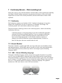
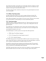
Figure 4.2.1 Model-Based Testing in the testing process
As you can see in this illustrative picture model-based testing (the box) is a functional testing
technique and it is applicable to all levels of SUT testing. Model-based testing is a black-box
testing technique for automation of tests. Normal black-box testing implies that you
manually write the needed test cases based on the requirements specification and execute
them manually. The difference with model-based testing is that you construct an abstract
behavioral model of the SUT and from that model automatically generates test cases.
There are four different categories of model-based testing:
1. Generation of test input data from domain model
2. Generation of test cases from an environment model
3. Generation of test script from abstract tests
10
4. Generation of test cases with oracles from a behavior model
The first category of model-based testing is when you generate test input data from the
domain model and you use smart selection and combinatorial algorithms so that you don’t
need to test the SUT with all combinations of input data but rather a minimal subset of the
input data. This type of generation has it benefits, you get a good set of input data but you
don’t know whether or not a test has passed of failed.
The second approach with generation of test cases from an environment model is a bit
different. The environmental model has information about statistics of the SUT environment;
operation frequencies, data values distributions, etc. From this type of model it is possible to
generate a sequence of calls to the SUT, but it is not possible to know if a test passed of
failed because the sequence does not specify the expected output.
In the third type of model-based testing you don’t provide a model but instead you provide
abstract test descriptions, which can be Unified Markup Language (UML) sequence diagram
or in some other type. With this approach the model focus on transforming these abstract
sequences to more low-level test scripts that can be executed on the SUT. The model has
information about the structure and API of the SUT.
The last approach generates executable test cases with input values and also includes oracle
information for each test case. This method makes it therefore possible to totally automate
the test case generation phase and the test execution phase. The model is a behavioral model
of the system under test, behavioral model means that the model behaves like the SUT but
the implementations is not totally accurate. The opposite of behavioral is structural and this
is what is implemented in the SUT. This category of model-based testing is more
sophisticated and complex than the other categories, but it has greater potential payback
features. Most of the commercial tools that are available on the market implements feature
from this approach.
4.3 The Model-Based Testing process
All testing processes involving functional testing needs to fulfill these four key features:
Designing the test cases: The requirements on the system must be analyzed so that the
proper test cases can be created that test all requirements. Also test criteria for passing or
failing a test must be addressed.
Executing the tests: The constructed test cases are executed on the system under test.
Analyzing the result: For each test case the system will produce an output. This output will
be compared with the criteria from the design phase. A pass or fail will be the result on each
test case.
Verifying how the tests cover the requirements: To assure the quality of the test process
and the quality of the product the coverage must be measured. This can be done using a
traceability matrix that lists each test case and which requirement it tests.
11
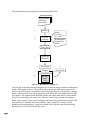
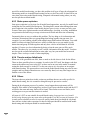
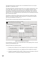
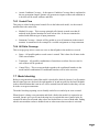
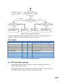
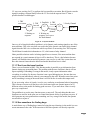
The general model-based testing flow can be illustrated like this:
Requirements
and other
documents
1.
Model
2.
Test Case
Generator
Model
Coverage
Requirements
Traceability
Matrix
Test Cases
3.
Test Script
Generator
Test Scripts
5.
Adaptor
Test Result
Test execution tool
4.
System
Under
Test
Figure 4.3.1 Model-Based Testing process
The first step in the model-based testing process is to write or design an abstract (behavioral)
model of the system under test. This model is based on the specified requirements on the
system. One difficult task is to build the model in the right detail level. It must have enough
details so that good test cases can be generated but if the model is too detailed then it will be
too complex. The abstract model should be smaller and simpler then the SUT and it should
only focus on the things you want to test. There are various ways to produce the abstract
model, some tools uses some textural language other uses some graphical notation like UML
state machines or extended finite state machines. There can also be a mixture of both
graphical and textural notation. A good tool should also be able do some model checking
that analyzes to see if the model has any errors.
12
The second step is the generation of abstract test cases from the model. In this step the tool
may need some guidance because there are almost an infinite number of different possible
test cases. The guidance can be performed in different ways in different tools. Possible
guidance criterion is which type of model coverage that should be used; all-states, alltransitions etc. Other possible guidance could be provided using use cases, all depending on
the test generation tool.
A mature model-based testing tools should also provide reports on which requirements that a
given test case tested and how much of the model that has been covered by the test suite. The
requirements traceability matrix is a table with all test cases on one axis and all requirements
on the other axis. If a test case covers a specific requirement then a mark is placed where the
test case and requirement crosses each other in the table. The coverage report indicates
which part of the model that has been tested or not tested. If some part of the model has not
been tested then it may indicate that the model has some fault, perhaps this part of the model
is statistical unreachable or the generation tool may need some more guidance to reach this
region.
The generated test cases in the second step need to be changed or transformed into test cases
that can be executed on the SUT. This is because the model is an abstract model (simplified)
and does not have all the structural features that the SUT has.
The third step takes the abstract test cases and makes them testable on the real system. This
step involves creating (or using existing) adapters that wrap around the SUT and transforms
each abstract instruction into executable instructions. The main advantage of having two
separate layers is that the abstract tests are not dependent on a specific test environment. If
the test needs to be executed in a different environment then the only change that is needed
is to change the adapter code.
The fourth step is the execution phase. The execution is done on the SUT itself or an
accurate SUT simulator. This step is always performed regardless of which type of testing
method that is used.
The fifth step is where the output of the tests is analyzed. Even this step is a normal step for
all type of testing techniques. Each test that reports a failure needs to be examined so that the
fault is located. In a manual test process the fault is often caused either by the test case or the
SUT or badly written requirements. When the MBT process is used then the area of where
the fault may be located is increased. It can be in the model or it can be in the adapter code.
4.4 Benefits with Model-Based Testing
If you asked someone what the benefits with model-based testing is almost everyone would
say that the automatic generation of test cases is the main benefit. This is absolutely true, but
MBT gives much more to the testing process.
4.4.1 Comprehensive tests
The test case generation tool traverse the model in a very thorough way and this implies that
the many test cases that are hard to come up with using manually testing can be created with
13
MBT. Model-based testing tools often have features so that it tries to test boundary values,
where statistically many faults often occur.
4.4.2 Time reduction
Testing with the model-based testing approach can lead to time reduction if the time to write
and maintain the model when generating the test cases is smaller than the time for manually
creating the test cases and maintaining them. Introducing a new method into the organization
takes time and this has to be taken into account when measuring time.
4.4.3 Finding requirement defects
In the first step of the model-based testing process the behavioral model is produced. This
model makes it possible to find omissions, contradictions and unclear requirements. If
something is unclear when making the model then it must be address and clarified to make
the work proceed with building the model. The model is built in an early stage and therefore
the requirements are examined in an early stage. Model-based testing also helps finding
undiscovered requirements that has not been put into a requirement yet.
Finding a faulty requirement in an early development phase is a very good thing, it is time
saving and cost saving and also makes it possible to design a better system. You don’t have
to do patch fixing in the end of the project.
One long-term effect of model-based testing might be to change the roll of the testers.
Instead of catching errors in the end of the project they catch them in an early phase.
4.4.4 Requirements evolution
As the project is proceeding the requirements may change. If manual testing is used then all
the created test cases must be analyzed and verified. When the requirements change it can
affect the test cases. In model-based testing on the other hand the only change needed is the
change of the model and then regenerating the automatic test case generation. Since the
model is often much smaller than the test suite than this process is less time consuming.
4.4.5 Requirement validation
A model serves as a unifying point of reference that all teams and individuals involved in the
development process can share, reuse and benefit from. The model could be of use for others
than just the testers. Maybe designers and testers should collaborate when the model is
produced. A picture (model) says more than a thousand words, is an old saying. This is true
with models too. People tend to find it easier to understand things if there are picturized.
4.4.6 Traceability
Traceability means that it is possible to relate a requirement to the model and a certain test
case to the model and the requirement specification. The traceability helps when you should
justify why a specific test case was generated from the model and what requirements have
been tested. It also helps when the model evolves and grows in size, because it enables
tracing for new test cases that belong to the new feature or modification added.
14
Requirements
Reqs-Model
Traceability
Model-Tests
Traceability
Model
Reqs-Tests
Traceability
Tests
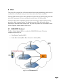
Figure 4.4.1 Traceability
There are three different types of traceability as seen in the picture; Req-Model traceability is
used to analyze which requirements are not yet in the model or how does a requirement
influence the model. Model-Tests traceability is used to visualize a given test case as a
sequence of transitions in the model or showing which transitions in the model that have not
been covered by any test case. To perform this trace the tool needs to record each transition
it takes and in which order. The last traceability aspect is Req-Test traceability and this
shows how a given requirement is tested in a given test case. This trace is the least technical
approach and it can be used either by the test engineer or by some nontechnical person. It
identifies requirements that have not been tested and show all tests that relate to a given
requirement.
4.5 Drawbacks with Model-Based Testing
Nothing comes for free. There is no such thing as a free lunch, you always pay it in some
way. Model-based testing is no exception in this matter. Skills, time and other resources
need to be allocated for making preparations, overcoming common difficulties and working
around the major drawbacks. Model-based testing is not suitable for everyone and every
development process, there are no silver bullets or “complete” testing methods.
4.5.1 Testing skills
Model-based testing demands certain skills of the testers. They need to be familiar with or
able to adapt to the model based thinking and its underlying supporting mathematics and
theories. For example if the models are made with finite state machines then the tester needs
to know how to produce such a model with its formal language, automata theory and perhaps
some graph theory. Testers also need to have knowledge about model-based tools, scripts
and programming language necessary to complete the task.
4.5.2 Splitting and merging models
In development project with more than two persons, it is often needed to split the
development task into more than one piece. Otherwise you will not use your appointed
resources in an efficient way. Splitting and merging is something that you need to do in
almost every divide and conquer development processes. This is not something that is
15
special for model-based testing, you have this problem in all type of larger development but
when using models as in model-based testing you have to do it here also. So that will be one
extra time when using model-based testing, compared with manual testing where you only
need to split the structural model.
4.5.3 State space explosion
State space explosion is a big issue for all model based approaches, not only for model-based
testing but also for model-based design etc. The thing that is meant when talking about state
space explosion is the problem when models begin to grow in size, or more precisely grow
in states. State space explosion makes model maintenance, checking, reviewing, nonrandom
test generation and achieving coverage criteria more difficult and more time consuming.
Fortunately there are ways to address this problem. The key thing to do is abstraction and
exclusion. Abstraction is that you group things that belong together into one state. For
example if you are building a model with multiple input fields and an OK button. You could
model it so that each input field can have valid or invalid data or you can model it with
abstraction and group all fields together and only have valid or invalid data for all fields
together. Of course you lose information by doing so but the state space will be much
smaller. The other way is to simply cut off, exclude, information from the model. You then
need to test the excluded information in some other way, but your model has been made
simpler. There is always a trade of when simplifying.
4.5.4 Time to analyze failed tests
When one of the generated tests fails, then we need to decide where to look for the failure.
There are three possible places to examine. It can be in the SUT itself, the adaptor code that
connects the abstract test case to the SUT or there can be an error in the model. In manual
testing the fault can only be in the SUT or the test script so it is less places to investigate
with manual testing. The generated test case from the model-based testing may also be more
complex and less intuitive than then test case created by hand, so it may take longer time to
find the cause of the failure.
4.5.5 Others
The issues that are pointed out in this section are problems that are not really specific for
model-based testing, but it is essential to bring them up for preventive reasons.
During the development process of a product, it may happen that requirements will be
changed. If the model is built using these outdated requirements then the model and the SUT
will not be the same and many faults will be found. These faults are not real faults, and a
working process to prevent this situation is needed.
All parts of a SUT are not suitable for model-based testing. Inappropriate use of modelbased testing does not give any extra value to the product, it is only a waste of resources. If it
is much easier to build test cases for a specific part by hand, then you should do it by hand.
One risk here is that it takes experience to know which part should be modeled with modelbased testing and which part should be tested manually.
16
5 Constructing a model
The most important step in modeling is to select the right abstraction level of the model. The
model needs to be accurate so that interesting test cases can be generated but it should not be
as accurate as the SUT itself. If it is to precise then it will take too much effort to produce the
model, the test generation step will be time consuming or taking infinite time and the test
cases generated may not be the one that was expected or wanted. It is a good chance that the
generated test cases will be on the wrong detail level.
To choose the right abstract level of a model is a very challenging task it will need practical
experience as many other things in life.
5.1 Model guidelines
•
Try to separate different types of functionality to different subsystems, rather than
building the entire model in just one huge and complex model.
•
Test each subsystem independently if it is possible before merging it into the full
scale model. This will help when finding smaller errors in the model.
•
Only include features, operations and data fields that you really need to meet the test
objectives.
•
Focus on the behavioral of the SUT, not the test cases that you want to produce. If
you focus on the test cases you will only be able to generate these test cases with the
tool, you may miss some interesting test cases that the tool would have found if the
focus had been on the SUT. It is the tester’s task to design the behavioral model of
the SUT and the generation tool is responsible for finding interesting test cases. Not
the other way around.
•
Try to simplify complex operations with simpler structures like enumeration of the
possible values.
•
Consider the interface, with input and output parameters, of the model in a very early
stage of the development phase. The interface detail level indicates the abstraction
level of the model.
•
Build the model in an iterative way. Don’t address all problems at once. Add
functionality and test it to insure its correctness.
•
Let other testers view and examine your model.
Selection input and output parameters are essential when building the model. If an input
parameter changes some operation in the SUT and you want to test this change, then this
input parameter should be in your model. Otherwise it is better to omit this input parameter
to decrease the complexity. Using less input parameters will probably help the generation
17
tool to generate good test cases, and also making the generation time smaller. This is because
when using a smaller amount of input parameters then the combinatorial problem in
selecting input values will be easier for the test case generation tool.
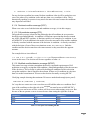
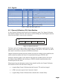
5.2 Different model notations
There are a lot of different notations in how you can model your system. Different modeling
tools use different notations and these notations have varying functionality. Some of the
groups of notation that exist will be described here.
5.2.1 Data-flow notations
Data-flow notations focus on the how data are moved around the SUT. How the data are
transformed from one type to another and how it is stored. A typical data-flow notation is the
block diagram notation in Matlab Simulink.
5.2.2 Functional notations
These notations describe the system as a set of mathematical functions. There are two
different approaches algebraic specification and higher-order functions. In the algebraic
approach functions are grouped by object types that appear in their domain. Then desired
properties are specified as conditional equations that capture the functionality. This approach
is hard to use because it quickly gets very complicated, so it is not used so much in MBT. In
the other approach, higher-order functions, the functions are grouped into logical theories.
These theories contain axioms defining the various functions and variable declarations. One
model-based tool that uses functional notation with higher-order functions is UPPAAL.
UPPAAL is collaboration between Uppsala University and Aalborg University and it is an
environment for modeling, simulation and verification of real-time system with critical time
constraints.
5.2.3 History-based notations
The principle here is to describe the allowable traces or paths of the modeled systems over
time. The notation of time is important and can be described in various ways. Time can be
linear or branching. Time structures can be discrete or continuous. The properties may refer
to time points, time intervals or both.
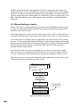
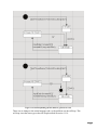
Message sequence charts (MSC) is a graphical and textual language for the description and
specification of the interactions between system components. The main area of application
for MSC is as an overview specification of the communication behavior of real-time systems.
It is good for visually showing interactions among components, but not so good at specifying
the detailed behavior of each component. Therefore it is sometimes used for showing the
generated test cases from a model-based testing tool. MSC exist in UML as well but is called
sequence diagrams in UML.
18
:web-browser
:server
:db
readTheNews
requestNewsPage
requestNews
news
newsPage
Figure 5.2.1 Message sequence chart (MSC)
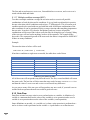
5.2.4 Operational notations
This type of notation describes the system as a collection of processes that can be executing
in parallel. The notation is particularly suited to describing distributed systems and
communications protocol.
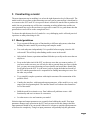
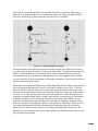
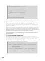
Petri net is one of the available notations in this group, it was invented by Carl Adam Petri in
1962. A Petri net consists of places (unfilled circles), transitions (filled rectangles) and
directed arcs and tokens (filled circles). Each place can hold a number of tokens and when a
token moves from a place to another place it travels through a transition and executes the
process or operation that belong to that transition. A movement of one or more tokens is
called a firing.
Firing
Transition
Token
Place
Figure 5.2.2 Petri net
5.2.5 State-based (pre/post) notations
Instead of describing what happens at a specific time, as in history-based notations, statebased notations describes the allowable states in a system at some point of time. The system
is modeled with a collection of variables, which represent the internal states of the system
plus some operations that modify these variables. Objects in an object oriented language
have much in common with these variables. Some state-based or pre/post notations are the
UML Object Constraint Language (OCL), Java Modeling Language, Z or B abstract
machine notation.
19
State-based notations are also called pre/post notations. The precondition specifies what type
of input data that is valid and constraints on them. The post condition handles the data
manipulation, which is an abstraction of how it is changed in the SUT.
Pre/post Coffee machine example with the B notation:
MACHINE
CoffeeMachine
// Name of the machine
VARIABLES
balance, limit
// Variables
INVARIANT
limit : INT & balance : INT &
// Constraints on the variables
0 <= balance & balance <= limit
INITITALISATION
balance := 0 || limit := 10
// Initial values
OPERATIONS
reject <-- insertCoin(coin) =
PRE coin : { 1, 5, 10 }
// PRECONDITION
THEN
IF coin + balance <= limit
THEN
balance := balance + coin ||
reject := 0
ELSE
reject := coin
END
END;
money <-- returnButton =
money := balance || balance := 0
END
The operations part of the code is where the real action takes place. reject <-insertCoin(coin) says that coin is an input parameter to the function insertCoin and reject is
the output parameter. Coin can only be 1, 5 or 10 which is specified in the precondition. The
rest of the lines in the function belong to the post condition. The money := balance ||
balance := 0 says that these two statements will be executed in parallel (concurrent). The
variable money will have the value of balance and balance will be set to zero, but money will
not be zero it will have the value before balance was set to zero. This can be confusing at
first if you are only familiar with sequential programming.
5.2.6 Statistical notations
These notations model a system by a probabilistic model of the events and input values. The
use of Markov chains is one model that is often used. If a model has the Markov chain
properties then many statistical features are easily received from the model. The main
property that must be fulfilled is that the next state in the model is not depending on any
previous states. The model should not remember previous steps when deciding the next step.
Statistical notations are good for specifying distributions of events and driving the choice of
test sequences and inputs for the SUT but are generally weak at predicting the expected
output, so it is not usually possible to automatically generate oracle information during test
case generation.
20
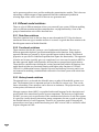
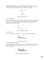
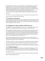
5.2.7 Transition-based notations
This type of notation describes the system as a state machine with actions performed when it
takes a transition from one state to another. Typically, they are graphical node-and-arc
notations, such as a Finite State Machine (FSM). The properties of interest are specified by a
set of transition functions in the state machine. These functions specify when a transition
should be triggered, what properties must be fulfilled to take the transition and what action
should be performed when the transition is taken.
Transition-based notations don’t have to be in graphical form, they can be in textural or
tabular form as well. But the graphical notations are more often used and some of them are
UML State Machines, STATEMATE, state charts and Simulink Stateflow charts.
C
A
S1
S2
E
S3
D
Figure 5.2.3 Simple finite state machine
21
22
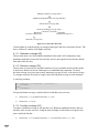
6 Test case generation
This chapter will describe which opportunities you have in controlling the automated test
case generation. It is your model-based testing tool that generates the test cases but you have
the possibility to guide the tool by selection which type of criteria the generation should use.
Different tools have different test selection criteria and often only a subset of all criteria’s
that will be presented in this chapter.
It is good to remember that MBT is a black-box testing technique and that the coverage
criteria represented here will only measure how well the generated test suite covers the
model. It is not possible to measure source code coverage of the SUT or coverage
measurements made on the SUT. This does not necessary have to be a negative thing though,
it gives the opportunity to start generating test cases using some test criteria before the actual
coding of the SUT has begun.
The real measurement of statement and branch coverage can be done when the SUT is
executed with the generated test cases.
The choice of coverage criteria determines which type of algorithms that will be used by the
model-based testing tool for generating the tests, how large the test suite will be, how long
time it will take to generate them and which parts of the model that will be tested. When
applying a coverage criterion you are saying to the tool “please try and generate a test suite
that fulfills this criterion”. Maybe you are requesting for something that is very hard or even
impossible to solve. The tool will not perform any black magic for you, it is working in a
restricted domain and will do its best in accomplishing your request. A point of failing can
be that some part of the model is statistical unreachable and therefore it is not possible to
accomplish the criteria. There is also a possibility that the tool is not powerful enough to find
a path in the model so that the criteria can be achieved to 100 percent coverage. In the case
of failing criteria the tool should be able to generate some type of report that indicates which
part that could not be covered so that it can be investigated more thorough.
6.1 Structural model coverage criteria
Structural model coverage has some similarities with code based coverage criteria that can
be used in white-box testing. The similarities are the control-flow and the data-flow coverage
criteria, but there is more that belongs to the structural model coverage genre like transitionbased and UML-based coverage criteria.
6.1.1 Control-flow
Control-flow coverage covers criteria as statements, branches, loops and paths in the model
code. The picture below shows the different categories of control-flow coverage criteria that
will be represented here.
23
Multiple Condition Coverage (MCC)
Modified Condition/Decision Coverage (MC/DC)
Full Predicate Coverage (FPC)
Decision/Condition Coverage (D/CC)
Decision Coverage (DC)
Condition Coverage (CC)
Statement Coverage (SC)
Figure 6.1.1 Control-flow hierarchy
Criteria higher up in the hierarchy are stronger and acquire the lower criterion to be true. The
lower criterion is a subset of the higher criterion.
6.1.1.1 Statement coverage (SC)
The test suite must cover all reachable statements in the model. All if-statements, loopstatements should be executed at least one time, but it is not required to test the true and the
false path of the decision.
6.1.1.2 Decision coverage (DC)
The test suite executes all true and false branches of every reachable decision in the model.
A decision or branch can be an if-statement or a conditional loop-statement. To satisfy
decision coverage a test suite must satisfy statement coverage as well, so decision coverage
is a stronger criterion. Decision coverage is also called branch coverage in some literature.
A clarifying example:
if (condition1 && (condition2 || function1()))
statement1;
else
statement2;
100 percent branch coverage could be achieved with these two test cases:
•
condition1 == true
•
condition1 == false
and condition2
== true
6.1.1.3 Condition coverage (CC)
To achieve condition coverage at 100 percent every Boolean condition must have the true
and false value in some test case. Using the same example as in decision coverage the test
suite could look like this:
•
24
condition1 == true
and condition2
== true
and function1()
== true
•
condition1 == false
and condition2
== false
and function1()
== false
For any decision regardless how many Boolean conditions it has it will be needed two test
cases. One when every condition is true and one when every condition is false. This is
theoretically speaking, in practice it may need a lot more test cases because the conditions
may depend on each other.
6.1.1.4 Decision/condition coverage (D/CC)
When a test suite covers both decision and condition coverage, it is in this category.
6.1.1.5 Full predicate coverage (FPC)
Full prediction coverage is based on the philosophy that all conditions in an expression
should be tested independently. A condition is a Boolean expression that does not contain
any AND, OR and NOT operators. A Boolean variable is an example of a condition. A test
set fulfills FPC if each condition in the model is forced to true and to false and the condition
is directly correlated with the outcome of the decision. A condition c is directly correlated
with the decision d if one of these two situations occurs, dÙc or dÙnot(c). Both the
condition and the decision must have the same outcome or they must have the opposite
outcome.
For example this set is not allowed.
and c == false Æ d == true. Because neither dÙc nor dÙnot(c)
is true in this cause. The decision will be true regardless of what c is.
c == true Æ d == true
6.1.1.6 Modified condition/decision coverage (MC/DC)
This control coverage criterion strengthens the directly correlated requirements of full
prediction coverage by saying that each condition c should independently affect the outcome
of the decision d. This coverage is achieved by holding all conditions fixed in a decision
except the condition c that is tested for the moment. If there are N conditions in a decision
then it is needed a maximum of 2N tests on the decision for totally covering MC/DC.
Clarifying example showing that maximum 2N tests are needed and enough (not a proof):
condition1 && (condition2 || condition3)
Let’s say that we want to test condition1 then we will hold the other two conditions fixed
(one of the conditions on the right side of the && operator must be true to fulfill MC/DC).
The condition1 can be true or false, so there will be two tests when testing condition1. But
because of the && operator condition1 must be true when testing the right side of the &&.
Condition1
Condition2
Condition3
true
false
true
true
true
true
false
false
false
false
false
true
Table 6.1.1 Test pattern for fulfilling MC/DC
25
The first and second tests test condition1, first and third test condtion2, and condition3 is
tested with the third and fourth.
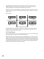
6.1.1.7 Multiple condition coverage (MCC)
To achieve multiple condition coverage the test suite needs to exercise all possible
combinations of each decision and its conditions. It is very hard to perform this in practice
because a decision with N conditions needs to have 2N different tests. This is because each
condition needs to be tested with true and with false with all different combinations of the
other conditions. It can be questioned if this coverage criterion adds something important to
the test suite. It can do it if it is hard to find distinct good test, because all possible
combinations will be tested. But is there really the time for doing this type of testing? Many
of the test cases will not lead to anything, because of the operators. The example below
shows this. The exponential growth of the tests need also makes it impossible to fulfill MCC
if there are many conditions.
Example:
The same decision as before will be used.
condition1 && (condition2 || condition3)
It has three conditions so eight tests are needed, the table show each of them.
Condition1
Condition2
Condition3
true
true
true
true
false
false
false
false
true
true
false
false
true
true
false
false
true
false
true
false
true
false
true
false
Table 6.1.2 Test pattern for MCC
All of these tests will not produce any different result. The first, second and third will return
the same result. The last four will also return the same result, because condition1 == false
and then the value of condition2 and condition3 will not do any difference.
As you can see many of the test cases will not produce any new result, if your task is not to
test the Boolean operators then all tests could be good test cases.
6.1.2 Data-Flow
Data-flow-oriented coverage criteria cover read and writes to variables. A definition of a
variable is a statement that sets the value of the variable (a write operation) and a use of a
variable is an expression that uses the value of the variable (a read operation).
Some definitions are needed, v is a variable, Dv is when a write operation is performed on v
and Uv is when a read is performed on the variable v. A path from Dv to Uv that does not
26
contain any other definitions on v is called def-use pair and is denoted (Dv, Uv). This
definition ensures that the variable v has not been changed when it is read by Uv. A def-use
pair is feasible if there is a test path from Dv to Uv, otherwise it is infeasible.
All-definition-use-paths
All-uses
All-definitions
Figure 6.1.2 Data-flow hierarchy
6.1.2.1 All-definitions
This is the weakest data-flow coverage. It requires that the test suite tests at least one def-use
pair (Dv, Uv) for every definition Dv. One path is enough. Easier said all write operations
should have read operation and when the read is performed the value should not have
changed from when the write was done.
Dv1b
Dv1a
Uv1a
Uv1b
Uv1c
Uv1d
Figure 6.1.3 All-definitions example
6.1.2.2 All-uses
This coverage extends the all-definitions. Now all uses of a variable should be tested.
Dv1b
Dv1a
Uv1a
Uv1b
Uv1c
Uv1d
Figure 6.1.4 All-uses example
6.1.2.3 All-definition-use-paths
This is the strongest coverage of data-flow coverage. All feasible paths from all Dv to all Uv
should be tested. This coverage usually requires too many test cases because there will be
too many combinations.
Dv1b
Dv1a
Uv1a
Uv1b
Uv1c
Uv1d
Figure 6.1.5 All-definition-use-paths example
27
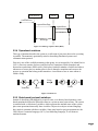
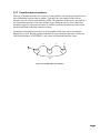
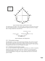
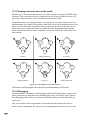
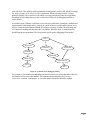
6.1.3 Transition-Based
In this section the most common model-based testing coverage for transition-based coverage
will be presented and it will be explained how they relate to each other. Transition-based
models are built using states and transitions, in some notations like state charts it is possible
to have hierarchies with states, so th
thaatt one state can hold other states inside itself.
models
To exemplify transition coverage criteria two m
odels will be used. One is a state chart and
one is a normal finite state machine (FSM).
S
S1
S4
S6
C
S5
S2
S7
D
B
A
E
S3
S8
Figure 6.1.6 State chart
For a state chart there is something called configuration. A configuration is a snapshot of the
state chart at some time. The configuration tells in which states the model is currently in.
Because there can be parallelism and hierarchies in the state chart the configuration is made
by enumerating all states it is in for that moment. It can for example be when the state chart
is in the state {S, S1, S2, S4, S6, S8} and if the D transition is taken the configuration will
change to {S, S1, S2, S4, S5} instead.
A
S1
C
S2
B
E
S3
D
F
Figure 6.1.7 Finite state machine
28
G
S4
If the below transitions-based coverage are applied to models with state variables and guards
on the transition then it is usual to restrict the allowed paths to only paths that are reachable.
This is because you don’t want the coverage measurement to measure paths that are
impossible to reach.
All-paths
All-transition-pairs
All-loop-free-paths
All-configurations
All-round-trips
All-transitions
All-one-loop-paths
All-states
Figure 6.1.8 Transition hierarchy
6.1.3.1 All-states coverage
This coverage ensures that all states in a model have been visited at least once. To cover allstates in the FSM in Figure 6.1.7 a possible path can be B;D;G and to cover it in the state
chart in Figure 6.1.6 these transitions A;C;E would be enough. This is because it will start in
S2 (and S1) and S5 (and S4) simultaneously. By taking the A transition state S3 will be
covered and when C is taken then S7 (and S6) is reached. The last transition E covers state
S8 and now all states are covered.
6.1.3.2 All-configurations coverage
In this coverage measurement all configurations in the model must be covered at least once.
If the model does not have any parallelism then this coverage criteria is the same as all-states
coverage.
For the state chart Figure 6.1.6 this coverage can be achieved by traversing the model in this
order C;E;A;D;C. There are 6 possible configurations because. It is calculated by
multiplying the number of states in each parallel state machine. Only the inner states are
counted. The left state machine has two inner states, namely {S2, S3} and the right has three
{S5, S7, S8}. So the possible configurations are 2*3=6.
6.1.3.3 All-transitions coverage
In all-transition coverage the thing of interest is not states as in the two previous coverage
criteria but instead transitions. As the name indicates all transitions in the model must be
taken at least once.
To achieve this in the FSM model in Figure 6.1.7 these two traversations are possible
A;C;E;G and B;D;F.
29
To achieve the same thing with the state chart in Figure 6.1.6 is ambiguous. It depends on
how the interpretation is done. There is no real “right” interpretation of the D transition. Is it
enough only to take the D transition from one of S7 or S8 or should the D transition be like
two transitions one from S7 and one from S8? Different tools interpret it differently and you
need to find out which interpretation is used.
6.1.3.4 All-transition-pairs coverage
The all-transition-pairs coverage says that all incoming transitions must be tested together
with all outgoing transitions in a state. For example in state S3 in Figure 6.1.7 there are two
incoming and three outgoing so there will be six (2*3=6) combinations, namely C;E, C;F,
C;G, D;E, D;F and D;G.
6.1.3.5 All-loop-free-paths coverage
This coverage criterion ensures that all loop free paths are covered. A loop free path is a path
that does not contain repetition of any configuration. The FSM model in Figure 6.1.7 has
four different configurations, one for each state. To achieve all-loop-free-paths these tests are
needed A;C;G, A;D;G, B;C,G and B;D;G. Transition E and F can’t be taken because this
would result in a configuration state that has already been reached because it is a loop back
to a previous state.
It is possible that some states in the model will not be reached when using all-loop-free-paths,
for example if the F transition leads to a state, say S5, and then a transition H leads back to
state S3. Then the state S5 nor transition H would be reached or walked.
A
S1
C
S2
E
G
S3
S4
H
B
D
F
S5
Figure 6.1.9 All-loop-free-paths example
6.1.3.6 All-one-loop-paths coverage
The all-one-loop-paths coverage is fulfilled when all loop-free paths have been taken and all
paths that loop once. A more precise definition is, every path contains at most two
repetitions of one (and only one) configuration.
For the FSM in Figure 6.1.7 the required test paths will be a combinations of A,B,C,D as in
all-loop-free-paths. In state S3 it will take either E or F or none of them before taking G. For
example A;D;E;G or A;D;G.
30
6.1.3.7 All-round-trips coverage
This coverage criterion is similar to all-one-loop-paths in some sense. It requires that all
loops are tested in the model, but it is weaker because it only requires one path for testing the
loop. In all-one-loop-paths it is required that all paths for a loop are covered. By having the
all-round-trips in this way it is much easier to accomplish this criterion in practice. Because
it will be a linear among of test cases needed.
For testing the FSM model in Figure 6.1.7 with all-round-trips coverage it is only required to
test it with these two test paths A;C;E;G and B;D;F. All loops have been visited and all
transitions have been taken. So the criteria are fulfilled.
6.1.3.8 All-paths coverage
All possible paths must be covered in all-paths coverage. In the FSM model in Figure 6.1.7 it
will be an infinite number of test paths, because it is possible to loop forever on the E or F
when you are in state S3. This criterion is only suited for small models without any loops or
with some boundary on how many loops to cover.
6.1.4 UML-Based
The UML language is for specifying, visualizing, constructing and documenting the artifacts
of the software system. UML provides a variety of diagrams that can be used to present
different views of an object oriented (OO) system at different stages of the development life
cycle. A lot of the coverage criteria that has been presented in previous sections of this
chapter are also suitable for UML-based coverage criteria, for example decision and
transition coverage can be used on UML state machines.
Only new coverage criteria that have not been mentioned in earlier sections will be described
here.
6.1.4.1 Class Diagram
A class diagram shows the static structure of a system. It identifies all the entities, along with
their attributes and how the entities in the system relate to each other. These relationships or
associations are represented by links among the entities. The links can have ranges specified
on each end. For example if a link has 1 on one of the ends and 5 on the other, then it means
that the entity with 1 can have 5 entities of the other type.
6.1.4.1.1 Association-end multiplicity (AEM) coverage
This coverage method is fulfilled if and only if it exist a test case that causes each
representative multiplicity-pair to be created.
Example:
There exist a class A and a class B. There is an association between A and B. The range on
the A side is 1..1, meaning that B can only have one instance of A. On the B side of the
association there is a range of 0..5, meaning that A can have 0 to 5 instances of B.
One strategy to get the multiplicity-pair is to partition the equivalence into groups and doing
so for each class. Class A only has one equivalence class, namely {1}. Class B has three
31
equivalence classes {0}, 1..4 and {5}. The combination of the all equivalence classes of A
and B will give the multiplicity-pairs: (1,0), (1,2) and (1,5). In the second pair the 2 could be
1, 2, 3 or 4 it does not matter.
6.1.4.1.2 Generalization (GN) coverage
Generalization is typically implemented as inheritance. Inheritance is one of the main
features of an object oriented language. One class can be the parent (generalization) to some
other classes which are children (specializations). E.g. the parent class is Vehicle and a child
to this parent could be Car, Motorcycle or Bike. To be able to cover this coverage criterion it
is needed that all specializations in all generalizations are created at least once.
6.1.4.1.3 Class attribute (CA) coverage
This coverage criterion assures that a set of possible values for each attribute in a class is
tested, all combinations of these values should be tested. The possible values can be all
combinations of valid attribute values or a subset of them. If it is a subset then some good
selection method is needed for selecting a good partition of attribute values.
6.2 Data coverage criteria
The valid input range of data to a system is often very large, and even if it is not so large
then it quickly leads to a combinatorial explosion if all combinations of values should be
tested. Data coverage criteria are useful for selecting a good set of few data values to use as
input to the system.
Let’s image that we have this easy example:
x:
y:
0..99
0..19
Condition: x > 50 and y > 10
Figure 6.2.1 Easy data coverage example
Without any data coverage criteria then all combinations need to be tested. The number of
combinations will be 100*20 = 2000 different test cases. Is this really needed?
6.2.1 Boundary value testing
The idea with boundary value testing is straightforward, it is often more likely to find a fault
near a boundary then if you just select some value in the range. E.g. x values in Figure 6.2.1
from 0 to 49 (50) belongs to the same equivalence group so there is really no need to test
more than one of the values in this region.
This integer example will be used to illustrate the boundary value testing coverage’s.
32
y
2
2
x +y ≤ 25
x+y≤5
-x + y ≤ 5
(0,5)
(-2,3)
(3,2)
(5,0)
(-5,0)
(-4,-3)
x
(4,-3)
(-3,-4)
(3,-4)
(0,-5)
Figure 6.2.2 Integer example of boundary points of a shape
Four different type of boundary value testing will be presented, the hierarchy between them
are as the picture below shows. A coverage method that is higher up in the tree is stronger
than a coverage method lower done in the tree.
All-boundaries Coverage
All-edges Coverage
Multidimensional-boundaries Coverage
One-boundary Coverage
Figure 6.2.3 Boundary value testing hierarchy
6.2.1.1 All-boundaries coverage
The all-boundaries coverage criterion is the strongest boundary value criterion. It acquires
that all boundary value point is tested. This is often not realistic in a larger system where
there are many conditions and with complex boundaries. But in Figure 6.2.2 this would not
be impossible because there are only 24 boundary value points.
6.2.1.2 Multidimensional-boundaries coverage
For a test suite to satisfy this coverage method it is needed that every variable is assigned its
minimum value and maximum value at least once. In Figure 6.2.2 this can be done by
choosing the boundary value points: (-5,0), (0,5), (5,0), (0,-5). Instead of making 24 test
cases as in all-boundaries coverage, this coverage method only needs 4 test cases in this
specific example.
33
6.2.1.3 All-edges coverage
In all-edges coverage the decision is broken down to its conditions. E.g. Figure 6.2.2 have
three conditions namely x2+y2 ≤ 25, x + y ≤ 5 and -x + y ≤ 5. Each of these conditions
defines an edge in the shape. To fulfill all-edges coverage at least one boundary point from
each edge must be tested. This can be achieved with the points (0,5) and (3,-4). There are
lots of different combinations to fulfill the coverage in this example.
6.2.1.4 One-boundary coverage
This boundary coverage is the weakest criterion, it only requires that some boundary value
point is tested. Only one test case is therefore needed.
6.2.2 Statistical data coverage
All data can’t use boundary value testing, e.g. a enumerated domain of colors:
Color : {Red, Green, Blue, Yellow, Black, White}
It is not possible to use boundary value testing here because there is no order of the values,
they are not ranked. In these cases statistical data coverage method can be used instead.
6.2.2.1 Random-value coverage
This criterion requires that the values of a given data variable in the test suite follow a given
statistical distribution, e.g. uniform, Poisson or Gaussian distribution.
6.3 Requirements-based criteria
Making sure that each requirement on the system is tested is a key issue in the testing
process. The pass of all requirements ensures that the system delivers what it should.
Therefore the requirements can be used both to help in the test generation and measure the
level of coverage of the generated test cases.
There are two main approaches to achieve requirements coverage:
34
•
Insert the requirements directly to the behavior model so that the test generation tool
can ensure that they are fulfilled.
•
Use some formal expression, like logic statements that drives the test generation tool
to look for something special behavioral in the model.
6.4 Explicit test case specifications
Explicit test case specifications can be used to guide the test generation tool to examine
some certain behavior of the system. These specifications can e.g. be a use case model which
specifics some interesting path of the model that should be tested carefully.
The main advantage of these types of specifications is that they give extremely precise
control over the generated test cases. The disadvantage is that it can be very time consuming
creating these explicit test case specifications and you also lose some of the advantage with
model-based testing which is letting the automatic test generation tool provide all test cases
that are needed.
35
36
7 Conformiq Qtronic – Pilot modeling tool
In the pilot, where a part of the Base Station Controller (BSC) will be modeled, the modeling
tool Qtronic Modeler and the automatic test generation tool Qtronic will be used. In this
chapter these two tools will be shortly introduced, and the main features of them will be
explained.
7.1 Conformiq
The Conformiq company was founded in 1998. Conformiq’s headquarter is located in
Finland. The company has 10 years of experience of Automated Test Design. The
Conformiq Qtronic tool is their third evolution of their product.
The main tool that Conformiq provides is the Conformiq Qtronic, which is described by
Conformiq in this way:
Conformiq Qtronic is an ongoing attempt to provide an industrially applicable
solution to the following technical problem: Create an automatic method that
provided an object (a model) M that describes the external behavior of an
open system (begin interpreted via well-defined semantics) constructs a
strategy to test real-life black-box systems (implementations) I in order to
find out if they have the same external behavior as M.
7.2 Qtronic Modeler
The Qtronic Modeler is a lightweight UML state chart editor that comes bundled with the
main program Qtronic. This modeler makes it possible to easily create state machines that
can be used in Qtronic directly without any need of converting to Qtronic Modeling
Language (QML).
7.2.1 QML – Qtronic Modeling Language
The Qtronic Modeling Language is both a textural and a graphical notation. It is possible,
even if it is not recommended, to design the whole model using just the textural notation.
The textural notation is a superset of Java with some ideas from C#, plus some extra Qtronic
specific features. The QML language does not include the standard libraries that come with
Java or C#. This textural notation is sometimes called action language. The graphical
notation uses UML state charts to create UML state machines.
Figure 7.2.1 QML, Java and UML
37
7.2.1.1 Textural notation
The keywords in QML that do not exist in Java are listed below. QML has more differences
compared to Java, but these differences have to do with different interpretation of the
keywords. The ones listed below are the keywords that are new, regarding to what Java has.
Keyword
Meaning
after
checkpoint
Inbound
Outbound
omit
record
require
requirement
system
Defining that something will happen after some period of time.
Inserts a new checkpoint into the model, Qtronic will try and cover this.
Defines an external inbound port to the system.
Defines an external outbound port from the system.
Specifies that the record field is omitted from the record instance.
Defines a record type, only records can communicate with an environment.
Require that the expression is true.
Inserts a requirement into the model.
Defines the system block which contains the external ports.
Table 7.2.1 Difference between Java and QML
To get more information about differences between QML and Java read the Qtronic User
Manual.
7.2.1.2 Graphical notation
The graphical notation have some symbols that you build your UML state machines with,
each of them will be briefly described below.
Initial State – Each state machine need to have one and only one
starting point. This is where the execution starts.
Final State – This is a final state where the execution terminates. A
model does not have to have a final state.
Basic State – This state is a normal state. The upper part contains the
name of the state and the in the lower part some action language code
can be places that will be executed when you are in this state. The
lower part may be empty.
38
Sub State – This state has a state machine inside itself. It is used for
information hiding so that the model will be simpler to understand.
Junction – This state has similarities with the basic state but it has no
unique name and can’t contain any action language code.
Transition – This arc connects a source state with a destination state.
Each transition can have a trigger, guard and/or action. All of them are
optional. The syntax is Trigger[Guard]/Action.
A trigger specifies the pattern of data to match and receive incoming
data. The guard checks the incoming data and if the guard condition is
true than the transition fires. If the transition fires than the Action will
be performed.
7.2.2 Example
This state machine example models a file that contains a number of individuals. The
individuals are used for setting up a network with cells, saying which cells that are neighbors
with each other when configuring a Base Station Controller (BSC).
It is possible to increase the number of individuals and decrease the number of individuals.
•
When increasing the number of individuals using command SAAII in the BSC, the
BSC checks that it really is an increase and that the maximum limit is not exceeded.
•
When decreasing the number of individuals using command (SAADI) in the BSC,
the BSC checks that it is a decrease, the minimum limit is not reached and that no
individual will be removed when the decrease is done.
The file can be illustrated like this:
Occ.
Occ.
Occ.
Occ.
Free
Occ.
Free
1
2
3
4
5
6
7
Highest used individual: 6
Number of individuals: 5
Figure 7.2.2 Free individuals example
39
The implementation makes it possible to have a free individual in between two occupied
individuals, e.g. individual 5 is free.
The implementation had a fault that made the BSC to do a complete exchange failure, and a
restart. When a BSC is forced to do a restart it is seen as something really bad, it almost
never happens. The problem was that when the decrease command was used it compared
with the number of used individual and not the highest used individual. They are the same
when there are no free individuals in between, but when there are free individuals in between
they are not the same anymore.
The problem was that the tester did not come up with a manual test case that tested what
happened if you used the command SAADI, saying the new size should be five and there
were some free individuals as in Figure 7.2.2.
The model that was produced using model-based testing looked like this:
Figure 7.2.3 Free individuals state machine
It first initialized a vector with some occupied individuals in the beginning of the vector and
let the rest of the individuals be free.
From the Idle mode state it had four options:
40
•
Inserting a new relation to the vector, changed one of the free positions to occupied.
•
Removing a relation from the vector, changed one of the occupied to free instead.
•
Sending the command SAAII to the BSC, telling it to increase the number of allowed
relations in the file. This made the checking as described above.
•
Sending the command SAADI to the BSC, telling it to decrease the number of
allowed relations in the file. It performed the required checking as described above.
Another interesting feature of this model is the loopCount variable. This loop variable forces
Qtronic to do at least three operations before it can go to the final state. The test generation
program (Qtronic) which is described in the next section has an option called “Only
Finalized Runs”. When this option is used it forces Qtronic to take each generated test case
from the starting point of the model to a final state in the model. This is a good option and it
should be used whenever it is possible. If the option is not used then Qtronic will have to
decide for itself when it should end a test case, Qtronic can decide that it wants to end a test
case after it has just taken the first transition. This will obviously not be an interesting test
case, because this test case will not test anything interesting.
Qtronic was not able to find this fault using the general model that only said that it was not
allowed to decrease below an occupied individual, what Qtronic generated was a test case
that looked like the figure below.
Occ
Occ.
Occ.
Occ.
Free
Free
Free
1
2
3
4
5
6
7
Decrease to 1 individual
Occ
1
Error: Not allowed to decrease below occupied individual
Figure 7.2.4 Test case using general model
The model was changed so that it looked for one occupied individuals and then free
individuals before. This is the test case that you really wanted Qtronic to produce. Now
Qtronic were able to generate the correct test case, but now the model specifically asked for
this test case. This is not the way you should do it when you design your behavioral model.
Occ.
Occ.
Occ.
Occ.
Free
Free
Occ.
1
2
3
4
5
6
7
Decrease to 5 individual
Occ.
Occ.
Occ.
Occ.
Free
1
2
3
4
5
Error: Not allowed to decrease below occupied individual
Figure 7.2.5 Test case generated using guide model
So the conclusion of this simple example is that it is hard for the test generation tool to find
test cases that you did not expect.
41
7.3 Qtronic
When the SUT behavioral model has been produced it is time to automatically generate test
cases. This is the purpose of the Conformiq Qtronic tool. The Qtronic tool takes the
behavioral model as an input and automatically generates interesting test cases from the
model.
The behavioral model describes how the system should work from the user’s perspective.
This model does not need to reflect the real structural model, which is the implementation. It
is enough that it describes the intended behavior of the system.
Qtronic can be used in two different testing approaches. One is called online testing and the
other is called offline test generation. In online testing Qtronic and the behavioral mode is
directly connected with the system under test and in offline test generation Qtronic produces
test cases that are saved so that they can be executed in the future.
Figure 7.3.1 Qtronic overview
7.4 Online Testing
Using online testing Qtronic examines the behavioral model that is provided and it will
select interesting test cases that are executed directly on the system under test. The system
under test will report back to Qtronic what the response for the test case that is executed.
Qtronic also runs the same test case on the behavioral model. These two test runs should
produce the same result, otherwise there is some fault in the behavioral model or in the
implementation. Qtronic will get online information about each test case and will then be
able to change the next test case regarding to what information it has got.
42
To get the Qtronic and the system under test to understand each other an adapter is needed.
This is because the behavioral model and the system under test have not entirely the same
structure so some type of conversion will be needed.
The online testing procedure automates not only the test case generation phase but also the
test execution phase.
7.5 Offline Test Generation
In offline testing Qtronic produces test cases by examine the behavioral model. The
behavioral model is the only information that Qtronic has about the system under test.
In the offline mode Qtronic creates a library of test cases (assets). These test cases can later
be executed on the SUT, either manually or in a more automatically fashion.
7.5.1 Script generation
Finding test cases is a difficult combinatorial task to do. Therefore Qtronic provide some
options so that the user of Qtronic can select to a proper value to help Qtronic in the test
generation phase.
To record the test cases that Qtronic is able to find a scripter generation adapter is used.
Either this adapter is custom made for the system under test or some of the adapters that
come bundled with Qtronic can be used.
The bundled adapters are able to produce test scripts in the following formats:
•
HTML (Hyper Text Markup Language)
•
TTCN-3 (Testing and Test Control Notation version 3)
•
TCL (Tool Command Language)
The HTML adapter produces the most human readable test suite. In the report all coverage
aspect of the model is shown, it tells how many percent of the model that Qtronic was able to
cover, and shows which parts that it was unable to find a test case for.
It is possible to insert requirement statements into the behavioral model. The generated
HTML report will build a matrix with all requirements and all test cases so that it will be
easy to see which test case that fulfills which requirement.
The HTML report also shows exactly how each test case should be executed according to the
behavioral model. Each test case can be viewed in a message sequence chart (MSC).
43
7.6 Model coverage methods
Qtronic provide a number of different coverage methods for analyzing the behavioral model
and producing test cases. The tester/user will select which type of coverage Qtronic should
try to achieve.
They are grouped into four categories that view the model from different directions.
•
State charts
•
Conditional branching
•
Control flow
•
All paths
7.6.1 State Charts (State Machine)
The state charts group has four different coverage methods. These coverage methods have to
do with the graphical part of the behavioral model. The graphical part is the UML State
Machine.
•
State Coverage – All states in the UML State Machine must be visited at least one
time in the generated test suite.
•
Transition Coverage – All transitions in the UML State Machine must be taken at
least one time in the generated test suite.
•
2-Transition Coverage – This coverage principle is the same as all-transition-pair that
was described in the test case generation chapter. It is fulfilled if all transitions in to a
state are tested together with all combinations of out transitions from a state.
•
Implicit Consumption – This coverage method guides Qtronic to send signals that the
model does not handle on any outgoing transition. With this feature selected Qtronic
will send signals that the model does take care of and without this feature Qtronic
will focus on what the model really is able to handle.
7.6.2 Conditional Branching
In the conditional branching group the focus is on generating test cases that examine how
well different sides of branch can be covered.
44
•
Boundary Value Analysis – This method groups an arithmetic condition into the
minimum equivalence group and creates an input value for each equivalence group.
If the condition is x == y then the equivalence groups will be x < y, x == y, x > y.
•
Branch Coverage – Using this method all statements on the true and the false path of
a branch will be covered. It ensures that an if-statement will be true in some test case
and false in some other test case for example.
•
Atomic Condition Coverage – Is the same as Condition Coverage that is explained in
the test generation chapter. Qtronic will generate test inputs so that each condition in
a decision will be tested with true and false.
7.6.3 Control Flow
This group is related to the general control flow in the behavioral model, it is the textural
notation that is the main focus.
•
Method Coverage – This coverage principle tells Qtronic to make sure that all
methods in the textural notation are used at least once. It does not examine the
method with different type of input parameters.
•
Statement Coverage – Qtronic will be guided to cover all statements in the textural
notation. A statement can for example be a variable assignment or a loop-statement.
7.6.4 All Paths Coverage
This coverage group tries to create test cases so that all paths in the model are covered.
•
States – All possible paths to reach a state is created. This is done for all states in the
UML state machine.
•
Transitions – All possible combinations of transitions are taken. One test case for
each of them will be produced.
•
Control Flow – This coverage method respond to the conditional branches in the
model and all combinations of conditional branches will be in the test suite.
7.7 Model checking
Before a test generation is started the model is checked for faults by Qtronic. It will examine
that all signal types are declared, the right number of in and out ports are declared. Methods
in the textural notation that is not in use will be omitted from the model so that they will not
be in the coverage measurement.
The model checking reporting is user-friendly and tells were and why an error occurred.
When Qtronic is doing a test generation and finds a fault in the model it is reported as an
assertion. Qtronic gives a trace stack showing how it reached this state. Qtronic looks for
example for index out of bound when values are fetched from a vector or hash table, finding
when a state machine reaches a deadlock state or when some other assertion is activated.
45
46
8 Pilot
This pilot will investigate how efficient the model-based testing methodology can be used in
a normal flow of functional testing of a new feature in the base station controller.
First the GSM Network will be shortly introduced, followed by the manual testing procedure
at the BSC department in Ericsson and then the actual feature will be described.
The feature that will be modeled has already been tested using the normal function testing
procedure, which is manual testing. The manual test scope will be the baseline for the
measuring of the model-based testing result. The pilot will produce test cases and these tests
will be compared with the manual created tests.
8.1 GSM/GPRS Network
The Base Station System (BSS) is a node in the GSM/GPRS Network. The main
components in the BSS are:
•
Base Station Controller (BSC)
•
Radio Base Station (RBS) / Base Transceiver Station (BTS)
Figure 8.1.1 GSM/GPRS Network
47
The BSC handles most radio related functions. The BSC manages the radio network, e.g.
configuration of the network and handling of connections to Mobile Stations (MS) including
handovers. A handover can happen for example when a MS changes its position and come
closer to another Radio Base Station (RBS), also called Base Transceiver Station (BTS). The
RBS contains the antenna system, radio frequency power amplifiers, and digital signaling
equipment.
8.2 Manual testing procedure
Before a new feature is implemented and tested a document called Implement Proposal (IP)
is written. This document describes what should be implemented and what changes will be
needed in each block of the BSC.
The designer updates the current code base and performs unit test on the block that he/she is
working on. When the unit tests have passed, the updated code is given to a functional tester.
At the same time as the designer starts the update phase, the functional tester starts creating
test cases. To his assistance the functional tester has several document, Implement Proposal,
Requirement Specification (RS), Function Specification (FS), and Function Description (FD).
The function specification describes a block in the BSC and the function description
describes the block in more detail.
Before the functional tester starts executing the test cases there is an inspection meeting,
where all test cases are examined and it is decided if the test coverage is enough. If the test
coverage is sufficient then the functional tester starts the execution phase of the test cases.
When all test cases have been passed in function test the updated code is delivered to system
test that will perform performance tests on the system.
Requirements and other
documents
Creating Test Cases
Test Cases
Inspection Meeting
Test execution tool
System Under Test
Figure 8.2.1 Manual testing process
48
Test Result
8.3 The modeled feature - RTTI
This pilot will test a new feature in the BSC node.
The new feature that will be tested in the pilot is called Reduced Transmission Time Interval
(RTTI). Before the introduction of this feature the only Transmission Time Interval (TTI)
mode that existed was Basic Transmission Time Interval (BTTI).
The TTI mode decides how the data is sent over the channel from the network to the Mobile
Station (MS). A mobile station is the device nearest the user, it can for example be a cellular
phone, a computer or some other device that has a transmitter and a receiver (transceiver).
When a mobile station transmits or receives data, it is sent using one or more channels that
are using a specific spectrum of the frequency domain.
8.3.1 Basic Transmission Time Interval (BTTI)
In the basic TTI mode a transmission of a data burst is done by that the mobile station and
the base station controller first agrees on a channel to do the transmission on. The whole
transmission is sent on this channel, from the beginning to the end.
Assuming that we have 8 channels that can be used for sending data simultaneously, the
mobile station and the BSC agrees on sending on timeslot 3. The data will be sent on this
channel until the time period ends. The figure below shows this, A, B, C and D is the data
sent on this timeslot.
0
1
2
3
4
5
6
7
Timeslot number
A
B
C
D
Time period
Figure 8.3.1 BTTI timeslot example
8.3.2 Reduced Transmission Time Interval (RTTI)
The reduced transmission time interval technique makes it possible to send the same data but
using pairs of timeslots. The timeslots must be consecutive, meaning that having timeslot 3
and 4 is allowed for using RTTI but if the mobile stations have timeslots 3 and 5 than it is
not possible to use RTTI.
49
The RTTI feature reduces the time that is needed for transferring the data over the air
interface. The receiver will be able to quicker respond with its acknowledgement back to the
transmitter. The data throughput is not increased using RTTI, it is only the Round Trip Time
(RTT) that is lowered.
The mobile station can have a maximum of two RTTI pairs (four timeslots) in the downlink
direction and one pair (two timeslots) in the uplink direction. This is the maximum but it
depends on how many timeslots the mobile station can have simultaneously. If it can only
have three timeslots in the downlink direction then it only can have one RTTI pair in the
downlink direction, each pair needs two timeslots. If the mobile station can only have two
timeslots in the downlink and two timeslot in the uplink but only three timeslots
simultaneously then it can only have one RTTI pair in one of the directions.
Using the same figure that was introduced in the BTTI section, RTTI would look like this.
0
1
2
3
4
A
C
B
D
5
6
7
Timeslot number
Time period
Figure 8.3.2 RTTI timeslot example
8.4 Model delimitations
This pilot has been limited to cover only the Connection Control block and the Channel
Utilization block in the BSC and only the functions for reservation of a TBF (Temporary
Block Flow) and what happens when the BSC detects that a channel is faulty. A TBF is
something that groups the mobile station timeslots in one direction together. The mobile
station can have one uplink TBF and one downlink TBF.
8.5 Model-Based Testing process delimitations
In this pilot the whole model-based testing process will not be investigated. This is because
of the time budget and tight deadline for this pilot. In the picture below the process to the left
is the general model-based testing process and to the right is the process that has been used
in this pilot.
50
General process
Pilot process
Requirements
and other
documents
Model
Test Case
Generator
Requirements
and other
documents
Model
Coverage
Requirements
Traceability
Matrix
Test Cases
Model
Test Case
Generator
Model
Coverage
Requirements
Traceability
Matrix
Test Cases
Test Script
Generator
Expert group:
Analyze test cases
Test Scripts
Adaptor
Test Result
Test Execution Tool
System
Under
Test
Figure 8.5.1 General MBT compared with the process used in the pilot
8.6 Input documents
The input documents used for this pilot has been the Implement Proposal (IP), Function
Specification (FS) for the two modeled blocks and an introduction PowerPoint presentation
of the RTTI feature.
The Ericsson Post-it - PDU GSM RAN Knowledge Database Wiki (Internal) has also been
helpful when looking up acronyms and finding easy understood explanations of
implementations in the BSC.
51
8.7 Modeling tool
The modeling tool used in this pilot has been the Conformiq Qtronic Modeler. It provides a
lightweight framework for building models that can be directly used in Conformiq Qtronic
without any transformations in format.
8.8 Test Case Generator
The test case generator for this pilot has been the Conformiq Qtronic tool. Several of
different versions have been used during the pilot period. Starting with version 1.2.1 and
then quickly moving to 1.3.0 (alpha) and in the end of the pilot using version 1.3.1. The
stable version 1.3.1 has been used for generating the final test case results.
Qtronic can work in two different modes; Offline Script Generation and Online Testing.
Online Testing means that Qtronic is directly connected to the system under test when
generating test cases. In the Offline Script Generation mode Qtronic and the SUT are not
connected together. The test cases are run on the system at a later stage. In this pilot only
Offline Script Generation will be used.
Qtronic supports different adapters for saving the result of the test case generation step. The
adapter used in this model will be the HTML Script Generator that comes bundled with
Qtronic. This is because it provides the best visualizing of the generated test cases. The
learning threshold is also the lowest for this adapter, which is good because the persons that
will analyze the generated test result will rapidly need to understand how the test cases are
described.
8.9 Analyze generated test cases
The generated test cases from Qtronic will be analyzed by a group of test experts.
The RTTI feature has already been tested using manual testing, which is the normal testing
method at BSC function test. The manual test scope will be the baseline for the analysis of
the test cases that Qtronic has generated.
The group members in the expert group are:
Name
Title
Department
Henrik Green
Håkan Persson
Patrik Ekberg
Senior Specialist R&D
Function Tester
BSC I&V Specialist
BSC Design, FT & Env.
BSC Design, FT & Env.
BSC I&V
Table 8.9.1 Names on the persons in the expert group
The persons in the expert group have not worked with the creation of the manual tests for the
RTTI feature so their judgment when they will compare the manual test scope and the one
generated by the model should not be influenced by that.
The BSC Integration & Verification department is the next step after the feature has passed
function testing. The function testing department deliver their result to the I&V department.
52
The flow of the analysis will be:
1. The expert group will be introduced to model-based testing and the model will be
explained so that all participants’ understand the model. This will be done during a
meeting.
2. Then the experts will have to do their own individual analysis of the test cases and
get an opinion on each question. This step is to ensure that all experts have the time
to decide what their own points are without being influenced by each other.
3. When all experts have decided how their points should be placed, they will have a
meeting and discuss why they have placed their points as they have.
8.10 Measurements
The expert group will do their analysis using these measurement guidelines. The modelbased testing result will be compared with the manual testing result.
•
Test coverage of the TBF Reservation part
•
Test coverage of the Faulty Channel part
•
Consumed time
•
Overview of the test scope
•
Flexibility to adjust the test scope/coverage
Each bullet will be able to get 1, 2 or 3 points. Three is the highest and best value.
53
8.11 Model coverage setup
Qtronic will generate two different test scopes using two different coverage method setups.
The expert group will examine the test cases from both setups. The category is indicating
which part of the model the coverage method is working on. E.g. State Coverage ensures that
all states in the UML state machine are visited.
8.11.1 Setup 1
Category
Coverage method
State Machine
State Machine
Control Flow
State
Transition
Method
Table 8.11.1 Pilot coverage setup 1
8.11.2 Setup 2
Category
Coverage method
State Machine
State Machine
Conditional Branching
Control Flow
State
Transition
Branch
Method
Table 8.11.2 Pilot coverage setup 2
54
9 Pilot model
The modeling tool used in the pilot model is the Qtronic Modeler. The model is built up by
using three state machines. Each state machine is running on its on thread, and can change
state independently of each other. All three state machines are connected together and can
communicate through signals with each other.
Qtronic
MS
CC
CU
Qtronic
Figure 9.1 Overview of the pilot model
Qtronic has the possibility to generate signals to the Mobile Stations (MS) and the Channel
Utilization (CU) state machines. All message passing between state machines are signals,
and a signal must be of the type record. This is a requirement from Qtronic itself.
9.1 Mobile Stations (MS) State Machine
The Mobile Stations state machine handles the mobile stations (e.g. a mobil phone) in the
network, and performs TBF requests.
A TBF is a structure that groups a mobile station’s timeslots together. The TBF is directed, it
can either be an uplink TBF or a downlink TBF. An uplink is for sending data from the
mobile station to the network and a downlink is for receiving data from the network.
First the Mobile Stations state machine configures what capabilities the mobile stations in
the network should have. It is up to Qtronic to decide what capabilities the mobile station
should have in each test case.
The available capabilities are:
•
RTTI – Indicates that the mobile station can use RTTI
•
FANR – Indicates that the mobile station can use FANR (Fast Ack/Nack Reporting)
•
Multi slot class – The multi slot class says how many uplink timeslot and downlink
timeslots a mobile station can have at a maximum.
When the Mobile Stations state machine has configured all mobile stations in the network it
will go into a new mode. In this mode Qtronic will be able to send a TBF Request for a
mobile station. This is done by sending the TBFSetup signal to the Connection Control.
The Mobile Station state machine will wait until it receives a positive or negative
ReservationResponse from the Connection Control.
55
9.1.1 Signals
Record name
From
To
Description
SaveConfiguration
MSSetup
RequestTBF
TBFSetup
ReservationResponse
FaultyChannelDummy
MSFaultyChannelDummy
IncreaseOperationCount
OutMsg
Qtronic
MS
Qtronic
MS
CC
Qtronic
MS
CC
MS
MS
CC
MS
CC
MS
MS
CU
MS
Qtronic
Save a mobile station configuration
All mobile stations are created
Request a TBF setup
Set up a TBF
TBF response on the request
Make one channel faulty
Tell CU to make a channel faulty
Make MS increase the operation counter
Send a text String
Table 9.1.1 Input and output signals in MS
9.2 Connection Control (CC) State Machine
The Connection Control state machine is the bridge between the mobile stations in the
network and the Channel Utilization that has the knowledge about the channel. Connection
Control performs some checking on the requested TBF setup and then either sends the
channel request to Channel Utilization or reports an error to the Mobile Stations state
machine.
When CC gets the TBFSetup signal from the MS it starts analyzing the request. This signal
informs CC which type of TBF the mobile station wants to setup, if it is an uplink or
downlink TBF and if the channel type will be Common Control CHannel (CCCH) or Packet
Associated Control CHannel (PACCH). First the mobile station must set up a CCCH channel
and then it is allowed to request a PACCH.
The CC state machine assumes that the mobile station does not always make the right TBF
request so CC will do some checking to control that the TBF setup request is valid.
Connection Control will check these criteria:
•
The mobile station can only have one TBF in each direction, therefore the CC will
check that the mobile station does not have a TBF in the same direction as the new
TBF request has.
•
If the TBF request is of channel type PACCH, then it is required that the mobile
station already has a TBF in the opposite direction and that this TBF is of CCCH type.
If these requirements are fulfilled then Connection Control will send the TBFReservation
signal to the Channel Utilization state machine saying that it should try and do the best
possible reservation. If CC finds that all requirements on the TBF setup are not fulfilled then
it will report it as an Error and inform the Mobile Station state machine that the request was
not possible.
56
9.2.1 Signals
Record name
From
To
Description
MSSetup
CCSetup
TBFSetup
TBFReservation
ReservationMade
ReservationResponse
FaultyChannel
IncreaseOperationCount
OutMsg
Error
MS
CC
MS
CC
CU
CC
CU
CC
CC
CC
CC
CU
CC
CU
CC
MS
CC
MS
Qtronic
Qtronic
All mobile stations are created
Connection Control is up and running
Set up a TBF
The TBF request
Best possible reservation
TBF response on the request
The removed channels
Make MS increase the operation counter
Send a text String
Send a error String
Table 9.2.1 Input and output signals in CC
9.3 Channel Utilization (CU) State Machine
It is the Channel Utilization where most of the calculation is made. The Channel Utilization
state machine manages the frame. The frame is used for holding and controlling the timeslots,
where the actual data is sent over the air interface.
Frame
timeslot 0
timeslot 1
timeslot 2
timeslot 3
Figure 9.3.1 Timeslot frame in CU
The frame can be of size four to eight, meaning that it can hold four to eight timeslots. Each
timeslot can be of type E-PDCH (Packet Data CHannel) or R-PDCH. To be able to use RTTI,
there must be at least two consecutive R-PDCHs in the frame.
Channel Utilization calculates the best possible reservation according to what capabilities the
mobile station has and how the frame is occupied and which type of PDCH it has.
During the initializing phase of the Channel Utilization state machine Qtronic will decide
how big the frame should be and which type of PDCH it should contain and where they
should be placed in the frame.
When Qtronic have decided about what the frame should look like, the Channel Utilization
state machine will be in the idle mode waiting on:
•
A signal telling Channel Utilization that the Dynamic TTI mode has changed.
•
A TBF reservation request from Connection Control.
•
A signal telling Channel Utilization that it should make a channel faulty.
57
9.3.1 Dynamic TTI mode
The dynamic transmission time interval mode tells Channel Utilization what type of traffic
that has the highest priority for the moment. Dynamic TTI has three different states:
•
Neutral State – Channel Utilization is allowed to sacrifice one uplink and/or
downlink channel according to the multi slot class.
•
DLBiased – Channel Utilization is not allowed to sacrifice any downlink channels
when doing a TBF reservation according to the multi slot class. This is because the
downlink direction is prioritized.
•
ULBiased – Channel Utilization is not allowed to sacrifice any uplink channels when
doing a TBF reservation according to the multi slot class. This is because the uplink
direction is prioritized.
The multi slot class is telling how many timeslots a mobile can have at a maximum. E.g. a
mobile station that is in multi slot class 3 can have 2 timeslot in the downlink direction and 2
timeslots in the uplink direction, but only 3 timeslots in total. The multi slot class table is in
the appendix named Multi slot class table.
9.3.2 TBF reservation
When the signal TBFReservation comes from Connection Control it has information about
the mobile station’s capabilities and which type of TBF that it wants to setup.
Channel Utilization knows what the frame with the timeslots looks like, which timeslots that
are occupied and of what type the timeslots are. Channel Utilization will give the best
possible reservation back to Connection Control though the signal ReservationMade.
58
Same as
NeutralState
but with more
restrictions
DLBiased
ULBiased
DynTTIMode
Same as
NeutralState
but with more
restrictions
NeutralState
Yes
RTTI
successful?
Return reservation
No
Yes
BTTI+FANR
successful?
Return reservation
No
Yes
BTTI
successful?
Return reservation
No
Unable to do any reservation
Figure 9.3.2 TBF reservation algorithm in CU
The reservation algorithm first checks which dynamic TTI mode the channel is in. If the
mobile station has RTTI capability it first tries to do a RTTI reservation. To be able to do a
RTTI reservation it needs at least two free R-PDCH timeslots that are located together in the
frame.
RTTI examples:
R
R
B
B
Success
B
R
R
R
R
B
R
Success
B
Unsuccess
B
R
B
R
R
R
Success
R
Unsuccess
B
R
Taken
R
B
B
Unsuccess
Figure 9.3.3 RTTI allocation examples
59
If the mobile does not support RTTI or it is impossible to do a RTTI reservation, then
Channel Utilization will try doing a BTTI reservation instead. If the mobile station has
FANR capability then it will do a BTTI+FANR otherwise only a BTTI.
The BTTI reservation is not working in pairs, and the timeslots does not need to be situated
together, even do it is desired. A BTTI reservation does not acquire a R-PDCH to work, so it
is more flexible.
BTTI examples:
B
B
B
B
Success
B
R
R
B
R
B
B
Taken
Success
B
B
Success
R
B
B
B
R
Success
R
R
B
R
Success
B
B
Taken Taken Taken Taken
Unsuccess
Figure 9.3.4 BTTI allocation examples
If Channel Utilization was unable to do a BTTI reservation request, e.g. all timeslots were
occupied. Then it will report back to Connection Control that it was impossible to do any
channel reservation, on the specific request.
9.3.3 Faulty Channel
When the signal MakeChannelFaulty is signaled from Qtronic it will carry an identifier saying
which channel/timeslot in the frame that should be made faulty.
Channel Utilization will perform the actual make channel faulty task. It examines the faulty
channel. If a mobile station is using this channel, the Channel Utilization will decide if more
channels for this mobile need to be removed. Channel Utilization will do this judgment using
the information about which TTI mode the mobile is in, if the faulty channel was essential to
the mobile. When using RTTI the first pair will be essential, and when using BTTI the first
timeslot will be essential the rest will be non-essential.
60
Nothing to do
No
Any MS using
this channel?
Yes
Yes
No (it is BTTI)
Is it RTTI?
No
No
Essential pair?
Essential?
Yes
Remove all channels
that this MS uses
Yes
Remove only
this channel
Remove only
this channel pair
Remove all channels
that this MS uses
Figure 9.3.5 Faulty Channel algorithm in CU
The faulty channel and the other channels that were removed due to the faulty channel are
reported to Connection Control through the signal FaultyChannel.
9.3.4 Signals
Record name
From
To
Description
CCSetup
FrameSize
ForceRChannels
TimeSlotType
DynTTIConfig
TBFReservation
ReservationMade
MSFaultyChannelDummy
MakeChannelFaulty
FaultyChannel
CC
Qtronic
Qtronic
Qtronic
Qtronic
CC
CU
MS
Qtronic
CU
CU
CU
CU
CU
CU
CU
CC
CU
CU
CC
Connection Control is up and running
Decide how many timeslots needed
Force a number of them to be R-PDCH
Decide channel type
Decide dynamic TTI mode
The TBF request
Best possible reservation
Tell CU to make a channel faulty
Make a specific channel faulty
The removed channels
Table 9.3.1 Input and output signals in CU
9.4 TBF reservation signaling
1. When doing a TBF reservation it all starts with Qtronic signaling RequestTBF to
Mobile Stations state machine.
2. The Mobile Stations will send TBFSetup to Connection Control. The signal will carry
information about which type of TBF the mobile station wants.
61
3. Connection Control will examine the TBF request and forward it to Channel
Utilization and if everything is fine, use the signal TBFReservation. Otherwise an
error is sent to the Mobile Stations state machine using signals Error and
ReservationResponse.
4. Channel Utilization will calculate the best possible reservation and return this
reservation to Connection Control using signal ReservationMade.
5. Connection Control will forward the reservation back to the Mobile Stations state
machine in the signal ReservationResponse.
3
2
1
Qtronic
MS
CC
5
4
CU
3
Figure 9.4.1 Signaling when a TBF is reserved
9.5 Faulty Channel signaling
0. Qtronic will send the signal FaultyChannelDummy to the Mobile Stations state machine
and MS will immediately send MSFaultyChannelDummy to Channel Utilization. This is
for preventing possible deadlocks in the state machines. This is more discussed in
section 11.1.6.
1. Qtronic will generate the signal MakeChannelFaulty which indicates which channel
that has become faulty.
2. Channel Utilization will perform so checking and decide if any other channels need
to be removed due to the faulty channel. The signal FaultyChannel will contain this
information, and it is then sent to Connection Control.
0
Qtronic
0
MS
CC
2
CU
Figure 9.5.1 Signaling when a channel becomes faulty
62
1
Qtronic
10 Pilot results
In this chapter the measured result from the pilot will be presented. The result comes from
what the analysis from the expert group has come up with.
First the points from the analysis will be presented and then a summary of the thoughts from
the meeting with the experts will be presented.
10.1 The experts’ points
These tables show how the experts’ placed there points. The first table presents the points
that the model-based testing approach got and the second table shows the points for the
manual testing approach. The maximum points any of the categories can get are three points.
Totally one of the approaches can get 45 points if each expert gives the maximum point on
each measurement.
10.1.1 Model-Based Testing
Measured
Test coverage of TBF reservation part
Test coverage of Faulty Channel part
Consumed time
Overview of the test scope
Flexibility to adjust the test scope/coverage
Summary
Henrik
Håkan
Patrik
3
2
1
2
3
11
2
2
1
2
3
10
3
2
1
1
2
9
Table 10.1.1 Points given by the experts on the Model-Based Testing
The model-based testing got a total score of 30 points out of a maximum 45 points. Two of
the experts gave this approach two third or more of the total points which can be seen as
quite good. The experts had mainly the same opinion regarding the model-based result.
10.1.2 Manual Testing
Measured
Test coverage of TBF reservation part
Test coverage of Faulty Channel part
Consumed time
Overview of the test scope
Flexibility to adjust the test scope/coverage
Summary
Henrik
Håkan
Patrik
2
2
2
1
1
8
1
2
2
2
1
8
2
2
2
3
1
10
Table 10.1.2 Points given by the experts on the Manual Testing
The manual testing approach scored 26 point which is 4 points less than the model-based
approach obtained. The model-based testing received roughly 9 % better result compared
with the manual testing.
63
10.2 Test coverage of TBF Reservation part
The model covers interesting parts of the RTTI, but unfortunately it has some limitations
regarding the functionality. The manual test scope covers a larger part of the RTTI feature. If
you only examine the parts that the model covers then the model has a greater number of
interesting test cases.
The model tests more combinations of mobile stations with different settings. Settings used
are different multi slot classes, RTTI, FANR and BTTI. The test cases generated from the
model test more what happens when the different type of traffic is prioritized.
Even though the model has its limitations it finds more interesting things than the manual
test scope.
It is hard to see the test coverage of the model. The generated test report gives which parts
that are covered and how many percent of the model that is covered but it is hard to see
which part each test case is covering. The model and the test cases should be glued more
together. It would be good if the tool could provide a graphical overview of each test case so
that you could trace them in the model. It would increase the understanding of the test cases.
Some of the test cases in the manual testing are not really relevant and some things have
been missed. Everyone is terrified to remove a test case when the inspection meeting is held.
It is hard to find all variants that are needed to be tested, and here the model can help.
A problem with manual testing is that it is easily the case that the whole test scope is a bit of
the track, that the created test cases do not test all interesting parts that need to be tested. It is
very hard to realize that the scope is testing the wrong things and with the help of the model
it will be easier to realize in an early stage that something is wrong. This is because the
model should be produced in an early stage together with the designers, so that both parts
can agree on the model. The model will be the thing that units the design team and the
functional testing team.
10.3 Test coverage of Faulty Channel part
The generated test cases from the model were quite few and many of them looked strange. It
seemed that some of them were not ended in the correct way and sometimes they were ended
before anything interesting had happened.
An example:
R
R
R
R
1. Initialize a frame
R
R
R
R
2. Making the third timeslot faulty
3. Test case ended
Figure 10.3.1 Example of a test case that ended too quickly
64
It feels as if the generated test cases in this part of the model are not so good. The TBF
reservation part had more combinations of different inputs.
In general for the manual test scope there are parts that have been missed and when the
model is correct then you see that more variants of inputs are covered. The next step would
be to decide which variants that is really interesting to perform.
10.4 Consumed time
During the pilot the time has been recorded that was needed to build the model and generate
the test cases. The result is in this section.
10.4.1 Manual Testing
The measurement of time has not been done in a precise way during the manual testing. The
manual testing took place before this master thesis and the normal situation at BSC Design is
that they don’t measure the time in an exact manner.
The testers that worked with the RTTI feature have estimated the time that they used to
about 100 hours. This time has been checked with the time plan for the RTTI feature and it
seems to be correct.
During these 100 hours the whole feature was tested, which was not the case using the
model-based testing approach.
10.4.2 Model-Based Testing
The pilot took around 190 hours in total to produce. Each slice in the figure below indicates
how much time that was spent on each task in the pilot. But it is really hard to draw
boundaries between all tasks in the pilot.
It was the first time this tool was used and some time was needed to learn it. Because there
were no old models to reuse then everything had to be built from scratch. To be able to test
the RTTI feature more things around the feature was needed to be created. It was necessary
to decide how a timeslot should be modeled etc.
After the generated test cases have been produced, there are a lot of things that need to be
done manually, e.g. writing test specifications, which describes an overview of the test case
and naming the different test cases. The tool used in this pilot did not provide any help for
this. This is of course only needed if the whole model-based process is not implemented. For
this process it might be necessary to save the model instead as it is done now saving the test
cases. The problem will arise when the model is saved and then something must be added to
the model. Will it be possible to separate the newly created test cases from the old ones?
We are convinced that the model-based testing approach will need more time then the
manual testing, but hopefully the testing result will be better so that it is worth the extra time.
65
Figure 10.4.1 Consumed time in the pilot
The domain reading slice was pure reading and understanding of the RTTI feature and the
BSC. It also contained reading of the Implement Proposal (IP), talking with people that had
expert knowledge and reading the functional descriptions of the Connection Control and
Channel Utilization.
The brainstorming period was when the functionality was partitioned into different
subsystems. In this period it was also decided which functionality were needed for testing
the RTTI feature.
The pilot model was designed during the modeling period. All code and state machines were
produced here.
There is not really a distinct line between error finding and modeling, but the error finding
part was when the model integration took place. To be able to find an error in the model, or
in Qtronic, Qtronic had to generate test cases from the model and then the result had to be
examined. A lot of time was used just to make Qtronic cover the whole model, change the
model and generate again. Each test generation took from 1 to 20 hours. This is the main
reason why the error finding period was so time consuming.
The model overview was a short period when the requirements were examined to ensure that
the model fulfilled them.
66
The final phase was test generation and here different type of settings were used to generate
test cases. The option Only Finalized Runs were used but it was never successful. This was
because all state machines needed to have a final state. The instruction in the Qtronic manual
was incorrect. It said “Each test case must take the system into a final state”, more correctly
it should be “Each thread must be taken to a final state”.
10.5 Overview of the test scope
It is really hard to give correct points on the overview of the test scope. If you only look at
the generated test cases for the model-based approach then it would only get one point
because it is really hard to understand the test cases without the model. If you know exactly
how the model is working and use it together with the generated test cases then it would be
three points. But the tool is missing an easy way to examine each test case together with the
model. It would be good if you could follow each test case in the model in an easy way.
If model-based testing should be used then we believe that the model should be a
collaboration between the design team and the test team. The model should be produced in
as early phase as possible. This is because the model must be correct and everyone must
understand the model and which parts that the test focus will be in. This will require a new
work flow for both design and test, and you gain a tighter collaboration between the two
teams.
The overview using the model is one of the best features with the model-based approach.
Function test will probably be able to reduce the needed time, because design and test will
agree on the model. It will be possible to find errors e.g. in the Implement Proposal (IP) in an
early phase and therefore reduce the time and needed resources. If the decision will be that
function test will build the model on their own with no help from the design then the model
will be a new source of error, because if the model is faulty then it will produce test cases
that will not work.
The opinion regarding overview of the manual test scope was not united. Some of the
experts think that is hard to understand were each test case comes from if you look at the
Implement Proposal (IP). Other experts think that it is easy to see the overview of the
manual test scope.
67
10.6 Flexibility to adjust the test scope/coverage
If the model construction phase takes place at the same time as the design phase then it will
be very flexible. It will be possible to try out and modify the model in an early phase, change
details and decide which type of coverage methods to use when generating test cases.
The strength with the model-based testing approach is that it will be possible to generate
more test cases easily by adding some more test coverage method, e.g. branch coverage in
test setup 2 gave 10 extra test cases.
All experts did not think that the model-based testing should get the highest value in this
category. This was because some manual work is needed after the test generation phase, e.g.
name the different test cases. If the Implement Proposal has some fault and need to be
changed after the model has been created a lot of changes need to take place in the model.
Once the model change has been done then it will be easy to generate new test cases and all
of them will be up to date. When the IP changes and the manual testing process is used then
it is hard do know which test cases that need to be changed and which new test cases are
needed. The model will help in this process but it some extra time in updating the model
must be used.
68
11 Lessons learned when modeling
In this chapter the things learned from the pilot will be presented. The guidelines are
supposed to be a helping hand for persons that are new to model-based testing and the
Qtronic tool. The two last sections describe which faults/bugs that was discovered in the
Qtronic tool during the pilot and what improvements would make Qtronic an even better tool.
11.1 Guidelines
The guidelines that will be presented in this section are valuable when you design your first
model using Qtronic. If you follow these guidelines then hopefully your generated test cases
will be better and the required time for building the model will be less.
Some of the guidelines are solutions to problems that came up during the pilot.
11.1.1 Qtronic Random function
When building the Mobile Stations state machine, and specifically the part of the state
machine that generates the different type of mobile stations that will be needed in each test
case some type of randomness was needed. This was because the mobile station could have
different capabilities, e.g. RTTI, FANR and multi slot class, and for each test case Qtronic
needed to generate a mobile station that had the right capabilities.
The obvious thought was Randomness == The built in Qtronic Random function. This was a
mistake. The Qtronic Random function does not produce a random result in some sense.
Instead that the model is examined by Qtronic, and if the “random” value and if the behavior
in the model depends on this “random” value then Qtronic will generate interesting values to
make the selected coverage criteria fulfilled.
An example:
if (random(15) < 10)
statement1();
else
statement2();
If the above code is used in a state in the model and branch coverage is selected as the
coverage method. Then Qtronic will generate “random” so that both the true and the false
path of the if-statement will be executed.
But if the coverage method is statement coverage then Qtronic will only generate a
“random” value so that the true side of the if-statement is executed. Then it is not really
random.
When using the random function you are telling Qtronic that the system that you are
modeling has some random feature. If this is correct then the random function is the right
choice, but if the random function is used for generating e.g. random input parameters then
you are doing it in a wrong way. Kimmo Nupponen, Lead Developer at Conformiq wrote in
69
an e-mail conversation “A word of warning: When running Qtronic in offline script
generation, then it is most often a misconception to have random in the model as this is a
source of non-determinism and models in script generation must be deterministic”.
The solution is to let all of this “randomness” to be taken care of Qtronic. Qtronic generates
the needed input signals so that the selected coverage methods are fulfilled.
11.1.2 Use require on signals
Qtronic communicates with the model using signals. These signals must be of the type
record. A record is a structure that can hold other type, e.g. Boolean, integer, Strings and
records.
record myRecord
{
int myInt;
boolean myBool;
String myStr;
}
Boolean variables can only be true or false so they have a restricted domain, but integers,
String and other data types have a much larger domain space, almost infinite. If the allowed
domain space is not regulated then Qtronic will not be able to do a good job. Qtronic must
analyze the model and select input values that are interesting for the model and if the range
of the integer is not decreased the Qtronic will have a lot of values to test.
The way of saying to Qtronic which values it should test is using the require statement or
using the signal guard. A transition statement can look like this for example:
mySignal:myRecord[msg.myInt >= 0 && msg.myInt < 10]/myFunction(msg.myInt);
The guard in inside the [ ] brackets, msg is a special Qtronic variable that is used when you
want to address the records variables. Now Qtronic will only generate signals with myInt in
the interval [0, 9].
The require statement works in a similar way:
private void myFunction(int value)
{
require value >= 5;
}
If this method is called when the transition is taken then myInt will be in the interval [5, 9].
The require statement or the signal guard for decreasing the range of variables should always
be used, because it will decrease the time that Qtronic will need for doing the model analyze.
11.1.3 Use Only Finalized Runs when possible
In the Conformiq Qtronic tool, which is used for automatic test generation, there is an option
called “Only Finalized Runs”. This feature forces Qtronic always to take a test case to a final
state. If this option is not used then Qtronic can decide to stop a test case directly after it has
begun, and this will obviously not be an interesting test case.
70
To be able to use this option all the state machines must have a final state. When using a
final state it is recommendable to use a counter that counts how many operations that have
been used. When doing so the guard to the final state can be controlled.
Figure 11.1.1 Only Finalized Runs example
The state machine to the right does not use the counter variable, here Qtronic can decide to
go to the final state directly when it is in the state called “State”. In the left state machine the
counter variable method is used. Qtronic will now need to take the self-loop at least two
times before it can go to the final state and end the test case. By using the counter variable
you can control the test cases that Qtronic will produce satisfactory. Qtronic will be forced to
perform some action in the model.
In the Qtronic user manual the following is found about Only Finalized Runs, “only such test
cases are generated that take the system to a state that is considered to be final”. After the
pilot was ended Conformiq released a new document saying this about instead “only such
test cases are accepted to the generated test suite that would cause all threads in the model to
terminate”. It is a big difference between system and thread here. A state machine must be
running on a separate thread. When creating a state machine you must specify which thread
it should be running on. The system can correspond to the whole model which can have
many state machines inside itself and therefore many threads. Taking the system to a final
state can be interpreted as taking the “master” state machine to a final state. This was how it
was interpreted during the pilot and unfortuanately this must have been the reason why
Qtronic was not able to generate any test cases using only finalized runs in the pilot. The
pilot had only one final state in one of the state machines, the Mobile Stations which is some
type of master state machine.
71
11.1.4 Record and class naming
Record, which is the data type used for sending information in the signals from/to/between
state machines and Qtronic, and class names are using the same namespace in QML.
Therefore this is not allowed:
record sameName
{
}
Class sameName
{
}
This is not a big problem because Qtronic will perform model checking before the test
generation is started and tell you that there are multiple declarations.
11.1.5 Only basic types in records
The data type that is allowed in a record is limited. The allowed types are all the primitive
types, String type, arrays and other record types.
For example classes are not a valid type so it is not possible to send a reference to an object
through a signal.
This example is not valid, because it tries to have a record with a class type:
class MultislotClass
{
...
}
record createSignal
{
MultislotClass multislotClass;
}
A work around for this can be having an integer in the record that is an identifier to the multi
slot class and then have a method in the MultislotClass that takes this identifier as an
argument and returns a reference to the object.
class MultislotClass
{
...
}
record createSignal
{
int multislotClassID;
}
11.1.6 Prevent deadlocks
In the beginning of the pilot model, Qtronic had the possibility to send signals directly to the
Mobile Stations state machine and the Channel Utilization state machine. When MS sent a
TBF request to Connection Control, CC checked the request and sent it to CU. Both MS and
72
CC were now waiting for CU to perform the best possible reservation. But if Qtronic sent the
signal for making a channel faulty before the CU received the request from CC then a
possible deadlock could happen.
1. TBF
reservation
Qtronic
MS
2. TBF
forward
2. Waiting on
response
6. Deadlock 4. TBF
forward
CC
5. Faulty
channel
4. Waiting on
response, can’t serve
the fault channel
3. Faulty Channel
CU
Qtronic
Figure 11.1.2 System deadlock
One way of solving this deadlock problem is to let Qtronic send starting signals to one of the
state machines. This is the way that was used in the pilot. Qtronic can send a faulty channel
signal when the MS is in a certain state which says that it is not waiting for a TBF response.
The MS then forwards this information to CU, which starts a faulty channel.
Other possible solutions can be in letting signals have a timeout, if the state machine does
not respond in a certain amount of time it will be timed out. This is a bad solution because
Qtronic will find this timeout and will generate a test case for it, and if the system does not
have this timeout feature then the behavioral model should not have it either.
11.1.7 Don’t use the trace function
There is a trace function in QML. This function makes it possible to get information from
Qtronic during test generation phase. The problem with the trace function is that it will not
report anything if something is wrong in the model, it only reports information when
everything is working. So the trace function is not a good debugging too, because the trace
output is not sent immediately when it is encountered in the code. Instead at some later point
and if something is wrong in the model then it will fail before it reaches this output state.
If you are tracing values of signals, it can be very confusing to understand what is happening.
This is because two traces do not have to be from same input run. Qtronic inputs a lot of
different values to the model for finding good test cases. If you trace these values it easily
gets very complicated.
The guideline is to use the trace function sparse or not at all. The only thing that the trace
function was used for in the pilot was to control that Qtronic did try to generate test cases. If
it did generate any trace printout then something was very wrong in the model, but Qtronic
was not able to report it.
11.1.8 Use assertions for finding bugs
A much better way of finding bugs, instead of using the trace function, in the model is to use
assert statements in the code. If the assertion is false then Qtronic will directly report the
73
assertion and stop the test generation phase. Qtronic will show the stack trace with the latest
signals and their value, this makes it easier to understand what happened.
11.1.9 Self-loops with no signal on the transition
Building a state machine that has a self-loop with no signal on the self-loop transition is
something that should be avoided.
Figure 11.1.3 State machine with self-loop without a signal
In general this is called the halting problem, which is a problem that is unsolvable. It has
been proven that it is impossible to decide if a program in general will halt or not. If a state
machine like this is given to Qtronic, then it will loop forever and growing in memory size
until the Operating System (OS) decides that it is time to kill the Qtronic process.
11.2 Found bugs in Qtronic
During the pilot some bugs were found in the Conformiq Qtronic program. All of them have
been reported to Conformiq, one of them have been fixed in the version 1.3.0. The other
ones will hopefully be corrected in the next Qtronic release.
11.2.1 Self-loops
This bug was found when the model of the neighboring cell files was created. At the time the
Qtronic 1.2.1 was the newest available version. The problem was that Qtronic was not able
to generate any test cases when the state machine looked like the top one, but if the state
machine was like the bottom one then Qtronic was able to generate test cases.
74
Figure 11.2.1 Self-loop making Qtronic unable to generate test cases
There was no change to the action language code, so the problem was the self-loop. This
self-loop is not the same type as the self-loop described in section 11.1.9.
75
Qtronic was given this simple model that showed the bug and updated Qtronic and released a
new version in just one week, which was very good.
11.2.2 Qtronic signal value as argument to a method
In the state machine Channel Utilization in the pilot, there is a method saveTBF(.. ,int
multislotClassId, ..) that saves the properties of the TBF request so that CU can use them
in a later stage.
class CU extends StateMachine
{
public CU(...)
{
msClasses = new MultislotClasses();
msClasses.init();
}
...
private void saveTBF(... , int multislotClassId, ...)
{
TBFMultislotClass = msClasses.getMultislotClass(multislotClassId);
}
private void checkCriteria()
{
int sum;
sum = TBFMultislotClass.getDL();
}
...
private MultislotClasses msClasses;
private MultislotClass TBFMultislotClass;
}
The method saveTBF gets its parameters through a signal from the state machine Connection
Control. The bug in Qtronic is that the signal variable multislotClassId can’t be used as an
in parameter to the method getMultislotClass(int ID).
When Qtronic was doing the test generation phase it took ages to finish this phase, and the
result was that it was not able to cover the method checkCriteria().
The first attempt was to insert a trace in checkCriteria() to see if Qtronic did try to cover this
method
private void checkCriteria()
{
trace(“Inside checkCriteria”);
int sum;
sum = TBFMultislotClass.getDL();
}
Qtronic did not output the trace at all. The problem with the trace is that it does not output
when the trace is executed, but it is do in some later stage. This was not known at that time.
76
The next step was to insert an assertion in the checkCriteria instead.
private void checkCriteria()
{
assert(TBFMultislotClass instanceof MultislotClass);
int sum;
sum = TBFMultislotClass.getDL();
}
This assertion failed! How could that happen? The variable TBFMultislotClass was declared
in the class scope, so it was visible inside checkCriteria method.
The saveTBF method was updated so that the input to the getMultislotClass was always 0.
private void saveTBF(... , int multislotClassId, ...)
{
TBFMultislotClass = msClasses.getMultislotClass(0);
}
This worked totally fine and Qtronic was able to cover the checkCriteria method.
The final working solution for this bug was:
private void saveTBF(... , int multislotClassId, ...)
{
if (multislotClassId == 0)
TBFMultislotClass = msClasses.getMultislotClass(0);
else if (multislotClassId == 1)
TBFMultislotClass = msClasses.getMultislotClass(1);
...
}
So if the value of multislotClassId was used directly then it did not work, but if a static
value was used then it worked fine. The signal value was destroyed in some way when it was
passed to getMultislotClass.
11.2.3 Vector position 13
The class MultislotClasses has a vector which is used for saving a reference to a
MultislotClass. The initiation of the vector is done in the init method.
class MultislotClasses
{
public MultislotClasses() { }
public void init()
{
msClasses = new Vector<MultislotClass>();
MultislotClass multislotObj;
int id = -1;
// Multislot Class 0
id++;
multislotObj = new MultislotClass(id,1,1,1);
msClasses.add(multislotObj);
// Multislot Class 1
77
id++;
multislotObj = new MultislotClass(id,1,1,1);
msClasses.add(multislotObj);
...
// Qtronic can't use position 13 in the vector
// Multislot Class 31 (is in position 13)
id++;
multislotObj = new MultislotClass(31,5,2,6);
msClasses.add(multislotObj);
}
private Vector<MultislotClass> msClasses;
}
The init method instantiate all multi slot classes, totally there are 14 multi slot classes in the
msClasses vector.
Multi slot Class 31 has 5 downlinks and 2 uplinks but can only use 6 of the links
simultaneously. This multi slot class must be used for setting up a RTTI connection with 4
downlinks and 2 uplinks.
When this multi slot class was in position thirteen in the vector, then Qtronic was not able to
produce a test case that had 4 downlinks and 2 uplinks. This was really strange, and just for
testing position number 12 was changed to have to be multi slot class 31 also. When this was
done Qtronic was able to generate a test case with 4 downlinks and 2 uplinks.
Vector position number 13 is not a good position to use, which is quite funny because it is
the unlucky number.
11.2.4 Long text string in signal value
The Channel Utilization state machine has a frame that have a number of timeslots. For
verifying that the model did what it was intended to do a method was created that printed out
the current state of one of the timeslots. This method was called for each timeslot in the
frame and then the result was outputted using a signal.
public String printTimeSlotAllInfo(int timeSlotId)
{
TimeSlot timeSlot = frame.get(timeSlotId);
return " " + timeSlot.getPDCHType() + ",Ess:" + timeSlot.isEssential()
+ "," + timeSlot.getTTIMode() + " ";
//return " " + timeSlot.getPDCHType() + ",MS:" + timeSlot.getMSId() +
//",DL:" + timeSlot.isDL() + ",UL:" + timeSlot.isUL() + ",Ess:" +
//timeSlot.isEssential() + "," + timeSlot.getTTIMode() + " ";
}
78
If the method only outputted a few of the variables in the timeslot then the import model
phase in Qtronic was very fast, took almost no time at all. But if the method outputted
variables above a certain amount, if was of no importance which of the variables that was
used the only thing that mattered was how long the return String was, then Qtronic had big
troubles in performing the import of the model, more exactly the Apply model
transformations phase. Qtronic was able to the import the model but each time it took at
least 1 hour, no errors were reported and the test generation worked fine so there was no
fault really.
A lot of time was spent on just doing the import of the model. If it takes one hour for each
change in the model you get many hours in the end.
11.2.5 Qtronic trace() function
Using a lot of traces in the code seems to make the Apply model transformations stage in the
import model phase in Qtronic a bit more time consuming. It is not as bad as in the previous
section, and maybe it should be like this. Anyway it is good to know that the import time can
increase when the trace function is used.
11.3 Suggestions of improvements of the Qtronic tool
The Qtronic tool is a great tool in many ways. It solves a very challenging task, receiving a
general model, examining it and generating interesting test cases from the model.
The big problem with Qtronic is that is very hard to debug the model, when there are faults
in it. To find a defect in the model, Qtronic needs to analyze the model and generate test
cases. This test generation is often very time consuming. During the test generation phase of
the pilot three computers where used for to find errors in the model. Qtronic takes almost
100% of the CPU capacity when it is looking for interesting test cases, so the computer is
unable to perform anything else thing at the same time.
Because of the extremely long time it takes to generate test cases, 15 hours were quite
normal, the pilot took longer time than planned. It would be good if something could be done
in the Qtronic program to reduce time dramatically.
The Qtronic version 1.3.1 has a new feature that saves the old test cases (assets) and tries to
use these test cases the next time a test generation is performed. If some part of the model
has not been changed then the assets will be used again and Qtronic will be able to do a
much better performance regarding to time. The first time you do it still takes very long time.
11.3.1 Eclipse integration
In this pilot the Eclipse Platform has been used for writing the action language code. The
QML follows the java language syntax in many ways, but it also has its differences. It has
been quite annoying that the Eclipse indicates that you are writing something in the wrong
way when you are not.
It would be good if Qtronic would support some plug-in that makes Eclipse understand the
Qtronic Modeling Language (QML).
79
11.3.2 Viewing a test case trace in the model
The best way of viewing the generated test cases from Qtronic is by using the HTML Script
Generator. This script generator gives a graphical overview of the generated test cases. It is
quite easy to follow each test case if you know how the model is built.
The problem comes when the person that is viewing the test cases does not know the exact
implementation of the model. This problem could easily be solved by introducing a new type
of test case trace that made it possible to directly single step the model with each test case.
When a test case is examined it should be possible to follow its propagation through the
model. It should be indicated when a transition is taken and which is the current state in the
state machine.
A
S1
B
S2
C
S3
S1
B
S2
C
S3
D
S1
B
In state S2
A
S2
C
S3
D
Taking transition C
A
S1
B
C
S3
D
Taking transition A
A
S1
S2
D
In state S1
B
A
A
S2
C
S3
D
In state S3
S1
B
S2
C
S3
D
Taking transition D
Figure 11.3.1 Traceable test cases in the model
This feature would also improve the traceability and understanding of the model.
11.3.3 Debugging
The main problem with Qtronic is the debugging of the model and the large amount of time
that is needed for test generation when the debugging is done. It would be good if Qtronic
had a debugging mode, where you could specify exactly which part of the model that you
want to test.
Now you are able to insert requirements to the model and in the Qtronic tool select or
deselects these requirements. By doing so you are guiding Qtronic in which way you want
80
your test cases. The problem with requirements is that Qtronic need a QML Model Coverage,
e.g. state coverage, to be able to cover a requirement. When selecting a model coverage
principle Qtronic will try and cover the whole coverage principle not only the requirement.
So Qtronic will do things that you don’t want to test when you are debugging and this is
waste of time.
It would be good if Qtronic could show a tree structure (with states, transitions, methods and
requirements) of the model and by clicking in a node in the tree would enable Qtronic to try
and cover only this part. Qtronic should use whatever coverage it wants, the only thing that
is of interest is making sure that the node is reachable. When the node is reached Qtronic
should stop the test generation. This would really speed up the debugging of the model.
State 1
Transition A
Transition C
Transition B
Method I
Method III
Method II
Requirement X
State 2
State 3
Figure 11.3.2 Sketch of new debugging feature
For example if you want to test and debug the Method II then you select this node in the tree
and Qtronic tries to cover this method. The path that Qtronic should walk is State 1,
Transition A, Method I and Method II. No other path in the model should be walked.
81
11.3.4 Randomize the none important input values selection
It seems that when Qtronic is creating test cases it always tries to select the simplest possible
input parameters. If some input parameter is not really important for the specific test cases
then Qtronic selects the simplest (lowest) value in the allowed range. This is absolutly the
simplest way when implementing Qtronic but using a smarter selection choice would
improve the coverage on the model.
This figure shows how Qtronic choose to select the multi slot classes in the test cases:
Figure 11.3.3 Use cage of multi slot classes in different test cases
Multi slot class 0 is used much more than the other multi slot classes, and multi slot class 2
and 5 is never used at all. This is because Qtronic didn’t think it was important to test these
multi slot classes. It would have been better if Qtronic tried to distribute the none important
input parameters over the whole input range instead of always selecting the easiest choice.
This can be accomplished by using e.g. random-value coverage. Then the unmeasured
coverage that Qtronic does not measure would be improved. Some of the test cases that used
multi slot class 0 could instead used multi slot class 2 or some other multi slot class. As it is
now it can be an error when using multi slot class 2 and Qtronic would not be able to find it.
82
11.3.5 Using idle computers for test generation
Finding interesting test cases from a behavioral model is a computationally intensive task.
One way of gaining more computation power is to have a cluster or some other type of ad
hoc network of computers.
Very often a computer in an office network is idle, maybe the user is in a meeting, is having
a break or is just writing or coding something that is not so computation intensive.
Every computer in the network has a small Qtronic program that monitor how hard the
computer is working for the moment. If one of the computers is doing a test generation
execution then it can borrow computation power from other idle computers in the network.
Idle
Test generation
Busy
Idle
Figure 11.3.4 Use idle computer for test generation
83
84
12 Conclusion and future work
This chapter tries to summarize the thoughts that are in this report and also tries to give a
final conclusion on what to do next.
12.1 Conclusion
In model-based testing the main thing is to build a behavioral model of the system that you
are testing. It is important that you put all your effort in figuring out which part of the system
that is important to test. The parts that need to be deeply tested must have a lot of details in
the model to give the test generation tool a good chance to perform a good job. If the model
is very detailed then it will lead to longer time needed in all stages in the MBT process;
building the model, debugging, generating test cases.
Model-based testing is a black-box technique and therefore it is suited for deploying in an
early phase of the implementation process. It is suggested that the behavioral model should
be a collaboration between the design team and the test team. The model would then be the
point that unites the two teams. This is one of the great things the model-based testing
approaches.
If the model is built in an early stage then it will help in finding defects in the Implement
Proposal or ambiguous requirements.
The model will help in finding omissions, contradictions and unclear requirements. If a
requirement is unclear when producing the model then it needs to be address to be able to
proceed with the work. The test scope will always be up to date even if some requirements
change. When a requirement changes all that needs to be updated is the model itself and this
should be an easier task then examine all test cases and change them as needed in manual
testing.
A problem will arise if the entire MBT process will not be used. In the manual testing
process used by BSC Design all test cases are given an informative name that tells what the
test case is testing. This naming is not supported by Qtronic so this will need to be a manual
step in the process. If something changes in the model then a new test suite will be generated,
and some test cases will likely be changed and then the new test case will get a name. There
will also be a problem with knowing which test case that is new and which is old. This will
unfortunately lead to longer time needed in the testing stage than if the whole MBT process
would be introduced.
The model-based testing process will introduce more error sources compared with the
manual testing. The introduced behavioral model can introduce errors, the adaptor layer
between the test generation tool and the test cases can have faults and the adaptor layer
between the test cases and the system under test can also have faults. Therefore it will be
more complicated to know where the fault is. In manual testing the fault is either in the test
case or in the system.
85
All parts of a system are not suitable for model-based testing. If it is easier to cover some
part of the model by just doing some easy manual testing then it should be done. Often it is
needed some surrounding things around the model to get it work, e.g. structures for saving
values. If the part should be tested is very straight forward, e.g. testing that a command
output is in the correct way, then it is better to just to do a manual test case for this part,
instead of creating a model and only get this test case.
The result from the pilot shows that the expert group thinks that model-based testing is a
very interesting approach. The method didn’t get magnificent better result than the manual
testing approach, but the result were not worse than manual testing.
During the pilot some problems occurred, some of them were because the Qtronic manual
had some faults or didn’t explain some parts in a good way. Most of the manual was well
written.
The biggest problem with Qtronic is that it is hard to do debugging in an efficient way. The
model is created by a human being and therefore error or mistakes will be introduced in the
model. Qtronic provide excellent debugging information sometimes, e.g. reporting when a
possible deadlock can occur in the model. But sometimes the information that is given from
Qtronic is really weak or none at all and it only reports that it was unable to cover some part
of the model. It would be very helpful to know what type of inputs it tried and maybe letting
the Qtronic user to select some inputs that help test generation process. Sometimes it is hard
to know if it is a real fault in the model or if Qtronic didn’t have the power to cover some
part of the model.
It is the writer’s believe that Conformiq should implement a debugging feature like the one
that is proposed in section 11.3.3. This is because a lot of time had to be spent on debugging
the pilot model. Each test generation took from 30 minutes to 20 hours to perform. To be
able to find an defect in the model or in Qtronic a test generation had to be performed and
waiting this amount of time for debugging a defect was not really so productive.
86
12.2 Future work, next step
What happens if MBT process is used all the way? When error reports come back from the
users/operators of the BSC, will it then be possible to use the models then or had it been
easier to look at old test cases?
Can you rely on that the test cases generated by the test generation tool are so good that you
don’t need to examine them? If the answer is no, then the MBT process will need both an
inspection on the model and then an inspection on the generated test cases. This will increase
the needed inspection work regarding to manual testing.
Another interesting thing to examine would be to see if it is possible to integrate the Qtronic
tool to BSC testing flow.
There are numerous of practical questions that need to be addressed, e.g. how to organize the
models, use reference models or build a new model for each new feature etc. Having
reference models seems to be a good thing, but maybe the state space explosion problem,
section 4.5.3, will make it impossible to do.
The next step can be to do a larger pilot with model-based testing, either some half measure
using the model and then the normal manual process or using the entire model-based testing
process with automatic test execution.
87
88
References
Abran, Alain; Moore, James W. (2004), Software Engineering Body of Knowledge
(SWEBOK). [www] <http://www.swebok.org> 2008-02-04
Beizer, Boris (1995); Black-Box Testing: Techniques for Functional Testing of Software and
Systems. New York: Wiley, cop. ISBN: 0-471-12094-4
Beizer, Boris (1990); Software Testing Techniques. Second Edition. International Thomson
Computer Press. ISBN: 1-850-32880-3
Blackburn, M.; Busser, R.; Nauman A. (2004); Why Model-Based Test Automation is
Different and What You Should Know to Get Started. Software Productivity Consortium,
NFP.
Conformiq (2008); Conformiq Qtronic Evaluation Guide.
Conformiq (2008); Conformiq Qtronic: Semantics and Algorithms.
Conformiq (2008); Conformiq Qtronic User Manual.
Cornett, Steve (2007); Code Coverage Analysis. [www]
<http://www.bullseye.com/coverage.html> 2008-02-29
Dalal, S.R.; Jain, A.; Karunanithi, N.; Leaton, J.M.; Lott, C.M.; Patton, G.C.; Horowitz, B.M.
(1999); Model-based testing in practice. IEEE: 10.1109/ICSE.1999.841019
Ericsson AB (2003), Ericsson Product Training/GSM Radio Network Overview [www]
<Internal> (2008-04-21)
El-Far, I. K.; Whittaker, J. A. (2002); Model-based Software Testing. In Marciniak, J. (ed.),
Encyclopedia on Software Engineering, Volume 1. Wiley-InterScience. ISBN 0-471-210080
Huima, Antti (2007); Implementing Conformiq Qtronic.
Lamsweerde, Axel van (2000); Formal Specification: a Roadmap. ACM: 1-58113-2530/00/6
McQuillan, Jacqueline A.; Power, James F. (2005); A Survey of UML-Based Coverage
Criteria for Software Testing. Technical report NUIM-CS-TR-2005-08, Department of
Computer Science, NUI Maynooth, Ireland
Mellor, Stephen J. (2002); Executable UML: a foundation for model-driven architecture.
Boston: Addison-Wesley. ISBN: 0-201-74804-5
89
Naughton, Patrick (1996); The Java handbook. Berkeley, California, Osborne McGraw –
Hill, cop. ISBN: 0-078-82199-1
Ryber, Torbjörn (2007); Essential Software Test Design. Fearless Consulting. ISBN: 9-18569903-9
Ryder, Torbjörn (2006); Testdesign för programvara: Så tar du fram bra testfall. No Digit
Media. ISBN: 9-197-60621-9
SDL Forum Society; SDL & MSC. [www] <http://www.sdl-forum.org> 2008-02-26
Svensson, Tomas (1999); SS7 module testing supported by Java based test tool. LiTH-IDAEx-99/3
Uppsala University; Aalborg University; UPPAAL. [www] <http://www.uppaal.com> 200802-26
Utting M.; Legeard B. (2006); Practical Model-Based Testing: A Tools Approach. Morgan
Kaufmann. ISBN: 0-123-72501-1
Xiong, Yiwei; Jefferson Offutt, A.; Liu, Shaoying; Criteria for Generating Specificationbased Tests. IEEE: 10.1109/ICECCS.1999.802856
90
Appendix A: Multi slot class table
Multi slot class
Downlinks
Uplinks
Sum
0
2
3
5
6
10
31
1
2
2
2
3
4
5
1
1
2
2
3
2
2
1
3
3
4
4
5
6
Table A.1 Multi slot classes
The downlinks column indicates how many downlink channels a mobile station can have at
the most. The uplink column is the same thing but for the uplink direction instead. The sum
column says how many downlink and uplink channels the mobile station can have
simultaneously, e.g. a mobile station that is multi slot class 0 can only have 1 downlinks or 1
uplink at the same time. This is because the sum is 1.
91