Download - D-Scholarship@Pitt

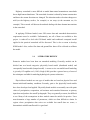
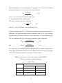
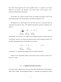
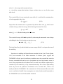
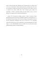
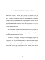
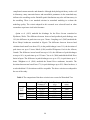
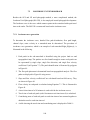
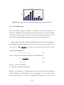
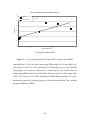
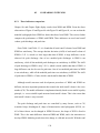
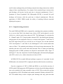
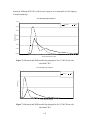
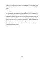
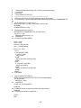
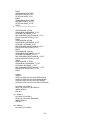
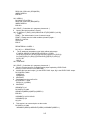
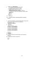
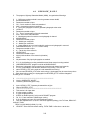
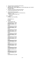
Assuming that the water table recharge and the soil transmissivity are spatially constant,
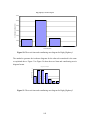
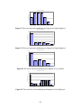
then ln r and ln T0 are eliminated from Equation (2.25) and Si is expressed as:
⎛
ai
S i = S + m ⋅ ⎜⎜ λ − ln
tan β i
⎝
⎞
⎟⎟
⎠
(2.26)
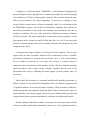
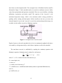
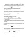
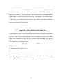
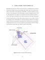
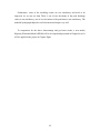
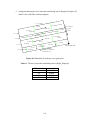
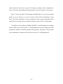
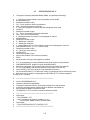
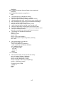
where λ is the areal average of the topographic index:
A
⎛ a
1
λ = ⋅ ∫ ln⎜⎜ i
A 0 ⎝ tan β i
⎞
⎟⎟ ⋅ Ai ⋅ dA
⎠
(2.27)
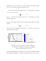
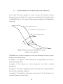
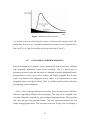
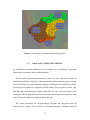
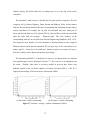
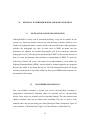
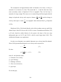
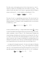
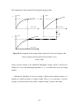
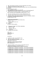
At each topographic index class λi , unsaturated and saturated zone fluxes are modeled.
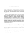
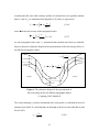
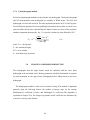
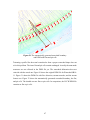
Figure 6 shows the schematic diagram of the representation of the local storage deficit, Si,
for different topographic indices.
⎛ a
⎞
λi = ln⎜⎜ i ⎟⎟
⎝ tan βi ⎠
Un-saturated aquifer
Un-saturated aquifer
Saturated aquifer
Saturated aquifer
⎛
a ⎞
Si = S + m ⋅ ⎜⎜ λ − ln i ⎟⎟
tan βi ⎠
⎝
S
Aquifuge
Aquifuge
Un-saturated aquifer
Saturated aquifer
Figure 6. The schematic diagram of the representation of
the local storage deficit for different topographic indices
(Campling, 2002, Modified)
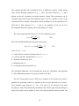
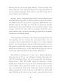
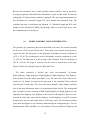
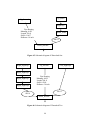
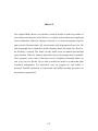
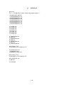
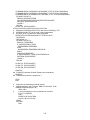
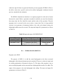
The vertical drainage qv from the unsaturated store at any point i is controlled by the local
saturated zone deficit Di, which depends on the depth of the local water table (Beven and
Wood, 1983):
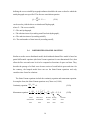
qv =
S uz
Di ⋅ t d
(2.28)
21