Download here - ESO

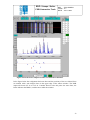
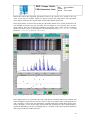
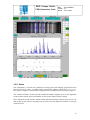
ESO Sampo Project
Reflex Subproject
FORS Interactive Tools
Document ref:
ESO-ERDA-
Version:
0.1
Authors:
Otto Solin
Acceptor:
Richard Hook
Released:
22 Nov 2007
ESO / Sampo / Reflex
FORS Interactive Tools
REF
: ESO-SAMPOISSUE : 0.1
DATE : 22.11.2007
TABLE OF CONTENTS
1.
INTRODUCTION .......................................................................................................... 3
1.1 Reference documents .....................................................................................................................3
2.
2.1
2.2
2.3
2.4
2.5
3.
3.1
3.2
3.3
3.4
3.5
4.
THE FORS WAVELENGTH CALIBRATION TOOL.............................................. 4
Inputs of the tool ............................................................................................................................4
Outputs of the tool..........................................................................................................................4
Python script ..................................................................................................................................4
Stand-alone usage ..........................................................................................................................5
Graphical interface.........................................................................................................................5
2.5.1 Buttons of the tool................................................................................................................6
2.5.2 Line identification window (all slits)...................................................................................7
2.5.2.1 Usage ...........................................................................................................................8
2.5.2.2 Mouse options .............................................................................................................8
2.5.2.3 Toolbar ........................................................................................................................9
2.5.3 Spectra of one slit, spectrum profile and results of fitting .................................................10
2.5.3.1 Single slit spectrum ...................................................................................................10
2.5.3.2 Spectrum profile ........................................................................................................12
2.5.3.3 Results of fitting ........................................................................................................13
2.5.4 Refitting one slit ................................................................................................................14
2.5.5 Deleting of line(s) ..............................................................................................................16
2.5.6 Recovering deleted line(s) .................................................................................................18
2.5.7 Changing the polynomial order of the fitting ....................................................................19
2.5.8 Notes ..................................................................................................................................20
FORS SKYLINE ALIGNMENT TOOL .................................................................... 21
Inputs of the tool ..........................................................................................................................21
Outputs of the tool........................................................................................................................21
Python script ................................................................................................................................22
Stand-alone usage ........................................................................................................................22
Graphical interface.......................................................................................................................23
3.5.1 Buttons of the tool..............................................................................................................23
3.5.2 Line identification window (all slits).................................................................................24
3.5.2.1 Usage .........................................................................................................................25
3.5.2.2 Mouse options ...........................................................................................................25
3.5.2.3 Toolbar ......................................................................................................................26
3.5.3 Spectra of one slit, spectrum profile and results of alignment...........................................27
3.5.3.1 Single slit spectrum ...................................................................................................28
3.5.3.2 Spectrum profile ........................................................................................................29
3.5.3.3 Results of alignment ..................................................................................................30
3.5.4 Realigning one slit .............................................................................................................31
3.5.5 Deleting of line(s) ..............................................................................................................32
3.5.6 Recovering deleted line(s) .................................................................................................35
3.5.7 Changing the polynomial order of the sky lines alignment ...............................................35
3.5.8 Notes ..................................................................................................................................37
SOME CONSIDERATIONS ....................................................................................... 38
4.1 Pros ..............................................................................................................................................38
II
ESO / Sampo / Reflex
FORS Interactive Tools
REF
: ESO-SAMPOISSUE : 0.1
DATE : 22.11.2007
4.2 Problems ......................................................................................................................................38
3
ESO / Sampo / Reflex
FORS Interactive Tools
1.
REF
: ESO-SAMPOISSUE : 0.1
DATE : 22.11.2007
INTRODUCTION
As an example of a Python script in a pipeline workflow, two interactive tools using Python
and matplotlib have been developed for the FORS instrument. FORS is the visual and near
UV FOcal Reducer and low dispersion Spectrograph for the VLT. It is the other one of the
two instruments chosen as examples for the Reflex beta-version.
The FORS wavelength calibration tool (Chapter 2) allows the user to view the results of the
wavelength calibration of slit spectra. This tool loops around the recipe
fors_wave_calib(_lss) and so applies to workflows involving master calibration
product creation (see Figure 8.3.1 in [2]). The Reflex distribution kit contains one example
workflow:
reflex/reflex-current/examples/FORSwavelenCalib_specTool.xml.
The FORS skyline alignment tool (Chapter 3) allows the user to view the results of the
alignment of the above mentioned wavelength solution (based on arc lamp spectra) to a set of
sky lines observed on a scientific exposure. This tool loops around the recipes
fors_align_sky(_lss) and fors_resample and so applies to workflows involving
science product creation (see Figure 8.3.2 in [2]). The Reflex distribution kit contains one
example workflow: reflex/reflex-current/examples/FORSalignSky.xml.
These two tools have a very similar interface. Some parts in chapters 2 and 3 are totally or
almost identical.
Parts of this document are identical to [3].
1.1
Reference documents
[1]
FORS Pipeline Web Page
http://www.eso.org/projects/dfs/dfs-shared/web/fors/fors-pipe-recipes.html
[2]
FORS Pipeline User Manual downloadable from [1]
ftp://ftp.eso.org/pub/dfs/pipelines/fors/fors-manual-1.2.pdf
[3]
Sampo Project Web Page
http://www.eso.org/sampo/reflex/instructions/interactive_tools.php
3
ESO / Sampo / Reflex
FORS Interactive Tools
2.
REF
: ESO-SAMPOISSUE : 0.1
DATE : 22.11.2007
THE FORS WAVELENGTH CALIBRATION TOOL
The FORS wavelength calibration tool can be run either within Reflex or stand-alone. The
purpose of the tool is to view and modify the results of the line fitting done by the recipe
fors_wave_calib or fors_wave_calib_lss. In the classification tags below the
MXU acronym can be read also as MOS or LSS.
2.1
Inputs of the tool
Inputs of fors_wave_calib(lss)
•
•
•
•
•
•
•
SPATIAL_MAP_MXU: map of spatial positions on the CCD i.e. the distance from the
top edge of the spectrum for each pixel
CURV_COEFF_MXU: the coefficients of the spectral curvature fitting polynomials
(not in case of LSS(like) data)
RECTIFIED_LAMP_MXU: spatially rectified arc lamp image (not in case of
LSS(like) data)
LAMP_UNBIAS_MXU: unbiased arc lamp exposure (only in case of LSS(like) data)
SLIT_LOCATION_MXU: slit positions
MASTER_LINECAT: the reference wavelengths for the arc lamp used
GRISM_TABLE: a subset of recipe configuration parameters
Outputs of fors_wave_calib(_lss)
•
•
•
•
•
•
2.2
•
•
2.3
REDUCED_LAMP_MXU: rectified and wavelength calibrated arc lamp image
DISP_COEFF_MXU: the wavelength calibration polynomial coefficients
DISP_RESIDUALS_MXU: residuals of each wavelength calibration fit
WAVELENGTH_MAP_MXU: map of wavelengths at the center of each pixel on the
CCD
SPECTRAL_RESOLUTION_MXU: mean spectral resolution for each reference arc
lamp line
SLIT_LOCATION_MXU: slit positions (only in case of LSS(like) data)
Outputs of the tool
the outputs of fors_wave_calib(_lss) (see above) refilled (except for
SPECTRAL_RESOLUTION_MXU) according to changed slit(s)
a fits table indicating slit(s) from where the user removed line(s)
Python script
The Python FORS wavelength calibration tool consists of two files:
forswavecalibtool.py is a launcher script and reflex.py contains Reflex usage
specific
module.
Both
scripts
are
located
under
reflex/reflexcurrent/scripts/python in the distribution kit.
4
ESO / Sampo / Reflex
FORS Interactive Tools
2.4
REF
: ESO-SAMPOISSUE : 0.1
DATE : 22.11.2007
Stand-alone usage
Run tool with default inputs in directory ./data.
python forswavecalibtool.py –d
You can also give the individual locations of the input files as parameter. The command
below corresponds to the command above except for the parameter specStep.
python forswavecalibtool.py specStep=2
Other parameters
•
•
-help shows the input parameters
-q makes a Reflex query
Clean-up
Note that when using the tool stand-alone, the user has to take care of cleaning the results
directory every now and then, e.g.:
rm -rf /tmp/reflex_tmp_forsSpecTool-*
2.5
Graphical interface
The example screenshot below is right after start-up. The example in the picture below is for
the seventh row in the eleventh slit. In this example there are 21 slits containing 709 rows in
total.
5
ESO / Sampo / Reflex
FORS Interactive Tools
REF
: ESO-SAMPOISSUE : 0.1
DATE : 22.11.2007
Figure 1: Wavelength calibration tool at start-up.
2.5.1 Buttons of the tool
Exit the tool.
Return all windows to original mode in current slit and image row.
For toggling between linear and logarithmic scale in
rectified/reduced lamp spectrum profile window (middle right side).
Move/zoom the three right side windows in horizontal
direction. See below note for matplotlib pan/zoom mode.
Move to preceding and subsequent image row.
Toggle between displaying slit number or slit ID in the slit buttons displayed
below in two columns, current mode is painted gray.
Clicking a slit button will display the center image row of the chosen slit.
Current slit is green.
Return to initial values.
Refit the current slit with new polynomial fitting order (IdsOrder) and/or
deleted/recovered lines. Refitting means rerunning the recipe fors_wave_calib
with EsoRex.
6
ESO / Sampo / Reflex
FORS Interactive Tools
REF
: ESO-SAMPOISSUE : 0.1
DATE : 22.11.2007
Decrease/increase the wavelength calibration polynomial order,
valid range is 2-5.
Toggle between different images (residuals of fit, non-linear part of fit,
pixel versus wavelength) in the fit results window (lower right side),
the next available mode is printed on the button.
Toggle x-axis between pixels and wavelengths in the three right side windows.
The two upper windows (single slit and spectrum profile window) are toggled between
RECTIFIED_LAMP_MXU (x-axis in pixels) and REDUCED_LAMP_MXU (x-axis in λ),
the next available mode is printed on the button.
Change the cuts of the images in the all slits and single slit windows.
2.5.2 Line identification window (all slits)
Window image shows the slit locations and spectra with identified lines which are plotted
over the spectra. The lines illuminate the grade of quality with current line catalogue and
inverse dispersion solution polynomial fitting order. The goal is to find anomalies in
identified line locations.
This window is an overview of RECTIFIED_LAMP_MXU of all slits with x-axis always in
pixels. The upper right side window shows one slit.
7
ESO / Sampo / Reflex
FORS Interactive Tools
REF
: ESO-SAMPOISSUE : 0.1
DATE : 22.11.2007
Figure 2: Line identification window.
2.5.2.1
Usage
Slit number and slit identification number are shown on top of the image window. Left side
shows the slit upon which the cursor is currently and right side is the selected (activated by
clicking) slit.
2.5.2.2
Mouse options
When moving mouse over image the slit under mouse pointer will be highlighted and
surrounded by a yellow box.
The slit can be selected by clicking the left mouse button. Selected slit will be highlighted
yellow.
Current image row is shown with a red bar over the current slit.
8
ESO / Sampo / Reflex
FORS Interactive Tools
2.5.2.3
REF
: ESO-SAMPOISSUE : 0.1
DATE : 22.11.2007
Toolbar
The matplotlib default toolbar has options which are useful for the image zooming and
panning.
The home button will return the image as it was in launch. A known problem is that in this tool
this does not always work properly (e.g. when spectrum profile window is in logarithmic scale).
Left and right arrows will work as a 'undo' and 'redo' when zooming or panning image.
Pan with left mouse, zoom with right. NOTE: matplotlib pan/zoom mode must be applied to
the single slit window, and when mouse button is released the changes done will reflect to the
two windows below it keeping the x-axis scale identical in all the three right side windows.
Note that the script blocks moving/zooming the single slit window in vertical direction.
Zoom area to rectangle.
9
ESO / Sampo / Reflex
FORS Interactive Tools
REF
: ESO-SAMPOISSUE : 0.1
DATE : 22.11.2007
2.5.3 Spectra of one slit, spectrum profile and results of fitting
The right-hand side of the tool window has three windows.
When x-axis is in pixels, active area of slit is painted light gray in the two lower windows.
Figure 3: Spectra of one slit, spectrum profile and results of fitting.
2.5.3.1
Single slit spectrum
The upper right side window plots the current single slit (highlighted in the left-side window).
Current image row is shown with a red bar. Image row can be chosen by clicking on single
slit window, but NOT in matplotlib pan/zoom mode.
The dispersion solutions for the identified lines calculated with the wavelength calibration
polynomial coefficients are shown with blue lines.
10
ESO / Sampo / Reflex
FORS Interactive Tools
REF
: ESO-SAMPOISSUE : 0.1
DATE : 22.11.2007
For zoom/move buttons see above where all the buttons are explained.
When x-axis is in pixels, the single slit and spectrum profile windows contain the
RECTIFIED_LAMP_MXU (produced by fors_extract_slits) versus x CCD position
of the current image row.
Figure 4: Single slit spectrum, x-axis in pixels.
When x-axis is wavelengths, the single slit and spectrum profile windows contain the rectified
and wavelength calibrated arc lamp image (REDUCED_LAMP_MXU) produced by
fors_wave_calib) versus wavelength.
Figure 5: Single slit spectrum, x-axis in wavelengths.
11
ESO / Sampo / Reflex
FORS Interactive Tools
2.5.3.2
REF
: ESO-SAMPOISSUE : 0.1
DATE : 22.11.2007
Spectrum profile
Figure 6: RECTIFIED_LAMP_MXU spectrum profile of image row 363, x-axis in pixels.
The middle right side window shows the spectrum profile of one image row. The current
image row is printed above the window: the current slit contains 12 rows and all the slits
together contain 709 rows.
The peak positions of the spectrum are marked with red triangles. The identified line
wavelength is printed above the peak.
RECTIFIED_LAMP_MXU has in this example 2048 columns and 709 rows. The x-coordinate
for the peak position in Figure 6 is taken from the nth column where n is the pixel value
calculated from the fitting polynomial:
d
x = ∑ cn (λ − λ0 ) n (1)
n =0
where
•
•
•
•
x is the x CCD pixel position
c 0 ….c 5 are the model coefficients taken from DISP_COEFF_MXU for each
image row
λ 0 is the central wavelength of the grism used
d is the degree of the fitting polynomial that can be changed with the buttons
around IdsOrder for refitting one slit
To x is added the residual of the fit, and half a pixel is subtracted to compensate for half-pixel
mismatch between different conventions between recipes and matplotlib of plotting data. The
y position for the peak position in Figure 6 is the xth column for the current image row.
REDUCED_LAMP_MXU has in this example 1697 columns 709 rows. The x coordinate for the
peak position in Figure 7 is directly from the line catalog. The column index in
REDUCED_LAMP_MXU for the y coordinate is:
12
ESO / Sampo / Reflex
REF
: ESO-SAMPOISSUE : 0.1
DATE : 22.11.2007
FORS Interactive Tools
index = int(
where
•
•
λ − CRVAL1
CD1 _ 1
+ 0,5)
(2)
λ is the line catalog wavelength
index is the number of the column in REDUCED_LAMP_MXU
Figure 7: REDUCED_LAMP_MXU spectrum profile of image row 363, x-axis in
wavelengths.
2.5.3.3
Results of fitting
The lower right side window plots at start-up the residuals of the fit versus x CCD position for
the current image row.
Lines outside active area or not found by the fitting are indicated with a black triangle down
in the upper edge of the window.
Figure 8: Residuals of the fitting, x-axis in pixels.
13
ESO / Sampo / Reflex
FORS Interactive Tools
REF
: ESO-SAMPOISSUE : 0.1
DATE : 22.11.2007
Figure 8 shows the fit residuals of the identified peaks. The residuals are read from row 363
of the DISP_RESIDUALS_MXU image, where are collected all the residuals (in pixels) of the
derived wavelength calibration with respect to the measured pixel positions of the reference
arc lamp lines with x pixels corresponding to the original CCD pixels, and y pixels
corresponding to the REDUCED_LAMP_MXU pixels (i.e. to the rectified spatial coordinate).
Typical observed residuals should be around 0.2 pixels. Note that in this image all residuals
are shown, including those from lines that were excluded from the polynomial fit, i.e.
residuals larger than the threshold specified with the configuration parameter –wreject, but
this tool shows these as lines not found, i.e. with a black triangle down in the upper edge of
window.
In addition to residuals the non-linear part of the fitting and pixel position can be plotted
(second button from the left below window).
The x-axis can be toggled between pixels and wavelength (first button from the left below
window). When x-axis is in wavelengths, the value of the residuals (y axis) in Ångströms is
computed by multiplying the value (in pixels) in the DISP_RESIDUALS_MXU image with
the keyword CD1_1.
Figure 9: Non-linear part of the fitting, x-axis in wavelengths.
Figure 9 shows the deviation of the identified peaks from the linear term of the 363th fitting
polynomial. The solid line is the polynomial model (Equation (1)) with the linear term
subtracted.
2.5.4 Refitting one slit
Refitting means rerunning the recipe fors_wave_calib, that is used for deriving a
wavelength calibration (made following the spectral curvature), with new polynomial fitting
order and/or new line catalog where lines have been deleted/recovered.
Of all the parameters of fors_wave_calib, the tool can modify only –-wdegree, the
polynomial order of the fitting.
Normally this recipe would calibrate all the slit spectra at once, but this tool makes it work for
a single slit spectrum at a time. The input data is modified in such a way that it looks like on
the CCD just one spectrum is present. The inputs of the tool are listed in Chapter 2.1 and the
outputs in Chapter 2.2. The tool creates the set of inputs for fors_wave_calib by slicing
lanes from the inputs for all slit spectra:
14
ESO / Sampo / Reflex
FORS Interactive Tools
•
•
•
•
REF
: ESO-SAMPOISSUE : 0.1
DATE : 22.11.2007
From SLIT_LOCATION_MXU the row where the 1st column is the slit identification
number slit_id of the slit to be refitted. So this input will contain only one row.
From CURV_COEFF_MXU a lane of two rows where the 1st column is the slit_id
of the slit to be refitted.
From RECTIFIED_LAMP_MXU a lane with starting row and length (number of
rows) indicated by position and length in SLIT_LOCATION_MXU in the last
two columns of the row starting with slit_id of the slit to be refitted.
SPATIAL_MAP_MXU, MASTER_LINECAT and GRISM_TABLE are used as-is.
The tool recreates the set of outputs of fors_wave_calib by refilling in the outputs the area
corresponding to the refitted slit:
•
•
•
In REDUCED_LAMP_MXU, DISP_COEFF_MXU and DISP_RESIDUALS_MXU a
lane with starting row and length indicated by position and length in
SLIT_LOCATION_MXU in the last two columns of the row starting with slit_id
of the refitted slit.
WAVELENGTH_MAP_MXU is refilled with all non-zero values of the file produced for
one slit (the dimensions of this fits file are the same when produced for one slit or all
slits)
SPECTRAL_RESOLUTION_MXU is used as-is.
It is crucial to upgrade the global wavelength map of the CCD (WAVELENGTH_MAP_MXU)
and the table containing the wavelength calibration polynomial coefficients of all the spectra
(DISP_COEFF_MXU): these two files will be used in the reduction of the scientific frames.
This merging is performed also on the other products even if they are just meant for check
purposes; they are "nice to have".
15
ESO / Sampo / Reflex
FORS Interactive Tools
REF
: ESO-SAMPOISSUE : 0.1
DATE : 22.11.2007
2.5.5 Deleting of line(s)
Click with left mouse button blue ball(s) in the lower window. The ball will turn red and
activate the fit-button. You can cancel your intended deletion with right mouse button. The
refit is done by pressing the fit-button. After refitting, a red triangle down in the upper edge of
the fit results window will indicate the line(s) deleted by the user.
In the figure below two lines with clearly larger residuals are marked for deletion and the fitbutton is active. In the slit columns are shown the slit IDs.
Figure 10: In the lower subplot two lines are marked for deletion.
16
ESO / Sampo / Reflex
FORS Interactive Tools
REF
: ESO-SAMPOISSUE : 0.1
DATE : 22.11.2007
In the figure below the refitting has been done and the positions of the two deleted lines are
marked with a red triangle down in the upper edge of the fit results window. The RMS
improved from 0.071 to 0.027. Consider however also this point: the more lines, the better
indicator the RMS is, and the more stable the solution.
Figure 11: The previous figure after refitting.
The tool produces a fits table that keeps track of the lines deleted by the user. The first two
columns are a copy of the original line catalog. When a line is removed from a slit, a new
column with the removed line(s) set to zero is added.
17
ESO / Sampo / Reflex
FORS Interactive Tools
REF
: ESO-SAMPOISSUE : 0.1
DATE : 22.11.2007
Figure 12: The zeros in the rightmost column indicate deleted lines.
2.5.6 Recovering deleted line(s)
Deleted lines can be recovered by clicking with left mouse button the red triangle down
turning it blue. You can cancel your intended recovering with right mouse button.
In the figure below the other one of the two lines deleted in the previous step is marked for
recovery and the fit-button is active.
Figure 13: One of two deleted lines is marked for recovery.
18
ESO / Sampo / Reflex
FORS Interactive Tools
REF
: ESO-SAMPOISSUE : 0.1
DATE : 22.11.2007
2.5.7 Changing the polynomial order of the fitting
Click either arrow beside the IdsOrder box to decrease/increase the polynomial order. This
will activate (turn green) the fit-button. The refit is done by pressing the fit-button after which
the polynomial order of the current slit is stored to the new value. If you move to another
image row before pressing the fit-button, the polynomial order will be restored to the original
value and the fit-button deactivated.
In the figure below we first of all see that the slit button number 20 is yellow because this slit
was changed in the previous step. Secondly the reset-button is active (green) since we have
made changes. Now we decrease the polynomial fitting order of the current (slit button
number 6 is green) slit and refit it. The tool runs the recipe fors_wave_calib with
parameter --wdegree set to IdsOrder.
Figure 14: Polynomial order changed for slit number 6, but not yet refitted.
In the figure below we see that the previous step was not a good idea since RMS worsened
from 0.06 to 0.082.
19
ESO / Sampo / Reflex
FORS Interactive Tools
REF
: ESO-SAMPOISSUE : 0.1
DATE : 22.11.2007
In the fits table disp_coeff_mxu_new.fits produced by the tool (that reruns
fors_wave_calib), you will see that column c4 of the rows 500-533 has changed to
zero. These rows correspond slit number 6 for which we changed the fitting order from 4 to 3.
Increasing the order to 5 would create column c5.
Figure 15: Slit number 6 refitted with new polynomial order.
2.5.8 Notes
The refit is in both cases (deleting/recovering lines and changing fit order) done for one slit at
a time. A refitted slit is indicated by painting yellow the IdsOrder box and the slit button.
After the first refit the reset-button is activated (turned green).
The combined number of blue/red balls and black/red/blue triangles down in the fit results
window equals always the number of lines in the original line catalog.
In the fit results window red/blue balls and black triangles down are per image row, red/blue
triangles down are per slit. Note the difference with the skyline alignment tool.
20
ESO / Sampo / Reflex
FORS Interactive Tools
3.
REF
: ESO-SAMPOISSUE : 0.1
DATE : 22.11.2007
FORS SKYLINE ALIGNMENT TOOL
The FORS skyline alignment tool can be run either within Reflex or stand-alone. The purpose
of the tool is to view and modify the results of the skyline alignment done by the recipes
fors_align_sky(_lss) and fors_resample. In the classification tags below the
MXU acronym can be read also as MOS or LSS.
3.1
Inputs of the tool
Inputs of fors_align_sky(_lss)
•
•
•
•
•
•
•
•
SPATIAL_MAP_MXU: map of spatial positions on the CCD i.e. the distance from the
top edge of the spectrum for each pixel (not in case of LSS(like) data)
CURV_COEFF_MXU: spectral curvature coefficients (not in case of LSS(like) data)
DISP_COEFF_MXU: wavelength solution coefficients
RECTIFIED_ALL_SCI_MXU: spatially rectified slit spectra (not in case of
LSS(like) data)
SCIENCE_UNFLAT_MXU: flat field corrected science frame (only in case of
LSS(like) data)
SLIT_LOCATION_MXU: slit positions
MASTER_SKYLINECAT: the reference wavelengths of the sky lines used for
adjusting the input wavelength solution to the observed scientific spectra
GRISM_TABLE: a subset of recipe configuration parameters
Outputs of fors_align_sky(_lss)
•
•
•
SKY_SHIFTS_SLIT_SCI_MXU, or SKY_SHIFTS_LONG_SCI_MXU in case of
LSS(like) data: the observed sky lines offsets for adjusting the input wavelength
solutions
WAVELENGTH_MAP_SCI_MXU: map of wavelengths at the center of each pixel on
the CCD, upgraded from WAVELENGTH_MAP_MXU
DISP_COEFF_SCI_MXU: the DISP_COEFF_MXU after alignment of the solutions
to the position of the sky lines
Outputs of fors_resample
•
3.2
•
•
MAPPED_ALL_SCI_MXU: rectified and wavelength calibrated slit spectra
Outputs of the tool
the outputs of fors_align_sky(_lss) and fors_resample (see above)
refilled according to changed slit(s)
a fits table indicating slit(s) from where the user removed line(s)
21
ESO / Sampo / Reflex
FORS Interactive Tools
3.3
REF
: ESO-SAMPOISSUE : 0.1
DATE : 22.11.2007
Python script
The Python FORS wavelength calibration tool consists of two files: FORSalignSky.py is
a launcher script and reflex.py contains Reflex usage specific module. Both scripts are
located under reflex/reflex-current/scripts/python in the distribution kit.
3.4
Stand-alone usage
Run tool with default inputs in directory ./data.
python FORSalignSky.py –d
You can also give the individual locations of the input files as parameter. The command
below corresponds to the command above except for the parameter specStep.
python FORSalignSky.py specStep=2
Other parameters
•
•
-help shows the input parameters
-q makes a Reflex query
Clean-up
Note that when using the tool stand-alone, the user has to take care of cleaning the results
directory every now and then, e.g.:
rm -rf /tmp/reflex_tmp_forsSpecTool-*
22
ESO / Sampo / Reflex
FORS Interactive Tools
3.5
REF
: ESO-SAMPOISSUE : 0.1
DATE : 22.11.2007
Graphical interface
The example screenshot below is right after start-up. The example in the picture below is for
the seventh row in the eleventh slit. In this example there are 21 slits containing 709 rows in
total.
Figure 16: Skyline alignment tool at start-up
3.5.1 Buttons of the tool
Exit the tool.
Return all windows to original mode in current slit and image row.
For toggling between linear and logarithmic scale in
rectified/reduced lamp spectrum profile window (middle right side).
Move/zoom the three right side windows in horizontal
direction. See below note for matplotlib pan/zoom mode.
Move to preceding and subsequent image row.
23
ESO / Sampo / Reflex
FORS Interactive Tools
REF
: ESO-SAMPOISSUE : 0.1
DATE : 22.11.2007
Toggle between displaying slit number or slit ID in the slit buttons displayed
below in two columns, current mode is painted gray.
Clicking a slit button will display the center image row of the chosen slit.
Current slit is green.
Return to initial values.
Realign the current slit with new alignment polynomial order (AlignOrder) and/or
deleted/recovered lines. Realigning means rerunning the recipes fors_ align_sky
and fors resample with EsoRex.
Decrease/increase the polynomial order for sky lines alignment,
valid range is 0-2.
Toggle x-axis between pixels and wavelengths in the three right side windows.
The two upper windows (single slit and spectrum profile window) are toggled between
RECTIFIED_ALL_SCI_MXU (x-axis in pixels) and MAPPED_ALL_SCI_MXU (xaxis in λ), the next available mode is printed on the button.
Change the cuts of the images in the all slits and single slit windows.
3.5.2 Line identification window (all slits)
Window image shows the slit locations and spectra with skylines which are plotted over the
spectra. The lines illuminate the grade of quality with current skyline catalogue and inverse
dispersion solution polynomial fitting order. The goal is to find anomalies in identified
skyline locations.
This window is an overview of RECTIFIED_ALL_SCI_MXU of all slits with x-axis always
in pixels. The upper right side window shows one slit.
24
ESO / Sampo / Reflex
FORS Interactive Tools
REF
: ESO-SAMPOISSUE : 0.1
DATE : 22.11.2007
Figure 17: Line identification window.
3.5.2.1
Usage
Slit number and slit identification number are shown on top of the image window. Left side
shows the slit upon which the cursor is currently and right side is the selected (activated by
clicking) slit.
3.5.2.2
Mouse options
When moving mouse over image the slit under mouse pointer will be highlighted and
surrounded by a yellow box.
The slit can be selected by clicking the left mouse button. Selected slit will be highlighted
yellow.
Current image row is shown with a red bar over the current slit.
25
ESO / Sampo / Reflex
FORS Interactive Tools
3.5.2.3
REF
: ESO-SAMPOISSUE : 0.1
DATE : 22.11.2007
Toolbar
The matplotlib default toolbar has options which are useful for the image zooming and
panning.
The home button will return the image as it was in launch. A known problem is that in this tool
this does not always work properly (e.g. when spectrum profile window is in logarithmic scale).
Left and right arrows will work as a 'undo' and 'redo' when zooming or panning image.
Pan with left mouse, zoom with right. NOTE: matplotlib pan/zoom mode must be applied to
the single slit window, and when mouse button is released the changes done will reflect to the
two windows below it keeping the x-axis scale identical in all the three right side windows.
Note that the script blocks moving/zooming the single slit window in vertical direction.
Zoom area to rectangle.
26
ESO / Sampo / Reflex
FORS Interactive Tools
REF
: ESO-SAMPOISSUE : 0.1
DATE : 22.11.2007
3.5.3 Spectra of one slit, spectrum profile and results of alignment
The right-hand side of the tool window has three windows.
When x-axis is in pixels, active area of slit is painted light gray in the two lower windows.
Figure 18: Spectra of one slit, spectrum profile and sky lines offsets.
27
ESO / Sampo / Reflex
FORS Interactive Tools
3.5.3.1
REF
: ESO-SAMPOISSUE : 0.1
DATE : 22.11.2007
Single slit spectrum
The upper right side window plots the current single slit (highlighted in the left-side window).
Current image row is shown with a red bar. Image row can be chosen by clicking on single
slit window, but NOT in matplotlib pan/zoom mode.
The dispersion solutions for the identified lines calculated with the wavelength calibration
polynomial coefficients are shown with blue lines.
For zoom/move buttons see above where all the buttons are explained.
When x-axis is in pixels, the single slit and spectrum profile windows contain the
RECTIFIED_ALL_SCI_MXU (produced by fors_extract_slits) versus x CCD
position of the current image row.
Figure 19: Single slit spectrum, x-axis in pixels.
When x-axis is wavelengths, the single slit and spectrum profile windows contain the
MAPPED_ALL_SCI_MXU (produced by fors_resample) versus wavelength.
Figure 20: Single slit spectrum, x-axis in wavelengths.
28
ESO / Sampo / Reflex
FORS Interactive Tools
3.5.3.2
REF
: ESO-SAMPOISSUE : 0.1
DATE : 22.11.2007
Spectrum profile
Figure 21: RECTIFIED_ALL_SCI_MXU spectrum profile of image row 363, x-axis in
pixels.
The middle right side window shows the spectrum profile of one image row. The current
image row is printed above the window: the current slit contains 12 rows and all the slits
together contain 709 rows.
The peak positions of the spectrum are marked with red triangles. The identified line
wavelength is printed above the peak.
RECTIFIED_ALL_SCI_MXU has in this example 2048 columns and 709 rows. The xcoordinate for the peak position in Figure 21 is taken from the xth column where x is the pixel
value calculated from the fitting polynomial:
d
x = ∑ cn (λ − λ0 ) n (3)
n =0
where
•
•
•
•
x is the x CCD pixel position
c 0 ….c 5 are the model coefficients taken from DISP_COEFF_SCI_MXU for
each image row
λ 0 is the central wavelength of the grism used
d is the degree of the fitting polynomial that was used for the wavelength
calibration
To x is added the sky lines offset of the current slit, and half a pixel is subtracted to
compensate for half-pixel mismatch between different conventions between recipes and
matplotlib of plotting data. The y position for the peak position in Figure 21 is the xth column
for the current image row.
MAPPED_ALL_SCI_MXU has in this example 1697 columns 709 rows. The x coordinate for
the peak position in Figure 22 is directly from the line catalog. The column index in
MAPPED_ALL_SCI_MXU for the y coordinate is:
29
ESO / Sampo / Reflex
FORS Interactive Tools
index = int(
where
•
•
λ − CRVAL1
CD1 _ 1
+ 0,5)
REF
: ESO-SAMPOISSUE : 0.1
DATE : 22.11.2007
(4)
λ is the line catalog wavelength
index is the number of the column in MAPPED_ALL_SCI_MXU
Figure 22: MAPPED_ALL_SCI_MXU spectrum profile of image row 363, x-axis in
wavelengths.
3.5.3.3
Results of alignment
The lower right side window plots the observed sky lines offsets of the alignment for the
current slit (NOTE that unlike residuals in the wavelength calibration tool, the offsets are here
per slit and not per image row).
Lines outside active area or not found by the alignment are indicated with a black triangle
down in the upper edge of window.
30
ESO / Sampo / Reflex
FORS Interactive Tools
REF
: ESO-SAMPOISSUE : 0.1
DATE : 22.11.2007
Figure 23: Sky lines offsets, x-axis in pixels.
Figure 23 shows the sky lines offsets of the identified peaks. They are read from column
offset11 of the SKY_SHIFTS_SLIT_SCI_MXU table containing the observed sky lines
offsets (in pixels) that were used for adjusting the input wavelength solution.
The x-axis can be toggled between pixels and wavelength (first button from the left below
window). When x-axis is in wavelengths, the value of the offsets (y axis) in Ångströms is
computed by multiplying the value (in pixels) in the SKY_SHIFTS_SLIT_SCI_MXU table
with the keyword CD1_1.
Figure 24: Sky lines offsets, x-axis in wavelengths.
3.5.4 Realigning one slit
Realigning means rerunning the recipes fors_align_sky, that adjusts the input
wavelength calibration to the observed positions of a set of sky lines, and fors_resample,
that resamples the original spectrum at a constant wavelength step thus creating the image
with rectified and wavelength calibrated slit spectra.
31
ESO / Sampo / Reflex
FORS Interactive Tools
REF
: ESO-SAMPOISSUE : 0.1
DATE : 22.11.2007
Of all the parameters of fors_align_sky, the tool can modify only --skyalign, the
polynomial order of the alignment.
Normally this recipe would calibrate all the slit spectra at once, but this tool makes it work for
a single slit spectrum at a time. The input data is modified in such a way that it looks like on
the CCD just one spectrum is present. The inputs of the tool are listed in Chapter 3.1 and the
outputs in Chapter 3.2. The tool creates the set of inputs for fors_align_sky and
fors_resample by slicing lanes from the inputs for all slit spectra:
•
•
•
•
From SLIT_LOCATION_MXU the row where the 1st column is the slit identification
number slit_id of the slit to be refitted. So this input will contain only one row.
From CURV_COEFF_MXU a lane of two rows where the 1st column is the slit_id
of the slit to be refitted.
From RECTIFIED_ALL_SCI_MXU a lane with starting row and length (number of
rows) indicated by position and length in SLIT_LOCATION_MXU in the last
two columns of the row starting with slit_id of the slit to be refitted.
SPATIAL_MAP_MXU, MASTER_SKYLINECAT and GRISM_TABLE are used as-is.
The tool recreates the set of outputs of fors_align_sky and fors_resample by
refilling in the outputs the area corresponding to the refitted slit:
•
•
•
In DISP_COEFF_SCI_MXU and MAPPED_ALL_SCI_MXU a lane with starting row
and length indicated by position and length in SLIT_LOCATION_MXU in the
last two columns of the row starting with slit_id of the realigned slit.
In SKY_SHIFTS_SLIT_SCI_MXU the column offset<slit_id> with the one
produced by the tool.
WAVELENGTH_MAP_SCI_MXU is refilled with all non-zero values of the file
produced for one slit (the dimensions of this fits file are the same when produced for
one slit or all slits)
The
observed
sky
lines
offsets
from
their
expected
positions
(SKY_SHIFTS_SLIT_SCI_MXU) are fitted by polynomials that are then added to the input
wavelength
calibration
polynomials
(DISP_COEFF_MXU)
thus
creating
DISP_COEFF_SCI_MXU.
3.5.5 Deleting of line(s)
Click with left mouse button blue ball(s) in the lower window. The ball will turn red and
activate the align button. You can cancel your intended deletion with right mouse button. The
realignment is done by pressing the align-button. After realignment, a red triangle down in the
upper edge of the offsets window will indicate the line(s) deleted by the user.
In the figure below two lines with the largest offsets are marked for deletion and the alignbutton is active.
32
ESO / Sampo / Reflex
FORS Interactive Tools
REF
: ESO-SAMPOISSUE : 0.1
DATE : 22.11.2007
Figure 25: In the lower subplot two lines are marked for deletion.
In the figure below the realignment has been done and the positions of the two deleted lines
are marked with a red triangle down in the upper edge of the offsets window. The RMS
improved from 0.427 Å to 0.233 Å. Consider however also this point: the more lines, the
better indicator the RMS is, and the more stable the solution.
33
ESO / Sampo / Reflex
FORS Interactive Tools
REF
: ESO-SAMPOISSUE : 0.1
DATE : 22.11.2007
Figure 26: The previous figure after realignment.
The tool produces a fits table that keeps track of the lines deleted by the user. The first
column is a copy of the original line catalog. When a line is removed from a slit, a new
column with the removed line(s) set to zero is added.
34
ESO / Sampo / Reflex
FORS Interactive Tools
REF
: ESO-SAMPOISSUE : 0.1
DATE : 22.11.2007
Figure 27: The zeros in the rightmost column indicate deleted lines.
3.5.6 Recovering deleted line(s)
Deleted lines can be recovered by clicking with left mouse button the red triangle down
turning it blue. You can cancel your intended recovering with right mouse button.
In the figure below the other one of the two lines deleted in the previous step is marked for
recovery and the align-button is active.
Figure 28: One of two deleted lines is marked for recovery.
3.5.7 Changing the polynomial order of the sky lines alignment
Click either arrow beside the AlignOrder box to decrease/increase the polynomial order.
This will activate (turn green) the align-button. The realignment is done by pressing the align35
ESO / Sampo / Reflex
FORS Interactive Tools
REF
: ESO-SAMPOISSUE : 0.1
DATE : 22.11.2007
button after which the alignment polynomial order of the current slit is stored to the new
value. If you move to another image row before pressing the align button, the polynomial
order will be restored to the original value and the align button deactivated.
In the figure below we first of all see that the slit button number 14 is yellow because this slit
was changed in the previous step. Secondly the reset button is active (green) since we have
made changes. Now we increase the alignment polynomial order of the current (slit button
number 8 is green) slit to 1 and realign it. The tool runs the recipe fors_align_sky with
parameter --skyalign set to AlignOrder.
Figure 29: Polynomial order changed for slit number 8, but not yet realigned.
In the figure below we see that the previous step did not certainly improve the solution and
moreover RMS worsened from 0.276 Å to 0.58 Å. This is no surprise since in the general case
with --skyalign = 0 the recipe just determines a median offset from all the observed sky lines,
while --skyalign = 1 tries to fit a slope (rarely useful, but sometimes sky lines offsets display a
significant dependency on the wavelength, due to a variation of the mean spectral dispersion
with respect to the day calibrations) [2].
36
ESO / Sampo / Reflex
FORS Interactive Tools
REF
: ESO-SAMPOISSUE : 0.1
DATE : 22.11.2007
Figure 30: Slit number 8 realigned with new polynomial order.
3.5.8 Notes
The realignment is in both cases (deleting/recovering lines and changing polynomial order)
done for one slit at a time. A realigned slit is indicated by painting yellow the AlignOrder
box and the slit button. After the first realignment the reset-button is activated (turned green).
The combined number of blue/red balls and black/red/blue triangles down in the alignment
results window equals always the number of lines in the original skyline catalog.
In the alignment results window red/blue balls and black/red/blue triangles down are per slit
(that is they are the same for all image rows in a slit). Note the difference with the wavelength
calibration tool.
37
ESO / Sampo / Reflex
FORS Interactive Tools
4.
SOME CONSIDERATIONS
4.1
Pros
REF
: ESO-SAMPOISSUE : 0.1
DATE : 22.11.2007
The interactive tools offer the possibility to check the quality of the products and to fine-tune
the data reduction process.
The following point was raised by Carlo Izzo. The tools also offer a good incentive to
standardization. For instance, at the moment the wavelength calibration tools included in
Reflex can be used with FORS data only. They cannot be used on the VIMOS pipeline
products, which follow a completely different convention. And yet the VIMOS pipeline
products are essentially the same as the FORS ones! The existence of a tool for examining the
quality of MOS products in a given format would encourage any MOS pipeline to create
products that are conventionally formatted as required by this tool.
4.2
Problems
Everything presented here so far is perfectly nice. The interface of the tools looks good and
they operate meaningfully.
But the slowness of these tools threatens to make them unusable. More specifically: The
slowness of e.g. everything related to refitting is not such a big problem since running e.g.
fors_wave_calib takes ~10sec. But what is most worrying is the slowness in change
between views. In our example exposure there are 709 image rows. Changing image row can
be done e.g. by pressing ‘previous' or 'next' buttons. Doing for example this is so slow, that
these tools can never be adequate for effective checking of pipeline results. The user should
be able to view results in different slits/rows instantaneously. As a reference you only need to
compare the 'Zoom' and 'Flip' buttons of the Skycat tool to the 'Move' and 'Zoom' buttons of
our tool.
The reason for this slowness goes back to the decision to implement these tools with
Python/matplotlib. Initially these tools were much lighter, but since then they have grown too
big to be done with Python. Now these tools can be seen more as a demonstration of what a
tool could be. As an example of a Python script in a Reflex workflow they of course work
perfectly.
It should be evaluated whether there is need to create with C/C++ tools of this kind that work
fast enough.
38