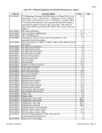
1
Using the PanCancer Immune Profiling Advanced Analysis Module NanoString Technologies®, Inc. www.nanostring.com OCTOBER 2015 USNS-PM0051-01 WHITE PAPER PanCancer Immune Profiling Advanced Analysis Module Using the PanCancer Immune Profiling Analysis Model for Analysis of nCounter® PanCancer Immune Profiling Data Introduction The PanCancer Immune Profiling Advanced Analysis Module was created to help scientists perform statistically-principled analyses of their nCounter PanCancer Immune Profiling Panel data. It brings together powerful academic open-source analysis tools via a simple interface that guides a user through the analysis to create an interactive HTML document that displays the analytical results. The collection of advanced analysis capabilities that define the PanCancer Immune Profiling Advanced Analysis Module includes eight modules enabling QC, Normalization, Immune Cell Scoring, CT Antigen Expression, Differential Expression (DE), Gene Set Analysis (GSA), Pathview Plots, and Select Gene Descriptions (SGD). These advanced analyses are performed using R, a powerful statistical software program. However, familiarity with R is not required, as users only need to interact with a simple wizard within nSolver™ 2.6. While users of the PanCancer Pathways Advanced Analysis Module will find many of the analysis options similar, the PanCancer Immune Profiling Advanced Analysis Module includes unique analytical methods for expression-based assessment of immune cell type activity. Genes defined as being cell type-specific are used to calculate cell type scores, and gene set analysis groups genes into functional immune-related categories. 3.) A window will open with options to create and run an R script. 4.) The script will run and store all data on a local computer (Results are not imported into nSolver, and the original data remains untouched.) 5.) The results are displayed in an HTML viewer (e.g., a web browser). The nSolver Analysis Software User Manual explains the basics of how to install and operate nSolver; this white paper will begin with the process of setting up an advanced analysis using the PanCancer Immune Profiling Panel Advanced Analysis Module. The analysis described below uses the example breast cancer data that is available when downloading nSolver and can be used as a training tool. These 74 samples are a subset of the 201 files provided with the Pan Cancer Immune Profiling panel, and sample names are the same to allow cross comparison. However, it should be noted that the control samples are different. Advanced analyses in nSolver 2.6 can only be applied to one of two levels of data: raw data or normalized data. An experiment must also be created within nSolver to run the advanced analysis. If raw data are used, then the PanCancer Immune Profiling Advanced Analysis Module can automatically choose optimal normalization genes and use them to perform normalization. Performing the advanced analysis using normalized data will preserve the normalization and/or background subtraction already performed in nSolver. Results of an advanced analysis are displayed in two formats: • Aresults directory containing the plots and tables created by the analysis • An interactive HTML analysis report. This white paper describes an example analysis detailing the choices available to the user and explaining the potential outcomes of these decisions in the results. It is presented in the style of a vignette that shows the complete analysis of an actual PanCancer Immune Profiling Panel dataset. Running the nCounter® PanCancer Immune Profiling Panel Advanced Analysis The workflow to operate the PanCancer Immune Profiling Advanced Analysis Module is very simple: 1.) Import RCC files to nSolver 2.6, perform QC, and create an experiment. 2.) Select the data to use and select Advanced Analysis. 2 FIGURE 1 Begin an advanced analysis. Select the desired samples from the Experiments view, and then select the Advanced Analysis icon. NanoString Technologies, Inc. WHITE PAPER FIGURE 2 FIGURE 4 Select the desired advanced analysis. Choose a name for the analysis, select an analysis module, and specify a path where the analysis files should be saved. Select sample annotations to be included in analysis. Select annotations, the data type (categorical or continuous) for each annotation, and the references for any categorical annotations. Once the advanced analysis wizard opens, choose a name for the analysis and select an analysis module. The PanCancer Immune Profiling Advanced Analysis Module will only work with files generated using the PanCancer Immune Profiling Panel and its accompanying Reporter Library File (RLF). Specific analysis modules are available for Human and Mouse and offer identical functionality with only a few differences in the underlying gene and cell type annotations. Data generated by merging a PanCancer Immune Profiling Panel RLF with an Add-in Library File (ALF) are also compatible with the analysis module. However, the additional genes specified in the ALF will be ignored. Click Next to continue to the sample annotations screen. Select Sample Annotations The annotations screen is the first of four screens in which analysis parameters are entered. Any annotations created in nSolver when setting up the experiment are available. To import additional annotations in the advanced analysis wizard, select Import. Once all the annotations have been imported, select one variable to serve as a unique identifier for every lane. In this case, Sample Name has been selected using the checkbox in the first column. (The *.RCC file name will always be a valid identifier. However, these file names tend to be lengthy.) Next, select the annotations (covariates) to be used in the analysis. Only the covariates selected here will be available in later steps of the analysis. In most experiments, it will be appropriate to include one or more biological annotations in the analysis. It can also be useful to include technical annotations, either to confirm that they are not influencing the results or to account for their effects in the analysis. For example, CodeSet lot and hybridization time may be technical annotations that deserve consideration. Three types of annotations – categorical, continuous, and true/ false – can be included in the advanced analysis. nSolver attempts to provide logical default annotation types. However, review these before continuing the analysis. It is also necessary to specify a categorical reference for each categorical connotation. These will be used for comparison. Categorical: These are annotations for which the samples exist in a number of distinct categories. In this example, Subtype and Tumor Grade are categorical. A categorical covariate may contains text or numbers but must always have a defined “categorical reference” or baseline. The choice of a reference shapes differential expression analysis, which will compare all variations of the categorical annotation to the chosen reference. FIGURE 3 Import an annotation set. Select an annotation file and the annotations to be imported. 3 WHITE PAPER PanCancer Immune Profiling Advanced Analysis Module Continuous: These annotations have values that can be interpreted meaningfully as numbers. Binding Density is a good example of a continuous variable: if two samples have binding densities of 1.0 and 1.2, this can be interpreted to mean the second sample has binding density 0.2 units greater than the first. However, some numeric variables, such as Disease Grade, describe more arbitrary measures. Classifying this annotation as “continuous” would be dubious because it would imply that the difference between Grade I and Grade II disease is the same as the difference between Grade II and Grade III, i.e., one “unit” of disease. Numeric variables like Disease Grade are thus better modeled as categorical annotations. True/False: These annotations must take only the values TRUE or FALSE. For the purposes of the PanCancer Immune Profiling Advanced Analysis Module, such annotations are equivalent to categorical annotations with FALSE as the reference level. This example dataset contains results from 74 breast cancer and healthy breast tissue samples assayed with the PanCancer Immune Profiling Panel. For each cancer sample, the subtype is known and was annotated in nSolver as Normal, A, B, C, or D. The biological annotation Subtype was selected for the analysis. Other Annotations Chosen For This Analysis: • Binding density – Surrogate for amount of RNA actually loaded • Subtype – Breast cancer subtype • RNA.Conc – Concentration of RNA received, not amount loaded, surrogate for difficulty of obtaining good quality RNA • Tumor Grade – Tumor grade as classified at surgery • Age at excision – Used to check age-related effects • BMI – Body Mass Index For purposes of this analysis, some of these annotations will be used for QC, while the three main annotations used for experimental analysis (to determine their effects on immune profiling) will be Subtype, Tumor Grade, and BMI. Click Next to continue to the gene annotations screen. FIGURE 5 Select gene annotations to be used as covariate in analysis. Select gene annotation information to be used during the advanced analysis. Such information may include definitions of gene sets (i.e., groups of genes to be analyzed, such as those that represent expanded T cell functions) or cell types (i.e., genes that identify a specific cell type population, such as a specific immune cell classification). Be aware that full utilization of cell type information may require generating an additional cell contrasts file (.csv format). To add new gene annotations to the advanced analysis wizard, click Import and follow the same instructions previously provided to import new sample annotations (see previous page; for small changes to the gene annotations already used by the PanCancer Immune Profiling Advanced Analysis Module, it may be easier to modify the gene annotations file provided in the Sample Data directory with the nSolver download). After modifying the file, import it and select the new gene annotations fields that are desired. The default gene annotations are provided in TABLE 1. No selections need to be made on the gene annotations page if these defaults will be used. Click Next when ready to continue to the normalization options. Annotation Description Cell.Type Identifies genes previously reported Can be used as cell type but requires to have cell type-specific expression new cell contrasts file (Bindea et al., 2013) Cell.type.tcga Identifies a subject of the Cell.Type Default cell type definition genes whose cell type secifically has been further confirmed in analyses of TCGA data. Only higher confidence cell types are reported, so some cell types seen in the Cell.Type annotation are not annotated in this set. Immune.response Defines if a gene is seen in Adaptive, Can be used as gene set Innate, Humoral, or Inflammation response. (A gene can be in multiple categories.) Immune.response.category Defines sets of genes that are Default gene set involved in various functions groupings, e.g., cell cycle, Adhesion, cytokines. (A gene can be in multiple categories.) TABLE 1 Default gene set annotations. 4 Use NanoString Technologies, Inc. WHITE PAPER Normalization Options The PanCancer Immune Profiling Panel has 40 candidate normalization genes (“housekeeping genes”) that were selected based on their stability in TCGA gene expression data from multiple cancer types. However, the stability of any of given gene will vary between datasets because not all potential housekeeping genes are stably expressed in all cancer types or when exposed to a given treatment. Optimal analysis requires normalization using only the most stable subset of these genes. Threshold Low Count Data – It is possible that some genes may not be expressed in some or all samples because the PanCancer Immune Profiling Panel is designed to work with a wide variety of sample types. Setting the threshold for low count data helps to avoid spurious conclusions based on analysis of background rather than signal by removing genes that fall below a given low count level more than a set percentage of the time. Take care when setting this threshold. The normalization module uses the popular geNorm algorithm (Vandescompele et al., 2002) to identify an optimal subset of housekeeping genes. While expression of a good housekeeping gene may vary between samples in non-normalized data, the ratio between two good housekeepers should be very stable. geNorm relies on this theory to iteratively remove candidate housekeepers with the least stable expression relative to other candidates. Users may also specify a desired number of housekeeping genes. For example, if there are three treatments and the threshold is set to 25% of samples, genes that were silenced by one treatment (i.e., genes that were expressed in two groups but not in the third) could be eliminated despite their biological significance. If the effect of this filter is a concern, you can run the analysis with and without filtering. Conclusions that are robust to the choice of data cleaning method are more likely to be reproducible. Note that low count thresholds will only remove genes from differential expression and associated analyses such as GSA and Pathview. Note that the PanCancer Immune Profiling Advanced Analysis Module cannot automatically detect whether normalized or raw data are used, so be sure to select appropriate normalization options during the advanced analysis. Normalization performed using the PanCancer Immune Profiling Advanced Analysis Module will override any previously performed normalization. Choose Additional Image Types – The PanCancer Immune Profiling Advanced Analysis Module creates *.png images of all plots and inserts them into the final interactive report. If another plot type is chosen, duplicates of all *.png images will be made in the desired format. These images can be found in the analysis results directory specified on the first page of the Advanced Analysis Wizard. Annotation Defining Gene Sets – Indicate the gene annotation information that will be used for gene set analysis. Only the default and any sets chosen on the previous screen will be available for selection. (The ability to define your own gene sets is a powerful function, as you can divide the genes in the panel into any grouping that you desire, providing a very effective means to explore your data.) Click Next to continue to the Cell Type Profiling Options screen. Cell Type Profiling Options FIGURE 6 Normalization parameters and other options. Use this screen to select the desired normalization and gene sets to use in the analysis. If the advanced analysis was initiated using normalized data, then unselect the option to Dynamically Choose Housekeepers. If the option to Dynamically Choose Housekeepers is selected, then the advanced analysis module will normalize the data (see additional detail below). Run QC and Descriptive Analyses – The QC module generates high level analyses by covariate and cell type. It is recommended to always run this the first time a data set is analyzed, as it enables a review of the experimental design. FIGURE 7 Select Cell Type Profiling Options. Select covariates to use in analysis as well as cell-type definitions and analysis options 5 WHITE PAPER Select the parameters to perform analysis of immune cell population abundance. If only gene sets will be analyzed, disable this option. This analysis requires at least one covariate to be selected. Previous authors (Bindea, 2013; Newman et al., 2015) have identified genes whose expression is largely specific to certain immune cell populations. The PanCancer Immune Profiling Advanced Analysis Module uses these genes to measure the abundance of these cell types. It assumes that each cell type’s characteristic genes are expressed exclusively and consistently within the cell type. Under this model, a cell type’s abundance can be measured as the average log-scale expression of its characteristic genes. The cell type profiling module tests the assumption that each cell type’s characteristic genes follow the above model, and it can discard genes with discordant expression patterns. Column Specifying the Immune Cell Types Characteristic Genes Select either the default cell type set (cell.type.tcga) or a custom type (as selected on the gene annotation screen) to be used for specifying the cell type characteristic genes. If you choose a custom annotation column, a window will appear warning that a custom cell type contrasts file (.CSV format) will be needed. Contrasts are the average log expression value for the specified gene sets (in this case, cell types) in the form of gene set 1 / gene set 2. They will only be displayed if a “cell type profile” is generated for both the numerator and the denominator. The specified gene sets in the .csv must also match those provided in the column specifying the immune cell type characteristic genes. Creating Signatures The module’s cell type abundance measurements assume that if a cell population doubles, then the counts of its characteristic genes should also double. As a result, the genes used to define a cell type should be highly correlated with a slope close to 1. The default setting enables omission of genes inconsistent with this pattern. The “Use all genes” setting bypasses this QC step and retain all genes. This option is useful in cases where the user has a high degree of confidence in the gene list or the sample size is too small to adequately evaluate the genes. If the automatic gene selection returns unsatisfactory results, ad hoc gene lists can always be created by modifying the gene annotation file. P-value Threshold For Reporting Defines the significance threshold for reporting a cell type abundance estimate. Cell types whose evidence for cell type-specific expression does not meet this level of confidence will be discarded. By default, this value is set to display all, returning results for all cell types regardless of how well their genes exhibit cell type-specific expression in your data. Choose a value of 0.05 or lower to see results for only those cell types whose quantification is further supported by your data. The default is to display all, rather than filtering by p-value, because gene sets with high p-values may still be useful: even if your dataset does not provide high confidence values, the results of previous authors provide enough evidence to make their use a reasonable choice. 6 PanCancer Immune Profiling Advanced Analysis Module Show Results For allows choices in how results are displayed • Raw cell type abundance shows the estimated abundances of each individual cell type. Abundance estimates are given on the log2 scale, so a unit increase in score corresponds to a doubling of a cell type’s abundance. As each abundance estimate is simply the average of a cell type’s characteristic genes, these estimates do not support claims about whether one cell type is more abundant than another. Rather, they permit claims that a cell type is more abundant in one sample than in another. • Relative cell type abundances show contrasts between pairs of cell types. For example, rather than measuring CD8 T cell abundance, a relative cell type score measures CD8 abundance relative to overall T cell abundance. Relative abundance measurements are especially useful in samples comprised purely of blood cells. Click Next to continue to the differential expression options screen. Differential Expression (DE) Options FIGURE 8 Set Differential Expression options. Select Annotations to use in Differential Expression analysis, choose whether to Plot results on pathways The PanCancer Immune Profiling Advanced Analysis Module uses linear regression to investigate differential gene expression in response to multiple covariates simultaneously. This approach isolates the independent effect of each covariate on gene expression and avoids confounding due to technical variables. For example, when variables are confounded, this approach supports statements such as, “case vs. control status is associated with a 2-fold increase in BCL2 expression, holding age and sex constant.” To perform DE analysis, select at least one variable as a predictor. Additional variables may be selected as confounders. The linear regressions treat predictors and confounders identically, but results are only reported for predictors. Three covariates are included in this example analysis: Subtype, Tumor Grade, and BMI. In this case, we have specified on the Annotations page of the wizard that Subtype is a categorical variable with five levels and NanoString Technologies, Inc. “Normal” designated as the reference level. The linear regression will fit a separate term modeling the difference of each of the four remaining subtypes from Normal samples. A linear regression will be run for each gene using the following model: E log2(expression) = ß0 + ß1(Subtype A) + ß2(Subtype B) + ß3(Subtype C) + ß4(Subtype D) + ß5(Binding Density) where “SubtypeA”, “SubtypeB”, “SubtypeC”, and “SubtypeD” are variables taking the values 0 or 1 depending on each sample’s subtype, and each ßn is a constant to be estimated by the linear regression. Although it is tempting to include all available variables in a differential expression analysis, parsimonious models with fewer variables are generally preferable. Because linear regression becomes weak when the ratio of variables to samples grows too high, including too many covariates in a model can diminish its ability to detect the effects of the variable you care most about. For example, including a categorical variable with 10 levels effectively adds 9 variables to the model. WHITE PAPER Finally, the option to Display Results Using Pathview will overlay the differential expression results on KEGG pathway graphs using the Pathview R package (Luo et al., 2013). Pathview colors nodes according to the differential expression of their genes, measured either by fold change, ignoring statistical significance, or by t-statistics, which reflect statistical significance and correspond imperfectly to fold change. For both coloring schemes, a p-value threshold can be selected so that genes above this threshold will have their log fold change and t-statistics set to zero before Pathview is run. Additional KEGG pathway IDs can be entered as 5-digit numbers. Note that Pathview requires an Internet connection to run. Click Next to continue to the Select Gene Descriptive Analyses screen. Select Gene Descriptive Options A similar problem arises when multiple categorical variables with redundant levels are entered into the analysis. For example, a variable “cancer vs. normal” and a variable “subtype” could be simultaneously entered. Because every normal sample has the normal subtype, knowing the value of the “subtype” variable tells you the value of the “cancer vs. normal” variable. Linear regression cannot accommodate redundant variables, and their presence may cause DE analyses to drop variables unexpectedly or fail entirely. In short, multivariate DE analyses require a thoughtful setup. To perform DE testing for many variables, it is recommended to re-run the PanCancer Immune Profiling module with a number of different, small DE models. The large number of genes in the CodeSet makes the use of raw p-values problematic: when 730 genes are tested for association with a covariate, 36.5 genes are expected to have p < 0.05 by chance alone. The differential expression module provides two methods for adjusting p-values: The Benjamini-Yekutieli false discovery rate (FDR) and the Bonferroni correction. FDR is the proportion of genes with equal or greater evidence for differential expression that are expected to be “false discoveries” due to chance. For example, if a gene has p = 0.02 and FDR = 0.25, then 25% of the genes with p ≤ 0.02 are expected to be false discoveries. The Benjamini-Yekutieli method returns conservative estimates of FDR. The Bonferroni correction is a more conservative approach to multiple testing: it multiplies each p-value by the number of genes tested. Although genes with low Bonferroni-corrected p-values have very strong evidence for differential expression, many genes worth consideration may be ruled out by this method. FIGURE 9 Specify parameters for Select Gene Descriptive Analysis (SGD). Define genes for SGD (1 – 15 genes), select covariates for analysis and set parameters for trend plots The Select Gene Descriptive module outputs descriptive plots for up to 15 user-selected genes relative to the covariates specified. This screen enables detailed metrics to be calculated for a smaller subset of genes. At least 5 genes need to be entered for Principal Components to be calculated (other analyses may be performed for less than 5 genes). The genes are entered in the gene name box and a pop up display will display potential choices. Select the appropriate gene and use the > to move it to the selected box. Note that results will not be returned for genes used as normalizers. Once a differential expression analysis has been set up, the PanCancer Immune Profiling Advanced Analysis Module provides methods for examining its results from a gene set perspective rather than the level of an individual gene. Select the Run GSA button to calculate global significance scores summarizing the overall level of statistical significance of each covariate in each Gene set. 7 WHITE PAPER PanCancer Immune Profiling Advanced Analysis Module View the Analysis Results When completed, results of the analysis can be viewed by selecting the appropriate data from the Experiments view and then selecting the Analysis Data icon. FIGURE 11 FIGURE 10 Entering Gene names for SGD. Interactive gene name checking ensures that only genes present (and not defined as reference genes) are entered Grouping variables Selecting a grouping variable allows for the examination association of a variable of interest (e.g., subtype) with expression levels of the genes in the ‘Gene List’. At least one grouping variable must be selected. For instance, if ‘Subtype’ is selected as the grouping variable, subsequent plots and statistics for the genes defined in the ‘Gene List’ will be displayed for each of the 5 subtypes. Generate Trend Plots Trend plots facilitate comparison of expression trends among user-defined units of observations (specified here by ‘Series ID’). To generate these plots, two parameters must be specified: ‘Interval ID’ and ‘Series ID’. Click the Analysis Data button in the Navigation menu to access the analysis results. This will open an HTML document. On most computers, HTML files will open in the default web browser. The analysis is a navigable document with multiple layers of information. 1.) The first menu selects the analysis module. The available results depend on which analyses were run and the structure of the data used. 2.) The second menu links to different results within an analysis module. These choices will often have submenus for selecting individual covariates. 3.) The third menu selects a gene set or cell type to focus on within a module. 4.) For each plot, a button is provided that, if selected, provides details on the plots meaning and methodology. Interval ID is the variable that defines how the data points are ordered along the trend (horizontal axis in plots). In this case, we have chosen BMI, so we are looking to see if there is any trend with increase in BMI. Other typical covariates that would be specified as Interval IDs are Time, Concentration, and Dosage. Series ID defines the groups into which we wish to separate the samples; in this case, we have chosen subtype, so the four different subtypes (and controls) will each have a separate trend line shown. In general, the definition of group could extend to the case where each group consists of only one observed entity (in this case, one patient). Optionally, a stratifying variable can be added; this will further subdivide the trends into groups based on the categories chosen. If Tumor Grade had been chosen here, a trend line for each subtype vs BMI would have been generated for each grade of tumor. (This was not selected because there is not enough data to slice into such small trends). Click Finish to start the analysis. Analysis will likely require between 2 and 15 minutes depending on the number of samples and the number of covariates. To monitor progress in the experiment view, select the analysis data, then highlight Analysis name and click on analysis data. The default HTML viewer will open with a real time report on analysis step. Once analysis is complete this will be replaced by the HTML data report. All graphic files are stored in the location specified on the first page of the wizard. 8 FIGURE 12 (a) An overview of four key areas used to navigate the analysis results (b) an example of submenus within the secondary navigation menu when viewing PCA plots (highlighted as area 2). NanoString Technologies, Inc. WHITE PAPER It is important to note that all the images and data tables used to generate images are located in the directory specified when setting up the analysis (FIGURE 2). When setting up this example analysis, we did so with the goal to answer a number of questions: 1.) Are there any issues with the experimental design? 2.) What gene expression changes are associated with the biological annotations – Subtype, Tumor Grade, and BMI? The first step is to review the data. Data Exploration and QC Module The PanCancer Immune Profiling Advanced Analysis Module creates numerous plots that allow you to explore the structure of the data. NanoString recommends examining these plots before viewing the main analysis results because they give context to other results which may even provide evidence for a user to make changes to the analysis set up before moving forward. Before looking at any gene expression data, it is useful to examine the basic details of the study design. The PanCancer Immune Profiling Advanced Analysis Module draws plots examining the relationships between all covariates included in the analysis. All selected covariates will be assessed by the QC module, regardless of whether they are included in other analyses like differential expression (DE) and SGD. The QC module provides four methods for summarizing the data: FIGURE 13A Heatmap and correlation matrix presented in the Summary tab in the QC module. Orange cells indicate higher than average expression; blue cells indicate lower than average expression. In the correlation matrix heatmap, red indicates positive correlation, blue indicates negative correlation, and grey indicates no correlation. 1) HeatMap: If Summary is selected, the heatmap of normalized data is displayed. It is scaled to give all genes equal variance, and unsupervised clustering is used to generate dendograms. This plot is meant to provide a high level view of the data. To see any figure at full size, click it. Colored bars indicate the value of each sample for each covariate. Each row is a single gene, and each column is a single sample. Sample names may be illegible in large datasets, in which case nSolver’s interactive heatmap functionality (which can be found under the Analysis icon) can zoom in and out. Fig 13A If a particular gene set is selected, a heatmap of only the genes in the set will be displayed. Fig 13B At the bottom of the list of gene sets, we find a button for “Subtype FDR < 0.1”. This button returns heatmaps for just the genes that our differential expression analysis found to be associated with Subtype with an FDR below 10%. Any variables in the DE analysis that have genes with FDR < 0.1 will generate these plots. FIGURE 13B Heatmap of the genes where DE analysis found to be associated with Subtype with an FDR below 10%. 9 WHITE PAPER 2) Principal Component Analysis (PCA): In this section, the first four principal components of the current gene set’s data are plotted against other. FIGURE 14 is color-coded with respect to the covariate Subtype. The powerful effect of tumor vs. normal is evident in the first two principal components of the data, which together capture 35% of the variability in the data. While the normal samples clearly cluster apart from the tumor samples, the cancer subtypes overlap a great deal, indicating that the immune response within these cancer samples is not highly correlated to subtype. Tumor grade shows a very similar plot, while the other covariates show little evidence for clustering. Samples that are outliers in any of the first four principal components of the data are indicated to the user in a file named “outliers in first 4 principal components.csv” and saved in the QC folder of the analysis results directory. Outliers may be biologically interesting or caused by technical artifacts like failed reactions. Samples that were defined as outliers by the PanCancer Immune Profiling Advanced Analysis Module PanCancer Immune Profiling Advanced Analysis Module If we look at the two graphs that compare RNA.CONC to tumor grade and subtype we see a definite difference in RNA.CONC for different tumor grades and subtypes. This raises the issue of whether we are going to see spurious effects of tumor grade and subtype because of confounding with extraction efficiency. Experience suggests that this effect would only carry through the analysis via an effect on binding density, and as can be seen, there is no correlation between RNA.Conc and binding density. and initially flagged by nSolver for any reason should be treated with caution. Confirm that any important analysis results hold, even when these samples are removed. FIGURE 15 Distribution of BMI scores FIGURE 14 Principal component analysis colored by Subtype. The first two principal components explain 21% and 14% of variance respectively. Note how the first two principal components clearly separate the normal from the tumor samples. 3) Study Design: Perhaps the most important part of QC, this tab allows you to look at all the covariates and their relationships. A series of graphs, histograms and box plots will be presented dependent on the covariates selected. You can compare some of the technical covariates (e.g., binding density) to biological annotations (e.g., subtype). If we look at a few of these graphs, we can draw a number of conclusions. The histogram for distribution of BMI metrics (FIGURE 15) show that there are very few values at the high end of the range, suggesting that this experiment provides low power to examine DE associated with BMI. Another technical value that is of interest is the RNA concentration (RNA.CONC). This is not the RNA that was loaded (that quantity is captured by binding density) but the RNA extraction efficiency. 10 FIGURE 16 Plot of RNA.CONC vs Tumor Grade, clearly showing a correlation between grade and amount of RNA extracted (possibly due to larger samples available with higher grade tumors), and also for Subtype. Analysis of the binding density graphs shows no correlations. Binding density represents the amount of RNA loaded on the cartridge. NanoString Technologies, Inc. WHITE PAPER 4) Other QC: The final QC Tab, “Other QC”, shows two graphs. FIGURE 17 shows histograms of p-values for the univariate associations between all genes and each covariate. The null hypothesis is that there is no difference in expression levels between different values of the covariate. Covariates with no association with gene expression display mostly flat histograms, and covariates with widespread effects on gene expression have peaks near zero. If the sample size is large enough, technical covariates with such left-weighted histograms should be adjusted in the DE analysis so as to avoid confounding, especially if they are correlated with a biological variable of interest. In the six covariates analyzed here, only tumor grade and subtype have really strong associations with gene expression. The left-weighted histogram for binding density is probably caused by the fact that extremely low expressed genes may be close to background when a lower amount of RNA was loaded. FIGURE 18 Structure of the data, per gene mean expression plotted versus variance. Reference genes are highlighted, including those rejected. Note the higher variance in those genes. Highly variant genes are annotated with the gene name. FIGURE 17 P-values for the different covariates. The null hypothesis is that there is no correlation between the covariate and gene expression. Age at excision is a good example of a covariate with minimal association with gene expression, while subtype shows extensive association with gene expression. The final QC plot, FIGURE 18, shows the mean and variance on the log2 scale of each gene in the normalized data. It confirms that the selected housekeeping genes are stable and shows the genes with the greatest variability, which will often be the most interesting genes for further study. Normalization Module The PanCancer Immune Profiling Advanced Analysis Module displays two plots detailing the performance of the selection of normalization genes. FIGURE 19A shows the results of the geNorm algorithm applied to the example dataset. The horizontal axis shows the order in which candidate genes were removed from consideration, and the vertical axis shows a measure of internal consistency among the remaining candidate genes. Black points indicate the selected subset of housekeeper genes. The algorithm removed only 12 genes before attaining optimal pairwise agreement. Looking back to FIGURE 18, the non-selected candidate housekeepers had significantly higher variance than the others. The list of selected housekeepers can be seen by selecting the link “view selected HK genes.” The effects on the data of normalizing to the chosen housekeepers are displayed in FIGURE 19B. Histograms of average log gene expression of each sample are drawn from the pre- and post-normalization data. The lower graph displays a tighter histogram of the normalized data, indicating that normalization has successfully reduced variability in total gene expression. If a desired subset of housekeeper genes has already been identified, the normalization should be carried out in nSolver using the desired housekeepers before running the PanCancer Immune Profiling Advanced Analysis Module. Running the analysis on nSolver’s normalized data and selecting the No Normalization option (uncheck “Dynamically Choose Housekeepers”) will preserve the normalization performed using these genes. 1 1 WHITE PAPER PanCancer Immune Profiling Advanced Analysis Module change in linear space, raise 2 to the power of the log fold-change (e.g., 2-4.73= 0.037, so CXCL2 is estimated to be 26-fold lower in Subtype A samples than in Normal samples. FIGURE 19 Normalization results. (a) shows a measure of consistency among selected housekeeping genes as the geNorm algorithm iteratively removes the least consistent housekeepers. (b) Histograms show the distribution of average log counts before and after normalization. Differential Expression (DE) Module Results from the DE analysis are presented separately for each predictor as a table providing: • The estimated log fold-change in expression of each gene associated with that predictor • A 95% confidence interval for that estimate • The p-value associated with the fold-change • An adjusted p-value derived using either the Bonferroni correction or FDR calculated using the Benjamini-Hochberg or Benjamin-Yekutieli methods. • A list of the gene sets to which the gene belongs The analysis report will show results for the genes with the lowest p-values, and a table of full results is written as a *.csv file in the results directory. It is important to realize that the DE module analyzes all chosen covariates jointly; therefore each covariate’s results give its association with gene expression independent of the other covariates, or holding all other covariates constant. TABLE 2 shows the results from two genes in the comparison of Subtype A vs. Normal. The log fold change column gives the estimated differences in gene expression (measured on the log2 scale) between Subtype A samples and samples in the reference category, Normal. To convert these numbers into a fold 12 Similarly, 21.34= 2.53, so LCK is 2.5x higher in Subtype A samples. Log fold change values have a slightly different interpretation for continuous variables. If TABLE 2 gave the results for BMI, one could conclude, “A unit increase in BMI is associated with a 2.5x increase in log2 expression of LCK, holding Subtype and Tumor grade constant”. Thus for continuous variables, the fold change must be read in the context of the range of the variable. Binding density has a small range (between 1 and 2 units), so a unit increase is a huge difference, and large log fold changes are to be expected. In contrast, if we studied the covariate “drug dose in milligrams,” we would expect very small estimated log fold changes, not because the drug has a small effect but because 1 mg of the drug has a small effect. Log2 fold change Lower Upper confidence confidence P-value limit limit FDR Gene. Sets CXCL2 -4.73 -5.66 -3.81 6.72E-15 2.70E-11 Chemokines, Regulation LCK 1.34 0.428 2.24 0.00527 0.127 Regulation, T-Cell Functions TABLE 2 Results for two genes’ differential expression in subtype A vs. Normal samples The results for LCK are correctly interpreted as follows: “Subtype A is associated with a 1.34 increase in log2 expression of LCK relative to normal samples, holding the value of BMI and tumor grade constant. The data are consistent with a true increase between 0.428 and 2.24. This association is statistically significant, with p = 0.005, although 12% of genes with similarly strong evidence will be false discoveries.” DE analyses are often summarized using “volcano plots” in which the -log10 p-value of each gene is plotted against its log fold change. The genes of greatest interest will be both high in the graph (corresponding to a very small p-value) and at either the right or left side (corresponding to greatly increased or decreased expression). The PanCancer Immune Profiling Advanced Analysis Modules draws a volcano plot for each variable in the regression analysis. FIGURE 20 shows example results for the comparison of Subtype A vs. Normal. Highly statistically significant genes are denoted by color, and the 40 most significant genes are named. One of the most impressive genes determined by both p-value and DE is CXCL2, which encodes a cytokine (C-X-C motif chemokine 2) secreted by activated monocytes and neutrophils. CXCL2 has a p-value of 6•10-15, and is down-regulated by roughly 26-fold relative to its expression in normal samples. Similarly, TREM1 is highly statistically significantly up-regulated in subtype A samples. Because CXCL2 is down regulated, but TREM1 is unregulated, they are located on opposite sides of the volcano plot. NanoString Technologies, Inc. WHITE PAPER Gene Set Analysis Module DE results at the individual gene level are important, but interpreting results from 730 genes is difficult. It is useful to first examine DE at the gene set level to gain a sense of which biological processes have the most profound and pervasive DE. The PanCancer Immune Profiling Advanced Analysis Module summarizes DE at the gene set level using two statistics: the “global significance statistic” and the “directed global significance statistic.” Global significance scores condense the DE results from 730 genes into gene set level measurements of DE. These simple statistics are well-suited to PanCancer Immune Profiling panel data and serve as alternatives to gene set analysis methods designed for microarray data such as GSEA (Subramanian et al., 2005). They are calculated from the t-statistics of gene set genes, which are calculated from linear regressions run in the DE analysis. Global Significance Statistics are calculated separately for each variable in the regression. FIGURE 20 Volcano plot showing fold change vs. log10 p-value for Subtype A samples (using Normal samples as the baseline). False Discovery Rate cutoffs are shown, and the most highly differentially expressed genes are named. As discussed earlier, linear regression cannot accommodate redundant variables, and their presence may cause DE analyses to drop variables unexpectedly or fail entirely. This can be seen in FIGURE 21 on the Tumor Grade pull down menu where there is no entry for Tumor Grade III. If this is taken in context with the highlighted warning message, it is clear that the covariate (Grade III) was dropped from the analysis because it was collinear with one of the other covariates. The linear regression cannot handle this redundancy, and so it drops the offending variable automatically. The solution to this would be to run the analysis with fewer covariates. To perform DE testing for many variables without a very large sample size, it is recommended to re-run the PanCancer Immune Profiling module with a number of different, small DE models. The global significance statistic measures the cumulative evidence for the DE of genes in a gene set. For each covariate, it is calculated as the square root of the pathway’s average squared t-statistic: where ti is the t-statistic from the ith pathway gene. The directed global significance statistic is similar in spirit to the global significance statistic, but rather than measuring the tendency of a pathway to have differentially expressed genes, it measures the tendency to have over- or under-expressed genes. For each covariate, it is calculated as the square root of the average signed squared t-statistic: and where sign(U) is -1 if U is negative or 1 if U is positive. A gene set with both highly up-regulated and highly down-regulated genes can have a very high global significance statistic but a directed global significance statistic that is relatively close to zero. The two statistics will be equal in a pathway with only up-regulated or only down-regulated genes. FIGURE 21 Demonstrating the challenge of collinear covariates, Tumor Grade III data has been omitted due to redundancy with another variable. FIGURE 22 shows heat maps of the global and directed global significance statistics. The heatmap of global significance scores on the left shows that with the exception of the NK cell functions all the tumor subtypes (compared to normal) are associated with greater changes in expression than tumor grade and BMI are. The heat map of directed global significance scores on the right shows most immune function gene sets have increased expression in all subtypes vs. normal, although Chemokines and Transported Function genes are downregulated vs. normal in all subtypes. In contrast, tumor stage and BMI have relatively weak associations with expression in all gene sets. 13 WHITE PAPER PanCancer Immune Profiling Advanced Analysis Module FIGURE 22 Global significance statistics and directed global significance statistics plotted for each subtype in each cell type. High global significance statistics indicate extensive DE. Very high or low directed global significance statistics indicate extensive up- or down-regulation, respectively. For each gene set, the volcano plot from the DE analysis is redrawn with the genes from that gene set highlighted (FIGURE 23). This volcano plot shows the complete picture of chemokine DE in the Subtype B vs Normal comparison, with a tendency for down-regulation but nonetheless a large set of up-regulated genes. FIGURE 24 Pathview plot of DE between Subtype B and Normal samples in the T Cell receptor Signaling pathway. Green nodes indicate down-regulated genes, red nodes indicate up-regulated genes, and gray nodes do not meet the p-value threshold for coloring. Nodes in white are not represented in the PanCancer Immune Profiling Panel. Immune Cell Profiling Module It is extremely important to understand what the immune cell profiling results represent. For each cell type a set of genes are assumed to be specific to that cell type. These genes and cell types are shown in TABLE 5. The cell types and genes can be defined by the user (using custom definition files) or the default set, “Cell.Type.TCGA”, can be used. FIGURE 23 Volcano plot, showing fold change vs -log10 p-value, including False Discovery Rate, for Subtype A samples (using Normal samples as the baseline). Pathview Plots Module FIGURE 24 illustrates a Pathview plot of DE between Subtype B and Normal samples in the T-Cell receptors gene set for this example dataset. Each node represents a protein family and may correspond to multiple genes, in which case the node is colored by the average fold-changes or t-statistics of its genes. Some biological results will be expected, while biologically unexpected results may indicate breakdowns in signaling pathways. However, careful interpretation is required: a relationship between proteins displayed in a KEGG graph may not apply at the level of their mRNA transcripts. 14 The underlying assumption is that these genes are expressed only in that cell type and are expressed at the same level in each cell (these are essentially reference genes specific to individual cell types.) This assumption allows us to measure a cell type’s abundance simply by taking the average log2 expression of its characteristic genes. We can test a cell type’s adherence to this assumption by looking at its genes’ co-expression pattern. For example, under our assumption, if the number of T cells doubled, the individual counts of each T cell gene would also double, but the ratios between them would stay the same. Thus, in samples with varying amounts of T-cells, we expect to see high correlation between T cell genes and slopes close to 1. This can be seen in FIGURE 25, where we see the genes for T-cells plotted against each other (CD3G, CD96, SH2D1A, CD6, CD3, LCK, CD2, and CD3E), and there is a very high degree of correlation. A p-value at the top of the plot tests the null hypothesis that this pattern of high correlations and slopes near 1 would be seen in a random set of genes. The very low p-value indicates the data are highly consistent with the assumptions of T-cell specificity and consistent expression within T-cells. (Because a permutation test is used, p-values exactly equal to zero are possible.) Details of this permutation test are given in the Appendix. NanoString Technologies, Inc. WHITE PAPER All of these graphs are available under the QC tab within Immune Cell Profiling and should be reviewed before examining the main cell type results. Cell types with high p-values and noisy genes may still produce useful measurements, but they will deserve more skepticism than cell types with plots similar to FIGURE 25. Once the cell type QC plots have been reviewed, it is now possible to look at the cell type abundance measurements. It is important to realize that because the abundance measurements are simple averages of characteristic gene expression, they convey no information about the absolute number of cells in a sample. TABLE 3 summarizes the kinds of conclusions these estimates can support. Comparison/question Allowed NO – Cell Profile is average of expression levels, and the number of transcripts per cell is unknown. YES – If a cell type abundance measurement is increased by 1 Compare a cell type’s abundance between between two samples, then there is a two-fold increase in the number of the samples A & B cells present (abundance measurements are in the log 2 space). NO – Cell Profile is average of expression levels for the selected Compare the profiles of two cell types in genes, so a difference in values within sample A a sample does not necessarily represent a difference in cell numbers. YES – We can claim, for example, that Compare the ratio between two cell types the number of T-cells relative to NK in sample A & B cells in sample A is twice that in sample B. Compare profile for a cell type between two YES – The underlying assumption is samples when one sample is from a that these are cell type-specific different dataset reference genes Calculate the number of cells in sample A FIGURE 25 QC graph for T-cells. Note the highly correlated expression with slope close to 1 among the T-cell genes. The pattern suggests this set of genes measures T-cell abundance well. (This is a near-ideal case.) If the default setting for creating signatures (“Dynamically Select a Subset”) was selected, then the algorithm will drop any genes that do not have a high correlation and stable ratios. The algorithm for identifying discordant cell type genes is given in the Appendix. This automated correction can be seen in FIGURE 26 where for B-cells the gene BLK has been discarded. The p-value for the remaining B-cell genes is p=0.01. TABLE 3 The different ways that cell profiles can be used. The remaining cell type tabs, “Summary” and “Covariates”, allow you to analyze both “Raw” and “Relative” cell type abundance estimates. Raw cell type measurements are simple averages of the characteristic genes’ log2 expression, and relative measurements are calculated as differences between raw measurements, or equivalently as log ratios of two cell types’ abundance. Although less simple to interpret, relative measurements are useful for two reasons. First, most immune cell types have highly-correlated abundance induced by tumors’ variable amounts of total immune infiltrate. Relative profiles better reveal differences in the composition of that infiltrate. Second, in PBMCs and other samples where tumor cells do not provide the majority of RNA, relative measurements can be much cleaner and easier to interpret than raw measurements. FIGURE 26 QC for B-cells. Note how BLK has been discarded due to the lack of correlation with the other genes. After dropping BLK, the other genes have a p-value of 0.01, giving us confidence that the remaining three genes measure B-cell abundance. 15 WHITE PAPER PanCancer Immune Profiling Advanced Analysis Module The Summary tab contains descriptive plots of the cell types’ behavior. Its highest level shows heatmaps of the cell type measurements and of their correlation matrix. FIGURE 27 shows the majority of cell types to exhibit similar expression patterns, presumably rising and falling with the tumors’ total immune infiltrate, and sets of high- and low-infiltrate tumors are apparent. The second heatmap shown in FIGURE 27 is the correlation between different cell types; red shows highly correlated cell types and blue shows highly anti-correlated cell types. A few cell types with discrepant behavior stand out: normal mucosa and mast cells track each other and rise when other immune cells fall. The anti-correlation of CD4 activated cells and T helper cells with the remaining cell types is intriguing, but poor QC plots for these cell types demand cautious interpretation. FIGURE 28 Heatmap of ratios of cell type profiles for pairs of cell types and correlation profiles for pairs of different cell types. Orange represents higher than average values, blue lower than average. Correlation matrix red represents high correlation, blue high anti-correlation. FIGURE 27 FIGURE 29 Heatmaps of cell type abundance measurements and their correlation matrix. Orange represents higher than average abundance, blue lower than average. In the correlation matrix heatmap, red represents high correlation, blue negative correlation. Two relative cell type measurements, Mast Cells vs CD45 and CD45 vs Normal Mucosa, plotted against each other. We can also look at the relative abundance of the cell types (FIGURE 28). Each relative abundance measurement gives the log2 ratio between two cell types’ measurements. For example, the “CD8 vs. Treg” measurement will increase by 1 when CD8 T-cells double or when T-reg cells are halved. Looking at the heatmaps for relative cell types, we observe more fine-grained behavior. T-cells, B-cells, NK cells, and Cytotoxic cells all rise and fall together relative to CD45, while Macrophages, Neutrophils and Mast cells form a different cluster. By clicking on a tab for a specific cell type, we can more closely examine its behavior relative to other cell types. FIGURE 29 shows one plot in which the relative plot for Mast cells vs CD45 is plotted versus the CD45 vs Normal Mucosa. It appears that as the number of mast cells relative to CD45 rises, the proportion of CD45 relative to normal mucosa falls. This pattern could suggest that tumors with extensive immune infiltrate have an immune population relatively depleted of Mast cells. Alternatively, as both measurements involve a contrast with CD45, this correlation could be induced by noise in CD45 and nothing else. Here, the wide range of values, 5 log2 units, suggests a biological rather than a technical explanation. FIGURE 30 Summary plots for categorical and continuous variables plotted versus the centered cell type profiles. 16 NanoString Technologies, Inc. WHITE PAPER Under the “Covariates” tab, we can examine the relationship between cell populations and selected covariates. The summary plot shows a graphical representation of the cell type estimates as shown in FIGURE 30. For the sake of legibility, each cell type’s score has been centered to have mean 0. As abundance estimates are calculated on the log2 scale, an increase of 1 on the vertical axis corresponds to a doubling in abundance. As can be seen in FIGURE 30, Th2 and mast cells have the most pronounced associations with subtype. This pattern is also seen when looking at cancer grade but not BMI (FIGURE 30). Single Gene Descriptive Module Now that we have noticed an interesting association between subtype and Th2 cells, we can examine it in more detail by clicking the “Th2” link on the left-hand side. This yields a box plot (FIGURE 31) of Th2 cell abundance estimates vs. subtype, which makes the statistical significance of the association apparent. The same page shows a box plot of Th2 measurements against tumor stage and a scatterplot of Th2 Univariate plots measurements against BMI with a lowess fit. FIGURE 31 Summary plots for Th2 cell type for categorical covariates Subtype and Tumor Grade and for the continuous covariate BMI. This module provides detailed descriptive analysis of the (1 – 15) genes selected by the user. The analysis will always include univariate plots and correlation plots. When at least 5 genes are selected, PCA biplots and parallel coordinate plots will also be generated. Additionally, when trending parameters (i.e., ‘Series ID’ and ‘Interval ID’ are defined, the analysis provides a very flexible tool for generating trend plots under a variety of experimental designs. For categorical variables, a box plot is overlaid with a violin plot providing information on both the expression quartiles as well as the estimated expression distributions for each level of the categorical variable(s) of interest. FIGURE 33 shows expression of CD8A by subtype. The normal samples’ lower CD8A levels are evident. However, care in interpretation should be taken due to the small number of normal samples in this experiment. The horizontal black lines within each box show the median expressions, while each box shows the 2nd quartile of expressions for its corresponding level. The green dots display each sample’s expression for the specific gene displayed. The grey shading represents the estimated distribution of the expression values. Again, care should be taken when interpreting the violin plots if only a small number of samples are in a category, as density estimations might not be reliable. Cancer Testis Antigen Module Cancer/Testis (CT) antigens are a category of tumor antigens with normal expression restricted to male germ cells in the testis but not in adult somatic tissues. In some cases, CT antigens are also expressed in ovary and in trophoblast cells. In malignancy, this gene regulation is disrupted, resulting in CT antigen expression in a proportion of tumors of various types. (Scanlan Immunol Rev. 2002 Oct;188:22-32.) This module plots the log2 counts of each antigen, with higher counts represented with deeper blue (FIGURE 32). The dendograms are generated in an unsupervised manner. FIGURE 33 Univariate plot for CD8A vs Subtype (a categorical covariate), showing superimposition of box plot and violin plot as well as plotting each individual expression value. For a continuous covariate, a scatter plot is generated, showing each sample’s normalized log2 expression level plotted relative to the continuous variable. A least squares fit is drawn along with its 95% confidence interval (CI). For this example, although a positive trend in association is observed, considering the uncertainty in the line of best fit (i.e., the width of the CI), the data does not provide strong evidence of association between BMI and expression levels. FIGURE 32 Expression levels of CT Antigens, unsupervised clustering used for both cell types and samples. 17 WHITE PAPER PanCancer Immune Profiling Advanced Analysis Module 2 FIGURE 34 Univariate plot for CD4 vs BMI (categorical variable) showing regression and 95% confidence limits. Correlation Plots The correlation plots visualize three sets of information (FIGURE 35A) 1.) A plot of the pairwise co-expression of the two genes colored by the categories of the chosen categorical covariate. When the variable of interest is continuous, the values are categorized into low, average, and high. In the highlighted plot of PDCD1LG2 vs. CD274, there is some visual evidence for correlation, but no obvious clustering of subtypes. 1 FIGURE 35A Covariate plot for the 6 genes selected in analysis set-up, color coded by subtype. (1) Plots the expression levels of CD274 vs. PDCD1LG2. (2) Gives the overall correlation and correlation for different subtypes. (3) Shows distribution curves for expression values of PDCD1LG2. 2.) The Pearson correlation is shown for all the data (overall correlation) and also for each of the subtypes defined by the categorical variable. In the highlighted example of PDCD1LG2 vs. CD274, the overall correlation is 0.76, but Subtypes B, C and D show higher correlation (0.85 – 0.87). This is interesting, as these two genes are paralogs; both interact with PDCD1 (see KEGG Pathway: hsa04514 (Cell adhesion Molecules)). The correlation with Normal is very low (0.3). However, the very low number of normal samples reduces the precision of this statistic. 3.) Finally, for each gene, the distribution curve of expression values is drawn (note this effectively replicates the violin plot from the univariate analysis). In the highlighted example, PDCD1LG2, it can be seen that the normal samples appear to have a bimodal distribution. If you go back to univariate analysis and review the PDCD1LG2 gene, it can be seen that the bimodal distribution is caused by two outliers and is almost certainly an effect of small sample size rather than real biology (FIGURE 35B). FIGURE 35B Univariate analysis of Normal samples in PDCD1LG2. 18 3 NanoString Technologies, Inc. Biplots Each biplot shows the spread of the observed gene expression data along a pair of PC axes. Additionally, the original axes of the data (i.e., the user-selected genes) are superimposed on each plot to facilitate biological interpretation of the directions of the PC axes. Furthermore, the data-points are color-coded by covariates to visualize the association of change in the overall expression (across all the selected genes) relative to the levels of each covariate. In the example shown in FIGURE 36, PC1 explains 65% of the overall variance of the selected genes, while PC2 explains 14.6%. By selecting from the menu on the left, you can also compare PC1 to PC3 (pc13) and PC2 to PC3 (pc23). Samples that are proximal in PC planes have similar expression profiles of the selected genes. WHITE PAPER distinctly different PC scores. This would indicate that differences among the categories are captured by the biplot. In this data set, the circles are overlapping and if differences exist in how the selected genes are expressed among subtypes, these difference are not patently clear in the biplot. Parallel coordinate plots These plots provide a simple way to see up/down regulation of each gene relative to the covariate of interest. The expression is scaled for each gene across all samples. For each category – for example, in FIGURE 37 Normal, A, B, C, and D – all individual samples are traced (light gray) across the genes of interest along with the average trend for that category. This view quickly lets you compare the patterns of gene expression among the different categories of the covariate of interest. When a continuous variable is selected, its values are split into average, high and low. FIGURE 36 Biplots for Subtype - Left plot shows PC1 vs PC2, right plot shows PC2 vs PC3 (see text for description of biplot). The direction and the length of the vectors representing the original axes (i.e., the genes) visualize the degree to which each PC axis captures the biology represented by each gene. Specifically, for a given gene, the closer the direction of the gene’s vector to a PC axis and the longer the vector, the larger the degree to which the PC axis captures the biology represented by that gene. Conversely, a small vector shows that the biology of the corresponding gene is not captured by either of the two PCs in the biplot. Thus, vectors pointing the same direction indicate co-expressed genes (when the PCs of the biplot capture a large proportion of variability in the data). In the example shown, the vectors are not very divergent. CD4 is the most divergent of these genes, suggesting that within the PC12 plane it does not show a great degree of co-expression relative to the other genes and might contain complementary information. Comparing this to the correlation plot in FIGURE 36, it can be seen that CD4 has the lowest correlations with all the genes. The PC23 biplot in FIGURE 36 shows more diversity in the vectors, suggesting that PC23 plane captures some of the dissimilarities between these genes. FIGURE 37 Parallel plot for the 6 genes selected in analysis set up, plotted versus subtype. For each category of the variable of interest, a region of the biplot is marked by an ellipse. Each circle represents the estimated region where the majority of the samples (68%) of that category type are expected if we were to sample the population (assuming the analyzed samples represent the population well). When ellipses are non-overlapping, the different categories of the variable of interest are expected to have 19 WHITE PAPER PanCancer Immune Profiling Advanced Analysis Module Trend Plot Conclusion This plot is designed to enable tracing of the change in expression levels of an entity relative to a variable of interest. The entity could be individual patients, a cell line, a patient cohort, etc. Typically, the variable of interest is time, concentration, dosage, or order of observation. For example, FIGURE 38 shows gene expression trends for individual patients collected repeatedly over time for up to 21 times. Each gray line traces the change in the gene expression of an individual patient over repeated measurements. The black points correspond to average trend across all patients and the green line is a smooth line (spline) fitted to these average points, highlighting the overall trend across all patients. The gray corresponds to the 95% CI for this smooth line. By default, each trend is normalized relative to the patient’s 1st observation as noted in labeling the vertical axis. The analysis report is intentionally non-linear. Users may explore their results in whatever order they choose. Though many will want to first examine exploratory analyses for interesting findings, others will want to start with the data QC to confirm the results are not spurious. Analysis techniques described in this tech note will be useful for understanding your data and for planning follow-on experiments. They will point to the most interesting genes, gene sets, and cell type profiles, and they will detail the relationship between biological variables and the behavior of selected genes or cell type profiles. Many of the analyses were built to return results suitable for publication. The DE analysis module uses standard methods that should be familiar to reviewers. The cell type profiles as used by nSolver are not a standard method, but they are simple and sufficiently statistically principled that they could be included in a publication with a short methodological description. Care should be taken when interpreting cell type profiles, especially those with unpromising QC plots. For assistance when installing and running nSolver advanced analyses, please contact Technical Support ([email protected]). For questions on data analysis options and interpretation, consult an expert at your institution. The opportunity for error with any statistical method tends to increase with its power and complexity, and the analyses provided by the PanCancer Immune Profiling Advanced Analysis Modules all have potential for misuse. A list of potential pitfalls follows: FIGURE 38 Trend plot for the 6 genes selected in analysis set up color coded by subtype vs. BMI (continuous covariate). Note: This is an analysis on a different annotation set to show the power of the trend plot. Study design: Failing to balance or randomize the biological variables over the technical variables (e.g., running all the tumor samples on one cartridge with one hybridization time and running all the normal samples on another cartridge with a different hybridization time). Normalization: Including housekeeping genes that vary with a covariate of interest. Normalization: Performing the advanced analysis on raw data without selecting the geNorm option. Low signal genes: Filtering out too many genes, or filtering too few and having the signal dominated by RNA input. Confounding variables: Failing to annotate important covariates or failing to adjust for them in DE analyses. Differential expression: Including more covariates in the DE model than the study’s sample size can support. Differential expression: Including covariates with redundant information. 20 Adaptive Immune Response NanoString Technologies, Inc. WHITE PAPER Cell Type Description Genes B-cells Perform several roles, including generating and presenting antibodies, cytokine production, and lymphoid tissue organization. TNFRS 17, CD19, MS4A1, BLK T cells Play a central role in immunity and distinguished from other lymphocytes (e.g., B-cells) by the presence of a T cell receptor (TCR) on the cell surface. CD3G, CD96, SH2D1A, CD6, CD3D, LCK, CD2, CD3E Helper T cells A subset of CD3+CD4+ effector T cells ATF2, NUP107 that secrete cytokines with different activities. Th1 cells Produce IL-2 and IFNy and promote cellular immunity by acting on CD8+ cytotoxic T cells, NK cells and macrophages. CTLA4, LTA, IFNG, CD38, CCL4 Th2 cells Produce IL-4, IL-5 and IL-13 and promote humoral immunity by acting on B-cells. PMCH CD3+CD4+ T cells that inhibit effector B and T cells and play a central role in suppression of autoimmune responses. FOXP3, LILRA4 Treg Cytotoxic cells Markers of innate immune ?? cell populations with cytotoxic activity. KLRK1, GZMH, KLRB1, KLRD1, GZMA Sample name IL26, IL17A Cytotoxic cells (CD8 Tcells) Effector T cells with cytotoxic granules that interact with target cells expressing cognate antigen and promote apoptosis of target cells. PRF1, CD8A, GZMM, CD8B, FLT3LG CD45 CD 45 is commonly used marker for hematopoietic cells in Flow Experiments. CD45 Subtype RNA.CONC Tumor.Grade Age.at. Excision N0114 N1002 Normal Normal 162.74 152.98 Normal Normal 46 58 N1003 Normal 130.97 Normal 59 Ethnicity BMI Caucasian Caucasian Asian.Pacific Islander 23.1206 23.3091 23.2335 TABLE 6A The default format organizes files in columns. For this format, leave the Transpose Data box selected. TABLE 5A Cell Type Description Genes Provide a rapid cytotoxic respoce to virally infected cells and tumors. These cells also play a role in the adaptive immune response by readily adjusting to the immediate environment and formulating antigen-specific immunological memory. SPN, XCL2, NCR1 Dendritic cells (DC) Cells that process antigen material and present it on the cell surface acting as messengers between the innate and adaptive immune systems. CD1E, CD1B, CCL17, CCL22, CD1A Macrophages Scavengers of dead or dying cells and CD84, CYBB, cellular debris. Macrophages have CD163, CD68 roles in innate immunity by secreting pro-inflammatory and anti-inflammatory cytokines. Natural Killer cells Adaptive Immune Responce To add annotations to samples or genes, use a *.csv file that has at least one column to match sample IDs to the data in nSolver. For sample annotation, pick file name or sample name. For gene annotation, the gene name is required (The gene names can be exported from nSolver, will be available to customers with the sample data, and are in the human (or mouse) gene lists available for download from http://www. nanostring.com/products/pancancer_immune). Gene names with unconventional characters (#,@,<,/,etc…) may behave unpredictably. Sample annotations are used to labevvl samples with new covariates (see the “Annotations for data.csv” file that was packaged with the *.rcc files for examples of adding covariates.) CD4 ?? Activated = Activated T CD4 activated helper cells Granulocytes Appendix A: File Formats for Sample or Gene Annotation CTSG, TPSAB1, MS4A2 Mast cells Granulocytes that can influence tumor cell proliferation and invasion and promote organization of the tumor microenvironment by modulating the immune responce. Phagocytic granulocytes that act as first-responders and migrate towards a site of inflammation. Typically a hallmark of acute inflammation. C1R, COL3A1 Neutrophils Normal mucosa Sample name N0114 N1002 N1003 N1004 Subtype Normal Normal Normal Normal RNA.CONC 162.74 152.98 130.97 97.44 Tumor.Grade Normal Normal Normal Normal 58 59 57 Age.at.Excision 46 Ethnicity Caucasian Caucasian Asian.Pacific Islander Caucasian BMI 23.1206 23.2334562 20.2848 23.3091 TABLE 6B Alternatively, data can be arranged in rows; in this case, deselect the Transpose Data box. C1R, COL3A1 TABLE 5B Cell types as defined in the default gene annotations cell.type.TCGA. The cell type annotations were generated by using TCGA data to identify the most promising subsets of previously published lists of cell type-specific genes (Bindea 2013, Newman 2015). Because these gene lists are data-driven, they are more restrictive than other lists. Users wishing a more permissive definition can use the Cell.Type annotation (FIGURE 5) or can define their own cell type gene lists. 21 WHITE PAPER PanCancer Immune Profiling Advanced Analysis Module Gene annotation is used to do two things: 1) Create new gene sets. Create a single column with all of the gene set information. If a gene belongs to multiple gene sets, separate each set with a semicolon “;”. Genes that are not in a gene set should be labelled NA, as shown in this example. Gene.Name 22 Immune.Response.category C4BPA Complement C7 Complement CASP10 NA PBK NA CCL25 Chemokines; Complement CD1D T-Cell Functions TFRC NA FPR2 NA CD24 NA TNFRSF14 Regulation; T-Cell Functions; TNF Superfamily DDX43 NA IL13RA2 Chemokines; T-Cell Functions IL7R Cytokines IL1A Cytokines; Interleukins IL5 Cytokines; Interleukins; Regulation; T-Cell Functions 2) Create new cell type-specific gene lists. To do this, create a column in the format of the Cell.Type.TCGA column in the default gene annotation file with each cell type’s name written in the cells corresponding to its characteristic genes. Each gene can only be assigned to one cell type, and genes not associated with cell types should be given a value of NA. CD163 Macrophages CD68 Macrophages CD84 Macrophages CYBB Macrophages If a new cell type list is defined, then a new “cell type contrasts matrix. csv” will also need to be defined (FIGURE 7). The row names of this matrix correspond to cell types and must match the cell types in the chosen cell type column in the gene annotation file. Each column names a relative cell type variable to be created. For each column, a relative cell type variable will be calculated as a linear combination of the cell type measurements specified in the rows. In the following example, cell types contrast matrix, “T-cells vs CD45” will be calculated as the B-cell measurement minus the CD45 measurement. (This is equivalent to their log2 ratio.) The default contrasts matrix uses simple pairs of “1” and “-1” values, but other linear combinations are possible. For example, the fourth column below demonstrates how to calculate the average of B-cells, CD8 cells and T helper cells. B-cell vs CD45 T-cell vs CD45 CD8 vs T-cells B and T average B-cells 1 0 0 0.33 0 T-helper vs T-cells CTSG Mast cells CD8 T-cells 0 0 1 0.33 0 MS4A2 Mast cells T-cells 0 1 -1 0 -1 TPSAB1 Mast cells T helper cells 0 0 0 0.33 1 A2M NA Treg 0 0 0 0 0 ABCB1 NA CD45 -1 -1 0 0 0 ABCF1 NA NanoString Technologies, Inc. WHITE PAPER Appendix B: Automatic screening of failed cell type specific genes Appendix C: Calculation of p-values for cell type gene sets Here we detail the algorithm used to identify badly-behaving cell typespecific genes and exclude them from estimates of cell type abundance. We assess a set of gene’s adherence to the assumption of cell typespecific and consistent expression using a permutation test. Specifically, we test the null hypothesis that the given gene set exhibits no greater cell type-specific-like behavior than a randomly selected gene set of similar size. Define a similarity metric between two candidate cell type-specific genes. Under the assumption that both genes are specific to the same cell type and consistently expressed within it, they will be highly correlated with a slope of 1. To measure two gene’s adherence to this pattern, we employ a slightly modified version of Pearson’s correlation metric: where x and y are the vectors of log-transformed normalized expression values of the two genes, and are their sample means, and var(x) and var(y) are their sample variances. The similarity() function equals 1 when the two genes are perfectly correlated with slope of 1 and decreases for gene pairs with low correlation or slope diverging from 1. Since many biologically-related genes will exhibit correlation unrelated to a shared cell type, it is important to apply a more stringent measure of similarity than mere correlation. Our gene selection algorithm is as follows. Assume there are p genes and n samples. 1) Use the similarity() function to compute a p*p similarity matrix among the genes. Each gene has similarity of 1 with itself. 2) Label all gene pairs with similarity below 0.2 as “discordant.” 3) Iteratively remove genes: while there are more than 2 genes remaining and while at least one discordant pair of genes remains: a) Count the number of discordant pairs each gene participates in. Call the maximum of these counts n_discord. b) Identify the genes with n_discord instances of discordance with another gene. Of these genes, remove the single gene with the lowest average similarity to the other remaining genes. First, we require a metric of a gene set’s adherence to the assumption of cell type-specific and consistent expression. where X is the matrix of log-transformed, normalized expression values of the gene set, and where p is the number of genes. The concordance() function evaluates at 1 if all genes are perfectly correlated with a slope of 1, and degrades to 0 as this pattern weakens. We perform our permutation test as follows. Assume the given gene set has p genes, of which p0 survived the iterative gene selection procedure. Call the data from the gene set X, and the data from the reduced gene set X0. 1) Compute concordance(X0). 2) Choose 1000 random genes sets of size p. Denote the data from a random gene set X’. 3) For each gene set, apply the criteria of the gene selection algorithm to reduce X’ to only its best p0 genes. Call the data from this reduced random gene set X0’, and compute concordance(X0’). 4) Return a p-value equal to the proportion of concordance(X0’) values v greater than concordance(X0). References: Kanehisa, Minoru, et al. “Data, information, knowledge and principle: back to metabolism in KEGG.” Nucleic acids research 42.D1 (2014): D199-D205. Kanehisa, Minoru, and Susumu Goto. “KEGG: kyoto encyclopedia of genes and genomes.” Nucleic acids research 28.1 (2000): 27-30. Newman, Aaron M., et al. “Robust enumeration of cell subsets from tissue expression profiles.” Nature methods 12.5 (2015): 453-457. Bindea, Gabriela, et al. “Spatiotemporal dynamics of intratumoral immune cells reveal the immune landscape in human cancer.” Immunity 39.4 (2013): 782-795. 23 WHITE PAPER PanCancer Immune Profiling Advanced Analysis Module NanoString Technologies, Inc. LEARN MORE 530 Fairview Ave N Visit http://www.nanostring.com/products/ Suite 2000 pancancer_immune_profiling/analysis_module to learn Seattle, Washington 98109 USA more about the PanCancer Progression assay. Toll-free: +1 888 358 6266 | Fax: +1 206 378 6288 SALES CONTACTS United States: [email protected] EMEA: [email protected] Asia Pacific & Japan: [email protected] Other Regions: [email protected] www.nanostring | [email protected] © 2014-2015 NanoString Technologies, Inc. All rights reserved. NanoString, NanoString Technologies, the NanoString logo, and nCounter are trademarks or registered trademarks of NanoString Technologies, Inc., in the United States and/or other countries. All other trademarks and/or service marks not owned by NanoString that appear in this document are the property of their respective owners. FOR RESEARCH USE ONLY. Not for use in diagnostic procedures. 24 OCTOBER 2015 USNS-PM0051-01