Download LabSpec 5 user manual Page | 112

LabSpec 5 user manual
o
Mapping Pixel – the scan area is set
according to the pixel size specified in
the Mapping Properties dialog window
(see section 4.5.5, page 97).
The
“Width” and “Height” boxes will be
inactive and greyed out, since the values
are taken directly from the Mapping
Properties dialog window. Note that if
SWIFT™ ultra-fast Raman mapping is
activated (see section 4.5.5, page 97),
the “Width” value will be set to 0,
because SWIFT™’s continuous scanning
in the X direction does not require
DuoScan™ scanning in the X (width)
direction.
o
Video Cursor – the scan area is set
according to the dimensions and position
of the Rectangular Mapping cursor (see
section 5.19, page 187) on the video
window. The “Width” and “Height” boxes
will be inactive and greyed out, since the
values are taken directly from the video
Rectangular Mapping cursor.
Click [Start] to activate the DuoScan™ scanning
mirrors.
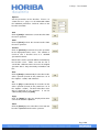
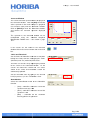
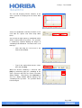
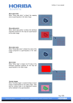
If the scan area has been set greater than the
maximum allowable dimensions a warning
message will be displayed.
This shows the
maximum negative and positive displacement
possible for the selected objective. The area size
set in the “Height” and “Width” boxes, or defined
according to the map pixel, or defined by the
rectangular video cursor, must not be greater than
the total displacement. In the example shown
right, the maximum displacement is -10 µm to
+10 µm, meaning a total displacement of 20 µm.
The
Raman
measurement
(spectrum
or
multidimensional spectral array) can now be set up
and acquired in the normal way. Remember that
the spectrum recorded will be an average
spectrum from the scanned area.
Click [Stop] to stop the DuoScan™ scanning
mirrors.
Page | 112
LabSpec 5 user manual
4.5.10.1.2. Point Mode
When DuoScan™ is used in Point Mode, it is
possible to move the laser spot to any position on
the sample surface, within the maximum possible
scan displacement. In this mode DuoScan™ can
be used as a substitute to the standard motorized
stage
for
point-by-point
XY
mapping
(multidimensional spectral array acquisition) – this
function is particularly useful when it is not possible
to move the sample underneath the laser beam, or
ultra-fine step size is required (down to
DuoScan™’s minimum step size of 50 nm).
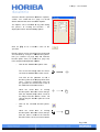
To use DuoScan™ in Point Mode the scanning
mirrors must be static. To confirm this, open the
DuoScan™ XY scanning dialog window by clicking
on the DuoScan icon.
If the DuoScan™ mirrors are scanning, the [STOP]
button will be active. Click on [STOP] to stop the
DuoScan™ scanning, and then click [CLOSE] to
close the dialog window.
Set the DuoScan™ module as the active XY stage
using the ‘switch stage’ icon in the XYZ Coord
section of the Control Panel (see section 9.10.2,
page 237).
The laser spot position can now be controlled by
inputting XYZ coordinates in the XYZ Coord
section of the Control Panel (see section 9.10,
page 236), or by acquiring a Raman XY map
(multidimensional spectral array) in the standard
way. In both cases, the laser spot is now moved
across the sample using the DuoScan™ mirrors.
The sample does not move.
Page | 113
LabSpec 5 user manual
4.6.
Data Processing and Analysis Icons
4.6.1.
Spectral ID Search
Launch the ‘one click’ Spectral ID database search for the active spectrum.
Clicking on this icon will initiate the following processes:
o
o
o
o
o
Export the active spectrum in Grams .spc format
Open Spectral ID
Load the exported spectrum into Spectral ID
Run a full spectrum matching search through the active databases
Report the list of matching spectra, with match quality scores
Please see the HORIBA Scientific manual “Using the Spectral ID Database Software with LabSpec 5”
and full documentation provided with the Spectral ID database software for more information about
Spectral ID and how it can be used and configured.
4.6.1.1.
Configuring LabSpec 5 for Correct Spectral ID Searching
The export procedure for the ‘one click’ Spectral ID search is defined by the options set in the File >
Save As dialog window for a Grams .spc file.
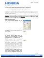
To ensure the ‘one click’ Spectral ID search performs correctly please complete the following set up
procedure in LabSpec 5:
o
o
o
o
o
Open a spectrum in any format
Click on File > Save As
Select “Grams (.spc)” from the “Save as
Type” drop down box
Tick the box for “Even spaced”
Click [Cancel]
If the “Even spaced” box is not ticked, the Spectral ID search will not be performed correctly, and
spurious results may be displayed.
Page | 114
LabSpec 5 user manual
4.6.2.
Baseline Correction
.....
Opens the Baseline dialog window.
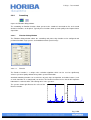
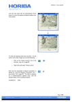
Baseline correction allows a high background in a spectrum to be subtracted, to yield a spectrum with
a flat, zero baseline. The correction can be applied to a single spectrum or a multidimensional
spectral array of spectra (including time profiles, Z (depth) profiles, temperature profiles, XY maps, XZ
and YZ slices, and XYZ datacubes).
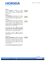
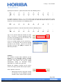
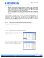
The example shown right illustrates a spectrum
before and after baseline correction.
4.6.2.1.
1 000
2 000
Raman Shift (cm-1)
3 000
1 000
2 000
Raman Shift (cm-1 )
3 000
Baseline Dialog Window
The Baseline dialog window allows the baseline correction to be configured and performed.
Page | 115
LabSpec 5 user manual
Options
Set the parameters for the baseline. Please see
section 4.6.2.1.1, page 117, for information about
the individual parameters and their affect on the
baseline correction.
Sub
Click on [Sub] to subtract the current baseline from
the active spectrum.
Clear
Click on [Clear] to clear the current baseline from
the active spectrum.
Convert
Click on [Convert] to convert the active spectrum
to the displayed baseline curve. This function is
useful to save a baseline curve in a standard
spectrum file format.
Note that the active spectrum will be overwritten by
the baseline curve. Make sure that the file is
saved with a different name to ensure the original
spectrum data is not permanently overwritten and
lost.
Auto
Click on [Auto] to automatically fit a baseline to the
active spectrum (based on the parameters set in
the “Options” section) and subtract it.
Fit
Click on [Fit] to automatically fit a baseline to the
active spectrum (based on the parameters set in
the “Options” section). The best fit baseline curve
will be displayed on the spectrum. It can be
subtracted by clicking on [Sub].
Copy
Click on [Copy] to copy the displayed baseline
curve to the baseline clipboard.
Paste
Click on [Paste] to paste a baseline curve from the
baseline clipboard onto the active spectrum.
Page | 116
LabSpec 5 user manual
4.6.2.1.1.
Baseline Correction Options
The Baseline options control the parameters of the baseline that will be used for baseline correction.
Type
Select the algorithm used to define the baseline
curve.
o
Polynom: fits a polynomial curve through
the baseline points set on the spectrum.
The degree of the polynomial is set in the
“Degree” drop down box.
o
Lines: fits a straight line between
baseline points set on the spectrum.
Degree
Select the degree of polynomial equation used to
create the baseline curve – this option is only used
when the baseline “Type” is set to “Polynom”.
In general the higher the degree the more
adaptable the baseline curve will be to strangely
shaped, non-uniform backgrounds.
Page | 117
LabSpec 5 user manual
Attach
Select the “Attach” mode for manual definition of
baseline points used to define the baseline curve.
o
No: baseline points are set at the exact
-1
intensity and spectral position (cm or
nm) specified by the user.
o
Yes: baseline points are forced to sit on
the spectrum, at the spectral position
-1
(cm or nm) specified by the user.
The “Attach” mode is particularly important when
defining a baseline to be used for correction of
multidimensional spectral array data. In this case,
“Attach” should be set to “Yes” to ensure that the
baseline points will adapt to the varying intensities
of the spectra within the multidimensional spectral
array.
Style
Set the display style of the baseline curve. The
colour, width and line style of the baseline curve
can be set using the “Style” drop down box.
4.6.2.2.
Setting a Baseline for Baseline Correction of a Single Spectrum
Select the spectrum which is to be baseline
corrected.
Click on the Baseline icon to open the Baseline
dialog window.
Page | 118
LabSpec 5 user manual
Select the baseline parameters within the “Options”
section. See section 4.6.2.1.1, page 117, for full
details about the Baseline Correction Options.
The options can be modified at any point during
the process of creating the baseline – the
displayed baseline will immediately update.
Click on [Fit] to fit a baseline curve to the
spectrum.
Baseline points can be manually inserted, adjusted
and removed by using the “Add baseline points”
icon (see section 5.14, page 180) and “Remove
baseline points” icon (see section 5.15, page 181)
in the Graphical Manipulation Toolbar.
o
Click on the “Add baseline points” icon.
The cursor will change from the mouse
cursor to the Add Baseline Points cursor.
Left click on the spectrum to add a
baseline point to the displayed baseline
curve. If there is no baseline curve on
the spectrum the first left mouse click in
this mode will create the baseline.
Hover the cursor over an existing
baseline point. When the cursor changes
from the Add Baseline Points cursor to
the Adjust Baseline Points cursor, left
click to drag the baseline point to a new
position.
o
Click on the “Remove baseline points”
icon.
Hover the cursor over an existing
baseline point. When the cursor changes
from the mouse cursor to the Remove
Baseline Points cursor, left click to delete
Page | 119
LabSpec 5 user manual
the baseline point from the baseline
curve.
The entire baseline can be cleared by
clicking on [Clear].
When the baseline curve is completed click [Sub]
to subtract it from the spectrum.
4.6.2.3.
Setting a Baseline for Baseline Correction of a Multidimensional Spectral Array
The procedure as outlined above (section 4.6.2.2, page 118) should be followed, but the baseline
curve should be created on the SpIm (spectral image) window.
In general it is useful to have the “Attach” mode set to “Yes” when applying a baseline to the SpIm
window, since this ensures the baseline points can adapt to the varying intensities typical in a
multidimensional spectral array.
Individual spectra within a multidimensional spectral array can be baseline corrected by applying the
correction to the individual spectrum displayed in the Point window.
When the baseline has been subtracted, ensure
the corrected spectrum is re-inserted into the
spectral array by clicking on the ‘blue arrow’ icon
displayed in the point window, or click [Correct] in
the Map Analysis dialog window (see section 4.6.9,
page 147).
This must be done before the
map/profile cursor is moved.
4.6.3.
Spectral Normalization and Correction
Opens the Correction dialog window.
The correction functions allow spectra to be normalized and zeroed, and for a substrate/contaminant
spectrum to be automatically subtracted.
4.6.3.1.
Correction Dialog Window
The Correction dialog window allows the user to apply spectral normalization and correction to both
single spectra, and multidimensional spectral arrays.
Page | 120
LabSpec 5 user manual
Normalize
Click on [Normalize] to normalize each spectrum
so that the total area, sum or maximum signal of
the spectrum is 100. If the “Limits” tick box is
ticked, the normalization will only be applied within
the displayed limits. In this case, the spectrum will
be normalized so that the area, sum, or maximum
signal within the limits is 100. The limits can be
adjusted by typing values in the “Limits” boxes, or
adjusting the cursor positions in the “Corrector”
window.
The normalization mode can be selected from the
“Normalization” section of the dialog window.
Zero
Click on [Zero] to automatically subtract a constant
intensity value from the active spectrum or
multidimensional spectral array, so that the lowest
intensity pixel is at zero. When applied to a
multidimensional spectral array, each spectrum in
the array is zeroed independently.
Get
Click on [Get] to load the active spectrum in the
main LabSpec 5 graphical user interface (GUI) into
the “Corrector” window.
Delete
Click on [Delete] to clear the “Corrector” window,
and remove the corrector spectrum displayed
there.
Page | 121
LabSpec 5 user manual
Subtract
Click on [Subtract] to subtract the corrector
spectrum (displayed in the “Corrector” window)
from the active spectrum or multidimensional
spectral array.
Multiply
Click on [Multiply] to multiply the active spectrum
or multidimensional spectral array by the corrector
spectrum (displayed in the “Corrector” window).
Correct
Click on [Correct] to correct the active spectrum or
multidimensional spectral array for the contribution
of the corrector spectrum (displayed in the
“Corrector” window). The intensity of the corrector
spectrum will be automatically adjusted before
subtraction to best fit the spectrum.
If the “Limits” tick box is ticked the corrector
intensity adjustment will be calculated only within
the displayed limits. The limits can be adjusted by
typing values in the “Limits” boxes, or adjusting the
cursor positions in the “Corrector” window.
This function is useful if a substrate, diluent or
contaminant spectrum needs to be removed from a
sample spectrum.
Threshold
Click on [Threshold] to threshold the active
multidimensional spectral array. The threshold
function will be applied to any spectra within the
array which has a maximum intensity (relative to
the most intensity spectrum in the array) less than
the displayed threshold value set in the “Limits and
Threshold” section.
The threshold function will convert the spectrum to
have zero intensity throughout its spectral range.
Page | 122
LabSpec 5 user manual
Corrector Window
The current corrector spectrum will be displayed in
the Corrector window. Click on [Get] to load the
active spectrum in the main LabSpec 5 graphical
user interface (GUI) into the “Corrector” window.
Click on [Delete] to clear the “Corrector” window,
and remove the corrector spectrum displayed
there.
The spectrum in the Corrector window can be
manipulated using the standard Graphical
Manipulation Toolbar icons – see section 5, page
164.
If the cursors are not visible in the Corrector
window click on the Center Cursors icon in the Icon
bar.
Limits and Threshold
Set the limits for Normalize and Correct functions
ticking the “Limits” tick box, and typing the “From”
(minimum) and “To” (maximum) limit values.
The limits can also be set by adjusting the position
of the cursors in the Corrector window. As the
cursors are moved the “From” and “To” values
shown in the “Limits and Threshold” section are
continuously updated.
Set the threshold value by typing in the desired
level (in percent, %) in the “Threshold %” box.
Normalization
Select the normalization mode for the Normalize
function.
o
o
o
{Sum} – normalize so that the sum of the
spectrum intensity is 100
{Area} – normalize so that the area of the
spectrum is 100
{Max} – normalize to the maximum
intensity point in the spectrum.
Page | 123
LabSpec 5 user manual
4.6.4.
Smoothing
Opens the Filtration dialog window.
The smoothing or filtration functions allow spectra to be smoothed, converted to first and second
derivative functions, or despiked. Typically these functions allow spectral quality to be improved after
acquisition.
4.6.4.1.
Filtration Dialog Window
The Filtration dialog window allows the smoothing and processing functions to be configured and
performed on both single spectra, and multidimensional spectral arrays.
4.6.4.1.1.
Denoise
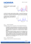
The Denoise function is a unique noise reduction algorithm which can be used to significantly
enhance spectrum quality without losing subtle spectral information.
Standard smoothing functions can result in loss of peak shape and position, and subtle features (such
as weak shoulders on a strong band) can be lost. The Denoise function ensures that all this important
information is retained, whilst still reducing noise in the spectrum.
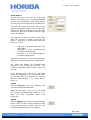
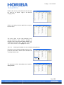
The spectra shown right illustrate the effect of the
Denoise function.
Page | 124
LabSpec 5 user manual
Two main Denoise algorithms are available from the “Denoise” drop down box:
o
o
Standard: recommended for spectra with signal to noise ≥ 20
Lite: recommended for very noisy spectra with signal to noise ≤ 20
In addition, both algorithms can be used with an integrated Despike function to remove random spikes
(also known as cosmic rays). See also section 3.5.4.7, page 37, for more information about other
spike filter options in LabSpec 5.
Note that the Denoise function can be automatically applied to all acquired
acquired data through the
Acquisition > Options dialog window – see section 3.5.4.15, page 46. If a spectrum has had the
Denoise function automatically applied through Acquisition > Options, it cannot have the function
applied again through the Filtration dialog window.
Using the Denoise Function
Select the desired Denoise algorithm from the
“Denoise” drop down box.
Click [Apply] to apply the Denoise algorithm to the
active spectrum.
4.6.4.1.2.
Matrix Operations
The functions described below require the
“Degree”, “Size”, and “Height” values to be set in
the drop down boxes, as described in the text.
Smooth
Click on [Smooth] to apply a Savitsky-Golay
smoothing function to the active spectrum.
Savitsky-Golay smoothing fits a polynomial
function of a specified “Degree” through a range
(“Size”) of adjacent pixels, and replaces those
pixels with the polynomial curve. The window
where this operation is applied is moved across the
entire spectrum. The “Degree” and “Size” must be
set to an appropriate level.
Typically the smaller the “Degree” and the larger
“Size” the more significant the smoothing. Note
that in some cases smoothing can remove or alter
Page | 125
LabSpec 5 user manual
features in a spectrum. Smoothing should be used
with care.
Der1
Click on [Der1] to convert the active spectrum to
its first derivative function. At each pixel position
the derivative is calculated using a defined range
(“Size”) of pixels either side of it.
Der2
Click on [Der2] to convert the active spectrum to
its second derivative function. At each pixel
position the second derivative is calculated using a
defined range (“Size”) of pixels either side of it.
Median
Click on [Median] to apply a non-linear median
smoothing function to the active spectrum.
Median smoothing replaces a spectrum pixel
intensity value by the median of intensity values
within a defined range (“Size”) either side of it.
This replacement process is repeated for all pixels
in the spectrum.
Typically the larger the “Size” the more significant
the median smoothing. Note that in some cases
median smoothing can remove or alter features in
a spectrum. Median smoothing should be used
with care.
Despike
Click on [Despike] to remove random spikes (also
known as cosmic rays) from a spectrum.
A spike is calculated as a pixel which has an
intensity greater than the average spectrum
intensity + “Height”.
The Despike function removes the spike and
replaces it with a weighted average of the
surrounding pixels.
Note that in some cases the Despike function can
remove or alter features in a spectrum, particularly
when the spectrum is comprised of very sharp
peaks. Despike should be used with care.
Please also see section 3.5.4.7, page 37, for more
information about other spike filter options in
LabSpec 5.
Page | 126
LabSpec 5 user manual
4.6.5.
Fourier Transform
Opens the Fourier Transform dialog window.
The Fourier Transform function allows smoothing of a spectrum based on direct Fourier data
transformation, applying filter and apodization functions. The spectrum is converted into its real and
imaginary Fourier functions, which essentially represents the spectrum as a combination of wave
patterns of varying frequency. Smoothing can be applied by removing high frequency contribution
(corresponding to noise) and leaving medium and low frequency contribution (corresponding to
Raman peaks).
The Fourier Transform smoothing function can be performed on both single spectra, and
multidimensional spectral arrays.
4.6.5.1.
Fourier Transform Dialog Window
The Fourier Transform dialog window displays the Fourier functions of the active spectrum, and
provides Apodization and Filter options for the transformation.
Fourier Data
The Fourier Data window displays the real and
imaginary Fourier functions of the active spectrum.
The red cursor can be used to set the high
frequency limit – frequencies above the limit
position will be removed from the spectrum.
Typically the lower the cursor position the more
smoothing is applied. At position 0 the spectrum is
fully smoothed (to a flat line). At position 100 the
spectrum is fully unsmoothed.
Page | 127
LabSpec 5 user manual
Limit
The Limit allows manual control of the “limit” cursor
displayed in the Fourier Data window. Type in the
required cursor position value (ranging between 0
and 100) and click on [Go].
Apod.
Select the type of apodization to be used in the
Fourier transformation from the “Apod.” drop down
box. The apodization reaches zero at the Limit
position.
Four modes are available:
o
o
o
o
No: no apodization
Line: linear apodization function
Sqrt: parabolic apodization function
Cos: cosine apodization function
Filter
Select whether a filter will be used for the Fourier
transformation, using the “Filter” drop down box.
Two modes are available:
o
o
No: no filter
Traffic: traffic filter
OK
Click [OK] to permanently apply the smoothing to
the active spectrum, and close the Fourier
Transform dialog window.
Cancel
Click [Cancel] to close the Fourier Transform
without applying the smoothing.
The original
spectrum will be left unchanged.
4.6.5.2.
Using the Fourier Tranform Function to Smooth a Spectrum
Select a spectrum to be smoothed.
Open the Fourier Transform dialog window by
clicking on the Fourier Transform icon in the Icon
Bar.
Page | 128
LabSpec 5 user manual
The real and imaginary Fourier functions of the
active spectrum are displayed in the Fourier Data
window.
Select the Apodization and Filter functions to be
used from the “Apod.” and “Filter” drop down
boxes.
Set the limit for high frequency contribution which
will be removed from the spectrum. The spectrum
is continuously updated allowing the degree of
smoothing to be monitored. The limit can be set in
two ways:
o
Click and drag the red cursor in the
Fourier Data window.
o
Type in the required limit into the “Limit”
box, and click [Go].
When the desired smoothing is achieved, click
[OK] to permanently apply the smoothing to the
active spectrum and close the Fourier Transform
dialog window. Alternatively click [Cancel] to
close the dialog window without applying any
smoothing to the spectrum. The spectrum will be
left unchanged.
Page | 129
LabSpec 5 user manual
4.6.6.
Math
Opens the Math dialog window.
Arithmetic functions can be applied to the intensity values of an active spectrum. Additionally, the
Extended Range spectral acquisition “Combine data” function can be applied post-acquisition through
the Math dialog window.
The Math functions can be performed on both single spectra, and multidimensional spectral arrays.
4.6.6.1.
Math Dialog Window
The Math dialog window contains text input boxes so that arithmetic functions can be created, and
then applied to the active data.
Const+
The “Const+” function adds a constant intensity
value to all pixels in the active spectrum.
Type in the desired constant, and click on the
adjacent [Go] button to apply the function to the
active spectrum. A positive constant will be added
to the spectrum intensity values; a negative
constant will be subtracted from the spectrum
intensity values.
Page | 130
LabSpec 5 user manual
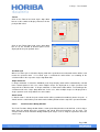
The example right shows the result of applying
“Const+”=1200 to a spectrum.
Intensity (cnt)
10 000
5 000
0
Intensity (cnt)
10 000
5 000
0
The “Const+” function can also be applied using
the “Add Constant” icon in the Graphical
Manipulation toolbar – see section 5.8, page 170.
Const*
The “Const*” function multiplies all pixel intensity
values in the active spectrum by a constant value.
Type in the desired constant, and click on the
adjacent [Go] button to apply the function to the
active spectrum. A constant greater than zero will
increase the spectrum intensity; whilst a constant
less than zero will decrease the spectrum intensity.
Page | 131
LabSpec 5 user manual
The example right shows the result of applying
“Const*”=2.5 to a spectrum.
10 000
Intensity (cnt)
8 000
6 000
4 000
2 000
0
10 000
Intensity (cnt)
8 000
6 000
4 000
2 000
0
The “Const*” function can also be applied using
the “Multiply by Constant” icon in the Graphical
Manipulation toolbar – see section 5.9, page 171.
Func 1 and Func 2
The “Func 1” and “Func 2” sections allow arithmetic functions to be created by the user, and applied
to the active spectrum.
The terminology used for these functions are as follows:
o
o
o
x and y refer to the intensity values of spectra which are open in LabSpec 5. x is the active
data file, and y is the other data file open in LabSpec 5. In the event that there is more than
one spectrum which could be used for y a message box will ask for the y spectrum to be
chosen from a list.
a, b and c refer to the values of the first, second and third axes of the active data file.
Standard arithmetic functions are also possible, including +, -, *, /, ^, exp, log, sin, asin,
cos, acos, tan, atan, abs, sqrt etc.
As an example, if “Func 1” = x + y, x refers to the intensity value at each pixel of the active spectrum,
and y refers to the intensity value at each pixel of another open spectrum. Assume the two spectra
have values as follows (where a represents the spectral axis):
a
x
y
1
10
1
2
12
2
3
15
3
4
25
2
5
22
1
6
13
1
7
10
4
8
7
3
...
...
...
Page | 132
LabSpec 5 user manual
applying the function x + y to this data will result in the following values:
a
x
y
1
11
1
2
14
2
3
18
3
4
27
2
5
23
1
6
14
1
7
14
4
8
10
3
...
...
...
As another example, if “Func 1” = x + 2*a, x refers to the intensity value of each pixel of the active
-1
spectrum, and a refers to the first axis (i.e., the spectral axis, with units Raman shift, cm ) value of
each pixel. Assume the data has the following values:
a
x
1
10
2
12
3
15
4
25
5
22
6
13
7
10
8
7
...
...
7
24
8
23
...
...
applying the function x + 2*a to this data will result in the following values:
a
x
1
12
2
16
3
21
4
33
5
32
6
25
Type in the desired arithmetic function for either
“Func 1” or “Func 2”, select the appropriate active
spectrum (corresponding to x in the function), and
click on the adjacent [Go] button.
If there are multiple options for the spectrum y, a
“Select Y” message box will ask for the desired
spectrum to be selected. Click on the desired
spectrum and then click [OK] to complete the
arithmetic procedure.
Combine
The “Combine” function allows individual spectral
windows in an Extended Range spectrum
acquisition to be glued together to yield a single
spectrum. This process can also be applied
automatically during an Extended Range
acquisition (see section 3.5.6, page 49).
Equally, the “Combine” function can be used to
create an average spectrum from all open spectra.
Set the options as desired:
o
Adjust intensity levels: if this box is ticked
the baselines of the individual spectral
windows will be adjusted prior to gluing,
Page | 133
LabSpec 5 user manual
o
to yield a seamless final spectrum. See
section 3.5.6.3, page 53, for full
information about this mode.
Remove combined datas: if this box is
ticked the individual spectra or spectral
windows
will
be
deleted
after
combination, leaving only the single
combined spectrum on screen.
Click on the adjacent [Go] button to apply the
“Combine” process.
4.6.7.
Peak Searching and Fitting
Opens the Peaks dialog window.
The Peak Searching and Fitting module allows peaks in a spectrum to be automatically labelled by
their position, and full peak fitting can be carried out to fully characterise peak parameters such as
position, amplitude, full width at half maximum height (FWHM) and area. Overlapping peaks can be
fully deconvoluted through the peak fitting routine.
The Peak Searching and Fitting functions can be performed on both single spectra, and
multidimensional spectral arrays.
4.6.7.1.
Peaks Dialog Window
The Peaks dialog window allows the peak searching, labelling and fitting processes to be configured
and applied, and displays the peak parameters after fitting.
Page | 134
LabSpec 5 user manual
Peak Options
Select the appropriate function to be used for peak
fitting from the “Function” drop down box. Three
default functions are provided:
o
o
o
Gaussian
Lorentzian
Mixed Gaussian-Lorentzian
Other functions can be defined by clicking on
[Functions...] in the Peaks dialog window – see
4.6.7.5, page 144, for full information.
If “Use area” is ticked the peak fitting routines will
also calculate the area of the peak(s). When “Use
area” is unticked only the default peak parameters
will be calculated.
These are peak position,
amplitude (i.e., maximum height), full width at half
maximum height (FWHM) and (for mixed
Gaussian-Lorentzian functions) the degree of
Gaussian contribution.
Search Options
Set the parameters used for automatic peak
searching and identification. The search routine
locates local intensity maxima, and assigns these
as peaks.
A local maximum must be greater than a certain
percentage of the maximum intensity in the whole
spectrum. The “Level (%)” parameter defines this
percentage of maximum spectral intensity.
Typically, as the “Level (%)” is increased, only the
most intense peaks will be identified. If low
intensity peaks need to be identified “Level (%)”
should be reduced.
A local maximum is assumed to exist within a finite
number of adjacent data points. The “Size (pnt)”
parameter defines this number. Typically, as the
“Size (pnt)” is increased, only peaks which are
widely separated will be identified. If close lying
peaks need to be identified “Size (pnt)” should be
reduced.
The “Level (%)” and “Size (pnt)” values can be set
by typing a value in the appropriate box, or using
the appropriate scroll bar. The peak labelling
displayed on the active spectrum will update
continuously, so that the result can be monitored.
Page | 135
LabSpec 5 user manual
Fitting Options
Set the parameters used for the peak fitting
routine. This routine uses a Levenberg-Marquardt
non-linear peak fit algorithm, and iteratively adjusts
all peak parameters to minimise the standard error.
The maximum number of iterations can be set by
typing an appropriate number in the “Iteration” box.
Typically the larger the iteration number the more
accurate the final fit result will be, but the longer
the process will take.
The algorithm can be set to miss out data points
within the spectrum, in order to speed up the
process. “Skip (pnt)” is used to define how many
points are missed.
o
o
o
“Skip (pnt)” = 0, all data points are used
for the fitting.
“Skip (pnt)” = 1, every second data point
is used for the fitting routine.
“Skip (pnt)” = 2, every third data point is
used for the fitting routine.
Typically as “Skip (pnt)” is increased the fit results
will be less accurate, but the process will be faster.
The “Error” box displays the Standard Error
between the fit result and the raw data. The
smaller the Standard Error the more accurate the
fit result.
If the “Baseline” box is ticked the peak fitting
routine will additionally fit the specified baseline.
The baseline must be specified first, using the
Baseline dialog window – see section 4.6.2.1,
page 115.
Search
Click on [Search] to start the automatic peak
searching and identification routine.
Adjust the “Size (pnt)” and “Level (%)” to control
the searching and identification procedure – see
above for more information about these
parameters.
Approx
Click on [Approx] to run the peak approximation
routine, which can be used to estimate the initial
peak parameters prior to fitting. Only the peak
position and width parameters are adjusted.
Page | 136
LabSpec 5 user manual
The peak approximation is a useful function to
assist in complex peak fitting procedures. Running
the peak approximation routine prior to full fitting
ensures that the starting parameters are realistic
and close to their true values. This reduces the
possibility of the peak fitting routine locating an
incorrect solution.
Fit
Click on [Fit] to run the peak fitting routine, which
can be used to calculate peak position, amplitude,
full width at half maximum height (FWHM),
Gaussian contribution and area.
The peak fitting routine can only be used if peaks
have been located in the spectrum. Peaks can be
located automatically using the [Search] button, or
manually by using the “Add peak” icon in the
Graphical Manipulation toolbar (see section 5.10,
page 172).
Init
Click on [Init] to restore peak parameters in the
SpIm window of a multidimensional spectral array
to the initial values before the peak approximation
[Approx] or fitting [Fit] routines were run.
Clear
Click on [Clear] to clear all peaks from the active
spectrum.
Convert
Click on [Convert] to convert the active spectrum
to the sum of the displayed peaks. This function is
useful to save a theoretical peak fit solution in a
standard spectrum file format.
Note that the active spectrum will be overwritten by
the sum of the displayed peaks. Make sure that
the file is saved with a different name to ensure the
original spectrum data is not permanently
overwritten and lost.
Peaks...
Click on [Peaks...] to open the Peak Parameters
dialog window, to view and manually set peak
position, amplitude, full width at half maximum
height (FWHM), Gaussian contribution and area
values for all peaks labelled on a spectrum.
Page | 137
LabSpec 5 user manual
See section
information.
4.6.7.2,
page
138,
for
more
Variables...
Click on [Variables...] to open the Peak Variables
dialog window, to view and set initial values and
maximum/minimum values for variables within the
peak fitting routine.
See section
information.
4.6.7.3,
page
140
for
more
Options...
Click on [Options...] to open the Peak Options
dialog window, to view and set display options for
the peak labelling and fitting.
See section
information.
4.6.7.4,
page
143,
for
more
Functions...
Click on [Functions...] to open the Peak Functions
dialog window, to view and create user defined
peak shape functions.
See page 4.6.7.5, page 144, for more information.
4.6.7.2.
Peak Parameters Dialog Window
The Peak Parameters dialog window displays peak position, amplitude, full width at half maximum
height (FWHM), Gaussian contribution and area for all peaks labelled on a spectrum. The
parameters can be manually adjusted and fixed so that the parameter is not varied during the fitting
routine.
The Peak Parameters dialog window for individual spectra (e.g., Spectrum window, or Point window
of a multidimensional spectral array) has the following appearance:
The Peak Parameters dialog window for multidimensional spectral arrays (e.g., the SpIm window of a
multidimensional spectral array) has the following appearance:
Page | 138
LabSpec 5 user manual
Each row displays the parameters for a single peak:
o
o
o
o
o
o
o
o
p – peak position, in units as displayed on the spectrum’s X axis, typically Raman shift
-1
(cm ) or nanometers (nm).
a – peak amplitude, in units as displayed on the spectrum’s Y axis, typically counts (cnt), or
counts per second (cnt/s).
w – peak full width at half maximum height (FWHM) in units as displayed on the spectrum’s
-1
X axis, typically Raman shift (cm ) or nanometers (nm).
g – Gaussian contribution in a mixed Gaussian-Lorentzian function. The value of Gaussian
contribution varies from 0 (no Gaussian contribution, fully Lorentzian) through to 1 (fully
Gaussian). The g column is only displayed when a mixed Gaussian-Lorentzian function is
selected for peak fitting in the main Peaks dialog window (see section 4.6.7.1, page 134).
Formula – the function used for the peak fitting, as selected in the main Peaks dialog
window (see section 4.6.7.1, page 134). “Gauss()” = Gaussian, “Loren()” = Lorentzian,
“GaussLoren()” = mixed Gaussian-Lorentzian.
Area – the area of the peak, in area units based on the units displayed on the spectrum’s X
and Y axes. The Area column is only displayed if the “Use area” box is ticked in the main
Peaks dialog window (see section 4.6.7.1, page 134).
Fix - the “Fix” tick boxes to the right of each of the p, a, w and g parameters allows a
parameter to be fixed. A fixed parameter will not be varied during the peak fitting routine.
When a box is ticked the parameter is fixed. When a box is unticked the parameter will be
varied during the fitting routine.
Map – the “Map” tick boxes (which are only displayed for the SpIm window of a
multidimensional spectral array) to the right of each of the p, a, w, g and Area parameters
allows a profile or map image to be generated based on the parameter. For example, it is
possible to create an image based on peak position, illustrating how the peak position varies
across the map area. To display a profile/image based on a peak parameter tick the
appropriate box and click [Apply]. A new map profile/image will be created. To close the
map profile/image, untick the box and click [Apply].
Copy
Click on [Copy] to copy the parameters displayed
in the Peak Parameters dialog window.
Parameters which have been copied can be
pasted into other programmes (such as Microsoft
Office) or into the Peak Parameters dialog window.
This function can be used to copy peak parameters
from one spectrum and paste them to another
spectrum (using [Paste]).
Page | 139
LabSpec 5 user manual
Paste
Click on [Paste] to paste parameters in the Peak
Parameters dialog window.
This function can be used to paste peak
parameters copied (using [Copy]) from one
spectrum to another.
Apply
Click on [Apply] to update the peak(s) displayed
on the spectrum according to parameters in the
Peak Parameters dialog window.
This button must be used when parameters are
manually adjusted in the Peak Parameters dialog
window. The peaks displayed on the spectrum will
not reflect the new parameters until [Apply] is
clicked.
4.6.7.3.
Peak Variables Dialog Window
The Variables dialog window displays the initial parameters used in the peak fitting procedure, and
the minimum and maximum values they can take during the fitting procedure. In most cases the
default values are suitable for general peak fitting routines, but in specific cases the initial parameters
and their minimum and maximum values can be manually adjusted as required.
The Variables dialog shows the initial (“init”) values, and minimum (“Min”) / maximum (“Max”) values
for each parameter:
o
o
o
p – peak position, in units as displayed on the spectrum’s X axis, typically Raman shift
-1
(cm ) or nanometers (nm). In the example shown above, the initial value of p is the X axis
position (“x”) at which the peak is initially located or positioned, and the position can be
varied from p-5 to p+5 during the fitting procedure.
w – peak full width at half maximum height, in units as displayed on the spectrum’s X axis,
-1
typically Raman shift (cm ) or nanometers (nm). In the example shown above, the initial
value of w is 3, and width can be varied from 0.001 to 200 during the fitting procedure.
a – peak amplitude, in units as displayed on the spectrum’s Y axis, typically counts (cnt), or
counts per second (cnt/s). In the example shown above, the initial value of a is the Y axis
position (“y”) at which the peak is initially located or positioned, and the amplitude can be
varied from 0 to the maximum Y axis value (“maxy”) during the fitting procedure.
Page | 140
LabSpec 5 user manual
o
o
b, c, d – parameters within the Gaussian/Lorentzian equations. In the example shown
above, the initial values of b, c and d are 0, and they can be varied from either the inverse
of the maximum Y axis value (“-maxy”) or the minimum Y axis value (“miny”), to the
maximum Y axis value (“maxy”) during the fitting procedure.
g – Gaussian contribution in a mixed Gaussian-Lorentzian function. In the example shown
above, the initial value of g is 0.5, and the Gaussian contribution can be varied from 0 (no
Gaussian contribution, fully Lorentzian) through to 1 (fully Gaussian) during the fitting
procedure.
If “Copy” is ticked for a parameter the “min” and “max” values will be displayed individually for each
peak in the Peak Parameters dialog window. This allows “min” and “max” parameters to be set
individually for each peak. Note that the “Copy” box must be ticked before the peaks are
automatically located using [Search] or manually located using the “Add peak” icon in the Graphical
Manipulation toolbar (see section 5.10, page 172).
4.6.7.3.1.
Setting the Init, Min and Max Values in the Variables Dialog Window
Window
Left click in the desired parameter “init”, “min” or “max” box and insert the desired value.
information for each parameter as required.
4.6.7.3.2.
Add
Adding Parameters to the Variables Dialog Window
Additional categories can be added by right
clicking on one of the parameter name boxes and
selecting “Insert row”.
A new row will be inserted above the selected
position, and will display the same name and “init”,
“min” and “max” values as the original parameter.
Page | 141
LabSpec 5 user manual
Double click on the parameter name box to allow
the name to be edited. Type in the desired
category name.
Click on any other parameter name box to register
the new name.
The name given to the new parameter must
exactly match the name used in definition of
functions in the Peak Functions dalog window (see
section 4.6.7.5, page 144). The “init”, “min” and
“max” values must be set to appropriate values.
4.6.7.3.3.
Deleting Parameters from the Variables Dialog Window
Parameters can be deleted by right clicking on the
parameter name boxes which is to be deleted and
selecting “Remove row”.
The parameter will be deleted from the Variables
dialog window.
Page | 142
LabSpec 5 user manual
4.6.7.4.
Peak Options Dialog Window
The Peak Options dialog window allows control of the display options for the peak labelling and fitting.
The following peak labelling and fitting display components can be controlled:
Text
Click on the Text “Style” drop down box to set the font, font style, font size and font color used to
display the peak position on the spectrum. If “Show” is ticked the peak position will be displayed on
the spectrum. Note that if “Use data style” is ticked the colour will be set to match the spectrum color.
If “Use data style” is unticked the colour will be set according to the selection made in the “Style” drop
down box.
Arrow
Click on the Arrow “Style” drop down box to set the colour, width and line style for the arrow marker
indicating the peak position. If “Show” is ticked the arrow marker will be displayed on the spectrum.
Note that if “Use data style” is ticked the colour will be set to match the spectrum color. If “Use data
style” is unticked the colour will be set according to the selection made in the “Style” drop down box.
Shape
Click on the Shape “Style” drop down box to set the colour, width and line style for the individual peak
shape(s) displayed on the spectrum. If “Show” is ticked the peak shape(s) will be displayed on the
spectrum. Note that if “Shape multicolor” is ticked the colour will be automatically selected from a
default palette; in this case, when multiple shapes are displayed on a single spectrum each shape will
be a different color. If “Shape multicolor” is unticked the colour will be set according to the selection
made in the “Style” drop down box; in this case, when multiple shapes are displayed on a single
spectrum each shape will be the same colour.
Sum
Click on the Sum “Style” drop down box to set the colour, width and line style for the sum spectrum
(i.e., the combination spectrum created by summing all the peak shapes displayed). If “Show” is
ticked the sum spectrum will be displayed on the spectrum.
Residual
Click on the Residual “Style” drop down box to set the colour, width and line style for the residual
spectrum (i.e., the difference between the sum spectrum and the raw data). If “Show” is ticked the
residual spectrum will be displayed on the spectrum.
Page | 143
LabSpec 5 user manual
Format
Click on the Format left hand “Style” drop down
box to set the number of display characters for the
peak position value.
Click on the Format right hand “Style” drop down
box to set the number of decimal places to be
displayed for the peak position value.
Use data style
When “Use data style” is ticked the display color of the peak label text and arrow marker will be set to
match the spectrum color. If “Use data style” is unticked the color will be set according to the
selection made in the respective “Style” drop down box.
Shape multicolor
If “Shape multicolor” is ticked the individual peak shape display colour will be automatically selected
from a default palette; in this case, when multiple shapes are displayed on a single spectrum each
shape will be a different color. If “Shape multicolor” is unticked the colour will be set according to the
selection made in the “Style” drop down box; in this case, when multiple shapes are displayed on a
single spectrum each shape will be the same colour.
Attach arrow
If “Attach arrow” is ticked the peak arrow marker will be positioned immediately above the peak. If
“Attach arrow” is unticked the peak arrow marker will be positioned at the top of the spectrum window.
4.6.7.5.
Peak Functions Dialog Window
The Peak Functions dialog window allows custom peak fitting formulae to be defined, so that shapes
other than the default Gaussian, Lorentzian and mixed Gaussian-Lorentzian can be used. For
example, with the Peak Functions dialog window peak shapes such as Voigt or asymmetric Gaussian
can be used.
Page | 144
LabSpec 5 user manual
To define a custom peak shape formula type the shape name in a “Name” text box, and input the
formula in the “Formula” text box. The name will be displayed in the main “Functions” drop down box
in the main Peaks dialog window.
Any parameter can be used, but it must also be defined as a parameter in the Peak Variables dialog
window (see section 4.6.7.3, page 140). Note that certain parameters are predefined:
o
o
o
4.6.8.
p – peak position, in units as displayed on the spectrum’s X axis, typically Raman shift
-1
(cm ) or nanometers (nm).
a – peak amplitude, in units as displayed on the spectrum’s Y axis, typically counts (cnt), or
counts per second (cnt/s).
w – peak full width at half maximum height (FWHM) in units as displayed on the spectrum’s
-1
X axis, typically Raman shift (cm ) or nanometers (nm).
Profile
Opens the Profile dialog window.
The Profile dialog window displays an intensity profile across an image (such as optical image, or two
dimensional Raman mapped image).
Page | 145
LabSpec 5 user manual
Profile
The “Profile” window displays the image intensity
profile at the cursor position. The scales for the X
and Y axes are taken directly from the image itself.
The profile is created in either a horizontal (X axis)
or vertical (Y axis) direction in the image,
depending on the selection made in the drop down
box:
o
o
Hor – horizontal (X axis)
Ver – vertical (Y axis)
Corr
Click on [Corr] to modify the image based on
manipulation made to the profile. For example, if
the profile displayed in the Profile dialog window is
smoothed, clicking on [Corr] will apply the same
smoothing function to the entire image in the
horizontal or vertical dimensions (according to the
selection of “Hor” or “Ver” in the drop down box).
4.6.8.1.
Displaying an Intensity Profile from an Image
To display an intensity profile from an image (such
as optical image, or two dimensional Raman
mapped image) open the image file.
In the case of a two dimensional Raman mapped
image click on the image window (either “Map” or
“Score”). Select the component from which the
profile is to be created, using the tags in the right
hand Data bar (see section 6.3, page 198).
Ensure the cursor mode in the image window is set
to “Cross” (right click and select “Cursor”, and then
choose “Cross” from the Style drop down box).
Open the Profile dialog window by clicking on the
Profile icon in the Icon bar.
Position the cursor at the point of the image from
where the profile is to be created.
Page | 146
LabSpec 5 user manual
Select “Hor” or “Ver” from the drop down box in the
Profile dialog window to create an intensity profile
in the horizontal (X axis) direction or vertical (Y
axis) direction respectively.
The profile is displayed in the Profile dialog
window. Standard data processing functions (such
as smoothing, peak fitting or baselining) and
copy/paste functions can be used with this profile.
Click [Close] to close the Profile dialog window.
4.6.9.
Map Analysis
Opens the Map Analysis dialog window.
The Map Analysis dialog window displays the positions and settings for the “Red”, “Green” and “Blue”
cursors which are used to create intensity profiles and images from multidimensional spectral arrays
(including time profiles, Z (depth) profiles, temperature profiles, XY maps, XZ and YZ slices, and XYZ
datacubes). The positions and settings can also be manually configured in this dialog window.
Use
If the “Use” box is ticked for a set of cursors (“Red”, “Green” or “Blue”) then a profile or image will be
generated displaying the average intensity between the two cursors. The cursor positions are set by
clicking the “Red”, “Green” or “Blue” cursor icons in the left hand Graphical Manipulation bar (see
section 5.2, page 165) and dragging the cursors to the desired positions on either the “SpIm” or
“Point” windows, or by typing in desired values into the “From” and “To” boxes in the Map Analysis
dialog window.
Note that if “Use” is unticked for all three cursors and “Green/Blue” is also unticked, the “Map” window
will not be displayed. To redisplay the “Map” window make sure that at least one of the “Use” boxes
are ticked, or that the “Green/Blue” box is ticked.
Page | 147
LabSpec 5 user manual
Baseline
If the “Baseline” box is ticked for a set of cursors (“Red”, “Green” or “Blue”) then the cursor region is
first baselined before calculation of the average intensity between the cursors. This mode is useful to
ensure that the image created truly reflects peak intensity and not general background intensity
(perhaps from fluorescence or photoluminescence).
From and To
Displays the beginning (“From”) and end (“To”) spectral positions for a set of cursors (“Red”, “Green”
or “Blue”). These can be manually adjusted by typing in desired values and clicking [OK].
Green/Blue
If the “Green/Blue” box is ticked an additional profile/image is displayed, showing the ratio of average
intensities of the “Green” and “Blue” cursors (i.e., [IntensityGREEN] / [IntensityBLUE]). This display is
useful to visualize a change in peak ratios within a multidimensional spectral array.
To remove the “Green/Blue” intensity profile/image untick the box.
Spectrum
If the “Spectrum” box is ticked the “Point” window is displayed, showing the spectrum at the current
cursor position.
Note that if the “Spectrum” box is unticked, the “Point” window will not be displayed. To redisplay the
“Point” window tick the “Spectrum” box.
In the event that the “Point” window is accidentally deleted within the main LabSpec 5 graphical user
interface (GUI), use the following procedure to re-display the window:
o
o
o
o
o
o
o
open the Map Analysis dialog window
untick the “Spectrum” box
click [OK]
re-open the Map Analysis dialog window
tick the “Spectrum” box
click [OK]
the Point window is now displayed in the main LabSpec 5 graphical user interface (GUI)
Correct
Click on [Correct] to update the multidimensional
spectral array with the “Point” spectrum after it has
been processed/modified in some way (for
example, smoothing or baselining).
The “Point” window only displays data held within
the multidimensional spectral array, so if the
spectrum in the “Point” window is modified it is
necessary to update the actual data in the array by
clicking on [Correct]. If this is not done, when the
cursor on the profile/image is moved the
modifications will be lost – the next time the
spectrum is displayed in the “Point” window it will
return to its original form.
Page | 148