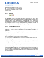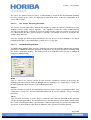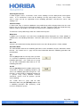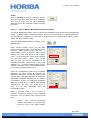
Download LabSpec 5 user manual Page | 149 4.6.10. Create

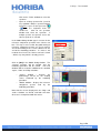
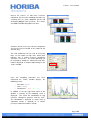
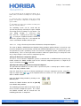
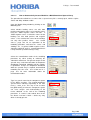
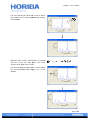
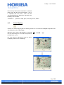
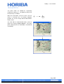
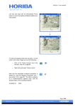
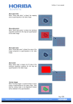
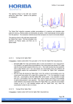
LabSpec 5 user manual
Load
Click on [Load] to load a cursor parameters file (in
.ngp format) so that a previously saved
configuration of the Map Analysis dialog window
can be recalled and applied.
Save
Click on [Save] to save a cursor parameters file (in
.ngp format) so that the current configuration of the
Map Analysis dialog window can be saved, and
recalled at any time.
Convert
Click on [Convert] to convert an existing image file
into the LabSpec 5 multidimensional spectral array
format, including “SpIm”, “Point” and “Map”
windows.
4.6.10.
Create Spectral Profile
Opens the Spectral Profile dialog window.
The Spectral Profile dialog window allows a 1D multidimensional spectral array to be created from
individual spectra, and for spectra to be added to, deleted from, and inserted into an existing 1D
multidimensional spectral array. This function is useful to create profiles from spectra where there is
sequential change in some experimental parameter (e.g., reaction temperature, or concentration).
Name
Type the desired name for a new profile in the
“Name” text box before clicking on [New] to create
the profile.
New
Click on [New] to create a new spectral profile,
using the active spectrum as the first spectrum in
the profile.
Page | 149
LabSpec 5 user manual
If the “Multi” function is active (see section 3.4.2,
page 23) then all open spectra will be added to the
spectral profile when it is created. In this case, the
active spectrum will be added first, followed by all
other open spectra in the order they appear within
the right hand Data bar.
See section 4.6.10.1, page 151, for further
information.
Add
Click on [Add] to add the active spectrum to the
end of the spectral profile.
See section 4.6.10.2, page 152, for further
information.
Insert
Click on [Insert] to add the active spectrum to the
spectral profile at the position shown by the cursor
in the “Map” window.
See section 4.6.10.3, page 152, for further
information.
Delete
Click on [Delete] to delete a spectrum from the
spectral profile. The spectrum at the position
shown by the cursor in the “Map” window will be
deleted.
See section 4.6.10.4, page 153, for further
information.
XYZ
Click on [XYZ] to rotate an XYZ multidimensional
spectral array so that the data is formatted in the
default Z.Y.X format (e.g., a Z-stack of YX maps).
See section 4.5.5.3, page 99, for information about
controlling
the
acquisition
order
for
multidimensional spectral arrays.
Page | 150
LabSpec 5 user manual
4.6.10.1.
Creating a New Spectral Profile
Using File > Open menu, or the Open icon (
/
) open the individual spectra which are to be
used to create the spectral profile.
Open the Spectral Profile dialog window by clicking
on the Create Spectral Profile icon.
Type into the “Name” text box a name for the new
profile.
Select the first spectrum to be added to position 1
in the new profile, and click [New] to create the
profile. The new profile will be created in two
ways, depending whether the “Multi” function is
active (see section 3.4.2, page 23):
o
o
“Multi” active: the active spectrum will be
added to position 1 in the profile, followed
by all other open spectra, in the order
they appear within the right hand Data
bar.
“Multi” inactive: the active spectrum will
be added to position 1 in the profile. No
other spectra will be added to the profile.
Additional spectra can be added to the
profile using the [Add] button (see
section 4.6.10.2, page 152) or [Insert]
button (see section 4.6.10.3, page 152).
When the profile is created, the standard “SpIm”,
“Point” and “Map” windows associated with a
multidimensional spectral array will be displayed.
The profile can now be analysed in the normal
way, using cursors and modelling.
Page | 151
LabSpec 5 user manual
The profile will be created with each spectrum
assigned to an integer value on the X axis, and the
X axis label is set to “Points”. To modify the
scaling and axis label use the Data Range dialog
window, accessed through the Data > Data Range
menu, the Data Range icon (
/
), or by using
the keyboard short cut <CTRL>+D. See section
3.3.2, page 20, for more information about the
Data Range dialog window.
Save the spectral profile (in .ngc format) by
activating the “SpIm” window and using the File >
Save As menu, or the Save icon (
4.6.10.2.
/
).
Adding Spectra to a Spectral Profile
To add a spectrum into an existing Spectral Profile,
use File > Open menu, or the Open icon (
/
), or the keyboard short cut <CTRL>+O to
open the spectrum which is to be added.
Select the spectrum, and click on [Add] to
automatically add the spectrum at the end of the
spectral profile. For example, if the profile already
has spectra at positions 1, 2 and 3, a new
spectrum added to the profile will be at position 4.
4.6.10.3.
Inserting Spectra into a Spectral Profile
To insert a spectrum into an existing Spectral
Profile, use File > Open menu, or the Open on
(
/
), or the keyboard short cut <CTRL>+O
to open the spectrum which is to be inserted.
In the profile “Map” window, activate the cursor and
select the position at which the new spectrum is to
be inserted.
Select the spectrum which is to be inserted, and
click on [Insert] to insert it at the position indicated
by the cursor.
In a default spectral profile, the other spectra
originally at and above this position will be shifted
Page | 152
LabSpec 5 user manual
upwards in the profile. For example, if spectra A, B
and C are currently at positions 1, 2 and 3 in a
profile of form 1A, 2B, 3C, when spectrum D is
inserted at position 2, the new profile will take the
form 1A, 2D, 3B, 4C.
In a spectral profile where the scale has been
manually modified using the Data Range dialog
window (see section 3.3.2, page 20), the first and
last positions of the profile will remain fixed. The
positions of spectra within the profile will be
adjusted when a spectrum is inserted.
For
example, if spectra A, B and C are currently at
positions 1, 2 and 3 in a manually scaled profile of
form 1A, 2B, 3C, when spectrum D is inserted at
position 2, the new profile will take the form 1A,
1.66D, 2.33B, 3C. If necessary the profile can be
rescaled using the Data Range dialog window after
the spectrum has been inserted.
4.6.10.4.
Deleting Spectra from a Spectral Profile
In the profile “Map” window, activate the cursor and
select the position from which a spectrum is to be
deleted.
Click on [Delete] to delete the spectrum from the
position indicated by the cursor position.
In a default spectral profile, the other spectra
above this position will be shifted downwards in the
profile. For example, if spectra A, B, C and D are
currently at positions 1, 2, 3 and 4 in a profile of
form 1A, 2B, 3C, 4D, when spectrum B is deleted,
the new profile will take the form 1A, 2C, 3D.
In a spectral profile where the scale has been
manually modified using the Data Range dialog
window (see section 3.3.2, page 20), the first and
last positions of the profile will remain fixed. The
positions of spectra within the profile will be
adjusted when a spectrum is deleted.
For
example, if spectra A, B, C and D are currently at
positions 1, 2, 3 and 4 in a manually scaled profile
of form 1A, 2B, 3C, 4D when spectrum B is
Page | 153
LabSpec 5 user manual
deleted, the new profile will take the form 1A, 2.5C,
4D. If necessary the profile can be rescaled using
the Data Range dialog window after the spectrum
has been deleted.
4.6.11.
Modelling
Opens the Model dialog window.
The Model dialog window is used to set up and perform a direct classical least squares (DCLS)
modelling procedure on multidimensional spectral arrays (including time profiles, Z (depth) profiles,
temperature profiles, XY maps, XZ and YZ slices, and XYZ datacubes) using a set of reference
component spectra. This procedure is used to identify the distribution of the reference component
spectra within the spectral array to create a profile/image based on the component distribution. The
component spectra can be either manually selected (from previously saved spectra, or from within the
spectral array) or automatically created by LabSpec 5 using a clustering algorithm.
4.6.11.1.
The DCLS Modelling Procedure
At each position within the multidimensional spectral array the DCLS modelling procedure finds a
linear combination of the reference component spectra which best fits the raw data. The resulting
profile/image is created by showing the contribution (‘score’) of each component (‘loading’) as a
profile/image.
For example, if there are three loadings (A, B, and C) with scores (x, y and z) the sum, S, of the linear
combination is represented by:
S=[x*A]+[y*B]+[z*C]
A, B, C are the loadings, e.g., reference spectra of pure components.
x, y, z are the scores, e.g., the ‘amount’ of each loading necessary so that S matches the raw data.
Normalized Modelling
When the modelling procedure is normalized (i.e., the “Normalize” box is ticked prior to performing the
modelling procedure), the reference component spectra (loadings) are normalized before the
modelling procedure takes place.
The scores are normalized so that the combination of all scores adds to 100%. If normalization is
turned off after normalized modelling has been performed, the scores are shown as their true values.
Unnormalized Modelling
When the modelling procedure is unnormalized (i.e., the “Normalize” box is unticked prior to
performing the modelling procedure), the reference component spectra (loadings) are used with their
raw intensities during the modelling procedure. Unnormalized modelling must be used if quantitative
analysis is required, since the actual intensity of each reference component spectrum relates directly
to the its concentration.
Page | 154
LabSpec 5 user manual
The scores are shown as their true values. If normalization is turned on after unnormalized modelling
has been performed, the scores are displayed as normalized values so that the combination of all
scores adds to 100%.
4.6.11.2.
The “Create” Clustering Procedure
The “Create” clustering procedure automatically identifies a number of reference component spectra
(loadings) using a factor analysis algorithm. This algorithm searches the entire multidimensional
spectral array and locates a number of clusters of similar spectra, where the average of each cluster
is as different from the other cluster averages as possible. The number of clusters is specified in the
“Factors” drop down box.
Once the average spectra have been identified in this way they are used as loadings in the DCLS
modelling procedure, as described above (section 4.6.11.1, page 154).
4.6.11.3.
The Model Dialog Window
The Model dialog window allows reference component spectra to be manually added to the modelling
procedure, in addition to automatic generation of component spectra with subsequent modelling using
the “Create” clustering procedure. The display mode of the modelling result can also be configured
through the dialog window.
Name
Type in a name in the “Name” text box for each reference component spectrum to be used in the
modelling procedure, prior to clicking on [Get] to start the modelling. See section 4.6.11.4, page 157,
for more information about how to use the modelling procedure.
Factors
Select the number of factors to be automatically created using the “Create” clustering procedure. See
section 4.6.11.5, page 161, for more information about how to use the automatic “Create” clustering
procedure.
Thr(%)
Type in a value (in percent, %) in the “Thr(%)” text box to set the intensity threshold for the automatic
“Create” clustering procedure. The threshold ensures that low intensity spectra will be excluded from
the “Create” clustering procedure – spectra with a maximum signal level less than the threshold value
(in percent, %) of the highest signal intensity within the entire spectra array will be ignored.
Page | 155
LabSpec 5 user manual
Allow Negative Scores
If “Allow negative scores” is ticked the scores for the loadings can take both positive and negative
values. If it is unticked the scores for the loadings can only take positive values. See section
4.6.11.1, page 154, for an explanation of the modelling procedure, and what the ‘scores’ and
‘loadings’ are.
Show Error Map
If “Show error map” is ticked an additional score profile/image will be displayed based on the error
between the sum of the linear combination and the raw data. Regions of high error (bright intensity)
indicate a bad fit, and could be caused by a missing reference component spectrum.
To remove the error profile/image untick the “Show error map” box.
Model Sum
If “Model sum” is ticked the sum of the linear combination will be displayed in the “Point” window, in
addition to the score/loading information. Select the colour for the sum spectrum from the drop down
box.
Error Text
Select the text colour from the drop down box for the error value displayed in the “Point” window.
Normalize Model
The normalization mode for the modelling procedure can be controlled using the “Normalize model”
tick box. See section 4.6.11.1, page 154, for more information about the modelling procedure and
normalization.
Get
Click on [Get] to load the currently active spectrum
as a reference component spectrum and start the
modelling procedure. See section 4.6.11.4, page
157, for more information about how to use the
modelling procedure.
Get All
Click on [Get All] to load in multiple model spectra
saved from a previous modelling procedure, and
start a new modelling procedure using them. This
function is useful to apply a modelling procedure to
a spectral array using identical reference
component spectra used for previous spectral
array modelling.
See section 4.6.11.4.1, page 160, for more
information about using the [Get All] button to start
a modelling procedure with previously saved
reference component spectra.
Page | 156
LabSpec 5 user manual
Create
Click on [Create] to
clustering procedure
See 4.6.11.5, page
about how to use the
procedure
4.6.11.4.
start the automatic “Create”
and subsequent modelling.
161, for more information
automatic “Create” clustering
How to Model a Multidimensional Spectral Array
The DCLS modelling procedure can be used with any multidimensional spectral array (including time
profiles, Z (depth) profiles, temperature profiles, XY maps, XZ and YZ slices, and XYZ datacubes).
The procedure described here assumes that a spectral array file is currently open, with the “SpIm”,
“Point” and “Map” windows visible.
Open the Model dialog window by clicking on the
Modelling icon.
Select whether loading scores can take both
positive and negative values, or just positive values
using the “Allow negative scores” tick box. If
“Allow negative scores” is ticked the scores for the
loadings can take both positive and negative
values. If it is unticked the scores for the loadings
can only take positive values.
See section
4.6.11.1, page 154, for an explanation of the
modelling procedure, and what the ‘scores’ and
‘loadings’ are. In general “Allow negative scores”
should be unticked, and it is recommended that it
is ticked for specialized analysis only.
Select the normalization mode of the modelling
procedure, by either ticking or unticking the
“Normalize model” box. For general analysis of the
spectral array, and characterisation of component
distribution normalized modelling will be suitable.
If quantitative analysis of component distribution
within the spectral array is required, unnormalized
modelling must be used. See section 4.6.11.1,
page 154, for more information about the
normalization modes.
Select a spectrum which is to be used as a
reference component spectrum in the modelling
procedure. The spectrum can be selected in two
ways:
o
Locate a ‘pure’ reference component
spectrum from within the spectral array
using the cursor in the “Map” window.
Page | 157
LabSpec 5 user manual
o
Click on the “Point” window to select the
spectrum.
Open an existing spectrum file (saved in
any standard LabSpec spectrum format)
using File > Open, or the Open icon (
/
), or the keyboard short cut
<CTRL>+O.
Click on the spectrum
window and select the spectrum. If
multiple spectra are opened, ensure the
correct spectrum is selected.
In the Model dialog window type in a name for the
reference component spectrum in the “Name” text
box. This step is not essential, but good naming of
reference component spectra can assist analysis
and understanding of the results obtained at the
end of the modelling procedure. If a name is not
needed, then ensure the “Name” text box is blank
– delete any entry which is already present.
Click on [Get] in the Model dialog window. The
selected spectrum will be loaded, and the
modelling procedure will be started. Two new
windows will be created in addition to the standard
“SpIm”, “Point” and “Map” windows:
o
o
“Scores” window – displays the
profile/image based on the loading
scores calculated by the modelling
procedure.
“Model” window – displays the reference
component spectra used by the
modelling procedure.
Note that the cursors displayed in the “Map” and
“Score” windows are linked, and both will move
when one is manipulated with the mouse.
Page | 158
LabSpec 5 user manual
Repeat the process to add more reference
component spectra to the modelling procedure, by
selecting (one at a time) additional spectra and
clicking on [Get] for each spectrum. The “Score”
and “Model” window will update each time.
Continue until all necessary reference component
spectra have been included in the model for the
spectral array.
The error profile/map can be used to check that
there are no regions of high error, which often
indicates that a further reference component
spectrum is necessary. The error profile/map can
be activated by ticking the “Show error map” box.
It will be displayed as another colored image in the
“Score” window.
Once the modelling procedure has been
completed the “Point” window displays the
following spectra:
o
o
o
Raw data: ———
Sum: * ———
+
Components: —— —— ——
In addition, in the top right hand corner of the
window a summary of the modelling result is
displayed. This shows the contribution of each
‡
reference component spectrum, and the error.
The contribution is displayed as actual score (if
“Normalize model” is unticked) or as relative
percent (if “Normalize model” is ticked).
Page | 159
LabSpec 5 user manual
[*] Sum spectrum will only be displayed if “Model sum” is
ticked, and its color will be according to the color drop down
box.
[+] Components will be sequentially colored using a default
palette. The first three components are displayed as red,
green, and blue.
[‡] The display color of the error text will be according to the
“Error text” color drop down box.
The modelling results can be saved with the
spectral array data by activating the “SpIm” window
and saving the file in LabSpec 5 .ngc format. The
save dialog window is accessed using
File > Save As..., clicking on the Save icon (
/
), or using the keyboard shortcut <CTRL>+S.
When the spectral array file is next opened the
“Score” and “Model” windows will also open.
4.6.11.4.1. Using a Previously Saved Set of Reference Component Spectra
The How to Model a Multidimensional Spectral Array procedure outlined above is based on each
reference component spectrum being selected and modelled individually, on a one by one basis. It is
also possible to recall a previously used set of reference component spectra, and load all spectra
simultaneously. This is useful if you wish to model a number of spectral arrays in exactly the same
way, using exactly the same reference component spectra.
Saving the Reference Component Spectra
To save a set of reference component spectra associated with a multidimensional spectral array
model, activate the “Model” window, and save the reference component spectra as a single file (in
.ngs or .tsf formats) using File > Save All.
Opening and Loading the Reference Component Spectra
The procedure described here assumes that a spectral array file is currently open, with the “SpIm”,
“Point” and “Map” windows visible.
Open the single file (in .ngs or .tsf format) containing the reference component spectra using File >
Open, the Open icon (
within a “Model” window.
/
), or the keyboard short cut <CTRL>+O. The spectra will be opened
Open the Model dialog window by clicking on the
Modelling icon.
Activate the “Model” window, and click on [Get All]
in the Model dialog window.
The modelling procedure will be launched using all
of the reference component spectra. The “Score”
and “Model” windows will be created once the
modelling procedure is completed.
Page | 160
LabSpec 5 user manual
4.6.11.5.
How to Automatically Create a Model for a Multidimensional Spectral Array
The procedure described here assumes that a spectral array file is currently open, with the “SpIm”,
“Point” and “Map” windows visible.
Open the Model dialog window by clicking on the
Modelling icon.
Select whether loading scores can take both
positive and negative values, or just positive values
using the “Allow negative scores” tick box. If
“Allow negative scores” is ticked the scores for the
loadings can take both positive and negative
values. If it is unticked the scores for the loadings
can only take positive values.
See section
4.6.11.1, page 154, for an explanation of the
modelling procedure, and what the ‘scores’ and
‘loadings’ are. In general “Allow negative scores”
should be unticked, and it is recommended that it
is only ticked for specialized analysis only.
Select the normalization mode of the modelling
procedure, by either ticking or unticking the
“Normalize model” box. For general analysis of the
spectral array, and characterisation of component
distribution normalized modelling will be suitable.
If quantitative analysis of component distribution
within the spectral array is required, unnormalized
modelling must be used. See section 4.6.11.1,
page 154, for more information about the
normalization modes.
Type in a generic name for the component spectra
in the “Name” text box. The created component
spectra will be labelled sequentially in the form
name_1, name_2 etc. This step is not essential,
but good naming of reference component spectra
can assist analysis and understanding of the
results obtained at the end of the modelling
procedure. If a name is not needed, then ensure
the “Name” text box is blank – delete any entry
which is already present.
Page | 161
LabSpec 5 user manual
Type in a value (in percent, %) in the “Thr(%)” text
box to set the intensity threshold for the “Create”
clustering procedure. The threshold ensures that
low intensity spectra will be excluded from the
“Create” clustering procedure – spectra with a
maximum signal level less than the threshold value
(in percent, %) of the highest signal intensity within
the entire spectra array will be ignored. For
general analysis 10% is suitable, but the value
should be adjusted as required.
Select from the “Factors” drop down box the
number of component spectra which are to be
created using the clustering algorithm.
Note that the number of component spectra should
be chemically meaningful. If in doubt, start with a
small number, and increase it if the modelling
results do not look correct.
Click on [Create] to start the “Create” clustering
procedure, and subsequently launch the modelling
procedure using the created component spectra.
The “Score” and “Model” windows showing the
results will be created once the modelling
procedure has been completed.
The modelling results can be saved with the
spectral array data by activating the “SpIm” window
and saving the file in LabSpec 5 .ngc format. The
save dialog window is accessed using
/
File > Save As..., clicking on the Save icon (
), or using the keyboard shortcut <CTRL>+S.
When the spectral array file is next opened the
“Score” and “Model” windows will also open.
Page | 162
LabSpec 5 user manual
4.7.
Stop Active Function Icon
4.7.1.
Stop Active Function
Stop the current software function (including data acquisition and data processing).
Page | 163
LabSpec 5 user manual
5.
Graphical Manipulation Toolbar
The Graphical Manipulation toolbar located on the left hand side of the LabSpec 5 graphical user
interface (GUI) provides access to a range of spectrum manipulation and analysis functions.
This is an active toolbar, and its appearance and content will update according to the currently
selected window. For example, the options appearing in this toolbar when a spectrum is active will
differ from those appearing when a video image is active.
Note that when clicked an icon will be locked
down. Only one icon can be active and locked
down at a time.
At the end of each icon’s description, a list of windows where the icon is available in the Graphical
Manipulation toolbar is given. The possible windows are as follows:
Spectrum
The spectrum display window for individual spectra acquired using the real time display (RTD)
acquisition (
/
) and spectrum acquisition (
/
) modes.
Video
The video display window for optical images acquired with the integrated microscope camera(s).
SpIm
The overlay of all spectra within a multidimensional spectral array.
Point
The spectrum at the current cursor position within a multidimensional spectral array.
Map
The cursor intensity profile/image display created from a multidimensional spectral array.
Score
The score profile/image created by DCLS modelling of a multidimensional spectral array
Model
The reference component spectra used for DCLS modelling of a multidimensional spectral array.
5.1.
Pointer
Activates the cursor (pointer) so that individual X axis and/or Y axis values can be read from the
window. The cursor values will be displayed in the Status bar (see section 7.5, page 201).
The cursor can be configured using the Cursor dialog window, by right clicking and selecting “Cursor”
- see section 8.11, page 218. A number of cursor modes are available:
Page | 164
LabSpec 5 user manual
Spectrum, SpIm, Point, Model windows
o Line – single vertical line cursor, displaying the X axis position (S) of the cursor and the
intensity (I) of the spectrum at the cursor position.
o Cross – cross hair cursor, displaying the X axis position (S) and Y axis position (I) of the
cursor.
o Level – cross hair cursor which tracks the intensity of the spectrum, displaying the X axis
position (S) and Y axis position (I) of the cursor. In this case, the Y axis position is
equivalent to the spectrum intensity at the cursor position.
o Double – two vertical cursors, displaying the X axis position (S) of each cursor and the width
between the two cursors (W).
o Peak – three linked vertical cursors, the central one locking to the maximum intensity pixel in
a peak, and the outer two locking to the pixels closest to the full width at half maximum
height (FWHM) of the peak. The Peak cursor displays the X axis position (S), intensity (I)
and approximate full width at half maximum height (W) of the peak at the cursor position.
Video, Map, Score windows
o Cross – cross hair cursor, displaying the X axis position (X) and Y axis position (Y) of the
cursor, and pixel intensity (I) at the cursor position. For the Map and Score windows, the
spectrum associated with the cursor position will be displayed in the Point window.
o Rect – rectangular cursor (resizeable by left clicking and dragging the drag points),
displaying the X axis position (X) and Y axis position (Y) of the bottom, right hand corner of
the rectangular cursor. For the Map and Score windows, the average spectrum from within
the rectangle is displayed in the Point window.
Left click to position the cursor at any point on the
spectrum/profile/image, or alternatively left click
and drag to move the cursor to the desired
position.
If one or both of the cursors are not visible on the
spectrum/image, do one of the following:
o
Click on the “Center Cursors” icon in the
Icon bar– see 4.4.3, page 92.
o
Right click and select “Center cursor”.
Available for:
5.2.
Spectrum, Video, Model
Map Analysis Cursors (SpImRed, SpImGreen, SpImBlue)
Activates the map analysis cursors, allowing profiles/images corresponding to the average intensity
between the cursor pairs to be generated for multidimensional spectral arrays. Three map analysis
cursor pairs are available: Red (SpImRed), Green (SpImGreen) and Blue (SpImBlue).
Page | 165
LabSpec 5 user manual
Left click to position the closest cursor of the pair at
the click position, or alternatively left click and drag
to move the closest cursor to the desired position.
Note that the map analysis cursors can be set to
have a fixed width. To do this, right click and
select “Red cursor”, “Green cursor” or “Blue cursor”
and tick “Fixed width”. When the cursors have a
fixed width, left click and drag to scroll the two
cursors along the spectrum. In this case, it is not
possible to individually position each cursor in the
pair.
If one or both of the cursors are not visible on the
spectrum/image, do one of the following:
o
Click on the “Center Cursors” icon in the
Icon bar– see 4.4.3, page 92.
o
Right click and select “Center cursor”.
The map analysis cursors should be operated in “Double” mode – right click and select “Red cursor”,
“Green cursor” or “Blue cursor”, and select “Double” from the “Style” drop down box.
The Map Analysis cursors should be used in conjunction with the Map Analysis dialog window- see
section 4.6.9, page 147.
Available for:
5.3.
SpIm, Point
Remove Spike
Activates a spike removal tool, allowing random spikes (also known as cosmic rays) to be manually
removed from a spectrum.
When this icon is active, the mouse cursor
changes to the Remove Spike cursor.
Page | 166
LabSpec 5 user manual
Left click the Remove Spike cursor on a spike in
the spectrum to remove it.
500
1 000
Raman Shift (cm-1 )
1 500
500
1 000
Raman Shift (cm-1 )
1 500
Note that if used on a true Raman peak the Remove Spike tool will modify the peak shape and
intensity; it should only be used on spikes, and should be used with care.
Please see the following sections for other spike removal tools available in LabSpec 5:
Spike Filter
Despike
Denoise
section 3.5.4.7, page 37
section 4.6.4.1.2, page 125
section 3.5.4.15, page 46, and section 4.6.4.1.1, page 124
Available for:
5.4.
Spectrum, Point, Model
Correct Shape
Activates a pencil drawing tool, allowing manual modification of spectral features.
When this icon is active, the mouse cursor
changes to the Correct Shape cursor.
Left click and drag the Correct Shape cursor to
draw the new spectrum shape as desired.
Available for:
Spectrum, Point, Model
Page | 167
LabSpec 5 user manual
5.5.
Zoom
Activates the Zoom cursor, allowing a small area of a spectrum/profile/image to be studied in detail.
This icon can be activated with the <CTRL>+M keyboard shortcut.
When this icon is active, the mouse cursor
changes to the Zoom cursor.
Left click and drag the Zoom cursor to select the
area which will be displayed in the window.
500
500
1 000
Raman Shift (cm-1 )
600
Raman Shift (cm-1 )
1 500
700
To rescale the window do one of the following:
o
Click on the “Scale Normalization” icon in
the Icon bar– see 4.4.1, page 91.
o
Use the <CTRL>+N keyboard short cut
for “Scale Normalization”.
o
Right click and select “Rescale”
Available for:
Spectrum, Video, SpIm, Point, Map, Score, Model
Page | 168
LabSpec 5 user manual
5.6.
Intensity Shift
Activates the Intensity Shift cursor, allowing the upper display limit of the intensity axis (Y axis for
spectra and profiles, Z axis for images) to be manually scaled.
When this icon is active, the mouse cursor
changes to the Intensity Shift cursor.
o
Dragging upwards (as in the example
shown right) will make the upper display
limit of the intensity axis be reduced.
This is equivalent to zooming in on the
intensity axis; for images the affect will be
to brighten the image.
Dragging downwards will make the upper
display limit of the intensity axis be
increased. This is equivalent to zooming
out on the intensity axis; for images the
effect will be to darken the image.
Intensity (cnt)
o
10 000
5 000
500
1 000
Raman Shift (cm-1 )
1 500
500
1 000
Raman Shift (cm-1 )
1 500
5 000
Intensity (cnt)
Left click and drag the Intensity Shift cursor on the
spectrum, profile or image window to adjust the
scaling.
4 000
3 000
2 000
1 000
Note that this function is purely a display function –
it does not affect the actual data of the spectrum.
Available for:
5.7.
Spectrum, Video, SpIm, Point, Map, Score, Model
Scale Shift
Activates the Scale Shift cursor, allowing the display scales of the X and Y axes to be shifted to higher
or lower values.
When this icon is active, the mouse cursor
changes to the Scale Shift cursor.
Page | 169
LabSpec 5 user manual
10 000
Intensity (cnt)
Left click and drag the Scale Shift cursor on the
spectrum, profile or image window to shift scales of
the X and Y axes.
5 000
500
1 000
Raman Shift (cm-1 )
1 500
Intensity (cnt)
10 000
5 000
0
0
500
Raman Shift (cm-1 )
1 000
To reset the X and Y axes scales do one of the
following:
o
Click on the “Scale Normalization” icon in
the Icon bar– see section 4.4.1, page 91.
o
Use the <CTRL>+N keyboard short cut
for “Scale Normalization”.
o
Right click and select “Rescale”
Available for:
5.8.
Spectrum, Video, SpIm, Point, Map, Score, Model
Add Constant
Activates the Add Constant cursor, allowing a constant intensity value to be added to or subtracted
from all pixels in the active spectrum (i.e., to shift the entire spectrum up or down in the intensity (Y)
axis).
When this icon is active, the mouse cursor
changes to the Add Constant cursor.
Page | 170
LabSpec 5 user manual
Left click and drag the Add Constant cursor on the
spectrum window to shift the spectrum up or down.
o
Dragging upwards (as in the example
shown right) will shift the spectrum
upwards (to a higher intensity position),
equivalent to adding a constant to the
spectrum
Dragging downwards will shift the
spectrum downwards (to a lower intensity
position), equivalent to subtracting a
constant from the spectrum.
15 000
Intensity (cnt)
o
20 000
10 000
5 000
500
1 000
-1
Raman Shift (cm )
1 500
500
1 000
Raman Shift (cm-1 )
1 500
20 000
Intensity (cnt)
15 000
10 000
5 000
This function is related to the “Const+” function
available in the Math dialog window - see section
4.6.6, page 130.
Available for:
5.9.
Spectrum, Point, Model
Multiply by Constant
Activates the Multiply by Constant cursor, allowing all pixels in the active spectrum to be multiplied or
divided by a constant value to be added to or subtracted from all pixels in the active spectrum (i.e., to
increase or decrease the entire spectrum intensity).
When this icon is active, the mouse cursor
changes to the Multiply by Constant cursor.
Page | 171
LabSpec 5 user manual
o
o
Dragging upwards (as in the example
shown right) will increase the spectrum
intensity, equivalent to multiplying the
spectrum by a constant.
Dragging downwards will decrease the
spectrum intensity, equivalent to dividing
the spectrum by a constant.
20 000
15 000
Intensity (cnt)
Left click and drag the Multiply by Constant cursor
on the spectrum window to shift the spectrum up or
down.
10 000
5 000
500
1 000
-1
Raman Shift (cm )
1 500
500
1 000
Raman Shift (cm-1 )
1 500
20 000
Intensity (cnt)
15 000
10 000
5 000
This function is related to the “Const*” function
available in the Math dialog window - see section
4.6.6, page 130.
Available for:
5.10.
Spectrum, Point, Model
Add Peak
Activates the Add Peak cursor, allowing manual labelling of a peak position on the spectrum.
When this icon is active, the mouse cursor
changes to the Add Peak cursor.
Page | 172
LabSpec 5 user manual
Left click the Add Peak cursor at the desired
spectrum position to label a peak. The peak label
will be positioned in the X axis according to the
click position; the Y (intensity) axis position will be
automatically set according to the spectrum
intensity at that position.
500
1 000
Raman Shift (cm-1 )
500
1 000
Raman Shift (cm-1 )
500
1 000
Raman Shift (cm-1 )
1 500
500
1 000
Raman Shift (cm-1 )
1 500
1 500
920
Note that the actual display of the peak label will
depend on the settings in the Peak Options dialog
window. See section 4.6.7.4, page 143.
1 500
When the Add Peak cursor is active, and the
mouse is hovered over an existing peak label, the
cursor changes to a Move Peak cursor.
365
920
Left click and drag the Move Peak cursor to move
the peak label to a different position on the
spectrum.
Page | 173
LabSpec 5 user manual
560
365
920
When multiple peaks are labelled on a spectrum,
the active peak label is enclosed in a dashed box.
Use the Move Peak cursor to activate a different
peak label, by left clicking on that peak label.
1 000
Raman Shift (cm-1 )
1 500
560
365
920
500
500
1 000
Raman Shift (cm-1 )
1 500
The Add Peak and Move Peak cursors should be used in conjunction with the Peak Searching and
Fitting module - see section 4.6.7, page 134.
Available for:
5.11.
Spectrum, SpIm, Point, Model
Adjust Peak
Activates the Adjust Peak cursor, allowing peak fit parameters to be manually adjusted prior to fitting.
The peak position, amplitude and full width at half maximum height (FWHM) can be adjusted using
this cursor.
Typically this function requires that the peak shape is visible on the spectrum, so that the shape and
position can be manually adjusted to approximately fit the raw data. The peak shape display can be
set in the Peak Options dialog window – see section 4.6.7.4, page 143.
When this icon is active, the mouse cursor
changes to the Adjust Peak cursor. Depending on
the position of the mouse on the spectrum, this
cursor has three possible forms:
o
When the mouse hovers over a peak
label the Adjust Position cursor is
displayed.
Page | 174
LabSpec 5 user manual
o
o
When the mouse hovers to the left of a
peak label the Adjust Width cursor is
displayed.
When the mouse hovers to the right of a
peak label the Adjust Width cursor is
displayed.
Adjustment to a peak shape and position is only
possible for the active peak label/shape. In a
spectrum with multiple peak labels/shapes, use the
Add Peak / Move Peak cursor to activate the peak
which is to be adjusted – see section 5.10, page
172.
523.3
Left click and drag on the peak label to adjust its
position and amplitude.
520
Raman Shift (cm-1 )
500
520
Raman Shift (cm-1 )
540
520.6
500
540
Page | 175
LabSpec 5 user manual
o
500
520
Raman Shift (cm-1 )
500
520
Raman Shift (cm-1 )
540
520.6
o
Dragging away from the peak (as in the
example shown right) will increase the
full width at half maximum height
(FWHM).
Dragging towards the peak will decrease
the full width at half maximum height
(FWHM).
520.6
Left click and drag on either side of the peak to
adjust the peak full width at half maximum height
(FWHM).
540
The Adjust Position and Adjust Width cursors should be used in conjunction with the Peak Searching
and Fitting module - see section 4.6.7, page 134.
Available for:
5.12.
Spectrum, SpIm, Point, Model
Remove Peak
Activates the Remove Peak cursor, allowing a peak label to be removed from a spectrum.
When this icon is active, and mouse is hovered
over a peak the mouse cursor changes to the
Remove Peak cursor.
Page | 176
LabSpec 5 user manual
560
365
920
Left click on a peak label to remove it from the
spectrum.
1 000
Raman Shift (cm-1 )
500
1 000
Raman Shift (cm-1 )
1 500
365
920
500
1 500
The Remove Peak cursor should be used in conjunction with the Peak Searching and Fitting module see section 4.6.7, page 134.
Available for:
5.13.
Spectrum, SpIm, Point, Model
Integral
Activates the Integral cursors and opens the Integral dialog window,
window, allowing the integrated area/sum
of a region of the spectrum to be calculated.
Note that this function does not apply any deconvolution of overlapping peaks – if the area of peaks
which are overlapping needs to be calculated it is necessary to perform a full peak fitting routine. See
section 4.6.7, page 134 for full information about the Peak Searching and Fitting module.
Similarly, the baseline function of the Integral cursors
cursors uses a basic linear baseline – if more complex
baselines are present then it is necessary to perform a full baseline subtraction routine. See section
4.6.2, page 115 for full information about the Baseline Correction module.
Page | 177
LabSpec 5 user manual
When this icon is active, the Integral cursors are
displayed on the spectrum. In addition to the
cursors the display includes
o
o
The shaded part of the spectrum from
where the area/sum value is calculated
The baseline used for the area/sum
calculation.
Left click and drag on either cursor to adjust its
position. The values in the Integral dialog window
will be automatically updated.
If one or both of the cursors are not visible on the
spectrum, do one of the following:
o
Click on the “Center Cursors” icon in the
Icon bar– see 4.4.3, page 92.
o
Right click and select “Center cursor”.
Available for:
5.13.1.
Spectrum, Point, Model
Integral Dialog Window
The Integral dialog window displays the integrated area/sum of the spectrum between the Integral
cursors, and allows the information display to be configured, and the cursor positions to be manually
adjusted.
From
Displays the spectral position of the lower cursor. The value can be manually adjusted by typing in
the desired value and clicking [Apply].
Page | 178
LabSpec 5 user manual
To
Displays the spectral position of the upper cursor. The value can be manually adjusted by typing in
the desired value and clicking [Apply].
Top
Displays the peak Sum or Area above the baseline in the shaded region. Note that Top = Full –
Base.
Base
Displays the peak Sum or Area below the baseline in the shaded region. Note that Base = Full –
Top.
Full
Displays the full peak Sum or Area in the shaded region. Note that Full = Top + Base.
Format
Click on the “Format” drop down box to select the maximum number of significant digits displayed in
the “Top”, “Base” and “Full” boxes.
Type
Click on the “Type” drop down box to select whether peak Area or Sum should be calculated and
displayed in the “Top”, “Base” and “Full” boxes.
Line
Click on the “Line” drop down box to set the color, width and line style used to outline the shaded area
between the Integral cursors.
Fill
Click on the “Fill” drop down box to set the color and style used to fill the shaded area between the
Integral cursors.
Apply
Click on [Apply] to update the cursor display on the spectrum according to values manually set in the
“From” and “To” boxes.
Copy
Click on [Copy] to copy the From, To, Top, Base and Full values to the clipboard, so that they can be
pasted into other programs.
Note that Integral dialog window will be automatically closed when a different Graphical Manipulation
icon is activated. If [Close] is used to close the Integral dialog window the Integral icon will still be
active. To restore the Integral dialog window, activate a different icon, and then re-activate the
Integral icon; the Integral cursors and dialog window will be displayed again.
Page | 179
LabSpec 5 user manual
5.14.
Add Baseline Points
Activates the Add Baseline Points icon, allowing baseline points to be manually added to a spectrum,
prior to baseline correcting a spectrum. The type of baseline displayed when using the Add Baseline
Points icon will depend on settings in the Baseline dialog window – see section 4.6.2, page 115.
When this icon is active, the cursor will change
from the mouse cursor to the Add Baseline Points
cursor.
Left click the Add Baseline Points cursor on the
spectrum to add a baseline point to the displayed
baseline curve. If there is no baseline curve on the
spectrum the first left mouse click in this mode will
create the baseline.
When the Add Baseline Points cursor is active, and
the mouse is hovered over an existing baseline
point, the cursor changes to a Move Baseline
Points cursor.
Page | 180
LabSpec 5 user manual
Left click the Move Baseline Points cursor to drag
the baseline point to a new position.
The Add Baseline Points cursor should be used in conjunction with the Baseline Correction module see section 4.6.2, page 115.
Available for:
5.15.
Spectrum, SpIm, Point, Model
Remove Baseline Points
Activates the Remove Baseline Points cursor,
cursor, allowing baseline points to be manually removed from
a spectrum, prior to baseline correcting a spectrum.
When this icon is active, and the mouse is hovered
over an existing baseline point, the cursor changes
to the Remove Baseline Points cursor.
Page | 181
LabSpec 5 user manual
Left click on a baseline point to remove it from the
spectrum.
The Remove Baseline Points cursor should be used in conjunction with the Baseline Correction
module - see section 4.6.2, page 115.
Available for:
5.16.
Spectrum, SpIm, Point, Model
Axes
Activates the Axes cursor, allowing the position and size of the spectrum/profile/image display in the
active window to be adjusted.
When this icon is active, and the mouse is hovered
over the spectrum/profile/image display, the cursor
changes to the Shift Axes cursor.
Page | 182
LabSpec 5 user manual
Left click and drag the Shift Axes cursor to adjust
the position of the spectrum/profile/image display
in the window.
When this icon is active, and the mouse is hovered
over one of the axis drag points, the cursor
changes to the Adjust Axes cursor.
Left click and drag the Adjust Axes cursor to adjust
the spectrum/profile/image display size in the
window.
Page | 183
LabSpec 5 user manual
Note that only information visible within the window
will be active for copy and paste functions. Thus it
is important that axes titles, scales and the
spectrum/profile/image display are kept within the
boundary of the window.
Available for:
5.17.
Spectrum, Video, SpIm, Point, Map, Score, Model
Points Mapping
Activates the Points Mapping cursor, allowing positions for an automated multipoint acquisition to be
specified on the active video image.
When this icon is active, and the mouse is hovered
over the video image the cursor will change from to
the Add Points cursor.
Left click with the Add Points cursor to add a
multipoint position to the video image.
Page | 184
LabSpec 5 user manual
The points which are added are sequentially
numbered, starting at 1. They will be analysed in
the order they are added.
When the Add Points cursor is active, and the
mouse is hovered over an existing multipoint
position, the cursor changes to the Move/Delete
Points cursor.
Left click with the Move/Delete Points cursor to
delete the existing multipoint position. The other
points displayed on the video will be renumbered
accordingly.
Page | 185