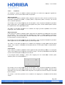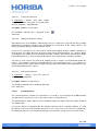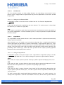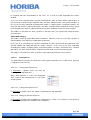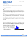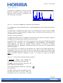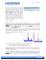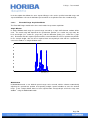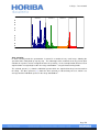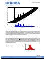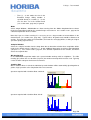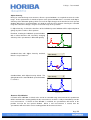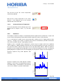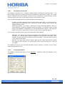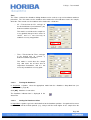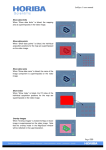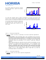
1
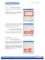
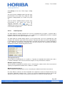
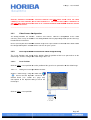
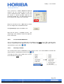
LabSpec 5 user manual
1.2
Intensity (cnt)
The spectrum shown to the right was acquired
without the “Spike Filter”. Spikes in the spectrum
are highlighted.
1.0
0.8
0.6
500
1 000
1 500
Raman Shift (cm-1 )
2 000
The “Spike Filter” algorithm compares multiple accumulations of a spectrum and calculates what
peaks are real (e.g., Raman peaks) and what peaks are spikes. It then automatically removes spikes
from the spectrum. The comparison method ensures that real peaks can never be incorrectly deleted.
1.2
Intensity (cnt)
The spectrum shown to the right was acquired with
the “Spike Filter” active. This time all peaks in the
spectrum are Raman peaks, and there are no
spikes visible.
1.0
0.8
0.6
500
3.5.4.7.1.
1 000
1 500
Raman Shift (cm-1 )
2 000
Turning On the “Spike Filter”
In Acquisition > Options select either “On (auto add)” or “On” from the “Spike Filter” drop down box.
o
o
3.5.4.7.2.
On (auto add): this mode automatically adds an extra accumulation to your measurement.
For example, if you specify three accumulations in the control panel (see section 9.9.3, page
235) the actual number acquired will be four (3+1). This mode ensures that every spectrum
will be spike filtered, even if you only specify one accumulation (since the software will
automatically acquire two accumulations (1+1) to enable the “Spike Filter” comparison
algorithm).
On: this mode will activate the “Spike Filter” only if the number of accumulations set in the
control panel (see section 9.9.3, page 235) is greater than 1. So, if an acquisition is made
with 2,3,4... accumulations, then the “Spike Filter” will be active. If an acquisition is made
with only 1 accumulation, then the “Spike Filter” will be inactive, and there is the possibility
of spikes being present in your spectrum. This mode is useful since it allows you to easily
switch between a fast analysis mode without the “Spike Filter” (e.g., when the accumulation
number is set to 1), and standard analysis with the “Spike Filter” (e.g., when the
accumulation number is set to 2 or more)
Turning Off the “Spike Filter”
In Acquisition > Options select “Off” from the “Spike Filter” drop down box.
Page | 38
LabSpec 5 user manual
3.5.4.8.
Autofocus
The “Autofocus” function sets how the autofocus operation (see section 3.5.8, page 59) is applied to a
measurement. There are three main modes of operation:
Before acquisition
In this mode, the autofocus procedure will be applied a single time at the start of a spectrum or array
acquisition (including time profiles, Z (depth) profiles, temperature profiles, XY maps, XZ and YZ
slices, and XYZ datacubes).
For example, if an XY map comprising 10 x 10 data points is to be acquired, the autofocus procedure
will be applied once at the beginning to find the optimal focus point, and the 100 data points will then
be acquired at the same optimal focus point.
This mode is useful when you wish to use autofocus for single spectrum acquisition, or for surface
mapping of a flat, smooth sample.
Before each point
In this mode, the autofocus procedure will be applied for each individual spectrum being measured in
the acquisition. For an array acquisition (including time profiles, Z (depth) profiles, temperature
profiles, XY maps, XZ and YZ slices, and XYZ datacubes) this means that the autofocus will be
performed before each point in the array.
For example, if an XY map comprising 10 x 10 data points is to be acquired, the autofocus procedure
will be applied at each XY coordinate prior to spectrum acquisition.
This mode is useful when you wish to use autofocus for mapping
mapping of a rough and/or non-flat (tilted)
sample. If the sample is smooth but non-flat (tilted) then the “In limits point” mode is recommended –
see below.
In limits point
In this mode, the autofocus procedure will be applied at four intermediate positions in a rectangular
surface (XY) mapping area to calculate
calculate the tilt of the sample. The focus position will then be adjusted
at each measurement point to compensate for the tilt.
In the diagram below showing a surface (XY) mapping area the intermediate “In-limits point”
autofocus points are marked with with “+”.
For example, if an XY map comprising 10 x 10 data points is to be acquired, the autofocus procedure
will be applied at the intermediate positions of the map area prior to the mapping. When the map
acquisition starts, the focus position will be adjusted
adjusted at each point, based on the tilt plane calculated
by the autofocus.
This mode is useful when you wish to use autofocus for mapping of a smooth but non-flat (tilted)
sample.
Page | 39
LabSpec 5 user manual
3.5.4.8.1.
Turning On Autofocus
In Acquisition > Options select either “Before
acquisition”, “Before each point” or “In limits point”
from the “Autofocus” drop down box.
Click [OK]. Autofocus is now active.
The Autofocus indicator icon is displayed in the
Status Bar.
3.5.4.8.2.
Setting the Autofocus Offset
Depending on the exact Autofocus mode being used (see section 3.5.8, page 59) the focus position
located by the autofocus procedure may correspond to a visual focus of the sample, which is not
always the position giving a maximum Raman signal.
In this case, it is possible to set a Z-axis offset, which will be applied after the autofocus position has
been located. A negative offset means that the focus will be moved upwards (e.g., analysis will be
made higher in the sample than the autofocus position); a positive offset means that the focus will be
moved downwards (e.g., analysis will be made lower in the sample than the autofocus position).
The offset is also useful if you wish to do mapping inside a sample at a fixed position below the
surface. The autofocus procedure (depending on the exact mode being used – see section 3.5.8,
page 59) will locate the surface of the sample, and the positive offset will then be applied to move to a
specified position below the surface.
3.5.4.8.3.
Turning Off Autofocus
In Acquisition > Options select “Off” from the
“Autofocus” drop down box.
Click [OK]. Autofocus is now inactive.
The Autofocus indicator icon is no longer displayed
in the Status Bar.
3.5.4.9.
Scanning Device
The “Scanning Device” function sets what device is used for Y axis movement in multidimensional
spectral array measurements (such as XY surface maps, or YZ depth slices).
The default mode is “Stage” which uses the motorized sample XY stage to move the sample in both X
and Y dimensions.
On systems which are equipped with the confocal LineScan mirror scanning hardware it is also
possible to use the LineScan to acquire data in the Y axis. In this case select “Scanner” to disable the
XY motorized stage for Y axis movement during the measurement, and to use the LineScan mirror.
Page | 40
LabSpec 5 user manual
3.5.4.10.
Use Detector
The “Use detector” function sets how multiple detectors are used during a measurement. If your
Raman system is equipped with a single detector only, then this option will be set to “Active” and will
be greyed out.
3.5.4.10.1. Setting the Use Detector Mode
In Acquisition > Options select either “Active” or “Both” from the “Use Detector” drop down box.
Active
In this mode data will only be acquired from the active detector. The active detector is selected from
the status bar (see section 7.3.2, page 201).
Both
In this mode it is possible to acquire data from two detectors simultaneously, but this only applies to
very specific configurations. For most standard systems, it is only ever possible to acquire data from
the active detector.
3.5.4.11.
Signal Mode
The “Signal Mode” function controls whether a ‘dark’ subtract procedure is implemented automatically
during a spectrum acquisition.
Some detectors (e.g., the InGaAs near infra-red array detector) have a significant fixed pattern
artefact signal which can dominate the spectrum acquired from a sample with low signal level. In this
case, it is possible to acquire a ‘dark’ spectrum (e.g., a spectrum acquired with a shutter in front of the
detector, so that no sample signal is observed) which corresponds to the fixed pattern signal only. By
performing a ‘dark’ subtract (e.g., subtract the ‘dark’ spectrum from the sample spectrum) significant
improvement in spectrum quality can be realised.
3.5.4.11.1. Setting the Signal Mode
In Acquisition > Options select either “Signal”, “Dark”, “Signal-Dark” or “Signal-Dark (always)” from the
“Signal Mode” drop down box. These choices what type of spectrum is acquired from the detector.
Signal
In this mode, the sample spectrum (detector shutter open) will be acquired and displayed on screen.
Dark
In this mode, the ‘dark’ spectrum (detector shutter closed) will be acquired and displayed on screen.
Note that in this mode you will not see a spectrum corresponding to your sample.
Signal-Dark
In this mode, the ‘dark’ spectrum (detector shutter closed) will be automatically subtracted from the
sample spectrum (detector shutter open). The ‘dark’ spectrum will be acquired first, followed by the
sample spectrum.
The ‘dark’ spectrum will be acquired with identical acquisition settings as the sample spectrum – for
example, if the acquisition is set for two accumulations of 30s each, then the ‘dark’ spectrum will also
Page | 41
LabSpec 5 user manual
be acquired with two accumulations of 30s each.
doubled.
As a result, the total acquisition time will be
In the case of an extended range spectrum acquisition the ‘dark’ spectrum will be acquired once at
the start of the extended range acquisition only, and then subtracted from each spectral window. In
the case of an array acquisition (including time profiles, Z (depth) profiles, temperature profiles, XY
maps, XZ and YZ slices, and XYZ datacubes), the ‘dark’ spectrum will be acquired once at the start of
the acquisition only, and then subtracted from the spectrum acquired at each measurement point.
This mode is useful when the ‘dark’ spectrum is constant, and is not expected to change between
measurements.
Signal-Dark (always)
This mode is similar to “Signal-Dark” discussed above. However, in this case, the ‘dark’ spectrum is
acquired before each and every readout from the detector.
In the case of an extended range spectrum acquisition the ‘dark’ spectrum will be acquired for each
spectral window and subtracted from the sample spectrum. In the case of an array acquisition
(including time profiles, Z (depth) profiles, temperature profiles, XY maps, XZ and YZ slices, and XYZ
datacubes), the ‘dark’ spectrum will be acquired and subtracted at each measurement point.
This mode is useful when the ‘dark’ spectrum is expected to vary between measurements.
3.5.4.12.
Autoexposure
The Auto Exposure function sets whether the auto exposure operation (see section 3.5.10, page 65)
is applied to a measurement.
3.5.4.12.1. Turning Auto Exposure On
In Acquisition > Options select “On” from the
“Autoexposure” drop down box.
When Auto Exposure is active, the Acquisition
Time section in the Control Panel is set to “Auto”
and greyed out.
3.5.4.12.2. Turning Auto Exposure Off
In Acquisition > Options select “Off” from the “Autoexposure” drop down box.
3.5.4.12.3. Setting Up the Auto Exposure
In Acquisition > Options click on [Set] in the “Autoexposure” section. See section 3.5.10, page 65, to
learn how the Auto Exposure function can be configured.
Page | 42
LabSpec 5 user manual
3.5.4.13.
Shutter Mode
The “Shutter Mode” function sets the operation of the detector shutter during an acquisition.
3.5.4.13.1. Setting the Shutter Mode
In Acquisition > Options select “Auto”, “Open” or “Closed” from the “Shutter Mode” drop down box.
Auto
In this mode, the shutter operation is set automatically by LabSpec 5. Typically this means that for
standard spectrum and array acquisition the shutter will be opened during spectrum acquisition, and
closed during detector readout and other system processes (such as moving the sample stage, or
spectrometer grating). For ultra-fast SWIFT™ mapping (see 4.5.5, page 97) the shutter is opened at
the start of the acquisition, and then kept open throughout the acquisition. It is closed only once the
final spectrum has been acquired.
Open
In this mode, the shutter will be kept open throughout an acquisition. For example, for an extended
range spectrum acquisition (see section 3.5.6, page 49) the shutter will be opened prior to acquisition
of the first spectral window, and will be kept open throughout the acquisition. It is closed only once
the final spectral window has been acquired.
Closed
In this mode, the shutter will be kept closed throughout an acquisition – it can be used to monitor the
inherent background ‘dark’ response of the detector. This mode can be used to assess the spectrum
of a detector without any light. Note that in this mode you will not see a spectrum corresponding to
your sample.
3.5.4.14.
Intensity Correction
The LabSpec 5 intensity correction algorithm allows true comparison of spectra acquired using
different laser wavelengths and optics. Without intensity correction, spectra acquired using different
laser wavelengths and optics can show significant differences in relative peak intensities. These
differences are caused by varying performance of the instrument components (including microscope
objectives, laser rejection filters, diffraction gratings and CCD detectors) at different wavelengths.
The spectrum shown right for 4-acetyl salicylic acid
was acquired using a 785 nm near infra-red laser.
In this case the CCD detector sensitivity decreases
as the Raman shift increases.
Thus peak
intensities at high Raman shift positions are
observed to be significantly weaker than they really
are. The observed spectrum is not correct, since it
is perturbed by instrumental factors.
500
1 000
1 500
2 000
-1
Raman Shift (cm )
2 500
3 000
3 500
Page | 43
LabSpec 5 user manual
By applying the “HORIBA ICS” intensity correction
factor the perturbed Raman spectrum peak
intensities can be restored, as illustrated in the
corrected spectra shown right.
500
1 000
1 500
2 000
Raman Shift (cm-1 )
2 500
3 000
3 500
3.5.4.14.1. How is the “HORIBA ICS” Correction Factor Calculated?
The “HORIBA ICS” intensity correction factor is created individually for each instrument at the time of
manufacture.
The output from a calibrated white light source is passed through the system, and the recorded
“response” spectrum is compared with the calibrated “source” spectrum of the white light source. The
correction factor is calculated as
correction = [source] / [response]
The obtained correction factor is a multiplicative factor, which means that each spectrum acquired is
multiplied by the correction factor to yield the corrected spectrum.
A correction factor is created for each and every pairing of laser wavelength and diffraction grating
available on the instrument (e.g., 532nm-600gr/mm; 532nm-1800gr/mm; 633nm-600gr/mm;
633nm-1800gr/mm etc). When the automatic intensity correction is activated, the software
automatically applies the appropriate correction factor based on the active laser wavelength and
diffraction grating pair.
In the event that there are multiple laser rejection filters for a single laser wavelength configured on a
LabRAM HR system (e.g., one notch filter and one edge filter for 633nm) the software cannot
automatically detect which filter is in place. In this case, the specific laser filter must be selected from
Setup > ICS Filters before the acquisition is made – see section 3.7.3, page 75, for further
information.
3.5.4.14.2. Turning On the Automatic Intensity Correction
In Acquisition > Options, select “HORIBA ICS”
from the “Intensity Correction” drop down box.
Click [OK]. Intensity Correction is now active, and
will be applied to all acquired data.
The Intensity Correction indicator icon is displayed
in the Status Bar.
If multiple injection/rejection or photoluminescence
(PL) filters have been set up for a single laser
wavelength ensure the correct filter is selected
Page | 44
LabSpec 5 user manual
from the ICS Filters dialog window, by clicking on
Setup > ICS Filters.
Note that an intensity correction factor must have
been created for the specified laser wavelength
and diffraction grating pair, otherwise an error
message similar to that shown right will be
displayed when an acquisition is started. Click on
[OK] or [Cancel] to clear the message, and start
the acquisition. Remember that in this case the
spectrum will be uncorrected. The error message
will only be shown once during a LabSpec session
– if LabSpec is closed and then re-opened, the
message will be displayed again if intensity
correction is activated when no intensity correction
factor has been created.
3.5.4.14.3. Turning Off the Automatic Intensity Correction
In Acquisition > Options, select “Off” from the
“Intensity Correction” drop down box.
Click [OK]. Intensity Correction is now inactive.
The Intensity Correction indicator icon is no longer
displayed in the Status Bar.
3.5.4.14.4. Applying Post-acquisition Intensity Correction
Ensure that the correct laser wavelength and
diffraction grating pair are selected in the Control
Panel.
If multiple injection/rejection or photoluminescence
(PL) filters have been set up for a single laser
wavelength ensure the correct filter is selected
from the ICS Filters dialog window, by clicking on
Setup > ICS Filters.
Select the spectrum which is to have the Intensity
Correction applied post-acquisition.
In Acquisition > Options, select “HORIBA ICS”
from the “Intensity Correction” drop down box.
Click on [Correct] in the Intensity Correction
section.
Click [OK]. The Intensity Correction has now been
applied to the spectrum.
Page | 45
LabSpec 5 user manual
Note that an intensity correction factor must have
been created for the specified laser wavelength
and diffraction grating pair, otherwise an error
message similar to that shown right will be
displayed when an acquisition is started. Click on
[OK] or [Cancel] to clear the message.
Remember that in this case the spectrum will
remain uncorrected. The error message will only
be shown once during a LabSpec session – if
LabSpec is closed and then re-opened, the
message will be displayed again if intensity
correction is activated when no intensity correction
factor has been created.
3.5.4.15.
Denoise
The Denoise function is a unique noise reduction algorithm which can be used to significantly
enhance spectrum quality without losing subtle spectral information. When Denoise is activated in
Acquisition > Options, all data acquired will be processed with the Denoise reduction – this includes
real time display (RTD) acquisition (
spectral array acquisition (
/
/
), spectrum acquisition (
/
) and multidimensional
).
Standard smoothing functions can result in loss of peak shape and position, and subtle features (such
as weak shoulders on a strong band) can be lost. The Denoise function ensures that all this important
information is retained, whilst still reducing noise in the spectrum.
The spectra shown right illustrate the effect of the
Denoise function.
Two main Denoise algorithms are available from the “Denoise” drop down box:
o
o
Standard: recommended for spectra with signal to noise ≥ 20
Lite: recommended for very noisy spectra with signal to noise ≤ 20
In addition, both algorithms can be used with an integrated Despike function to remove random spikes
(also known as cosmic rays). See also section 3.5.4.7, page 37, for more information about other
spike filter options in LabSpec 5.
Denoise can be applied post-acquisition using the Smoothing icon and Filtration dialog window – see
section 4.6.4, page 124. If a spectrum has had the Denoise function automatically applied through
Acquisition > Options, it cannot have the function applied again through the Filtration dialog window.
Page | 46
LabSpec 5 user manual
3.5.4.15.1. Turning On the Automatic Denoise Function
In Acquisition > Options select the desired Denoise function from the “Denoise” drop down box:
o
o
o
o
Standard: recommended for spectra with signal to noise ≥ 20
Standard + Despike: as “Standard” but with an integrated Despike function to remove
random spikes (also known as cosmic rays)
Lite: recommended for very noisy spectra with signal to noise ≤ 20
Lite + Despike: as “Lite” but with an integrated Despike function to remove random spikes
(also known as cosmic rays)
Note that this function will be automatically applied to all data acquisition.
3.5.4.15.2. Turning Off the Automatic Denoise Function
In Acquisition > Options select “Off” from the “Denoise” drop down box.
3.5.5.
Auto save
The autosave function allows data to be saved automatically when a measurement is completed.
This function is useful to ensure that important data is immediately saved, so that there is no risk of
loss of data caused by intervention of another user, power cut, or computer crash.
Note that the autosave function can only be activated for spectrum acquisition (
/
) and
multidimensional spectral array acquisition (
/
). Real time display (RTD) data (see section
4.5.1, page 95) will not be autosaved, even if the autosave function is activated in LabSpec 5.
3.5.5.1.
Setting the Autosave Function
The Autosave function can be configured to automatically save data in a specific format to a specific
location.
Save acquired data
If the “Save acquired data” box is ticked the Autosave function is active, and data will be automatically
saved.
Page | 47
LabSpec 5 user manual
Auto repeat
If the “Auto repeat” box is ticked a spectrum acquisition (
the STOP icon (
next spectrum.
/
/
) will be continuously repeated until
) is clicked. Each spectrum displayed on the screen will be replaced by the
If the “Save acquired data” box is also ticked each individual spectrum will be automatically saved.
Format
Select the file format from the drop down box which will be used to save the data. Please see section
3.1.1.1, page 10, for full details about available file formats.
o
o
o
o
LabSpec (*.ngs) – data will be saved in its inherent LabSpec 5 format. Spectra will be
saved as .ngs, and multidimensional spectral arrays (including time profiles, Z (depth)
profiles, temperature profiles, XY maps, XZ and YZ slices, and XYZ datacubes) will be
saved as .ngc.
Dilor (*.ms0) – data will be saved a legacy file format for Dilor Raman instruments.
Grams (*.spc) – data will be saved in a Grams SpectraCalc spectrum file format, compatible
with many common spectroscopy software packages.
LabSpec (*.tsf) – data will be saved in the previous generation LabSpec 4 format. Spectra
will be saved as .tsf, and multidimensional spectral arrays (including time profiles, Z (depth)
profiles, temperature profiles, XY maps, XZ and YZ slices, and XYZ datacubes) will be
saved as .tvf.
Folder
Type in the file path (or browse using the file browse button) for the location where the data should be
saved.
o
o
If the folder exists already, data will be saved inside the specified folder. Tick the boxes for
“Year”, “Month” and “Day” to create a new folder labelled “_YYYY_MM_DD”, which indicates
the year (YYYY), month (MM) and day (DD) according to the computer’s clock.
If the folder does not already exist it will be created when the Autosave procedure is next
performed. If the boxes for “Year”, “Month” and “Day” are ticked, the year (YYYY), month
(MM) and day (DD) according to the computer’s clock will be appended to the specified
folder name (for example, “Folder_YYYY_MM_DD”).
File
Type in the file name for the data which is to be saved. Tick the “Hour”, “Min” and/or “Count” boxes to
append the hour (HH), minute (mm) and/or integer count (C) to the file name. The count number will
start at the number indicated in the box – to start the count at a different number type in the desired
first number in the count box. This number will be automatically incremented for subsequent
autosaves.
For example, with “Hour” and “Min” ticked, the data will be saved as “FileName_HH_mm.xxx” where
“.xxx” indicates the specified file format.
With “Count” ticked, the data will be saved as “FileName_C.xxx” where “.xxx” indicates the specified
file format.
Page | 48
LabSpec 5 user manual
3.5.5.2.
Turning On the Autosave Function
In Acquisition > Autosave, tick the box for “Save
acquired data”.
3.5.5.3.
Turning Off the Autosave Function
In Acquisition > Autosave, untick the box for “Save
acquired data”.
3.5.6.
Extended Range
The Extended Range dialog window controls the spectral range which will be analysed during a
/
) or multidimensional spectral array acquisition (
/
). When an
spectrum acquisition (
extended range is specified, the software will acquire multiple spectra and seamlessly glue them to
give a final spectrum corresponding to the desired extended range.
Page | 49
LabSpec 5 user manual
In the description that follows the term “Spectral Range” refers to the specified extended range, and
“Spectral Window” refers to the individual spectra which are acquired to cover the extended range.
3.5.6.1.
Extended Range Acquisition Modes
The Extended Range module offers three main modes for spectrum acquisition.
Single Window
In Single Window mode, only the spectral range covered by a single CCD detector readout will be
used. The actual range will depend on the spectrometer position (see section 9.5, page 230), the
laser wavelength (see section 9.1, page 227), and the diffraction grating (see section 9.6.1, page
231). Remember that the acquired spectrum will be centered about the current spectrometer position.
In the example below, data has been acquired from 4-acetylsalicylic acid with the spectrometer
-1
centered at 1200cm in Single Window mode.
-1 000
0
1 000
Raman Shift (cm-1 )
2 000
3 000
4 000
Multiwindow
In Multiwindow mode, a user defined spectral range can be covered, with the software automatically
adjusting the spectrometer position and capturing multiple spectral windows to cover the desired
range. In the example below, data has been acquired from 4-acetylsalicylic acid in the range 100-1
3500cm using the Multiwindow mode.
Page | 50
LabSpec 5 user manual
Spectral
Window 1
-1 000
0
Spectral
Window 2
1 000
Raman Shift (cm-1 )
Spectral
Window 3
2 000
Spectral
Window 4
3 000
4 000
Auto scanning
In Auto scanning mode the spectrometer is moved in a number of very small steps, allowing the
spectrum to be slowly built up step by step. The advantage of this method is that any pixel to pixel
variation in response can be averaged out over the spectrum. In the example below, data has been
-1
acquired from 4-acetylsalicylic acid in the range 100-3500cm using the Autoscanning mode.
The stacked spectra (—) show the individual spectra which are acquired, but they have been offset
for clarity. The blue spectrum (—) shows the final spectrum as observed by the user, which is an
-1
average of all the individual spectra, in the range 100-3500cm .
Page | 51
LabSpec 5 user manual
-1 000
3.5.6.2.
0
1 000
Raman Shift (cm-1 )
2 000
3 000
4 000
Sub-pixel Acquisition Function
The Sub-pixel acquisition function uses the high precision, fine step size of the spectrometer drive
mechanism to acquire spectra which are shifted by less than a whole pixel value. The result is to
increase the number of data points defining a band (i.e., sub-pixel = 2 results in twice the number of
data points; sub-pixel = 3 results in three times the number etc).
Note that this will increase the total acquisition time, and it is suggested that sub-pixel acquisition is
only used over limited ranges.
The sub-pixel acquisition function does not increase the spectral resolution of the spectrometer, since
this is defined principally by the laser wavelength, spectrometer focal length, diffraction grating and
slit. However, the sub-pixel acquisition function is useful to give increased definition of a peak, by
providing more data points to define that peak. This can be beneficial when studying peak shape, or
performing peak fitting routines.
6000
5000
Intensity (a.u.)
Sub-pixel = 1
The data shown right has been acquired with
sub-pixel = 1, which is the default value for
standard acquisitions.
4000
3000
2000
1000
0
510
515
520
525
Wavenumber (cm-1)
Page | 52
LabSpec 5 user manual
6000
5000
Intensity (a.u.)
Sub-pixel = 4
The data shown right has been acquired with
sub-pixel = 4. The increased number of data
points is clearly visible.
4000
3000
2000
1000
0
510
515
520
525
Wavenumber (cm-1)
3.5.6.3.
Setting the Extended Range
From and To
Set the beginning (“From”) and end (“To”) spectral
positions by typing in the desired values into the
respective boxes. The spectral units are those
which are displayed in the spectrometer window in
the control panel (see section 9.5, page 230),
and/or selected via Options > Unit (see section
3.4.1, page 22).
Note that multiple spectral windows can be set up
by ticking the check boxes on the right hand side.
Up to five spectral ranges can be defined. Each
spectral range can be acquired with a specific
integration time – see Time below.
Multiple spectral ranges can be contiguous (e.g.,
-1
100-200, 200-500, 500-2000cm ) or discrete (e.g.,
-1
100-1500, 1750-1900, 2900-4000cm ).
For most standard measurements it is generally
sufficient to use a single spectral range covering
the whole range desired.
Time
The acquisition time for each spectral range can be
set up in two ways.
o
Time (%) – in this mode, the time in the
Extended Range dialog window is
specified as a percentage (%) of the
acquisition time set in the Control Panel
(see section 9.9.2, page 235).
For
example, if the Control Panel has the
acquisition time set as 10s, then if Time
(%) is set to 50% in the Extended Range
dialog window, the acquisition will be
made with 5s per spectral window.
Page | 53
LabSpec 5 user manual
o
Time (s) – in this mode, the time in the
Extended Range dialog window is
specified directly in seconds (s). In this
case the time set in the Control Panel
(see section 9.9.2, page 235) is ignored.
Mode
Select “Single Window”, “Multiwindow” or “Auto scanning” from the “Mode” drop down box to choose
the desired acquisition mode for the extended range measurement. See section 3.5.6.1, page 50, for
a detailed explanation of these modes.
Note that if you use “Auto scanning” it is necessary to set a larger number of accumulations in the
Control Panel (see section 9.9.3, page 235). Typical values for good results would be between 10
and 50. The larger the number of accumulations, the better the averaging will be, resulting in a higher
spectrum quality (signal to noise).
Sub-pixel Number
Select the sub-pixel number from the drop down box to determine whether data acquisition will be
made in the default manner (sub-pixel = 1), or with additional data points to enhance band definition
(sub-pixel > 1). See section 3.5.6.2, page 52, for a detailed explanation of this function, and how it
affects the acquired data.
Min Overlap (pix)
In the Multiwindow acquisition mode each spectral window overlaps with its neighbours. The “Min
Overlap (pix)” allows the user to define (in pixels) the minimum overlap which must be used. Typically
a value of 100 is adequate for most measurements.
Combine Data
When “Combine Data” is ticked, the individual spectral windows will be automatically glued together to
yield a single spectrum at the completion of the measurement.
Spectrum acquired with “Combine Data” unticked:
1 000
2 000
Raman Shift (cm-1 )
3 000
1 000
2 000
Raman Shift (cm-1 )
3 000
Spectrum acquired with “Combine Data” ticked:
Page | 54
LabSpec 5 user manual
Adjust Intensity
During an extended range measurement, discrete spectral windows are acquired to cover the entire
range. As the spectrometer is moved to capture each spectral window there is a natural small drop in
efficiency of the diffraction grating, which can result in slight changes to the baseline of each spectral
window. When these spectral windows are glued to create the final spectrum covering the extended
range these baseline changes can give rise to small steps in the spectrum.
If “Adjust Intensity” is ticked, the baselines of the individual spectral windows will be adjusted prior to
gluing, to yield a seamless final spectrum.
Raw data, showing the individual spectral windows
with a natural baseline shift caused by changing
efficiency of the spectrometer’s diffraction grating.
2 900
3 000
3 100
Raman Shift (cm-1 )
3 200
2 900
3 000
3 100
Raman Shift (cm-1 )
3 200
2 900
3 000
3 100
Raman Shift (cm-1 )
3 200
Combined data, with “Adjust Intensity” unticked.
-1
Note the step at 3030 cm .
Combined data, with “Adjust Intensity” ticked. The
gluing between the two individual spectral windows
is seamless.
Return to First Window
If “Return to First Window” is ticked, at the end of an extended range measurement the spectrometer
will be returned to the starting position for the measurement, so that it is ready to immediately start the
next measurement. If “Return to First Window” is unticked, the spectrometer will remain at the
position used for the last spectral window. When a new measurement is started, then the
spectrometer will move to the correct starting position for that measurement.
Page | 55
LabSpec 5 user manual
The “Return to First Window” function is particularly
particularly useful when making kinetic time based
measurements with the extended range function. In this case it is important that the spectrometer is
ready to immediately start the measurement at the next trigger point for the kinetic run, and thus, it
must be at the starting position for the extended range in advance.
3.5.6.4.
Turning On the Extended Range Function
In the extended range dialog window (accessed
via Acquisition > Extended range, or the Extended
range icon
/
) select the desired extended
range mode from the “Mode” drop down box.
Choose either “Multi windows” or “Auto scanning”
to make an extended range measurement.
Set up the spectral range and other options
(section 3.5.6.3, page 53), and click [OK]. The
extended range function is now active.
The extended range indicator icon is displayed in
the Status Bar.
Note that the extended range is only available for
full
spectrum
acquisition
(
/
),
or
multidimensional spectral array acquisition (
/
). It is not available for real time display
(RTD) (
3.5.6.5.
/
).
Turning Off the Extended Range Function
In the extended range dialog window (accessed
via Acquisition > Extended range, or the Extended
range icon
/
) select the “Single window”
mode from the “Mode” drop down box.
Page | 56
LabSpec 5 user manual
All the options will be greyed out.
Click [OK]. The extended range function is now
inactive.
The extended range indicator icon is no longer
show in the Status Bar.
3.5.7.
Detector
The detector window controls the configuration of the detector(s) used by the Raman system. In
typical use these parameters do not need to be adjusted by the user, and it is recommended that they
are only modified when instructed to do so by a trained engineer from HORIBA Scientific or one of its
representatives.
Page | 57
LabSpec 5 user manual
_________________________________________________________________________________
CAUTION: CHANGING SETTINGS IN THE ACQUISITION > DETECTOR WINDOW MAY RESULT IN SYSTEM
MALFUNCTION. ON NO ACCOUNT SHOULD SETTINGS IN THIS DIALOG WINDOW BE MODIFIED EXCEPT WHEN
INSTRUCTED TO DO SO BY A TRAINED ENGINEER FROM HORIBA SCIENTIFIC OR ONE OF ITS
REPRESENTATIVES.
_________________________________________________________________________________
Type
Select the detector to be used from the “Sensor” drop down box – this list will only show the detectors
installed on the instrument.
Note that when multiple detectors are installed the
active detector can also be selected using the
detector indicator in the Status Bar (see section
7.3.2, page 201).
Select the read out mode for the detector from the “Mode” drop down box. For two dimensional array
detectors (such as a CCD), the software has different read out zones (areas) configured, one for
spectrum acquisition, and one for area intensity acquisition.
o
o
Spectrum – select this mode for acquiring normal spectra where the detector is used in a
one dimensional configuration (spectral axis).
Image – select this mode for specialized applications where the detector is used in a two
dimensional configuration (spectral axis and CCD height).
Sizes
The “Sizes” section controls what area of the detector is used for the “Spectrum” and “Image” modes.
Type in the desired minimum and maximum pixel numbers
numbers to define the area which will be used. The
values in the greyed out boxes indicate the maximum pixel size of the detector in the X and Y axes.
Options
The options visible will depend on the particular detector(s) installed on the instrument. Please
consult a trained engineer from HORIBA Scientific or one of its representatives to find out more about
the options available for the detectors installed on your system.
In most cases, the temperature sensor and control options will be present, and these are described
below.
3.5.7.1.
Displaying the Detector Temperature
Click on the “temperature” icon to display the
current temperature of the detector.
o
The current temperature (in degrees celsius, C)
will be displayed in the adjacent indicator box.
-70
Page | 58
LabSpec 5 user manual
Tick the box to have the current temperature
continuously updated.
-70
Note that the current temperature of the active
detector is also displayed next to the detector
indicator icon in the Status Bar.
3.5.7.2.
-70
Setting the Detector Temperature
To set the temperature of the detector, type in the
o
desired value (in degrees celsius, C), and click
[Set].
3.5.8.
Autofocus
The Autofocus function in LabSpec 5 automatically finds the optimum focus position for a sample, and
ensures that the best quality spectrum with maximum signal level can be easily achieved.
It is a useful tool for samples where manual focusing is difficult (such as highly polished, clean
surfaces). So long as the sample is relatively close to focus the Autofocus procedure will find the
correct focus position and give a good quality spectrum.
Autofocus also is invaluable when acquiring XY surface maps of samples which have significant
surface roughness. Without autofocus whenever the measurement position in the map is out of focus
the signal level will be reduced, and analysis of the map data will be difficult. With the autofocus
running, the focus position will be adjusted at each measurement position in the map, ensuring that
good quality data is acquired across the full mapping area, despite the sample’s inherent roughness.
6 000
Intensity (cnt)
Spectrum acquired using 100x objective with
autofocus.
4 000
2 000
1 500
1 000
-1
Raman Shift (cm )
1 500
1 000
-1
Raman Shift (cm )
1 500
Intensity (cnt)
350
300
250
200
150
8 000
6 000
Intensity (cnt)
Spectrum acquired using 100x objective without
autofocus; out of focus by approximately 20 µm.
The bottom image is shown with the same intensity
scale as the ‘autofocus’ spectrum shown above.
1 000
-1
Raman Shift (cm )
4 000
2 000
0
Page | 59
LabSpec 5 user manual
3.5.8.1.
The Autofocus Procedure
The Autofocus procedure uses a software controlled motor to control the microscope focus. The
focus position is adjusted in small increments whilst monitoring a signal from the sample. The sample
signal is maximum at the focus position, and thus the focus adjustment is made iteratively until the
maximum signal is observed. At this point, the Raman measurement is made.
There are two main motors which are used to control the microscope focus.
o
o
Z motor – this motor controls the fine focus wheel of the microscope. Its maximum range is
limited only by the microscope focus mechanism, and the available space between the
objective and the sample.
Piezo device (Pifoc) – this motor is attached to a single microscope objective, and uses
piezo controllers to adjust the objective position up or down. Its maximum range is limited
by the piezo controllers, and typically has a travel of approximately 100 µm. By using piezo
motors, this device is extremely fast, and has very fine step size (typically <50 nm).
There are two main signals which can be detected to find the focus position.
o
o
Reflection – this signal is the reflected and Rayleigh scattered light from the sample, and is
detected by a small pin diode detector positioned at the top of the microscope, which
monitors the total signal intensity (without spectral information). The signal will be greatest
at the surface of the sample.
Detector – this signal is based on the Raman signal from the sample detected in the normal
way using the active detector. The signal will be greatest at (or just below) the surface of
the sample.
The hardware present on your instrument will dictate whether autofocus is possible, and if so, what
motor and signal will be used.
3.5.8.2.
Setting Up Autofocus
The Autofocus dialog window (accessed via Acquisition > Autofocus) allows the Autofocus to be
configured.
Page | 60
LabSpec 5 user manual
Z parameters
Select the motor type from the “Device” drop down box. Depending on the instrumentation
configuration there may only be one motor available. The typical devices which are used are as
follows:
o
o
Motorized – this uses the Z motor connected to the fine focus wheel of the microscope.
Pifoc – this uses the piezo Z axis motor attached to a specific objective.
Select the scan type from the adjacent drop down box. There are two types of autofocus scans which
can be used:
o
o
Continuous – the motor will make a continuous sweep through the Z axis, whilst reading out
the signal.
Step by step – the motor will move to a set position, then read out the signal; then move to
the next position etc.
Set the Z scan “Range” and “Step”. The range must be set sufficiently large to ensure that the
sample’s roughness can be countered using Autofocus; however the range must not be set so large
that the objective would be driven into the sample. With the “Motorized” Z motor device the range is
only limited by the microscope focus mechanism, and the available space between the objective and
the sample. With the “Pifoc” piezo motor the range is limited by the piezo controllers, and typically
has a travel of approximately 100 µm.
_________________________________________________________________________________
CAUTION: TAKE CARE SETTING THE Z SCAN “RANGE” WHEN USING THE Z MOTOR (“MOTORIZED” DEVICE). IF
THE RANGE IS SET LARGER THAN THE AVAILABLE SPACE BETWEEN THE SAMPLE AND THE OBJECTIVE, THE
SAMPLE, OBJECTIVE, MICROSCOPE AND/OR Z MOTOR COULD BE SERIOUSLY DAMAGED.
_________________________________________________________________________________
Signal
Select the autofocus signal from the “Signal” drop down box.
o
o
Reflection - this signal is the reflected and Rayleigh scattered light from the sample, and is
detected by a small pin diode detector positioned at the top of the microscope, which
monitors the total signal intensity (without spectral information).
Detector - this signal is based on the Raman signal from sample detected in the normal way
using the active detector.
Tick the “Profile” box to create a profile of signal intensity versus Z (depth) position during the
autofocus procedure. This can be a useful tool to monitor and troubleshoot the autofocus procedure.
If “Reflection” signal is selected, there are no other parameters which need to be set in the “Signal”
section.
If “Detector” signal is selected, specify the spectral range which will be used to optimise the focus
position, and set the “exposure” (acquisition) time (in seconds, s) which will be used for the autofocus
spectrum read out. Note that this exposure time is used only for the autofocus procedure – once the
focus position is located the sample measurement will be made using the acquisition parameters set
in the Control Panel (see section 9.9, page 234).
Page | 61
LabSpec 5 user manual
Zone
The “Zone” section of the Autofocus dialog window can be used to set up an intermittent autofocus
procedure. The “XY” mode sets the autofocus to be made after a fixed distance across the sample,
whilst the “Time” mode sets the autofocus to be made after a fixed time.
o
XY – Tick the box for “XY”, and type in
the desired distance (in micrometers, µm)
between autofocus operations.
This mode is useful when the sample has
a very gradual change in focus across its
surface, and it is not necessary to
autofocus at every map position.
o
Time – Tick the box for “Time”, and type
in the desired time (in seconds, s)
between autofocus operations.
This mode is useful when the sample
may slow move out of focus due to
temperature fluctuations, and it is not
necessary to autofocus at every point.
3.5.8.3.
Turning On Autofocus
In Acquisition > Options, select the appropriate mode from the “Autofocus” drop down box (see
section 3.5.4.8.1, page 40).
Click [OK]. Autofocus is now active.
The Autofocus indicator icon is displayed in the
Status Bar.
3.5.8.4.
Setting the Autofocus Offset
In Acquisition > Options, type in the desired offset for the Autofocus position. A negative offset means
that the focus will be moved upwards (e.g., analysis will be made higher in the sample than the
Page | 62
LabSpec 5 user manual
autofocus position); a positive offset means that the focus will be moved downwards (e.g., analysis
will be made lower in the sample than the autofocus position). See section 3.5.4.8.2, page 40, for
further information.
3.5.8.5.
Turning Off Autofocus
In Acquisition > Options select “Off” from the “Autofocus” drop down box (see section 3.5.4.8.3, page
40).
Click [OK]. Autofocus is now inactive.
The Autofocus indicator icon is no longer displayed in the Status Bar.
3.5.9.
Extra Images
The “Extra Images” dialog window allows extra images to be recorded using other detector devices on
the system (such as the Autofocus “reflection” pin diode detector – see section 3.5.8, page 59).
There are two main modes:
o
o
3.5.9.1.
Image – this allows for stand alone images to be recorded using the signal from the
additional detector. The dimensions of the image (in X, Y and/or Z axes) and the number of
image pixels are defined in the “Extra Images” dialog window.
Map – this allows signal from the additional detector to be recorded simultaneously with a
multidimensional spectral array measurement (such as a Raman XY surface map). The
dimensions of the image (in X, Y and/or Z axes) and the number of data points are taken
from the “Mapping Properties” dialog window (see section 4.5.5, page 97) and do not need
to be set in the “Extra Images” dialog window.
What are Extra Images For?
The “Extra Images” function can be useful to obtain additional information about a sample which
wouldn’t normally be possible on a Raman microscope.
One typical example is to create a map of the sample’s surface topography (roughness). This can be
done by using information obtained during the Autofocus procedure (see section 3.5.4.8, page 39). If
the Autofocus procedure is used for a Raman XY map of the surface at each measurement point in
the map the software has calculated a focus position based on an autofocus signal. These two values
(focus position and signal) directly reflect the topography of the sample. The “Extra Images” function
allows the topography image to be created simultaneously with the Raman map.
Page | 63
LabSpec 5 user manual
3.5.9.2.
Setting Up an Image Acquisition
Tick the axis boxes to activate the X, Y and Z axes
as required.
Set the image dimensions (in micrometers, µm)
using the “From” and “To” boxes, and number of
image pixels using the “Size” boxes.
Select the signal source (additional detector) which
will be used to create the image, by ticking the
“Image” box(es) in the “Sources” section..
The most common sources are as follows:
o
o
Reflection – autofocus pin diode detector.
Z – Z-axis position of the piezo/Z motor.
Other sources may be visible in this dialog window,
depending on the configuration of your system.
Click [Image] to start the acquisition.
3.5.9.3.
Setting Up a Map Acquisition
Select the signal source (additional detector) which
will be used to create the mapped image by ticking
the “Map” box(es) in the “Sources” section.
Nothing needs to be set or adjusted in the “Image”
section of the dialog window. Note that if all three
image axes (X, Y and Z) are unticked, then the
[Image] button will be greyed out. This button is
not used for map acquisition.
Page | 64
LabSpec 5 user manual
Click [Close] to close the “Extra Images” dialog
window.
Set up the Raman multidimensional spectral array
measurement in the normal way using the “Map
Properties” dialog window (see section 4.5.5, page
97)
Start the Raman multidimensional spectral array
measurement in the normal way using the
“Mapping Acquisition” icon (
/
).
An
additional map image (or images) will be displayed
as the Raman map proceeds.
3.5.10.
Auto Exposure
The Auto Exposure function calculates the necessary acquisition time to acquire a spectrum with a
maximum signal level specified by the user. It is useful to ensure a good quality spectrum is acquired
regardless of the inherent signal strength of the sample.
The Auto Exposure function initially acquires a test spectrum with a fast ‘test’ acquisition time, and
calculates the maximum signal level in the spectrum. Based on this data a new ‘final’ acquisition time
is calculated to yield a maximum signal equal to the specified ‘desired intensity’, and the acquisition is
made. ‘Minimum’ and ‘Maximum’ acquisition times are also set by the user, to prevent the software
attempting an infinitely short or long measurement.
Test exposure time (s)
Set the initial test acquisition time, in seconds (s). Typically an acquisition time between 0.3s and 1s
is suitable, although it can be increased if most samples are very weak Raman scatterers.
Minimum exposure time (s)
Set the minimum acquisition time which can be selected by the software for the final measurement.
Typically an acquisition time between 0.1s and 0.5s is suitable.
Maximum exposure time (s)
Set the maximum acquisition which can be selected by the software for the final measurement.
For weak Raman scatterers the final acquisition time required to reach the ‘Desired intensity’ may
exceed the ‘Maximum exposure time’. In this case the final acquisition time will be equal to the
‘Maximum exposure time’ and the achieved intensity may be less than the ‘Desired intensity’.
Page | 65
LabSpec 5 user manual
Desired intensity (cnt)
Set the desired maximum signal level (in counts, cnt) for the final spectrum, ensuring that it is below
the saturation point of the detector being used. Remember that the larger the desired intensity the
longer the measurement will take, but the better the spectrum quality.
For weak Raman scatterers the ‘Desired intensity’ may not be achieved because the final acquisition
time required to reach this intensity would need to exceed the ‘Maximum exposure time’. In this the
‘Maximum exposure time’ is used.
3.5.10.1.
Turning the Auto Exposure Function On and Off
The Auto Exposure function is turned on and off
using the “Autoexposure” drop down box in
Acquisition > Options – see section 3.5.4.12, page
42.
When Auto Exposure is active, the Acquisition
Time section in the Control Panel is set to “Auto”
and greyed out.
3.5.11.
Heat Detector
For peltier cooled (liquid nitrogen free) detectors, the “Heat Detector” function will switch off the peltier
cooling and allow the detector to warm up to room temperature.
Cooling can be restarted either by setting the temperature in Acquisition > Detector (see section
3.5.7.2, page 59), or by exiting and restarting LabSpec 5.
3.6.
Video
The Video menu allows configuration of the instrument’s video camera(s), set up of video image
scaling and the laser spot marker position, and (when multiple cameras are present) selection of the
active camera.
Video camera configuration
Laser spot marker position and video image scaling and
List of installed cameras
Page | 66
LabSpec 5 user manual
_________________________________________________________________________________
CAUTION: CHANGING PARAMETERS ACCESSED THROUGH THE VIDEO MENU COULD CAUSE THE VIDEO
CAMERA(S) TO CEASE WORKING, OR TO WORK INCORRECTLY. YOU SHOULD ONLY MODIFY PARAMETERS IN
THE VIDEO MENU WHEN INSTRUCTED TO DO SO BY A TRAINED ENGINEER FROM HORIBA SCIENTIFIC OR ONE
OF ITS REPRESENTATIVES.
_________________________________________________________________________________
3.6.1.
Video Camera Configuration
The dialog windows for “Source”, “Format” and “Offsets” allow the configuration of the video
camera(s) to be set up, or modified. The dialog windows will vary depending to the specific camera(s)
installed on the instrument.
Please consult your local HORIBA Scientific engineer or representative to find out more details about
the configuration options available for the cameras on your system.
3.6.2.
Laser Spot Marker Position and Video Image Scaling
The “Laser Position” and “Image Scale” options allow the position of the laser spot marker on the
video image, and the scaling of the video images to be set.
3.6.2.1.
Laser Position
Click on Video > Laser position to set the position of the green laser spot
spot marker on the video image.
3.6.2.1.1.
Setting the Laser Spot Marker Position
Acquire a video image, using the video icon (
/ ). Ensure that the objective selected in the
Control Panel (see section 9.7, page 233)
corresponds to the objective being used on the
microscope.
Click on Video > Laser position.
Page | 67
LabSpec 5 user manual
Drag the green laser spot marker to the desired
position on the video image, or type the desired
coordinates into the “Center X” and “Center Y”
boxes.
Click [OK].
repositioned.
The laser spot marker is now
Note that this process is objective specific – the
laser spot marker position should be set for each
objective on the microscope.
3.6.2.2.
Video Image Scale
Click on Video > Image scale to open the “Image scale” dialog window.
A resizeable scale box will additionally appear on the video image. The scale box can be resized to a
known size, and the known values used to scale the video image.
3.6.2.2.1.
Setting the Video Image Scale Using the “1” “2” Corner Positions
Acquire a video image, using the video icon (
/ ). Ensure that the objective selected in the
Control Panel (see section 9.7, page 233)
corresponds to the objective being used on the
microscope.
Click on Video > Image scale to open the “Image
scale” dialog window.
Page | 68
LabSpec 5 user manual
Ensure the “Size X” and “Size Y” boxes are ticked.
Drag the scale box to cover a large proportion of
the video image.
Move a small, easily recognisable feature of the
sample so that it is positioned exactly at the top,
left hand corner of the scale box. Dust particles on
the Silicon calibration sample are ideal for this, but
any sample with recognisable features can be
used.
Click [1]. The scale values in the “Size X” and
“Size Y” boxes are cleared.
Using the joystick move the XY stage so that the
feature is positioned exactly at the bottom, right
hand corner of the scale box.
Page | 69
LabSpec 5 user manual
Click [2]. The scale values in the “Size X” and
“Size Y” boxes are set according to the distance
moved by the XY stage.
Click [Scale XY] to register the video scale.
Note that this process is objective specific – the
video image scale should be set for each objective
on the microscope.
3.6.2.2.2.
Setting the Video Image Scale Manually
Acquire a video image, using the video icon (
/ ). Ensure that the objective selected in the
Control Panel (see section 9.7, page 233)
corresponds to the objective being used on the
microscope.
Click on Video > Image scale to open the “Image
scale” dialog window.
Ensure the “Size X” and “Size Y” boxes are ticked
as appropriate. With this procedure it is possible to
scale just one dimension (X or Y) if desired. The
dimension(s) to be scaled must be ticked.
Drag the scale box (in X and/or Y dimensions, as
appropriate) to match a feature of known size.
Typically this will be a graticule scale bar, but any
sample feature of precisely known size can be
used.
Page | 70
LabSpec 5 user manual
In the “Size X” and/or “Size Y” boxes type in the
size of the feature to which the scale box has been
match
Click [Scale XY] to register the video scale.
If only one dimension (X or Y) has been scaled in
this manner, ensure that the other dimension is
scaled using a similar process. Both dimensions
(X and Y) must be scaled to have correctly scaled
video images.
Note that this process is objective specific – the
video image scale should be set for each objective
on the microscope.
3.6.2.2.3.
Setting the Scanner Scale
The Scanner Scale function is used to set the scan
range of the confocal LineScan mirror.
Acquire a video image, using the video icon (
/ ). Ensure that the objective selected in the
Control Panel (see section 9.7, page 233)
corresponds to the objective being used on the
microscope.
Turn on the laser and/or open the shutter, so that
the laser beam is visible in the video image.
Click on Video > Image scale to open the “Image
scale” dialog window.
Page | 71
LabSpec 5 user manual
If the system has a software controlled motorized
Scanner, tick the “Scanner” box to start the
Scanner motorized mirrors; otherwise ensure that
the scanner is started using the switch on the
instrument control unit. The laser beam will now
be rastored on the sample in the Y direction.
Drag the scale box (in the Y dimension) to match
the scan height of the rastored laser beam.
Click [Scanner] to register the video scale.
Note that this process is objective specific – the
video image scale should be set for each objective
on the microscope.
3.6.3.
List of Installed Cameras
A list of all installed cameras is displayed at the bottom of the Video menu. The currently active
camera is denoted by a tick next to its name – this camera will be used when the video read out is
started with the camera icon (
3.6.3.1.
/
).
Selecting a Camera
The currently active camera is denoted by a tick next to its name – this camera will be used when the
video read out is started with the camera icon (
/
).
To change the active camera, click on the camera
name listed in the Video menu.
Page | 72
LabSpec 5 user manual
3.7.
Setup
The Setup menu provides access to some specific functions for hardware control.
3.7.1.
Instrument Calibration
The “Instrument Calibration” dialog window allows the user to perform a manual calibration of the
spectrometer, and provides additional useful information and control for general maintenance of the
system.
3.7.1.1.
Calibration Options
The “Calibration Options” section displays the maximum signal level of the active spectrum, and the
relative intensity of the next three spectra displayed in the spectrum window.
20 000
Intensity (cnt)
In the example shown right, the active spectrum
(—) has a maximum intensity of 20027.50 counts,
whilst the second spectrum (—) has a maximum
intensity of 12105.90 counts, which is 60.45% of
the active spectrum intensity.
15 000
10 000
5 000
0
500
Raman Shift (cm-1 )
3.7.1.2.
600
Pixel
Tick the “Set Unit to Pixel” to display spectra with X axis units of detector pixels, rather than the units
selected in Options > Unit. This can be useful to locate the position of a hot pixel on the detector.
Page | 73
LabSpec 5 user manual
Click on [Show Central Pixel] to mark the central pixel position on the spectrum.
3.7.1.3.
Calibration
Click on [Show Diode] to move the spectrometer to the pre-set internal diode position. This position
allows the internal reference diode to pass through the spectrometer and confocal optics onto the
sample. The internal reference diode can be used for back alignment of the spectrometer and optics.
Tick the “Open Shutter” box to force the detector shutter open, so that the internal reference diode
spot can be viewed on the sample.
3.7.1.4.
Motor Calibration
The “Motor Calibration” section allows the reference positions of the instrument’s motors to be set.
The most common use of this section is to perform a manual calibration of the spectrometer (“spectro”
motor).
_________________________________________________________________________________
CAUTION: CHANGING PARAMETERS IN THE “MOTOR CALIBRATION” SECTION COULD CAUSE THE INSTRUMENT
TO CEASE WORKING, OR TO WORK INCORRECTLY. YOU SHOULD ONLY MODIFY PARAMETERS IN THE “MOTOR
CALIBRATION” SECTION AFTER TRAINING BY A TRAINED ENGINEER FROM HORIBA SCIENTIFIC OR ONE OF ITS
REPRESENTATIVES.
_________________________________________________________________________________
For a step by step guide to manual calibration of the spectrometer please see section 10, page 247.
Motor
Select the motor to be calibrated from the “Motor” drop down box.
Position
The current position of the selected motor is
displayed in motor step units.
Click on the left hand ar row to sequentially move
the motor position to lower position. The position
will be reduced by the increment shown in the
“Inc.” box.
Click on the right hand arrow to sequentially move
the motor position to higher position. The position
will be increased by the increment shown in the
“Inc.” box.
Grating
The selected diffraction grating (see section 9.6.1,
page 231) is displayed.
Page | 74