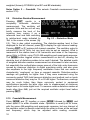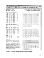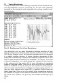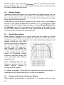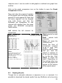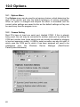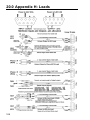
1
Lindos MS20
Audio Test Set
User Manual
Second Edition
Written by Chris Skirrow & Pete Skirrow
© Lindos Electronics 2010
1
Contents
1.0
Introduction
1.1
1.2
1.3
1.4
1.5
1.6
1.7
1.8
1.9
2.0
3.0
4.0
2
Getting Started
Graphic Display
Power On/Off
Battery Indicator / Auto-Switch-Off
Reset
Non-volatile Memory
Configuration Options
The ‘Line-Up’ Sequence
Technical Support
6
6
8
8
9
10
10
11
11
12
Manual Operation
13
2.1
2.2
2.3
2.4
2.5
2.6
2.7
2.8
2.9
2.10
2.11
2.12
2.13
2.14
2.15
2.16
2.17
13
13
14
14
14
15
15
15
16
16
17
17
18
19
19
19
20
Monitor Volume
Generating Tones
Measuring Tones
Channel Selection and Mute
Programmable Presets
Measurement Options
Level Measurement
Noise Measurement
Distortion Residue Measurement
Crosstalk Measurement
Frequency Measurement
Phase Measurement
PPM (Peak Programme Meter) Use
Normalising
Range Changing
Manual Reference Setting
Microphone Use
Sequence Testing
21
3.1
3.2
3.3
3.4
3.5
3.6
3.7
3.8
3.9
3.10
3.11
3.12
3.13
3.14
3.15
3.16
3.17
22
23
24
24
24
25
25
25
26
26
27
27
28
28
29
30
31
Running a Sequence
Page Mode
Graphical Results
Frequency Response Graph Normalisation
Storing Results in Memory
Input Level
Direct Trigger
Choosing Sequences and Segments
User Defined Sequences
Inter-working with the LA100
Sequences Limitations
Normalising In Sequence Mode
Tone-burst Testing of PPMs
Time-Delay (Path Latency)
Tone-burst Testing to ITU-R (CCIR)-468
Standard Sequences (v1.0 firmware)
Segments Available (v1.0 firmware)
Digital Equipment Testing
32
4.1
34
Testing CD Players
4.2
4.3
4.4
5.0
6.0
7.0
8.0
9.0
Testing Computer Sound Cards
Testing MP3 Players
Testing A/D and D/A Convertors
35
37
40
Analogue Equipment Testing
41
5.1
5.2
5.3
5.4
5.5
5.6
5.7
5.8
41
42
44
47
48
52
54
55
Coping with Consumer Equipment levels
Testing Analogue Tape Machines
Testing Compact Cassette Decks
Testing Power Amplifiers
Testing Loudspeakers
Testing Headphones
Testing Microphones
Testing Microphone Inputs
Broadcast Testing
56
6.1
6.2
6.3
56
57
58
Special Level Considerations and Pre-emphasis
Recording Through the MiniSonic
Testing PPMs and other Program Level Meters
Lin4WinXP Support Software
60
7.1
7.2
7.3
7.4
60
60
60
61
Introduction
Installing the Software
Connecting the MS20
Basics
Sequence Handling
63
8.1
8.2
8.3
8.4
8.5
8.6
8.7
8.8
8.9
8.10
8.11
8.12
8.13
8.14
8.15
8.16
63
64
64
64
65
66
67
67
68
69
71
73
73
73
74
74
File Handling
Results Display
Results Manipulation
Comparing Frequency Response Graphs
Reading Results
Running MiniSonic Sequences
Creating User Sequences
Large Graph Display
Tolerance Testing
The Tolerance Definition
The Lindos Quality Grading Scheme
Printing Results
Displaying Multiple Results
Exporting Results via the Clipboard
Saving Graphs
Saving Results as HTML
Control Panel
75
9.1
9.2
9.3
9.4
9.5
9.6
9.7
9.8
9.9
9.10
75
75
76
76
76
76
77
77
77
77
Overview
Measurement Options
Setting Frequency and Level
Frequency and Level Presets
Setting the Output Channel
Keyboard Shortcuts
Frequency, Phase and Level Measurements
Distortion Measurement
Zoom Button
Reset and Close Buttons
3
9.11
9.12
9.13
9.14
10.0
12.0
13.0
14.0
15.0
77
78
80
81
Options
82
10.1
10.2
10.3
82
82
83
84
85
86
86
88
88
10.4
10.5
10.6
11.0
Saving the Panel Settings
Procedure Testing
Other facilities
Bar Graph Speed
Options Menu
Comms Setting
Graph Options
10.3.1
Graph Options: General Tab
10.3.2
Graph Options: Frequency Response Tab
10.3.3
Graph Options: Other Tabs
Results Format
Save Options
Tolerance Options
Other Features
90
11.1
11.2
90
90
Command Window
Tone Bursts
Uploading to the Test Results Database
91
12.1
12.2
12.3
91
92
92
Introduction
Creating an Account
Uploading Test Results
Appendix A Troubleshooting
94
13.1
13.2
94
94
Lin4WinXP Problems
No Oscillator Output
Appendix B - Firmware Updates and New Features
95
14.1
14.2
14.3
95
95
95
New in V6.03
New in V6.04
Firmware Updates
Appendix C Lin4WinXP File Formats
96
15.1
15.2
15.3
15.4
15.5
15.6
15.7
15.8
96
96
96
97
98
98
99
100
Sequence and Tolerance Files
Results Files
Results Header Lines
Results Text
Graph Handles
Packet Data
The Graph Packet
The Tolerance Packet
16.0
Appendix D Key Shortcuts
102
17.0
Appendix E: ‘468-Weighting’
103
18.0
Appendix F: Crosstalk Weighting
105
19.0
Appendix G: ‘UniSon’
106
20.0
Appendix H: Leads
108
21.0
Appendix I: Remote Commands
109
21.1
4
General Purpose Commands
109
21.2
21.3
22.0
Appendix J: Specifications
22.1
22.2
22.3
23.0
General
Oscillator
Analyser
Appendix K: Calibration Checking
23.1
23.2
23.3
Index
Oscillator Commands
Measurement Commands
Self-Test
User Calibration
Removing Battery and Case Top
109
109
111
111
111
112
114
114
114
115
116
5
1.0 Introduction
The first time user should read this chapter, which provides a ‘Getting
Started’ tutorial and describes the basic features of the unit, but may then
proceed to chapters 2 or 3 for a complete introduction to manual or
sequence measurement. Sequence testing is a very easy way of making a
predefined sequence of measurements, at the press of a few keys and
without any programming effort.
The MS20 is a complete portable audio test set that combines the functions
of an oscillator (signal generator), level meter, peak programme meter, noise
meter and distortion meter, along with frequency, phase, path latency and
tape speed measurement, in one small hand-held unit that can be used on
its own or with a computer by running the Lin4WinXP support software
provided.
The MS10 provides the same measurements as the MS20 but presents
them on a bar graph LED display. The MS1 is simply an MS10 with
sequence reading disabled (except for a sweep), sold at a price that is more
affordable by schools and enthusiasts. As sequence generation is not
disabled, it can also function as a low-cost generator for use with the
MS20/MS10 or LA100. The MS1 is easily upgraded to an MS10 by
purchasing a firmware upgrade. The MS10 can also be upgraded to an
MS20 by replacing by front panel.
1.1
6
Getting Started
• Connect the Osc (output) and In (input) sockets together, using the
UniSon to XLR leads provided, and set the MIC/LINE toggle switch
to LINE.
•
Switch the unit on with the top right-hand toggle switch and check
that the display lights up. The unit will power-down (into ‘sleep’
mode) if no key is pressed for 5 minutes: press any key to restore
operation.
•
Turn up the volume with the VOL slider and you should hear a 1kHz
tone. The speaker always monitors the left channel in level mode,
but is switched to the selected channel for noise, distortion etc. The
output is set to 1kHz at 0dBu on both channels and both level and
bargraph readouts display 0dB. The measured frequency and phase
are displayed to the left of the level readouts.
•
Hold down and press or to change the oscillator
frequency. The text ‘Osc Freq’ and the current output frequency will
appear on the display in place of the measured frequency and
phase. Hold and the key to change the frequency in finer
th
1/12 octave steps. Hold and press or to change the
output level (1dB steps). Hold and for 0.5dB steps.
•
Press . The oscillator automatically mutes and the reading
drops to around -82dB. You are now measuring the noise level of
the MS20’s oscillator output. Press or to select either channel.
•
Press . The unit will momentarily normalise the level, and then
display relative distortion (ITU-R 468 weighted quasi-peak).
•
Press to enter sequence mode and press to display a
list of pre-defined sequences, highlight ‘Broadcast Test’ using the
and keys and press menu again to run the sequence. Note
the audible FSK signal at the start of each test segment, which
signals the start of the measurement and the segment type. Once
the test has finished the unit will automatically switch to page mode
and display the results for the sweep segment. Use the and keys to move the cursor up and down to read off the stored levels.
As you have a simple direct connection the levels will be the same at
all frequencies. Press to step through the results for each of
the test segments. Pressing in page mode brings up another
menu that allows up to 3 sets of results to be stored and retrieved
from flash memory.
•
Press again to return to sequence mode and press and hold
key for 2 seconds to bring up the sequence editor. Use the and keys to select a segment and and to move
the cursor along the list. Press to return to sequence mode
and save the new sequence, then press key to run the sequence.
Another user-defined sequence can be setup on preset key .
•
Install Lin4WinXP on a PC (click on the CD drive and then
double-click on the ‘setup.exe’) and connect the MiniSonic using the
RS232 cable. Start Lin4WinXP (from Start/All Programs menu). The
control panel will open and a status bar at the bottom left should
show when connection has been established. If the box keeps
flashing red you may need to change the COM PORT setting
(Options/Configuration Options). You are now ready to play with the
many features of the control panel which are largely self-evident.
•
Press on the unit followed by and again to run
the Broadcast test. This will run a 20-second sequence of segments
(n,u,r,q,z,h) and on completion you will see full listings, with graphs,
appear in the results window in Lin4WinXP. Note that you can
double click on both the text and the graphs to bring up options and
an expanded graph with cursor readout. This demonstrates the full
7
power of sequence testing, which for many purposes may be all that
you need to use. You can now experiment with running other
sequences, either from the keys, or by entering any sequence of up
to eight segment letters (but note restrictions) in the text box on the
control panel under the RUN button. MiniSonic segments must be
entered as lower case letters as some LA100 segments also run on
the MS20. Press Return or click RUN to start the sequence.
•
To save results use the shortcut CTRL-S. To open a saved file use
CTRL-O or drag and drop the file icon into the main window. You will
have to specify directories for saving in the usual way, and it is a
good idea to create a ‘Results’ directory first. Note that tolerances
and comments can be added.
You are now ready to test a piece of actual equipment. In some cases this
will require both the input and the output to be connected to the MS20. In
others, such as when testing a sound card output or a CD player, only the
input of the MS20 will be connected, the test signal coming from recordings
of test sequences or tones which are available as downloads from
www.lindos.co.uk.
What follows is a detailed reference guide to the various functions of the
MS20 but you may find it more useful to skip to Section 4 for full details of
Sequence Testing, or Sections 9,10,11 which explain in detail how to test
various specific types of equipment.
1.2
Graphic Display
The full-graphic OLED (organic light emitting diode) display in the MS20
combines great flexibility of display with very low power consumption.
OLEDs differ from other displays in being able to provide a constant high
contrast over the entire viewing angle of 180°, both horizontally and
vertically. In dim light the default brightness setting may be found to be too
bright, but this is easily changed (see section 1.7). With the brightness set
to maximum, the display is perfectly useable out of doors, even in bright
sunlight.
1.3
Power On/Off
The unit can be powered externally using a 12V mains adapter or from a
rechargeable lithium-ion battery. The toggle switch controls the battery
power, but not the external power, and the unit will turn on as soon as
external power is applied. This is to facilitate use in fixed installations as a
PPM, alignment tone generator etc. Switching the toggle switch on with
mains power applied provides battery backup in the event of a mains power
failure.
8
The lithium-ion battery is supplied fully charged and will power the unit for
around 13 hrs, depending on the brightness configuration setting used. The
lithium-ion battery charges whenever external power is connected, the
charge rate reducing to zero as full charge is approached so that continuous
use on external power will not degrade battery life. External fast-charging
using a camcorder battery charger is also possible, as is the use of larger
capacity batteries that are available with compatible (Sony) fitting (versions
with or without ‘info-lithium’ are suitable).
Lithium-ion batteries normally retain charge for at least a year, even when
they are several years old (expected life is over ten years), and are internally
protected against over-discharge etc. Operation from a PP3 Alkaline battery
is possible (5hrs intermittent use) (request adapter lead from Lindos or use a
diode in series to prevent explosion through charging!) A PowerBus for
external microphone preamps and other devices is provided on pin 5 of all
input and output (UniSon) sockets. This is at 6 - 8V, (for regulation to 5V in
the device) current limited at 1 - 1.5A for safety (sometimes this pin may be
accidentally grounded by contact with the connector shell as it is inserted, in
which case the unit will be seen to reset due to brief loss of power). Powering
the MS20 via the UniSon PowerBus, without a battery, is also possible.
The power connector is 1.6mm centre positive and protected against reverse
polarity. Current consumption is 150mA, but rises to 350mA when charging a
flat battery.
1.4
Battery Indicator / Auto-Switch-Off
If no key is pressed for 5-minutes the unit will automatically enter ‘sleep’
mode and the display will turn off. Press (don’t tap) any key to restore
operation from sleep mode. Battery life in sleep mode is over 1000hrs and
both the working state and the complete state of the unit is retained in
RAM. Using the toggle switch to turn the unit on and off will save battery
life and ensure total reset, but any results in RAM will be lost, though they
can be saved to non-volatile FLASH memory for permanent storage (see
section 3.5). To put the unit into sleep mode press keys and together. If any external devices are taking power from the ‘UniSon’ input
or output connectors this is not turned off in sleep mode – toggle the power
off to avoid a flat battery.
When mains power is applied, sleep mode is automatically disabled. Note
that since this is achieved by sensing whether the voltage is above 8.1V,
auto-turn-off is also disabled on a well-charged battery. The sleep timer
can also be permanently disabled by setting the appropriate configuration
option (see section 1.7).
9
All main modes (LEVEL – SEQ) display a battery voltage indicator in the
top right corner of the screen. On a fully charged battery (8.3V) the four
bars inside the outline of the battery should be fully lit. As the battery
discharges these bars progressively dim and turn off. The unit will cease to
operate when the battery voltage reaches 5.5V.
1.5
Reset
Pressing and together resets
the unit to start-up conditions. The
display turns off and then
monetarily displays the start-up
screen (fig 1.0). Note that the serial
number of the unit and the firmware
version are displayed at the bottom
of the screen. The oscillator output
Fig. 1.0 – Start-up Screen
resets to 0dB, 1kHz, and level mode
is set. The sequence data and results listing stored in RAM are cleared.
Using this facility minimises mistakes caused by unwanted settings not being
cleared. Some settings are deliberately not cleared by a reset, e.g.
configuration options, user sequence definitions and presets. Note that if
configuration ‘Start-up Sequence’ is set then the oscillator will output the
selected sequence and PPM mode is set.
Continue to hold the key after performing a reset or a switch on to display
the start-up screen until the key is released.
1.6
Non-volatile Memory
The unit is equipped with non-volatile memory and the frequency and level
presets, measurement options, configuration settings and sequence
definitions are all kept, regardless of whether or not the unit is powered.
Sequence results can be written to and read from flash memory (see
section 3.5), but automatic storage is not currently provided.
Units are supplied in the default condition, but the user should be aware
that accidental setting of non-volatile functions could cause confusion. In
case of doubt, a complete reset will restore Lindos default settings. Press
and and a menu will appear with the following options:
Reset All
Reset Options
Reset Configurations
Reset Sequences
10
Press and the unit will be restored to normal operation, alternatively
a partial reset can be obtained by using the and keys to highlight the
required option and then pressing .
Exit the menu by pressing any of the main function keys ( – ).
1.7
Configuration Options
Press and to bring up
the configuration options screen
(fig 1.1). It offers to possibility of
changing various parameters such
as brightness, auto-switch-off time
and
the
startup
sequence
generated at switch on. A full list of
the options is provided below:
Sleep Timer
Lineup Sequence
Direct Trigger
Brightness
dBSPL mode
Startup Level
Startup Frequency
Fig. 1.1 – Configuration Editor
5 mins,10 mins, off
GLITS, Channel Ident, Lindos Lineup, off
off, on
0,1,2,3,4,5,6,7
off,on
Preset 1, Preset 2, Preset 3, Preset 4
Preset 1, Preset 2, Preset 3, Preset 4
Default options are shown in bold.
When the configuration options are displayed the right hand pair of up down
keys cycle through the configurations while the left pair select the option. The
right hand pair of keys auto repeat when held. Exit the menu by pressing any
of the main function keys ( – ).
1.8
The ‘Line-Up’ Sequence
A special, repeating, ‘line-up and channel-ident’ sequence can be generated
at power switch-on by selecting the required sequence using the ‘Line-up
Sequence’ configuration option as described above. This allows fixed use of
the MS20 as a line-up generator in broadcast applications. Line-up
sequences are often recorded at the start of programme material as
confirmation of alignment level and channel assignment for broadcasting. We
recommend using the ‘Lindos Line-up’ (segment j) sequence, which
increases the level to +8dB on the left channel first, then on both channels. It
combines the ability to identify left and right channels heard together or in
isolation, with a check of max level (PPM6 is +8dB). See section 3.0 for
11
further information on the channel ident segments.
Note that when a line-up sequence is selected the unit starts up in PPM
(Peak Programme Meter) mode. Press to stop the sequence. If the
‘Line-up Sequence’ configuration is set to ‘off’ the unit will start in Level
mode.
1.9
Technical Support
Lindos takes great pride in the technical support offered to its customers,
which includes free firmware updates and Lin4WinXP updates. Our
telephone support line (+44(0)1394 380307 is manned 9am-5pm GMT and
we aim to reply to technical queries sent by fax or email on the day they
are received (fax: +44(0)1394 385156, email: [email protected]).
Support is also available through our worldwide distributors network
although complex queries are best sent directly to Lindos. To help us
support you please ensure that you always supply your serial number and
firmware version in any correspondence – both are shown on the OLED
display when the unit is switched on or reset.
12
2.0 Manual Operation
The unit operates in manual mode when switched on, and can be toggled
between this and sequence mode by pressing . Any main key (
– ) can be used to exit from any other mode or menu and pressing
specifically performs a low level of reset, cancelling relative reading,
range settings and selecting both channels. The function keys are
particularly easy to use because they select a measurement to a predefined
standard, which is displayed below the function heading at the top of the
screen.
2.1
Monitor Volume
The speaker enables the measured signal to be heard at a loudness level set
by a small slider VOL control on top of the case. Only the left internal
channel is monitored in level or PPM modes. Plugging in headphones
disables the speaker and allows high-quality listening in stereo. In other
modes the speaker monitors the selected channel and is often useful
because it enables the nature of noise or distortion residues, or the progress
of a sequence test to be heard.
2.2
Generating Tones
Oscillator
setting
is
best
demonstrated in level mode, though
it works in other modes. Hold while operating the and keys
to change the frequency in thirdoctave steps from 4Hz – 40kHz.
‘Osc Freq’ and the currently selected
frequency will be displayed in place
Fig. 2.0 – Oscillator Frequency
of the measured frequency and
phase readouts (fig. 2.0). Hold and , to change the frequency in
twelfth-octave steps, but note that the oscillator frequency readout continues
to show the IEC third-octave frequency until the next third-octave is reached.
Release the key to view the measured frequency.
Hold while operating the and keys to change the level in 1dB
steps between -99dB and +19dB. Hold and , to change the level in
0.5dB steps.
13
2.3
Measuring Tones
The MS20 displays stereo signal
level,
frequency
and
phase
difference readouts when switched
on (fig. 2.1), and displays the level
of both channels on bar graphs as
well as the numerical readouts. The
four function keys select the
measurement, as described in
Fig. 2.1 – Level Mode
sections 2.7 - 2.13. Crosstalk
measurement is available on noise option 2 (hold and press )
and various miscellaneous measurements are available as options in PPM
mode.
The measurement range extends from -66dB to +19dB in level and PPM
modes and the lower limit extends to -84dB in noise and distortion modes.
All measurements are autoranging; the bar graph scale changing in 10dB
steps when the reading moves outside ±6dB of the centre. On wildly
varying signals though, manual range setting may be preferred, and
holding the key while using the and down keys changes the
range in 10dB steps. To re-enable autoranging just press the appropriate
function key or press twice.
2.4
Channel Selection and Mute
Press to silence the output. Press again to restore both channels (or
press ). Hold and press (or ) to output on the left or right
channel only. The current setting is displayed in the top-right-corner of the
screen next to the battery voltage indicator.
2.5
Programmable Presets
The two numbered keys to the left of the display give instant access to
preset frequencies and levels. If the oscillator frequency was last adjusted
then the keys operate as frequency presets, otherwise they operate as
level presets. A further two level and frequency presets can be accessed
by holding the or key respectively and pressing the preset key.
The presets are programmed by selecting the desired frequency or level
and pressing and holding the appropriate preset key or key combination for
two seconds. the text ‘Stored’ will be displayed as a confirmation message
until the keys are released.
The start-up level and frequency can be set to any of the four available
14
presets through the configuration options menu, see section 1.7.
2.6
Measurement Options
To select the measurement options for the current function, press and use the and keys to highlight the required option and press
. It is worth noting that the menu button works in most modes; to
provide access to sequences, configurations etc and all menus operate in
the same way.
2.7
Level Measurement
Level measurements use a rectifier with fast Quasi-Peak characteristics, not
true rms (root mean square). For most measurements, on sine wave signals,
this is of no consequence, and the readings correspond to rms value. The
term Quasi-Peak refers to any rectifier (detector) that responds essentially to
the peak of the signal, but takes a significant time to respond (integration
time). Increasing the input to a digital system beyond the clipping limit would
continue to produce an increasing output reading on a true-rms rectifier, as
the waveform became flattened, but a Quasi-Peak reading ceases to rise
abruptly at the rms sine-wave equivalent of the clipping level. This is a very
useful feature, made use of in the special headroom test segment ‘h’.
Level Option 1 – Fast Quasi-Peak level readings with frequency and phase
measurements.
Level Option 2 – Ultra-Fast Level (option 2). This selects level
measurement with a very fast response; reducing attack and decay times by
a factor of ten, which may be found useful when making rapid adjustments.
2.8
Noise Measurement
Readings are of absolute level
(relative to 0.775V), unless a test
level has been set in which case
readings will be relative to the test
level. To read noise relative to the
test level, press , wait a
second, and then press . This
is a convenient way to save the test
Fig. 2.2 – Noise Mode
level, which is the reading for the
current oscillator setting, as a reference level; a process called normalising
(see 5.3 for more details). Press to select the right channel; the MS20
includes only one set of measurement filters. Pressing (or )
restores left channel operation (fig. 2.2). The oscillator output is automatically
muted (though it can be de-muted) and measurements are ITU-R 468
15
weighted (formerly CCIR468-4 plus IEC and BS standards).
Noise Option 2 – Crosstalk. This selects Crosstalk measurement (see
section 2.10).
2.9
Distortion Residue Measurement
Pressing results in a
completely automatic distortion
measurement. The oscillator will
generate 1kHz and the unit will very
briefly measure the level of the
incoming tone, saving it as a
reference level and then switching
to relative-level mode indicated by
Fig. 2.3 – Distortion Mode
‘Rel’ in the corner of the screen (fig.
2.3). This is also called normalising. The distortion-residue level is then
displayed for the left channel, press to display the right channel reading.
Pressing or restores left channel operation. The oscillator output is
automatically set to 1kHz, but any level may be set as required. What is
measured is the relative level of all harmonics and noise in the frequency
range 2kHz to 20kHz, using ITU-R 468-weighting and quasi-peak response.
The button toggles relative measurement on and off, allowing the
absolute level of distortion-residue to be read if desired. The detailed merits
of weighted distortion-residue measurement are discussed in later sections,
but essentially the method takes proper account of the high order harmonics
caused by crossover distortion or digital quantising errors, and also gives
due emphasis to the high frequency modulation noise that can cause a
characteristic ‘roughness’ on tape or compact cassette. Distortion-residue
readings will generally be higher than if they were measured using the
commonly quoted THD (total harmonic distortion rms) method, and on harsh
crossover-distortion they may be 15 or 20 dB higher. Furthermore, readings
may be much higher than those commonly quoted in equipment
specifications because the latter often refer to measurement at maximum
output level or full scale digital level. To measure relative distortion residue at
levels other than 0dB, just set the required oscillator output level before
pressing .
2.10 Crosstalk Measurement
Press and together or press followed by and
select option 2 to enter crosstalk mode. Operation is exactly as for noise,
with the same 468-weighting and quasi-peak response, but one channel of
the oscillator output is always muted while the other is driven at the set level
and frequency, which may be adjusted while reading crosstalk.
16
Measurements are of absolute level, unless a reference level has been
saved by normalising (or previously pressing which normalises).
Crosstalk can be measured at any frequency or level, simply by changing the
oscillator settings, but note that the measurement is 468-Weighted, which
greatly emphasises readings around 6.3kHz (by 12.2dB). Use of the
automatic sequence test for crosstalk (segment ‘c’) is recommended as this
automatically changes the test level to give results that comply with a
standard originally devised by the IBA (Independent Broadcasting Authority)
for broadcast testing, with regard to both the (milder) IBA-recommended
weighting curve and the maximum permitted levels that apply where 50us
pre-emphasis is in use (such as on FM transmitters). See section 18.0 for
more information.
2.11 Frequency Measurement
The measured input frequency on the left channel is displayed in level mode
and is measured by timing zero-crossings over a number of cycles.
Readings are valid down to reasonably low signal levels (-30dB) where noise
starts to interfere. The frequency range is 4Hz to 40kHz, and aliasing will
occur above 40kHz (i.e. 50kHz will read as 30kHz).
2.12 Phase Measurement
Phase (between channels) is also displayed in level mode. Again, readings
are valid down to reasonably low signal levels (-30dB) where noise starts to
interfere. The frequency range is 40Hz to 40kHz. Note that the left channel is
considered the reference so that a +ve reading indicates that the right
channel leads the left and a –ve reading means that the right channel lags
behind the left. This was chosen because the left channel is used for FSK
signalling on sequences and so is the preferred channel to use as a directly
connected reference when measuring absolute phase in-out on a piece of
equipment. Phase difference between channels causes shifting of the stereo
image, and is a useful measurement to make when checking the azimuth
alignment of heads on analogue tape machines. There are circumstances
though in which the phase delay in a single channel is of interest, for
example when attempting to ‘time align’ separate drivers in a wide range
loudspeaker. In this case, the left channel input and output of the MiniSonic
should be connected directly and treated as the reference signal (by plugging
the XLR’s together or by making up a special lead incorporating the link. The
right channel input is then connected to the output of the device under test
(crossover network etc) so that what is displayed becomes the input-tooutput phase shift.
For microphone measurements a special trick can be used taking advantage
of the fact that when MIC is selected on the MiniSonic, the –ve UniSon inputs
17
remain functional and any input to them is summed with the Microphone
signal. A single wire connection between the –ve output and –ve input of the
left channel can therefore be used to provide a reference signal, allowing
absolute phase to be measured using a microphone plugged into the right
mic input. Do not attempt to use the standard XLR input lead to achieve this
(capacitive coupling in the lead to the floating +ve input will cause problems).
A D-type plug with a single wire to pin 1 (from pin 1 on the output connector)
is required (or Lindos can supply a special lead-set). Using such a set-up,
the microphone will show phase at a given distance from a speaker.
Alternatively it is possible to use two microphones and simply observe the
phase difference between them. This can be useful for checking the time
alignment of a sub-woofer for example, with one mic placed by the subwoofer and the other by the main speaker.
2.13 PPM (Peak Programme Meter) Use
Press , to display both
channels with accurate IEC (type Ilb
i.e. UK/BBC) dynamics. This mode
is ideal for checking the legality of
programme levels for broadcast or
recording. The range is set to 0dB
for use with standard broadcast
levels, but the input gain may be
Fig. 2.4 – PPM Mode
adjusted by holding down the key and using the and keys. While is held, ‘Gain’ and the gain
setting are displayed on the left of the display and gain settings from -50 to
+20dB are available. The LINE OUT UniSon socket provides a gaincontrolled output for recording purposes, with alignment level 0dBu out at
PPM4 (0dB on the scale). Selecting MIC on the toggle turns this mode into a
microphone recording set-up for voice-overs, location recording etc. Note
that +8dB corresponds to PPM6 or maximum permitted level for broadcast
material (EBU absolute max is +9dB), while 0dB is PPM4 or ‘normal’ level.
PPM Option 2 – Fast attack PPM provides an alternative PPM with very
fast attack (integration time of under 1ms) on both channels. Decay time is
as standard.
PPM Option 3 – Dual Speed PPM selects a dual-attack PPM operating
from the left channel only. The left bar retains standard PPM characteristics
while the right bar has the very fast attack of option 2. This will be found
useful for detecting whether brief peaks have been compressed. On
uncompressed live percussive sounds a difference of 5 to 15dB will be
observed between the two readings, as can be demonstrated by simply
plugging a Lindos miniature microphone into the left microphone socket,
18
selecting MIC, and banging two spoons together! This test demonstrates
convincingly why recording with realism requires 18dB or more of headroom
for the brief loud peaks that have little effect on perceived loudness (the ear
has a reduced response to brief bursts), yet are vital to maintain ‘sparkle’ on
percussive sounds. Using this mode to check recordings will reveal the
extent to which brief peaks have been limited or compressed. However, on
broadcasts and most recent CDs the two bars will rarely be seen to separate
by more than 1 or 2dB!
2.14 Normalising
Holding down the key for at least one second, while in level mode
stores the current input level as the reference level (and toggles to relative
reading as shown by the flashing indicator). The reading should therefore
jump to 0dB: if it doesn’t (as occasionally happens for big changes), just
press and hold again. All subsequent readings, in all modes, may be made
either absolute or relative to this stored level simply by toggling on or
off. This is most useful for relative noise readings at non-standard alignment
levels. For example: suppose that a CD player, playing the alignment-level
track of the Lindos test CD2 reads -2dB on level. Press and hold and
the reading changes to 0. Press , the reading is -65dB noise relative.
Press and the reading changes to -67dBu, which is the absolute
noise level. A quick way to read relative noise is simply to press , wait a
second, and then press , because distortion mode sets 1kHz and
normalises prior to reading distortion, and leaves relative reading set unless
it is cancelled by pressing .
2.15 Range Changing
On all measurement functions the measurement range can be changed in
10dB steps independently of any normalisation already applied, by holding
the key while using the and down. To re-enable autoranging just
press the appropriate function key or press twice.
2.16 Manual Reference Setting
The gain adjustment facility described under PPM actually works by
changing the reference level. It therefore provides a way of setting the
reference level in 1dB steps. This can be used as a sort of range changing
facility. The range of level and noise measurements can be extended using
this facility. For example, hold down PPM and use the up-down keys and set
the gain to +20dB. Now select noise and the readings will have increased by
20dB, permitting reading down to -90dB.
19
2.17 Microphone Use
Lindos microphones, are carefully calibrated by us (with a pair of selected
resistors in the gold-plated minijack) to produce a standard output of -30dBu
at 100dBSPL ± 0.5dB (UniSon Mic Standard). The MiniSonic’s microphone
inputs have a gain stage of 30dB resulting in the MiniSonic reading 0dBu for
100dBSPL (sound pressure level) at the microphone. Select configuration
option ‘dBSPL’ on the MiniSonic’s configuration options menu to read off the
true dBSPL readings. This simply adds 100 to all readings.
Lindos microphones can be used for loudspeaker testing, acoustic noise
measurements, and in matched stereo pairs for live recording. The MM3 is
extremely flat from 20Hz to 20kHz (typically +/-1dB) and is best used for
measurement purposes. The MM1 (Beyer MCE5.0) offers similar
performance to the MM3, but adds a small presence boost, making it ideal
for label use for interviews and voiceovers. The Beyer MCE60 offers slightly
lower noise than the MM1 and is to be preferred for applications such as
acoustic music recording.
When using the MiniSonic’s microphone inputs, ensure that the MIC toggle
switch is set to MIC and that nothing is plugged in to the normal D-type input
sockets. Where protective caps or windshields are supplied, these should
preferably be left off for measurements, as they can introduce 20kHz loss.
For more information on:
20
•
Loudspeakers testing see section 5.5.
•
Headphone testing see section 5.6
•
Microphone testing see section 5.7
•
Microphone input testing see section 5.8.
•
Recording through the MiniSonic see section 6.2
3.0 Sequence Testing
Lindos Sequence testing is a powerful innovation, first incorporated into the
LA100 in 1984 and universally used by broadcasters worldwide ever since. A
MiniSonic Sequence consists of up to eight segments; where segments are
like building blocks that can be chosen by the user. Each segment generates
a particular sequence of tones, a sweep, or silence, intended to test a
particular parameter, such as frequency response, distortion or noise. It
begins by sending its identifying character, (in ASCII code) as a frequencyshift-keyed (FSK 110-baud) signal which acts as a synchronising trigger as
well as the instruction for a series of timed measurements. This means of
course that the responding MiniSonic does not have to be the one generating
the sequence; it doesn’t even have to be on the same side of the world but
may be at the other end of a satellite link or line.
Because the measuring side of a MiniSonic unit operates quite
independently from the generating side, the signal may be delayed; by a
fraction of a second, as is the case when testing two-head tape machines, or
by years, as when playing back a tape that has had a sequence test
recorded on it for future quality checking. Any MiniSonic unit in sequence
mode will respond instantly to an appropriate FSK signal at its input, and go
into the appropriate series of measurements for the specified segment. At
the end of each segment it waits for up to one second for the next segment,
and when no more segments are detected it times out, switches to page
mode, and displays the results. If a PC running Lin4WinXP is connected, the
results will appear on the screen about a second after the sequence has
finished running, in the form of a Results Sheet that can be saved or printed
th
as an A4 page. Sequence 1 for example, will produce a 1/6 -octave plot of
frequency response, for two channels, in just five seconds. Sequence 3 will
produce a complete set of results, with graphs and bar charts, of frequency
response, relative phase, test levels, noise, and distortion at six levels, in just
20 seconds. Many other variations are possible by combining segments,
either by using the Sequence Editor (see section 3.9) or when using the
Lin4WinXP support software running on a PC (see section 8.6).
Up to three sets of results can be stored in the MS20’s non-volatile memory
to be viewed or transferred to a computer later. All sequence definitions are
preserved in non-volatile memory, so definitions need only be entered once.
21
3.1
Running a Sequence
17 ready-made test sequences are
currently available on the MS20, as
listed in section 3.16, these are all
constructed from test segments
listed in section 3.17. They differ in
the tests that are carried out and the
levels of the test signals used; each
being primarily intended for a
Fig. 3.0 – Sequence Menu
particular purpose. Press to
put the unit into sequence mode. The second line of text at the top of the
display indicates the currently selected sequence, which on startup defaults
to sequence 1. To run this sequence simply press again, to choose a
different pre-defined sequence press (fig. 3.0), select the required
sequence using the and keys and press . A sequence of test
segments is generated, and the message ‘Running Sequence’ will appear at
the top of the display. Assuming that a path exists to the input of the MS20
this will be responded to and ‘Logging’ followed by a list of letters denoting
receipt of the various test segments will be displayed. All segments make
measurements on both channels, and the sequence can be cancelled at any
point by pressing any of the main function keys.
When the tests have completed (typically 20s) the unit will automatically
switch to page mode and display the results.
All sequence levels are generated relative to the basic oscillator level set
prior to running them (0dBu unless altered). To ensure that this is 0dB, if in
doubt, reset the unit prior to entering sequence mode. In some instances, of
course, it will be desirable to run a sequence at a chosen level, for example
when testing low-level microphone inputs.
Most sequences start by generating a master-segment (n or m), which
begins with a test level segment, normalises to the measured level and then
proceeds to take noise measurements for both channels. Test level
segments cannot be run by themselves and are selected by the choice of
master-segment. The master-segments also measure path latency and
segment ‘m’ includes a tape speed measurement. Running a mastersegment (or resetting) clears existing results.
It is useful to remember that these basic sequences can be modified by the
subsequent running of certain segments, in particular segment ‘s’ (20s
sweep), segment ‘w’ (40Hz-40kHz wide band sweep), or segment ‘c’
(crosstalk). These are available in stand-alone use, and because a mastersegment is not run again they replace or add to the segments already run.
Where the initial sequence incorporated a normalising master-segment, the
added segments are also normalised. The ‘REL’ indicator will appear if
22
master-segment m or n is responded to, to indicate that relative reading is in
progress.
If a PC running Lin4WinXP is connected, then completion of the sequence is
indicated by the appearance of a results page on the screen.
Note that the FSK is only recognised on the left channel, and that it requires
a path that can transmit signals around 1.8 kHz. Use configuration option
‘direct trigger’ (see section 3.7 and 1.7) to test low-frequency-only paths,
such as sub-woofers or crossover filters. FSK operation means that another
MiniSonic may be used for measurement, even at the distant end of a line or
satellite link. Loudspeaker measurements can also be made conveniently.
In-car speaker responses may be measured, for example, by playing a
sweep segment from a test tape or CD (available from Lindos, or as a
download), with automatic triggering from the microphone signal so that no
electrical connection is required. Computer sound-cards and MP3 players
can be tested using downloaded test sequence files (available at
www.lindos.co.uk).
3.2
Page Mode
Once in page mode, the results of a previously run test sequence can be
viewed a screenful at a time by pressing to cycle forward through
the results in the following order: frequency response graph, phase
response graph, headroom plot, noise against time graph, test level and
noise, path latency and speed measurement, distortion (-20 to +8),
distortion (+12 to +18) and crosstalk.
Fig. 3.1 – Frequency Response
Fig. 3.2 – Noise Against Time
Fig. 3.3 – Phase Response
Fig. 3.4 – Level against Level
23
3.3
Graphical Results
The frequency response page shows a graph (fig. 3.1), usually covering
20Hz to 20kHz. The right channel trace is displayed with reduced
th
brightness. The cursor may be moved in 1/6 octave steps using the arrow
keys and , and the frequency and left and right levels (at the cursor
position) can be read from the numerical readouts at the bottom of the
screen. These readouts are derived from the stored 64 point graph data,
and provide much greater accuracy than can be inferred from the graph
directly. The left channel numerical readout is always the readout on the
left. Frequency response results are always normalised to 1kHz unless
normalisation is used, see section 3.4.
The noise plot (fig. 3.2), phase plot (fig. 3.3) and headroom plot (fig. 3.4)
cursors behave in the same way.
Note that the phase plot results are only valid above 1kHz.
3.4
Frequency Response Graph Normalisation
Select the frequency response graph display in page mode and press and
hold to normalise the graph to the left channel level at the
frequency selected by the graph cursor. Pressing toggles between
the normalised graph and the original graph. The level readouts shown
below the graph are not affected and remain normalised to 1kHz if a
master-segment (‘n’ or ‘m’) has been run or absolute if the sweep segment
is used without a master-segment.
Graph normalisation is useful for viewing graphs run at high or low levels
without normalisation (i.e. without a master-segment), and for inspecting
large level changes that are at the top or bottom of the graph.
3.5
Storing Results in Memory
Up to three sets of stereo
sequence results can be held in
non-volatile memory for later
viewing or transfer to a computer.
A menu (fig. 3.5) is obtained by
pressing when in page
mode. The top three options allow
transfer of the results in RAM to
24
Fig. 3.5 – Save/Read Sequence
flash memory and the bottom three enable recall of the results back from
flash to RAM. Select the required option using the and keys and
press . If a save option is selected then the unit will switch to
sequence mode in preparation for the next set of results. Selecting a read
option will cause the unit to return to page mode and display the saved
results.
3.6
Input Level
The MS20 looks for FSK signals at a nominal level of 0dBu, being primarily
intended for direct connection to professional line levels, but a wide range
of levels should give satisfactory operation (-30 to +18dBu). Below this
level the FSK may not be received, especially if the system is noisy, but
see below for details on direct trigger operation. The actual measurements
made by the segments use various ranging techniques and are
independent of the input level.
3.7
Direct Trigger
Selecting direct trigger mode from the configuration menu (see section 1.7
for further details) allows segment characters to be passed internally from
generator to measuring set, rather than by FSK (frequency shift keyed)
signalling over the measurement path. This is useful for testing devices
that attenuate frequencies in the 1650 to 1850Hz region used by the FSK,
such as sub-woofers, and crossover-filters. Sequence measurement
commences when a key is pressed to send the sequence or segment,
even if no signal path exists.
3.8
Choosing Sequences and Segments
Sequences 1 to 4 are ordered according to complexity (and time taken).
Sequence 3 is probably the most useful, as it tests most things in 20 secs,
but because it tests distortion with tones up to +18dB AL it is not suitable for
broadcast tests. Sequence 2, which only tests up to +8dB AL, is suited to
digital broadcast tests, but sequence 6, which uses less sensitive
measurement ranges on noise and distortion, and also runs the sweep at
-10dB is better suited to FM transmitter paths where pre-emphasis could
cause the system to be overloaded at high frequencies on a 0dB sweep.
Sequence 4 is sequence 3 with the addition of the 20 second noise plot,
providing a more thorough test of computers and devices that might have
occasional noise clicks.
25
3.9
User Defined Sequences
Many engineers find the Lindos default sequences are appropriate for
nearly all their testing requirements, but the ability to create two user
defined sequences with quick access on buttons and is provided.
These sequences default to segment ‘u’ on key and ‘nurq’ on key .
To edit a user defined sequence put the unit into sequence mode and then
press and hold the preset key. After two seconds the sequence editor
screen will appear displaying the current sequence definition. Use the
and keys to move the cursor through the sequence
definition, which is a single line of up to 8 characters. The and keys
change the character at the cursor and cycle through the available
segment letters.
To delete a segment character press and hold either or keys to
cycle through to the beginning or end of the character list. When either end
is reached the segment will be deleted and the cursor will move one
character to the left (unless the first character is deleted).
When the cursor is under a segment letter the segment title is displayed on
the bottom line of the display. Pressing any of the main function keys
( - ) will exit the sequence editor and save the new sequence
to non-volatile memory, ready to be run by pressing the appropriate preset
key from sequence mode.
Sequences should usually start with a master-segment (test level segment)
as this normalises and stores a reference level for other segments to use.
Test segments are indicated by a letter, A-Z or a-z, and the case is
important (u is not the same as U), all MiniSonic segments are lowercase
while LA100 segments are upper case. When designing a sequence you
should choose the measurement you want to include from the list shown
on page 31.
All sequences can be restored to their default definitions, using the reset
menu. Hold and to obtain the reset menu and select option 4.
3.10 Inter-working with the LA100
The MS20 normally uses segments that are different from those recognised
by the LA100, because its design made a faster and better set possible.
MiniSonic segments take advantage of the MS20’s ability to measure levels
on both channels simultaneously as well as its ‘smart-rectifier’ which
changes speed for fast settling on all measurements. The Distortion Residue
segments (q and r) in particular provide an informative set of weighted
26
distortion measurement at six different levels, which is not practicable on the
LA100 because of settling limitations.
To distinguish them from LA100 segments, MiniSonic segments are
characterised by lowercase characters (the LA100 uses mostly capitals).
They are only sent once, both channels being measured simultaneously on
sweeps, or in rapid succession during other segments (the LA100 sends
each segment twice, once for each channel).
Recognising that it might nevertheless be useful to use the MS20 in an
LA100 environment (especially on lines and links), a degree of compatibility
has been provided for generation and measurement of the most commonly
used LA100 segments. Further work is needed for the recognition and
logging of some LA100 segments to work reliably. Currently the MS0 will
time out on segments it cannot recognise, and is confused by some of the
sequences or text headers normally sent by the LA101. It is advisable to
delete any sequence titles from the sequence definition on the LA101. See
section 3.17 for a full list of supported LA100 segments.
3.11 Sequences Limitations
Any combination of segments (up to 8) can be sent as a sequence either
through the sequence editor (see section 3.9) or via Lin4WinXP, with the
following provisos:
•
Only one ‘master-segment’ can be sent (n or m)
•
Only one sweep segment can be sent (u, s, v or w)
•
Segment z must be run in conjuction with a sweep segment
•
Segment t used in place of segment m adds (azimuth)
alignment tones.
•
Segment q automatically runs segment r
Attempting to run LA100 segments alone will usually result in other segments
being run automatically. This is because the LA100 requires message text at
the beginning and a terminating character at the end. Segment ‘T’
incorporates the header text and also normalises. Segment ‘Z’ (phase)
incorporates the terminating character.
Segment ‘q’ actually tests distortion at +11.5, +14.5, and +17.5dB rather than
the nominal +12, +15 and +18dB quoted for simplicity. This provides a
margin of safety to avoid ‘just clipping’ when equipment is not precisely
aligned.
3.12 Normalising In Sequence Mode
It is usually advisable to include a ‘master-segment’ (n or m) in every
27
sequence as this automatically causes a reference level to be saved, and
sets relative-reading. This ensures that noise is measured relative to
alignment-level, and also that distortion segments operate within their optimal
signal level range, regardless of the actual level coming out of the equipment
under test, avoiding the possibility of front-end overload. Only the test level
results indicate the true level output from the equipment before
normalisation. Distortion measurements are made relative to the measured
level of the individual tone used.
If sweep or noise segments are run without a master-segment, then the
results will be absolute in dBu. This provides one way of altering the amount
of headroom available on sweep graphs. These normally limit at +10 and –
22dB which is plenty for normal use when testing nominally flat equipment. It
may not be enough though when testing filters or equalisers, in which case
running the sweep at, -5dB for example (reset the unit to cancel existing
stored test levels) will result in a graph with 15dB of ‘headroom’. Alternatively,
it is possible to run the sweep at normal level, but manually set the reference
level by holding and using the and keys . Press and run
segments in the normal way and they will be normalised to the manually set
reference level, provided that no master-seg is run. Running distortion
segments without a master-segment is not recommended.
Once a master-segment (n or m) has been run, the reference level it
acquired is applied to all subsequent segments, as indicated by the ‘REL’
indicator. If extra segments are then run, such as an alternative sweep or a
noise plot, then normalisation will also be applied to these. Running a
master-segment resets the reference level and clears the existing results list.
Resetting the unit also clears the results list, allowing segments to be run
without normalising if desired.
3.13 Tone-burst Testing of PPMs
Sequence 12 runs segment ‘p’ which is designed to test the dynamic
characteristics of PPMs (Peak Programme Meters). It does this by
generating five bursts of high frequency tones, of different durations and at
amplitudes designed to cause a correctly responding PPM to peak to 0dB on
each of them. See section 6.3 for more information.
3.14 Time-Delay (Path Latency)
Long signal paths, such as satellite links and long landlines, can introduce
a time delay of 100ms or more, enough to make conversation difficult. The
MS20 measures the delay on any return path by timing its FSK, and this is
listed in milliseconds as ‘DELms’ on Lin4WinXP results and as separate
‘Path Latency’ page on the display whenever a master-seg (m or n) is run.
Delays of 1ms to 10secs can be measured to an accuracy of ±0.05%
28
±1ms. Codecs (MPEG etc) also introduce delays, which can also be
measured to aid video synchronisation.
3.15 Tone-burst Testing to ITU-R (CCIR)-468
Segment ‘y’ works in exactly the same way as the PPM test, but is designed
to test noise meter dynamics to ITU-R 468 (CCIR) recommendation. Each of
the tone-bursts is designed to give a peak reading of 0dB on a properly
working meter, but this time the level is set for a target reading of -50dBu.
Note that the levels have been calculated to take account of the ITU-R 468
weighting filter response at the 5kHz burst frequency, so the test gives a
good measure of overall accuracy and freedom from overload limiting in the
most relevant region of the weighting curve. Tone-bursts are 1, 5, 10, 50,
100ms @ -46.3, -53.7, -55.3, -57.1, -58.4dB respectively (to nearest 0.5dB),
with 2.25s delays in between. All should hit 0dB on the scale (-50dBu).
29
3.16 Standard Sequences (v1.0 firmware)
Description:
Segs:
Measures:
SEQ0
‘Line-Up’
j
0dB/+8dB line-up/chan ident
SEQ1
‘Sweep’
u
sweep 20Hz-20kHz 5 secs
SEQ2
‘Broadcast test’
n,u,r,z
sweep, phase, noise, dist to +8dB
SEQ3
‘Digital test’
n,u,r,q,z,h
sweep, phase, noise, distortion, headroom
SEQ4
‘Sound-card test’
n,u,r,q,l,h,z
digital test plus 20s noise plot
SEQ5
‘Slow Sweep’
s
sweep 20Hz-20kHz 20 secs
SEQ6
‘Tape/FM test’
m,v,r,z
sweep @ -10dB, & high ranges
SEQ7
‘GLITS test’
g
channel ident and line-up
SEQ8
‘Wideband sweep’
w
sweep 40Hz-40kHz 5 secs
SEQ9
‘Headroom plot’
h
level versus level 0dB to +18
SEQ10
‘Long noise plot’
l
noise peak and mean 20 secs
SEQ11
‘Distortion segments’
r,q
distortion residue –20 to +18dB
SEQ12
‘PPM tone bursts’
p
5 ‘inverse-level’ tone-bursts
SEQ13
‘Crosstalk’
c
crosstalk at 100Hz 3.15k 10kHz
SEQ14
‘Sweep, phase, test level’ TUY
SEQ15
‘General’
TRINY
sweep @-10 phase, noise, dist
SEQ16
‘Digital test’
TUDNY
sweep @ 0dB, phase noise, dist
SEQ17
‘Broadcast test’
VRAGNY
sweep etc with 50us de-emphasis
30
sweep 20Hz-20kHz 5 secs
3.17 Segments Available (v1.0 firmware)
Name:
Description:
Details:
SEG n
Master-segment
Test lev/Normalise 1kHz /Noise (-85 to –50dB)/Delay
SEG m
Tape/FM Master-seg Test lev/Normalise 400Hz/Noise (-60 to –30dB)/Delay/Speed
SEG t
Test-Tape Intro
3.150kHz 8s,10kHz 8s,1kHz 8s, then as segment m
SEG u
Sweep
20Hz – 20kHz @ 0dB 5s
SEG v
Tape Sweep
20Hz – 20kHz @ -10dB 5s
SEG w
Wide Sweep
40Hz – 40kHz @ 0dB 5s
SEG s
Slow Sweep
20Hz – 20kHz @ 0dB 20s
SEG r
Distortion Residue
Distortion residue 1kHz @ -20, 0, +8dB
SEG q
Distortion Residue
Distortion residue 1kHz @ +12, +15, +18dB
SEG c
Crosstalk
Crosstalk at 100Hz, 3.15kHz, 10kHz @ 0dB IBA-wtd
SEG h
Headroom Plot
1kHz 0dB to +18dB in 1dB steps 5 sec plot
SEG l
Long Noise Plot
Noise weighted 468 (-85 to -50dB) left channel 20s plot
Special Purpose Segments:
SEG p
PPM Tone-burst test
SEG y
468-Wtd Tone-bursts ‘Inverse Tone Bursts’ 1, 1.5, 5, 10, 100ms
‘Inverse Tone Bursts’ 1, 1.5, 5, 10, 100ms
SEG b
Tone-bursts
General Tone Bursts 100, 10, 5, 1, 0.5ms @ 0dB
SEG e
Flutter Cal Wobble
Flutter-meter cal wobble (should read 1.1% IEC wtd)
SEG f
Flutter Test
3.15kHz 20 sec (provisional - not yet recognised)
SEG i
Channel Ident
1kHz 0dB 1 sec, 1kHz –6dB 1 sec, repeating
SEG j
Lindos Lineup
1kHz 0dB L+R 2secs, +8 dB L 2s, +8 L+R 2s repeating
SEG g
‘GLITS’ test
1kHz –3dB 6s total 1 mute on L , 2 mutes R repeating
SEG z
Phase (FSK only)
Phase Plot (valid only above 1kHz) (Use with u,v,s, or w)
SEG/
Sequence Separator
Use in Lin4WinXP to separate multiple-sequence generation
SEG<
Repeat (<n optional)
LA100 Segments:
Use in Lin4WinXP to repeat indefinitely (<3 does 3 repeats)
(* = not currently logged by the MS20)
SEGT
Test Level 1kHz
1kHz @ 0dB (includes ‘LA100’ start text) 1 sec
SEGV
Test Level 400Hz
400Hz @ 0dB (includes ‘LA100’ start text) 1 sec
SEGU
Sweep
20Hz – 20kHz @ 0dB 5s
SEGR
Tape Sweep
20Hz – 20kHz @ -10dB 5s
SEGD*
Distortion (THD)
100Hz, 1kHz, 6.3kHz @ +8dB 6s
SEGG*
Distortion 50us
40, 100, 315, 1k, 6k3, 10kHz with 50us de-emphasis 18s
SEGI*
Distortion (THD)
100, 1kHz @ +8 and –10dB 8s
SEGA*
Crosstalk
40, 100, 315, 1k, 6k3, 10kHz with 50us de-emphasis 6s
SEGN
Noise
Mute for 8s
SEGW*
Wow & Flutter
3.150kHz for 12s
SEGY
Phase (and stop)
count)
40, 100, 1k, 6k3, 10k, 15k (includes LA100 stop and segment
31
4.0 Digital Equipment Testing
A selection of Lindos test Segments, and sequences, is available as MP3 or
WAV files for download from the www.lindos.co.uk website. These can be put
to CD or loaded into media players to test soundcards etc.
Although the MiniSonic is, at first sight, an analogue test set, it is capable of
testing the best 24-bit digital systems for noise and distortion down to the
lowest achievable levels. With a maximum output signal level of +19dBu and
an input residual noise level of -90dBu (468-Wtd) it has around 10dB more
‘dynamic range’ than the best digital systems, and some 30dB more than
most 16-bit systems. This demonstrates a major advantage of using an
analogue test set. No digital system capable of +18dBu output is likely to
achieve a noise level much below -80dBu (468-Wtd), so to compete in the
analogue domain it needs adjustable analogue gain switching. The figures
often quoted for digital systems, of 110dB or more of ‘dynamic range’, have
to be taken with a pinch of salt; they are usually measured unweighted or Aweighted rms, and relative to full-scale, and so are not directly comparable
with our subjectively valid measurements.
To test a purely digital piece of equipment, it is necessary to convert the
output to analogue using a digital convertor, and Lindos supply several
convertors for this purpose. There is a lot to be said for the concept of
regarding analogue as the fundamental domain, and conversion as part of
the set-up under test, for several reasons. Firstly, most equipment has
analogue inputs and outputs anyway. Then, the inputs and outputs may be at
different sample and bit rates, with different alignment levels; especially when
a complete path in a broadcast or studio environment is being tested, so it
makes sense to choose and set up each convertor accordingly. All real
signal chains start and end as analogue signal, at the microphone and
loudspeaker which are usually the weakest links in the chain. A purely digital
test set is therefore restricted in what it can test. In many situations where a
digital input is required, a test CD or digital test file can be the source. In
others, a CD player with suitable digital output can provide a convenient
source of sequence tests when used with a Lindos Test CD (CD2).
32
Fig. 4.0 – A Typical Results Sheet for a good CD Player
33
4.1
Testing CD Players
CD2, a Lindos Test CD, available from Lindos, or as a download at
www.lindos.co.uk (use a ‘Music’ CD-R when making a test CD – see later
comments), has been designed to facilitate the rapid sequence testing of CD
players. Unlike most test CD’s, this one has all levels referenced to
Alignment Level. A variety of sequences are provided, along with tones and
silence (with or without dither or noise-shaping).
Connect the MS20 using an appropriate lead, and press . Then play
Track 13 which will generate sequence 3 at -18dB FS alignment level, and
wait for the sequence to finish (by listening, or by watching for the results
screen to appear). Track 14 has been allocated deliberately as a mute track,
so that there is no rush to pause the player. When playing other tracks it may
be necessary to pause fairly quickly, or use the program facility on the player,
to avoid FSK-triggering by the next sequence.
A typical results page (see Fig 4.0) should show a Noise level of -65dB or
less. All sequence tracks on CD2 use noise-shaping rather than other forms
of dither to achieve the lowest residual noise floor, allowing very good
players to be distinguished. The +18dB Dist Residue should be reasonably
low (-50dB or less). The ‘Test Level’ figures in the results, show the deviation
of output level from the assumed UniSon standard. Consumer players
typically have a specified Full-Scale output level of 2V FS (+8.23dBu) which
corresponds to +14.23dB relative to the Unison alignment level. An
Alignment Level tone 18dB below this therefore gives rise to a Test Level of 3.68dB (14.32-18).
All tracks are duplicated at an alternative Alignment level of -15dB FS. While
-18dB FS is the main recommended EBU Alignment Level for studio
recordings (other EBU recommended levels are -12 and -24), there is a case
for using Track 3 (-15dB FS), rather than 13, especially when testing
consumer CD players, for three reasons. Firstly, it results in an output level
close to the UniSon standard (-6dBu) on typical consumer CD players.
Secondly, there is actually no recommended headroom figure for CDs and in
recent years recorded levels have been pushed ever higher in a rather an
attempt to make recordings sound louder. Thirdly, most items of consumer
equipment; camcorders, set top boxes, and PC cards especially, fall far short
of true 16-bit performance, so trading a little headroom for less noise, by
assuming an alignment level 15dB below FS for all ‘consumer’ equipment is
perhaps a good idea. If test files aligned at -15dB FS are used, the +18dB
Distortion Residue result is not valid, since the tone is already clipped in the
file.
CD-Rs ‘burnt’ on a PC often fail to play at all on standard CD players. This is
because of the different nature and size of the ‘pits’ made on a CD-R from
those on mass-produced (injection moulded) CD’s. The laser drives in PC’s
34
are set up differently, and have no problem reading either type of CD, but we
have found that even top quality CD-R’s have poor compatibility with many
music-only CD players. Usually, the problem is just a high error rate, which
the player is designed to conceal as far as possible, so a CD may sound fine
one day and then stop playing the next, because the error rate was only just
being coped with. To test for errors, play track 4 of the test CD (mute), press
and listen for clicks, which will often be heard at a rate of several a
second. A good CD will not have any clicks at all – they occur when the
powerful error correction in the player, which relies on redundant information,
cannot reconstruct the waveform perfectly and so resorts to ‘interpolation’ in
an attempt to mask the error. Interpolation is the reason why the clicks are
usually at a low level and not heard on music. Copying the test CD onto a
particular brand of CD-R is therefore a good way of assessing its suitability
for music recording, and keeping a CD-R that has a high error rate is a good
way of testing how tolerant a CD player is of pit variations. We currently use
Maxell Music CD-R’s, which claim to use a special dye, finding that they
really do work, giving no errors at all on a player that consistently fails to play
standard top quality TDK CD-R’s. This is not to say that the TDK CD-R’s are
inferior to Maxell of course – they may well be better for PC use, but there is
a compatibility problem with some players. Do not assume that all ‘music’
CD-R’s will solve this problem. Unless they specifically claim to improve the
laser reading on music players, including the word ‘Music’ may just be an
advertising ploy. It can also mean that the CD has a special pre-recorded
code or pilot track that is needed by certain stand-alone CD recorders, so
read the label carefully. Running segment l (long noise plot) is a good way of
testing for errors, which will show clearly as spikes. Errors are also audible
as clicks when measuring distortion residue.
4.2
Testing Computer Sound Cards
Sound cards, or onboard computer sound outputs present special problems
because, in general, they provide a multitude of ‘frills’, such as level, tone,
and balance controls. These often have bugs which are only revealed by
measurement, for example, a very popular soundcard gives well matched
output levels on both channels but then develops a 1dB channel difference
error forevermore once the balance control has been touched, even in the
central position! Such hidden problems can lead to all sorts of assumptions
about ‘subtle loss of stereo image’ in subjective tests, when in fact
measurement is revealing a simple fault. In an ideal world, it should be
possible to bypass all frills and work to standard input and output alignment
levels, and on a few ‘professional’ cards this is so. It should also be possible
to click on a ‘digital monitor’ button to put the A-D and D-A in cascade for a
simple in-out quality and level check, but surprisingly this easy-to-implement
feature is almost never present. In view of these and other deficiencies,
35
serious users are advised to treat mass-market cards that claim ‘24-bit 96k’
performance with scepticism, until validated by measurements. More basic
units with standard input and output levels and minimal controls, may give
similar performance, and a better chance of working with a known entity.
Sound cards should first be tested for playback (D-A) only quality and output
alignment level, by downloading a test file (sequence 3) from the Lindos
website (MP3 is fine) and playing it in a media player such as ‘Real-Player’
(available as a free download), or ‘Windows Media Player’ with the MS20 in
sequence mode. The results will usually be much worse than for a CD
player, though there is no fundamental reason why this should be so apart
from inadequate design. Most sound cards do not conform to any standard
with regard to input and output levels. Excessive noise is common, often the
result of general computer ‘hash’, or just analogue amplifier noise. Because
this noise is often introduced at the final analogue output stage, it will usually
be found necessary to have the output level slider set to maximum for
acceptable results, though there is no guarantee that this will not result in
clipping at full-scale level. If it does, a second run with the level turned down
should be tried.
Testing the input (A-D) performance is more difficult because of the need to
establish correct input alignment level by trial and error. It is important to
realise that most sound cards use a complicated analogue mixing scheme
such that monitoring the output directly gives no indication of digital
performance or level. It is therefore necessary either to make a recording,
using ‘RealRecorder’ for example, and play it back, or to use editing
software. The aim should be to establish the input level needed to produce
the same output as was measured at alignment level from the test file (the
‘Test Level’ figure in the result sheet), after which a sequence can be
captured at this level. An added problem though, is where to set the input
level sliders that appear in ‘Windows’. Setting them fully up will often result in
excessive input sensitivity and hence a large contribution of noise from the
analogue input circuits of the card and from hum loops in the input cable. Too
low a setting will result in front-end overload of the card prior to its analogue
gain control stage.
Most PC sound cards fail to achieve the (weighted) noise performance of
Lindos ‘Grade A’ (-60dB) even though this falls some 6 to 8dB short of
optimal ’16-bit’ performance. Another common failing, especially for on-board
computer sound, comes not from any subtlety of distortion or frequency
response, but simply from the lack of a proper ‘reconstruction’ filter, and
presents as audible beats or roughness on high frequency tones (5 to
15kHz). Any D-A convertor needs a low-pass filter after it to ‘reconstruct’ the
samples into the waveform they represent. The common assumption that this
filter is only needed to remove supersonic components that will not be heard
anyway is mistaken. High frequencies come out of a digital system
36
amplitude-modulated prior to reconstruction. They look like amplitudemodulated waves on an oscilloscope, and they sound either modulated or (if
the modulation frequency is high enough) ‘rough’. They may also have
higher than expected peak amplitude, which can lead to unexpected clipping.
The MS20 does not currently implement a test for this problem, so listening
carefully while slowly increasing the frequency in fine steps, or viewing the
waveform on an oscilloscope (or spectrum analysis) is recommended where
poor filtering is suspected.
Segment h (headroom test) may be found useful when testing cards with
unknown sensitivity. This produces a plot of output level versus input level in
1dB steps in 5 seconds, and clipping will be clearly seen as a flattening off of
the graph above a certain point. Because it is actually measuring the peak of
the sinewave (though reading rms equivalent) this test produces a sharp
flattening off of level that would not be apparent if the measurement was rms.
Segment l (long noise plot) may also be found useful, because audible clicks
produced when drives turn on or off, or buzzes as programs run, are often a
problem on PC sound. Playing a test CD on one PC was found to produce
clicks every second or so, at a weighted level 30dB worse than normal noise
level (Weighted Quasi-Peak measurement is designed to assess such clicks
according to audibility). The long noise test produces a 20-second plot (one
channel only) of noise, in addition to peak and mean (of the weighted quasipeak) figures, which gives a reasonable guarantee of freedom from clicks.
The best solution to the soundcard problem is to use a professional digital
convertor with SPDIF or AES3 digital connections to the computer, but even
this is fraught with problems, because some sort of ‘soundcard’ is needed to
get digital audio in and out of the PC, and once again the most popular cards
suffer a major defect. Though they do not reveal the fact, they actually work
internally at 48k (or 96k) sample rate, and use crude conversion for 44.1k
working. This can produce the surprising result of a frequency response with
±1dB ripple even when the convertor being used has no perceptible ripple –
again the sort of error that would be put down to other subtleties on listening
tests but is instantly revealed as a crude fault by measurement. Ripples in
frequency response of 1dB are not too important in terms of level change,
but may be audible as coloration because of the phase shift, time smearing,
and ringing they are likely to be associated with. Sample-rate conversion is
always undesirable unless absolutely necessary, and any form of digital
processing, even level adjustment, is likely to give rise to worsened noise
performance.
4.3
Testing MP3 Players
Test files are available at www.lindos.co.uk for free download in MP3 form.
Start with track 13, at -18dB FS which can be loaded into the MP3 player
37
over a USB connection, or in some cases copied directly to a flash memory
card. Some players appear in Windows as storage devices, others require
special software to be installed. The tiny portable players have output levels
around 20dB below UniSon level, and may only have a headphone socket.
Start with the volume set to maximum, and only reduce it if clipping is
suspected on the +15dB distortion result. Normalisation should take care of
the low level. Just press and play the sequence into the MS20 to
obtain a full set of results in Lin4Win. Erratic FSK triggering is usually an
indication of spurious supersonic output - inadequate ‘reconstruction’ filtering.
Players that use plug-in flash (usually SD) cards are very convenient,
provided that they work from standard MP3 files (some don’t), because a
card with sequences on it can be kept for testing and just slotted in.
Bandwidth limitation seems common in most MP3 codecs (Coder-Decoders),
and our test files, made using RealPlayer Gold, are typical, rolling off sharply
above 11kHz (96kb/s) and 16kHz (128kb/s and above). The AAC (Advanced
Audio Coding) option in RealPlayer extends to 20kHz. For MP3 testing we
therefore recommend using the128kb/s test file. On a good player this has a
noise floor around -64dB and distortion residues around –65dB, both
excellent figures. The use of higher bit-rates does not improve test results,
though by common consent 128kb/s probably generates artefacts on
program material that are occasionally just audible and can be reduced by
using higher bit rates. All codecs are not equal, so do not judge MP3 quality
at a given bit-rate without reference to the codec used; some early ones had
major defects.
A common problem with portable music players arises when EQ settings are
applied (jazz, pop, classical etc). Strictly the term equalizer is a misnomer as
there is no reason to equalise for different genres of music, but custom
settings can often be useful for applying bass, and possibly treble boost to
headphones. As this EQ is applied digitally within the 16-bit processing
system, high level signals are boosted out of range causing digital clipping
and thus high levels of distortion, especially on bass.
Where codecs are used for broadcast, for example in television sound, they
may introduce hundreds of milliseconds of delay, which has to be corrected
for by a matching delay in the video path. The MS20 measures path-delay
(latency) on sequence tests, from 1ms to 10secs (±0.05% ±1ms) and shows
it under ‘Test Level’.
38
Fig 4.1 A Typical Results Sheet for a good 24-bit Digital Convertor
39
4.4
Testing A/D and D/A Convertors
All of the above comments on measuring sound cards apply to Digital
Convertors, except that they are usually much easier to test because they
come with standard input and output alignment levels, and often with a
‘digital monitor’ switch. Where no such switch is present, it is easy to connect
the digital (AES3 or SPDIF) output and input together in order to make a
through measurement of input-to-output performance. Output-only (D-A)
performance can be tested using a digital (SPDIF or AES3) signal from a PC
playing downloaded Lindos test files (sequence 3 or 4). Alternatively, it may
be possible to feed digitally from a CD player (SPDIF or Optical) and use
Lindos Test CD (CD2) to play sequences.
While the lowest noise level obtainable from a 16-bit device is around -68dB,
24-bit devices might be expected, on purely theoretical considerations, to be
48dB better (6dB per bit). In practice, it is other factors like analogue noise,
sample and hold errors, and digital interference that limit the noise floor to
around -80dB (468-Wtd). Nevertheless this can be regarded as excellent
performance. 24 bits is a standard only because it fits the concept of 8-bit
bytes, needs no dither, and is potentially ‘better than we will even need’. It is
only really advantageous in recording situations where peak levels cannot be
anticipated accurately, because it allows recording at a low level (lots of
headroom) without adding to the noise floor of the microphone preamp.
Finished recordings, especially multi-tracked recording which necessarily
combine the noise from many microphone preamps will almost always have
a level of noise high enough to make the noise floor, even of good 16-bit
digital coding, irrelevant.
High sample-rate convertors (96 or 192 ks/s) can be tested for frequency
response using segment ‘w’ (40Hz to 40kHz sweep). This will reveal whether
the designer has chosen to roll off the response gradually above 20kHz for
minimal ringing, or rapidly at 40kHz.
Some convertors can occasionally function is a ‘partially locked on’ mode,
having failed to synchronise properly, perhaps on a change of sample rate.
Watch out for this, and other erratic failures of start-up as they can cause a
significant increase in noise which, though obvious on measurements, could
easily go unnoticed on programme material – a new hazard in the digital age.
40
5.0 Analogue Equipment Testing
Most professional analogue equipment can be connected using the XLR
leads, and tested without any adjustment of levels, as it is probably designed
to work at an alignment level of 0dBu (corresponding to the Lindos UniSon
standard). There is no such thing as ‘Full Scale’ in an analogue device
though, and while mixers and processors can be expected to work happily
up to +18dB or more, others, especially analogue tape machine may soft
limit without actually clipping at any particular level. Running segment ‘h’
(headroom) is a good way to establish if any limiting or clipping is occurring.
Press then and select the ‘Headroom plot’ test from the menu
(or enter ‘h’ into Lin4WinXP) and the resulting graph will clearly show the
transfer characteristic in 1dB steps.
5.1
Coping with Consumer Equipment levels
A special feature of the MiniSonic is its UniSon input circuit which gives twice
the gain when only side, (the +pin) of each input is connected, provided that
the other (the -pin) is left open circuit. Its UniSon output circuit, being centregrounded, also generates half the set level when connection is made to only
one side and ground. Using the phono leads supplied therefore, an oscillator
setting of 0dB will result in a signal level out of -6dBu, which in turn will result
in a measured reading of 0dB for a direct connection. In other words, if an
alignment level of -6dBu can be assumed for the equipment under test, and
Lindos supplied phono or minijack leads are used, then no further
attenuation or level correction is necessary – just proceed as for professional
equipment.
This is a neat concept, which Lindos is promoting as part of the UniSon
standard, offered on the Web in the hope that design engineers will consider
adopting it on all consumer equipment. As well as being conveniently half of
the professional level, -6dBu (388mV rms) is a sensible choice of Alignment
Level. In fact, many televisions and video recorders operate at around this
level, and some specify it (though without any proper definition in terms of
peak transmitted levels). A figure of -10dBV (316mV or -7.77dBu) is often
assumed for consumer equipment, though this has little meaning unless
defined with reference to permitted headroom. CD players are often specified
as giving 2.0V (+8.23dBu) out at FS (full scale) corresponding to an
alignment level of -6.77dBu with 15dB of headroom. The Lindos UniSon
standard of -6dBu AL (alignment level) is therefore a reasonable level to use
with a lot of equipment, especially if a test CD based on 15dB of Headroom
is used (the Lindos CD2 test CD has all tracks duplicated with 18dB and
15dB of headroom for this reason). Broadcast systems, such as NICAM and
Digital television, and Digital Audio Broadcasts (DAB) tend to use varying
41
amounts of headroom, and it would be a good idea if all set-top boxes, DAB
tuners etc were aligned to give -6dBu out for PPM4 (0dBu) at the studio-totransmitter feed. Miniature devices such as MP3 players, which are often
powered from a single cell, tend to give lower levels than standard, though it
would not be impossible to make them conform to UniSon.
The simple way to test consumer equipment is to assume an alignment level
of -6dBu (the UniSon standard) and see how much headroom results. Where
input and output level controls are provided on the equipment, it is a good
idea to adjust these for optimum performance at Unison level in and out, and
mark them for future reference. Other alignment levels can of course be
used, but remember that 0dB on the MiniSonic represents -6dBu both in and
out on the MiniSonic when single ended connections (such as phono or
3.5mm minijack leads) are used. See the UniSon articles in the articles
section of our website for further details on this concept.
5.2
Testing Analogue Tape Machines
The process of recording and replaying an analogue tape involves many
stages of ‘equalisation’ to compensate for the many factors that cause
deviation from a flat frequency response. The recording amplifier will usually
include a lot of high-frequency boost, mostly to compensate for ‘partial bias
erasure’ at high frequencies while the replay amplifier will essentially have a
falling 6dB/octave response to compensate for the fact that the voltage
induced in the replay head rises with frequency, being dependant on the rate
of change of flux. This makes standardisation between machines, very
difficult, and in practice standardisation is achieved by adjusting the replay
equalisation for a flat response from a carefully made test tape. Fortunately,
the replay performance of a tape machine is much more stable than the
recording side, but ideally this should still be checked using a commercial
test tape.
The first adjustment to make is of head azimuth, using a test tape that can be
assumed to have been recorded with a gap that was perfectly at right angles
to the edge of the tape. Mechanical adjustment of the head tilt, for zero
phase difference between channels, is made while playing a 10kHz to 16kHz
tone. Although phase difference causes shift of stereo image this is not the
main reason for the adjustment, because the ear only uses phase difference
as a directional cue below about 2kHz, where phase error due to azimuth
error will be insignificant. It is the loss of high frequency response caused by
azimuth error that is important, and even worse, the loss that results when
both channels are combined to give a mono signal (broadcast signals need
to be reproducible in mono without such loss). Phase difference is simply the
most sensitive measure of azimuth alignment.
The replay response can then be checked by playing a succession of tones
42
from a test tape and noting the level at each frequency. The tape speed can
also be checked by measuring a standard frequency track using the MS20
with Lin4WinXP, or by using the speed check option on a 3.150kHz
recording. Where a trusted reference machine is available, this may be used
to record a sequence (sequence 6) to produce a test tape for routine
checking, but reference to a lab-standard tape is ultimately desirable. Once
the replay characteristics have been established, record-replay tests and
adjustments can proceed. Most professional (2-head) machines can record
and replay simultaneously, which makes adjustment easy. Sequence testing
is ideal in this situation, because FSK triggering ensures that the time delay
between record and replay has no effect on the results. Frequency response
is best tested at -10dB AL (10dB below alignment level) on tape machines,
since their high frequency performance degrades above this level. Testing at
-20dB used to be recommended, but while this may give better results it fails
to show up severe restriction of high frequencies that can occur even at typical
levels on some machines. Attempts to equalise analogue tape machines at
0dB AL will usually result in over correction at low levels, making for too bright
a sound.
Sequence 6 is ideal for testing tape machines as it uses segment ‘v’ (sweep
at -10dB) and also the master-segment ‘m’ which modifies the noise and
distortion segments to use a higher range than normal. This enables it to
cope with the relatively high levels of distortion and that are to be expected
from tape. Segment ‘m’ also incorporates a period of 3.15kHz tone on which
tape speed is measured, which is only valid if the recording was made at
correct speed of course, and it uses 400Hz rather than 1kHz for the ‘test
level’ check – preferred because it falls below the region affected by any
equalisation errors. Analogue tape machines will usually have only 12 to15dB
of headroom, conventionally defined in terms of 3% third harmonic distortion.
Using the MiniSonic, the predominantly third order distortion component (at
3kHz) is emphasised by 8dB in the weighting filter, and high-frequency noise
modulation may add to this, so a figure of -20dB (10%) for Distortion Residue
is not unusual at high levels. This shows just how bad analogue tape is
compared to digital systems, when measured in the most meaningful way.
While the additional running of segment ‘q’ may provide useful information
about distortion at higher levels on some machines, segment ‘h’ is
recommended for a most revealing test of the overload characteristic up to
+18dB. This segment plots output level versus input level in 1dB steps, and
will usually reveal a gentle soft-limiting transfer characteristic with no definite
clipping point. It was this soft-limiting of course which made analogue tape so
forgiving of brief overloads when compared with the harsh clipping of digital
systems.
43
5.3
Testing Compact Cassette Decks
Compact cassette machines are tested in the same way as open reel tape
machines (see above), but because of the low tape speed and narrow head
gap, results are much less stable and more sensitive to head contamination,
tape type, head alignment and bias setting.Azimuth head alignment, the first
thing to check, will be found to be particularly problematic. The low tape
speed (4.75 cm/s) of compact cassette results in a wavelength on tape at
10kHz of about 5 microns (0.00475mm) so that an error in alignment of just
one micron between heads will cause 90deg of phase error. One micron is
th
very small indeed (1/25 of a hair-breadth), and maintaining this degree of
alignment between machines is almost impossible, with some surprising
results. A test cassette recorded on both ‘sides’, for example, may show zero
phase error on the machine that recorded it, yet show significant phase error
on one ‘side’ only, when played on another machine. How can this be? The
answer is that tape stretch takes place as the tape crosses the head, and if
the pressure applied to the tape across the head surface is not even, then
the tape will skew. This is of no consequence so long as the skew is always
the same, but different machines will have different head friction
characteristics and this will lead to different amounts of skew! Coupled with
this is another effect. The tape has to wrap round the head surface, which is
curved, to ensure contact at the gap. The distance travelled over the head
depends therefore on the length over which contact with the head is
maintained by the pressure pad, and if the pressure pad is not perfectly
square and uniform, skew will again result. There have been attempts to
market ‘reference shell’ cassettes, but they never succeeded in eliminating
these effects, and the real weakness of cassette was always its low tape
speed. We have discovered frequency response anomalies in testing
cassettes, which also appear at first sight to defy reason, and though they
may be of academic interest now, they are interesting in retrospect. Two test
tapes, each made on a Denon 2-head machine, with bias adjusted in each
case to optimise performance, were found to play back differently on another
(single head) machine (-5dB at 10kHz), though they played flat on the
Denon. A tape made on the second machine played back perfectly well on
the Denon, and in all cases azimuth misalignment was not the cause. How
can such ‘reciprocity failure’ exist? The answer seems to lie in the fact that a
two head machine usually uses a wide–gap recording head in order to
magnetise the tape more deeply than is possible in a single-head machine,
the aim being to get more signal off the tape and reduce relative noise. The
deeper magnetisation can be laid down at a different position – out of
44
Fig 5.0 A Typical Results Sheet from a Compact Cassette Machine
45
phase at high frequencies with the surface magnetisation, by an amount
dependent on bias level. This is of no consequence when played back with
the very narrow gap of a two head machine, which responds mostly to
surface magnetisation at short wavelengths, but can result in cancellation
between the layers when sensed by the wider replay gap of the single head
machine – hence the high frequency loss. The TDK SAX tape appears to
eliminate this problem because it uses two layers of different oxide, each
optimised for a different bias level. Magnetisation is laid down at the ‘exit
zone’ where the high-frequency bias amplitude falls to a critical value that no
longer erases the tape, and in normal tape this exit zone shifts with depth. So
there never was compatibility between cassette machines, no matter how
well they were set up, and how pre-recorded tapes really performed is
anybody’s guess!
A test cassette is available from Lindos, for checking replay response. It is
recorded with sequence 6, preceded by 8-second tones at 3.15kHz,10kHz
and 1kHz, to permit azimuth alignment and speed adjustment. If sequences
are recorded for use as test tapes it may be useful to use segment ‘t’ instead
of segment ‘m’ as the master-segment. This adds in the 8-second tones.
Note that special segment characters < and / can be used in Lin4WinXP to
generate complex test tapes. For example:
tvrz<4
repeats a tape test sequence ten times (with 8-sec tones)
tvrz<
repeats indefinitely
t/mvrz/mvrz/mvrz<10 sends tones, then 3 sequences, ten times
The special characters require that a path exists to enable the MS20 to
respond to its generated sequence, because Lin4WinXP waits until the
downloading of results is complete before continuing after the / or < symbol.
Record-replay performance is easily checked by running sequence 6, and on
two-head machines bias and record equalisation can be adjusted, either by
using fixed tones, for example to optimise the response at 10kHz, or
between sequence runs. On single head machines, it is necessary to record
the sequence, wind back, and replay, before making adjustments and trying
again; a process that was extremely tedious before sequence testing.
Typical results for a good compact cassette deck (chrome tape and Dolby B)
are -55dB Noise (468-Wtd) and -37dB Dist Residue at 0dB, though many
machines will fall short of these figures. Although it was primarily designed to
reduce noise, Dolby-B also reduces the audibility of modulation noise and
distortion products significantly. This can be particularly apparent on the
Distortion Residue measurement at -20dB.
46
5.4
Testing Power Amplifiers
The standard way to test power amplifiers is into a dummy load (8 or 4
ohms) but this needs to have quite a large heat sink capable of dissipating
the necessary power. It is also not representative of the actual load
presented by a loudspeaker, which contains reactive components
(inductance and capacitance), so the only truly valid way to test any amplifier
is with the loudspeaker that it is to be used with. If this is attempted, great
care should be taken to avoid overheating the drivers, especially tweeters;
limit periods of high level to a few seconds. Low to medium power amplifiers
can be tested at levels up to around 0.5 watt by connecting the MS20 input
directly across the speaker output, and this is best done using both pins
(differential input) because even though the speaker output and amplifier
input usually share a common ground connection, the high output current
involved is likely to cause ground voltage differences between input and
output, which may lead to feedback and oscillation at high frequencies if a
power amp’s input and output ground pins are connected together. Use the
XLR leads with an improvised connection into the + and – input pins (no
ground connection is necessary on the input – this is provided by the
oscillator output), or use a special lead. A good starting point is to set the
oscillator level and volume setting to produce 0dBu into the MS20 (0.775V
rms or 0.075 watts into 8 ohms. Run sequence 2 to obtain a complete set of
test results including distortion up to +8dB (0.473 watts into 8 ohms). Higher
levels than this necessitate the use of a special resistive attenuator on the
input, as otherwise the +12dBu input capability (unbalanced) of the MS20 is
exceeded. See section 20.0 for a diagram of a typical lead.
Power amplifiers have traditionally been accused of sounding different
because of crossover distortion, and huge efforts have been put into
reducing measured THD (rms total harmonic distortion) to ridiculously low
levels. This is an unscientific approach, because there is no level of THD that
can ever be said to be good enough. The many theories of how high-order
distortion should be assessed all seem flawed, because they attempt to deal
with the mathematically equivalent steady-state power spectrum without
recognising that our ears do short-term frequency discrimination. We hear
crossover distortion as a series of ‘clicks’ and a good tool for assessing the
audibility of clicks already exists in the ITU-R 468 weighted quasi-peak noise
measurement standard. Because it uses 468 weighting on distortion
measurement, the MS20 does a good job of assessing the actual audibility of
rd
crossover distortion. An amplifier with 0.1% (-60dB) of purely 3 harmonic
distortion will read 0.3% (-51dB) on the MS20 because the weighting curve is
9dB up at 3kHz. Another amplifier may measure 0.05% (-66dB) THD yet also
read 0.3% (-51dB) on the MS20, reflecting a harsher form of crossover.
Distortion residue below -50dB (0.3%) is probably inaudible, and below 60dB (0.1%) quite irrelevant.
47
5.5
Testing Loudspeakers
Speakers can be tested using one of the Lindos miniature microphones
plugged into one of the MiniSonic mic inputs. These inputs conform to the
UniSon-mic standard, with 5V power on the tip of the minijack and a
sensitivity of –30dBu (for 0dB on the scale).
The standard way to test a loudspeaker requires a fully anechoic chamber,
with an acoustically transparent floor-grid. The microphone is normally
mounted on an unobtrusive boom and positioned 1 metre in front of the drive
units on axis with the high-frequency driver. While this will produce
repeatable results, we would argue that more relevant measurements are
Fig 5.1 Results Sheet for a Monitor Speaker @2.5m in a Room
48
very easily made outdoors using the ‘half-space’ method described below.
Measurements made out of doors will usually show ripples in the mid-range
caused by ground reflections interfering. Raising both speaker and
microphone on poles has been used as a way of reducing ground effect, but
there is a much easier way: simply lay the speaker on its back pointing at the
sky. Ground reflection will still interfere, but will be greatly reduced in the midrange because most speakers are directional, and only radiate very low
frequencies backwards. Putting a folded quilt under the speaker will reduce
mid-range ripple by absorbing rear radiation. At low frequencies, the ground
reflection is always in-phase, so that the measured response will have
increased bass, but this is what generally happens in a room anyway, where
the rear wall and the floor both provide a similar effect. There is a good case
therefore for referring to the method as ‘half-space’ measurement, and
aiming for a flat ‘half-space’ response. Speakers that are equalised to give a
flat ‘free-space’ response, will always sound very bass-heavy indoors, which
is why they tend to incorporate ‘half-space’, and ‘quarter-space’ (for corner
use) options bringing in attenuation below about 400Hz. It makes more
sense, arguably, to design for half-space use in the first place, and only
boost the bass for open-air use! This method has been used to measure
known, very flat, speakers, with excellent results. Digging a hole and burying
the speaker flush with the ground should work even better, creating the
loudspeaker equivalent of the ‘boundary effect’ microphone (all reflections
precisely in-phase) but any rear port, must of course be kept open.
Measurements on a single speaker in a listening room, though less
satisfactory, can be interesting. At low frequencies, most rooms have
resonances at a series of frequencies where a room dimension corresponds
to a multiple number of half wavelengths. Sound travels at roughly 1 foot per
millisecond (1100ft/s or 350m/s), so a room 20 feet long will have
resonances from 25Hz upwards. These ‘resonant modes’ cause large peaks
and dips in response. A speaker in a room does not really ‘radiate’ low
frequencies at all, but couples into the ‘room modes’ – resonant standing
wave patterns. Because this coupling is impedance dependant, it cannot
even be predicted from measurements made of speaker radiation alone. Put
simply, some speakers present a very ‘stiff’ driving force and will drive a
resonant pressure peak at a boundary more efficiently than a ‘floppy’ one.
Dipole loudspeakers, such as electrostatics or ribbons, couple to the room
differently, by velocity rather than pressure, and are generally thought to
excite resonant peaks less.
All multi-driver speakers are prone to ‘suck out’ in the crossover region
between units (often around 3kHz) if the microphone is placed slightly above
or below the optimum axis, because the different path length from two drivers
producing the same frequency leads to phase cancellation. It is useful to
remember that, as a rule of thumb, 1kHz has a wavelength of 1 ft in air, and
49
10kHz a wavelength of only 1 inch. Published results are often only valid for
very precise positioning of the microphone to within a centimetre or two.
Measurements made at 0.5 to 1m are useful when it comes to speaker
optimisation, because at this proximity the radiated sound predominates over
reflections from walls, at least at high frequencies. Measurements made at 2
or 3m, in the actual listening position between two speakers can be much
more revealing of what is actually going on in a listening room. Horrendous
though the resulting frequency response may be, it provides a basis for real
experimentation with absorbent panels or resonators. Driving both speakers
is recommended, as this is the only way to stimulate low-frequency room
‘modes’ in a representative fashion – driving at one corner would be very
bad. This does mean though that the microphone must be positioned
precisely equidistant from the two speakers if a ‘comb-filter’ effect of alternate
peaks and dips is to be avoided. Positioning is best done by moving the mic
from side to side for maximum response on a 1kHz tone, then a 3kHz tone,
then a 10khz tone. Beware of applying carpeting or other thin absorbent
materials to large areas of wall in a listening room as this will result in an
unnaturally ‘dead’ room at high frequencies while having no effect on
reverberation at low frequencies. Glass-fibre or foam 100mm to 500mm thick
is necessary to damp down low frequency modes. An alternative approach to
low-frequency absorption is to space hardboard panels several inches away
from the wall, backed with glass fibre to damp their vibration.
Measurements at less than 1m will not allow proper combining of the
radiation from separate drivers around the crossover frequency. Even if the
path lengths are the same the tweeter will be ‘off-axis’. Very close
measurements can be useful though. Placing a microphone carefully on axis
a few centimetres in front of a tweeter will allow the high-end response to be
measured with minimal room effect. Similarly, placing one a few centimetres
in front of the voice coil of a bass driver will give some indication of how it is
responding (but not of the output from ports if these are present).
To minimise interference from ambient noise, the oscillator level and
amplifier volume can be set to give a reading of 0dB (100dB SPL), but this is
quite a high level, and should only be applied briefly (using the button
to turn the oscillator on and off) unless the system is known to be capable of
continuous drive at these levels. A level of 90dB SPL will be more
appropriate for smaller speakers. Ear defenders should be worn, as
exposure to continuous tones at high level can lead to hearing damage and
long-term tinnitus! Running sequence 1, a 5-second sweep will provide a
reasonable starting point, but sequence 5 (20-second sweep) is to be
preferred as it allows time for resonant modes to build up and decay, giving a
response curve with finer resolution and a more representative (if worse
looking!) result. For greater resolution when using levels below 100dB SLP
press and hold normalise first on a 1kHz tone, before running a sweep (or
50
set manual gain using PPM).
Automatic triggering of sequences from FSK via the microphone works
reliably in most situations, but in very reverberant rooms, or when measuring
sub-woofers, or bass drivers at very close range (with severe attenuation of
the FSK), use ‘direct trigger’ (see section 3.7). Two microphones, each very
close to a driver, can provide a powerful check of whether crossover filters
are really producing the phase shifts intended around the crossover region.
While the very best modern speakers can produce a frequency response flat
to +/- 1dB from 40Hz to 20kHz in anechoic conditions, measurements at 2m
in a real listening room can be considered good if they are within +/-12dB,
and efforts to produce anything like a flat response below 100Hz are likely to
provide endless scope for experimentation! This is where the real challenge
of audio quality lies, and having succeeded in building a listening room and
speaker set-up that is reasonably flat down to 20Hz we can testify to the fact
that a response flat to 30Hz content really makes a difference, while 20Hz
may possibly make a difference, mostly on bass-drums.
Using an equaliser to correct for room response is a poor solution, especially
at low frequencies, because it relies on reducing the drive at resonant modes
to produce a flat ‘steady state response’ once the resonant mode has built up
and stabilised, and this can take many tenths of a second. The result is
‘sluggish’ bass, because the initial wave-front has been greatly reduced by
the equaliser. Bass drums, and bass guitar, produce low frequencies with
sudden onset, and the initial wavefront accounts for much of the impact that
is both heard and felt. Realistic reproduction requires both the initial radiation
and the steady state level to have a flat response, and there is no easy way
to achieve this - room modes just have to be eliminated. The commonly
recommended approach of moving speakers around in an attempt to
stimulate the maximum number of modes is also not valid. It amounts to the
same thing as using an equaliser – adjusting the coupling of the speaker to
the mode as a way of controlling the steady state level, but at the expense of
the initial wave-front, with sluggish results. It should be clear from all this that
the concept of a ‘fast’ bass driver is utter nonsense. It is often claimed that
small bass drivers are ‘faster’, being able to accelerate more quickly. Yes, a
light cone is easier to accelerate, but this is only the same as saying that a
light cone can reproduce higher frequencies. Given that a driver can
generate a given frequency, its ability to generate higher frequencies; its
bandwidth, has little to do with the rate at which a low frequency tone builds
up or decays. Provided that the driver is operating at reasonably low ‘Q’ (a
feature of the driver plus its enclosure) then its contribution to the
sluggishness of bass response is likely to be negligible. This is less true of
reflex designs, though they remain popular simply because it is rare to find a
room in which their defects are not swamped by resonant modes.
Distortion measurements on speakers can only go as low as the distortion of
51
the measuring microphone itself of course, and for best results at high levels
(100 to 120 dB SPL) the MM2 is to be preferred. Although the MiniSonic only
normally measures distortion at 1kHz it incorporates a high-pass filter that
attenuates all frequencies below 2kHz (second harmonic) (-42dB @ 200
-59dB @ 100 -70dB @ 40Hz). This make possible a useful ‘Rub and Buzz’
test, over the 20 to 200Hz range. Just press and then vary the
oscillator frequency around the bottom end. The resulting quasi-peak
weighted measurement will ignore low harmonics, but give a good indication
of the high frequency residue that normally results from rattles, voice coil rub,
and hissing ports. Very few speakers can generate a pure 20Hz tone that is
not heard predominantly as hisses and buzzes, and this test has been used
on the production line of a major loudspeaker manufacturer.
It is interesting to measure actual listening levels on both live and reproduced
music in PPM mode (preferably super-fast PPM), because this captures and
holds the peak SPL (sound pressure level) demonstrating just how high peak
levels need to be for realistic reproduction without compression. A-weighted
readings, taken on a conventional sound level meter, may be much lower,
partly because A-weighting attenuates low frequencies, and partly because
rms levels imply a slow averaging process. A listening level of 100dB SPL,
measured A-weighted rms, might normally be considered very loud, but
100dB SPL on a PPM, though loud, is not excessively so, and still some 20
to 30dB lower than the level needed to achieve truly realistic comparison with
a live band. This is interesting because most speakers have a sensitivity of
around 86dB SPL for 1watt @1m, and so a level of 100dB SPL requires a
power input of 25 watts (10dB represents a 3 times increase in level, but a 10
times power increase because of the square law relationship). A typical topend speaker, driven by a typical 100watt amplifier, cannot therefore produce
peak levels much above 105dB SPL at 1m (which translates roughly to
105dB at listening position from a pair of speakers in a typical listening
room). Achieving truly realistic levels from such speakers would require peak
power inputs of at least 20dB more (100 time power) or 10,000 watts! The
use of bi-amped or tri-amped loudspeakers, where each frequency range
has its own amplifier, helps solve this peak-handling problem in a way not
often recognised, because peaks are usually the result of transient highfrequency bursts from cymbals, riding on sustained bass guitar notes.
Interestingly, two 100-watt amplifiers have the same peak handling ability as
a single 400-watt amplifier under such circumstances.
5.6
Testing Headphones
Headphones can be tested on the listener using a tiny mic tucked inside
close to the ear canal entrance. The Lindos MM4 (capsule only version of
MM3) is particularly suitable owing to its very small size. Set the volume for a
level of 0dB on the scale (100dB SPL)(or 90 and normalise) at 1kHz and
52
then run sequence 1. Most headphones feature a notch in the response
around 6-10kHz, which is often introduced by a reflecting plate (with holes)
mounted in front of each diaphragm. High frequency sounds originating in
front of us reach each ear canal greatly altered by head masking and pinna
(outer ear) reflections, an effect measured by so-called ‘head related transfer
functions’, or HRTFs. The notch is a crude attempt at the very complex
processing needed for proper headphone listening, which should ideally be
specific to each listener’s HRTFs. It reduces harshness when listening to
stereo recordings, though really there is no direct compatibility between
stereo and headphones. Bass is simply a function of pressure in the space
between headphone and eardrum, which is too small to add low frequency
resonances. Despite wild claims, like ‘frequency range 4Hz to 20kHz’, very
few headphones actually achieve even 40Hz to 1kHz +/-3dB and many only
seal effectively when held firmly against the head, which is not satisfactory.
Good ones give the same bass response with or without extra pressure.
Fig 5.2 In-Ear Response Plot for Top Quality Headphones
53
5.7
Testing Microphones
Testing Microphones is difficult challenge, especially where directional mics,
and large-diaphragm mics are concerned, but we have been pleasantly
surprised by the consistent results obtainable from various miniature omnidirectional mics.
Fig 5.3 Simultaneous Test of two Microphones
Omni-directional mics are easily calibrated for absolute sensitivity at 1kHz
using a small pressure calibrator, which typically produces a level of 114dB
SPL (Sound Pressure Level), but frequency response cannot be measured
in a sealed chamber because of severe chamber resonances at high
frequencies. The best way to measure the frequency response of a mic is to
strap a Lindos miniature measuring mic alongside it, on a boom, 1m in front
of a good loudspeaker, run a stereo sweep, and compare the two channels
of the response plot. See section 8.4 for more information on comparing
frequency response graphs. This can be done using the two microphone
inputs on the MS20, or even by using one mic input for the measuring mic,
and one normal input fed from an external mic preamp (using only the –ve
input pin which remains active when MIC is selected.) Avoid having any
object bigger than 10mm or so in the vicinity of the microphones and even
the presence of a larger mic will affect the soundfield in the vicinity of the test
mic. Small mics, however, can give very well matched results right up to
20kHz.
54
SPL is defined relative to 20uPa (micro pascals) and microphone outputs are
usually quoted in mV/Pa. 1Pa is equivalent to 94dB SPL. 1mBar is 100Pa.
5.8
Testing Microphone Inputs
Microphone inputs are often designed to accept a wide range of input levels
in order to cope with all kinds of microphones. Connecting them directly to
the MiniSonic and running a sequence with the input control set to max level
is fine for demonstrating high level performance and clipping levels, but it is
never advisable to test mic or other high sensitivity inputs at low levels using
a simple connection because the output noise of the MS20 together with any
hum and noise picked up by the input cable is likely to be above the noise
floor of a good preamp. Instead, use a special lead with a simple resistive
attenuator (-20 to -40dB) built in, so that only thermal resistor noise
predominates at the input. This will allow the true noise performance to be
measured, along with low-level distortion. With a suitable choice of resistors,
the source resistance can also be chosen to be representative of real
microphones (200 ohms is often considered a standard). See Appendix D for
details of a suitable attenuator lead.
55
6.0 Broadcast Testing
Sequence testing is widely used for testing entire broadcast networks, from
studio to transmitter, and a useful feature of Lindos units is their ability to
ignore music and speech and only trigger on appropriate FSK signals. An
MS20 left connected to a radio receiver for hours on end will ignore
programme material, but capture and store results from any sequence test
that is transmitted. If it is connected to a PC running Lin4WinXP, multiple
tests will each leave a page of results on the screen for later analysis, saving,
printing or uploading to the Lindos Test Sheet Database for public viewing.
Although the use of 600ohm inputs and outputs can no longer be considered
standard practice in studio environments, it is still sometimes used on long
cable runs, and on telephone lines adapted for use as ‘music circuits’. It is
also common to use a source impedance of 75ohms when testing such
circuits, this having been found to result in a better high frequency response
with no ill effects, since reflections are suppressed by the (matched) 600ohm
termination. Special leads can easily be made up containing two resistors
(33ohms or 295ohms) to raise the output impedance of the MiniSonic, but
remember to raise the output level of the oscillator to compensate for loss (by
1dB for 75ohms or 6dB for 600ohms).
Path latency (time delay) can be important on long cables and satellite links,
and the MS20 displays this in milliseconds when a sequence is run (see
section 5.9). This only works of course when a complete return path is
available so that the same MS20 is sending and receiving.
6.1
Special Level Considerations and Pre-emphasis
Special rules may apply in broadcast environments that protect the final
transmitter, and also distribution lines, from overload. The EBU (European
Broadcasting Union) has set a maximum permitted level of +9dB AL for this
purpose, as well as stipulating that test tones above 0dB AL shall not persist
for longer than a few seconds, to avoid intrusive crosstalk between
multiplexed distribution circuits. Just use sequence 2, the ‘Broadcast
Sequence,’ which leaves out segment ‘q’, to avoid testing at levels above
+8dB AL.
When testing FM transmitters, further restrictions apply, because 50us preemphasis is usually applied (75us in the US), prior to the transmitter, which
incorporates high frequency limiters to protect against over-deviation. This
boosts high frequencies (receivers have corresponding de-emphasis), so a
sweep at 0dB should not be run as it may cause overload at 15kHz.
Sequence 6 (Tape and FM) has been designed for safe use over
transmitters, running a sweep at -10dB and also normalising at 400Hz,
56
preferred over 1kHz as it avoids the pre-emphasis region for a more
consistent result regardless of any errors in the pre-emphasis. Segment ‘c’
(Crosstalk) is also safe for transmitter use, as it uses different levels at each
of three frequencies, conveniently avoiding high-frequency overload as well
as achieving a result that is weighted as recommended by the IBA (UK
Independent Broadcast Authority – now disbanded).
It is common for broadcast feeds to incorporate alarms that warn of a
complete absence of signal for an unreasonable length of time. Most
segments are designed to leave the oscillator muted, to avoid the annoyance
of a 1kHz tone, especially when testing speakers, but this can result in
alarms triggering. Segment ‘z’, which is the last segment to run in most
sequences, now leaves the oscillator generating 400Hz @ -10dB, keeping
the channel occupied without being audibly annoying.
6.2
Recording Through the MiniSonic
The MiniSonic has been designed to solve a number of problems that arise
in studio and location recording. Because it incorporates two low noise
microphone inputs, optimised for use with high-quality electret microphones,
it can be used to interface these into professional or consumer audio
systems. Miniature omnidirectional electret microphones are often thought of
as ‘cheap and nasty’ but some can in fact perform to the very highest
standards. In particular, they can provide a truly flat low frequency response
down to 20Hz, by virtue of being pressure-sensitive, which is not possible in
even the most expensive directional microphones. Their small size, and the
absence of internal resonant chambers, also makes for very low colouration
at high frequencies, something not possible with directional mics.
Where radio use is not essential the MiniSonic provides a useful alternative
means of interfacing, and a pair of Lindos microphones can also give
excellent results on music using the ‘spaced-omni’ approach rather than the
more usual ‘coincident pair cardioid’ technique. Two such mics, with lapel
clips, can also provide a dual feed for interviews to a camcorder etc on
location, eliminating the mechanical noise that camera mounted mics so
often suffer from. A single miniature mic with a ‘pop-screen’ (highly
recommended) can provide first-class ‘voice-overs’ via the MiniSonic into
tape machines or digital editing systems. Being calibrated to a common
standard, all three microphones can be conveniently interchanged without
any alteration in gain settings.
These microphones can also be used with a miniature remote stereo mic
preamp (consult Lindos for details), which is powered from the normal
MiniSonic UniSon input, and returns a balanced signal allowing cables up to
100m long to be used without hum or signal deterioration. All Lindos
microphones are calibrated by us (to within ±0.5dB using resistors fitted in
57
the jack plug) to read 0dB on a MiniSonic at 100dB SPL. This ensures
automatic balance in stereo applications, as well as providing informative
level information.
The fact that the UniSon output interfaces directly to Professional or
Consumer equipment is valuable in such applications, and proper Peak
Programme Metering is of course a bonus. The MiniSonic will also be found
useful for interfacing consumer equipment to professional equipment and
vice-versa, with level adjustment available. To use the MiniSonic as a
recording aid, press and select MIC. Holding down while using
the and keys will then allow the sensitivity to be adjusted in 1dB steps
over a wide range, as indicated by the ‘Gain’ text displayed on screen. Do
not forget to set the auto switch off configuration for ‘off’ (or use mains power)
for live recording!
6.3
Testing PPMs and other Program Level Meters
The Peak Programme Meter (PPM) was originally developed by the BBC as
a tool for measuring programme levels consistently in recording and
broadcasting. It responds essentially to the peaks of the signal, with a fairly
long fall-back time that makes it easy on the eye, but with a carefully devised
‘integration time’ designed to make it deliberately under-read on short-lived
bursts of signal. The original intention was to take full advantage of the softlimiting characteristics of analogue tape recorders by allowing brief peaks
that were of such duration and level that the resulting distortion would not be
noticeable to the ear. Still ubiquitous in the UK and former British colonies
such as Australia and South Africa, as well as in Europe, the PPM is much
preferred to the VU meter, which was the original US solution, because the
latter is bouncy, and not nearly so well standardised.
IEC268-10 lays down precise standards for the dynamic behaviour of Peak
Programme Meters together with special test methods for ensuring
compliance. These involve noting the peak deflection on 5kHz or 10kHz
tone-bursts lasting from 0.5ms to 100ms, as well as the fall-back time; the
deflection on the shortest burst being much smaller (by 17dB) than that on
the longest. Further tests are needed to ensure that the meter does not
overload, and therefore read low, on short high-amplitude bursts.
Segment ‘p’ in the MiniSonic has been designed to test for toneburst
response, fall-back time, and freedom from overload, simultaneously, without
the need to refer to tables of target levels. It does this by generating five
tone-bursts at decreasing (inverse weighted) levels, such that a properly
functioning PPM will peak to 0dB on each of them. While this is not quite in
accordance with the methods laid down in the standard, it is very quick and
effective in validating PPMs in the studio environment, the elevated levels of
the short bursts providing a very adequate test of overload at the same time
58
as checking dynamics. The segment begins with 1kHz tone at 0dB, followed
by a delay and then the shortest burst. Each subsequent burst is preceded
by a delay, to permit decay to a value sufficient to have no effect on the
subsequent peak, and this delay has been timed to test the fall-back time the reading should decay to -20dB between bursts. It is of course possible to
run this sequence at different levels in order to separate out any overload
limiting, or to provide a more demanding test of overload on peaks, targeting
for example +8dB rather than 0dB.
SEGp Tone-bursts are 0.5ms (10kHz), 1, 1.5, 5, 10, 100ms (5kHz) @ +17.0,
+9.0, +4.0, +2.0, 0.0dB respectively, with 2.32s delays in between. All should
hit 0dB with a fall-back to –20dB in between.
SEGb is a general purpose toneburst test segment, generating five bursts all
at 0dB, useful for testing all types of programme level meter. Individual bursts
(1ms to 255ms) can also be selected using Lin4Win.
SEGb Tone-bursts are (5kHz), 100, 10, 5, 1, (10kHz) 0.5ms @ 0dB with
2.32s delays in between.
59
7.0 Lin4WinXP Support Software
7.1
Introduction
The Lin4WinXP software enables a PC with Windows to control the
MiniSonic MS20 via a serial link. It provides a simple way of accessing the
standard features using a graphical user interface rather than operating the
unit from its front panel. Automatic test sequences can be run under
computer control and the results displayed, printed, uploaded to the Lindos
Test Results Database for public viewing or saved to disc. Tolerance testing
allows all results to be checked against pass/fail tolerances. This all works in
a similar way to operation from the front panel. The Windows software
provides many more options.
This manual refers to Lin4WinXP v6.04. Please refer to accompanying
update sheets if you have a later version. If you are upgrading from an earlier
version refer to appendix 14.0 for a list of new features.
Please report any comments, suggestions or bug reports via the ‘Bug
reports’ page on our website at http://www.lindos.co.uk/lin4win.html, or
contact us directly for urgent problems.
7.2
Installing the Software
Put the supplied CD into a Compact Disc Drive and double click on the drive
icon in 'My Computer' or an equivalent short cut. Open the ‘Lin4WinXP
Setup’ directory and double click on the Setup file to install Lin4WinXP on
your hard disc. If you encounter any problems installing the software restart
the computer, ensure that no other applications are running and try again.
The software will work with Windows 95, 98, NT3, NT4, 2000, ME or XP.
To run Lin4WinXP click on the Windows Start button, follow the programs
menu arrow and click on the Lin4WinXP icon.
7.3
Connecting the MS20
The MS20 is supplied with Lin4WinXP and a D-type to D-type RS232 lead.
Connect the female D-type to the PC’s serial port and the male D-type to
the MiniSonic’s RS232 port. Take care to not plug into the audio input or
outputs as this will cause the UniSon PowerBus to become shorted
resulting in a loss of power from the unit. The MiniSonic’s power circuits
are internally protected so no damaged will be caused should this
60
accidentally occur.
The MiniSonic can be connected to any com port if COM1 is already used
but you will need to change the serial port option from
Options/Configuration Options on the menus listed at the top of the main
results window.
7.4
Basics
Double-click on the Lin4WinXP icon to start the program and after a few
seconds the main window and the Control Panel will open.
If the computer has a firewall enabled then a prompt will appear asking
whether to allow Lin4WinXP access to the Internet. Lin4WinXP needs
Internet access to publish test results to the Lindos web site and to download
updates, but it will function without Internet access if you wish to keep
blocking it. Refer to your firewall documentation for further details.
If no device is present the status bar at the bottom left of the control panel will
turn red and flash the message “No unit Connected (no handshake) on
COM1”.
Once a connection is established the panel message will change, to show
the device connected along with its serial number and firmware version.
For example “MS20 0001 V1.0”.
The tool bar at the top of the main window provides the following functions:
Audio test results are displayed in the main window, which uses a multidocument interface (MDI) to enable multiple results to be displayed in subwindows within this main window. The test results may be from automatic
test sequences, frequency sweeps, data logging or test procedures. It
doesn‘t matter how they were generated as they are all treated in the same
way.
61
All of the program‘s features can be accessed from the menus. The button
bar and control keys also give quick access to the common features (for
example Ctrl-P to print, Ctrl-S to save, Ctrl-O to open a file etc). Some
common operations can also be accessed by double-clicking over the graph
or text results.
Sequences can be run by entering a list of segment letters into the ‘Quick
Sequence’ box on the toolbar or via the control panel.
62
8.0 Sequence Handling
8.1
File Handling
Use the File menu to load or save results. Results files have a .res file
extension and are typically just 2K bytes in size. Sample Results and
Tolerance files are provided with the software in directories named Results
and Tolerances, which can be found in the directory that the software was
installed to (normally C:/Program Files/Lin4WinXP).
Results files can be loaded by clicking on Open in the File menu or by
dragging and dropping them into the main window. The results will be
displayed in a new window.
Use the Open menu entry to load the demo.res results file.
63
Results may be saved using the File Save menu or by clicking on the Save
button (the floppy disc icon). Ctrl-O and Ctrl-S can also be used to access
the open and save dialogs quickly.
8.2
Results Display
Sequence results are shown in a window with the graphs beside the text.
This window can be scrolled up and down using the standard Windows scroll
bar or scroll buttons. It can also be scrolled with the Page Up and Page
Down and cursor up/down keys.
Graph options can be used to change the size, scale, colour, normalisation
or style of the graph as described in section 10.3. To change the graph
options click on the Graph Options button or choose Graph Options from
the Options menu. The new options will be applied to all graphs in the
current results window as well as to new results windows that are opened,
but other results windows will not be affected.
8.3
Results Manipulation
Each segment displayed on a results sheet can be copied to another
results sheet by dragging and dropping the segment text. The drag can be
initiated anywhere on the segment’s text and a dashed bounding box will
appear around the text. Drop
the box onto another segment’s
text and the segment will be
inserted below the segment it
was dropped on (unless the
segment being copied is already
on the results sheet). This is
useful for overlaying multiple
frequency response graphs that
were generated with different
sequence runs.
Select Overlay All from the
frequency response tab on the
Graph Options window to
overlay multiple graphs.
To delete a segment, single-click the segment text and press delete. A
message box will appear asking you to confirm the deletion.
8.4
Comparing Frequency Response Graphs
When testing microphones or equipment in a system with a known
64
response error it can be useful to add graphs or subtract one graph from
another.
Click on the graph comparison icon on the toolbar to open the Graph
Comparison window:
Drag and drop the segment headers
of the graphs onto the boxes labelled
segment A and segment B. Note that
the same segment can be dropped
onto both boxes and that this
facilitates the comparison of one
channel with another from the same
graph, see DPA4060 microphone
results below.
Left selects the left channel for
comparison.
Right selects the right
channel.
selects both
Both
channels.
Swap will swap the
channels over.
Select the form of
comparison required
(A+B or A-B), then
bring the results sheet
that you want the
results to appear on
to the fore by clicking
on its title bar. Click
Insert to insert the
result. Depending on
the settings either one
or two new graphs will
appear at the bottom
of the results sheet.
8.5
Reading Results
Though this is automatic whenever a sequence is run, or received, it is
possible to download the stored results from any MiniSonic unit at any time
65
by simply clicking GET. This is useful when a sequence has been run and
the results stored in the MiniSonic to be carried back to the PC for viewing,
for example when testing a loudspeaker in another room. Results can be
downloaded from the unit again and again, unless they are overwritten by
running a new sequence or cleared by turning off or by resetting.
A typical results page (see section 9.1) begins with a title, date and time
(inserted by the PC), the latter being useful as a reference code when a
number of similar results are being compared or put into order. A Header on
the right hand side can be entered by the user, and will usually contain the
equipment make and type along with details of the settings or test conditions.
Then come the listings of results on the left, with corresponding graphical
representations on the right. These graphs can each be viewed individually
in a separate window, on a larger scale, and with numerical cursor readout
using the Graph Viewer. They can also have their appearance altered in
terms of height, width, scaling, normalising and colours using Graph Options.
The bar chart representation of Distortion Residue is particularly interesting
as it contains a lot of information designed to allow at-a-glance assessment
of performance. The first bar represents the Noise level, followed by bars for
relative Distortion Residue at up to six levels. The first of these (at –20dB) is
often the most revealing. In the absence of significant distortion it will indicate
a figure 20dB worse than the noise bar (because it is showing noise relative
to the –20dB level and not alignment level) but crossover distortion (in
amplifiers), quantising errors (in digital convertors), and modulation noise (on
tape) will all show as further worsening. Manufacturers are keen to produce
very low figures for distortion measured at MOL (maximum output level) or
FS (full scale), but in practice these are of little relevance compared to
performance at –20dB AL (typically -46dB on CD) where low relative levels
are harder to achieve and defects are more likely to be heard.
The MS20 can store three sets of results in non-volatile memory and the
results are preserved if the unit is turned off. To retrieve stored results they
must first be read into the MS20’s working memory (see section 3.5 for
further details) before clicking the GET button.
8.6
Running MiniSonic Sequences
Method 1: Enter a list of segments (e.g. nurqlz) into the text box provided
on the far right of the toolbar and press return. The MS20 will immediately
run and receive the sequence returning the results when completed. No
progress confirmation is provided in Lin4WinXP when used this way, but it
provides a very quick way of performing tests. In many test situations you
may never need to open the Control Panel at all. Note that an option in
Options/MiniSonic is provided to control whether or not the Control Panel
66
is opened on start up.
Method 2: Open the Control Panel and click Seq. The drop down menu
below the function buttons will show “SEQ1 ‘Sweep’ u” and the sequence
text box will display ‘u’. Use the drop down menu to select a pre-defined
sequence and click Run or press return.
Multiple sequences and repeating sequences can be run using the
following commands:
/n
Repeat section between ‘/’ characters n times
<n
Repeat all sections n times – note that a stop button
appears on the control panel.
For example:
u<
n/u/2h
h/u/2<2
will produce sweeps indefinitely and the frequency
response results will be updated on the computer
immediately after every sweep.
will produce nuuh as will n/u/u/h
will produce huuhuu
Note – It is not currently possible to include tone burst sequences using
these commands.
8.7
Creating User Sequences
Editing a pre-defined sequence in the sequence text box creates a userdefined sequence. ‘User Sequence’ will appear selected on the drop down
menu. To store the sequence for future use, rename the sequence by
typing over the ‘User sequence’ text and clicking Seq. The new userdefined sequence will appear selected in the list. To edit a user-defined
sequence, select the sequence from the drop down menu and type the
new list of segments into the sequence text box. The list of segments
displayed on the menu will automatically update. To rename a user-defined
sequence, type the new name over all of the text in the menu box and click
Seq. To delete a stored sequence remove all of the characters from either
of the boxes and click Seq. To save user-defined sequences for future use,
name and Save the panel setup at the bottom of the Control Panel. Note
that this also saves the frequency and level presets (see section 9.4 for
further details).
8.8
Large Graph Display
Click on the Graph (full size graph) button after single clicking on a graph or
double-click on the graph itself to display a large (full-screen) graph together
67
with a frequency/level display, which allows the precise level to be read for
any frequency. The frequency may be changed by typing a new frequency
into the frequency box; by using the up/down buttons to change it in third
octave or fine steps, as on the MiniSonic; or by clicking over the graph with
the mouse.
All of the frequency
response graphs in the
results can be overlaid
and plotted on the large
graph
by
selecting
Overlay All from the
Graph Options window
(see section 10.3). If any
are not visible then they
probably fall outside of
the graph range and
may be displayed by
changing the graph
scale in the Graph
Options window.
The MiniSonic can produce graphs of noise against time (segment l) and of
level against level (segment h). The up/down buttons in the Graph Viewer
provide one-second and one-dB steps respectively for these graphs and the
fine buttons step up and down point by point. The MiniSonic can also plot
phase against frequency (segment z).
A large number of graph options are available to change the size, grid
density, scale, colour and overlaying of graphs. These options are accessed
by clicking on the Graph Options button or via the Options menu see
chapter 10.3 for details.
8.9
Tolerance Testing
To try out tolerance testing, just click on one of the tolerance icons labelled A
or B (two arrows) at the top of the Results window. This will instantly add a
heading such as ‘TOLERANCE Lindos GradeA PASSED’ and a column of
tolerance limits next to the results listings. If the heading says ‘FAILED’ then
an asterisk will appear by each failed result. To remove the tolerance
indications, click on the icon with a cross through it. Whilst the Grade A and
Grade B buttons are not normally alterable, two more tolerance buttons,
labelled 1 and 2, are for use with user-chosen tolerances (though as supplied
68
they bring up ‘MS10 self test’ – also MS20 self test tolerance and ‘LA100 self
test’). To alter these, click Options/Tolerance Options and choose the files
you wish to associate with buttons 1 and 2 (see section . An alternative way
of applying tolerance files, useful when trying out several, is to drag-and-drop
them directly onto the results window.
Tolerance files are simple text listings of the form shown below where each
segment character is followed by limits for each of its listed values, separated
by commas. The limits can take a variety of forms such as ±1, or +1-2, or just
-40 (see example below). Leaving out the value before a comma implies a
repeated tolerance, and a question mark means no tolerance to be applied.
Where a line begins with two or more segment letters (eg uvs) the tolerance
list that follows is applied to these segments. Tolerances refer, in turn, to
each line in the list of values that follows a character in square brackets, such
as [u], in the results sheet. Usually these signify the segment that produced
the results, but note that [t] (test level) and [e] (speed error) are ‘notional’
segments only – labels used to permit tolerances to be applied
independently to results that are actually part of another segment (in this
case n or m).
8.10 The Tolerance Definition
Formally, each tolerance string can specify an upper value or a range and a
maximum allowed difference between the two channels, in one of the
following formats:
n
Value must be less than or equal to n
±n
Value must be 0±n
nm
Value must lie between n and m (space or sign separate
n & m)
n±m
Value must be n±m.
Any of these forms can be followed by a difference specifier:
<d
Channels (or registers) must match within difference d
Note that the first form would normally be used for distortion, noise or
crosstalk results, which must normally be below a certain limit (but there is
usually no lower limit - they cannot be too good). The second form (±n)
would normally be used for frequency response, speed error or phase
results, which should ideally be 0, although the third and fourth forms are
often used for frequency response results where different upper and lower
limits can be useful (eg ‘+2-3‘).
n, m and d may be positive or negative, although the + sign is optional. Most
69
tolerance limits tend to be whole numbers, although decimal places are
allowed. In fact each
value may be specified
to a resolution of 0.0001
in the range -9999.9999
to
+9999.99
(the
fractional part can be
omitted
for
whole
numbers).
The units that are used
depends on the test
segment. For example,
frequency
response
results will be in dB,
while phase results will
be in degrees.
Choose
Apply
tolerance from the Tolerance menu to apply a tolerance to the displayed
results. Choose Edit/Transfer tolerance or click the edit tolerance button on
the toolbar to start the tolerance editor. The Apply button provides a way of
testing tolerances as you edit them. When clicked the tolerance will be
applied to the results sheet that was last selected.
Try loading a tolerance file supplied with the software (in C:/Program
Files/Lin4WinXP/Tolerances). It is advisable to make a copy of the
tolerances directory elsewhere for your own use before making any changes.
The File menu allows tolerances to be saved or opened in the tolerance
editor. Tolerances can also be applied by dragging and dropping them onto a
results sheet, which will also open the tolerance editor for ease of editing. It is
also permissible to edit tolerances in a text editor, as they are just text files.
The quick tolerance icons on the toolbar offer two user tolerances and two
Lindos grading tolerances for instant application. The action of the user
tolerance buttons can be set up using the Tolerance Options window (click
Options/Tolerance options - see section 10.6 for further details).
The Options/Save options menu provides an option to save the tolerance
information with the results file and by default this is turned on. When the
results sheet is next loaded the tolerance will be automatically applied. Use
the edit tolerance button to extract a tolerance from a saved file or to edit an
applied tolerance.
When a tolerance is applied to segments with graphical results the limits are
marked on the graph with blue arrows. These can be changed to lines or
removed using the graph options settings (see section 10.3.1).
70
8.11 The Lindos Quality Grading Scheme
The Distortion Residue graphs are marked with quality grading zones (which
can be turned off in Graph Options) marked ‘Fails Lindos Grade A’, and
‘Fails Lindos Grade B’, and these are part of a Quality Grading System
designed on the basis of our own listening tests as follows:
‘Lindos Grade A’ indicates a level of quality that produces no perceptible
degradation whatsoever for critical listeners in ‘blind’ A-B testing under the
very best listening conditions. It is close to what would be expected from
good ‘CD quality’, and demands a flat 20Hz to 20kHz response.
‘Lindos Grade A+’ requires noise and distortion figures to be 5dB lower, and
response errors to be halved. Two A+ systems cascaded, or four A++
systems, can be assumed to meet Grade A or better.
‘Lindos Grade A-’ is a slightly relaxed version of Grade A, demanding a flat
response only to 14kHz for use in testing FM broadcasts and MP3 players
which commonly cut off above 15kHz. This is better than commonly
supposed, and even people able to hear 20kHz cannot generally detect the
insertion of a 15kHz filter.
‘Lindos Grade B’ represents a level of quality that most people most of the
time would find ‘near perfect’. The best compact cassette decks will meet this
grade, using Dolby C or possibly Dolby B and though cassette tape may be
regarded with derision these days it is a fact that, for many years, cassette
manufacturers strove to achieve total transparency with impressive results.
Lindos Electronics has developed a unit called ‘the CORRUPTOR’ which
allows any level of noise, crossover distortion, clipping, bandwidth-limiting etc
to be switched in or out of an analogue signal path, and anyone who thinks
that the levels of distortion set by the grade zones are excessive would, we
think, be surprised if they actually did listening tests with such a unit! Of
course, there has to be the proviso that we are only testing the main
parameters, and that loudspeakers in particular will sound different
depending on their ‘coloration’ caused by ringing, and also on the their offaxis radiation characteristics. Tape machines will also be compromised by
flutter unless this is below about 0.05% (only very rarely achieved on
cassette). Then of course there are the modern digital codec (CoderDecoder) standards MPEG2, MP3, AAC, ADAT etc for compressing audio
into a variety of lower ‘bit-rates’. These use perceptual coding which throws
away information that is assumed to be ‘masked’ by components that are
adjacent in frequency and time, potentially introducing a very different form of
distortion: a loss as well as an addition. They are best treated as a separate
factor in the process of reproduction, to be improved on by research, and a
feature of the source format not related to equipment defects. A system free
from the ‘traditional’ distortions quantified by the MiniSonic will allow any
source to sound its best. A system that fails to pass Lindos Grade A cannot
71
be assumed to be ‘transparent’ on the best source material.
The -20dB Distortion Residue figure is often the critical factor on a Lindos
test sheet – whether on analogue tape, where it reveals not just distortion but
modulation noise, on digital systems where it is limited by the noise floor or
by quantising errors, or on power amplifiers, where crossover distortion once
gave all transistor amplifiers a bad name. Very low levels of distortion on
high-level signals are simply not audible, and not necessary.
In any real audio chain of course there will be many items of equipment, and
to get the best from the weakest links it is sensible to ensure that the
strongest links add negligible defects. Mixers, power amps, control units, and
other items of equipment that can easily be made to exceed grade A might
therefore be expected to achieve an A+ or A++ rating. The ways in which
distortions add up in an audio chain are interesting to consider. Noise
contributions measured rms add as power, so two cascaded items each with
a noise level of, for example, would measure -57dB rms and four would
measure -54dB (3dB worse every time two equal contributions are added).
Peak measurements however, add as voltage, the highest peaks adding
together, though only coinciding occasionally, so that two sources of -60dB
cascaded could measure -54dB peak (6dB worse for every doubling). Adding
noise sources changes the PDF (probability distribution function) – how often
the signal hits each level - not to be confused with its spectral density.
Two sources of ‘white’ noise can have different PDFs and sound different! So
when many sources of noise are added together the result is not just more of
the same; and the subjective effect is not easy to predict. In reality, two
similar noise sources cascaded may sound more than 3dB worse, but will
not sound 6dB worse, and quasi-peak measurements are effective in
assessing how the result will sound. The effect of altered PDF is actually very
noticeable when working with video, where high peaks stand out like a sore
thumb to the eye; which is why copied videotapes tend to look worse than
might be expected, that is, more than 3dB worse.
Non-linear distortion is more complicated still, because two distortions can
actually cancel each other out, or, if they are of the same type, add as
voltages (6dB worsening). Using the distortion residue method it is fair to
assume a similar rule as for noise, somewhere between 3 and 6dB of
worsening. The same is true for frequency response, but here there is a
special case; almost every piece of equipment ever made is down at low
frequencies – never up. So string together a CD player that is -3dB at 30Hz,
a control unit that is also -3dB, and a speaker that is -6dB at 30Hz (actually
quite hard to achieve) and the result is . . . very little bass!
To sum up, it is fair to assume that two pieces of equipment meeting Grade
A+, or at least four meeting grade A++ can be cascaded and still achieve at
least Grade A overall. Beware the effect of multiple LF roll-offs, which add
72
directly and cause loss of initial ‘slam’ on bass drums. Though partly
attributable to loss of low frequencies, this may also be the result of phase
shift causing the initial pressure wave to reverse too soon.
8.12 Printing Results
Use the Print option on the File menu to print the test results.
Printing uses a Windows printer driver that must have been set up as
explained in the Windows manual. Any Windows compatible printer can be
used, including Postscript and colour printers. Colour graphs will be printed
on colour printers, but monochrome graphs can be printed instead by
changing the Printer driver colour setting or by changing the graph options.
Many other options are available to control the margins, headings, and text
size of the printed results. See sections 10.3 and 10.4 for details.
8.13 Displaying Multiple Results
Every time a new results file is loaded a new window is created, but this is
not immediately apparent, as it will fill the main window, obscuring the
previous results. Use Ctrl-Tab to cycle through results - this brings an earlier
results window to the fore. Ctrl-Shift-Tab cycles in the opposite direction.
Windows can be re-arranged using the Windows menu:
The Cascade option will stack the windows so that the title bar of each
window is visible. The Tile option will show fit all of the results windows in to
the main window, reducing them as necessary.
The usual Windows controls can be used to maximise, minimise or iconise
windows, and if results windows are iconised the icons can be neatly
positioned using the Arrange icons menu item.
At the bottom of the menu a list of the available results windows enables a
particular set of results to be selected.
To close and remove a set of results simply click on the close box, but note
that this version will not warn if the results haven‘t been saved.
8.14 Exporting Results via the Clipboard
Results can be copied to the Windows clipboard and pasted into other
documents. The clipboard is used to hold items being moved between
applications and its contents may be viewed using the Windows Clipboard
Viewer application. Items put on to the clipboard will remain there until
overwritten by another item, or until Windows is shut down.
To copy a set of results to the clipboard, click on the Copy to clipboard
73
button. This will copy the current results text as plain ASCII text, and the
graphs as a single Windows metafile (NB: text works but graphs currently
have a problem). These can now be pasted into another application by using
its Paste from clipboard button. If multiple sets of results are loaded ensure
that the correct results are selected before using the Copy to clipboard
button.
Some applications will only be able to handle one type of data. For example,
Microsoft Write cannot handle pictures so it will only paste the results text.
Most word processors can handle text and graphics metafiles although
separate paste commands are needed to paste each item. For example, in
Microsoft Word the Paste button will paste the results text, but the Paste
Special command on the Edit menu can be used to paste the metafile
graphs into a Word document. The graph can now be resized or cropped in
Word by dragging or shift-dragging the corners of the bounding box.
Since the graph is exported as a Windows metafile it can be scaled and
printed without losing any quality and without requiring excessive amounts of
memory.
When results text is pasted into a word processor it should be set to use a
non-proportional font, such as Courier or FixedSys to ensure that the
columns line up correctly.
8.15 Saving Graphs
Graphs can also be saved as metafiles. Choose the Save Graph option on
the File menu and save the file in the normal way. This will save a
Windows metafile with a WMF extension, and this graphic file can then be
loaded into another program, such as Microsoft Word. The graph is saved
exactly as it appears, so you should ensure that the correct graph options
have been set before saving the graph (see chapter 4).
The actual point data for the graphs can also be exported in CSV format
for use with Spreadsheet packages, such as Excel. Select Export CSV
from the File menu and save the file in the usual way.
8.16 Saving Results as HTML
Choose the Save as HTML option from the File menu and save the file in
the normal way. An HTML file and a PNG file with the same name will
appear in the chosen directory. The PNG, which contains all the graphs, is
outputted with 256 colours and at a resolution of 72 dots per inch.
74
9.0 Control Panel
9.1
Overview
Click on the Panel button (or choose Panel from the Device menu) to open
the measurement Control Panel:
This panel shows the oscillator settings in the top half of the window and the
measurement options and measured values in the bottom half. Many of the
buttons and icons provide help if you move the mouse pointer over them and
the help often gives details of keyboard shortcuts as well as explaining what
they are for.
9.2
Measurement Options
The five Function buttons select the current function, and some provide
options which can be selected from the drop down menu or by entering the
option number into the box provided.
75
9.3
Setting Frequency and Level
rd
The 3 buttons change the frequency in third-octave steps, while the fine
th
buttons change the frequency in 12 octave steps. Similarly the dB buttons
change the level in 1dB steps while the fine buttons change the level in
0.5dB steps on the MiniSonic. Typing new values into the fields and pressing
return also changes the frequency and level.
Note that the MS20 can only generate certain specific frequencies and the
closest frequency available will be used. If True frequency is selected the
actual frequency being generated will be displayed, otherwise the frequency
will be rounded to the nearest third-octave when it is changed with the thirdoctave buttons
9.4
Frequency and Level Presets
The ten frequency and ten level presets can be used to set a particular level
or frequency with a single mouse click. The preset buttons can be assigned
other frequencies or levels by manually setting the frequency or level and
then holding the Ctrl key while clicking on the preset button (or by clicking
and holding the preset button for two seconds). The button will turn yellow to
confirm the change. To swap two presets drag and drop one onto the other.
9.5
Setting the Output Channel
The Left, Right and Mute buttons are used to select the output channels
and the yellow highlight indicates the current state. Clicking on Left or Right
turns that channel on or off, while clicking Mute turns both channels off or
restores the previous state if they are already muted.
9.6
Keyboard Shortcuts
The following keyboard shortcuts work when the panel is selected as the
current window:
rd
F1
Frequency down (3 octave steps or fine if shift is
F2
Frequency up (3 octave steps or fine if shift is
F3
F4
F5
F6
Alt-L
Alt-R
Level down (1dB or fine if shift is held)
Level up (1dB or fine if shift is held)
Range down
Range up
Measure left channel
Measure right channel
held)
rd
held)
76
9.7
Frequency, Phase and Level Measurements
The Level, Frequency and Phase measurements are updated in real-time to
show the values that the device is measuring. Click FREQ to turn frequency
and phase measurements on. The measurement rate (normally once a
second) can be changed by going to ‘Option’ and ‘Minisonic Options’.
Frequency measurements have a resolution of 1Hz and are accurate to
0.01%. Phase measurements have a resolution of 2 degrees extending from
–180 to +180 with reference to the L channel, so that, for example, –20
means that the R channel lags the L channel by 20 degrees.
When measuring level the left and right channels are measured
simultaneously and displayed as two separate bar graphs and two numeric
values.
9.8
Distortion Measurement
When measuring distortion the level is displayed in dB, relative to the
measured level of the fundamental. It is also displayed as a percentage.
The MiniSonic measures the level of the fundamental briefly when the Dist
button is clicked (for use in deriving a relative reading), so it is important that
the Dist button is clicked again to re-measure the fundamental if its level
changes. It is a good idea to click on the Dist button if in any doubt.
9.9
Zoom Button
The Zoom button expands the bar graph scale, and the Range buttons
change the bar graph range as well as locking the current range. The
Autorange button toggles autoranging. Autoranging is automatically
disabled if one of the Range buttons is used.
9.10 Reset and Close Buttons
The Reset button resets the unit and restores the default output frequency
and level.
The Close button closes the control panel.
9.11 Saving the Panel Settings
The current settings in the Control Panel can be saved as a named panel
setting. This can be particularly useful when production testing, where set
levels or frequencies are repeatedly needed. Several settings can be saved
and recalled, and the settings last used will be restored when the program is
next loaded.
77
To save the current state of the panel enter a name for the settings into the
dropdown menu in the bottom left corner of the window and click the Save
button. The frequency and level presets are saved as well as the sequence
definitions and input and output impedance settings. The current frequency,
level and channel settings are not saved.
The Delete button allows the current panel setting (selected in the drop down
menu) to be deleted.
9.12 Procedure Testing
Procedure testing provides the facility to carry out a series of
measurements automatically, and complements sequence testing. While
sequence testing is best suited to the measurement of signal paths that are
nominally flat, and provides automatic synchronisation over long paths
between different measuring sets, Procedures are for detailed bench
testing on equipment, for development purposes or routine quality control.
The user sets up a series of measurements in a table, and clicks Run to
log the results. The big difference from sequences is that Lin4WinXPis
timing the measurements rather than the test set, and the measurement
delay can be chosen to allow adequate settling time. This enables very
accurate results to be obtained even with huge changes in level such as
might occur when measuring the out-of-band response of a filter. Typical
applications are:
Filter and Equaliser testing
Loudspeaker testing
Production testing
A typical application is in testing an equaliser for frequency response at
various settings. Instead of plotting the response, measurements are made
at set frequencies, and the results pass-fail checked by applying a
tolerance file. Depending on noise and headroom limitations, it is possible
to just rely on autoranging, or to send ‘inverse response’ test tones with
levels specified such that they should come out at 0dB.
78
Clicking Procedure will open the
‘Procedure Control’ window, in which
each row lists a test in terms of
Output Level, Output Frequency,
Measurement function, Measurement
Option. For example 0.00,1000,1,1
will set level option 1 on the
measuring set and 0dB at 1kHz on
the oscillator.
An easy way to list these
measurements is just to set up each
measurement in turn on the control
panel and then click Insert Panel
State. Then click Run Procedure
and check that the results, which
appear as a standard test sheet in the
main window, agree with manual
measurements. It may be necessary
to alter the timings at the top of the
window, or to insert extra delays on
some measurements to obtain the
most accurate results in the shortest time.
The format of the results log can be customised by using the Setup button,
displayed along side the procedure button on the Control Panel. See the
next section for more information.
Various special commands can also be used within a procedure definition:
“Heading [1]” (any text in quotes) inserts a heading in the results sheet.
Including a character in square brackets identifies the block of tests that
follow, in the same way that segments are identified in sequence testing.
This allows tolerances to be applied to all procedure results using a
tolerance file in the usual way. See section 8.9 for more information.
DELAY(1.5) Resets the settling delay to 1.5 seconds (any number of
seconds can be inserted. The new settling delay is applied to all
subsequent measurements unless changed by another DELAY instruction.
While the default delay of 1 second will be adequate for many
measurements, those involving large level changes or a change of function
may need longer (2 or 3 seconds is usually adequate). Where speed is
important, it is often possible to optimise the order of tests for fast settling,
by bearing in mind that the rectifiers settle more quickly on rising levels
79
than on falling ones.
PAUSE stops the test until any key is pressed to continue. Used with
instruction headings like “Adjust PR1 for 0dB” this allows production
procedures that include manual adjustments to be set up.
MUTE toggles the mute condition on or off. It is particularly useful for selftesting our test sets, as it allows the oscillator to be turned back on after
selecting Noise (which normally mutes) in order to test the weighting curve
and tone-burst responses.
READ0.00,1000,1,1 logs a value without sending a function command.
Note that this must have the full instruction values on the same line. This
avoids the fast settling or resetting of things like mute. It can be used to log
levels in music using the PPM for example, and also for measuring the
noise weighting filter after selecting noise and demuting.
SWITCHCOM(n) - switches active com port to port n where n is a number
>0 and <10. This allows more than one test set to be controlled as, for
example, when using an LA101 to calibrate an MS20.
AUTO toggles autoranging on or off. Used after an instruction line it fixes
the range, allowing measurement of scale linearity on the MS20 itself for
example.
RESET resets the test set. It is recommended that all tests start with
RESET, otherwise spurious results may be obtained depending on the
initial state of the test set when the procedure is run (for example it may be
muted).
NORM normalises to the incoming level, such that all subsequent
readings are relative to this level which is stored as reference level.
REL toggles between relative and absolute readings. Note that DIST
measurements start by normalising, so any measurements made after a
DIST instruction will be relative unless REL is inserted.
9.13 Other facilities
Clicking Setup opens the “Measurement Setup for Results
Logging” window. These options customise the format of the
results from procedures, recordings and results captures.
80
The Channels options select which channels to record results for. Both
indicates that results for both
channels are required and the
software will take care of any
necessary channel changing for
Crosstalk measurements etc.
The Results Format options
select the information displayed
in the results window for each
recorded value. If a value is not
available for example frequency when measuring noise a reading of
-999.99 with be output.
The most useful output format will generally be the default Show output
frequency and Level.
The capture button captures an instantaneous level value for the
currently selected measurement function and displays the results
in the main results window. This is useful for fault finding or comparing
values.
Clicking
Record
Opens the ‘Recording
Control’ window. This allows a
series of rapid measurements of
the currently selected function to
be made. If Plot graph of level is
selected a graph of the values
against time will be displayed in
the results window along with the
text values. These can also be
tolerance tested and tolerance arrows will appear on the graph. Note that
the graph redraws as each measurement is logged. If the system is unable
to redraw the graph quickly enough before the next measurement is
required the real-time update will stop until all the measurements have
been captured.
9.14 Bar Graph Speed
The bar graph shows the current level, just like the bar graph on the unit. The
computer display will be very responsive thanks to the MiniSonic’s
synchronised continuous data streaming system named SyncLink which
updates the level information 110 times a second.
81
10.0 Options
10.1 Options Menu
The Options menu can be used to set various choices, which determine the
style of the results and also the default behaviour of various operations.
When an option is changed and okayed the effect is immediate and the
current option settings are saved to disc as the default settings so they can
be used every time the program is run.
10.2 Comms Setting
Most PCs have at least one serial port, labelled COM1. If this is already
being used, the unit may be connected to another serial port by setting the
COM port number here (extra serial ports can usually be added by plugging
in low-cost expansion cards). A USB to serial converter can also be used, in
which case the COM port to which it has been assigned will need to be
established from the Windows Device Manager (Start/Control
Panel/System/Hardware).
82
The baud rate and other communication settings are handled automatically
by the program and need not be set (see appendix A if you suspect baud
rate problems).
When Lin4WinXP detects the presence of either a MiniSonic or LA100 the
device type is automatically detected and the software customises itself
accordingly.
10.3 Graph Options
The Graph Options window can be opened by clicking on the Graph
Options button on the toolbar or through the Options/Graph Options menu:
The tab buttons provide access to the options for different graph types.
The Defaults button restores the default graph options.
The Try button redraws the relevant graph with the options as they are
selected. It doesn’t save the new settings though so the Cancel button can
be used to cancel the changes and revert to the previous settings.
OK accepts the changes and uses them for the current results sheet (and
also for subsequent results sheets which are drawn).
83
10.3.1 Graph Options: General Tab
Left1, Right1 etc. These colour boxes are used to specify the colour of each
plot. Left1 is used to plot the left channel for the first graphical segment, Left2
is used to plot the left channel for the second graphical segment etc. Click on
one of the boxes to change its colour using the standard Windows colour
picker.
The Grid colour can also be changed in the same way.
The Line thickness setting alters the thickness of the grid. This can be
useful with some laser printers for which the default line thickness is too
narrow.
The Labels option controls the font and font size used for labelling. (See
appendix C for details of the Windows font picker).
Show key causes a key to be drawn below the graph indicating which colour
represents which graph. It can be turned off to save space.
Mask determines whether the tolerance limits will be plotted over the graphs
when a frequency response tolerance is in use. Arrows causes small arrows
to be plotted showing each tolerance limit. Lines causes the tolerance
points to be joined by straight lines, but note that tolerance checking is still
only applied at the specified frequency points (i.e. the points listed in the
frequency response table beside the graph).
84
Mask is used to change the tolerance mask colour. Click on it and choose a
colour from the standard colour picker.
10.3.2 Graph Options: Frequency Response Tab
The Frequency Response tab controls the scaling and layout of Frequency
Response graphs:
X range determines the scale used on the X-axis. If Auto is enabled the
scale is chosen automatically for each graph. If Manual is chosen the
minimum and maximum values may be entered manually. This can be used
to zoom in on a particular frequency range.
Y range determines the scale used on the Y-axis. If Range is enabled then
the range can be entered in dB in the range box. This is a sliding range
automatically chosen to include the peak level in the graph, but extending
over the specified range.
Selecting Limits allows the upper and lower limits to be specified manually.
These limits will be applied to all of the graphs, so they should only be used
when the graphs are all around 0dB (i.e. when normalisation is being used).
Grid density controls the number of horizontal or vertical grid lines. Setting it
to Coarse will reduce the number of grid lines, while setting it to Fine will
increase the number (the actual number of grid lines is determined
automatically).
Width and Height determine the graph width and height in cm. This setting
affects graphs on the screen and on the printer, but the actual screen size
will also depend on your monitor size and screen resolution (it is a good
indication of the size though).
Separate graphs causes each graph to be plotted on a separate graph.
Overlay L/R pairs causes L/R pairs of frequency response plots to be
plotted on the same graph but a different graph is used for different
frequency response segments.
Overlay All will plot all of the frequency response plots on a single graph. If
any frequency response plots seem to be missing check that the Y range is
large enough to include them, or for frequency response graphs enable
normalising.
Normalise determines whether absolute frequency response graphs are
plotted, or whether they are normalised to make them pass through 0dB at a
particular frequency (315Hz, 400Hz, or more commonly, 1kHz). These
options also recalculate the figures displayed in the frequency response
listing. The dBSPL (+100dB) option is for use with microphones calibrated to
give 0dBu in for 100dBSPL and is useful for displaying loudspeaker
measurements in dBSPL (sound pressure level) rather than as the
85
microphones output level in dBu.
Normalise to source level causes each set of frequency response results to
be normalised to the level at which it was generated rather than 0dB. This
has no affect on 0dB sweeps, but a sweep at -10dB would be normalised so
that it passed through -10dB on the graph at the specified frequency. This
can be useful when overlaying all of the frequency response plots on a single
graph, but note that this is only available on the LA100 and relies on the
figure displayed on the results sheet after the segment letter which is only
present when a segment level specification has been used (e.g. TU+10).
Normalise to test level causes each set of frequency response results to be
normalised to the test level as measured by the unit (if a test level result is
available).
10.3.3 Graph Options: Other Tabs
The options on the other tabs allow the appearance of additional MiniSonic
graphs to be changed. The X range, Y range, Height, Width and grid
density options behave exactly as described in the previous section. The
Normalise and Overlay All graphs options are not available.
The distortion bar chart tab includes the option Show Grades. Un-ticking
this option will remove the grey Lindos grading zones from the distortion
bar chart.
10.4 Results Format
The Results Format window can be opened by double-clicking on the text
in a results window or by using the Options/Results options menu:
The Results Format window is used to set print options and other results
options. When OK is clicked the options are applied to the results sheet that
is in focus and saved to disk as the default options for use when the program
is next loaded.
The four boxes available, labelled Equipment Make, Model, Type, and
Settings can be used freely to contain any text. Users are urged to fill them
in as indicated, especially when publishing results to the ‘Lindos Test Sheet
Database’, because the database organises uploaded files automatically
using these entries. The first three entry boxes are combined onto the first
line of the results header, with the test conditions on the second line. A
typical entry might read ‘Lindos - LSC24 - AD/DA Converter’ on the first line,
followed by ’44.1kHz 16bit Noise-Shaped’.
86
A further box in the Results header group is labelled Comments and this can
hold a large paragraph of text, which appears below the column of figures on
the left hand side of the results sheet. It is suggested that this be used to
make comments on any faults, good features, or peculiarities that others
might be interested in.
Page Borders may be specified in cm to ensure that the printout has a large
enough border for punching or binding.
Font size for the results text may be set independently for the screen and
printer. It is often useful for reducing the font size to ensure that the results
will fit on the paper or the screen.
Font name may be set independently for the screen and printer, but only
fixed pitch fonts are available (such as Courier, Terminal or FixedSys)
otherwise the results columns would not line up.
Note that these options do not affect the graph labelling as the label font size
is set in the Graph Options (see section 10.3.1).
Space between segment results can be used to add a small gap between
each segment. A value of 4 points is recommended (note that 1 point is 1/72
inches) and this is the default.
87
Distortion units may be set to dB or % as required (-40dB is 1%, -60dB is
0.1% and -80dB is 0.01%). This will apply to all distortion results and also
tolerance specifications. The tolerance must be defined in dB, but it will be
converted to % for the results display (note that printouts made directly from
the LA102 always show distortion tolerances in dB).
Black and White can be used to produce black and white printouts.
Instead of plotting graph traces using coloured lines they will be plotted
using thin lines using a different line style.
10.5 Save Options
The Save in Lin4Win2000 format tick box allows LA100 results sheets to
be saved for use with Lin4Win2000 (an earlier version), ticking this option
will not save an MS20 results sheet in Lin4Win2000 format.
Save Tolerances saves the tolerance string applied to a results sheet along
with the results sheet data. When the results sheet is next loaded the
tolerance is automatically applied.
10.6 Tolerance Options
Selecting Always apply current tolerance file will cause the tolerance file
last applied to a results sheet to be applied to every results sheet loaded
from disk (unless the saved file has a tolerance saved with it) or read from
a unit. When the software first loads user tolerance 1 will be applied if this
option is ticked.
The Set user tolerance buttons allow the action of the quick tolerance
88
icons on the toolbar in the main results window to be set up. Click to open
a file dialog box, which allows selection of the tolerance file that is to be
applied by the corresponding toolbar button.
89
11.0 Other Features
11.1 Command Window
A Command Window can be opened by choosing Command Window from
the Device menu. It allows commands to be entered, and displays the
responses of the unit. The Error checking facility does not apply to the
MS20.
This facility can be used to control the MS20 remotely, giving full access to all
of their facilities, although its use is rather limited as it is usually easier and
simpler to use the sequence or panel modes. It can also be useful to try out
commands when writing software to control a Lindos device.
11.2 Tone Bursts
Select Tone Burst from the
Device menu or click on the TB
button to open the tone burst
window.
Enter the Frequency, Duration
and Level and click on the Tone
Burst button to generate the tone
burst. These tone bursts are very
accurate as the device handles
the timing, rather than the
computer, and the duration may
be specified to a resolution of 1ms
in the range 1-255ms.
Tone bursts always use sine waves beginning at a zero crossing. They can
be made to finish on a zero crossing by setting a duration which corresponds
to a whole number of cycles at the specified frequency (but remember that
the device may not be able to generate the precise frequency that is entered
(see page 184 of the LA100 manual for a full list of LA101 frequencies).
Tone bursts are primarily intended for testing meters (PPM, CCIR etc) on
other equipment. Various short bursts of specified durations are used to
ensure that the meter reaches its correct target level. Note that tone-burst
generation segments are also provided for this purpose.
90
12.0 Uploading to the Test Results
Database
12.1 Introduction
Lindos Electronics maintains an on-line database of test results for a wide
range of equipment, which can be viewed at http://www.lindos.co.uk: or by
clicking on the ‘world’ icon on the toolbar and then clicking the Open
Database button.
91
The site is for all audio equipment, professional or consumer, including
video equipment, MP3 players, camcorders etc. Users are invited to
contribute their own test results for equipment and the Lin4WinXP software
provides an upload facility to send test results to the Lindos test results
database.
12.2 Creating an Account
Before uploading test results it is necessary to create an account on the
database. Click ‘New Account’ on the database web page and set up an
account by following the instructions and filling in the form. Make a note of
your username and password for future logins. Anyone can set up an
account and immediately upload results sheets: the uploaded test results
will become public once the account has been approved by Lindos.
12.3 Uploading Test Results
After testing an item of equipment using the most appropriate test sequence,
the Equipment Type, details and comments should be entered by doubleclicking on the results text (see section 10.4). Comments should be
constructive, and aimed at helping the manufacturer as well as the user.
Lindos will remove any entries it considers unsuitable. Users can edit entries
they created but cannot edit other user’s entries.
Select the results sheet to be uploaded by clicking on its title bar and then
click on the ‘world’ icon at the right of the toolbar to open the Login window:
Enter your contact name (to be shown in the database) and the user name
and password that were used to create the account and click Publish to
upload the results. Progress messages will be displayed as the results are
92
uploaded. This process should take only a few seconds using broadband
or 30 seconds on a modem.
If Remember username and password is ticked the login details will be
saved for use next time the program is loaded.
Batch publish allows all of the results sheets that are currently loaded into
Lin4WinXP to be published when the Publish button is clicked.
Open published results sheet opens the results sheet after it has been
uploaded, as confirmation, in the default web browser set for the computer.
The Open Database button launches the computer’s default browser and
opens the Test Results Database from the Lindos website.
93
13.0 Appendix A Troubleshooting
13.1 Lin4WinXP Problems
If MS20 communication with Lin4WinXP fails, check the error message:
Serial Port COMx is Not Available
The program has been configured to use a serial port which is not fitted, or
which is in use by another program.
13.2 No Oscillator Output
While the MS20 inputs are well-protected, and capacitor-coupled to block
DC, the oscillator outputs are protected by 5.1V Zener diodes: so connecting
an output to a source of DC may blow a fuse causing total loss of output or a
6dB drop. Replacing the fuses (surface-mount 125mA 1206), which are near
to the output connector (FS1-4), is tricky, but can be attempted by anyone
with the necessary skills (try soldering the new fuse on top of the old one).
Lithium-ion batteries contain a chip which protects against over-charge or
over-discharge, so do not be surprised if a flat battery measures zero volts
and appears to be open circuit. It is only protecting against discharge, and
will still accept charge.
94
14.0 Appendix B - Firmware Updates
and New Features
If you are upgrading from an earlier version of Lin4WinXP, the new features
are listed below:
14.1 New in V6.03
• Procedure testing
• Recording controls
• Capture button
14.2 New in V6.04
•
•
•
•
MS20 support
Automatic firmware updates via the internet
CSV export
Save All results function
14.3 Firmware Updates
From time to time Lindos may release a new version of firmware for the
MS20 with new features and improvements. If your computer has an
internet connection and the MS20 is connected to the computer
Lin4WinXP will check for updates with the Lindos website and prompt you
automatically when they become available. Simply follow the onscreen
instructions to update the firmware. It is worth taking some care while
performing updates as a loss of power or computer crash may corrupt the
firmware. We recommend quitting all other applications and making sure
the MS20’s battery is well charged before starting the update process.
If the firmware does become corrupted contact Lindos for a new firmware
chip, which can be fitted by the user by dismantling the front panel.
95
15.0 Appendix C Lin4WinXP File
Formats
All future software will adhere to these file formats, which have been carefully
designed to be extendable and transportable between operating systems. If
you write your own software to generate such files you are strongly urged to
use these formats.
Whenever plain ASCII text appears in a file the lines are terminated with CR
(carriage return), LF (line feed) or CRLF pairs. In DOS and Windows the
CRLF pair is used, but it is important that all software can handle text with
any line terminator, as other operating systems use different terminator
(Macintosh computers use CR while Unix and RISC OS systems use LF).
15.1 Sequence and Tolerance Files
Sequence and tolerances files have the extension SEQ or TOL respectively
and they hold a single sequence or tolerance definition per file.
15.2 Results Files
Results files have a .res extension and are used to store results from
sequence tests, frequency sweeps, data logs and automatic test procedures.
The first part of the results file holds the complete results text as seen on the
printout or in the results window. This is plain ASCII text using CRLF line
terminators, but see the note above about handling CR and LF line
terminators.
The second part is optional and is used to hold graph data and other
information in separate packets (a mono sweep is held in a single packet).
The packet header is in ASCII text but the actual data is held in a compact
binary form to keep the files small.
Tolerance information, which is also optional, will appear after the graph
packets. Again, this is plain ASCII text using CRLF line terminators, but see
the note above about handling CR and LF line terminators.
15.3 Results Header Lines
The first few lines of the results text, up to the first blank line, contain file
header information. Subsequent lines represent the body of the results.
96
The first line of a results file is the title, which indicates where the results
came from. For example:
LINDOS AUDIO SEQUENCE TEST
The rest of this line can contain a 42-character heading starting at character
position 32 (i.e. spaces are used to pad up to this position). It will be filled in
by the LA102 if the user has defined a heading in the LA102.
The second line carries details of the sending and receiving systems. The
word ‘SOURCE’ is followed by the source ID (see section 4.3, page 67,
LA100 Manual), as received from the LA101 in the FSK + segment. This is
followed, at character position 32, by the text ’LA102’ and the measuring set
ID (the serial number and internal software version number):
SOURCE 0001Z
LA102 0518 V6.5
The third line contains the word ‘SEGMENTS‘, one or more spaces and a list
of segments received on each channel (the lists are separated by one or
more spaces):
SEGMENTS +TX TX
Subsequent header lines may be used for comments, and a blank line is
used to indicate the end of the header text. It is recommended that the
comments be restricted to 4 lines, but there is no limit. A blank line should
always follow the header lines, and must be totally empty. A line containing
a single space is not regarded as being blank (this allows multiple comments
to be separated by a line containing a single space). Tab characters are not
used.
15.4 Results Text
The actual results follow with a section for each test (usually each test
segment). Each section has a title line giving the title of the test and the test
name in square brackets. For Lindos test segments the test name is simply
the segment letter. Title lines can be detected by looking for the square
brackets. Subsequent lines up to the next title line contain results for that
test segment.
For example:
TEST LEVEL OUT [T] 0dB
+0.11
-2.65dBu
DISTORTION (2f-22k) [D] +8dB
100Hz
-72.8
-73.0
1kHz
-94.3
-91.4
6.3kHz
-72.8
-77.3
PHASE (mean) [Z]
97
40Hz
100Hz
1kHz
6.3kHz
10kHz
15kHz
-0d
-1d
-4d
-7d
-37d
-28d
The precise format of the results lines is:
8 character measurement title
7 characters containing the L channel results
2 spaces
7 characters containing R channel results
Any other text
The values are right justified in the 7 character field width, but the decimal
points may not be aligned, as some values may use more decimal places
than others (test level and frequency response results have 2 decimal
places; distortion, crosstalk and noise have 1; phase results have no decimal
places; W&F results have a variable number). The results value may also
have a units suffix, such as d for degrees, or % for percent.
15.5 Graph Handles
Frequency sweep segments will normally generate graphs as well as text.
The graph data follows in a graph packet (see below) and a graph handle is
used to indicate which graphs are associated with each test.
In such cases the title line has one or more ^ characters at the end of the
line, each followed by the graph handle. For example, if frequency sweep R
generated two graphs with graph handles 1 and 2, then the title line would
be:
FREQUENCY RESPONSE [R] -10dB^1^2
It is best to remove this suffix when displaying the results to aid clarity, but
always store them in results files.
15.6 Packet Data
The packet data is optional and will normally only occur in results files that
contain graphs or tolerances.
An end of text (ASCII 26) character is used to mark the end of the ASCII text
section and the start of the packet data. This is followed by one or more data
packets each starting with the following two lines which form a packet
98
header:
type, format
n,m
type is a case-insensitive string specifying the packet type, while format is a
number representing the format. n indicates the number of lines of text in the
packet header (not including these two lines) while m is the number of bytes
of binary data that follow. Each line of text in the header is terminated with a
CR (ASCII 13) character and n and m may be zero.
When reading results files unknown packets must be skipped using the
values of n and m to skip over the unwanted lines and binary data bytes
respectively.
15.7 The Graph Packet
The Graph packet has the following packet header:
Graph,format
5,m
xunits,yunits
handle
x1
x2
s
The keyword Graph indicates that this is a graph packet and the format
indicates which graph format is used:
0
1
2
3
4
Linear X and Y axes
Logarithmic X, linear Y axes
Linear X, logarithmic Y axes
Logarithmic X and Y axes
Bar chart
If the format is not 0-3 then the whole packet must be ignored. Only formats
2 and 3 are used by current software.
m is the number of bytes of binary data that follow.
xunits and yunits are strings representing the units to use when labelling the
graph. For a logarithmic frequency sweep these would normally be Hz,dB
respectively , and for a time plot, they would be s,dB.
handle is a number representing the graph handle and is used to link the
relevant part of the results text with the graph. This handle can be used to
99
loop up the test title (see section D.5).
x1 and x2 represent the first and last values to plot on the x axis. For a 20Hz
to 20kHz sweep these values would be 20,2000.
s is the number of samples in the packet. This is typically 256 for a LA100
generated frequency sweep, but other the values will occur for other results
graphs.
The actual graph data follows using 2 bytes per sample (i.e. m will always be
2s) with the first sample corresponding to x1 and the last corresponding to
x2. If a linear x axis is in use (format is 0 or 2) then the points represent
samples at equal intervals. If a logarithmic axis is in use (format is 1 or 3)
then the samples were made using a pseudo log scale.
Each sample is 2 bytes, integer byte first, followed by fractional byte, using
two‘s complement fixed point binary. This is the same format that the S?
command generates - see page 146 of LA100 Manual for more details.
See the example results files provided for an example.
For example, a typical graph packet header will look like this:
Graph,1
5,512
Hz,dB
1
20
20000
256
This will be followed by 512 bytes of binary sweep data. Other graph packets
may follow and note that a stereo frequency sweep will produce two graph
packets.
15.8 The Tolerance Packet
Tolerances can be saved with results sheets by specifying a tolerance
packet at the end of the file.
The tolerance packet has the following packet header:
TOL,
The header should immediately follow the last graph packet (no separating
characters should be used). The text following the comma contains the
tolerance definition (see section 8.10 for details on how to define a
tolerance).
100
e.g.
TOL,"MS20 Self-Test"
w±.1,±0.1,±.25,,+0-1.0,
uvs±.5,,±.25,±.15,,,,±.15,,
t±.1
n-78
m-60
r-55,-65,,,,
c-75,-70,-68
l?,-65,
z±20,±20,±20
101
16.0 Appendix D Key Shortcuts
There are several key shortcuts, and most are listed on the relevant menus
and buttons.
In the results window:
Ctrl-O
Ctrl-S
Ctrl-P
Ctrl-Q
Page Up/Down
Cursor up/down
Open new results
Save results
Print results
Run sequence
Scroll results up/down by a page
Move results up/down by a line
In the Control Panel:
F1/F2
F3/F4
F5/F6
F7
F8
F9
Alt-L
Alt-R
102
Change frequency (hold shift for fine)
Change level (hold shift for fine)
Change range
Left output on/off
Right output on/off
Mute both output channels/restore outputs
Select Left input
Select Right input
17.0 Appendix E: ‘468-Weighting’
Noise measurements have no meaning without a bandwidth or weighting specification,
because noise can contain frequencies beyond the range of human hearing. A simple
rms measurement will therefore give a result that depends on the bandwidth of the
instrument. While noise measurements are often specified as ‘22Hz to 22kHz
Bandwidth’ or ‘A-Weighted,’ neither of these methods is satisfactory, and broadcasters
have long standardised on the 468-Weighting curve, originally referred to as CCIR
Recommendation 468-4, but now embodied in ITU and IEC standards since the CCIR
was disbanded. (CCIR468-1,2,3,4 have small tolerance differences).
CCIR-468 has its roots in a BBC Research Dept Report, EL-17, entitled ‘The
Assessment of Noise in Audio Frequency Circuits.’ This compared several existing
weighting networks (including A-Weighting) and rectifier types, in subjective
experiments in which readings were compared with estimated loudness on many
different types of noise, some continuous like tape noise, and others impulsive, like
468-CURVE
(top one)
Hz
dB
31.5 -29.9 ±2.0
63
-23.9 ±1.4
100 -19.8 ±1.0
200 -13.8 ±0.8
400
-7.8 ±0.5
800
-1.9 ±0.3
1k
0.0 ±0.2
2k
+5.6 ±0.5
3k15 +9.0 ±0.5
4k
+10.5 ±0.5
5k
+11.7 ±0.5
6k3 +12.2 ±0.0
7k1 +12.0 ±0.2
8k0 +11.4 ±0.4
9k
+10.1 ±0.6
10k
+8.1 ±0.8
12k5
0.0 ±1.2
14k
-5.3 ±1.4
16k -11.7 ±1.6
20k -22.2 ±2.0
31k5 -42.7 +3-∞
telephone line clicks. The result was a combination of frequency weighting curve and
quasi-peak rectifier close to what we now call 468-Weighting.
The reason why shape of the 468-Weighting curve (shown above blue) differs so
much from the A-weighting curve (shown red) is that our ears analyse sounds in terms
of frequency bands, and the loudness of noise depends on the total energy falling in
each band, as well as the way in which the outputs of the bands are combined. The
higher bands have greater bandwidth, and ‘gather’ a bigger proportion of the total
103
noise energy than the narrow-band low-frequency bands. This leads to the 12.2dB
peak at 6.3kHz. Above this our hearing rolls off very quickly as shown in the RobinsonDadson curve (shown green). The A-Weighting curve, though said to represent our
sensitivity to tones at a low level (40 phon), actually does so rather badly, being a
rough approximation to the original Fletcher-Munson curves, which were derived using
headphones (side presentation). The later Robinson Dadson curves used frontal
loudspeaker presentation, which is more valid.
104
18.0 Appendix F: Crosstalk Weighting
Hz
dB
40
-17.7
100 -11.5
315
-5.0
1k0
0.0
3k15 +3.5
6.3k +2.0
10k
-0.8
20k
-6.0
The above weighting curve has been recommended by the IBA (Independent
Broadcasting Authority UK) for use in crosstalk measurement, and it has been used in
the design of segment ‘c’ which uses the 468-Weighting filter for the measurement,
but then corrects for the variation from the above, less harsh, curve, by modification of
the drive level to the interfering channel. The resulting drive levels of +8dB @100Hz,
0dB @ 1kHz, -5.0dB @ 3.15khz, and –9dB @10kHz are all within the maximum
permitted levels for circuits with 50us pre-emphasis, which are:
40Hz +8.0dB, 100 +8.0, 315 +7.96, 400 +7.93, 1k +7.59, 6k3 +1.08, 10k –2.36
105
19.0 Appendix G: ‘UniSon’
Unison is the name we have given to a proposed set of ‘Unified Sonic’ standards
defining signal levels, interconnections and quality measurement methods applicable
to all audio and audiovisual, equipment - professional or consumer. It is in four parts:
1. The UniSon Analogue Levels Standard
This defines levels in terms of an assumed Alignment Level, and goes some way to
improving compatibility between professional and ‘consumer’ equipment. Professional
equipment outputs may be described as UniSon if they are balanced and centregrounded, with an Alignment Level of 0dBu (0.775Vrms), and low impedance (1040ohm). This allows direct connection of consumer (unbalanced) equipment between
one side and ground, without any unforeseen complications, at an alignment level of –
6dBu. Consumer equipment outputs may be described as UniSon if they have an
Alignment Level of –6dBu, and low impedance (10-40ohm). Consumer (unbalanced)
inputs may be described as UniSon if they work with an alignment level of –6dBu.
Where input and output level controls are provided, the above must be true if input
gain is set to read 0dB and output is set to max (also 0dB). It will be noted that some
items, both professional and consumer, do already comply with UniSon requirements.
2. The UniSon Interface
Currently implemented as a 9-pin D-type connector, this combines the above
specifications with a novel balanced input circuit which automatically gives 6dB more
gain when only the +ve pin is connected, allowing direct connection to either
professional or consumer equipment that meets the UniSon specification for
Alignment Level. It also carries a ‘PowerBus’, permitting power at 6-8V (0.5A) to be
exchanged between units, capable of powering microphone preamps, headphone
amps, level convertors, and even digital convertors or even small mixers. UniSon
interfaces on the MS1 allow easy connection to professional or consumer equipment,
just by use of the appropriate leads. The adoption of UniSon, particularly on items
such as professional and semi-pro camcorders, could bring much better quality and
flexibility, solving many current problems and eliminating the need for separate mic
inputs (because simple microphone adapters or mixers could pick up power in the
same way that USB devices pick up power from computers). The choice of voltage
range permits easy use from two-cell Lithium Ion batteries, and regulation to 5V.
A key feature of the UniSon scheme is the way in which it allows much existing
equipment to be interfaced properly, just by using an appropriate connecting lead. For
example, a floating balanced output can be interfaced satisfactorily to UniSon inputs,
either balanced, or single ended, or both together, just by using the appropriate lead.
Conventional XLR to phono adapters usually ground one side of the output, rendering
manufacturers specifications invalid with the possibility of output or input clipping. They
can also result in front-end overload, because while some incorporate a 10dB
attenuator others just connect directly.
106
UniSon Input and Output circuits as implemented on the MS20
In the circuits shown above, of the MS20 input and output stages, it can be seen that
the positive input is inverted and summed with the negative input, resulting in
cancellation of any common-mode signal. It is the method of summing, using two
resistors to form an average into a high impedance (pin 5) rather than summing in the
usual way at a voltage node, which results in twice the gain (+6dB) if the –ve input is
left open circuit. It is important that, if the –ve input is left open circuit, it is truly open
circuit at the input socket and not fed by an open circuit lead, because the latter would
introduce stray coupling at high frequencies causing response anomalies.
3. The UniSon Quality Measuring Standard
This combines the best of existing measurement standards in an attempt to make
meaningful specification easy. Thus ‘Noise: -66dB UniSon’ is the same as saying
‘Noise: -66dB measured ITU-468 Weighted Quasi-Peak relative to an assumed
alignment level of 0dBu (or -6dBu single-ended).’ It encompasses all items of
equipment, from microphone to power amp to loudspeaker, to allow meaningful
comparisons.
This part of the standard, which can be found on the website at www.lindos.co.uk is
still under development, but is essentially in accordance with the recommendations of
this manual.
4. The UniSon Quality Grading Scheme
This sets minimum requirements for equipment to warrant a UniSon ‘Grade A’, or
‘Grade B’ quality specification (Grades ‘A-, A+, A++, are also defined). The MS20
incorporates UniSon Grades in its automatic tolerance testing when used with
Lin4WinXPas described in section 8.11. MiniSonic users can instantly view the
tolerances for each grade and compare them, by simply clicking the appropriate
tolerance-apply button in Lin4WinXPwhile viewing a test results sheet.
107
20.0 Appendix H: Leads
108
21.0 Appendix I: Remote Commands
Full remote control is possible using remote commands sent as ASCII characters over RS232.
Lin4WinXP includes a ‘command window’ that allows easy experimentation. Further information
on controlling the MS20 remotely is also available from the downloads section of our website.
21.1 General Purpose Commands
ID?
Read Identity (returns in the form 0001 M1.0 for Minisonic 0001 V6.5 for LA100)
TR
Total Reset
RS
Partial Reset (leaves sequence data stored)
RT
Reset timeout (for power down)
D0-3
Return single binary data frame (type 0 to 3). Also cancels continuous SyncLink.
D8
Send continuous binary data stream (SyncLink)
21.2 Oscillator Commands
th
FCn
Set Output Frequency by binary code (100 = 1kHz) (0 = mute) 1/12 Octaves 4Hz to
40kHz (sets ‘osclo‘ internally)
FRn
Set saved frequency for restoring (after mute) (‘oscsav‘ internally)
LCn
Set Output Level by binary code (0 = mute 200 = 0dB) 0.5dB steps -95 to +18dB
NB this also sets the internal ‘levres‘ value, used to res restore level after crosstalk
measurements for example. Single channel commands leave this set.
LLn
Set Output Level L chan only (codes as above) (‘levsav‘ restore value not affected)
LRn
Set Output Level R chan only (codes as above) (‘levsav‘ restore value not affected)
TBn
Generate ToneBurst, duration n ms (1 to 255) at freq and level set already
21.3 Measurement Commands
AR
Enable autoranging
ICn
Set input Channel (1=left 2=right 0=both) can be shortened to IC for both
FNnm Set measurement Function and Option: n and m are ASCII 0 to7. m is optional.
n : 0=Phase,1= Level, 2=Noise,3=Crosstalk,4=Distortion,5=PPM, 6=Seq , 7=Freq
Option 0 is normal, eg FN1 (or FN10) is level, FN12 is ultra-fast level.
F?
Read input Frequency in Hz (BCD ie binary coded decimal)
L?
Read input Level in dB (ASCII decimal - CR terminated) (true value inc range)
LF
Flag a single slow frequency measurement cycle (for frequencies below 1kHz)
P?
Read Phase in degrees (ASCII decimal - CR terminated)
R?
Read range (single binary byte, 0 to 120, 100=0dB, 108=+8dB etc)
RNn
Set level range (n =single binary byte, nominal value 100 sets 0dB, 108=+8dB etc)
disables autoranging
NL
Normalise (as on unit) - grabs Ref level (L chan) and switches to Relative Reading.
RL
Set read Relative Reading. RL0 restores absolute levels
O?
Read Reference level (returns two bytes, integer + 1/256 fraction dB, 100 = 0dB)
SQn
Run a stereo test sequence. Send SQ0 to send the currently set Sequence
(not in LA100)
109
which will normally have just been set up using multiple SGx commands
S?n
Read Sweep graph for register r (1 = left chan 2 = right)
SGx
Set Segment, x is the ASCII segment character, SG0 resets all segments
To set up a sequence send SG0 followed by SGn, SGu, SGr for example
SR?
110
Read Sequence results (Lindos format)
22.0 Appendix J: Specifications
22.1 General
Size: 215 x 160 x 33 mm. Weight 600g.
Display: 128 x 64 pixel OLED graphic display with 180° viewing angle.
Brightness and power-off time configuration options are provided.
Microphone: Dual low-noise microphone inputs (two 3.5mm minijacks)
with 5V power, calibrated to UniSon standard (-30dBu=100dBSPL).
Precision calibrated miniature measuring microphones (1/4") available at
extra cost – see www.lindos.co.uk/microphones.
UniSon: Input and output sockets carry power (6 to 9V 1A max).
Headphone socket: 3.5mm stereo minijack for headphones 32ohm or
greater. Automatic muting of internal speaker for stereo listening.
Power: Slot-in Sony NP500/530/560 style rechargeable lithium-ion battery
included (12hrs use) or external 12V (11-14V) DC from 500mA mains
adapter via 2.1mm power jack. Battery charges internally in 15hrs (half
charged in 4hrs) with power connected.
Monitor loudspeaker: Built-in 65mm speaker and volume control for
listening – monitors L-chan on all measurements.
Accessories included: Manual, UniSon to XLR and UniSon to phono
input and output adapter leads (1m), mains lead, RS232 lead, 12V 1A
mains
PSU,
lithium-ion
battery
and
Lin4WinXP
Windows
95/98/NT/2000/XP support software on CD.
Optional extras: UniSon to 3.5mm minijack leads, MM1/2/3 calibrated
microphone, test CD and test tape available to order.
22.2 Oscillator
Outputs
Two-channel (10ohm source impedance) balanced centre-grounded
UniSon on 9-pin D-type plug. Unbalanced with phono or minijack leads.
Frequency range
4Hz to 40kHz sine in third and twelfth-octave steps, 1kHz 5kHz 10kHz
square waves.
Frequency accuracy
±0.05% of specified synthesised frequency.
Flatness
111
±0.02dB typical from 20Hz to 20kHz, -0.05dB at 31kHz, -0.6dB at 16Hz
and 40kHz.
Level range
-90dBu to +19dBu in 0.5dB steps, balanced, centre-grounded; -96dBu to
+13dBu single-ended. Accuracy of ±0.02dB is typical at 0dB; ±0.05dB is
typical at -60dBu and +19dBu.
Distortion
-76dB distortion residue (weighted) (-86dB/0.005% THD) at 1kHz (22Hz22kHz bandwidth) typical. Minimum load 600Ω (-72dB THD).
Mute
Mute, restore, and channel selection. Auto-mute on selecting noise
measurement. Auto-signal source selection on crosstalk and distortion.
Residual noise when muted: -86dBu weighted.
Sequences
19 pre-defined sequences and over 30 selectable test segments for user
assembly including sweeps 20-20k and 40-40k, noise, crosstalk, distortion
residue, noise vs time plot, headroom plot and phase plot.
Line-up segments
Special segments for repetitive GLITS and channel ident tests. Also
PPM,ITU-R 468 inverse-weighted tone-burst tests and General tone
bursts.
Presets
4 level and 4 frequency presets (user programmable).
22.3 Analyser
Inputs
Two-channel 44kohm balanced or 22kohm unbalanced on UniSon D-type
socket (with 6-9v 'PowerBus' for microphone preamps etc).
Level measurement
Two-channel simultaneous level measurement: -50dBu to +19dBu in 10dB
ranges (autoranging/manual). Accuracy ±0.05dB -20dBu to +19dBu.
Quasi-peak reading as standard with fast option. Frequency readout to
over 50kHz with high precision (±1Hz resolution). ±180° 20Hz – 20kHz
phase readout with ±2° resolution and accuracy (up to 40kHz with reduced
accuracy).
Normalise
Press and hold to normalise to any level in the range +19dB to -50dB.
Toggle normalised or absolute.
PPM mode
Bright, two-channel simultaneous display with PPM dynamics to IEC268
type II (BBC) standard. This mode also allows for -60 to +30dB precision
112
variable gain on the loop-through output, with very low noise (-85dB
weighted) and distortion (-90dBu) for studio use.
Noise measurement
ITU-R 468 weighting and quasi-peak dynamics. Residual input noise
-88dBu weighted.
Distortion residue
Instantly normalises and then nulls the fundamental and measures the
residue on a 1kHz tone weighted according to IEC268 (ITU-R 468 curve
and quasi-peak detector). Fully autoranging display relative to normalised
level. Typical null depth -76dBu.
Crosstalk measurement
Measures weighted crosstalk, automatically muting the channel selected,
while driving the other at the selected frequency and level.
Sequence mode
Receives over 30 Lindos test segments. Displays the results of all
sequence segments on the OLED screen with up-down cursor on all
graphs. Stores four complete sets of results for later transferring to a PC.
113
23.0 Appendix K: Calibration Checking
The MiniSonic circuits, derived from 25 years of experience with our LA100
unit, are extremely stable, so that regular re-calibration is not necessary
unless a problem is suspected, in which case we recommend that you run a
self-test before contacting Lindos.
23.1 Self-Test
1. Connect the input and output using XLR adaptor leads (or direct UniSon to
UniSon lead). Ensure that the MIC toggle is set to LINE.
2. Connect a PC running Lin4WinXP.
3. Check that both channels read 0dB (+/-0.05dB) in level mode at 1kHz.
3. Run sequence 3.
4. Apply the ‘MS10 Self-Test’ Tolerance (see section 8.9)
5.The results should say ‘PASSED’ (top-right-hand-side). If ‘FAIL’ is
displayed then an asterisk will appear by the failed measurement(s).
23.2 User Calibration
Self-testing is possible because the
generator and measuring set in the
MiniSonic are quite separate, and
very unlikely to both drift out of
calibration by the same amount.
Provided that no major level
discrepancy was noted in the above
test it is reasonable to use the
Fig. 23.0 – Calibration Mode
oscillator,
which
is
digitally
synthesised and particularly stable, as a reference by which to calibrate the
measuring side. Connect the oscillator to the measuring side using the XLR
leads provided and set the oscillator to 1kHz. Press and together to bring up the calibration screen (fig. 23.0). The values to the left of
ths
the screen display the level trim for each channel in 256 of a dB, centred
on 128 a calibration range of ±0.5dB is available. Use the and keys to
adjust the trim on each channel in turn until the measured levels read 0.00dB
(±0.01). To select the right channel press , press to return to
the left channel. Press any of the main function keys ( – ) to
save the calibration coefficients and exit the screen.
Only one trimmer is provided for oscillator adjustment (inside top cover rear
114
left-hand-side, but do not touch!) and Lindos set this for correct calibration on
the left channel, so that the right output may be slightly in error (+/-0.05dB
max). The measuring side, calibrated as above, will therefore also be slightly
out on the right channel, but this is usually of no importance. It is of course
possible to calibrate both inputs correctly from the left output, but this is
considered less desirable (through measurements of gain are then in error).
23.3 Removing Battery and Case Top
Take out the battery by sliding it first to the left, to allow the packing foam
piece to be removed, and then to the right to unlatch it before lifting out. Four
posidrive screws underneath the unit hold the plastic case-top in place.
When replacing them be especially careful not to tighten the four screws
beyond the point at which they just hold the top in place – further tightening
will bend the PCB and case top causing battery pin misalignment. Do not
force the battery in until you are sure that it has properly located over the
gold pins. These should be carefully adjusted using tweezers if they get bent
out of alignment.
115
Index
A
A/D and D/A convertors
testing
AES3
Alignment level
Autorange button
Azimuth
40
37
36
77
17, 27
Configuration options
11
Consumer levels
41
Control Panel 61, 66, 67, 75, 76,
77
Corruptor
71
Crossover distortion 16, 47, 71,
72
Crosstalk measurement
on the unit
16
sequence
30
weighting
105
B
Bar chart
Bar graph
Battery
life
Baud rate
BBC
bias
Broadcast test
Broadcast testing
66
81
9
82
18
42, 44, 46
30
56
C
Calibration checking
114
Cassette
Testing
44
CCIR
90
CCIR468
16
CD 7, 8, 23, 32, 34, 41, 71, 72
Lindos test CD
19
testing
34
Clipboard
73
Close button
77
COM port
82
Command Window
90
Comms
61, 82
Computer Sound Cards
23
testing
35, 39
116
D
dB buttons
76
dBSPL
11, 20
Defaults
83
Digital test
30
Direct trigger
23, 25
Distortion measurement
77
on the unit
16
sequence
30
Distortion residue
16, 66
Distortion units
88
E
Edit Tolerance button
Equalisers
Error checking
70
28
90
F
Fault finding
File formats
Flash memory
FM transmitters
Frequency
display
115
96
9, 24
17, 25
76, 77, 98
76
measurement
76
presets
14, 76
Frequency measurement
on the unit
17
Frequency response
21, 72
Frequency response graphs 85
comparing
64
overlaying
68
FSK
17, 21, 97
Function buttons
75
G
GIF resolution
74
Glits test
30
Grade A
68, 71, 72
Grade B
68, 71
Graph handles
98
Graph options
64, 83, 87
graph range
85
Graph viewer
66
Graph Viewer
68
Graphs
absolute
85
distortion bar chart
86
noise against time
68
overlaying
85
plotting separately
85
Grid colour
84
Grid density
85
H
Headroom
plot
HTML
28
30, 31, 41
74
I
IBA
In-car
ITU-468
17
23
16, 29, 103
distortion measurement
47
K
Key
Key shortcuts
Keyboard shortcuts
84
102
76
L
LA1008, 21, 26, 27, 31, 109, 114
Labels
84
Large Graph Display
67
Latency
28
Level
76, 86, 90
presets
14, 76
reference
19
Level measurement
on the unit
15
ultra fast
15
Limits
85
Lindos test CD
32
LINE OUT
18
Line-Up
11, 30
Loudspeakers
testing
48
M
master-seg
Master-seg
MDI
Measurement options
Microphone
inputs testing
testing
Microphones
Microsoft Word
Modulation noise
MOL (max. output level)
MP3
testing
26
23, 28
61
75
17
22, 55
54
20
74
66, 72
66
23, 32
37
117
MS1
MS10
Multi-document
Mute
Mute button
6
6
61
14
76
N
Noise measurement
on the unit
sequence
Noise plot
Noise-shaping
non-volatile memory
Normalise
dBSPL
to source level
to test level
Normalising
in sequence mode
manually
15
30
37
34
10
85
85
86
86
15
27
19
O
OLED
Options menu
Output channel
8
82
76
P
Packet data
Page mode
Panel settings
Phase
Phase measurement
absolute
on the unit
plot
Power
Power amplifiers
testing
Power amps
118
98
23
77
77
18
17
31
8
PowerBus
Power-down
PPM
dual-attack
fast attack
tone burst testing
use
Pre-emphasis
Preset buttons
programming
swapping
Printing
9
6
52, 90
18
18
58
18
17, 25, 56
76
76
76
73
Q
Quantising distortion
Quantising errors
Quasi peak
Quasi-Peak
72
66
72
15
R
Range changing
19
Reading results
65
Reconstruction filter
37
Recording through the MiniSonic
57
Reference level
28
Remote commands
109
Reset
10
Reset button
77
Results
files
63, 96
manipulation
64
Results Format
86
Results sheet
21, 69, 87
rms
15, 16, 32, 37, 47, 72
RS232
7
S
47
72
Satellite link
23
Save options
Lin4Win2000
tolerances
Segment
spacing results
Segments
Sequence testing
choosing sequences
general
run
standard sequences
Sequences
MiniSonic
repeating
user defined
Serial port
Sine waves
Sleep mode
Specifications
Start-up level
Start-up Sequence
Sweep
20s
40Hz-40kHz
5s
SyncLink
70
88
88
87
31
25
21
22
30
63
66
67
67
82
90
9
111
14
10
30
30
30
81
T
Tape
intro segment
31
testing
42
Technical support
12
Test level
15
Test results
61, 73
Test sheet database
86, 92
creating an account
92
introduciton
91
open database
93
uploading test results
92
Tolerance
60, 63, 68, 88, 96
always apply
88
arrows
84
definition
69
editor
70
files
69
graphical representation70, 84
mask
84
options
88
packet
100
set user tolerance
88
Tone bursts
29, 90
inverse PPM
30
ITU (CCIR)-468
29
Tool bar
61
Troubleshooting
94
True frequency
76
Try button
83
U
UniSon
9, 18, 42, 106
circuits
107
connections
108
standard
107
Up/down buttons
68
V
Version history
Volume
95
6, 13
W
Weighting filter
Width
Windows menu
Windows metafile
Word processors
29
85
73
74
74
X
X range
85
119
Y
Y scale
85
Z
Zero crossing
Zoom
120
90
77