Download Manual (380k PDF) - Lindos Electronics

Lindos MS10 / MS1
Audio Test Set
User Manual
Third Edition
Written by Peter Skirrow and Chris Skirrow
© Lindos Electronics June 2005
1
Contents
1.0
Introduction to the MS10 and MS1
4
1.1
Getting Started
4
2.0
Power On/Off and Basics
7
2.1
2.2
2.3
2.4
7
8
8
8
3.0
Stand-Alone Use (No computer connected)
3.1
3.2
3.3
3.4
3.5
3.6
3.7
3.8
3.9
4.0
5.0
6.0
7.0
2
Reset
Monitor Volume
The ‘Line-Up’ Sequence
Battery / External Powering and Charging
Level Measurement
Noise Measurement
Distortion Residue Measurement
Crosstalk Measurement (NOISE option 2)
Frequency Measurement (LEV option 3)
Phase Measurement (LEV option 1)
PPM (Peak Programme Meter) Use
Tape Speed and Flutter (PPM option 4)
Oscillator Use
9
9
10
11
12
13
13
14
15
15
Sequence Testing
16
4.1
4.2
4.3
4.4
4.5
4.6
16
17
18
19
20
21
Inter-working with the LA100
Running a Sequence
Choosing Sequences and Segments
Viewing Sweep Results on the Unit
Standard Sequences (v3.0 firmware chip)
Segments Available (v3.0 firmware)
Advanced Features
22
5.1
5.2
5.3
5.4
5.5
5.6
5.7
5.8
5.9
Vernier Precision
Relative Levels
Normalising
Range Changing
Manual Reference Setting
Normalising In Sequence Mode
Tone-burst Testing of PPM’s
Tone-burst Testing to ITU (CCIR)-468
Time-Delay (Path Latency)
22
22
22
23
23
23
24
24
24
Using Lin4WinXP Support Software
25
6.1
6.2
6.3
6.4
6.5
6.6
6.7
6.8
6.9
25
26
27
27
27
27
28
28
28
The Control Panel
Level Measurement
Frequency and Phase Measurement
Noise
Crosstalk
Distortion
PPM
Relative Levels
Zoom
Oscillator Setting in Lin4Win
28
7.1
28
Frequency
7.2
7.3
7.4
7.5
8.0
9.0
10.0
11.0
Level
Presets and Settings Files
Mute and Channel Selection
Tone-bursts
29
29
29
29
Sequence Testing with Lin4Win
30
8.1
8.2
8.3
8.4
8.5
8.6
8.7
8.8
8.9
30
30
31
31
31
32
32
33
34
Running A Sequence
Downloading and Interpreting Results
Saving and Viewing Results files
The Graph Viewer
Graph Options
Adding Page Headers and Commentary
The Lindos Test Sheet Database
Tolerance Testing
The Lindos Quality Grading Scheme
Digital Equipment Testing
37
9.1
9.2
9.4
39
40
45
Testing CD Players
Testing Computer Sound Cards
Testing A/D and D/A Convertors
Analog Equipment Testing
46
10.1
10.2
10.3
10.4
10.5
10.6
10.7
10.8
46
47
49
52
53
58
59
60
Coping with Consumer Equipment levels
Testing Analog Tape Machines
Testing Compact Cassette Decks
Testing Power Amplifiers
Testing Loudspeakers
Testing Headphones
Testing Microphones
Testing Microphone Inputs
Broadcast Testing
60
11.1
11.2
11.3
61
61
62
Special Level Considerations and Pre-emphasis
Recording Through the MiniSonic
Testing PPMs and other Program Level Meters
12.0
Appendix A: ‘468-Weighting’
64
13.0
Appendix B: Crosstalk Weighting
65
14.0
Appendix C: ‘UniSon’
66
15.0
Appendix D: Connections and Leads
68
16.0
Appendix E: Remote Commands
69
17.0
Appendix F: Specifications
70
18.0
Appendix G: Calibration Checking
72
18.1
18.2
18.3
18.4
18.5
18.6
72
72
72
73
73
73
Self-Test
User Calibration
Distortion Null Trimming
Removing Battery and Case Top
Fitting Firmware Upgrades
Fault Finding
3
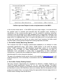
1.0
Introduction to the MS10 and MS1
The MS10 is a complete portable Audio Test Set that combines the functions
of an Oscillator (Signal Generator), Level Meter, Peak Programme Meter,
Noise Meter and Distortion Meter, along with Frequency, Phase, and tape
speed measurement, in one small hand-held unit that can be used on its own
or with a computer running the ‘Lin4Win’ support software (supplied free).
Its main feature though is ‘Sequence Testing’, introduced by Lindos twenty
years ago in the LA100 test set, and universally used by broadcasters and
studios for routine quality assurance ever since. It takes just two button
presses (SEQ followed by 3 for example) to run a typical test sequence that
can quantify any audio system in terms of levels, frequency response, phase,
distortion and noise in as little as twenty seconds, with results stored in the
unit. If a PC is connected, running Lin4Win, an impressive results sheet with
graphs and pass/fail tolerance testing appears immediately on the screen
ready to save, print, or even publish to the Web on our Test Sheet Database
for all to see! Because sequence tests carry (FSK) coded information they are
self-synchronising and fully automatic, even between any two MiniSonic units
on opposite sides of the world!
The emphasis throughout is on subjectively meaningful tests and one set of
quality standards, with only quasi-peak weighted (ITU-468) measurement of
both noise and distortion residue supported. This gives readings that are
pretty representative of what you will hear, whether you are testing a CD
player, an amplifier with crossover distortion (long considered impossible to
quantify - but we don’t agree), or a loudspeaker. With comparable
measurements, and a database fed by you, the user, we aim to challenge
much of the hype and make-believe that has taken over the audio world.
The MS1 is simply an MS10 with sequence reading disabled (except for a
sweep), sold at a price that is more affordable by schools and enthusiasts. As
sequence generation (which includes some LA100 compatible sequences) is
not disabled, it can also function as a low-cost generator for use with the
MS10 or LA100. The MS1 is easily upgraded to an MS10 by plugging in a new
firmware chip behind the removable ‘chiplid’ on the front panel.
1.1
Getting Started
Most users will not want to read through this manual, which is laid out as a
comprehensive reference guide, before getting started, so we suggest working
through the following brief tutorial as a quick way of becoming familiar with the
essentials.
1 Connect the Osc (output) and Input sockets together, using the Unison to
XLR leads provided, and Set the MIC/LINE toggle switch to LINE. If you are
4
using phono (RCA) or other ‘single-ended’ leads, note the automatic change
to consumer levels (see the UniSon section for full details).
2 Switch the unit on with the top right-hand toggle switch and check that the
display lights up. The unit will power-down (into ‘sleep’ mode) if no key is
pressed for 4 minutes: just press any key to restore operation.
3 Turn up the Volume with the slider control and you should hear a 1kHz
tone. Do not be disconcerted by the changing levels - the unit starts up in PPM
(Peak Programme Meter) mode and generates a line-up sequence to facilitate
use in certain fixed studio applications. Note how the changing L (left) channel
level is shown by a bright bar and the R channel level by a dimmer
‘shadowbar’. The speaker always monitors the L channel in level mode, but is
switched to the selected channel for Noise, Distortion etc.
4 Press LEVEL. This is the normal mode for measurements (faster response
than PPM mode). The output now goes to 1kHz at 0dBu on both channels and
both display bars merge reading 0dB on the bottom scale.
5 Hold FREQ down and press < or > to change the oscillator frequency. The
shadowbar now indicates the frequency being generated (top scale) and the
main bar shows the measured level on the L channel. Hold FINE instead and
th
the frequency changes in finer 1/12 octave steps. Hold dB and press < or >
to change the output level (1dB steps). Note that both these functions ‘wrap’ at
both ends to cover a huge range if desired. If this seems confusing, don’t
worry, as things are much more easily understood when you use a PC!
6 Press keys 3 & 4 together to reset and note how the battery voltage is
displayed if you hold them down (by the main bar – the ‘blurr’ shows the low
zone). There is currently no low-battery indication, so check battery voltage
from time to time. The oscillator output is now restored to 1kHz @ 0dBu.
7 Press Noise. The oscillator automatically mutes and the reading drops to
the lowest (‘under’) mark on the scale. Note that on the bottom scale 0db now
represents –50dB (L chan). If you were measuring a good 16-bit digital system
you might expect to see a reading of –16dB corresponding to –66dB (468-wtd
quasi-pk). You are measuring the noise level of the MS10 oscillator output
which is around –82dB and hence off the bottom off the scale (but not when
range changing is used). Press L or R to select either channel.
8 Press Dist. The unit will momentarily normalise the level, and then display
relative distortion (468 wtd quasi-pk). Again, the reading should be off the
bottom of the scale.
9 Press SEQ to enter sequence mode, and then press KEY1. This will run
sequence 1, which is a 5 second sweep. Note the audible FSK signal at the
start, which signals the start of the measurement and the segment type. Once
the sweep has finished you can use the < and > keys to move the cursor
(shadowbar) up and down the frequency scale and read off the stored levels
5
on the main bar. Holding SEQ and pressing R allows the R channel results to
be viewed. As you have a simple direct connection of course the levels will be
the same at all frequencies. Press LEV to leave sequence mode. This
completes a quick tour of manual stand-alone capabilities; now try out
operation with a computer:
10 Install Lin4Win on a PC (click on the CD drive and then double-click on
the ‘setup.exe’) and connect the Minisonic using the RS232 cable. Start
Lin4Win (from Start/All Programs menu). The control panel should open and a
status bar at the bottom left should show when connection has been
established. If the box keeps flashing red you may need to change the COM
PORT setting (menu options/coms setting). You are now ready to play with the
many features of the control panel which are largely self-evident.
11 Press SEQ on the unit followed by KEY3. This will run a 20-second
sequence of segments (n,u,r,q,z) and on completion you should see full
listings, with graphs, appear in the results window. Note that you can double
click on both the text and the graphs to bring up options and an expanded
graph with cursor readout. This demonstrates the full power of sequence
testing, which for many purposes may be all that you need to use. You can
now experiment with running other sequences, either from the keys, or by
entering any sequence of up to six segment letters (but note restrictions) in the
text box on the control panel under the RUN button. MiniSonic segments must
be entered as lower case letters as some LA100 segments also run on the
MS10. Press Return or click RUN to start the sequence.
Try out SEGh which produces an interesting (headroom) graph showing the
level at which a piece of equipment starts to limit or clip. To save results use
the shortcut CTRL-S. To open a saved file use CTRL-O. To print results use
CTRL-P. You will have to specify directories for saving in the usual way, and it
is a good idea to create a ‘Results’ directory first. Note that tolerances and
comments can be added.
You are now ready to test a piece of actual equipment. In some cases this will
require both the input and the output to be connected to the MS10. In others,
such as when testing a sound card output or a CD player, only the input of the
MS10 will be connected, the test signal coming from recordings of test
sequences or tones which are available as downloads from the
www.lindos.co.uk website.
What follows is a detailed reference guide to the various functions of the MS10
but you may find it more useful to skip to Section 4 for full details of Sequence
Testing, or Sections 9,10,11 which explain in detail how to test various specific
types of equipment.
6
2.0
Power On/Off and Basics
The unit is powered when the right-hand toggle switch is down. If no key is
pressed for 4-minutes it will automatically enter ‘sleep’ mode and the display
will go out. Press (don’t tap) any key to restore operation from sleep mode.
Battery life in sleep mode is over 5000hrs and both the working state and any
stored results are retained. Using the toggle switch to turn the unit on and off
will save battery life and ensure total reset, but any saved results will be lost.
To put the unit into sleep mode press keys 1 and 2 together. If any external
devices are taking power from the ‘UniSon’ input or output connectors this is
not turned off in sleep mode – toggle the power off to avoid a flat battery!
To disable automatic turn-off use startup option 1. The startup options (which
can be used together in combination) are:
Startup Option 1 – Power Lock (Hold Key1 while turning the power on)
disables auto-turn-off so the unit stays on until the battery runs down. The unit
also starts up muted – useful when testing speakers.
Startup Option 2 – Channel Ident (Hold Key2 while turning power on). This
changes the startup sequence from SEGj to SEGi (alternative line-up test).
Startup Option 3 – Glits Tones (Hold Key3 while turning power on). This
alters the start-up sequence to GLITS (as used by the BBC).
Startup Option 4 – Direct Trigger (Hold Key4 while turning power on)
enables Direct Trigger in sequence mode, meaning that segment characters
are passed internally from generator to measuring set, rather than by FSK
(frequency shift keyed) signalling over the measurement path. This is useful
for testing devices that attenuate frequencies in the 1650 to 1850Hz region
used by the FSK, such as sub-woofers, and crossover-filters. Sequence
measurement commences when a key is pressed to send the sequence or
segment, even if no signal path exists.
Startup Option 9 – LA100 Sequence Generation (Hold SEQ while turning
the power on). This selects LA100-compatible sequence generation in
sequence mode for inter-working with the earlier Lindos LA100 test set. See
section 4.5 for full details of the LA100 sequences available. Recognition of
LA100 segments works without setting this option, though only to a limited
extent in this firmware version (M3.0).
2.1
Reset
Pressing KEY3 and KEY4 together resets the unit to start-up conditions. The
display flashes momentarily into battery test, the oscillator resets to 0dB and
1kHz output, and Level mode is set. The sequence data and results listing are
cleared, but power-lock is not cleared. Pressing LEVEL performs a lower level
of reset, cancelling relative reading, range settings, level options and vernier
mode and selecting both channels, so when you press LEVEL you can be
7
sure that you are simply reading levels, though oscillator settings and
sequence results are not reset. Pressing any of the function keys – Level,
Noise, Dist, Seq, PPM, cancels any options or range settings, ensuring a
consistent basic reading for ease of stand-alone use.
2.2
Monitor Volume
The speaker enables the measured signal to be heard at a loudness level set
by a small slider VOL control on top of the case. Only the left internal channel
is monitored in Level or PPM modes, but plugging in headphones disables the
speaker and allows high-quality listening in stereo. In other modes the speaker
monitors the selected channel and is often useful because it enables the
nature of noise or distortion residues, or the progress of a sequence test to be
heard.
2.3
The ‘Line-Up’ Sequence
A special, repeating, ‘line-up and channel-ident’ sequence is generated at
power switch-on (to allow fixed use as a line-up generator in broadcast
applications). Line-up sequences are often recorded at the start of programme
material as confirmation of alignment level and channel assignment for
broadcasting. Currently SEGj is used, which increases the level to +8dB on
the L channel first, then on both channels. It combines the ability to identify L
and R channels heard together or in isolation, with a check of max level
(PPM6 is +8dB), but this can be easily changed on request to the ‘GLITS’ or
other tests (contact Lindos for special firmware chip). To stop the line-up
sequence press LEV (or NOISE or DIST) and normal oscillator operation will
take over.
2.4
Battery / External Powering and Charging
Hold down keys 3 and 4 together to read the battery voltage. On a fully
charged battery (8.3V) the main bar should be at maximum (RH red LED lit),
and as the voltage drops the indication will fall until it enters the patterned ‘no
go’ zone at about 6V. The unit will cut out suddenly at around 5.5V, and at
present no other battery-low warning is given. Over 16 hrs of use should be
possible on the 1.85 A-hr battery supplied.
The MiniSonic may be powered externally using the 12V mains adapter
supplied by us (100 to 240V supply) or any other power supply, preferably of
the regulated type. The power connector is 1.6mm centre positive and
protected against reverse polarity. Powering from a car battery is also
permissible, the internal regulator taking care of voltages up to 14. Current
consumption is only 100mA, but rises to 300mA when charging a flat battery.
The Lithium Ion battery charges whenever external power is connected, the
charge rate reducing to zero as full charge is approached so that continuous
use on external power will not degrade battery life at all. External fast-charging
in one of the many available camcorder battery chargers is also possible, as is
8
the use of the bigger capacity batteries that are available with compatible
(Sony) fitting (versions with or without ‘Info-Lithium’ are suitable).
Note that the unit will turn on as soon as external power is applied, even with
the toggle set to off, (to facilitate use in fixed installations as a PPM, alignment
tone generator etc), with auto-turn-off automatically inhibited. Since the latter
is achieved by sensing whether the voltage is sufficient to light the top red
indicator on the battery test (around 8.1V), auto-turn-off is also disabled on a
well-charged battery. Switching the toggle to ON provides battery backup in
the event of brief power failure. Lithium Ion batteries normally retain charge for
at least a year, even when they are several years old (expected life is over ten
years), and are internally protected against over-discharge etc. Operation from
a PP3 Alkaline battery is possible (5hrs intermittent use) (request adapter lead
from Lindos or use a diode in series to prevent explosion through charging!) A
PowerBus for external microphone preamps and other devices is provided on
pin 5 of all input and output (UniSon) sockets. This is at 6 - 8V, (for regulation
to 5V in the device) current limited at 1 - 1.5A for safety (sometimes this pin
may be accidentally grounded by contact with the connector shell as it is
inserted, in which case the unit will be seen to reset due to brief loss of
power). Powering the MS10 via the UniSon PowerBus, without a battery, is
also possible.
3.0 Stand-Alone Use (No computer
connected)
Connect the Osc (output) and Input sockets to the unit to be tested using the
leads supplied as appropriate: Unison to XLR for professional equipment or
Unison to Phono for consumer equipment. Other leads such as Unison to
3.5mm Minijack (for computers and portable devices), or Unison to Jack
(small tip for broadcast or large tip for guitar amps etc) are available from
Lindos.
ENSURE THAT THE MIC/LINE TOGGLE IS SET TO LINE (unless
microphone operation is required, or results will read 6dB low!).
3.1
Level Measurement
Press LEVEL. The range is fixed (0dB) and covers -20 to +10dB relative to
alignment level, which corresponds to 0dBu (0.775V rms) with balanced leads
(XLR), but -6dBu (Lindos Unison standard) when unbalanced (phono or minijack) leads are used. Both channels are displayed - the bright bar indicates the
L channel, while the ‘shadowbar’ shows the R channel - but just one may be
selected using the L or R buttons. Pressing LEVEL (or L and R together)
restores both channels. Although levels are only indicated to the nearest 1dB
they can easily be read to 0.05dB resolution (indicated on the shadowbar)
using the novel ‘Vernier’ facility (see section 5.1). Normalising and range
9
changing are also possible (see 5.3 and 5.4). Level measurements use a
rectifier with fast Quasi-Peak characteristics, not true rms (root mean square).
For most measurements, on sine wave signals, this is of no consequence, and
the readings correspond to rms value. The term Quasi-Peak refers to any
rectifier (detector) that responds essentially to the peak of the signal, but takes
a significant time to respond (integration time). Increasing the input to a digital
system beyond the clipping limit would continue to produce an increasing
output reading on a true-rms rectifier, as the waveform became flattened, but
a Quasi-Peak reading ceases to rise abruptly at the rms sine-wave equivalent
of the clipping level. This is a very useful feature, made use of in the special
headroom test segment (SEGh).
Level Option 1 – Phase (press LEV and key1 together). This selects phase
display on the unit (see section 3.6).
Level Option 2 – Ultra-Fast Level (press LEV and key2 together). This
selects level measurement with a very fast response; reducing attack and
decay times by a factor of ten, which may prove useful when making rapid
adjustments.
Level Option 3 – Frequency (press LEV and key3 together). This selects
frequency display on the unit (see section 3.5).
Level Option 4 – Vernier Mode (press LEV and key4 together). This selects
‘vernier’ mode for high resolution (see section 5.1).
3.2
Noise Measurement
Press NOISE. The range is fixed (-50dB, meaning that 0 on the bottom scale
corresponds to –50dBu), and so covers -70 to -40dBu. Readings are of
absolute level, unless the REL indicator is flashing. To read noise relative to
the test level, press DIST, wait a second, and then press NOISE. This is just a
convenient way to save the ‘Test Level’, which is the reading for the current
oscillator setting, as a Reference Level; a process called Normalising (see 5.3
for more details). Only the left channel is displayed, (the MS10 includes only
one set of measurement filters) but pressing R selects the other channel.
Pressing NOISE (or L) restores L channel operation. The oscillator output is
automatically muted (though it can be de-muted) and measurements are
ITU-468 Weighted (formerly CCIR468-4 plus IEC and BS standards), with the
exception that the Quasi-Peak response has been given a faster decay time
for quick settling (tone-burst response times are still to 468 specification). The
NOISE key may be held down for a true 468 decay time, though this will
normally make no difference unless successive impulsive noises - clicks and
pops - occur within a few seconds of each other; a situation that used to
concern engineers working with telephone links and is now something to
watch for on computer sound card outputs. The use of a faster decay time,
together with a brief initial fast-settling period (also invoked on range-changes
when used with a PC), makes 468 Quasi-Peak measurement much more
10
user-friendly. Where other instruments may take many seconds to settle to a
stable reading, the MS10 is so fast that it is even possible to take readings
during brief pauses in actual programme material.
Noise is often expressed as ‘Signal to Noise Ratio’ or ‘Dynamic Range’, but
these terms are confusing, as they do not refer to any standard method. There
is no such thing as ‘signal level’ on music or speech except from moment to
moment! Dynamic range is often taken to mean the difference between max
signal level and noise level, but it is also used to refer to the difference
between max signal level (full scale digital) and muted noise level (without
dither and hence just analog output noise) on CD players. This is too
confusing, especially since many CD players use output muting in the
absence of signal to achieve an even lower level.
What really matters is how far the noise is below a typical signal, and though
there is really no such thing as a typical signal level, it is a good idea to
establish a nominal one, call it ‘alignment level’ (AL) and measure noise
relative to this. All broadcast measurements are made relative to ‘alignment
level’, which usually corresponds to 0dBu (0.775Vrms) on all analog paths.
Maximum permitted level, or full-scale digital (FS), will be above this by an
amount referred to as ‘Headroom’, usually 18dB (EBU recommendation) on
digital recordings, or 24dB on some original material. Headroom is typically
12dB or less on broadcast paths, where the EBU recommends +9dB max
level when measured on a PPM (which does not read the true peaks).
The great merit of this system is that a noise measurement made relative to
Alignment Level will always be a reasonable guide to the true intrusiveness of
the noise onto typical material, regardless of the headroom. Where less
headroom is available for transmission, compression or limiting will usually be
used to reduce brief peaks, but this has little effect on overall perceived
loudness. A recording may start life with 24dB of headroom, and end up with
only 9dB of headroom at the listener’s radio or television. Its ‘dynamic range’
has indeed been reduced, but it will not sound any noisier, assuming that it is
the peaks that have been limited. Instead it will have lost ‘sparkle’ and impact.
Specifying noise and headroom separately reflects these different qualities
properly.
Noise Option 2 – Crosstalk (press NOISE and key 2 together). This selects
Crosstalk measurement (see section 3.4).
Noise Option 3 – True ITU-468 Q-pk (press NOISE and key 3 together).
This selects the correct (slower) decay on the quasi-pk rectifier.
3.3
Distortion Residue Measurement
Press DIST. The oscillator will generate 1kHz and the unit will very briefly
measure the level of the incoming tone, saving it as a reference level and then
switching to relative-level mode as shown by the dBu/Rel indicator flashing.
11
This is also called ‘normalising’. The distortion-residue level is then indicated
on a fixed range (-40dB) (corresponding to 0 on the bottom scale), which
therefore allows readings of -60 to -30dB to be made. Only the left channel is
displayed, unless R is pressed. Pressing DIST or L restores left channel
operation. The oscillator output is automatically set to 1kHz, but any level may
be set as required. What is measured is the relative level of all harmonics and
noise in the frequency range 2kHz to 20kHz, using 468-weighting and
quasi-peak response (a method strongly favoured by Lindos and also
incorporated into the IEC-268 standard). The dBu/REL button toggles relative
measurement on and off, allowing the absolute level of distortion-residue to be
read if desired. The detailed merits of weighted distortion-residue
measurement are discussed in later sections, but essentially the method takes
proper account of the high order harmonics caused by crossover distortion or
digital quantising errors, and also gives due emphasis to the high frequency
modulation noise that can cause a characteristic ‘roughness’ on tape or
compact cassette. Distortion-residue readings will generally be higher than if
they were measured using the commonly quoted THD (total harmonic
distortion rms) method, and on harsh crossover-distortion they may be 15 or
20 dB higher. Furthermore, readings may be much higher than those
commonly quoted in equipment specifications because the latter often refer to
measurement at maximum output level or full scale digital level, a practice that
is to be condemned as it gives high figures but does not reveal what really
matters. A typical DIST measurement on a 16-bit system might read –20
(representing –60dB) but compact cassette will read +5 (-35dB) or higher, so
the fixed scale has been chosen to encompass this large variation. Use rangechanging (section 5.4) if the reading is off the scale. To measure relative
distortion residue at levels other than 0dB, just set the required oscillator
output level before pressing DIST.
3.4
Crosstalk Measurement (NOISE option 2)
Press NOISE and 2 together (two LEDS will light up). Operation is exactly as
for noise, with the same 468-Weighting and Q-Pk response, but one channel
of the oscillator output is always muted while the other is driven at the set level
and frequency, which may be adjusted while reading crosstalk. Measurements
are of absolute level, unless a reference level has been saved by ‘normalising’
(or previously pressing DIST which normalises), in which case the REL
indicator will be flashing.
Crosstalk can be measured at any frequency or level, simply by changing the
oscillator settings, but note that the measurement is 468-Weighted, which
greatly emphasises readings around 6.3kHz (by 12.2dB). Use of the automatic
sequence test for crosstalk (SEGc) is recommended as this automatically
changes the test level to give results that comply with a standard originally
devised by the IBA (Independent Broadcasting Authority (UK) now disbanded)
for broadcast testing, with regard to both the (milder) IBA-recommended
12
weighting curve and the maximum permitted levels that apply where 50us preemphasis is in use (such as on FM transmitters).
3.5
Frequency Measurement (LEV option 3)
Press LEVEL and key 3 together. The LEVEL indicator will flash to remind you
that the ‘shadowbar’ (which appears feinter) now indicates frequency (to the
nearest third octave) on the top scale. The level is displayed simultaneously
by the main bar, for the L channel only, unless R has been pressed to select
the other channel. Though not very precise, the frequency readout is graphic
and fast: very useful for identifying frequency bands on test tapes or disks.
Precise frequency measurement is available when using Lin4WinXP on a PC.
Note that frequency is only read on the left channel.
3.6
Phase Measurement (LEV option 1)
Press LEVEL and key 1 together. The LEVEL and DIST indicators will flash to
indicate that PHASE measurement is selected. The main bar will indicate the
level on the selected channel while the ‘shadowbar’ will indicate the phase
difference between the channels on a scale centred around the 0dB mark with
20 degrees per division. Thus 0 indicates zero phase difference, and +1
indicates +20 degrees, while +9 corresponds to the maximum of +180
degrees, and –9 to the minimum of –180 degrees. Phase measurement works
up to 40kHz and down to about 40Hz. Note that the left channel is considered
the reference so that a +ve reading indicates that R channel leads the left and
a –ve reading means that the R channel lags behind the left. This was chosen
because the L channel is used for FSK signalling on sequences and so is the
preferred channel to use as a directly connected reference when measuring
absolute phase in-out on a piece of equipment. Phase difference between
channels causes shifting of the stereo image, and is a useful measurement to
make when checking the azimuth alignment of heads on analog tape
machines. There are circumstances though in which the phase delay in a
single channel is of interest, for example when attempting to ‘time align’
separate drivers in a wide range loudspeaker. In this case, the left channel
input and output of the MiniSonic should be connected directly and treated as
the reference signal (by plugging the XLR’s together or by making up a special
lead incorporating the link. The R channel input is then connected to the
output of the device under test (crossover network etc) so that what is
displayed becomes the input-to-output phase shift.
For microphone measurements a special trick can be used taking advantage
of the fact that when MIC is selected on the MiniSonic, the –ve UniSon inputs
remain functional and any input to them is summed with the Microphone
signal. A single wire connection between the –ve output and –ve input of the
left channel can therefore be used to provide a reference signal, allowing
absolute phase to be measured using a microphone plugged into the right mic
input. Do not attempt to use the standard XLR input lead to achieve this
13
(capacitive coupling in the lead to the floating +ve input will cause problems).
A D-type plug with a single wire to pin 1 (from pin 1 on the output connector) is
required (or Lindos can supply a special lead-set). Using such a set-up, the
microphone will show phase at a given distance from a speaker. Alternatively
it is possible to use two microphones and simply observe the phase difference
between them. This can be useful for checking the time alignment of a subwoofer for example, with one mic placed by the sub-woofer and the other by
the main speaker.
3.7
PPM (Peak Programme Meter) Use
Press PPM. Both channels are displayed with accurate IEC (type Ilb ie
UK/BBC – British Broadcasting Corporation) dynamics, so this mode is ideal
for checking the legality of programme levels for broadcast or recording. The
range is set to 0dB on pressing PPM for use with standard broadcast levels,
but the input gain may be adjusted by holding down the PPM key and using
the up-down (L-R) keys. While PPM is held, the ‘shadowbar’ displays the gain
setting. Note that it ‘wraps’ at top and bottom allowing gain settings from -50 to
+30dB; if you step up the gain, for example, beyond +9 the shadowbar will
jump to –20, and then continue up to 0 corresponding to +30dB gain. The
LINE OUT UniSon socket provides a gain-controlled output for recording
purposes, with alignment level 0dBu out at PPM4 (0dB on the scale).
Selecting MIC on the toggle turns this mode into a microphone recording setup for voice-overs, location recording etc. Note that +8dB corresponds to
PPM6 or maximum permitted level for broadcast material (EBU absolute max
is +9dB), while 0dB is PPM4 or ‘normal’ level. A self-adhesive label with clear
standard PPM markings (1 to 7) can be supplied by Lindos for sticking on top
of the frequency scale, if this is preferred. A scale centred conventionally on
PPM4 is also possible (consult Lindos for special firmware chip).
PPM Option 2 – Fast attack PPM (press PPM and key 2 together) provides
an alternative PPM with very fast attack (integration time of under 1ms) on
both channels. Decay time is as standard.
PPM Option 3 – Dual Speed PPM (press PPM and key 3 together) selects a
dual-attack PPM operating from the L channel only. The main bar retains
standard PPM characteristics while the ‘shadowbar’ has the very fast attack of
option 2. This will be found useful for detecting whether brief peaks have been
compressed. On uncompressed live percussive sounds a difference of 5 to
15dB will be observed between the two readings, as can be demonstrated by
simply plugging a Lindos miniature microphone into the left MIC socket,
selecting MIC, and banging two spoons together! This test demonstrates
convincingly why recording with realism requires 18dB or more of headroom
for the brief loud peaks that have little effect on perceived loudness (the ear
has a reduced response to brief bursts), yet are vital to maintain ‘sparkle’ on
percussive sounds. Using this mode to check recordings will reveal the extent
to which brief peaks have been limited or compressed. Unfortunately, on
14
broadcasts and a great many recent CD’s the two bars will rarely be seen to
separate by more than 1 or 2dB!
PPM Option 4 – Tape Speed and Flutter (press PPM and key4 together)
selects speed and flutter measurement (see below).
3.8
Tape Speed and Flutter (PPM option 4)
Press PPM and key 4 together to select this mode. The PPM and DIST LED’s
should light up. The shadowbar indicates deviation in speed (on a 3.15kHz
tone) with readings centred on the 0dB mark and sensitivity of 0.2% per
division (+2% to -4% scale range). Outside this range a ‘rolling’ pattern may
appear.
Tape flutter (not currently implemented – later upgrade?), (also known as
‘Wow and Flutter’ is measured weighted quasi-pk to IEC386 and indicated by
the main bar in dB, with 0dB representing 0.1%, so that +10dB represents
0.3% and –10dB 0.03%. While wow and flutter used to be treated separately,
with wow referring to slow speed variations below about 1Hz and flutter to the
faster variations, the use of the weighting curve now allows a single
meaningful measurement. The curve peaks at 4Hz (the most annoying
variation) rolling off at higher and lower frequencies.
3.9
Oscillator Use
Setting The Output Frequency
Oscillator setting is best demonstrated in LEVEL mode, though it works in
other modes. Hold FREQ while operating the up-down (L-R) keys to change
the frequency in 1/3-Octave steps. The ‘shadowbar’ will temporarily become a
cursor indicating the selected frequency (top scale), while the main bar
continues to read the L channel input level normally. Hold FINE, instead of
FREQ, to change the frequency in 1/12-octave steps. Note that the cursor
‘wraps’ at both ends in such a way as to allow frequencies down to 4Hz and
up to 40kHz to be set. Just above 40kHz will be found 1kHz, 5kHz, and 10kHz
square waves and just below 4Hz is generator mute. At reset or switch-on the
oscillator is set to 1kHz at 0dB.
Setting the Output Level
Hold dB while operating the up-down keys to change the level in 1dB steps,
again indicated by the ‘shadowbar’ acting as a cursor. Again, the cursor
‘wraps’ at both ends, allowing levels between -90 and +19dBu to be set. If this
confuses, just reset and try again.
Channel Selection and Mute
Press MUTE to silence the output. Press again to restore both channels (or
press dB). Hold MUTE and press L (or R) to output on the L (or R) channel
only (may need two attempts – only works after muting).
15
4.0
Sequence Testing
Lindos Sequence Testing is a powerful innovation, first incorporated into the
LA100 in 1984 and universally used by broadcasters worldwide ever since. A
MiniSonic Sequence consists of up to six segments; where segments are like
building blocks that can be chosen by the user. Each segment generates a
particular sequence of tones, a sweep, or silence, intended to test a particular
parameter, such as frequency response, distortion or noise. It begins by
sending its identifying character, (in ASCII code) as a frequency-shift-keyed
(FSK 110-baud) signal which acts as a synchronising trigger as well as the
instruction for a series of timed measurements. This means of course that the
responding MiniSonic does not have to be the one generating the sequence; it
doesn’t even have to be on the same side of the world but may be at the other
end of a satellite link or line.
Because the measuring side of a MiniSonic unit operates quite independently
from the generating side, the signal may be delayed; by a fraction of a second,
as is the case when testing two-head tape machines, or by years, as when
playing back a tape that has had a sequence test recorded on it for future
quality checking. Any MiniSonic unit in SEQ mode will respond instantly to an
appropriate FSK signal at its input, and go into the appropriate series of
measurements for the specified segment. At the end of each segment it waits
for up to one second for the next segment, and when no more segments are
detected it times out with the results saved in its memory for viewing or
printing. If a PC running Lin4Win is connected, the results will appear on the
screen about a second after the sequence has finished running, in the form of
a Results Sheet that can be saved or printed as an A4 page. Sequence 1 for
th
example, will produce a 1/6 -octave plot of frequency response, for two
channels, in just five seconds. Sequence 3 will produce a complete set of
results, with graphs and bar charts, of frequency response, relative phase, test
levels, noise, and distortion at six levels, in just 20 seconds. Many other
variations are possible by combining segments, especially when using the
Lin4Win support software running on a PC (see section 10).
4.1
Inter-working with the LA100
The MS10 normally uses segments that are different from those recognised
by the LA100, because its design made a faster and better set possible.
MiniSonic segments take advantage of the MS10’s ability to measure levels
on both channels simultaneously as well as its ‘smart-rectifier’ which changes
speed for fast settling on all measurements. The Dist Residue segments (q
and r) in particular provide a powerful test of weighted distortion at six levels,
which is not practicable on the LA100 because of settling limitations.
To distinguish them from LA100 segments, MiniSonic segments are
characterised by lower-case characters (the LA100 uses mostly capitals).
They are only sent once, both channels being measured simultaneously on
16
sweeps, or in rapid succession during other segments (the LA100 sends each
segment twice, once for each channel). Segments only start with a single FSK
character (the LA100 generally uses two, the first being a channel specifier).
Where the LA100 uses a ‘stop’ character to mark the end of a sequence, the
MiniSonic simply waits one second after it has finished logging each segment,
and times out (bringing up results) if further FSK is not detected in this time.
These innovations make for much faster testing.
Recognising that it might nevertheless be useful to use the MS10 in an LA100
environment (especially on lines and links), a degree of compatibility has now
been achieved, by providing for generation of the most commonly used LA100
segments. Lin4Win now distinguishes the appropriate upper-case letters
entered in the run box from normal lower-case MiniSonic segments, enabling
a variety of LA100 sequences to be set up (enter each letter only once – it will
automatically run twice where appropriate). For stand-alone use the MS10 can
be put into ‘LA100 mode’ using startup option 9 (hold SEQ and turn on the
power). Keys 1 to 4 then run four popular LA100 sequences, rather than
MiniSonic sequences, when in SEQ mode (see sections 4.4 and 4.5 for
listings), making the MS10 a useful partner to the LA102 measuring set for
network testing. The recognition and logging of a few LA100 segments has
also been added (SEGS T,V,U,R,N) but further work is needed for these to
work reliably in actual LA100 generated sequences (currently the MS10 will
time out on segments it cannot recognise, and is confused by some of the
sequences or text headers normally sent by the LA101).
4.2
Running a Sequence
Press SEQ to put the unit into sequence read mode. The bar display now
indicates the contents of the memory from the last frequency response sweep
that was run (or nothing). To run a sequence simply press one of the number
keys 1 to 4 (see below for SEQ 5 to 13). A sequence of test Segments is
generated, and assuming that a path exists to the input of the MS10 this will
be responded to. If a PC running Lin4Win is connected, then completion of the
sequence is indicated by the appearance of a results page on the screen.
Alternatively, it may be of interest to follow the progress of a sequence by
turning up the volume control and listening, or by watching the MiniSonic bar
display. The ‘shadowbar’ acts as a progress indicator, moving from left to right
for each segment, while the main bar indicates the instantaneous value of the
measurement. The SEQ indicator flashes while a sequence is being
generated, and stops when sequence generation ends. The REL indicator
flashes if master-seg m or n is responded to, to indicate that relative reading is
in progress. Note that the FSK trigger is only recognised on the left channel,
and that it requires a path that can transmit signals around 1.8 kHz. Use ‘direct
trigger’ (startup option 4) to test low-frequency-only paths, such as subwoofers or crossover filters. FSK operation means of course that another
MiniSonic may be used for measurement, even at the distant end of a line or
17
satellite link. Loudspeaker measurements can also be made conveniently.
In-car speaker responses may be measured, for example, by playing a sweep
segment from a test tape or CD (available from Lindos, or as a download),
with automatic triggering from the microphone signal so that no electrical
connection is required. Computer Sound-Cards and MP3 players can be
tested using downloaded test sequence files (available at www.lindos.co.uk).
All sequence levels are generated relative to the basic oscillator level set prior
to running them (0dBu unless altered). To ensure that this is 0dB, if in doubt,
just do a reset (keys 3 and 4) prior to entering sequence mode. In some
instances, of course, it will be desirable to run a sequence at a chosen level,
for example when testing low-level microphone inputs.
4.3
Choosing Sequences and Segments
Sequences 1 to 4 are ordered according to complexity (and time taken). SEQ3
is probably the most useful, as it tests most things in 20 secs, but because it
tests distortion with tones up to +18dB AL it is not suitable for broadcast tests.
SEQ2, which only tests up to +8dB AL, is suited to digital broadcast tests, but
SEQ6, which uses less sensitive measurement ranges on noise and
distortion, and also runs the sweep at –10dB is better suited to FM transmitter
paths where pre-emphasis would cause overload at high frequencies on a
0dB sweep. SEQ4 is SEQ3 plus a 20 second noise plot, providing a more
thorough test of computers and devices that might have occasional noise
clicks. It is useful to remember that these basic sequences can be modified by
the subsequent running of certain segments, in particular SEGs (slow
sweep)(press SEQ+key1) for more detailed results on speakers in reverberant
surroundings, SEGw (wide sweep)(press SEQ+key5) for testing 96k digital
system bandwidth, or SEGc (crosstalk) (press SEQ+REL). These are
available in stand-alone use, by using the key combinations shown above,
and because a master-seg is not run again they replace or add to the
segments already run. Where the initial sequence incorporated a normalising
master-seg, the added segments are also normalised. Running a master-seg
(or resetting) clears existing results.
18
Notes on Sequences and Segment Limitations
Any combination of segments (up to 6) can be sent as a sequence using the
Lin4Win support software running on a PC, with the following provisos:
Only one ‘Master-seg’ can be sent (usually n) (or m or t)
Only one Sweep seg can be sent (usually u) (or s, or v, or w, or h)
Only one extra plot can be viewed (l or z)
SEGz only works with a sweep (it signals the showing of phase)
SEGt used in place of SEGm adds (azimuth) alignment tones
SEGq runs SEGr too (they share a common text header in results)
Attempting to run LA100 segments alone will usually result in other segments
being run automatically. This is because the LA100 requires message text at
the beginning and a terminating character at the end. SegT incorporates the
header text and also normalises. SegZ (phase) incorporates the terminating
character.
Segment letters can be entered in any order, either in the control panel or at
the top of the main (results) window (press return to send) – the sending order
is fixed (eg nurqcl)
SEGq actually tests distortion at +11.5, +14.5, and +17.5dB rather than the
nominal +12, +15 and +18dB quoted for simplicity. This provides a margin of
safety to avoid ‘just clipping’ when equipment is not precisely aligned.
4.4
Viewing Sweep Results on the Unit
Whilst the only way to view a complete set of sequence results is on a
personal computer using the Lin4WinXP program, it is possible to examine a
frequency response plot on the MiniSonic in a novel way. Simply use the
up-down (L-R) keys, with the unit in sequence mode, to move the cursor
(‘shadowbar’) up and down the frequency scale as marked above the LED
display. The main bar will indicate the level stored for each frequency. Though
simple, this form of display is still very useful, especially when measuring
speakers, because sweep results triggered automatically from the microphone
signal, and captured in just five-seconds, can be studied at leisure and in
silence. Normally the L channel is displayed. Hold SEQ and press R to select
right channel display. Press SEQ (or SEQ-L) to return to the left channel.
19
4.5
Standard Sequences (v3.0 firmware chip)
MS1 Units run all sequences, but only respond to SEGu (sweep)
Description:
Segs:
Measures:
SEQ0
Line-Up
j
0dB/+8dB line-up/chan ident
SEQ1
‘Sweep’
u
sweep 20Hz-20kHz 5 secs
SEQ2
‘Broadcast Test’
n,u,r,z
sweep, phase, noise, dist to +8dB
SEQ3
‘Digital Test’
n,u,r,q,z
sweep, phase noise, dist to +18dB
SEQ4
‘Sound-card Test’
n,u,r,q,l
digital test plus 20s noise plot
SEQ5
‘Slow Sweep’
s
sweep 20Hz-20kHz 20 secs
SEQ6
‘Tape/FM Test’
m,v,r,z
sweep @ -10dB, & high ranges
SEQ7
‘GLITS Test’
g
channel ident and line-up
SEQ8
‘Wideband Sweep’
w
sweep 40Hz-40kHz 5 secs
SEQ9
‘Headroom plot’
h
level versus level 0dB to +18
SEQ10
‘Long Noise plot’
l
noise peak and mean 20 secs
SEQ11
‘Distortion segs
r,q
distortion residue –20 to +18dB
SEQ12
‘PPM tone bursts’
p
5 ‘inverse-level’ tone-bursts
SEQ13
‘Crosstalk’
c
crosstalk at 100Hz 3.15k 10kHz
SEQ1
‘Sweep, Phase, TL’
TUY
SEQ2
‘General’
TRINY
sweep @-10 phase, noise, dist
SEQ3
‘Digital Test’
TUDNY
sweep @ 0dB, phase noise, dist
SEQ4
‘Broadcast Test’
VRAGNY
sweep etc with 50us de-emphasis
Special LA100 Sequences: (startup option 9)
sweep 20Hz-20kHz 5 secs
Notes:
SEQ0 only runs at initial switch-on (until a function key is pressed)
To run SEQ5 hold the SEQ key down while pressing key 1
To run SEQ6 hold the SEQ key down while pressing key 2 (etc to SEQ 8)
To run SEQ9 hold the SEQ key down while pressing LEV
To run SEQ10, 11, 12, 13, hold the SEQ key down while pressing NOISE, DIST, PPM, REL
To run LA100 sequences, hold down SEQ while turning on the power.
Any Sequence of segments can be sent using Lin4Win, but see limitations in section 4.3.
20
4.6
Segments Available (v3.0 firmware)
Name:
Description:
Details:
SEG n
Master-seg
Test lev/Normalise 1kHz /Noise (-85 to –50dB)/Delay
Sequence building segments
SEG m
Tape/FM Master-seg Test lev/Normalise 400Hz/Noise (-60 to –30dB)/Delay/Speed
SEG t
Test-Tape Intro
3.150kHz 8s,10kHz 8s,1kHz 8s, then as SEGm (azimuth)
SEG u
Sweep
20Hz – 20kHz @ 0dB 5 secs
SEG v
Tape Sweep
20Hz – 20kHz @ -10dB 5 secs
SEG w
Wide Sweep
40Hz – 40kHz @ 0dB 5 secs
SEG s
Slow Sweep
20Hz – 20kHz @ 0dB 20 secs
SEG r
Distortion Residue
Dist Res 1kHz @ -20, 0, +8dB
SEG q
Dist Res to +18
Dist Res 1kHz @ 0, +12, +18dB
SEG c
Crosstalk
Crosstalk at 100Hz, 3.15kHz, 10kHz @ 0dB IBA-wtd
SEG h
Headroom Plot
1kHz 0dB to +18dB in 1dB steps 5 sec plot
SEG l
Long Noise Plot
Noise Wtd 468 (-85 to –50dB) L-chan 20 sec plot
SEG p
PPM Tone-burst test
Details:
Special Purpose Segments:
‘Inverse Tone Bursts’ 1, 1.5, 5, 10, 100ms
SEG y
468-Wtd Tone-bursts ‘Inverse Tone Bursts’ 1, 1.5, 5, 10, 100ms
SEG b
Tone-bursts
General Tone Bursts 100, 10, 5, 1, 0.5ms @ 0dB
Flutter-meter cal wobble (should read 1.1% IEC Wtd)
SEG e
Flutter Cal Wobble
SEG f
Flutter Test
3.15kHz 20 sec (provisional - not yet recognised)
SEG i
Channel Ident
1kHz 0dB 1 sec, 1kHz –6dB 1 sec, repeating
SEG j
Lindos Lineup
1kHz 0dB L+R 2secs, +8 dB L 2s, +8 L+R 2s repeating
SEG g
‘GLITS’ test
1kHz –3dB 6s total 1 mute on L , 2 mutes R repeating
SEG z
Phase (FSK only)
Phase Plot (valid only above 1kHz) (Use with u,v,s, or w)
SEG/
Sequence Separator
Use in Lin4Win to separate multiple-sequence generation
SEG<
Repeat (<n optional)
Use in Lin4Win to repeat indefinitely (<3 does 3 repeats)
LA100 Segments:
(* = not currently logged by the MS10)
SEGT
Test Level 1kHz
1kHz @ 0dB (includes ‘MS10’ start text) 1 sec
SEGV
Test Level 400Hz
400Hz @ 0dB (includes ‘MS10’ start text) 1 sec
SEGU
Sweep
20Hz – 20kHz @ 0dB 5 secs
SEGR
Tape Sweep
20Hz – 20kHz @ -10dB 5 secs
SEGD*
Distortion (THD)
100Hz, 1kHz, 6.3kHz @ +8dB 6 secs
SEGG*
Distortion 50us
40, 100, 315, 1k, 6k3, 10kHz with 50us de-emphasis 18 secs
SEGI*
Distortion (THD)
100, 1kHz @ +8 and –10dB 8 secs
SEGA*
Crosstalk
40, 100, 315, 1k, 6k3, 10kHz with 50us de-emphasis 6 secs
SEGN
Noise
mute for 8 secs
SEGW*
Wow & Flutter
3.150kHz for 12 secs
SEGY
Phase (and stop)
40, 100, 1k, 6k3, 10k, 15k (includes stop and seg count)
21
5.0
5.1
Advanced Features
Vernier Precision
Pressing KEY4 and LEVEL together selects VERNIER mode enabling levels
to be measured to much higher resolution than the 1dB steps possible with
the normal LED display. Only the L channel is displayed (unless R is pressed)
and the ‘shadowbar’ now indicates the fractional reading from +0.5dB to
-0.5dB by which the integer reading is in error. The shadowbar is centred at 0
on the bottom scale and can move between -10 (-0.5dB) and +10 (+0.5db) in
0.05dB increments. To adjust a level to 0dB, for example, simply aim for both
bars being on zero. Given an input level of, for example, +2.25dB, the main
bar will read +2 and the shadowbar +5. Turning up a level gradually will cause
the vernier to move smoothly up to +10 and then jump down to -10 repeating
for every 1dB of increase. Looking at the MiniSonic’s own output in vernier
mode, at varying levels, will simply indicate the unit’s total fractional dB error
for every 1dB step. The vernier indication may become ‘noisy’ on levels below
-6dB. The vernier facility is only available in LEVEL mode: to cancel it just
press LEVEL (or any other function key).
5.2
Relative Levels
A REFERENCE level is stored in the unit at all times, and this is set to 0dB at
switch-on. Pressing dBu/REL makes all readings read relative to the reference
level, and pressing it again returns to absolute reading. The red LED above
the button flashes when relative readings are being made.
5.3
Normalising
Holding down the dBu/REL key for at least one second, while in LEVEL mode
stores the current input level as the Reference Level (and toggles to relative
reading as shown by the flashing indicator). The reading should therefore
jump to 0dB: if it doesn’t (as occasionally happens for big changes), just press
and hold again. All subsequent readings, in all modes, may be made either
absolute or relative to this stored level simply by toggling dBu/REL on or off.
This is most useful for relative noise readings at non-standard alignment
levels. For example: suppose that a CD player, playing the alignment-level
track of the Lindos test CD2 reads –2dB on LEVEL. Press and hold dBu/REL
and the reading changes to 0. Press NOISE, and the reading is –15, which
now represents –-65dB noise relative (indicator flashing). Press dBu/REL and
the reading changes to –67dBu, which is the absolute noise level. A quick way
to read relative noise is simply to press DIST, wait a second, and then press
NOISE, because DIST sets 1kHz and normalises prior to reading distortion,
and leaves relative reading set (indicator flashing) unless it is cancelled by
pressing dBu/REL.
22
5.4
Range Changing
On LEVEL, NOISE and DIST functions 10dB of either attenuation or gain can
be switched in, independently of any normalisation already applied, giving two
new ranges even on relative readings. Holding LEVEL and pressing the < key
increases the sensitivity by 10dB. Similarly the > key decreases the sensitivity
by 10dB. Holding NOISE works similarly for noise readings, but when holding
down DIST it is necessary to wait a second for normalisation to complete
before pressing < or > to change range. Pressing LEVEL or NOISE or DIST
restores the default range for each function.
5.5
Manual Reference Setting
The gain adjustment facility described under PPM actually works by changing
the reference level. It therefore provides a way of setting the reference level in
1dB steps. This can be used as a sort of range changing facility (though note
that for remote control purposes reference level and range are actually
independent parameters that are summed in the unit to control the applied
gain). The range of level and noise measurements can be extended using this
facility. For example, hold down PPM and use the up-down keys to set the
cursor to +20dB (it actually wraps to -10). Now select NOISE and the readings
will have increased by 20dB, permitting reading down to -90dB.
5.6
Normalising In Sequence Mode
It is usually advisable to include a ‘master-seg’ (n or m) in every sequence as
this automatically causes a reference level to be saved, and sets relativereading (as shown by the commencement of flashing of the dBu/REL
indicator). This ensures that noise is measured relative to Alignment Level,
and also that distortion segments operate within their optimal signal level
range, regardless of the actual level coming out of the equipment under test,
avoiding the possibility of front-end overload. Only the Test Level results
indicate the true level of output from the equipment before normalisation.
Distortion Residue is relative to the individual tone used, however, not
Alignment Level, so –40dB on the +18dB tone means 40dB below +18dB, or
1% in traditional terms.
If sweep or noise segments are run without a master-seg, then the results will
be absolute in dBu. This provides one way of altering the amount of headroom
available on sweep graphs. These normally limit at +10 and –22dB which is
plenty for normal use when testing nominally flat equipment. It may not be
enough though when testing filters or equalisers, in which case running the
sweep at, say, -5dB (do a reset first to cancel existing master-segs) will result
in a graph with 15dB of ‘headroom’. Alternatively, it is possible to run the
sweep at normal level, but manually set the reference level by holding PPM
and using the < and > keys. With the REL indicator flashing, press SEQ and
run segments in the normal way and they will be normalised to the manually
23
set reference level, provided that no master-seg is run. Running Distortion
Residue segments without a master-seg is not recommended.
Once a master-seg (n or m) has been run, the reference level it acquired is
applied to all subsequent segments, as indicated by the flashing REL
indicator. If extra segments are then run, such as an alternative sweep or a
noise plot, then normalisation will also be applied to these. Running a masterseg resets the reference level and clears the existing results list. Resetting the
unit also clears the results list, allowing segments to be run without
normalising if desired.
5.7
Tone-burst Testing of PPM’s
SEQ 12 runs SEGp which is designed to test the dynamic characteristics of
PPM’s (Peak Programme Meters). It does this by generating five bursts of
high frequency tones, of different durations and at amplitudes designed to
cause a correctly responding PPM to peak to 0dB on each of them. For fuller
details see Section 11.3.
5.8
Tone-burst Testing to ITU (CCIR)-468
SEGy (available using Lin4Win) works in exactly the same way as the PPM
test, but is designed to test Noise Meter dynamics to ITU (CCIR)
Recommendation 468. Again, each of the tone-bursts is designed to give a
peak reading of 0dB on a properly working meter, but this time the level is set
for a target reading of -50dBu (a typical level, and the standard range set in
the MiniSonic in stand-alone operation). Note that the levels have been
calculated to take account of the ITU-468 weighting filter response at the 5kHz
burst frequency, so the test gives a good measure of overall accuracy and
freedom from overload limiting in the most relevant region of the weighting
curve. Though of little use to the general user, this test is appropriate to the
Lindos aim of increasing understanding and adoption of the 468-Weighted
Quasi-Peak method of noise and distortion residue measurement. Tonebursts are 1, 5, 10, 50, 100ms @ -46.3, -53.7, -55.3, -57.1, -58.4dB
respectively (to nearest 0.5dB), with 2.25s delays in between. All should hit
0dB on the scale (-50dBu).
5.9
Time-Delay (Path Latency)
Long signal paths, such as satellite links and long landlines, can introduce a
time delay of 100ms or more, enough to make conversation difficult. The
MS10 measures the delay on any return path by timing its FSK, and this is
listed in milliseconds as ‘DELms’ on Lin4Win results whenever a master-seg
(m or n) is run, under the TL heading. Delays of 1ms to 10secs can be
measured to an accuracy of ±0.05% ±1ms. Codecs (MPEG etc) also
introduce delays, which can be measured to aid video synchronisation.
24
6.0
Using Lin4WinXP Support Software
Although preceding sections have described the detailed ways in which the
MS10 can be used as a stand-alone unit, which can be very valuable, its full
potential only becomes apparent when connected to a PC running Windows
(preferably XP but all earlier versions back to WIN95, including NT, work fine),
and our Lin4Win support software, which is free to MiniSonic users.
Installing Lin4WinXP
To install from CD simply click on the CD drive and then double-click on the
‘setup.exe’ Windows Icon in the usual way. Alternatively, download the latest
version (free) from www.lindos.co.uk
Running Lin4WinXP
You can click on ‘Start’ (bottom left), go to ‘programs’ and double-click on
‘Lin4WinXP’. A better way is to create a ‘shortcut’ to Lin4Win on the desktop,
in the usual way, and then just double click on it whenever you want to run the
program. One way to create a shortcut is to click on ‘start’ and then follow
across ‘all programs’ and find Lin4WinXP. Right click on this and then click on
‘create shortcut’. This will add a shortcut icon to the list, which you should
drag-and-drop onto the desktop.
On launching, the window that appears says ‘Lin4Win’ (and the version
number) momentarily. The control panel will then normally open along with the
main window (if not, click ‘Options’ and then ‘MiniSonic Configuration’).
Connect the MiniSonic to an RS232 COM port on the PC, if you have not
already done so, (or use a USB to RS232 adaptor), and wait for the status
window at the bottom left to display ‘MiniSonic 0001 M3.0’ indicating that
communication is established. If this does not happen, click ‘Options’ at the
top of the main window, and then click ‘comms settings’. Select the
appropriate COM port (1 to 4) and click OK and you should see the status
window change to indicate lock-on. Trying each COM port in turn is
permissible; there is no need to quit and restart.
6.1
The Control Panel
The control panel reflects the state of the MiniSonic unit in real time. A
complete set of current values and settings is sent by the unit 110 times
every second over the RS232 connection, using a self-synchronising binary
format that we call ‘SyncLink’; this ensures flicker-free readout. The
MiniSonic is controlled by Remote Commands (see Appendix E) sent in the
other direction when a button is pressed.
25
Control panel operation is mostly intuitive, the main difference from standalone use being that instead of a fixed range being set, autoranging is
operational, with the figures above the bar graph changing to reflect the
range in use. To fix the range, click on the Autorange button, or just use the
up-down buttons to set the desired range. The buttons and indicators on the
MS10 panel are still functional, so for many purposes it may be convenient
to use the PC as just a display, with no need for a keyboard or mouse;
selecting and running sequences, for example, from the unit itself.
6.2
Level Measurement
Range changing extends level measurement with five ‘real’ ranges centred on
-30dB to +20dB. The bargraph display itself continues to alter its scale below –
30 extending useful readings to beyond –50dB. Note that ‘real’ range changes
occur inside the MiniSonic, and therefore affects its bar graph display, which,
though still reading correctly, needs to be interpreted with reference to the
range in use. L or R channel selection, though available from the unit itself,
26
does not function from the Lin4WinXP control panel. There is, of course, no
need for it with a full two-channel display.
6.3
Frequency and Phase Measurement
Frequency and Phase only work in LEVEL mode, when the FREQ button is
illuminated. Normally they are off because low frequency measurements
necessitate brief interruption of normal operation. Click FREQ to turn
frequency and phase measurements on. The LEV indicator on the unit will be
seen to flash every time a frequency measurement is made, and the
measurement rate (normally once a second) can be changed by going to
‘Option’ and ‘Minisonic Configuration’. This menu also allows the
AUTO-TURNOFF time to be set, extending the 4 minutes of the MiniSonic
itself. Frequency measurements have a resolution of 1Hz and are accurate to
0.01%. Phase measurements have a resolution of 2 degrees extending from –
180 to +180 with the L channel considered the reference so that, for example,
–20 means that the R channel lags the L channel by 20 degrees.
6.4
Noise
Click the Noise key to measure noise, ITU-468 Weighted Quasi-Peak
(referred to elsewhere as 468-Wtd for brevity). The oscillator mutes
automatically and Autorange operates using ‘real’ ranges from -60dB to
+20dB. The bargraph continues to alter its scale below –60, extending useful
readings to beyond –80dB. Only one bar and one digital level display are
functional. Click L or R to change channel.
6.5
Crosstalk
Click Crstk to measure crosstalk, 468-wtd, at any frequency or level. This
operates as for NOISE, with automatic muting of the oscillator on the channel
being measured. Click L and R to change the measurement channel; the
oscillator will change to drive the other channel at the displayed level and
frequency, which can be changed. Note the comments in section 2.7
regarding the weighting curve and the desirability of running the crosstalk
segment, which gives results to a preferred (IBA) weighting curve.
6.6
Distortion
Click Dist to measure Relative Distortion Residue, 468-Wtd. As in manual
operation, the unit first normalises the level, but it then autoranges on the
distortion residue. Readings are relative, unless REL is turned off.
Normalisation ensures that front-end overload does not occur for all levels up
to +18dBu. Autoranging operates using ‘real’ ranges down to -50dB (extra
gain in the unit), with automatic scaling of the bar graph extending useful
measurement down to around –80dB (but refer to Section 18.3 for
reservations regarding drift and notch depth affecting very low readings).
27
6.7
PPM
Press PPM to measure programme levels with PPM characteristics (IEC type
Ilb (UK/BBC standard). This function differs from others in that autorange is
deselected (though it can be turned on). This is because PPM mode will
usually be used as a programme level display and range changing would only
be confusing. Note that an output is available from the unit (Line Out) at which
0dB on the scale always corresponds to 0dB out, ie for use into systems with
0dBu Alignment Level. Input sensitivity, however, can be adjusted by holding
down PPM on the unit itself and using the up-down keys (L and R) on the unit.
This gain control facility is not available from Lin4WinXP, except by clicking
NORM on a test tone at the desired input alignment level. The rapid update
rate to the computer over ‘SyncLink’ (our name for a continuous RS232 binary
data stream at 110 readings/sec) provides a smooth, jump-free bargraph
display with true PPM dynamics on the screen (other PC displays of
programme meters are all too often jumpy and not to specification!)
6.8
Relative Levels
These work just as on the unit itself, and use the reference level stored in the
unit. REL toggles the unit between absolute and relative reading when reading
level, noise, or crosstalk (button turns yellow). The difference is that a
separate NORM button can be clicked (usually while in Level mode) to
capture the current reading as reference level (instead of holding down the
REL key).
6.9
Zoom
Clicking ZOOM toggles the bar graph between normal and expanded form.
When expanded, the entire scale represents just over +/-1dB, ideal for
examining small signal fluctuations. In ZOOM mode the range changing
operates in 1dB steps permitting any desired range to be selected. Note that
the range selected will also apply within the unit itself, and be reflected in its
bar graph display, though the expanded scale will not apply on the unit.
7.0
7.1
Oscillator Setting in Lin4Win
Frequency
Just click the up-down buttons, which repeat when held. Note that either the
true synthesised frequency or the nominal 1/3 octave value can be displayed,
from 4Hz to 40kHz. Square waves (currently 1kHz, 5kHz or 10kHz only) can
be selected from the WAVEFORM menu. Note that square waves are
generated with the same peak level as a corresponding sine wave (not the
same rms). This results in the same reading when measured (Quasi-Pk) on a
28
MiniSonic, and is also convenient in testing.
7.2
Level
Just click the up-down buttons. Note that 0.5dB, as well as 1dB steps are
available, from -90 to +19dBu.
7.3
Presets and Settings Files
These can be used to set frequencies and levels instantly. Although each
defaults to a set of commonly used values, any preset button can be
reprogrammed to the current oscillator setting by clicking and holding on it for
one second or more (or shift-click). A panel setup can be saved by typing a
name into the bottom left hand window, and then clicking the SAVE button
next to it. This saves the presets and also any user sequences that have been
defined. Any stored settings file can be applied subsequently by clicking on
the menu arrow and selecting from the list. To delete a settings file, select it
and then click on DELETE. At start-up the last settings file used is applied.
7.4
Mute and Channel Selection
The MUTE L AND R buttons for the oscillator output interact in a clever way.
Mute toggles between both channels off and whatever the previous state was.
L and R each toggle their own channel on or off. This arrangement will be
found most convenient in testing, and the buttons always turn yellow to
indicate clearly when a channel is turned on.
7.5
Tone-bursts
To generate tone-busts at any frequency and level, with durations from 1 to
255ms, click on TB at the top of the Results Window and a small ‘Tone-burst’
control panel should appear. Enter the required Frequency, Duration and
Level into the appropriate boxes and click on Tone-burst or press Enter (or
Return). The first click mutes, then subsequent clicks generate the burst.
Tone-bursts begin and end at a zero crossing of the waveform, so for the
correct length it is desirable to choose a frequency that fits a whole number of
cycles into the duration. Note that tone burst generation blocks normal
processing momentarily in the MiniSonic, so that attempts to measure the
unit’s own PPM response will not give correct results. Tone bursts are useful
for testing level-compressors and programme level indicators as well as for
studying reverberation in listening rooms, and testing for high-level
compression on speakers without burning them out.
29
8.0
8.1
Sequence Testing with Lin4Win
Running A Sequence
Sequence testing in conjunction with Lin4Win is where the MiniSonic really
comes into its own for routine quality testing, producing a complete set of test
results with speed and convenience unmatched by any other equipment.
Many users will never need to use the unit in any other way: in fact, they may
find that just running SEQ3 is all they need ever do! Other sequences are
tailored to various applications, and may take longer, but SEQ3 will produce a
revealing set of two-channel results from most equipment in just 20 seconds.
To run a sequence, click RUN (control panel) and the segments shown in the
text-box underneath will run (indicated by the SEQ light flashing.) These
segments can be entered by clicking the mouse-cursor on the box and typing,
or a set Sequence can be called up by selecting from the drop-down menu in
the sequence box to the left. An alternative entry box is provided at the top of
the main (results) window purely for convenience. When the sequence is
complete the flashing stops and GET lights up; and within two seconds the
results should appear in the main window automatically. As an alternative to
clicking RUN just enter the segments and press Enter (or Return). As with
stand-alone operation, the sequence is run relative to the current oscillator
level displayed, and measured relative to the stored reference level if REL is lit
during the running (see section 5.6 for a full explanation). To save a user
sequence enter the segments as usual, enter a name (over ‘user sequence’)
in the sequence box, click the ‘SEQ‘ button. ‘Save’ will save user sequences.
Clear the segments and click SEQ to delete a user defined sequence.
8.2
Downloading and Interpreting Results
Though this is automatic whenever a sequence is run, or received, it is of
course possible to download the stored results from any MiniSonic unit at any
time by simply clicking GET. This is useful when a sequence has been run
and the results stored in the MiniSonic to be carried back to the PC for
viewing, for example when testing a loudspeaker in another room. Results can
be downloaded from the unit again and again, unless they are overwritten by
running a new sequence or cleared by turning off or by resetting.
A typical results page (see section 9.1) begins with a title, date and time
(inserted by the PC), the latter being useful as a reference code when a
number of similar results are being compared or put into order. A Header on
the right hand side can be entered by the user, and will usually contain the
equipment make and type along with details of the settings or test conditions.
Then come the listings of results on the left, with corresponding graphical
representations on the right. These graphs can each be viewed individually in
a separate window, on a larger scale, and with numerical cursor readout using
the Graph Viewer. They can also have their appearance altered in terms of
30
height, width, scaling, normalising and colours using Graph Options. The bar
chart representation of Distortion Residue is particularly interesting as it
contains a lot of information designed to allow at-a-glance assessment of
performance. The first bar represents the Noise level, followed by bars for
relative Distortion Residue at up to six levels. The first of these (at –20dB) is
often the most revealing. In the absence of significant distortion it will indicate
a figure 20dB worse than the noise bar (because it is showing noise relative to
the –20dB level and not alignment level) but crossover distortion (in
amplifiers), quantising errors (in digital convertors), and modulation noise (on
tape) will all show as further worsening. Manufacturers are keen to produce
very low figures for distortion measured at MOL (maximum output level) or FS
(full scale), but in practice these are of little relevance compared to
performance at –20dB AL (typically -46dB on CD) where low relative levels
are harder to achieve and defects are more likely to be heard.
8.3
Saving and Viewing Results files
To save a results file go to ‘File’ and then ‘Save as’ in the normal way. Select
the Folder you wish to save to, and give a name to your file. You will probably
want to create a ‘Results’ folder and then folders for categories such as ‘CD
Player, PC Card, etc within that. Some example results files are supplied by
Lindos (look in Program files, Lin4Win) to start you off. To open a saved
Results file go to ‘File’ and then ‘Open’ in the normal way. Quicker access is
obtained by using the shortcut keys CTRL+O to open or CTRL+S to save.
Note also that you can drag-and-drop files onto the results window.
8.4
The Graph Viewer
To view any graph in more detail just double-click on it and the Graph Viewer
will open in a new window. Click anywhere in this window to move the cursor,
which allows the x and y values to be read off accurately.
8.5
Graph Options
Click on the icon marked ‘OPT’ at the top of the Results window (or use
‘Options’, Graph Options’), and a new window will open allowing various
features of each graph to be changed. These include the size and scale,
colour, and grading zone indication. Tabs along the top of this window allow
each graph type to be customised independently. Frequency responses can
be ‘Absolute’ or normalised relative to 1kHz, 400Hz, etc. ‘SPL’ adds 100 to the
absolute values, to show Sound Pressure Level when Lindos calibrated mics
are used. Normalising works independently on both channels, and also affects
the results listing, to permit tolerance testing. A series of buttons marked
5,10,20,30 along the top of the Results window allow quick-scaling of graphs.
Click on a graph first to select it, and then on one of these buttons to change
its vertical scale. The Dist-Res bar-chart uses fixed scaling to make equipment
comparisons easier.
31
8.6
Adding Page Headers and Commentary
The headings on the left-hand side of the results page relate to the source,
and the date and time of download to the PC. The Results Header on the top
right-hand side can be edited by the user – just double-click on it to open the
‘Results Format’ window (or click on ‘Options’ then ‘Results Format’). Four
boxes are available labelled ‘Equipment Make’, ‘Model’, ‘Type’, and ‘Settings’.
Although these can be used freely to contain any text, users are urged to fill
them in as indicated, and in particular to select the ‘Equipment Type’ from the
drop-down menu where possible. This is because our online Test Sheet
Database organises uploaded files automatically using these entries (see
Section 8.7). The first three entry boxes are combined onto the first line of
Results Header, with the test conditions on the second line. A typical entry
might read ‘Lindos - LSC24 - AD/DA Converter’ on the first line, followed by
’44.1kHz 16bit Noise-Shaped’.
A further box in the Headings window is labelled ‘Comments’ and this can hold
a large paragraph of text, which appears below the column of figures on the
left hand side of the Results Sheet. It is suggested that this be used to make
comments on any faults, good features, or peculiarities that other users might
be interested in. All Headers, graph options, tolerances, and commentary are
saved with the file, but can be edited later if desired.
8.7
The Lindos Test Sheet Database
Lindos Electronics has set up a database of equipment test results on the
Internet (www.lindos.co.uk), to which any MiniSonic user can upload results
files. With your help, Lindos aims to provide free at-a-glance comparisons of
audio equipment quality, using methods that are subjectively valid regardless
of the nature of the equipment under test. The site is for all equipment that
uses audio; professional or consumer, including video equipment, MP3
players, camcorders etc. Having chosen the sequence that you think most
appropriate, and obtained a results page in Lin4Win that you think may be of
interest to others, make sure that you enter the Equipment Type and details
(see paragraph above) plus any comments that you think appropriate. You will
probably want to save the results (Ctrl-S). Then just click on ‘Publish to Web’
(Globe icon at top RHS). You can view existing database entries in your
browser by clicking on ‘Open Database’. To upload a results file, you will need
to open an account. Then click on ‘Publish’ and your file will be uploaded,
listed in the index (searchable by equipment type, make etc) and immediately
viewable by all (as HTML files). We have chosen to convert results files to
HTML (rather than PDF) for faster viewing. The automatic inclusion of relevant
keyword and description metatags means than they quickly achieve high
rating in search engines like Google.
This is about revealing the truth, not fudging the figures, but while we wish to
show up deficiencies, and hence influence sales of equipment, for better or
32
worse, it is important to be fair. Initial comments should therefore be
constructive, aimed at helping the manufacturer as well as the user, and not
gratuitously offensive. Lindos will remove any pages it considers unsuitable.
Users cannot edit or remove pages that they did not create, unless they have
special ‘administrator’ status.
Use SEQ3 for most equipment, or SEQ4 if intermittent noise clicks could be
present (computer sound cards!) Use SEQ6 for cassette decks and lower
quality devices where noise or distortion exceed the upper limit of SEQ3.
8.8
Tolerance Testing
To try out tolerance testing, just click on one of the tolerance icons labelled A
or B (two arrows) at the top of the Results window. This will instantly add a
heading such as ‘TOLERANCE Lindos GradeA PASSED’ and a column of
tolerance limits next to the results listings. If the heading says ‘FAILED’ then
an asterisk will appear by each failed result. To remove the tolerance
indications, click on the icon with a cross through it. Whilst the Grade A and
Grade B buttons are not normally alterable, two more tolerance buttons,
labelled 1 and 2, are for use with user-chosen tolerances (though as supplied
they bring up Grades A+ and A-). To alter these, click on the ‘Options’ and
choose the files you wish to associate with buttons 1 and 2. An alternative way
of applying tolerance files, useful when trying out several, is to drag-and-drop
them directly onto the results window. Results files store any tolerance file
applied at the time of saving, and this is automatically applied on opening. To
turn the tolerance indications off just click on the tolerance icon with a cross
though it. If a results file with tolerances applied is published to the Web, the
resulting HTML page will show applied tolerances.
The tolerance editing button, alongside the ‘no tolerance’ button, opens a
tolerance editing window, allowing the currently applied tolerances to be
changed. To create a new tolerance file, just load an existing one, such as A
or B, and then open the tolerance editor. Save the file under a new name (to
avoid saving over the existing file) and then you can experiment with changing
the various limits, and clicking ‘Apply’ to try them out, before saving the results,
or the tolerance, or both. Attempting to save over the Grade A and B tolerance
files will not alter them.
Tolerance files are simple text listings of the form shown below where each
segment character is followed by limits for each of its listed values, separated
by commas. The limits can take a variety of forms such as ±1, or +1-2, or just
–40 (see example below). Leaving out the value before a comma implies a
repeated tolerance, and a question mark means no tolerance to be applied.
Where a line begins with two or more segment letters (eg uvs) the tolerance
list that follows is applied to these segments. Tolerances refer, in turn, to each
line in the list of values that follows a character in square brackets, such as [u],
in the results sheet. Usually these signify the segment that produced the
33
results, but note that [t] (test level) and [e] (speed error) are ‘notional’
segments only – labels used to permit tolerances to be applied independently
to results that are actually part of another segment (in this case n or m).
Changes only take effect when you click the ‘Apply’ button. Click on ‘File’ and
then ‘Save’ when you are ready to save
"Lindos GradeA"
w±1,±2,?
Means ±1 then ±2 then no further tol
uvs±2,±1,,,,,,,,,,,±2,?
±2, then ±1 for 11 values, then ±2
t±1<1,<100?
Level ±1, difference <1, delay <100
nm-60
Means noise <-60
r-40,-45,-45,-45,-45,-45?
c-40,-40,?
Several tolerance files are supplied with Lin4Win, including our ‘Grade A++’
‘Grade A+’, ‘Grade A’, ‘GradeA-‘, ‘Grade B, (see below for details) and ‘MS10
Self-Test’. They will be found in the ‘Lin4Win’ program directory (ending .tol),
as will various example results files (ending .res). The GradeA and GradeB
icons always access their files from this directory, but it is recommended that a
‘Results’ directory be created in ‘My Documents’. Start by copying the Lindos
supplied ‘Results’ directory to this new location, and then add your own files
as required, using sub-directories for categories (‘Tape’,’MP3’, ‘Tolerances’
etc) as you feel the need.
8.9
The Lindos Quality Grading Scheme
The Distortion Residue graphs are marked with quality grading zones (which
can be turned off in Graph Options) marked ‘Fails Lindos Grade A’, and ‘Fails
Lindos Grade B’, and these are part of a Quality Grading System designed on
the basis of our own listening tests as follows:
‘Lindos Grade A’ indicates a level of quality that produces no perceptible
degradation whatsoever for critical listeners in ‘blind’ A-B testing under the
very best listening conditions. It is close to what would be expected from good
‘CD quality’, and demands a flat 20Hz to 20kHz response.
‘Lindos Grade A+’ requires noise and distortion figures to be 5dB lower, and
response errors to be halved. Two A+ systems cascaded, or four A++
systems, can be assumed to meet Grade A or better.
‘Lindos Grade A-’ is a slightly relaxed version of Grade A, demanding a flat
response only to 14kHz for use in testing FM broadcasts and MP3 players
which commonly cut off above 15kHz. This is better than commonly
supposed, and even people able to hear 20kHz cannot generally detect the
insertion of a 15kHz filter.
34
‘Lindos Grade B’ represents a level of quality that most people most of the
time would find ‘near perfect’. The best compact cassette decks will meet this
grade, using Dolby C or possibly Dolby B and though cassette tape may be
regarded with derision these days it is a fact that, for many years, cassette
manufacturers strove to achieve total transparency with impressive results.
This grading system will of course be controversial, but it’s a start, which in our
opinion is long overdue. Lindos Electronics has developed a unit called ‘the
CORRUPTOR’ which allows any level of noise, crossover distortion, clipping,
bandwidth-limiting etc to be switched in or out of an analog signal path, and
anyone who thinks that the levels of distortion set by the grade zones are
excessive would, we think, be surprised if they actually did listening tests with
such a unit! Of course, there has to be the proviso that we are only testing the
main parameters, and that loudspeakers in particular will sound different
depending on their ‘coloration’ caused by ringing, and also on the their off-axis
radiation characteristics. Tape machines will also be compromised by flutter
unless this is below about 0.05% (only very rarely achieved on cassette). Then
of course there are the modern digital codec (Coder-Decoder) standards
MPEG2, MP3, AAC, ADAT etc for compressing audio into a variety of lower
‘bit-rates’. These use perceptual coding which throws away information that is
assumed to be ‘masked’ by components that are adjacent in frequency and
time, potentially introducing a very different form of distortion: a loss as well as
an addition. They are best treated as a separate factor in the process of
reproduction, to be improved on by research, and a feature of the source
format not related to equipment defects. A system free from the ‘traditional’
distortions quantified by the MiniSonic will allow any source to sound its best.
A system that fails to pass Lindos Grade A cannot be assumed to be
‘transparent’ on the best source material.
The –20dB Distortion Residue figure is often the critical factor on a Lindos test
sheet – whether on analog tape, where it reveals not just distortion but
modulation noise, on digital systems where it is limited by the noise floor or by
quantising errors, or on power amplifiers, where crossover distortion once
gave all transistor amplifiers a bad name. Very low levels of distortion on highlevel signals are simply not audible, and not necessary.
In any real audio chain of course there will be many items of equipment, and
to get the best from the weakest links it is sensible to ensure that the strongest
links add negligible defects. Mixers, power amps, control units, and other
items of equipment that can easily be made to exceed grade A might therefore
be expected to achieve an A+ or A++ rating. The ways in which distortions
add up in an audio chain are interesting to consider. Noise contributions
measured rms add as power, so two cascaded items each with a noise level
of, for example, would measure –57dB rms and four would measure –54dB
(3dB worse every time two equal contributions are added). Peak
measurements however, add as voltage, the highest peaks adding together,
though only coinciding occasionally, so that two sources of –60dB cascaded
35
could measure –54dB pk (6dB worse for every doubling). Adding noise
sources changes the PDF (probability distribution function) – how often the
signal hits each level - not to be confused with its spectral density.
Two sources of ‘white’ noise can have different PDFs and sound different! So
when many sources of noise are added together the result is not just more of
the same; and the subjective effect is not easy to predict. In reality, two similar
noise sources cascaded may sound more than 3dB worse, but will not sound
6dB worse, and quasi-pk measurements are effective in assessing how the
result will sound. The effect of altered PDF is actually very noticeable when
working with video, where high peaks stand out like a sore thumb to the eye;
which is why copied videotapes tend to look worse than might be expected,
that is, more than 3dB worse.
Non-linear distortion is more complicated still, because two distortions can
actually cancel each other out, or, if they are of the same type, add as
voltages (6dB worsening)! Using the Dist Residue method it is fair to assume
a similar rule as for noise, somewhere between 3 and 6dB of worsening. The
same is true for frequency response, but here there is a special case; almost
every piece of equipment ever made is down at low frequencies (LF) – never
up! So string together a CD player that is –3dB at 30Hz, a control unit that is
also –3dB, and a speaker that is –6dB at 30Hz (actually quite hard to achieve)
and the result is . . . very little bass!
To sum up, it is fair to assume that two pieces of equipment meeting Grade
A+, or at least four meeting grade A++ can be cascaded and still achieve at
least Grade A overall. Beware the effect of multiple LF roll-offs, which add
directly and cause loss of initial ‘slam’ on bass drums. Though partly
attributable to loss of low frequencies, this may also be the result of phase
shift causing the initial pressure wave to reverse too soon.
36
9.0
Digital Equipment Testing
A selection Lindos test Segments, and sequences, is available as MP3 or WAV
files for download from the www.lindos.co.uk website. These can of course be
put to CD or uploaded to media players to test soundcards etc.
Although the MiniSonic is, at first sight, an analog test set, it is capable of
testing the best 24-bit digital systems for noise and distortion down to the
lowest achievable levels. With a maximum output signal level of +19dBu and
an input residual noise level of –90dBu (468-Wtd) it has around 10dB more
‘dynamic range’ than the best digital systems, and some 30dB more than most
16-bit systems! This demonstrates a major advantage of using an analog test
set: it can test in both domains, to the highest standards. It might be thought
that a digital test system would outperform analog, but this is simply not so. No
digital system capable of +18dBu output is likely to achieve a noise level much
below –80dBu (468-Wtd), so to compete in the analog domain it needs
adjustable analog gain switching. The figures often quoted for digital systems,
of 110dB or more of ‘dynamic range’, have to be taken with a pinch of salt;
they are usually measured unweighted or A-Wtd rms, and relative to full-scale,
and so are not directly comparable with our subjectively valid measurements.
To test a purely digital piece of equipment of course, it is necessary to convert
the output to analog using a digital convertor, and Lindos supply several
convertors for this purpose. There is a lot to be said for the concept of
regarding analog as the fundamental domain, and conversion as part of the
set-up under test, for several reasons. Firstly, most equipment has analog
inputs and outputs anyway. Then, the inputs and outputs may be at different
sample and bit rates, with different alignment levels; especially when a
complete path in a broadcast or studio environment is being tested, so it
makes sense to choose and set up each convertor accordingly. And, of
course, all real signal chains start and end as analog, at the microphone and
loudspeaker which are usually the weakest links in the chain. A purely digital
test set is therefore restricted in what it can test. In many situations where a
digital input is required, a test CD or digital test file can be the source. In
others, a CD player with suitable digital output can provide a convenient
source of sequence tests when used with a Lindos Test CD (CD2).
37
Figure 1 A Typical Results Sheet for a good CD Player
38
9.1
Testing CD Players
CD2, a Lindos Test CD, available from Lindos, or as a download at
www.lindos.co.uk (use a ‘Music’ CD-R when making a test CD – see later
comments), has been designed to facilitate the rapid sequence testing of CD
players. Unlike most test CD’s, this one has all levels referenced to Alignment
Level, which means that, unlike most test CD’s, it does not immediately burn
out your speakers or deafen you with unrealistic levels! By measuring noise
relative to Alignment Level, meaningful figures are obtained, though both low
and high level bands up to FS are provided for further distortion checks. A
variety of sequences is provided, along with tones and silence (with or without
dither or noise-shaping).
Just connect the MS10 using appropriate Lindos leads, and press SEQ. Then
play Track 13 which will generate SEQ3 at –18dB FS alignment level, and wait
for the sequence to finish (by listening, or by looking for the next track to
commence). Track 4 has been allocated deliberately as Mute, so that there is
no rush to pause the player. When playing other tracks it may be necessary to
pause fairly quickly, or use the program facility on the player, to avoid FSKtriggering by the next sequence.
A typical results page (see Fig 1) should show a Noise level of –65dB or less.
All sequence tracks on CD2 use noise-shaping rather than other forms of
dither to achieve the lowest residual noise floor, allowing very good players to
be distinguished. The +18dB Dist Residue should be reasonably low (-50dB or
less). The ‘Test Level’ figures in the results, show the deviation of output level
from the assumed UniSon standard. Consumer players typically have a
specified Full-Scale output level of 2V FS (+8.23dBu) which corresponds to
+14.23dB relative to the Unison alignment level. An Alignment Level tone
18dB below this therefore gives rise to a Test Level of -3.68dB (14.32-18).
All tracks are duplicated at an alternative Alignment level of -15dB FS. While –
18dB FS is the main recommended EBU Alignment Level for studio
recordings (other EBU recommended levels are –12 and –24), there is a case
for using Track 3 (-15dB FS), rather than 13, especially when testing
consumer CD players, for two reasons. Firstly, it results in an output level
close to the UniSon standard (-6dBu) on typical consumer CD players.
Secondly, there is actually no recommended headroom figure for CDs and in
recent years recorded levels have been pushed ever higher in a rather stupid
and futile attempt to make ‘pop’ recordings in particular sound louder than the
competition! While early CDs tended towards having peak levels 18dB above
‘typical’ level, the worst recent pop recordings spend most of the time within
6dB of FS, so 15dB is currently a good working figure to assume. Thirdly,
most items of consumer equipment; camcorders, set top boxes, and PC cards
especially, fall far short of true 16-bit performance, so trading a little headroom
for less noise, by assuming an alignment level 15dB below FS for all
‘consumer’ equipment is perhaps a good idea. If test files aligned at –15dB FS
39
are used, the +18dB Distortion Residue result is not valid, since the tone is
already clipped in the file.
CD-R’s ‘burnt’ on a PC often fail to play at all on standard CD players. This is
because of the different nature and size of the ‘pits’ made on a CD-R from
those on mass-produced (injection moulded) CD’s. The laser drives in PC’s
are set up differently, and have no problem reading either type of CD, but we
have found that even top quality CD-R’s have poor compatibility with many
music-only CD players. Usually, the problem is just a high error rate, which the
player is designed to conceal as far as possible, so a CD may sound fine one
day and then stop playing the next, because the error rate was only just being
coped with. To test for errors, just play track 4 of the test CD (mute), press
NOISE and listen for clicks, which will often be heard at a rate of several a
second. A good CD will not have any clicks at all – they occur when the
powerful error correction in the player, which relies on redundant information,
cannot reconstruct the waveform perfectly and so resorts to ‘interpolation’ in
an attempt to mask the error. Interpolation is the reason why the clicks are
usually at a low level and not heard on music. Copying the test CD onto a
particular brand of CD-R is therefore a good way of assessing its suitability for
music recording, and keeping a CD-R that has a high error rate is a good way
of testing how tolerant a CD player is of pit variations. We currently use Maxell
Music CD-R’s, which claim to use a special dye, finding that they really do
work, giving no errors at all on a player that consistently fails to play standard
top quality TDK CD-R’s. This is not to say that the TDK CD-R’s are inferior to
Maxell of course – they may well be better for PC use, but there is a
compatibility problem with some players. Do not assume that all ‘music’ CDR’s will solve this problem. Unless they specifically claim to improve the laser
reading on music players, including the word ‘Music’ may just be an
advertising ploy. It can also mean that the CD has a special pre-recorded code
or pilot track that is needed by certain stand-alone CD recorders, so read the
label carefully. Running SEGl (long noise plot) is a good way of testing for
errors, which will show clearly as spikes. Errors are also audible as clicks
when measuring distortion residue.
9.2
Testing Computer Sound Cards
Sound cards, or onboard computer sound outputs present special problems
because, in general, they provide a multitude of ‘frills’, such as level, tone, and
balance controls. These often have bugs which are only revealed by
measurement, for example, a very popular soundcard gives well matched
output levels on both channels but then develops a 1dB channel difference
error forevermore once the balance control has been touched, even in the
central position! Such hidden problems can lead to all sorts of assumptions
about ‘subtle loss of stereo image’ in subjective tests, when in fact
measurement is revealing a simple fault. In an ideal world, it should be
possible to bypass all frills and work to standard input and output alignment
40
levels, and on a few ‘professional’ cards this is so. It should also be possible to
click on a ‘digital monitor’ button to put the A-D and D-A in cascade for a
simple in-out quality and level check, but surprisingly this easy-to-implement
feature is almost never present. In view of these and other deficiencies,
serious users are advised to treat mass-market cards that claim ‘24-bit 96k’
performance with scepticism, until validated by measurements. More basic
units with standard input and output levels and minimal controls, may give
similar performance, and a better chance of working with a known entity!
Sound cards should first be tested for playback (D-A) only quality and output
alignment level, by downloading a test file (SEQ3) from the Lindos website
(MP3 is fine) and playing it in a media player such as ‘Real-Player’ (available
as a free download), or ‘Windows Media Player’ with the MS10 in SEQ mode.
The results will usually be much worse than for a CD player, though there is
no fundamental reason why this should be so apart from inadequate design.
Most sound cards do not conform to any standard with regard to input and
output levels. Excessive noise is common, often the result of general
computer ‘hash’, or just analog amplifier noise. Because this noise is often
introduced at the final analog output stage, it will usually be found necessary
to have the output level slider set to maximum for acceptable results, though
there is no guarantee that this will not result in clipping at full-scale level. If it
does, a second run with the level turned down should be tried.
Testing the input (A-D) performance is more difficult because of the need to
establish correct input alignment level by trial and error. It is important to
realise that most sound cards use a complicated analog mixing scheme such
that monitoring the output directly gives no indication of digital performance or
level. It is therefore necessary either to make a recording, using
‘RealRecorder’ for example, and play it back, or to use editing software. The
aim should be to establish the input level needed to produce the same output
as was measured at alignment level from the test file (the ‘Test Level’ figure in
the result sheet), after which a sequence can be captured at this level. An
added problem though, is where to set the input level sliders that appear in
‘Windows’. Setting them fully up will often result in excessive input sensitivity
and hence a large contribution of noise from the analog input circuits of the
card and from hum loops in the input cable. Too low a setting will result in
front-end overload of the card prior to its analog gain control stage. Incredibly,
there is usually no ‘calibrated’ position, and no specification of max input level!
Most PC sound cards fail to achieve the (weighted) noise performance of
Lindos ‘Grade A’ (-60dB) even though this falls some 6 to 8dB short of proper
’16-bit’ expectations. Another common failing, especially for on-board
computer sound, comes not from any subtlety of distortion or frequency
response, but simply from the lack of a proper ‘reconstruction’ filter, and
presents as audible beats or roughness on high frequency tones (5 to 15kHz).
Any D-A convertor needs a low-pass filter after it to ‘reconstruct’ the samples
into the waveform they represent. The common assumption that this filter is
41
only needed to remove supersonic components that will not be heard anyway
is mistaken. High frequencies come out of a digital system amplitudemodulated prior to reconstruction. They look like amplitude-modulated waves
on an oscilloscope, and they sound either modulated or (if the modulation
frequency is high enough) ‘rough’. They may also have higher than expected
peak amplitude, which can lead to unexpected clipping. The MS10 does not
currently implement a test for this problem, so listening carefully while slowly
increasing the frequency in fine steps, or viewing the waveform on an
oscilloscope (or spectrum analysis) is recommended where poor filtering is
suspected.
Segment h (headroom test) may be found useful when testing cards with
unknown sensitivity. This produces a plot of output level versus input level in
1dB steps in just 5 seconds, and clipping will be clearly seen as a flattening off
of the graph above a certain point. Because it is actually measuring the peak
of the sinewave (though reading rms equivalent of course) this test produces a
sharp flattening off of level that would not be apparent if the measurement was
rms.
Segment l (long noise plot) may also be found useful, because audible clicks
produced when drives turn on or off, or buzzes as programs run, are often a
problem on PC sound. Playing a test CD on one PC was found to produce
clicks every second or so, at a weighted level 30dB worse than normal noise
level (Weighted Quasi-Pk measurement is designed to assess such clicks
according to audibility). The long noise test produces a 20-second plot (one
channel only) of noise, in addition to peak and mean (of the Wtd Quasi-Pk)
figures, which gives a reasonable guarantee of freedom from clicks.
The best solution to the soundcard problem is to use a professional digital
convertor with SPDIF or AES3 digital connections to the computer, but even
this is fraught with problems, because some sort of ‘soundcard’ is needed to
get digital audio in and out of the PC, and once again the most popular cards
suffer a major defect. Though they do not reveal the fact, they actually work
internally at 48k (or 96k) sample rate, and use crude conversion for 44.1k
working. This can produce the surprising result of a frequency response with
+/-1dB ripple even when the convertor being used has no perceptible ripple –
again the sort of error that would be put down to other subtleties on listening
tests but is instantly revealed as a crude fault by measurement! Ripples in
frequency response of 1dB are not too important in terms of level change, but
may be audible as coloration because of the phase shift, time smearing, and
ringing they are likely to be associated with. Sample-rate conversion is always
undesirable unless absolutely necessary, and any form of digital processing,
even level adjustment, is likely to give rise to worsened noise performance.
42
9.3
Testing MP3 Players
Test files are available at www.lindos.co.uk for free download in MP3 form.
Start with SEQ3, at –15dB FS which can be loaded into the MP3 player over a
USB connection, or in some cases copied directly to a flash memory card.
Some players appear in Windows as storage devices, others require special
software to be installed. The tiny portable players have output levels around
20dB below UniSon level, and may only have a headphone socket. Start with
the volume set to maximum, and only reduce it if clipping is suspected on the
+15dB distortion result. Normalisation should take care of the low level. Just
press SEQ and play the sequence into the MS10 to obtain a full set of results
in Lin4Win. Erratic FSK triggering is usually an indication of spurious
supersonic output - inadequate ‘reconstruction’ filtering.
Players that use plug-in flash (usually SD) cards are very convenient, provided
that they work from standard MP3 files (some don’t), because a card with
sequences on it can be kept for testing and just slotted in.
Bandwidth limitation seems common in most MP3 codecs (Coder-Decoders),
and our test files, made using RealPlayer Gold, are typical, rolling off sharply
above 11kHz (96kb/s) and 16kHz (128kb/s and above). The AAC (Advanced
Audio Coding) option in RealPlayer extends to 20kHz. For MP3 testing we
therefore recommend using the128kb/s test file. On a good player this has a
noise floor around –64dB and distortion residues around –65dB, both
excellent figures. The use of higher bit-rates does not improve test results,
though by common consent 128kb/s probably generates artefacts on program
material that are occasionally just audible and can be reduced by using higher
bit rates. All codecs are not equal, so do not judge MP3 quality at a given bitrate without reference to the codec used; some early ones had major defects.
Where codecs are used for broadcast, for example in television sound, they
may introduce hundreds of milliseconds of delay, which has to be corrected for
by a matching delay in the video path. The MS10 measures path-delay
(latency) on sequence tests, from 1ms to 10secs (±0.05% ±1ms) and shows it
under ‘Test Level’.
43
Fig 2 A Typical Results Sheet for a good 24-bit Digital Convertor
44
9.4
Testing A/D and D/A Convertors
All of the above comments on measuring sound cards apply to Digital
Convertors, except that they are usually much easier to test because they
come with standard input and output alignment levels, and often with a ‘digital
monitor’ switch. Where no such switch is present, it is easy to connect the
digital (AES3 or SPDIF) output and input together in order to make a through
measurement of input-to-output performance. Output-only (D-A) performance
can be tested using a digital (SPDIF or AES3) signal from a PC playing
downloaded Lindos test files (SEQ3 or 4). Alternatively, it may be possible to
feed digitally from a CD player (SPDIF or Optical) and use Lindos Test CD
(CD2) to play sequences.
While the lowest noise level obtainable from a 16-bit device is around –68dB,
24-bit devices might be expected, on purely theoretical considerations, to be
48dB better (6dB per bit). In practice, it is other factors like analog noise,
sample and hold errors, and digital interference that limit the noise floor to
around –80dB (468-Wtd). Nevertheless this can be regarded as excellent
performance. 24 bits is a standard only because it fits the concept of 8-bit
bytes, needs no dither, and is potentially ‘better than we will even need’. It is
only really advantageous in recording situations where peak levels cannot be
anticipated accurately, because it allows recording at a low level (lots of
headroom) without adding to the noise floor of the microphone preamp.
Finished recordings, especially multi-tracked recording which necessarily
combine the noise from many microphone preamps will almost always have a
level of noise high enough to make the noise floor, even of good 16-bit digital
coding, irrelevant.
High sample-rate convertors (96 or 192 ks/s) can be tested for frequency
response using SEGw (40Hz to 40kHz sweep). This will reveal whether the
designer has chosen to roll off the response gradually above 20kHz for
minimal ringing, or rapidly at 40kHz.
Some convertors can occasionally function is a ‘partially locked on’ mode,
having failed to synchronise properly, perhaps on a change of sample rate.
Watch out for this, and other erratic failures of start-up as they can cause a
significant increase in noise which, though obvious on measurements, could
easily go unnoticed on programme material – a new hazard in the digital age.
45
10.0 Analog Equipment Testing
Most professional analog equipment can be connected using the XLR leads,
and tested without any adjustment of levels, as it is probably designed to work
at an alignment level of 0dBu (corresponding to the Lindos UniSon standard).
There is no such thing as ‘Full Scale’ in an analog device though, and while
mixers and processors can be expected to work happily up to +18dB or more,
others, especially analog tape machine may soft limit without actually clipping
at any particular level. Running SEGh (headroom) is a good way to establish if
any limiting or clipping is occurring. Just hold SEQ and press LEV on the unit
(or enter h into Lin4Win) and the resulting graph will clearly show the transfer
characteristic in 1dB steps.
10.1
Coping with Consumer Equipment levels
A special feature of the MiniSonic is its UniSon input circuit which gives twice
the gain when only side, (the +pin) of each input is connected, provided that
the other (the -pin) is left open circuit. Its UniSon output circuit, being centregrounded, also generate half the set level when connection is made to only
one side and ground. Using the Phono leads supplied therefore, an oscillator
setting of 0dB will result in a signal level out of –6dBu, which in turn will result
in a measured reading of 0dB for a direct connection. In other words, if an
alignment level of –6dBu can be assumed for the equipment under test, and
Lindos supplied phono or mini-jack leads are used, then no further attenuation
or level correction is necessary – just proceed as for professional equipment.
This is a neat concept, which Lindos is promoting as part of the UniSon
standard, offered on the Web in the hope that design engineers will consider
adopting it on all consumer equipment. As well as being conveniently half of
the professional level, -6dBu (388mV rms) is a sensible choice of Alignment
Level. In fact, many televisions and video recorders operate at around this
level, and some specify it (though without any proper definition in terms of
peak transmitted levels). A figure of –10dBV (316mV or -7.77dBu) is often
assumed for consumer equipment, though this has little meaning unless
defined with reference to permitted headroom. CD players are often specified
as giving 2.0V (+8.23dBu) out at FS (full scale) corresponding to an alignment
level of –6.77dBu with 15dB of headroom. The Lindos UniSon standard of –
6dBu Alignment Level is therefore a reasonable level to use with a lot of
equipment, especially if a test CD based on 15dB of Headroom is used (the
Lindos CD2 test CD has all tracks duplicated with 18dB and 15dB of
Headroom for this reason). Broadcast systems, such as NICAM and Digital
television, and Digital Audio Broadcasts (DAB) tend to use varying amounts of
headroom, and it would be a good idea if all set-top boxes, DAB tuners etc
were aligned to give –6dBu out for PPM4 (0dBu) at the studio-to-transmitter
feed. Miniature devices such as MP3 players, which are often powered from a
46
single cell, tend to give lower levels than standard, though it would not be
impossible to make them conform to UniSon.
The simple way to test consumer equipment is to assume an alignment level
of -6dBu (the UniSon standard) and see how much headroom results. Where
input and output level controls are provided on the equipment, it is a good idea
to adjust these for optimum performance at Unison level in and out, and mark
them for future reference. Other alignment levels can of course be used, but
remember that 0dB on the MiniSonic represents -6dBu both in and out on the
MiniSonic when single ended connections (such as phono or 3.5mm minijack
leads) are used. See the UniSon pages at http://www.lindos.co.uk/unison.html
for further details of this concept.
10.2
Testing Analog Tape Machines
The process of recording and replaying an analog tape involves many stages
of ‘equalisation’ to compensate for the many factors that cause deviation from
a flat frequency response. The recording amplifier will usually include a lot of
high-frequency boost, mostly to compensate for ‘partial bias erasure’ at high
frequencies while the replay amplifier will essentially have a falling 6dB/octave
response to compensate for the fact that the voltage induced in the replay
head rises with frequency, being dependant on the rate of change of flux. This
makes standardisation between machines, very difficult, and in practice
standardisation is achieved by adjusting the replay equalisation for a flat
response from a carefully made Test Tape. Fortunately, the replay
performance of a tape machine is much more stable than the recording side,
but ideally this should still be checked using a commercial test tape.
The first adjustment to make is of head azimuth, using a test tape that can be
assumed to have been recorded with a gap that was perfectly at right angles
to the edge of the tape. Mechanical adjustment of the head tilt, for zero phase
difference between channels, is made while playing a 10kHz to 16kHz tone.
Although phase difference causes shift of stereo image this is not the main
reason for the adjustment, because the ear only uses phase difference as a
directional cue below about 2kHz, where phase error due to azimuth error will
be insignificant. It is the loss of high frequency response caused by azimuth
error that is important, and even worse, the loss that results when both
channels are combined to give a mono signal (broadcast signals need to be
reproducible in mono without such loss). Phase difference is simply the most
sensitive measure of azimuth alignment.
The replay response can then be checked by playing a succession of tones
from a test tape and noting the level at each frequency. The Tape speed can
also be checked by measuring a standard frequency track using the MS10
with Lin4Win, or by using the speed check option on a 3.150kHz recording.
Where a trusted reference machine is available, this may be used to record a
sequence (SEQ6) to produce a test tape for routine checking, but reference to
47
a lab-standard tape is ultimately desirable.
Once the replay characteristics have been established, record-replay tests
and adjustments can proceed. Most professional (2-head) machines can
record and replay simultaneously, which makes adjustment easy. Sequence
testing is ideal in this situation, because FSK triggering ensures that the time
delay between record and replay has no effect on the results.
Frequency Response is best tested at -10dB AL (10dB below alignment level)
on tape machines, since their high frequency performance degrades above this
level. Testing at -20dB used to be recommended, but while this may give better
results it fails to show up severe restriction of high frequencies that can occur
even at typical levels on some machines. Attempts to equalise analog tape
machines at 0dB AL will usually result in over correction at low levels, making
for too bright a sound.
SEQ6 is ideal for testing tape machines as it uses SEGv (sweep at –10dB)
and also the master-seg SEGm which modifies the noise and distortion
segments to use a higher range than normal. This enables it to cope with the
relatively high levels of distortion and that are to be expected from tape.
SEGm also incorporates a period of 3.15kHz tone on which tape speed is
measured, which is only valid if the recording was made at correct speed of
course, and it uses 400Hz rather than 1kHz for the ‘test level’ check –
preferred because it falls below the region affected by any equalisation errors.
Analog tape machines will usually have only 12 to15dB of headroom,
conventionally defined in terms of 3% third harmonic distortion. Using the
MiniSonic, the predominantly third order distortion component (at 3kHz) is
emphasised by 8dB in the weighting filter, and high-frequency noise modulation
may add to this, so a figure of -20dB (10%) for Distortion Residue is not
unusual at high levels. This shows just how bad analog tape is compared to
digital systems, when measured in the most meaningful way.
While the additional running of SEGq may provide useful information about
distortion at higher levels on some machines, SEGh is recommended for a
most revealing test of the overload characteristic up to +18dB. This segment
plots output level versus input level in 1dB steps, and will usually reveal a
gentle soft-limiting transfer characteristic with no definite clipping point. It was
this soft-limiting of course which made analog tape so forgiving of brief
overloads when compared with the harsh clipping of digital systems.
48
10.3
Testing Compact Cassette Decks
Compact cassette machines are tested in the same way as open reel tape
machines (see above), but because of the low tape speed and narrow head
gap, results are much less stable and more sensitive to head contamination,
tape type, head alignment and bias setting.
Azimuth head alignment, the first thing to check, will be found to be particularly
problematic. The low tape speed (4.75 cm/s) of compact cassette results in a
wavelength on tape at 10kHz of about 5 microns (0.00475mm) so that an error
in alignment of just one micron between heads will cause 90deg of phase
th
error. One micron is very small indeed (1/25 of a hair-breadth), and
maintaining this degree of alignment between machines is almost impossible,
with some surprising results. A test cassette recorded on both ‘sides’, for
example, may show zero phase error on the machine that recorded it, yet
show significant phase error on one ‘side’ only, when played on another
machine. How can this be? The answer is that tape stretch takes place as the
tape crosses the head, and if the pressure applied to the tape across the head
surface is not even, then the tape will skew. This is of no consequence so long
as the skew is always the same, but different machines will have different
head friction characteristics and this will lead to different amounts of skew!
Coupled with this is another effect. The tape has to wrap round the head
surface, which is curved, to ensure contact at the gap. The distance travelled
over the head depends therefore on the length over which contact with the
head is maintained by the pressure pad, and if the pressure pad is not
perfectly square and uniform, skew will again result. There have been
attempts to market ‘reference shell’ cassettes, but they never succeeded in
eliminating these effects, and the real weakness of cassette was always its
low tape speed.
We have discovered frequency response anomalies in testing cassettes,
which also appear at first sight to defy reason, and though they may be of
academic interest now, they are interesting in retrospect. Two test tapes, each
made on a Denon 2-head machine, with bias adjusted in each case to
optimise performance, were found to play back differently on another (single
head) machine (-5dB at10kHz), though they played flat on the Denon. A tape
made on the second machine played back perfectly well on the Denon, and in
all cases azimuth misalignment was not the cause. How can such ‘reciprocity
failure’ exist? The answer seems to lie in the fact that a two head machine
49
Fig 3 A Typical Results Sheet from a Compact Cassette Machine
50
usually uses a wide–gap recording head in order to magnetise the tape more
deeply than is possible in a single-head machine, the aim being to get more
signal off the tape and reduce relative noise. The deeper magnetisation can
be laid down at a different position – out of phase at high frequencies with the
surface magnetisation, by an amount dependent on bias level. This is of no
consequence when played back with the very narrow gap of a two head
machine, which responds mostly to surface magnetisation at short
wavelengths, but can result in cancellation between the layers when sensed
by the wider replay gap of the single head machine – hence the high
frequency loss. The TDK SAX tape appears to eliminate this problem because
it uses two layers of different oxide, each optimised for a different bias level.
Magnetisation is laid down at the ‘exit zone’ where the high-frequency bias
amplitude falls to a critical value that no longer erases the tape, and in normal
tape this exit zone shifts with depth. So there never was compatibility between
cassette machines, no matter how well they were set up, and how prerecorded tapes really performed is anybody’s guess!
A test cassette is available from Lindos, for checking replay response. It is
recorded with SEQ6, preceded by 8-second tones at 3.15kHz,10kHz and
1kHz, to permit azimuth alignment and speed adjustment. If sequences are
recorded for use as test tapes it may be useful to use SEGt instead of SEGm
as the master-seg. This adds in the 8-second tones. Note that special
segment characters < and / can be used in Lin4Win to generate complex test
tapes. For example:
tvrz<4
repeats a tape test sequence ten times (with 8-sec tones)
tvrz<
repeats indefinitely
t/mvrz/mvrz/mvrz<10 sends tones, then 3 sequences, ten times
The special characters require that a path exists to enable the MS10 to
respond to its generated sequence, because Lin4Win waits until the
downloading of results is complete before continuing after the / or < symbol.
Record-replay performance is easily checked by running SEQ6, and on twohead machines bias and record equalisation can be adjusted, either by using
fixed tones, for example to optimise the response at 10kHz, or between
sequence runs. On single head machines, it is necessary to record the
sequence, wind back, and replay, before making adjustments and trying
again; a process that was extremely tedious before sequence testing.
Typical results for a good compact cassette deck (chrome tape and Dolby B)
are –55dB Noise (468-Wtd) and –37dB Dist Residue at 0dB, though many
machines will fall short of these figures. Although it was primarily designed to
reduce noise, Dolby-B also reduces the audibility of modulation noise and
distortion products significantly. This can be particularly apparent on the
Distortion Residue measurement at –20dB.
51
10.4
Testing Power Amplifiers
The standard way to test Power Amplifiers is into a dummy load (8 or 4 ohms)
but this needs to have quite a large heat sink capable of dissipating the
necessary power. It is also not representative of the actual load presented by
a loudspeaker, which contains reactive components (inductance and
capacitance), so the only truly valid way to test any amplifier is with the
loudspeaker that it is to be used with. If this is attempted, great care should be
taken to avoid overheating the drivers, especially tweeters; limit periods of
high level to a few seconds. Low to medium power amplifiers can be tested at
levels up to around 0.5 watt by connecting the MS10 input directly across the
speaker output, and this is best done using both pins (differential input)
because even though the speaker output and amplifier input usually share a
common ground connection, the high output current involved is likely to cause
ground voltage differences between input and output, which may lead to
feedback and oscillation at high frequencies if a power amp’s input and output
ground pins are connected together. Use the XLR leads with an improvised
connection into the + and – input pins (no ground connection necessary on the
input – this is provided by the oscillator output), or use a special lead. A good
starting point is to set the oscillator level and volume setting to produce 0dBu
into the MS10 (0.775V rms or 0.075 watts into 8 ohms. Run SEQ2 to obtain a
complete set of test results including distortion up to +8dB (0.473 watts into 8
ohms). Higher levels than this necessitate the use of a special resistive
attenuator on the input, as otherwise the +12dBu input capability (unbalanced)
of the MS10 is exceeded. Appendix D gives details of a typical one - consult
Lindos if in doubt.
Power amplifiers have traditionally been accused of sounding different
because of crossover distortion, and huge efforts have been put into reducing
measured THD (rms total harmonic distortion) to ridiculously low levels. This is
an unscientific approach, because there is no level of THD that can ever be
said to be good enough. The many theories of how high-order distortion
should be assessed all seem flawed, because they attempt to deal with the
mathematically equivalent steady-state power spectrum without recognising
that our ears do short-term frequency discrimination. We hear crossover
distortion as a series of ‘clicks’ and a good tool for assessing the audibility of
clicks already exists in the 468-Wtd Quasi-Pk noise measurement standard.
Because it uses 468-weighting on distortion measurement, the MS10 does a
good job of assessing the actual audibility of crossover distortion. An amplifier
rd
with 0.1% (-60dB) of purely 3 harmonic distortion will read 0.3% (-51dB) on
the MS10 because the weighting curve is 9dB up at 3kHz. Another amplifier
may measure 0.05% (-66dB) THD yet also read 0.3% (-51dB) on the MS10,
reflecting a harsher form of crossover. Distortion residue below –50dB (0.3%)
is probably inaudible, and below –60dB (0.1%) quite irrelevant.
52
10.5
Testing Loudspeakers
Speakers can be tested using one of the Lindos miniature microphones
plugged into one of the MiniSonic mic inputs. These inputs conform to the
UniSon-mic standard, with 5V power on the tip of the minijack and a sensitivity
of –30dBu (for 0dB on the scale).
Fig 4 Results Sheet for a Monitor Speaker @2.5m in a Room
Lindos microphones, are carefully calibrated by us (with a pair of selected
resistors in the gold-plated mini-jack) to produce a standard output of -30dBu
at 100dB SPL ± 0.5dB (UniSon Mic Standard). They can be used for
loudspeaker testing, acoustic noise measurements, and in matched stereo
pairs for live recording. The MM3 is extremely flat from 20Hz to 20kHz
(typically +/-1dB). The MM2 offers lower distortion at high levels, but with
some 20Hz loss. When using microphone inputs, ensure that the MIC toggle
switch is set to MIC and that nothing is plugged in to the normal D-type input
53
sockets. Where protective caps or windshields are supplied, these should
preferably be left off for measurements, as they can introduce 20kHz loss..
The standard way to test a loudspeaker requires a fully anechoic chamber,
with an acoustically transparent floor-grid. The microphone is normally
mounted on an unobtrusive boom and positioned 1 metre in front of the drive
units on axis with the high-frequency driver. While this will produce repeatable
results, we would argue that more relevant measurements are very easily
made outdoors using the ‘half-space’ method described below.
Measurements made out of doors will usually show ripples in the mid-range
caused by ground reflections interfering. Raising both speaker and
microphone on poles has been used as a way of reducing ground effect, but
there is a much easier way: simply lay the speaker on its back pointing at the
sky. Ground reflection will still interfere, but will be greatly reduced in the midrange because most speakers are directional, and only radiate very low
frequencies backwards. Putting a folded quilt under the speaker will reduce
mid-range ripple by absorbing rear radiation. At low frequencies, the ground
reflection is always in-phase, so that the measured response will have
increased bass, but this is what generally happens in a room anyway, where
the rear wall and the floor both provide a similar effect. There is a good case
therefore for referring to the method as ‘half-space’ measurement, and aiming
for a flat ‘half-space’ response. Speakers that are equalised to give a flat ‘freespace’ response, will always sound very bass-heavy indoors, which is why
they tend to incorporate ‘half-space’, and ‘quarter-space’ (for corner use)
options bringing in attenuation below about 400Hz. It makes more sense,
arguably, to design for half-space use in the first place, and only boost the
bass for open-air use! This method has been used to measure known, very
flat, speakers, with excellent results. Digging a hole and burying the speaker
flush with the ground should work even better, creating the loudspeaker
equivalent of the ‘boundary effect’ microphone (all reflections precisely inphase) but any rear port, must of course be kept open.
Measurements on a single speaker in a listening room, though less
satisfactory, can be interesting. At low frequencies, most rooms have
resonances at a series of frequencies where a room dimension corresponds
to a multiple number of half wavelengths. Sound travels at roughly 1 foot per
millisecond (1100ft/s), so a room 20 feet long will have resonances from 25Hz
upwards. These ‘resonant modes’ cause large peaks and dips in response. A
speaker in a room does not really ‘radiate’ low frequencies at all, but couples
into the ‘room modes’ – resonant standing wave patterns. Because this
coupling is impedance dependant, it cannot even be predicted from
measurements made of speaker radiation alone. Put simply, some speakers
present a very ‘stiff’ driving force and will drive a resonant pressure peak at a
boundary more efficiently than a ‘floppy’ one. Dipole loudspeakers, such as
electrostatics or ribbons, couple to the room differently, by velocity rather than
pressure, and are generally thought to excite resonant peaks less.
54
All multi-driver speakers are prone to ‘suck out’ in the crossover region
between units (often around 3kHz) if the microphone is placed slightly above
or below the optimum axis, because the different path length from two drivers
producing the same frequency leads to phase cancellation. It is useful to
remember that, as a rule of thumb, 1kHz has a wavelength of 1 ft in air, and
10kHz a wavelength of only 1 inch. Published results are often only valid for
very precise positioning of the microphone to within a centimetre or two.
Measurements made at 0.5 to 1m are useful when it comes to speaker
optimisation, because at this proximity the radiated sound predominates over
reflections from walls, at least at high frequencies. Measurements made at 2
or 3m, in the actual listening position between two speakers can be much
more revealing of what is actually going on in a listening room. Horrendous
though the resulting frequency response may be, it provides a basis for real
experimentation with absorbent panels or resonators. Driving both speakers is
recommended, as this is the only way to stimulate low-frequency room
‘modes’ in a representative fashion – driving at one corner would be very bad.
This does mean though that the microphone must be positioned precisely
equidistant from the two speakers if a ‘comb-filter’ effect of alternate peaks
and dips is to be avoided. Positioning is best done by moving the mic from
side to side for maximum response on a 1kHz tone, then a 3kHz tone, then a
10khz tone. Beware of applying carpeting or other thin absorbent materials to
large areas of wall in a listening room as this will result in an unnaturally ‘dead’
room at high frequencies while having no effect on reverberation at low
frequencies. Glass-fibre or foam 100mm to 500mm thick is necessary to damp
down low frequency modes. An alternative approach to low-frequency
absorption is to space hardboard panels several inches away from the wall,
backed with glass fibre to damp their vibration.
Measurements at less than 1m will not allow proper combining of the radiation
from separate drivers around the crossover frequency. Even if the path
lengths are the same the tweeter will be ‘off-axis’. Very close measurements
can be useful though. Placing a microphone carefully on axis a few
centimetres in front of a tweeter will allow the high-end response to be
measured with minimal room effect. Similarly, placing one a few centimetres in
front of the voice coil of a bass driver will give some indication of how it is
responding (but not of the output from ports if these are present).
To minimise interference from ambient noise, the oscillator level and amplifier
volume can be set to give a reading of 0dB (100dB SPL), but this is quite a
high level, and should only be applied briefly (using the MUTE button to turn
the oscillator on and off) unless the system is known to be capable of
continuous drive at these levels. A level of 90dB SPL will be more appropriate
for smaller speakers. Ear defenders should be worn, as exposure to
continuous tones at high level can lead to hearing damage and long-term
tinnitus! Running SEQ1, a 5-second sweep will provide a reasonable starting
point, but SEQ5 (20-second sweep) is to be preferred as it allows time for
55
resonant modes to build up and decay, giving a response curve with finer
resolution and a more representative (if worse looking!) result. For greater
resolution when using levels below 100dB SLP press and hold normalise first
on a 1kHz tone, before running a sweep (or set manual gain using PPM).
Automatic triggering of sequences from FSK via the microphone works reliably
in most situations, but in very reverberant rooms, or when measuring subwoofers, or bass drivers at very close range (with severe attenuation of the
FSK), use ‘direct trigger’ (startup option 4). Two microphones, each very close
to a driver, can provide a powerful check of whether crossover filters are really
producing the phase shifts intended around the crossover region.
While the very best modern speakers can produce a frequency response flat
to +/- 1dB from 40Hz to 20kHz in anechoic conditions, measurements at 2m in
a real listening room can be considered good if they are within +/-12dB, and
efforts to produce anything like a flat response below 100Hz are likely to
provide endless scope for experimentation! This is where the real challenge of
audio quality lies, and having succeeded in building a listening room and
speaker set-up that is reasonably flat down to 20Hz we can testify to the fact
that a response flat to 30Hz content really makes a difference, while 20Hz
may possibly make a difference, mostly on bass-drums.
Using an equaliser to correct for room response is a poor solution, especially
at low frequencies, because it relies on reducing the drive at resonant modes
to produce a flat ‘steady state response’ once the resonant mode has built up
and stabilised, and this can take many tenths of a second. The result is
‘sluggish’ bass, because the initial wave-front has been greatly reduced by the
equaliser. Bass drums, and bass guitar, produce low frequencies with sudden
onset, and the initial wavefront accounts for much of the impact that is both
heard and felt. Realistic reproduction requires both the initial radiation and the
steady state level to have a flat response, and there is no easy way to achieve
this - room modes just have to be eliminated. The commonly recommended
approach of moving speakers around in an attempt to stimulate the maximum
number of modes is also not valid. It amounts to the same thing as using an
equaliser – adjusting the coupling of the speaker to the mode as a way of
controlling the steady state level, but at the expense of the initial wave-front,
with sluggish results. It should be clear from all this that the concept of a ‘fast’
bass driver is utter nonsense. It is often claimed that small bass drivers are
‘faster’, being able to accelerate more quickly. Yes, a light cone is easier to
accelerate, but this is only the same as saying that a light cone can reproduce
higher frequencies. Given that a driver can generate a given frequency, its
ability to generate higher frequencies; its bandwidth, has little to do with the
rate at which a low frequency tone builds up or decays. Provided that the
driver is operating at reasonably low ‘Q’ (a feature of the driver plus its
enclosure) then its contribution to the sluggishness of bass response is likely
to be negligible. This is less true of reflex designs, though they remain popular
simply because it is rare to find a room in which their defects are not swamped
56
by resonant modes.
Distortion measurements on speakers can only go as low as the distortion of
the measuring microphone itself of course, and for best results at high levels
(100 to 120 dB SPL) the MM2 is to be preferred. Although the MiniSonic only
normally measures distortion at 1kHz it incorporates a high-pass filter that
attenuates all frequencies below 2kHz (second harmonic) (-42dB @ 200 –
59db @ 100 –70dB @ 40Hz). This make possible a useful ‘Rub and Buzz’
test, over the 20 to 200Hz range. Just press DIST and then vary the oscillator
frequency around the bottom end. The resulting quasi-pk weighted
measurement will ignore low harmonics, but give a good indication of the high
frequency residue that normally results from rattles, voice coil rub, and hissing
ports. Very few speakers can generate a pure 20Hz tone that is not heard
predominantly as hisses and buzzes, and this test has been used on the
production line of a major loudspeaker manufacturer.
It is interesting to measure actual listening levels on both live and reproduced
music in PPM mode (preferably super-fast PPM), because this captures and
holds the peak SPL (sound pressure level) demonstrating just how high peak
levels need to be for realistic reproduction without compression. A-Weighted
readings, taken on a conventional sound level meter, may be much lower,
partly because A-weighting attenuates low frequencies, and partly because
rms levels imply a slow averaging process. A listening level of 100dB SPL,
measured A-wtd rms, might normally be considered very loud, but 100dB SPL
on a PPM, though loud, is not excessively so, and still some 20 to 30dB lower
than the level needed to achieve truly realistic comparison with a live band.
This is interesting because most speakers have a sensitivity of around 86dB
SPL for 1watt @1m, and so a level of 100dB SPL requires a power input of 25
watts (10dB represents a 3 times increase in level, but a 10 times power
increase because of the square law relationship). A typical top-end speaker,
driven by a typical 100watt amplifier, cannot therefore produce peak levels
much above 105dB SPL at 1m (which translates roughly to 105dB at listening
position from a pair of speakers in a typical listening room). Achieving truly
realistic levels from such speakers would require peak power inputs of at least
20dB more (100 time power) or 10,000 watts! The use of bi-amped or triamped loudspeakers, where each frequency range has its own amplifier,
helps solve this peak-handling problem in a way not often recognised,
because peaks are usually the result of transient high-frequency bursts from
cymbals, riding on sustained bass guitar notes. Interestingly, two 100-watt
ampliers have the same peak handling ability as a single 400-watt amplifier
under such circumstances.
57
10.6
Testing Headphones
Headphones can be tested on the listener using a tiny mic tucked inside close
to the ear canal entrance. The Lindos MM4 (capsule only version of MM3) is
particularly suitable owing to its very small size. Set the volume for a level of
0dB on the scale (100dB SPL)(or 90 and normalise) at 1kHz and then run
SEQ1. Most headphones feature a notch in the response around 6-10kHz,
which is often introduced by a reflecting plate (with holes) mounted in front of
each diaphragm. High frequency sounds originating in front of us reach each
ear canal greatly altered by head masking and pinna (outer ear) reflections, an
effect measured by so-called ‘head related transfer functions’, or HRTF’s. The
notch is a crude attempt at the very complex processing needed for proper
headphone listening, which should ideally be specific to each listener’s
HRTF’s. It reduces harshness when listening to stereo recordings, though
really there is no direct compatibility between stereo and headphones. Bass is
simply a function of pressure in the space between headphone and eardrum,
which is too small to add low frequency resonances. Despite wild claims, like
‘frequency range 4Hz to 20kHz’, very few headphones actually achieve even
40Hz to 1kHz +/-3dB and many only seal effectively when held firmly against
the head, which is not satisfactory. Good ones give the same bass response
with or without extra pressure.
Fig 5 In-Ear Response Plot for top quality Headphones
58
10.7
Testing Microphones
Testing Microphones is difficult challenge, especially where directional mics,
and large-diaphragm mics are concerned, but we have been pleasantly
surprised by the consistent results obtainable from various miniature omnidirectional mics.
Fig 6 Simultaneous Test of two Microphones
Omni-directional mics are easily calibrated for absolute sensitivity at 1kHz
using a small pressure calibrator, which typically produces a level of 114dB
SPL (Sound Pressure Level), but frequency response cannot be measured in
a sealed chamber because of severe chamber resonances at high
frequencies. The best way to measure the frequency response of a mic is to
strap a Lindos miniature measuring mic alongside it, on a boom, 1m in front of
a good loudspeaker, run a stereo sweep, and compare the two channels of
the response plot. This can be done using the two microphone inputs on the
MS10, or even by using one mic input for the measuring mic, and one normal
input fed from an external mic preamp (using only the –ve input pin which
remains active when MIC is selected.) Avoid having any object bigger than
10mm or so in the vicinity of the microphones –even the presence of a larger
mic will affect the soundfield in the vicinity of the test mic. Small mics,
however, can give very well matched results right up to 20kHz.
59
SPL is defined relative to 20uPa (micro Pascals) and microphone outputs are
usually quoted in mV/Pa. 1Pa is equivalent to 94dB SPL. 1mBar is 100Pa.
10.8
Testing Microphone Inputs
Microphone inputs are often designed to accept a wide range of input levels in
order to cope with all kinds of microphones. Connecting them directly to the
MiniSonic and running a sequence with the input control set to max level is
fine for demonstrating high level performance and clipping levels, but it is
never advisable to test mic or other high sensitivity inputs at low levels using a
simple connection because the output noise of the MS10 together with any
hum and noise picked up by the input cable is likely to be above the noise
floor of a good preamp. Instead, use a special lead with a simple resistive
attenuator (-20 to –40dB) built in, so that only thermal resistor noise
predominates at the input. This will allow the true noise performance to be
measured, along with low-level distortion. With a suitable choice of resistors,
the source resistance can also be chosen to be representative of real
microphones (200 ohms is often considered a standard). See Appendix D for
details of a suitable attenuator lead.
11.0 Broadcast Testing
Sequence testing is widely used for testing entire broadcast networks, from
studio to transmitter, and a useful feature of Lindos units is their ability to
ignore music and speech and only trigger on appropriate FSK signals. An
MS10 left connected to a radio receiver for hours on end will ignore
programme material, but capture and store results from any sequence test
that is transmitted. If it is connected to a PC running Lin4Win, multiple tests will
each leave a page of results on the screen for later analysis, saving, printing
or uploading to the Lindos Test Sheet Database for public viewing.
Although the use of 600ohm inputs and outputs can no longer be considered
standard practice in studio environments, it is still sometimes used on long
cable runs, and on telephone lines adapted for use as ‘music circuits’. It is also
common to use a source impedance of 75ohms when testing such circuits,
this having been found to result in a better high frequency response with no ill
effects, since reflections are suppressed by the (matched) 600ohm
termination. Special leads can easily be made up containing two resistors
(33ohms or 295ohms) to raise the output impedance of the MiniSonic, but
remember to raise the output level of the oscillator to compensate for loss (by
1db for 75ohms or 6dB for 600ohms).
Path latency (time delay) can be important on long cables and satellite links,
and the MS10 displays this in milliseconds when a sequence is run (see
section 5.9). This only works of course when a complete return path is
available so that the same MS10 is sending and receiving.
60
11.1
Special Level Considerations and Pre-emphasis
Special rules may apply in broadcast environments that protect the final
transmitter, and also distribution lines, from overload. The EBU (European
Broadcasting Union) has set a maximum permitted level of +9dB AL for this
purpose, as well as stipulating that test tones above 0dB AL shall not persist
for longer than a few seconds, to avoid intrusive crosstalk between miltiplexed
distribution circuits. Just use SEQ2, the ‘Broadcast Sequence,’ which leaves
out SEGq, to avoid testing at levels above +8dB AL.
When testing FM transmitters, further restrictions apply, because 50us preemphasis is usually applied (75us in the US), prior to the transmitter, which
incorporates high frequency limiters to protect against over-deviation. This
boosts high frequencies (receivers have corresponding de-emphasis), so a
sweep at 0dB should not be run as it may cause overload at 15kHz. SEQ6
(Tape and FM) has been designed for safe use over transmitters, running a
sweep at –10dB and also normalising at 400Hz, preferred over 1kHz as it
avoids the pre-emphasis region for a more consistent result regardless of any
errors in the pre-emphasis. SEGc (Crosstalk) is also safe for transmitter use,
as it uses different levels at each of three frequencies, conveniently avoiding
high-frequency overload as well as achieving a result that is weighted as
recommended by the IBA (UK Independent Broadcast Authority – now
disbanded).
It is common for broadcast feeds to incorporate alarms that warn of a
complete absence of signal for an unreasonable length of time. Most
segments are designed to leave the oscillator muted, to avoid the annoyance
of a 1kHz tone, especially when testing speakers, but this can result in alarms
triggering. SEGz, which is the last segment to run in most sequences, now
leaves the oscillator generating 400Hz @ -10dB, keeping the channel
occupied without being audibly annoying.
11.2
Recording Through the MiniSonic
The MiniSonic has been designed to solve a number of problems that arise in
studio and location recording. Because it incorporates two low noise
microphone inputs, optimised for use with high-quality electret microphones, it
can be used to interface these into professional or consumer audio systems.
Miniature omnidirectional electret microphones are often thought of as ‘cheap
and nasty’ but some can in fact perform to the very highest standards. In
particular, they can provide a truly flat low frequency response down to 20Hz,
by virtue of being pressure-sensitive, which is not possible in even the most
expensive directional microphones. Their small size, and the absence of
internal resonant chambers, also makes for very low colouration at high
frequencies, something not possible with directional mics.
61
One miniature microphone in particular, the Danish Pro-Audio (formerly B&K)
DPA4060 is widely used in stage productions because of its low noise, low
distortion at very high sound levels, and superb frequency response, yet it is
usually used only as a radio mic with a belt-mounted transmitter,
compromising quality. Where radio use is not essential the MiniSonic provides
a useful alternative means of interfacing, and a pair of these microphones
(sold modified and calibrated by us as the Lindos MM3), can also give
excellent results on music using the ‘spaced-omni’ approach rather than the
more usual ‘coincident pair cardioid’ technique. Two such mics, with lapel
clips, can also provide a dual feed for interviews to a camcorder etc on
location, eliminating the mechanical noise that camera mounted mics so often
suffer from. Where a slightly higher noise floor is unimportant the Lindos MM1
or MM2 microphones provide almost identical results at much lower cost. A
single miniature mic with a ‘pop-screen’ (highly recommended) can provide
first-class ‘voice-overs’ via the MiniSonic into tape machines or digital editing
systems. Being calibrated to a common standard, all three microphones can
be conveniently interchanged without any alteration in gain settings.
These microphones can also be used with a miniature remote stereo mic
preamp (consult Lindos for details), which is powered from the normal
MiniSonic UniSon input, and returns a balanced signal allowing cables up to
100m long to be used without hum or signal deterioration. All Lindos
microphones are calibrated by us (to within +/- 0.5dB using resistors fitted in
the jack plug) to read 0dB on a MiniSonic at 100dB SPL. This ensures
automatic balance in stereo applications, as well as providing informative level
information.
The fact that the Unison output interfaces directly to Professional or Consumer
equipment is valuable in such applications, and proper Peak Programme
Metering is of course a bonus. The MiniSonic will also be found useful for
interfacing consumer equipment to professional equipment and vice-versa,
with level adjustment available. To use the MiniSonic as a recording aid, press
PPM and select MIC. Holding down PPM while using the < > keys will then
allow the sensitivity to be adjusted in 1dB steps over a wide range, as
indicated by the ‘shadowbar’ and, of course, the settings are precise and
repeatable. Do not forget to switch on in ‘Power Lock’ mode (or use mains
power) for live recording!
11.3
Testing PPMs and other Program Level Meters
The Peak Programme Meter (PPM) was originally developed by the BBC as a
tool for measuring programme levels consistently in recording and
broadcasting. It responds essentially to the peaks of the signal, with a fairly
long fall-back time that makes it easy on the eye, but with a carefully devised
‘integration time’ designed to make it deliberately under-read on short-lived
bursts of signal. The original intention was to take full advantage of the softlimiting characteristics of analog tape recorders by allowing brief peaks that
62
were of such duration and level that the resulting distortion would not be
noticeable to the ear. Still ubiquitous in the UK and former British colonies
such as Australia and South Africa, as well as in Europe, the PPM is much
preferred to the VU meter, which was the original US solution, because the
latter is bouncy, and not nearly so well standardised.
IEC268-10 lays down precise standards for the dynamic behaviour of Peak
Programme Meters together with special test methods for ensuring
compliance. These involve noting the peak deflection on 5kHz or 10kHz tonebursts lasting from 0.5ms to 100ms, as well as the fall-back time; the
deflection on the shortest burst being much smaller (by 17dB) than that on the
longest. Further tests are needed to ensure that the meter does not overload,
and therefore read low, on short high-amplitude bursts.
SEGp in the MiniSonic has been designed to test for toneburst response, fallback time, and freedom from overload, simultaneously, without the need to
refer to tables of target levels. It does this by generating five tone-bursts at
decreasing (inverse weighted) levels, such that a properly functioning PPM will
peak to 0dB on each of them. While this is not quite in accordance with the
methods laid down in the standard, it is very quick and effective in validating
PPMs in the studio environment, the elevated levels of the short bursts
providing a very adequate test of overload at the same time as checking
dynamics. The segment begins with 1kHz tone at 0dB, followed by a delay
and then the shortest burst. Each subsequent burst is preceded by a delay, to
permit decay to a value sufficient to have no effect on the subsequent peak,
and this delay has been timed to test the fall-back time - the reading should
decay to -20dB between bursts. It is of course possible to run this sequence at
different levels in order to separate out any overload limiting, or to provide a
more demanding test of overload on peaks, targeting for example +8dB rather
than 0dB.
SEGp Tone-bursts are 0.5ms (10kHz), 1, 1.5, 5, 10, 100ms (5kHz) @ +17.0,
+9.0, +4.0, +2.0, 0.0dB respectively, with 2.32s delays in between. All should
hit 0dB with a fall-back to –20dB in between.
SEGb is a general purpose toneburst test segment, generating five bursts all
at 0dB, useful for testing all types of programme level meter. Individual bursts
(1ms to 255ms) can also be selected using Lin4Win.
SEGb Tone-bursts are (5kHz), 100, 10, 5, 1, (10kHz) 0.5ms @ 0dB with 2.32s
delays in between.
63
12.0 Appendix A: ‘468-Weighting’
Noise measurements have no meaning without a bandwidth or weighting specification,
because noise can contain frequencies beyond the range of human hearing. A simple
rms measurement will therefore give a result that depends on the bandwidth of the
instrument. While noise measurements are often specified as ‘22Hz to 22kHz
Bandwidth’ or ‘A-Weighted,’ neither of these methods is satisfactory, and broadcasters
have long standardised on the 468-Weighting curve, originally referred to as CCIR
Recommendation 468-4, but now embodied in ITU and IEC standards since the CCIR
was disbanded. (CCIR468-1,2,3,4 have small tolerance differences).
CCIR-468 has its roots in a BBC Research Dept Report, EL-17, entitled ‘The
Assessment of Noise in Audio Frequency Circuits.’ This compared several existing
weighting networks (including A-Weighting) and rectifier types, in subjective
experiments in which readings were compared with estimated loudness on many
different types of noise, some continuous like tape noise, and others impulsive, like
468-CURVE
(top one)
Hz
dB
31.5 -29.9 ±2.0
63
-23.9 ±1.4
100 -19.8 ±1.0
200 -13.8 ±0.8
400
-7.8 ±0.5
800
-1.9 ±0.3
1k
0.0 ±0.2
2k
+5.6 ±0.5
3k15 +9.0 ±0.5
4k
+10.5 ±0.5
5k
+11.7 ±0.5
6k3 +12.2 ±0.0
7k1 +12.0 ±0.2
8k0 +11.4 ±0.4
9k
+10.1 ±0.6
10k
+8.1 ±0.8
12k5
0.0 ±1.2
14k
-5.3 ±1.4
16k -11.7 ±1.6
20k -22.2 ±2.0
31k5 -42.7 +3-∞
telephone line clicks. The result was a combination of frequency weighting curve and
quasi-peak rectifier close to what we now call 468-Weighting.
Various bogus reasons for the shape of the 468-Weighting curve (shown above in blue)
have been quoted over the years. It is often said that it was designed to reflect
intrusiveness in the presence of programme, but the BBC report specifically says that
the intention was to find a measure of subjective noise loudness in quiet passages. The
real reason why it differs so much from the A-weighting curve (shown red) is that our
ears analyse sounds in terms of frequency bands, and the loudness of noise depends
64
on the total energy falling in each band, as well as the way in which the outputs of the
bands are combined. The higher bands have greater bandwidth, and ‘gather’ a bigger
proportion of the total noise energy than the narrow-band low-frequency bands. This
leads to the 12.2dB peak at 6.3kHz. Above this our hearing rolls off very quickly as
shown in the Robinson-Dadson curve (shown green). The A-Weighting curve, though
said to represent our sensitivity to tones at a low level (40 phon), actually does so rather
badly, being a rough approximation to the original Fletcher-Munson curves, which were
derived using headphones (side presentation). The later Robinson Dadson curves used
frontal loudspeaker presentation, which is more valid. For all of these reasons, it is
disturbing to find A-weighting still in use for both environmental and equipment noise
measurements.
13.0 Appendix B: Crosstalk Weighting
Hz
dB
40
-17.7
100 -11.5
315
-5.0
1k0
0.0
3k15 +3.5
6.3k +2.0
10k
-0.8
20k
-6.0
The above weighting curve has been recommended by the IBA (Independent
Broadcasting Authority UK) for use in crosstalk measurement, and it has been used in
the design of SEGc which uses the 468-Weighting filter for the measurement, but then
corrects for the variation from the above, less harsh, curve, by modification of the drive
level to the interfering channel. The resulting drive levels of +8dB @100Hz, 0dB @
1kHz, -5.0dB @ 3.15khz, and –9dB @10kHz are all within the maximum permitted
levels for circuits with 50us pre-emphasis, which are:
40Hz +8.0dB, 100 +8.0, 315 +7.96, 400 +7.93, 1k +7.59, 6k3 +1.08, 10k –2.36
65
14.0 Appendix C: ‘UniSon’
Unison is the name we have given to a proposed set of ‘Unified Sonic’ standards
defining signal levels, interconnections and quality measurement methods applicable to
all audio and audiovisual, equipment - professional or consumer. It is in four parts:
1. The UniSon Analog Levels Standard
This defines levels in terms of an assumed Alignment Level, and goes some way to
improving compatibility between professional and ‘consumer’ equipment. Professional
equipment outputs may be described as UniSon if they are balanced and centregrounded, with an Alignment Level of 0dBu (0.775Vrms), and low impedance (1040ohm). This allows direct connection of consumer (unbalanced) equipment between
one side and ground, without any unforeseen complications, at an alignment level of –
6dBu. Consumer equipment outputs may be described as UniSon if they have an
Alignment Level of –6dBu, and low impedance (10-40ohm). Consumer (unbalanced)
inputs may be described as UniSon if they work with an alignment level of –6dBu.
Where input and output level controls are provided, the above must be true if input gain
is set to read 0dB and output is set to max (also 0dB). It will be noted that some items,
both professional and consumer, do already comply with UniSon requirements.
2. The UniSon Interface
Currently implemented as a 9-pin D-type connector, this combines the above
specifications with a novel balanced input circuit which automatically gives 6dB more
gain when only the +ve pin is connected, allowing direct connection to either
professional or consumer equipment that meets the UniSon specification for Alignment
Level. It also carries a ‘PowerBus’, permitting power at 6-8V (0.5A) to be exchanged
between units, capable of powering microphone preamps, headphone amps, level
convertors, and even digital convertors or even small mixers. UniSon interfaces on the
MS1 allow easy connection to professional or consumer equipment, just by use of the
appropriate leads. The adoption of UniSon, particularly on items such as professional
and semi-pro camcorders, could bring much better quality and flexibility, solving many
current problems and eliminating the need for separate mic inputs (because simple
microphone adapters or mixers could pick up power in the same way that USB devices
pick up power from computers). The choice of voltage range permits easy use from
two-cell Lithium Ion batteries, and regulation to 5V.
A key feature of the UniSon scheme is the way in which it allows much existing
equipment to be interfaced properly, just by using an appropriate connecting lead. For
example, a floating balanced output can be interfaced satisfactorily to UniSon inputs,
either balanced, or single ended, or both together, just by using the appropriate lead.
Conventional XLR to phono adapters usually ground one side of the output, rendering
manufacturers specifications invalid with the possibility of output or input clipping. They
can also result in front-end overload, because while some incorporate a 10dB
attenuator others just connect directly.
66
UniSon Input and Output circuits as implemented on the MS10
In the circuits shown above, of the MS10 input and output stages, it can be seen that
the positive input is inverted and summed with the negative input, resulting in
cancellation of any common-mode signal. It is the method of summing, using two
resistors to form an average into a high impedance (pin 5) rather than summing in the
usual way at a voltage node, which results in twice the gain (+6dB) if the –ve input is left
open circuit. It is important that, if the –ve input is left open circuit, it is truly open circuit
at the input socket and not fed by an open circuit lead, because the latter would
introduce stray coupling at high frequencies causing response anomalies.
3. The UniSon Quality Measuring Standard
This combines the best of existing measurement standards in an attempt to make
meaningful specification easy. Thus ‘Noise: -66dB UniSon’ is the same as saying
‘Noise: -66dB measured ITU-468 Weighted Quasi-Peak relative to an assumed
alignment level of 0dBu (or -6dBu single-ended).’ It encompasses all items of
equipment, from microphone to power amp to loudspeaker, to allow meaningful
comparisons. It particularly discourages the bogus PMPO specifications so common in
advertisements for active computer speakers.
This part of the standard, which can be found on the website at www.lindos.co.uk is still
under development, but is essentially in accordance with the recommendations of this
manual.
4. The UniSon Quality Grading Scheme
This sets minimum requirements for equipment to warrant a UniSon ‘Grade A’, or
‘Grade B’ quality specification (Grades ‘A-, A+, A++, are also defined). The MS10
incorporates UniSon Grades in its automatic tolerance testing when used with Lin4Win
as described in section 8.8. MiniSonic users can instantly view the tolerances for each
grade and compare them, by simply clicking the appropriate tolerance-apply button in
Lin4Win while viewing a test results sheet.
67
15.0 Appendix D: Connections and Leads
68
16.0 Appendix E: Remote Commands
Full remote control is possible using remote commands sent as ASCII characters over RS232.
Lin4Win includes a ‘command window’ that allows easy experimentation.
General Purpose Commands
ID?
Read Identity (returns in the form 0001 M1.0 for Minisonic 0001 V6.5 for LA100)
TR
Total Reset
RS
Partial Reset (leaves sequence data stored)
RT
Reset timeout (for power down)
D0-3
Return single binary data frame (type 0 to 3). Also cancels continuous SyncLink.
D8
Send continuous binary data stream (SyncLink)
Oscillator Commands
th
FCn
Set Output Frequency by binary code (100 = 1kHz) (0 = mute) 1/12 Octaves 4Hz to
40kHz (sets ‘osclo‘ internally)
FRn
Set saved frequency for restoring (after mute) (‘oscsav‘ internally)
LCn
Set Output Level by binary code (0 = mute 200 = 0dB) 0.5dB steps -95 to +18dB
NB this also sets the internal ‘levres‘ value, used to res restore level after crosstalk
measurements for example. Single channel commands leave this set.
LLn
Set Output Level L chan only (codes as above) (‘levsav‘ restore value not affected)
LRn
Set Output Level R chan only (codes as above) (‘levsav‘ restore value not affected)
TBn
Generate ToneBurst, duration n ms (1 to 255) at freq and level set already
Measurement Commands
ICn
Set input Channel (1=left 2=right 0=both) can be shortened to IC for both
FNnm Set measurement Function and Option: n and m are ASCII 0 to7. m is optional.
n : 0=Phase,1= Level, 2=Noise,3=Crosstalk,4=Distortion,5=PPM, 6=Seq , 7=Freq
Option 0 is normal, eg FN1 (or FN10) is level, FN12 is ultra-fast level.
F?
Read input Frequency in Hz (BCD ie binary coded decimal)
L?
Read input Level in dB (ASCII decimal - CR terminated) (true value inc range)
LF
Flag a single slow frequency measurement cycle (for frequencies below 1kHz)
P?
Read Phase in degrees (ASCII decimal - CR terminated)
R?
Read range (single binary byte, 0 to 120, 100=0dB, 108=+8dB etc)
RNn
Set level range (n =single binary byte, nominal value 100 sets 0dB, 108=+8dB etc)
NL
Normalise (as on unit) - grabs Ref level (L chan) and switches to Relative Reading.
RL
Set read Relative Reading. RL0 restores absolute levels
(not in LA100)
O?
Read Reference level (returns two bytes, integer + 1/256 fraction dB, 100 = 0dB)
SQn
Run a stereo test sequence. Send SQ0 to send the currently set Sequence
S?n
Read Sweep graph for register r (1 = left chan 2 = right)
SGx
Set Segment, x is the ASCII segment character, SG0 resets all segments
which will normally have just been set up using multiple SGx commands
To set up a sequence send SG0 followed by SGn, SGu, SGr for example
SR?
Read Sequence results (Lindos format)
69
17.0 Appendix F: Specifications
Analyser
Two channel 44kohm balanced or 22kohm unbalanced on 'UniSon' D-type socket (with
Inputs
6-9v 0.5A 'PowerBus' for Mic preamps etc).
Level measurement Two channel simultaneous bar graph -20dBu to +9dBu (-30 to+19dBu
using ranges) in 1dB steps plus 'over' and 'under'. Extended range with Lin4Win -50dBu to
+19dBu with 0.01dB resolution. Accuracy ±0.05dB -20dBu to +19dBu. Fast Quasi-Pk reading as
standard with ultra-fast option.
Displays one channel (selectable) plus a vernier ±0.5dB on the shadowbar
Vernier mode
in 0.05dB steps for precision level line-up when used as a stand-alone unit (no PC.)
25Hz to 25kHz 1/3rd octave 'shadowbar' display with simultaneous level
Frequency mode
display of selected L or R channel.
Press and hold to normalise to any level in range +19dB to -50dB. Toggles
Normalise Button
between normalised or absolute.
Bright, two channel simultaneous display with PPM dynamics to IEC268
PPM mode
type II (BBC) standard. This mode also allows for -60 to +30dB precision variable gain on the loopthrough output, which has very low noise (-85dB 468-wtd Q-Pk) and distortion, for studio or location
recording use.
Noise measurement ITU-468 (CCIR468-4) Weighting and Quasi-Pk dynamics, reads -40 to 70dB absolute or normalised. 0 to –90dB with Lin4Win. Residual input noise –90dBu 468- wtd.
Instantly normalises and then nulls the fundamental and measures the
Distortion residue
residue on a 1kHz tone weighted according to IEC268 (ITU-468 curve and Quasi-Pk detector).
Display is on a fixed scale -30 to -60dB relative to normalised level. 0 to –80dB with Lin4Win,
typical null depth –75dB.
Measures weighted crosstalk, automatically muting the channel selected,
Crosstalk mode
while driving the other at the selected frequency and level. . Any frequency or level can be
selected. Reads -40 to -70dB (468-Wtd Q-Pk) as for noise. IBA weighting is applied if the crosstalk
sequence is used.
Responds to any sequence of up to 6 test segments, as generated by the
Sequence mode
oscillator, storing results and graphical information. Used in conjunction with Lin4Win software, a
complete test sheet with graphs is produced for viewing or printing, within 2 seconds of the
sequence ending. In stand-alone use, it is possible to view frequency sweep information using the
‘shadowbar’ as up-down cursor with level readings on the main bar. Stores one set of results
including 64-point two-channel plot of frequency response (or level vs level), and another 64-point
single channel graph of phase (or noise vs time). Some LA100 segments are also responded to
(consult Lindos for further details).
Phase display mode ±180° 20Hz – 20kHz with ±2° accuracy (up to 40kHz with reduced
accuracy). Frequency sweeps also generate a graph of phase difference vs frequency.
Delay Time (Path Latency) measurement 0 to 9999ms, accuracy ±0.05% ±1ms, measured on
the time taken from sending to receiving FSK when a sequence is run.
Speed and Wow and Flutter measurement indicates speed error on a 3.150kHz tone. +2% to –
4% with 0.2% resolution. W&F is not currently implemented (but may be in later upgrades),
indicating 0.05% to 3% Weighted Q-Pk to IEC386.
70
Oscillator
Two channel (10 ohm source impedance) balanced centre-grounded
Outputs
'UniSon' on 9-pin D-type plug. Unbalanced when used with phono or mini-jack leads.
Freq range
square waves.
4Hz to 40kHz sine in 1/3rd-octaves or 1/12th octaves, 1kHz 5kHz 10kHz
-90dBu to +19dBu in 1dB steps (0.5dB with Lin4Win), balanced, centreLevel range
grounded; -96dBu to +13dBu single-ended. Accuracy ±0.02dB typical @0dB ±0.05dB typical from
–60dBu to +19dBu.
Distortion -76dB Dist Residue (wtd) (-86dB/0.005% THD rms 22kHz BW) @ 1kHz typical.
Minimum load 600ohms (-72dB THD).
Flatness
± 0.02dB typical 20Hz to 20kHz, -0.05dB @31kHz, -0.6dB @16Hz and 40kHz.
Mute, restore, and channel selection. Auto-mute on selecting noise measurement.
Mute
Auto signal source selection on crosstalk and distortion. Residual noise -82dBu 468-Wtd.
Freq accuracy
±0.05% of specified synthesised frequency.
13 Sequences instantly available from the keys including sweeps 20-20k
Sequences
and 40-40k, phase, noise, crosstalk, speed, dist residue at 6 levels to +18dB, noise vs time plot,
headroom plot, latency, etc. A startup option provides for the generation of 4 LA100-compatible
sequences. 21 MiniSonic segments, and 11 LA100-compatible segments, can be generated.
Special segments for repetitive GLITS and channel ident tests. Also PPM
Line-up segments
inverse-weighted tone-burst tests, etc.
Tone-Bursts 1msec to 255msec at any frequency and level are selectable
Tone-Bursts
from Lin4Win or by remote command.
General
Size
215 x 160 x 33 mm. Weight 600g.
32-bar LED single-mark display with ‘shadowbar' (reduced brightness) for R channel,
Display
cursor, or other functions.
Dual low-noise microphone inputs (2 minijacks) with 5V power calibrated
Microphone
to UniSon standard (?30dBu =100dB SPL. Precision calibrated miniature (1/4") mics available
extra.
Remote Commands A full set of remote commands, consisting typically of an ACII character
followed by a number, allows control of operation and return of data over RS232.
'Unison'
Input and output sockets carry power (6 to 9V 1A max) on 'PowerBus'.
3.5mm stereo minijack for headphones 32ohm or greater. Muting of
Headphone socket
internal speaker for high quality stereo listening.
Slot-in Sony NP500/530/560 style rechargeable lithium-ion battery included (15hrs use)
Power
or external 12V (11-14V) smooth DC from 500mA mains adapter via 2.1mm power jack. Battery
charges internally in 15hrs (half charged in 4 hrs) with power connected. PP3 with adapter gives
6hrs use.
Monitor loudspeaker Built-in 65mm speaker and volume control for listening (eg to dist-residue)
- monitors left chanel on all measurements.
Accessories included Manual, ‘Unison’ to XLR and ‘Unison’ to phono input and output adapter
leads (1m). Lin4WinXP Windows 95/98/NT/2000/XP support software on CD.
‘Unison’ to 3.5mm Mini-jack leads, MM1 Calibrated Microphone, Test CD,
Optional extras
test files downloadable free from Lindos Website.
71
18.0 Appendix G: Calibration Checking
The MiniSonic circuits, derived from 25 years of experience with our LA100
unit, are extremely stable, so that regular re-calibration is not necessary
unless a problem is suspected, in which case we recommend that you run a
self-test before contacting Lindos.
18.1
Self-Test
1. Connect the input and output using XLR adaptor leads (or direct UniSon to
UniSon lead. Ensure that the MIC toggle is set to LINE.
2. Connect a PC running Lin4Win.
3. Check that both channels read 0dB (+/-0.05dB) on LEV at 1kHz
3. Run SEQ3 (press SEQ then key3).
4. Apply the ‘MS10 Self-Test’ Tolerance (see section 8.8)
5.The results should say ‘PASSED’ (top RHS). If ‘FAIL’ then an asterisk will
appear by the failed measurement.
18.2
User Calibration
Self-testing is possible because the generator and measuring set in the
MiniSonic are quite separate, and very unlikely to both drift out of calibration
by the same amount. Provided that no major level discrepancy was noted in
the above test it is reasonable to use the oscillator, which is digitally
synthesised and particularly stable, as a reference by which to calibrate the
measuring side. Slight differences between the A-D convertors in the PIC
chips can result in small errors of level measurement when an upgrade chip is
fitted, usually of less than 0.03dB, but these can be corrected by simply
removing the ‘chiplid’ in the front panel and adjusting the two trimmers to the
right of the chip until Lin4Win indicates 0.00dB on both channels (top trimmer
sets L, bottom sets R). Only one trimmer is provided for oscillator adjustment
(inside top cover rear LHS - but do not touch!) and Lindos set this for correct
calibration on the left channel, so that the right output may be slightly in error
(+/-0.05dB max). The measuring side, calibrated as above, will therefore also
be slightly out on the R channel, but this is usually of no importance. It is of
course possible to calibrate both inputs correctly from the L output, but this is
considered less desirable (through measurements of gain are then in error).
18.3
Distortion Null Trimming
Distortion residue measurement uses a combined notch and high-pass filter to
remove the fundamental 1kHz component, and this may drift slightly with
temperature time, limiting the lower limit of Dist Residue measurements. The
notch is easily trimmed by removing the case top (see below) and adjusting
72
C60 and TR2 in turn for minimum reading on DIST using Lin4Win. The two
trimmers concerned are at the front of the main board next to the VOL slider
control. Depending on the oscillator distortion, a reading of –75 to 82dB should
be possible. Let the unit stabilise to room temperature first (we cal at 22C). A
deep notch, though desirable, is not essential, as it has little effect on the
accuracy of higher readings, and exceptional figures at higher levels are much
less relevant than adequate readings at low levels, which on most equipment
will rarely be better than –50dB.
18.4
Removing Battery and Case Top
Take out the battery by sliding it first to the left, to allow the packing foam
piece to be removed, and then to the right to unlatch it before lifting out. Four
Posidrive screws underneath the unit hold the plastic case-top in place. When
replacing them be especially careful not to tighten the four screws beyond the
point at which they just hold the top in place – further tightening will bend the
PCB and case top causing battery pin misalignment. Do not force the battery
in until you are sure that it has properly located over the gold pins. These
should be carefully adjusted using tweezers if they get bent out of alignment.
18.5
Fitting Firmware Upgrades
From time to time Lindos may send out a free upgrade chip (PIC16F76)
incorporating new features and improvements. Do not remove any screws,
just prise out the plastic ‘chiplid’ carrying the ‘Lindos’ label on the front panel,
using a fingernail under the RH corner. With the unit turned off, gently prise
out the chip, using a small screwdriver under each end in turn, and replace it
with the new one, taking care to ensure that all pins are inserted correctly
(notch on the left) before pressing it home. We will re-use any old chips that
are returned. Recalibration is not necessary, but for greatest accuracy it may
be beneficial to carry out the user calibration and distortion nulling as above.
18.6
Fault Finding
While the MS10 inputs are well-protected, and capacitor-coupled to block DC,
the oscillator outputs are protected by 5.1V Zener diodes: so connecting an
output to a source of DC may blow a fuse causing total loss of output or a 6dB
drop. Replacing the fuses (surface-mount 125mA 1206), which are near to the
output connector (FS1-4), is tricky, but can be attempted by anyone with the
necessary skills (try soldering the new fuse on top of the old one).
Lithium-Ion batteries contain a chip which protects against over-charge or
over-discharge, so do not be surprised if a flat battery measures zero volts
and appears to be open circuit. It is only protecting against discharge, and will
still accept charge.
73
Index
weighting
with Lin4Win
74
31
A
A/D and D/A convertors
testing
AES3
Alignment level
Autorange
Auto-turnoff time
Azimuth
D
52
48
12, 47
30, 32
31
15, 21, 23
B
Bar chart
Bargraph
Battery
indication
life
BBC
bias
Broadcast test
Broadcast testing
36
30
8, 9
5
8
8, 15
54, 56, 58
22
68
C
Calibration checking
84
Cassette
Testing
56
CCIR468
12
CD
6, 20, 29, 40, 41, 43, 45, 53
Lindos test CD
25
testing
45
Channel selection
33
Codecs
28
COM port
29
Compression
12
Computer Sound Cards
20
testing
46, 51
Consumer levels
53
Control panel
29, 35
Corruptor
40
Crossover distortion 13, 40, 41, 60
Crosstalk measurement
on the unit
14
sequence
22
174
Digital test
Direct trigger
Distortion measurement
nulling
on the unit
sequence
with Lin4Win
Distortion residue
Dynamic range
22
8, 19
84
13
22
31
13, 36
12
E
EBU recommendation
Equalisers
12
26
F
Fault finding
85
Firmware upgrades
85
FM transmitters
14, 20
Frequency
setting output
17, 33
Frequency measurement
on the unit
11, 14
with Lin4Win
31
Frequency response 4, 18, 21, 41
FS (full-scale digital)
12
FSK
15, 18
G
GET
Glits test
Grade A
Grade B
Grading zone
Graph options
Graph viewer
35
8, 22
38, 40, 41, 42
38, 40
37
36
36
H
Headphones
testing
Headroom
plot
66
12, 27
6, 22, 23, 53
Minijack
Modulation noise
MOL (max. output level)
MP3
testing
Mute
I
N
IBA
14
IEC-268
13
In-car
20
ITU-468
12, 13, 27, 73
distortion measurement
60
Noise measurement
on the unit
sequence
with Lin4Win
Noise plot
Noise-shaping
Normalising
in sequence mode
manually
L
LA100 4, 6, 8, 17, 18, 19, 21, 22, 23,
79, 81, 82, 84
LA100 sequences
8
Latency
28
Level
reference
26
setting output
17, 33
Level measurement
on the unit
10
relative
25, 32
ultra fast
11
with Lin4Win
30
Limiting
12
Lin4WinXP
14, 21, 29, 31, 32
installation
29
Lindos test CD
43
LINE OUT
16
Line-Up
9, 22
Loudspeakers
testing
61
M
Master-seg
Maximum permitted level
Message
Microphone
inputs testing
testing
19, 27
12
37
15
20, 68
67
10
36, 41
36
20, 43
50
17, 33
11
22
31
48
45
11
26
25
P
Phase measurement
absolute
on the unit
plot
Power
Power amplifiers
testing
Power amps
Power lock
PowerBus
Power-down
PPM
dual-attack
fast attack
Lin4Win display
tone burst testing
use
Pre-emphasis
Presets
15
14
23
8
60
41
8
10
5
65
16
16
32
71
15
14, 20, 69
33
Q
Quantising distortion
Quantising errors
Quasi peak
41
36
41
2
Quasi-Peak
11, 27
5s
SyncLink
22
29
R
T
Range changing
26
Reconstruction filter
48
Recording through the MiniSonic 69
Reference level
26
REL (relative reading)
35
Remote commands
29, 79
Reset
8
Results
comments
37
folder
36
header
37
saving and viewing results
36
test sheet database
37
Results sheet
18, 37, 39
rms
11, 13, 33, 41, 43, 48, 60
RS232
6, 29
RUN
35
Tape
intro segment
speed and flutter
testing
Test level
Time-delay
Title
Tolerance
applying
editing
files
testing
Tone bursts
inverse PPM
ITU (CCIR)-468
programmable
Tutorial
23
16
54
11
28
37
39
38
39
38–42
27
22
27
33
4
S
U
Satellite link
19
Segments
23
Sequence testing
choosing sequences
20
downloading results
35
general
17
run
19
standard sequences
22
viewing results
21
with Lin4Win
35
Settings
saving and deleting
33
user sequences
35
Shadowbar
5, 11, 14, 16
Signal to noise ratio
12
Sleep mode
8
Specifications
81
Speed measurement
16
Square waves
17, 33
Startup options
8
Sweep
20s
22
40Hz-40kHz
22
3
UniSon
circuits
connections
standard
10, 16, 54, 76
77
78
77
V
Vernier
Volume
9, 11, 25
5, 9
W
Waveform menu
Weighting filter
Wow and flutter
33
27
17
Z
Zoom
32
1