Download here

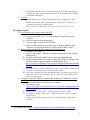
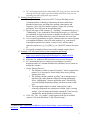
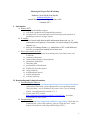
Phonological CorpusTools Workshop
Kathleen Currie Hall & Scott Mackie
[email protected]
Annual Meeting on Phonology, Vancouver, BC
9 October 2015
I. Introduction
A. What is PCT?
i. a free, downloadable program,
ii. with both a graphical and command-line interface,
iii. designed to be a search and analysis aid for dealing with questions of
phonological interest in large corpora
B. A corpus?
i. a list of words with other possible information about each: e.g., its
transcription, its frequency of occurrence, its lexical category, its syllable
structure, etc.
ii. these are in columnar format, e.g., loaded from a CSV or tab-delimited
text file, or created from running text of some sort
C. Basic functionality includes:
i. simple creation of corpora from running texts, inter-linear texts, and
TextGrids
ii. summary information
iii. featural interpretation of transcriptions
iv. phonotactic probability
v. functional load
vi. predictability of distribution
vii. Kullback-Leibler divergence
viii. string similarity
ix. neighbourhood density
x. mutual information
xi. acoustic similarity
II. Downloading and Getting Information
A. Downloading the software:
i. Go to https://github.com/PhonologicalCorpusTools/CorpusTools/releases
and download the latest version appropriate to your operating system
(.dmg for Macs; .exe for Windows; the source code if you’re running
Linux). Currently the latest version is 1.1.1.
ii. See the main PCT website,
http://phonologicalcorpustools.github.io/CorpusTools/, for further
instructions for each system.
B. Documentation:
i. user's manual: http://corpustools.readthedocs.org/en/latest/ (Note that you
can download a .pdf of this guide by going to "Read the Docs" on the
bottom left-hand side of the page and selecting "PDF.")
1
ii. Documentation can also be found throughout the PCT software itself by
clicking on "Help" (either in the main menu or in dialogue boxes relating
to individual functions).
C. Citation:
i. Hall, Kathleen Currie, Blake Allen, Michael Fry, Scott Mackie, and
Michael McAuliffe. (2015). Phonological CorpusTools, Version 1.1.0.
[Computer program]. Available from:
https://github.com/PhonologicalCorpusTools/CorpusTools/releases.
III. Sample Corpora1
A. Five possible ways to get a corpus into PCT:
i. use a built-in corpus
ii. use a pre-formatted (e.g., CSV or tab-delimited) corpus file on your
computer
iii. create a corpus file from running text
iv. create a corpus file from Praat TextGrids
v. import a corpus from your own local copy of another standard corpus
(currently, we support the Buckeye corpus and the TIMIT corpus)
B. Built-in corpus (requires internet connection for initial access):
i. go to the “File” menu
ii. select “Load corpus...” from the list, which will open the “Load corpora”
dialogue box
iii. click on “Download example corpora” from the right-hand menu
iv. download either of the two example corpora (one is called “example” and
the other called “Lemurian” (both are entirely made up; see
http://corpustools.readthedocs.org/en/latest/examplecorpora.html#example
-corpora) and/or the IPHOD corpus (Vaden et al. 2009)
v. the corpus appears in the lefthand side of the “Load corpora” dialogue box
vi. select the corpus and click on “Load selected corpus”
vii. Once these corpora have been downloaded once, you don’t have to do so
again; they will be saved automatically to your local system unless and
until you delete them.
C. Creating a corpus file from pre-formatted file, running text, TextGrids, or other
standards:
i. can be created from local files on your computer
ii. for examples, go to
https://www.dropbox.com/sh/v4l29isywe532an/AAB_a1mQqaEzBpirEY6
a62Xha?dl=0 (this is the entire folder; see also below for individual links)
iii. Go to “File” / “Load corpus...” and then choose “Import corpus”
iv. select the file using “Choose file...” and navigating to it from a system
dialogue box
v. Enter a name for the corpus in the box to the right of the corpus source
selection
1
see complete info. at http://corpustools.readthedocs.org/en/latest/loading_corpora.html
2
vi. PCT will automatically detect what kind of file type you have selected and
select the tab for the corpus type that it thinks most likely, but you can
manually select the appropriate type instead.
D. Setting Parsing Parameters:2
i. For any new corpus, you need to tell PCT what will belong in each
column and where it should get information for that column from.
Standard column types are things like spelling, transcription, and
frequency. Once you have started to import a corpus, the “parsing
parameters” box will open on the right-hand side.
ii. Specify the name of the column (e.g., “Spelling”), its annotation type (e.g.,
“Orthography”), how it should be associated with words (e.g., does this
get associated to single lexical items or should it be allowed to vary within
lexical items), and what delimiters or special characters are to be used.
iii. You can specify punctuation to ignore, characters that are used as segment
or morpheme delimiters, what to do with numbers (e.g., treat them as
transcription symbols, tone marks, or stress levels), and any multicharacter sequences (e.g., [ei], [SH], [i:], etc.) that PCT needs to be aware
of.
iv. See specific examples of these issues in the example corpora below.
E. Example: CSV file; basic feature system assignment and editing:
i. download the following file to your local machine:
https://www.dropbox.com/s/rig9sl60lwie4gb/csv_sample.txt?dl=0
ii. “File” / “Load corpus” / “Import corpus”
iii. Select the csv_sample.txt file from wherever you saved it in step i.
iv. PCT automatically gives it a name (you can change if you like);
determines that it is a column-delimited file; and that it uses a comma to
delimit the columns.
v. Under “Parsing Preview”:
1. The frequency column is named “frequency” and is assigned to be
numeric; it is associated to lexical items; there are no parsing
settings to be used.
2. The spelling column is named “spelling,” but is interpreted as a
character type, rather than the column specifying orthography.
Select “Orthography” from the pull-down menu. Theoretically,
you could change the parsing settings, but there are none in this
case.
3. The transcription column is named “transcription” and is
accurately interpreted as a transcription column. Under “parsing
settings” you can change the delimiter, though PCT has correctly
automatically interpreted the period as the symbol to use.
vi. Click “Ok.” The “csv_sample” corpus appears in the list of available
corpora. Click on it and choose “Load selected corpus.”
2
see more at http://corpustools.readthedocs.org/en/latest/loading_corpora.html#parsingparameters
3
vii. Click on “Corpus” / “Summary.” The inventory is listed alphabetically.
This is because there is no feature system associated with the symbols;
PCT does not yet know how to interpret the transcriptions. Click “Done.”
viii. Go to “File” / “Manage feature systems” / “Download feature systems.”
ix. Select “IPA” as a transcription system and “Hayes” as a feature system
and click “OK.” The “ipa2hayes” file appears in “Available feature
systems.” Click “Done.”
x. To actually associate this feature system with this corpus, go to “Features”
/ “View / change feature system.” Select “ipa” as the transcription system
and “hayes” as the feature system. The system will appear.
xi. To verify, click “Check corpus inventory coverage.” You should get a
message that “All segments are specified for features.” Click “OK.”
xii. Click “Save changes to this corpus’s feature system.” Note that in the
corpus view, the feature system is now visible on the bottom right-hand
corner of the screen.
xiii. Click on “Corpus” / “Summary.” The inventory is now displayed as an
IPA chart. Note that [ɑ] is not listed as an open vowel but rather as an
unclassified segment. Click “Done.”
xiv. Go back to “Features” / “View / change feature system.” Click on “Edit
inventory categories.” Under “Vowel height,” mouse-over the box next to
“Open” vowels; [ɑ] is correctly included here. Under “Vowel backness,”
mouse-over the box next to “Back” vowels; [ɑ] is missing here. Currently,
back vowels are set to be those that have all three feature specifications
[+back, +tense, -front]. Remove [+tense] and note that the inventory will
now include the low vowels (along with many other segments, including
non-vowels; these are excluded under “Major distinctions”). Click “Ok”
and “Save changes to this corpus’s feature system.”
xv. Click on “Corpus” / “Summary.” The IPA chart now correctly places [ɑ]
as a low back unrounded vowel.
F. Example: Running text with non-delimited digraphs:
i. download the following file to your local machine:
https://www.dropbox.com/s/vzqapktuvspoval/running_text_sample_nonde
limited_digraphs.txt?dl=0
ii. This is a running text file with a bunch of transcribed words in it. Some of
them repeat multiple times; some of them have morphological boundaries
indicated.
iii. “File” / “Load corpus” / “Import corpus”
iv. Select the running_text_sample_nondelimited_digraphs.txt file from
wherever you saved it in step i.
v. PCT automatically gives it a name (you can change if you like).
vi. PCT erroneously attempts to make it a column-delimited file; select
“Running text” instead.
vii. Specify that the text type is “Transcription.”
viii. If you’ve already downloaded the ipa2hayes transcription system (steps
viii and ix of the CSV sample above), select this as the transcription
system.
4
ix. Under “Parsing preview” make sure “Transcription” is selected as the
annotation type.
x. Under “Edit parsing settings” select “Check all” to treat both [-] and [=] as
morpheme boundaries.
xi. Under “Multi-character segments,” select “Construct a segment.” The
characters in the .txt file are automatically detected and listed here
alphabetically. Select “s” and “h” to indicate that [sh] should be treated as
a single multi-character segment. Click “Add.” (You could also just type
this in to the multi-character segment box, or copy-and-paste from another
location. Note that all multi-character segments for the built-in
transcription systems are listed on the main PCT website for easy access.)
xii. Click “OK” in the parsing settings. Note that the morpheme delimiters and
the multicharacter segment [sh] will now appear in the “Parsing preview”
window. Click “Ok.”
xiii. Select the “running_text_sample_nondelimited_digraphs” from the
available corpora and click “Load selected corpus.”
xiv. PCT back-creates spelling based on the transcriptions. The transcriptions
are listed with delimiters. Note that [sh] is correctly treated as a single
segment. Frequencies are based on the number of occurrences in the text
file.
xv. On the right-hand side, the original text is shown in its original order.
xvi. Click on “Corpus” / “Summary.” The inventory is basically displayed in
an IPA chart (if you used the ipa2hayes feature system during import).
But, [sh] is not a standard IPA symbol, so it is listed as unclassified. Click
on “Done.”
xvii. Go to “Features” / “View / change feature system.” If you select “Check
corpus inventory coverage,” it will specify that [sh] is missing. Click “Add
segment” and put ‘sh’ in the “Symbol” box (without quotation marks).
You can go through and specify all the features you would like for this
symbol.
1. Assuming this is supposed to be like [ʃ], the values are as follows.
It’s probably easiest to set them all to [-] first: [-ant, -approx,
0back, +cons, -cg, +cont, +cor, +delrel,3 0diph, +dist, -dors, 0front,
0front-diph, 0high, -lab, -labiodental, -lat, -long, 0low, -nas, round, +seg, -son, -sg, -stress, +strid, -syll, -tap, 0tense, -trill, voice].
xviii. Click “Ok.” Click “Save changes to this corpus’s feature system.”
xix. Go back to “Corpus” / “Summary.” [sh] is now correctly listed as a
voiceless alveopalatal fricative.
G. Example: Inter-linear texts:
i. download the following file onto your local machine:
https://www.dropbox.com/s/imcbdstbd7ar588/ilg_example.txt?dl=0
3
[S] is listed as [+delayed release] in the Hayes feature system used here. You are of course free
to edit the feature specifications to your own liking.
5
ii. This is a running text file, but this time the lines alternate between being
“orthographic” lines and “transcribed” lines. The difference between lines
is not marked.
iii. “File” / “Load corpus” / “Import corpus”
iv. Select the ilg_sample.txt file from wherever you saved it in step i.
v. PCT automatically gives it a name (you can change if you like).
vi. PCT erroneously attempts to make it a column-delimited file; select
“Inter-linear text” instead.
vii. PCT automatically detects the number of lines per gloss (in this case two,
one for orthography and one for transcription). You can manually correct
this if it is inaccurate.
viii. Under “Parsing preview,” you can specify how PCT should interpret each
line of the text. The defaults in this case should all be accurate. That is, the
first line is interpreted as Orthography and the second as Transcription.
The transcription line is automatically detected to have period delimiters
between characters.
ix. If you’ve already downloaded the ipa2hayes transcription system (steps
viii and ix of the CSV sample above), select this as the transcription
system. Click “Ok.”
x. Select the “ilg_sample” from the available corpora and click “Load
selected corpus.”
xi. As with running text, you get two panes; the one on the left shows the
standard corpus (spelling, transcription, frequency), and the one on the
right shows the original text in order.
xii. The same issues with assigning features and checking inventory coverage
as in the CSV example (vii-xv) apply here.
H. Example: TextGrids and pronunciation variants:
i. download the following entire folder and its contents onto your local
machine: https://www.dropbox.com/sh/45z2qft338siae8/AAA9WX7Ehhaqh1Sg5is0Ag8a?dl=0
ii. “File” / “Load corpus” / “Import corpus”
iii. Select the TextGrid_sample folder from wherever you saved it in step i
(use the “choose directory” option instead of the “choose file” option,
because in this case we are trying to create a corpus from multiple separate
TextGrid files; one could also create a (very small) corpus from a single
TextGrid)
iv. Assuming that the majority of the files in the directory are in TextGrid
format, PCT will automatically recognize the format and select it.
v. These TextGrids were created using a .wav file of a read story and a .txt
file of the story contents. The TextGrids were generated automatically
using WebMAUS (https://webapp.phonetik.unimuenchen.de/BASWebServices/#/services). WebMAUS by default creates
three tiers: a spelling tier (abbreviated ORT), a canonical pronunciation
tier (abbreviated KAN), and a tier indicating the interpreted pronunciation
by WebMAUS (abbreviated MAU). These three tiers each appear in the
“Parsing Preview” window. Here is an example of the original TextGrid:
6
1. The ORT tier should be specified as “Orthography” under
annotation type. Each element is associated to a lexical item.
2. The KAN tier should be specified as “Transcription.” Again, each
element is associated to a lexical item. The parsing settings should
be edited. Here, there are no delimiters between elements and as
can be seen from the above screenshot, the transcription system
involves some multi-character sequences. The basic transcription
system for WebMAUS is SAMPA, so we’ll want to include all of
the multi-character SAMPA sequences in PCT’s parsing. Because
SAMPA is one of the built-in feature systems, you can get a list of
the multi-character sequences in it from the main PCT website:
http://phonologicalcorpustools.github.io/CorpusTools/. Scroll
down to the section on multi-character sequences and copy the list
given. In PCT, paste the list into the box under “Edit parsing
settings” / “Multi-character segments.”
3. The MAU tier should also be specified as “Transcription.” This
time, however, you should allow the property to vary across lexical
items to allow individual words to have multiple pronunciation
variants. Under “Edit parsing settings,” we want to specify that the
TextGrid boundaries are being used as delimiters between
segments. We can do this by entering a single space character in
the “delimiter” box (the preview at the top indicates that it is a
space that is being used to delimit characters).
7
vi. If you had already downloaded the SAMPA transcription / feature system,
you could specify that it should be associated with the corpus, but if not,
you can leave it blank and add it later.
vii. Click “Ok.” Select the “TextGrid_sample” from the available corpora and
click “Load selected corpus.”
viii. The corpus has three panes:
1. On the left is the list of individual TextGrids, which are interpreted
as separate speakers. Select one from the dropdown menu; that is
how the right-hand window will be populated.
2. In the centre is the standard “corpus” view, which includes the
orthography, canonical transcriptions, and frequency of occurrence
across all files in the sample. Note that the transcriptions are now
period-delimited and should recognize all the multi-character
segments you added above.
3. On the right is the running text for this particular TextGrid. You
are given the orthography, surface transcription, and time stamps
of each word.
ix. To associate a feature file for this TextGrid corpus, which uses SAMPA
transcriptions, follow steps viii-xii from the CSV example above, but
select “X-SAMPA” as the transcription system in step ix.
x. To see the pronunciatioin variants for a specific item, right-click on that
item and select “List pronunciation variants.” For example, the word “He”
occurs 8 times in this corpus; it is apparently produced as [hi:] 6 times and
as [hI] twice. (Note that PCT is case-sensitive; there are a separate 38
occurrences of “he.” To collapse these, we would need to make sure that
the words were not differentiated in the original TextGrid orthography
tier.)
I. Example: Buckeye corpus:
i. download the following entire folder and its contents onto your local
machine:
https://www.dropbox.com/sh/oti1842xc21rcgj/AACFgWrnVhkLnWO0W
KJvxUzSa?dl=04
ii. “File” / “Load corpus” / “Import corpus”
iii. Select the Buckeye_sample folder from wherever you saved it in step i
(use the “choose directory” option instead of the “choose file” option,
because the Buckeye corpus has multiple files and multiple file types)
iv. Assuming that the majority of the files in the directory are in Buckeye
Corpus format, PCT will automatically recognize the format and select it.
v. The default settings under “Parsing Preview” should be accurate. In
particular, note that the “Transcription” level is set to be associated with
lexical items (these are the canonical forms) while the “Surface
4
To get access to the complete Buckeye Corpus, please go to http://buckeyecorpus.osu.edu and
request access to the entire corpus. You can download the entire thing to your local directory and
then follow the same steps listed here to create the corpus in PCT.
8
Transcriptioin” level is set to vary within lexical items (these include
whatever pronunciation variants were used during specific productions).
vi. Click “Ok.” The “Buckeye_sample” corpus appears in the list of available
corpora. Click on it and choose “Load selected corpus.”
vii. As with the TextGrid example, the corpus has three panes.
1. On the left is the list of individual speakers. In the sample we’ve
provided here, only one speaker exists, but you can still select it
from the dropdown menu; that is how the right-hand window will
be populated.
2. In the centre is the standard “corpus” view, which includes the
orthography, canonical transcriptions, and frequency of occurrence
across all files in the sample. Note that the first several entries have
no transcriptions; these can be hidden by right-clicking and
selecting “Hide non-transcribed items.”
3. On the right is the running text for this particular speaker. Again,
the first part tends to be non-transcribed vocalizations; scrolling
down gets you to the meat of the transcript. You are given the
orthography, surface transcription, and time stamps of each word.
You can also select a word or multiple (contiguous) words and
listen to the sound files.
viii. To associate a feature file for the Buckeye corpus, follow steps viii-xii
from the CSV example above, but select “Buckeye” as the transcription
system in step ix.
J. Other information about feature systems:
i. You can use any transcription-to-feature system you like. Just create it as a
spreadsheet file and upload it. For complete information, see
http://corpustools.readthedocs.org/en/latest/transcriptions_and_feature_sys
tems.html.
IV. Sample Analyses
Rather than giving you details of how to do analyses, we refer you to the PCT
documentation, which gives extensive illustrated information on how to use PCT to
conduct various analyses, including information on how to select sounds, define
environments, set options, and save results. The documentation also includes references
to the original sources for each analysis technique and explanations of how / when to use
them.
We recommend starting with phonological search
(http://corpustools.readthedocs.org/en/latest/transcriptions_and_feature_systems.html#ph
onological-search) and then moving on to a segment-based analysis such as functional
load or predictability of distribution, a word-based analysis such as phonotactic
probability or neighbourhood density, and then trying the acoustic similarity analysis
functions.
9
One example analysis: Quantifying allophony using predictability of distribution (additionally
illustrates segment / feature selection):
i.
Using the steps in III-B above, download and open the “Example” corpus.
ii.
See details about how this corpus was constructed here:
http://corpustools.readthedocs.org/en/latest/examplecorpora.html#the-example-corpus
iii.
The pattern: In the example corpus, [e] and [o] are allophones of [i] and [u], respectively,
which occur only immediately before a nasal consonant.
iv.
To confirm or quantify this state of allophony, use the metric of predictability of
distribution (Hall 2009). For each pair of sounds, this returns a value that ranges from 0
to 1; 0 = no uncertainty, i.e., perfect complementary distribution; 1 = complete
uncertainty, i.e., perfect overlapping distribution.
v. “Analysis” / “Predictability of distribution”
vi.
We’re interested here in the relation between mid vowels on the one hand and high
vowels on the other, rather than just a single pair of segments. Hence, select “Add pair of
features” rather than “Add pair of segments.”5
vii.
The feature that distinguishes the mid vowels from the high vowels is [high]. Type in
‘high’ (no quotation marks) in the “Feature to make pairs” box. (Note that as you type,
the list of possible features that match your current typing appears.)
viii.
All pairs of sounds distinguished by that feature are listed. In this case, that covers the
sounds we are interested in and no others; one could also add filters to the pairs to
eliminate extra ones (e.g., [-low] if there had been low vowels in this set too).
ix.
Click “Add.” The chosen sets appear on the left.
x. We now define environments. The central rectangle marks the “target” of the
environment and has an underscore at the top and a set of empty curly brackets, {},
beneath. On either side of the central target rectangle, there is a “+” button. These allow
you to add segments to either the left-hand or the right-hand side of the environment in an
iterative fashion, starting with segments closest to the target and working out. Clicking on
one of the “+” buttons adds an empty set {} to the left or right of the current environment.
To fill the left- or right-hand side, click on the rectangle containing the empty set {}. This
brings up the sound selection box.6 The environment can be filled by either clicking on
segments or specifying features. The relevant environments in this case might be
[_[+nas]], [_[-nas]], and [_#]. For this analysis, you want to ensure that your environment
selection is exhaustive and non-overlapping. For more information, click the “About
predictability of distribution...” button.
i.
Other options can be set if available. For example, the analysis could be done on some
tier of the corpus other than the whole transcription, if one has been created (e.g., a vowel
tier). The analysis could take into account pronunciation variants if the corpus encodes
them. And the analysis can be done using either type or token frequencies of occurrence.
Again, these options are detailed in the relevant Help files and in the original
documentation for this analysis technique.
5
This label is a misnomer. You’re adding a pair of sets of segments, defined featurally. We will
update the button label in the next version.
6
See http://corpustools.readthedocs.org/en/latest/sound_selection.html#sound-selection for
details on how to interact with these boxes.
10
ii.
iii.
Click “Calculate predictability of distribution (start new results table).” The results
appear on screen. You are shown the sounds, the environments, the frequency of
occurrence in each environment, and the entropy (the measure of predictability). As
expected, the sounds are entirely in complementary distribution, with mid vowels
occurring always and only before nasals, so the entropy in each environment (and on
average) is 0.
The results can be saved to a tab-delimited .txt file for later referral or analysis by
selecting “Save to file.” They can also be copied and pasted directly into another
document.
11