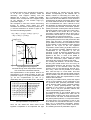
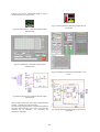
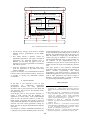
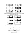
1
Redactor şef / Editor in chief Prof.dr.ing. Ioan Naforniţă Colegiul de redacţie / Editorial Board: Prof. dr. ing. Virgil Tiponuţ Prof. dr. ing. Alexandru Isar Conf. dr. ing. Dan Lacrămă Conf. dr. ing. Dorina Isar Prof. dr. ing. Traian Jurcă Conf. dr. ing. Aldo De Sabata As. ing. Kovaci Maria - secretar de redacţie Colectivul de recenzare / Advisory Board: Prof. dr. ing. Ioan Naforniţă, UP Timişoara Prof. dr. ing. Monica Borda, UT Cluj-Napoca Prof. dr. ing. Brânduşa Pantelimon, UP Bucureşti Prof. dr. ing. Ciochină Silviu, UP Bucureşti Prof. dr. ing. Dumitru Stanomir, UP Bucureşti Prof. dr. ing. Vladimir Creţu, UP Timişoara Prof. dr. ing. Virgil Tiponuţ, UP Timişoara Buletinul Ştiinţific al Universităţii "Politehnica" din Timişoara Seria ELECTRONICĂ ŞI TELECOMUNICAŢII TRANSACTIONS ON ELECTRONICS AND COMMUNICATIONS Tom 46(60), Fascicola 1, 2001 SUMAR ELECTRONICĂ APLICATĂ Lucian A. Jurcă: "Using Masked Logarithm Method for Fast Multiplication and Division Logarithmic Unit Design"… … … … … … … … … … … … … ...… … … … . 3 Lucian A. Jurcă, Beniamin Drăgoi: "Using 4:2 L Compressor in Partial Product Reduction Tree for Fast Binary Multipliers"… … … … … … … … … … … … … ... ... ... ... ... … … ... 11 Avram Ionel Adrian: "Phycal Causes of Integrated Circuits Behaviour Degradation under Ionising Irradiation"… … … … … … … … … … … … … ...… … … … … … 17 INSTRUMENTAŢIE Mihaela Lascu : "Analog Input LabVIEW Applications for Measuring Temperature"…………………… ... ... ... ... ... ... ... ... … … … … … … … … … 19 Septimiu Mischie, Alimpie Ignea : "Implementation of an AC Bridge using a Lab PC+ Data Acquisition Board"…………………… ... ... ... ... ... ... ... ... … … … … … … … … … … … .23 Daniel Belega, Septimiu Mischie : "Considerations Concerning the Practical Behaviour of a Digitising Oscilloscope in Different Signal Recording Modes"…………………… ... ... ... .27 1 TELECOMUNICAŢII Muguraş D. Mocofan, Corneliu I. Toma: "New Interactive Multimedia Application Model Using Objects Storage in a Database".……………………….. ... ... ... ... ... ... ... ... ... ... ... ... ... ... ... ... 31 Ioan Şnep, Dan L. Lacrămă, Corneliu I. Toma: "Optimised Homotropic Structuring Element for Handwriting Characteres Skeleton"… … … … … … … … … … … … … ... ... ... ... ... ... ....37 Andrei Cubiţchi: "Une méthode nouvelle pour la compression de la parole"… … … … ..41 Corina Botoca: "Romanian Bank-Notes Recognition Using Cellular Neural Networks"… … … … … … … … … … … … … … … … … … … … … … … … … … … … .47 Konrad V. Pfaff: "Evaluating Objective Audio Quality for Minidisc and Influence of Multiple Generations Audio Coding for Perceptual Quality"… … … … … ….51 2 Buletinul Ştiinţific al Universităţii "Politehnica" din Timişoara Seria ELECTRONICĂ şi TELECOMUNICAŢII TRANSACTIONS on ELECTRONICS and COMMUNICATIONS Tom 46(60), Fascicola 1, 2001 Using Masked Logarithm Method for Fast Multiplication and Division Logarithmic Unit Design Lucian A. Jurca1 Rezumat – În lucrare este prezentata o metodă originală de structurare a arhitecturii unei unităţi de calcul logaritmice, denumită metoda logaritmului mascat, ce permite efectuarea foarte rapidă a operaţiilor de înmulţire şi împărţire în simplă precizie. Viteza de calcul, superioară altor realizări prezentate în literatura de specialitate, se obţine în condiţiile în care aria ocupată pe cip şi erorile de calcul sunt mai mici decât în cazul referinţelor studiate. Cuvinte cheie: unitate de calcul logaritmică, format LNS, format virgulă flotantă, simplă precizie. n=i+f antithe two and A × B = antilog(logA + logB) (1) A / B = antilog(logA – logB) (2) In fact, through performing a logarithmic and antilogarithmic operation we accomplish the format conversion from floating-point format (FP) into logarithmic format (LNS – Logarithm Number System) and vice-versa. Thus a binary number A in FP system, in single precision format is written: A = (-1)S (1 + 0.M) 2E-127 (3) where S represents the sign bit, M - the normalized mantissa, represented on 23 bits and E - the biased exponent, represented on 8 bits. In the Logarithm Number System (LNS) a binary number z is represented: z = (-1)Sz 2Nz NZ = IZ + FZ (5) The only deficiency of the LNS processors is that they so far permit only single precision computation and zero is not representable in the LNS. For system compatibility, a simple but slightly inefficient encoding is used. Zero is represented by a distinct bit Z in the LNS. When the bit Z is set to 1, the number is zero, regardless of all other bits in the value. Thus i=8 and f=23, which including the bit Z and the sign bit, corresponds to 33 bits [3]. Considering the normalized mantissa (1+0.M) in the domain [1,2), the “biased” integer part of the logarithm of the number is given by the very value of the biased exponent and the fractional part by the logarithm of the mantissa. This concatenation is possible because the binary logarithm of the normalized mantissa is always a positive fractional number. The calculation of logarithm and antilogarithm use the partition of the argument and the memorising of only certain values for reducing the amount of memory and, in addition, we apply a correction method based on the memorisation in the same points of the values of the function derivative too, after which the interpolation is performed [1], [2]. Thus we note y = 0.M and we partition the mantissa y in two parts: y1 containing the most significant 11 bits and y2 containing the least significant 12 bits. The values of the function log(1+y)-y in these 211 = 2048 points are memorised in internal ROM (ROMA) as correction values Ey provided through the application of the address y1. Thus we obtain the following approximation: I. INTRODUCTION The circuits for computing logarithms and logarithms allow the performing of multiplication and division operations of operands A and B by means of addition subtraction operations: and log (1+y) ≅ y + Ey ± ∆Ey × y2 (6) The second look-up table (ROMA’) of the memory is much smaller because ∆Ey << Ey. Considering for ∆Ey a 12-bit representation, the complete conversion between the two formats is made through a reading in the look-up tables, two 23-bit additions and a 12×12 bit multiplication. (4) where SZ is the sign bit and NZ is a fixed-point number having n bits, out of which i bits for the integer part IZ, and f bits for the fractional part FZ. We have: 1 Facultatea de Electronică şi Telecomunicaţii, Departamentul Electronică Aplicată, Bd. V. Pârvan Timişoara 1900 e-mail [email protected] 3 -in the third stage of the structure, there are two successive proper additions, (which, together, lead to a unique final result), consuming a lot of time for the horizontal carry propagation; -ALU operated with data of any polarity, which complicated its control logic and led to a further delay. Later on, the same author presented a new architecture in which the product Ey×∆Ey was calculated not with binary multipliers but with PLA circuits [3], which permitted a saving of area on the chip, however maintaining the same computation speed. Considering these disadvantages, this paper proposes a new method of logarithmic unit design, which does not give up the multipliers and leads to a substantial increase of the calculation speed of at least 1.6 times, resulting an occupied area which is smaller than in [1] and comparable to [3]. The calculation of the antilogarithm is made in the same way. Considering C the result of finding the antilogarithm we can write: C = 2E ±127 + 0.M = 2E ±127 2y (7) where E represents the integer part in LNS format and M represents the fractional part. In this approach we do not extract the bias value from the exponents of the two operands. For this we extend the ALU with one bit to the left, while the bias value is extracted or added to the resulted exponent, depending on the performed operation, multiplication or division [4], [5]. Obviously, the implementation of the square root operation supposes the extraction of the bias value (just in this case) from one of the two data inputs. Y is partitioned in the same way and we use a ROM (ROMC) for memorising the conversion error Ey in 2048 points, as well as the difference ∆Ey (ROMC’). The final result of conversion is: 2y ≅ (1+y) – Ey ± ∆Ey × y2 II. THE MASKED LOGARITHM METHOD (8) In order to eliminate the disadvantages mentioned above we offered a solution of our own, based on a new method of logarithmic unit design, which we called the “masked logarithm” method. To elaborate this method we considered the following furthers aims: -the new structure should be organised in no more than 6 pipeline stages; -the number of logical gates used on certain pipeline stages should not increase significantly; -the size of the latches between the certain pipeline stages should not increase significantly; -the propagation time on the critical stage of the pipeline should be as close as possible to the physically achievable limit, namely to the access time to the ROM integrated on the chip; -the propagation times on the pipeline stages should be as close as possible. Through this new approach, the terms yA,, EyA,, respectively yB, EyB which are added to the products ∆EyA × y2A, respectively ∆EyB × y2B (see equation 6), will be considered as initial partial products of the above mentioned products. These terms will thus be introduced in the Wallace tree for the reduction of the number of partial products, beside the 12 initial partial products of each product. In this way, we eliminated the final multiplication adders, and the two resulting terms in the lower end of the trees (in the sum and carry sections), will implicitly contain the product value too, distributed between the two sections. Using this redundant representation, the proper values of the two products ∆Ey×y2 will no longer be found in the structure explicitly, thus becoming “masked” values. The problem which is still to be solved is that of the situation in which in equation (6), the term ∆Ey × y2 The correction values Ey, for both log(1+y)-y and (1+y)-2y are represented in figure 1. 0.10 log (1+y) - y y (1+y) – 2 0.08 0.06 0.04 0.02 0.00 0.0 0.2 0.4 0.6 0.8 1.0 Fig.1 The conversion errors between the log(1+y) and y and the (1+y) and 2y Implementing the equations (1), (2), (6) and (8) led to a 6-stage pipeline structure [1], [2], which allowed a 100 MHz clock frequency, in 0.8 µm CMOS technology. However the structure which was obtained has the following disadvantages from the point of view of the computation speed: -The propagation times on the pipeline stages were not the same; -The speed advantage resulted from the vertical carry propagation in the multiplication area, organised in a Wallace tree, was diminished by the time necessary for the proper addition of the last two intermediate partial products (when the carry propagation is horizontal), even if this is done with a fast adder; 4 part of equation (9). Starting from the memory location corresponding to the address 907 of ROMA, instead of memorising the value Ey(n), Ey(n+1) is memorised, i.e. exactly what should have been found at the next address. In each location a supplementary bit will be memorised, called control bit, which takes the value 0 for addresses 0…906, and 1 for addresses 907…2047. If this bit is 1 then the generation of partial products will be done with y2 having the bits reversed, and another pseudopartial product with a size equal to that of the least significant partial product, having the value ∆Ey(n), will be added. If the control bit is 0, then the generation of partial products will be done with y2 unreversed, and the bits “pd” of the first pseudopartial product from figure 3 will all be 0. The Wallace tree will thus have as inputs 15 initial pseudo-partial products and it will provide two data words: “sum” and “carry”. If in this stage we did the proper addition of these, we would obtain the value of the logarithm of the mantissa of each operand applied to the input of the two logarithm computation circuits working in parallel. Further on, the two fractional numbers obtained would be concatenated to the exponents of the two operands, in order to obtain the logarithms of the operands. Finally, the two logarithms would be applied to the ALU, in order to be added or subtracted. However, in this case too, we would have two consecutive proper additions, which slows down the process of obtaining the result. For avoiding this situation, we can also consider the two pairs of data words “sum” and “carry” as pseudo-partial products, and thus they are again introduced in a new reduction block. This will provide, in the end, two data words, the final “sum” and “carry”, which will be possible to be added then, with the help of a fast adder. This final reduction block of the last pseudo-partial products will be included in the ALU as it should act under a control logic to allow the implementation of both addition and subtraction. In this way, the adders which provide the explicit values of the logarithms of the mantissas for the two operands were practically eliminated. These values become hidden, being contained implicitly by the 4 partial pseudo-products, and they contribute to the process of obtaining the final result. That is why this operation method was called “the masked logarithm method”. The implementation of this method leads to the generating of a big Wallace tree which has 30 pseudo-partial products and which has its lower end in the ALU. We used, as reduction blocks for the pseudo-partial products, 4:2 compressor blocks and CSA blocks of 3:2 full adders, in such a way as to obtain the most efficient structure, in which there are no unoperated intermediary pseudopartial products on any of the levels of the tree. The resulting structure is presented in figure 4. is negative and its two’s complement conversion, i.e. of all the 12 partial products, would be necessary. This happens starting from the address 907 to 2047 of ROMA and ROMA’, situation which corresponds to the negative slope on the diagram of the function log(1+y)-y, presented in figure 1. We managed to avoid this severe shortcoming through an artifice, which allows the total elimination of the cases in which the product ∆Ey × y2 must be subtracted. As shown in figure 2, we can write the following equation: _ Ey(n) -∆Ey(n) × y2 = _Ey(n+1)+∆Ey(n) ×( y2+1) = = Ey(n+1)+∆Ey(n) × y2+∆Ey(n) (9) Log(1+y)-y ∆Ey(n)×y2 Ey(n) ∆Ey(n) ∆Ey(n)× _ ×( y2+1) Ey(n+1) _ y2 y2+1 1 2-12 y×211 Fig.2 Negative slope segment achieved through linear interpolation between two consecutive memorised values Ey The implementation of this equation leads to an arrangement of the partial products as they are presented in figure 3. A generic presentation, with “qy” for the complemented “py” bits of y2, respectively with “pd” for the bits of ∆EY, was used. -19-20-21-22-23 -24 -25 -26 -27 -28 -29 -30 -31-32-33 -34 -35 ..0 0 0 0 0 pd pdpdpdpdpdpdpdpdpdpdpd ..0 0 0 0 0 qy qyqyqyqyqyqy qyqyqyqy qy ..0 0 0 0 qyqy qyqyqyqyqyqy qyqyqyqy ..0 0 0 qyqyqyqyqyqy qyqyqy qyqyqy ..0 0 qyqyqyqyqyqyqy qyqyqy qyqy ..0 qyqyqyqyqyqyqyqy qyqyqy qy ..qyqyqyqyqyqyqyqyqy qyqyqy ………………………... Fig.3 A section through multiplication area after the implementation of equation (9) Thus, we can obtain the same result of the logarithm computation if we implement the right 5 y2B y2A Control bit Inverter ∆EyA 0 Inverter Mux(2:1) Mux(2:1) y'0∆Ey Cmpr(4:2) ∆E’yB Partial product generator y'11∆Ey y'10∆Ey yA EyA y'9∆Ey Cmpr(4:2) 0 Mux(2:1) y'2B Partial product generator Cmpr(4:2) ∆EyB Mux(2:1) ∆E’yA y'2A CSA(3:2) Control bit Cmpr(4:2) yB y'11∆Ey y'10∆Ey y'9∆Ey CSA(3:2) Cmpr(4:2) y'0∆Ey EyB Cmpr(4:2) Cmpr(4:2) Cmpr(4:2) Cmpr(4:2) Cmpr(4:2) Cmpr(4:2) Cmpr(4:2) Cmpr(4:2) Fig.4 Wallace tree for pseudo-partial product reduction the function 1+y-2y, presented in figure 1, while it is added in the other cases. As equation (9) can no longer be used, the sum of the two negative terms from equation (8) will be written as follows: The CSA block groups up the terms y and ∆Ey with the most significant partial product of y2×∆Ey, in order to avoid the excessive growth of the size of this block, and so the size of the blocks connected after it as well as that of the wiring. For the antilogarithm computation circuit, the procedure applied is the same, the data words “sum” and “carry” being obtained after only 3 levels of compressors. They are then added with a fast adder in order to obtain the mantissa of the final result from the output of the logarithmic unit. In this case too, we will take measures to avoid the subtraction of the term ∆Ey×y2, but we also take into consideration the fact that in equation (8) the term Ey must be subtracted too. The product ∆Ey×y2 is subtracted in the cases which correspond to the positive slope on the diagram of -Ey(n) - ∆Ey(n)×y2 = -(Ey(n)+∆Ey(n)×y2) = - [Ey(n)+ ∆Ey(n)-∆Ey(n)×(y2+1)] = -(Ey(n)+∆Ey(n))+∆Ey(n)×y2 +∆Ey(n) = -Ey(n+1) +∆Ey(n)×y2+∆Ey(n) (10) Thus, in the ROMC locations from the address 0 to the address 1082 the two’s complement of the quantities Ey(n+1), which should have been found at the next address, as well as the value 1 for the control bit are memorised; from address 1083 to address 2047 (when ∆Ey×y2 is positive) the two’s complement of the values Ey(n), as well as the value 0 for the control bit will be memorised directly. 6 In other words, we maintain the situation of initial carry-in 1 , respectively that of initial carry-in 0 at the two adders which work in parallel, conditioned by the presence of a carry-in equal with 1 at the last 4:2 compressor block, in the case of performing a subtraction. Obviously, this carry-in will be 0 in the case of addition. The carry-in is applied at the input Cin which is not used of the least significant 4:2 compressor. Further on, the length of the last block of the tree, included in the ALU, will be supplemented with 9 bits to the left, for the concatenation of the positive exponents (with the bias value of 127 included, according to the modified algorithm) which represent the biased integer part of the logarithm of the two operands. The fractional parts of the logarithms are “hidden”, being distributed between A1 and A2, respectively B1 and B2 of the two pairs of pseudo-partial products. The concatenation of the exponents will be done at the terms A1 and B1, obtaining the final pseudo-partial products A1 and B1, while in the 9 bit positions of integer part corresponding to A2 and B2 of fractional weight, it will be completed with zeros. Thus we will obtain the other two final pseudo-partial products A2 and B2. The block diagram of the new adder/subtracter, designed with the purpose of the complete implementation of the masked logarithm method, is presented in figure 5. The bit line SOP has the logical value 0 in the case of addition and 1 in the case of subtraction. The three blocks “Invert.” will be transparent when an addition is performed and they will invert the bits of the data from the inputs when a subtraction is performed. The block Selector will select the result from the Adder1 unchanged, in the case of addition, and in the case of subtraction it will select the result from Adder2 or from Adder1 inverted, depending on the MSB of Adder2 [5]. The Adder1 and Adder2 are 36-bit adders. The four least significant bits from the outputs of the two adders will be lost, and thus, at the output of the circuit, we will regain the single precision format plus one bit in the MSB position, which avoids the overflow due to the accumulation of bias values in the case of multiplication. The justification of the 36-bit length for the adders and the compressor block will be done in the next paragraph. The adders are 2-level hybrid adders, with four blocks of 8-b carry look-ahead adders (CLA) plus the most significant block of 4-b CLA in the 1st level and a carry select mechanism in the 2nd level. In the most unfavourable case, the delay due to the carry propagation through the circuit presented in figure 5, was found 4 ns by simulation with MSim program, in 0.5µm CMOS technology. III. ALU DESIGN Due to the fact that we must implement in the ALU, besides addition, the subtraction, too which implies the conversion into a two’s complement of the subtractor (the number which is subtracted from the other term), the last 4:2 compressor block from figure 4 will definitely need to be included in the ALU. It will perform the reduction of the last four pseudo-partial products, after the control logic of the adder/subtracter circuit has intervened on the subtractor. The subtractor is represented by two pseudopartial products, whose addition is no longer performed, exactly with the purpose of increasing the propagation speed of the carry through the logarithmic unit. This means that both terms must be converted in two’s complement code. The avoidance of the reconversion from two’s complement in sign-magnitude code of the result, in the case in which it is negative, is done using the same method as in [6], only modified for 4 operands. We note A1, A2, respectively B1, B2 the 4 pseudopartial products, and A = A1 + A2 represents the subtractend, while B = B1 + B2 represents the subtractor, in the case in which a subtraction is performed. Considering the convention of representing B negated (the data word obtained through the inversion of all the bits of B) as being “/B”, we can write the two terms which are simultaneously computed in the adder/subtracter circuit: A - B = A - B1 - B2 = A + /B1+ /B2 + 2 (11) /(B – A) = A + /B1+ /B2 + 1 (12) Equation (12) can be checked as follows: -in equation (13) below, A - B = - (B - A) = /(B - A) + 1 (13) we replace the term”/(B-A)” with the value obtained from equation (12); -we indeed obtain A - B = (A + /B1+ /B2 + 1) + 1 = A + /B1+ /B2 + 2, i.e. exactly the correct value from equation (11). The principle of the adder/subtracter circuit is the following: -if A-B is positive, it is selected at the output, and the sign bit of the result will be 0; -if A-B is negative, it means that B-A is positive and, at the output, the term /(B-A) negated is selected, i.e. B-A; the sign bit of the result will be 1. In order to apply the method from [6], the equations (11) and (12) are rewritten as follows: A - B = (A1 + A2 + /B1+ /B2 +1) + 1 (14) /(B – A) = (A1 + A2 + /B1+ /B2 +1) + 0 (15) 7 corresponding memory locations. Baring in mind that the error in floating-point single precision format, i.e. the value of the least significant bit provided by any output of the ROMA or ROMC, is 1.2 × 10⁻⁷, it means that to the calculated values of Ey we can add corrections of one LSB, after which they are directly memorised (ROMA), respectively, they are transformed in two’s complements and then memorised (ROMC). Theoretically, the total conversion error can be reduced to half if to the memorised value Ey we add an amount equal with the half of the maximum conversion error, i.e. 1.5 × 10⁻⁷. This amount can not be represented on an integer number of bits, which could have been 1 or 2. The compromise is thus the adding of 1 (one LSB) in those locations for which the conversion error is bigger than one LSB, i.e. bigger than 1.2 × 10⁻⁷. In this way the conversion error, both for logarithm and for antilogarithm computation, decreased to 1.8 × 10⁻⁷. As far as the computation of the product ∆Ey×y2 is concerned, we can notice from figure 3, in which the multiplication area is presented, that, if we perform the calculation of the truncation error, in the most disadvantageous case, when all bits of a smaller or equal order with “-28” (the bits of the right side of the vertical line) are equal to 1, we obtain the value: The maximum propagation time through the Wallace tree which contains three levels of 4:2 L compressors is 3 × 1.1 ns, at which 0.7 ns are added for the generation of the partial products, which leads to a total of 4 ns. A1 A2 B1 B2 Invert. Invert. SOP 36-b 4:2 Compressor Block 36-b Adder1 MSB 0 36-b Adder2 1 32-b Invert. 2×10-35+3×10-34+4×10-33+5×10-32+6×10-31+7×10-30+ +8×10-29+9×10-28 = 5,96×10⁻⁸. 32-b Selector ⎯ SOP A +/- B This value represents half of the representation error in single precision format. The removal of all bits from this area, i.e. the elimination of the hard structures from the whole Wallace tree and ALU which correspond to this area, does not introduce a supplementary error if the values Ey which are memorised in ROMA are rounded to 23 bits toward the nearest higher value, and the values Ey whose two’s complement is memorised in ROMC are rounded through truncation. Fig.5 Block diagram of the ALU (the adder/subtracter circuit) The sign bits of the operands are processed separately in the ALU. The sign bit of the result can be obtained by the implementation of the logical function: SC = SA ⊕ SB (16) V. CONCLUSIONS IV. ERROR ANALYSIS The use of the masked logarithm method in the implementation of the logarithmic unit allows a very efficient organisation in a 6-stage pipeline structure, as shown in figure 6. The total time for the obtaining of the result (we have taken into consideration the maximum propagation times of all the blocks from the critical path) is: After analysing, with the help of the Matlab program, the errors introduced by using the algorithm described in [1] for the generation of binary logarithm and antilogarithm, we had the confirmation of the value of 3 × 10⁻⁷ initially mentioned in [1] as the maximum conversion error. However, this error is of about 2.5 times bigger than the one in single precision format, which is of 1.19 × 10⁻⁷. For the further minimisation of the conversion error, we suggested a solution of our own, which will add correction values on certain address intervals of the ROMA and ROMC, in the ttot = tROMA + tlog.tree + tALU + tROMC + talog.tree+ tFinSum = = 4 ns + 4 ns + 4 ns + 4 ns + 4 ns + 4 ns = = 24 ns. 8 Input operand A (SA, EA, yA) Input operand B (SB, EB, yB) y1B y1A EA yA ROMB, ROMB’ ROMA, ROMA’ EyA ∆EyB ∆EyA y2A A1 B2 A2 SA EyB SOP B1 B2 B1 ALU SB 4ns Wallace Tree - Branch B A2 4ns y2B Wallace Tree - Branch A A1 yB EB SC 4ns IC, FC y1C IC FC ROMC, ROMC’ +/-127 Add./Sub. exp. bias y2C ∆EyC EyC Wallace Tree (antilog.) C1 4ns C2 27-b Carry-Lookahead Adder EC 4ns 4ns yC Output C Fig. 6 The architecture of the logarithmic unit -the number of logical gates from the entire structure is significantly smaller, due to the elimination of 8 fast adders of minimum 18 bits, with the price of the supplementation of three fast adders with 4 bits; -the propagation time through the critical stage of the pipeline decreased up to the minimum physical level, given by the access time of the memories; -the latch size between the pipeline stages decreased with roughly 15%, due to the arborescent structure of the logarithmic unit; We can see that in this case, unlike in the case of the most performant implementation described in the field literature by F. Lai and E. Wu [1], [2], [3], the propagation times through the blocks from the critical path are considerably smaller and are much more balanced. The clock frequency of the system thus reaches 250 MHz, which represents a speed increase of over 60% in comparison with the above mentioned reference. Furthermore, we can notice some other remarkable features: 9 -a supplementary saving, of roughly 25%, was achieved at the implementation of the three multiplication operations of the type ∆Ey×y2 , a possibility which has been demonstrated through an error calculation in the case of the above mentioned product. BIBLIOGRAPHY [1] Lai F., “A 10-ns Hybrid Number System Data Execution Unit for Digital Signal Processing Systems”, IEEE Journal of SolidState Circuits, Vol. 26, No. 4, Apr. 1991, pp. 590-599 [2] Lai F., Wu C.F.E., “A Hybrid Number System Processor with Geometric and Complex Arithmetic Capabilities”, IEEE Transactions on Computers Vol. 40 No.8 Aug.1991, pp. 952961. [3] Lai F., “The Efficient Implementation and Analysis of a Hybrid Number System Processor”, IEEE Transactions on Circuits and Systems, Vol. 46, No. 6 ICSPE5, June 1993, pp 382-392. [4] Jurca L. A., “Some Considerations Regarding the Design of a Hybrid Logarithmic, Floating-Point Mathematical Processor”, Buletinul UPT, Tom 45(59), Fasc. 1, 2000, pp. 169-172 [5] Jurca L. A., “Logarithmic Unit for Fast Performing of Multiplication and Division Operations in Single Precision Format”, Buletinul UPT, Tom 45(59), Fasc. 2, 2000, pp.29-32. [6] Fujii H. & all, “A Floating-Point Cell Library and a 100MFLOPS Image Signal Processor”, IEEE Journal of SolideState Circuits, Vol.27, No.7. July 1992, pp.1080-1088. [7] Mori J. & all “A 10-ns 54×54-b Parallel Structured Full Array Multiplier with 0.5-µm CMOS Tehnology”, IEEE Journal of Solid-State Circuits, Vol.26, No.4, April 1991, pp. 600-605. 10 Buletinul Ştiinţific al Universităţii "Politehnica" din Timişoara Seria ELECTRONICĂ şi TELECOMUNICAŢII TRANSACTIONS on ELECTRONICS and COMMUNICATIONS Tom 46(60), Fascicola 1, 2001 Using 4:2 L Compressor in Partial Product Reduction Tree for Fast Binary Multipliers Lucian A. Jurca1, Beniamin Drăgoi2 Rezumat – În lucrare este prezentat un nou tip de compresor 4:2, denumit compresor 4:2 L ce permite o creştere cu aproximativ 10% a vitezei de calcul a unui multiplicator binar la care produsele parţiale sunt organizate în arbore Wallace. Sinteza compresorului 4:2 L a avut la bază o nouă abordare în definirea acestui tip de circuit, ce a condus la lărgirea familiei din care face parte. Simulările efectuate au dovedit avantajele în ce priveşte viteza de propagare a transportului prin noua structură, realizată în tehnologie CMOS 0,25 micrometri, comparativ cu alte soluţii prezentate în literatura de specialitate. Cuvinte cheie: compresor 4:2, format LNS, format virgulă flotantă, simplă precizie The great computation speed is obtained on the one hand due to the solely vertical propagation of the carry in the multiplication area, and on the other hand due to the simultaneous calculation of more initial or intermediate partial products. But using only CSA blocks leads to the situation in which 1 or 2 partial products remain unoperated on one of the levels of the Wallace tree. This fact results in a certain inefficiency due to the further delay which appears with the increase of the number of levels of the Wallace tree. A more efficient structure is obtained if, instead of the CSA blocks, we use 4:2 compressor blocks or a combination of 4:2 compressors and CSA blocks. The 4:2 compressor was introduced in the field literature by Weinberger in 1981. However, the first implementation on the chip which used this circuit appeared only in 1991, in the form of the 54 × 54 bit multiplier, designed by J. Mori [2], possible to be achieved as a result of the increase of integration density. Since then, other, improved variants of 4:2 compressors have appeared, variants which will be compared at the end of this paragraph with our own variant of this circuit, named the 4:2 L compressor. I. INTRODUCTION The increased level of integration brought by modern VLSI and ULSI technology has rendered possible the integration of many components that were considered complex and were implemented only partially or not at all in the past. The multiplication operation is certainly present in many parts of a floating-point (FP) processor, most notably in signal processing, graphics and scientific computation. Parallel multipliers have even migrated into the fixed-point processor of digital computers for de purpose of speeding up and facilitating address calculation and, more recently, into the hybrid FP-LNS (Logarithm Number System) processors [8], [9], for de purpose of allowing implementation of algorithms needed for format conversion between FP and LNS. The most appropriate multiplier is obtained when the partial products from the multiplication array are grouped into a Wallace tree [1]. Initially, the component blocks of the tree were CSA (Carry Save Addition) blocks, which were made up of independent 1-bit full adders. The CSA blocks accepted 3 partial products at the input and they provided 2 intermediate partial products in a time equal to the one necessary for the propagation through one full adder. II. THE 4:2 COMPRESSOR CIRCUIT The generalised name of “4:2 compressor” does not reflect exactly the features of this circuit because the sum of the 4 input bits of equal weight can not be represented in all possible cases with the help of the two output bits. The circuit also provides a carry-out on a supplementary output line and thus needs an input for the introduction of the carry-in. In this way, there is a “4:2” vertical propagation path and a “1:1” horizontal propagation path. However, the horizontal propagation of the carry is practically limited to 1 bit, because the carry-out is generated in such a way that it does not depend on the carry-in. Thus, on the scale of the whole multiplier, the use of this circuit permits the shift of the critical propagation 1, 2 1 Facultatea de Electronică şi Telecomunicaţii, Departamentul Electronică Aplicată, Bd. V. Pârvan Timişoara 1900 e-mail: [email protected] 2 e-mail: [email protected] 11 -The 3-input NAND gates, in advanced submicronic technologies which need smaller supply voltages, can no longer be implemented, or they are implemented through two 2-input NAND gates, by the addition of one more logical level. In this way the critical propagation path through the circuit becomes the one which includes the fast output Cout of the current compressor and the input Cin and the output Carry of the left-hand compressor. So, this path becomes slower compared to the propagation time for “x1” and “x2” (figure 1) through 3 successive OR-exclusive gates. Even in technologies which allow the integration of 3-input NAND gates, its propagation time is bigger than through a 2-input gate. -The use of unconventional OR-exclusive gates [2], faster than the classical ones, having tP(OR-excl) < 2tP(NAND), will not bring the expected advantages because the propagation through 3 OR-exclusive gates in cascaded configuration no longer represents a critical path in the compressor. -There are lots of cases in which the capacitive load of a logical output is considered to be excessive when it appears on a critical propagation path. Thus, there are cases in the structure of the compressor in which an output commands three inputs, i.e. minimum six MOS gates. To the intrinsic capacity of these, there is added the parasite capacity of the three signal paths. path from the centre of the multiplication area (where the degree of partial product overlap is the maximum) towards the left end (where this degree of overlap becomes less and less). Furthermore, the combination of CSA blocks of 3:2 full adders and 4:2 compressor blocks allows an efficient design of the Wallace tree, by the elimination of the cases in which one or two initial or intermediate partial products remained ungrouped cross a level of the tree without being operated [5]. The number of levels of the Wallace tree thus becomes smaller and the critical propagation path is also shorter. In principle, a 4:2 compressor is obtained through the interconnection of two 3:2 full adders, whose structure is presented in figure 1 doubly and which presents a propagation time equivalent to 4 ORexclusive gates in cascaded configuration. A major improvement of the structure of the 4:2 compressor was brought by D. Villeger in [3] and [6], by the exploiting of the “fast” inputs and outputs of the 3:2 full adders, in such a way that the maximum propagation time becomes the equivalent of only 3 OR-exclusive gates in cascaded configuration. This optimised structure is presented in figure 1. For this compressor, the 4 input bits are x1, x2, x3 and x4, while the 2 output bits are Sum and Carry. The carry-in is Cin and the carry-out is Cout. The Carry and Cout bits have a double weight in comparison with Sum. The Sum bit is obtained through the implementation of the OR-exclusive function between the 5 inputs of the circuit. Supposing that the propagation time of the carry through an OR-exclusive gate is twice bigger than through an NAND or NOR gate, we can notice in figure 1 that, indifferent of the propagation path of the input signals, including the Cin generated by the right-hand compressor, the maximum propagation time is not longer than the equivalent of 6 simple logical gates or 3 OR-exclusive gates. We can also notice that the output Cout does not depend on the input Cin, and so the propagation of the carry on the horizontal in the compressor block from figure 2 is limited to a single bit (single position) to the left. The vertical propagation time of the whole block is actually the vertical propagation time through one compressor. This obviously means that the reduction to half of the number of partial products is made in a time equal to the propagation time on the critical path through the 4:2 compressor. For this reason, the fast propagation of signals through this circuit is essential and practically determines the propagation speed through the whole Wallace tree. The optimised 4:2 compressor, described in [6] and presented in figure 1, has a series of limitations which affect the propagation time of the carry: III. THE 4:2 L COMPRESSOR The elimination of the above mentioned disadvantages was made by the design of our own variant of 4:2 compressor, presented in figure 3, which is 10% faster than the compressor presented in [6], as proved by simulation. Considering the fact that in a 54 × 54-bit multiplication array there are 5 levels of 4:2 compressors, this leads on the whole to a saving of 0.35 ns (in 0.25 µm CMOS technology). In the design of our own variant we started from the idea of finding a general definition for the 4:2 compressor, whose inputs and outputs are already defined. Thus, this circuit has to provide the following functions: a) the output Sum has to be generated by the equation (1): Sum = x1 ⊕ x2 ⊕ x3 ⊕ x4 ⊕ Cin (1) b) the two outputs Carry and Cout have to be of an immediately superior order to Sum (to have a double weight), so that the maximum sum of the 5 input bits, which equals 5, could be represented. In this way, the equation (2) will be satisfied: x1+x2+x3+x4+Cin = Carry+ Cout+ Sum (2) Indeed, when all the input bits are 1 we obtain: 5=102+102+1. 12 Fig. 1 Optimized 4:2 compressor, presented in [6] x1k x2k x3k x4k 4:2k+2 4:2k+1 Coutk Carryk 4:2k Cink 4:2k-1 Sumk “CARRY” BITS Fig. 2 Section through a 4:2 compressor block Fig. 3 The 4:2 L compressor 13 “SUM” BITS disadvantage of supplementary capacitive load of certain logical outputs (one output does not command more than two inputs) and, in the same time, it permitted the implementation of the De Morgan equations for the exclusive use of intrinsic gates in CMOS technology. Because the outputs Cin and Carry have the same order, they provide a redundant representation at the output of the 4:2 compressor. c) One of the bit lines of output carry has to be generated by simple logical functions, which to include a minimal number of logical levels and not to depend on the carry-in Cin. It will be called fast output and will insure the carry-in for the compressor with the immediately superior order. In this way the horizontal propagation of the carry will be limited to only one bit and will not influence the speed of result generation at the output of a cascaded 4:2 compressor block. d) All possible combinations of input bits for which their sum is 0 or 1 have to lead to Carry = Cout = 0. e) All possible combinations of input bits for which their sum is 2 or 3 have to lead to Carry= 1 and Cout = 0, or Carry= 0 and Cout = 1. In other words, all these possible combinations which produce either Carry= 1 or Cout = 1 have to be found in two disjuncted areas. This possibility insures the redundant character of the outputs of the circuit. Exploiting of this property, we will be able to enlarge the family of 4:2 compressors. f) All possible combinations of input bits for which their sum is 4 or 5 have to lead to Carry = Cout = 1. Taking into consideration all these functions, considered as compulsory, but also the disadvantages of the 4:2 compressor of reference, it resulted the efficient structure of the 4:2 compressor from figure 3, called the 4:2 L compressor. Due to the big number of inputs for the generation of the Sum bit according to equation (1), we adopted an arborescent structure of OR-exclusive gates, which groups up the inputs x1, x2, x3, x4 and afterwards Cin. Then, based on the grouping of the first 4 inputs, we implemented Cout through the simple logical function: IV. SIMULATIONS RESULTS. CONCLUSIONS We thus obtain the generation of the fast output “Cout” by the crossing of only two logical levels, obtained only with intrinsic gates with only two inputs, applying the De Morgan equations. None of the input lines is loaded with more than two logical inputs anymore. We can notice that equation (3) fulfils the demands d) and f). In order to obtain the output “Carry” we implemented equation (4): The circuits presented in figure 1 and figure 3 was simulated for all possible logic combination of the inputs. The logic state diagram for the outputs Sum, Carry and Cout for the 4:2 compressor described in [6] is presented in figure 4 and for the 4:2 L compressor in figure 5. For each input combination the analysis time was initially established at 10 ns i.e. much greater than the propagation time through the compressor. As we can see from figure 4 and figure 5, the output Sum is the same, according to the function a) in our definition for the 4:2 compressor. The outputs Carry and Cout present the same logic state in both figures if the sum x1+x2+x3+x4+Cin is equal with 0, or 1, or 5 according to functions d) and f). If the above sum is equal with 2 or 3, than Carry+ Cout is always 1 in both diagrams, according to the function e) of a compressor. An analysis in terms of speed is made with the help of an analog simulator upon the layout of the circuits, using MOSIS models for 0.25 µm TSMC process. For evaluating the real propagation speed of the carry in the most unfavourable case, for both circuits, the input signals x3 and x4 are applied like x2 in figure 6 and figure 7, and Cin is applied after a delay which was found for both circuits, by simulation too. As we can see from the diagrams presented in these figures, the signal Sum is obtained faster in the case of the 4:2 L compressor than in the other case. The behaviour of the two circuits is obviously different, and the most unfavourable case is different for each compressor. For the 4:2 L compressor the maximum propagation delay was found 0.53 ns, while for the other circuit this delay was found 0.6 ns. A comparison in terms of speed between our own variant of 4:2 compressor and several other recent variants that were published in the field literature, in 0.5 µm and 0.25 µm CMOS technology, is illustrated in the table I: Carry= (x1 ⊕ x2)(x3 ⊕ x4)+Cin(x1⊕ x2)+Cin(x3 ⊕ x4) Table I. Cout= x1 x2 + x3 x4 +x1 x2 x3 x4 (3) (4) Compres. type Tech.[µm] Delay[ns] The first three terms of the logical sum insures the fulfilment of the demand e) related to Cout, while the fourth term insures the fulfilment of the demand f) from the above list. We can also notice that the demand d) is fulfilled by all four terms. Using the three inverters from the figure 3 permitted the complete elimination of the [2] ‘91 0.5 1.4 [4] ‘95 0.5 1.4 [6] ‘96 0.25 0.6 [7] ‘99 0.25 0.6 4:2 L 2001 0.25 0.53 As we can notice, the 4:2 L compressor is superior in speed to the other variants, even if they are implemented in the same submicronic technology. 14 Fig. 4 The logic state of the outputs Sum, Carry and Cout for all possible logic combination of the inputs, in the case of the 4:2 compressor presented in [6] Fig. 5 The logic state of the outputs Sum, Carry and Cout for all possible logic combination of the inputs, in the case of the 4:2 L compressor Fig. 6 The logic state of the outputs Sum and Cout in the most unfavourable case, in the case of the 4:2 compressor presented in [6] 15 Fig. 7 The logic state of the outputs Sum, Carry and Cout in the most unfavourable case, in the case of the 4:2 L compressor BIBLIOGRAPHY [1] Stallings W., Computer Architecture and Organization, Prentice Hall Inc, 1996. [2] Mori J. & all “A 10-ns 54×54-b Parallel Structured Full Array Multiplier with 0.5-µm CMOS Tehnology”, IEEE Journal of Solid-State Circuits, Vol.26, No.4, April 1991, pp. 600-605. [3] Villeger D., Fast Parallel Multipliers, Final Report, Ecole Superieure d’Ingenieurs en Electrotechnique et Electronique, Noisy-le-Grand, May 1993. [4] Ohkubo N. & all, A 4.4 ns CMOS 54×54-b Multiplier Using Pass-Transistor Multiplexer, IEEE Journal of Solid-State Circuits, Vol. 30, No. 3, March 1995, pp. 251-257. [5] Wang Z., Jullien H. A., Miller W. C., A New Design Tehnique for Column Compression Multipliers, IEEE Transactions on Computers, Vol.44, No.8, August 1995. [6] Oklobdzija V. G., Villeger D., Liu S. S., A Method for Speed Optimized Partial Product Reduction and Generation of Fast Parallel Multipliers Using an Algorithmic Approach, IEEE Transaction on Computers, Vol.45, No.3, March 1996, pp. 294305 [7] Yan H. & all, A Low-Power 16×16-b Parallel Multiplier Utilizing Pass-Transistor Logic, IEEE Journal of Solid-State Circuits, Vol. 34, No. 10, October 1999, pp. 1395-1399. [8] Lai F., “A 10-ns Hybrid Number System Data Execution Unit for Digital Signal Processing Systems”, IEEE Journal of SolidState Circuits, Vol. 26, No. 4, Apr. 1991, pp. 590-599 [9] Jurca L. A., “Logarithmic Unit for Fast Performing of Multiplication and Division Operations in Single Precision Format”, Buletinul UPT, Tom 45(59), Fasc. 2, 2000, pp. 29-32. 16 Buletinul Ştiinţific al Universităţii "Politehnica" din Timişoara Seria ELECTRONICĂ şi TELECOMUNICAŢII TRANSACTIONS on ELECTRONICS and COMMUNICATIONS Tom 46(60), Fascicola 1, 2001 Physical Causes of Integrated Circuits Behaviour Degradation under Ionising Irradiation Avram Ionel Adrian1 Resume: Modern research in integrated circuits (IC) fiability domain, show that varied IC fabrication technologies, schemotechnics and constructive particularity and exploitation condition leads to different behaviour of IC under ionising conditions. Discution: Principal causes of IC, based on TECMOS and bipolar transistors, functional characteristics degradation under ionising irradiation action, are determinate by charges accumulation in oxide volume and substrate and at oxide-semiconductor interface (TECMOS case). These charges can be classified such: Introduction: For a precise design of IC under ionising irradiation conditions are necessary detailed information not only about irradiant physics process in semiconductor materials, but also are required information above IC characteristics modification under ionising irradiation and information about influence of IC structure organisation. Difficulty of this problem is determinate by using different technologies, high integrated degree, functional complexity and by high standard of necessary levels to assure IC stability under ionising irradiation action [1]. To assure electronic devices fiability that works at various type of irradiation like: Röntgen, γ quanta, electrons, protons, neutrins and other natural and artificial type source, is an actual problem, because these types of irradiation leads to defects appearence in semiconductor devices that may by the cause of IC fiability reduction [1,2]. Variety of effects that appear in IC at ionising irradiation are determinate by many factors that exist in irradiant environment. Space is a real irradiant environment were exist: galactic irradiation - protons flow, α particles, etc. with energy between 102-1014 MeV; solar irradiation - α particles and protons flow with energy below galactic energy but with high flow density; Earth irradiation due Earth magnetic field - protons flow with energy low to 700MeV and electrons flow with energy low to 1MeV [1-3]. Artificial irradiation source may be made using reactors and other ionising irradiation equipment [1-4]. 1) Interface trapped charges, Qit, localised at SiSiO2 interface. This type of charges induced energetic state in Si forbidden band; 2) Fixed oxide charges, Qf, localised near Si-SiO2 interface. This type of charges are imobile in electric field; 3) Oxide trapped charges, Qot, localised near SiSiO2 interface, or near oxide-metal interface. Oxide trapped charges are created by exposition at ionising irradiation; 4) Mobile ionic charges, Qm, determinate by presence of alcaline metal ionised atoms such sodium and potassium. This type of charges are localised near Si-SiO2 interface, and gets there by moving in electric field. Using gate dependence, last three categories can be grouped together in one unique class “oxide charges, Qot”, different as interface trapped charges that depend by applied tension on gate an will be call “interface charges, Qit”. The effect of positive charge accumulation in MOS structures oxide, under ionising irradiation action was study by Grove A. S. , Snow E.I. [6] and Stanley A. G. [7]. In concordance with these models, under ionising irradiation action, in MOS structures oxide take place electron-hole pair generation followed by separation of these pair under external electrical field, according with passing of most mobile carriers - electrons - from 1 Facultatea de Electronică şi Telecomunicaţii, Departamentul Electronică Aplicată Bd. V. Pârvan Timişoara 1900 e-mail [email protected] 17 with nonirradiation period. This treatment is based on fact that in nonirradiant period IC tends to return at initial state through charges annealing, namely through charge carriers recombination. This method is called “itself annealing”. In such a way it may prolong life time of integrated circuits in irradiant conditions. oxide in electrodes. At the same time take place less mobile carriers capture - holes - in oxide by trapped centres that are formed in broken bonds process between Si and O2 atoms. Trapped holes process continue until take place the compensation of external electric field intensity with induced irradiation field of charges in Qot volume and ending of electron-hole pair divide process. These models permit a qualitative explication of saturation effect of Qot(D) (that was experimental observable) in dependence of dose, were D - absorption dose. Also these models permit to understand the growing effect of Qot at saturation in condition of positive potential VG growing on metalic electrode of irradiated MOS structure [1]. Holes that not be trapped, slowly begin to move to negative electrode. Surface state forming process take place in two phase: in phase one holes are formed that will be capture by “traps” and in second phase take place positive ions movement to Si-SiO2 interface. After second phase interface state are formed. The problem of forming interface state have a principial contribution because interface forming process take place after ending irradiation process and after forming Qot charge [5]. Electrons and holes are separated in oxide by electric field, and positive charge Qot appear in oxide volume with Not density and interface state charge Qit with Nit density. The sign of interface state charges is negative for TECMOS with nchannel and positive for TECMOS with p-channel. Qot and Qit charges sign have an essential value: charges growing in oxide volume contribute, for nTECMOS, to threshold voltage reduce, in a same time interface state charge growing increase threshold voltage. Variation of nTECMOS threshold voltage are given by: ∆Vth = (∆Qot - ∆Qit )/C0 (1) were: ∆Qot and ∆Qit - charge modification in volume and on interface state; C0 - specified gatesubstrate capacity. In TECMOS with p-cannel, both charges are positive. This thing leads to threshold voltage increasing. Threshold voltage variation of a pTECMOS is given by: ∆Vth = (∆Qot + ∆Qit )/C0 (2) Charges accumulation leads to punctual defects apparition in semiconductor structures determinate by chemical bonds broken. Ionising conditions leads to accumulation of punctual defects under structural defects. In long term working under ionising condition, charges are all times in bulk state. This type of state leads to appearence of IC disfunctionality. One way to prevent the appearence of this disfunctionality is to “train” integrated circuits. “Training” consist in alternation of irradiation period Conclusions: IC stability at irradiation is determinate, in the first time, on transistor parameters degradation as much in bipolar structures and MOS structures. Ionising irradiation influence analysis above TECMOS and BJT active elements show that ionising irradiation through charge accumulation determinate in MOS structures significant degradation of follow parameters: threshold voltage Vth, mutual conductance (slope) gm, carriers life time< for bipolar structures ionising irradiation determinate increasing of base current, IB and decreasing of amplified coefficient h21E determinate by increasing of speed recombination and structural defects called “clusters” [1]. References: [1]. Avram Adrian, “Simularea şi prognozarea funcţionării elementelor şi circuitelor integrate sub acţiunea iradierii ionizante”, Teză de doctor, Chişinău, 2000. [2]. R. M. Barnett et al., Review of particle properties, Phzs. Lett. D54 (1996). [3]. Вавилов В· . С. “Действие излучений на полупроводники”, М.:Физматгиз, 1963 - 263с. [4]. Setz F. “On the disordering of Solids bz the Action of Fast Particles” - Discussion of the Faradaz Society. London, 1949, vol.5, p.271-282. [5]. Schleiser K. M., Shaw J. M., Benyon J. M., “Al2O3 as a Radiation - Tolerant CMOS Dielectric” // RCA Rev. 1976, vol.37, No.3, p.350-388. [6]. Grove A. S., Snow E. N., “A model for iradiation damage în metal-oxide-semiconductor”, Proc. IEEE, 1966, V. 54, p.894-895. [7] Stanlez A. G. “A model for shifts in the gate turn-on voltage of insulated-gate field effect devices induced by ionizing irradiation” IEEE Trans. Electron Devices, 1967, V.4, p.134-138. 18 Buletinul Ştiinţific al Universităţii "Politehnica" din Timişoara Seria ELECTRONICĂ şi TELECOMUNICAŢII TRANSACTIONS on ELECTRONICS and COMMUNICATIONS Tom 46(60), Fascicola 1, 2001 Analog Input LabVIEW Applications for Measuring Temperature Mihaela Lascu1 Abstract – Signal Conditioning eXtensions for Instrumentation (SCXI) is a highly expandable signal conditioning system. This paper describes the basic concepts of signal conditioning, the setup procedure for SCXI hardware, the hardware operating modes, the procedure for software installation and configuration, the special programming considerations for SCXI in LabVIEW, and some common SCXI and acquisition applications. through the SCXIbus. The analog input VIs route the multiplexed analog signals on the SCXIbus for you transparently. So, if you operate all modules in the chassis in multiplexed mode, you need to cable only one of the modules directly to the DAQ device. When an analog input module operates in parallel mode, the module sends each of its channels directly to a separate analog input channel of the DAQ device cabled to the module. You cannot multiplex parallel outputs of a module on the SCXIbus. You must cable a DAQ device directly to a module in parallel mode to access its input channels. In this configuration, the number of channels available on the DAQ device limits the total number of analog input channels. In some cases, however, you can cable more than one DAQ device to separate modules in an SCXI chassis. When you want LabVIEW to acquire data from SCXI analog input channels, you use the analog input VIs in the same way that you acquire data from onboard channels. You also read and write to your SCXI relays and digital channels using the digital VIs in the same way that you read and write to onboard digital channels. You can write voltages to your SCXI analog output channels using the analog output VIs. Keywords: SCXI, transducer, thermocouple, temperature, data acquisition. I. INTRODUCTION Transducers can generate electrical signals to measure physical phenomena, such as temperature, force, sound, or light. To measure signals from transducers, you must convert them into a form that a DAQ device can accept. For example, the output voltage of most thermocouples is very small and susceptible to noise. Therefore, you may need to amplify and/or filter the thermocouple output before digitizing it. The manipulation of signals to prepare them for digitizing is called signal conditioning. Common types of signal conditioning include the following: amplification, linearization, transducer excitation, isolation and filtering. III. MEASURING TEMPERATURE WITH THERMOCOUPLES II. SCXI OPERATING MODES If you want to measure the temperature of the environment, you can use the temperature sensors in the terminal blocks. If you want to measure the temperature of an object away from the SCXI chassis, you must use a transducer, such as a thermocouple. A thermocouple is a junction of two dissimilar metals that gives varying voltages based on the temperature. However, when using thermocouples, you need to compensate for the thermocouple voltages produced at the screw terminal because the junction with the screw The SCXI operating mode determines the way that DAQ devices access signals. There are two basic operating modes for SCXI modules, multiplexed and parallel. When an analog input module operates in multiplexed mode, all of its input channels are multiplexed to one module output. When you cable a DAQ device to a multiplexed analog input module, the DAQ device has access to multiplexed output of that module, as well as all other modules in the chassis 1 Facultatea de Electronică şi Telecomunicaţii, Departamentul MEO Bd. V. Pârvan Timişoara 1900 e-mail [email protected] 19 terminals itself forms another thermocouple. You can use the resulting voltage from the temperature sensor on the terminal block for cold-junction compensation (CJC). The CJC voltage is used when linearizing voltage readings from thermocouples into temperature values. To read the temperature sensor on the SCXI-1100, use the standard SCXI string syntax in the channels array with mtemp substituted for the channel number, as shown in the following example. To read the grounded amplifier on the SCXI-1100, use the standard SCXI string syntax in the channels array with calgnd substituted for the channel number, as shown in the following example. Fig. 3.2 Block Diagram (Sequence 2) for SCXI - 1100 Fig.1 Connector Pane for SCXI-1100 Fig. 3.3 Block Diagram (Sequence 3) for SCXI-1100 To reduce the noise on the slowly varying signals produced by thermocouples, you can average the data and then linearize it. For greater accuracy, you can measure the amplifier offset, which helps scale the data and lets you eliminate the offset error from your measurement. After measuring the amplifier offset, measure the temperature sensor for CJC. Both the amplifier offset and cold-junction measurements should be taken before any thermocouple measurements are taken. Use the Acquire and Average VI to measure temperature sensors. The main differences between the amplifier offset measurement and temperature sensor measurement are the channel string and the input limits. If you set the temperature sensor in mtemp mode (the most common mode), you access the temperature by using mtemp. If you set the temperature sensor in dtemp mode, you read the corresponding DAQ device onboard channel. Make sure you use the temperature sensor input limits, which are different from your acquisition input limits. To read from a temperature sensor based on an IC sensor or a thermistor, set the input limit range from +2 to –2 V. In the following we represent the Continuous Thermocouple Measurement VI which is used to read multiple temperatures from each channel. Enter your Device number, Thermocouple Type, Cold Junction Fig.2 Front Panel for SCXI-1100 Fig. 3.1 Block Diagram (Sequence 1) for SCXI - 1100 20 Channel, CJC Sensor, Temperature Range in Deg C, and the Channels you want to read. Fig.7 Connector Pane for Measuring Temperature in Two Points Fig.4 Connector Pane for Continuous Thermocouple Measurement Fig.5 Front Panel for Continuous Thermocouple Measurement Fig.8 Front Panel for Measuring Temperature in Two Points. Fig.6 Block Diagram for Continuous Thermocouple Measurement This example is build only with a data acquisition board Lab-PC+, without using a SCXI modul. The following example presents a simulated situation of measuring the temperature in two points. Of course, this structure can be extended for measuring the temperature multipoint. Fig.9 Block Diagram for Measuring Temperature in Two Points 21 7. REFERENCES [1] L. Toma, “Sisteme de achiziţie şi prelucrare numerică a semnalelor”, Editura de Vest, Timişoara, 1996. [2] A.Ignea, “Măsurarea electrică a mărimilor neelectrice”, Editura de Vest, Timişoara, 1996. [3] National Instruments, LabVIEW User Manual, 1999. [4] National Instruments, LabVIEW Measurements Manual, 1999. [5] National Instruments, LabVIEW Development Guidelines, 1999. Fig.10 False State of the Case Structure In Measuring Temperature in Two Points I didn’t use Analog Input software devices, only I demonstrated with a Temperature System in Two Points a temperature aquisition and analysis application. This VI reads two simulated temperatures; alarms if one and/or the other is outside a given range; performs a statistical mean, standard deviation, and histogram of the temperature history, concerning the two points. 5.CONCLUSIONS This paper presents three modalities of acquisition, monitoring and analysing temperature. The first example shows a situation in which a SCXI-modul, an aquisition board Lab-PC+, and Analog Input VI instruments are used. The second example is only with a Lab-PC+ board and Analog Input Virtual Instruments. In many practical situations it is usefull to create a simulated example, that runs without failure, and only after this step it is necessary to use an aquisition board. Of course, when it is necessary to do acquisitions from transducers and sensors it is obligatory to use as well a SCXI-modul. For all the examples I created HTML files. File:///C/Fis.HTML/scxi 1100.html File:///C/Fis.HTML/Trad.TermocContin.html File:///C/Fis.HTML/Temp2pct.html, that are very usefull in analysing and comparing virtual instruments. 22 Buletinul Ştiinţific al Universităţii "Politehnica" din Timişoara Seria ELECTRONICĂ şi TELECOMUNICAŢII TRANSACTIONS on ELECTRONICS and COMMUNICATIONS Tom 46(60), Fascicola 1, 2001 Implementation of an AC Bridge using a Lab PC+ Data Acquisition Board Septimiu Mischie1, Alimpie Ignea1 where all variables are complexe quantities. In process of balancing of the bridge, if Ur is fixed (reference voltage), Ux must be modified so E=0, and the equation (1) is satisfied. If the two sinewave generators are implemented using two digital to analog converters, and E will be measure with an analog to digital converter, the balancing process of AC bridge can be made using a computer which controls the three converters. Thus, the balancing process can be made automatically in a very short time and with a minimum of accuracy impedances. For simplicity Zr is chosen to be a pure resistor, Zr=R (reference resistor). The momentane values of two sinewaves can be write as follows Abstract –The paper presents implementation of an AC bridge based on a LAB PC+ data acquisition board. The balance of the bridge is made using the LMS algorithm. A real-time implementation of the bridge is presented and tests results obtained are incorporated in this paper. Index terms –balance of AC bridge, virtual instrument, adptive LMS algorithm. I. INTRODUCTION Usual, an alternative current (AC) bridge for impedances measurement contains four impedances. When the bridge is balanced, the unknown impedance can be computed function of the known impedances. This method has the disadvantage of manually balanced and this process can have a long time. Also, the price can be expensive because the tree impedance must be adjustable and accuracy. I u r (t ) = A sin(ωt ), I Zx IE modified in order to balance of the bridge. From (1) and (2) Z x can be write as follows Zr E Ux (2) u x (t ) = B sin(ωt + φ ) The parameters B and φ of the Ux generator must be Z x = −R Ur B exp( jφ ) B = − R exp( jφ ) , A exp( j 0) A (3) or, if Z x = R x + jX x , B cos φ , A B X x = − R sin φ A Rx = −R Fig.1 AC bridge with two sinewaves generators and two impedances In practice there are 3 cases, function of caracter of unknown impedance; Zx can be pure resistor, inductive impedance or capacitive impedance. Thus, if Ur, R and Zx are fixed, B and φ must be modified so the next relation will be true: RU x = − Z xU r (5) Fig.1 shows another version of AC bridge, namely with virtual arms [1], [2]. It contains in two arms two sinewave generators (Ux and Ur) and two impedances (Zx and Zr) in another two arms. If the bridge is balanced, the error voltage E=0, (IE=0) and the next expression can be write Ux Z =− x , Ur Zr (4) 1. For Z x = R x , from equations (5) and (2) results φ =π. (1) 1 S.Mischie, A.Ignea,are with the Electronics and Telecommunications Faculty, Dept. of Measurement and Optical Electronics, Bd. V. Pârvan, 1900 Timişoara, e-mail: [email protected], [email protected], 23 shows the block diagram of the adaptive filter which implements this algorithm Ux can be write as a weight sum between a sin function and a cos function, From (4) results Rx >0 and Xx = 0, so it expected. 2. For Z x = R x + jωL x , equation (5) is shown in fig.2 as phasor diagram and follows φ∈[π, 3π/2]. I Z Ux jωL x I ZxI φ Rx I Zx RI U Zr E Ur Ur Ux Fig.2 Phasor diagram for Z x = R x + jωL x From (4) it follows Rx >0 and Xx > 0, so it expected. 3. For Z x = R x + 1 /( jωC x ) , equation (5) is shown in fig.3 as phasor diagram and results φ∈[π/2, π]. Ux φ DAC0 I ZxI DAC1 ADC Rx I 1 I jω C x Lab PC+ board Fig.3 Phasor diagram for Z x = R x + 1 /( jωC x ) µP IBM-PC From (4) it follows Rx >0 and Xx < 0, so it expected. In this paper the AC bridge with virtual arms is implemented using a data acquisition board of National Instruments Lab PC+ type and the LMS algorithm. Fig.4 The block diagram of AC bridge . II SYSTEM IMPLEMENTATION sin A.Hardware Description cos The block diagram of realized AC bridge is presented in fig.4. The voltages Ux and Ur are generated using two 12-bit digital to analog converters (DAC) with output range ±5V and E is acquired using a 12-bit analog to digital converter (ADC) with input range ±5V. The three converters are on the Lab PC+ Data Acquisition Board. This board is see as an input-output device for the µP (microprocessor) of the IBM-PC computer and this controlls the Lab PC+. The Lab PC+ has 28 input-output registers which have consecutive addresses. The address of first register, or base address, was chosen 260H. The microprocessor reads or writes these registers and thus the three converters can be controlled. AC Bridge to DAC0 Ux w1 w2 from ADC E Compute weigths w1 and w2 Fig.5 Block diagram of algorithm u x (t ) = w1 A sin(ωt ) + w2 A cos(ωt ) , (6) or, in complex representation, U x = w1U r + jw2U r (7) From (5) and (7) follows that Z x = − R ( w1 + jw2 ) , or, (8) R x = − Rw1 B. The bridge balancing (9) X x = − Rw2 The reference voltage Ur is achieved as a digital sinus The bridge balancing is equivalent with modifying Ux (magnitude B and phase φ) so E=0. For this purpose is used the LMS (Least Mean Square) algorithm. Fig.5 u r (i ) = A sin 24 2π i, i = 0, 1, 2,... n (10) Another important problems was values of impedances from the two arms of bridge and amplitude of reference voltage Ur. First, because maximum load current of each DAC's is 2mA, follows that minimum value of sum between unknown impedance and reference impedance must be about 5kΩ. Second, the value of reference impedance R must be choose so the bridge be near of the balance, i.e., value of E will be maximum of 5V (amplitude), in order the ADC not will be saturate. Also, due to (9), Rx and R, or Xx and R must be of approximate the same order of magnitude. If w1 or w2 have values very different of 1 (for exemple, highest of 2.5), that is Ux, from (6) can result highest of 5V (amplitude). From these observations, amplitude of Ur must be setting to maximum middle of output range of DAC. Third, in order that the bridge has maximum sensibility, Zx and R, and then, Ur and Ux must be have the same order of magnitude. From these many constraints authors must select one middle solution. Thus: (1) value of reference resistor R is choosen function of approximate value of Zx; (2) amplitude of Ux is choosen about to 2.5V, but depending of expected values of w1 or w2, can be decrease to about 1.5V. Value of the coefficient µ from LMS algorithm must have a value in interval [0, 1/λmax], where λmax is the largest eigenvalue of the autocorelation matrix of input sequence (the sum between a sin function and a cos function) in adaptive filter. Because values of input sequence are numbers in range (-2048, 2047), µ must have a very little value. Experimental was obtained that a value of about 10-6 leads to a fast convergence of LMS algorithm. where n is the number of points per period. The weights w1 and w2 at time k+1 can be calculate using the LMS algorithm as follows[4] 2π k n (11) 2π w2 (k + 1) = w2 (k ) + µEA cos k n where µ is the convergence factor which controls the w1 ( k + 1) = w1 (k ) + µEA sin stability and adaptation rate. C.Software structure The program has been written in C language. First, the values of the Ur was calculated in a table with n locations, using (10). Next, it follows a periodic process that contains mainly the following steps (the two weights w1 and w2 has the initial values at 1, and the voltage of both DAC's was initially 0V): 1. Acquire one sample from E using ADC, 2. Send a 12-bit word to DAC1 to obtain Ur, 3. Compute Ux with (6), 4. Send a 12-bit word to DAC0 to obtain Ux, 5. Compute w1 and w2 with (11), This periodic process is finished when E, is smaller than a given threshold, or the LMS algorithm has converged. In step 3, the values for cos function has been obtained by reading from the sin-table with a n/4 offset. The program in C-language gives values for a sin function in a floating point format. Then, these values hase been converted in a 12 bit two's complement format for DAC's command. Writing the least significant 8 bits and then the most significant 4 bits loads the each two DAC's. The period of this process (Tp) is very important and must be precisely generate because: 1. The sample time Ts for acquisition of E is equal with period Tp. 2. The period T of both waveforms Ux and Ur is multiple of Tp, namely T = nT p (12) B. Obtained results In experimental operations we have been measured resistors, capacitive impedances and inductive impedances. In table 1 are presented values which has obtained after the measure with implemented AC bridge, and for comparison, values which has obtained by measuring with another instrument. Values of amplitude of Ur, reference resistor R, and values obtained for w1 and w2 are presented too. It can see, that generally, errors are small, specialy for resistors, capacitors, and inductances. For serial resitors of capacitive impedances and inductive impedances the errors are higher, because theirs values are very little comparative with R, and from relation (9) w1 is very small. Consequently, the first term in (6) will be of order of few LSB of DAC. In fig.6 is shown variation of error voltage E. The amplitude is in LSB. It can see that after about 700 samples, or 7 periods, this voltage is approximately 0. It results that, the LMS algorithm is very fast and converged in a very short time and measuring process is a real-time. Thus, Tp has been achieved using a 8253 CounterTimer which is on LabPC+ board. III. EXPERIMENTAL RESULTS A. Values of parameters By programming the 8253 Counter-Timer, Tp had a value of 100 µs. Thus, follows that Fs=1/Ts=10 kHz and, because for n, number of points per period, a value of 100 is assigned, follows T=10ms or f=1/T=100Hz. That is, impedances will be measure at a frequency of 100 Hz, and for the acquisition of E, the ratio Fs/F is 100. Also, for inductive impedances measurement, because Lx had values of order of 0.1÷2H, in order to increase Zx, frequency of Ux and Ur was 200 Hz (by appropriate programming of 8253 circuit) 25 Tab.1 Measured values R Measured values with AC bridge 3.38 kΩ Rx= 6.811 kΩ 3.38 kΩ 21.6 kΩ 21.6 kΩ 21.6 kΩ 3.38 kΩ 3.38 kΩ Cx=0.3064 µF Rx=110Ω Rx=7.245 kΩ Cx=0.3181 µF Rx=132Ω Cx=0.1291 µF Rx=328Ω Lx=0.931 H Rx=93 Ω Lx=1.912 H Rx=222 Ω Measured values with insruments 6.84 kΩ 0.33 µF 7.25 kΩ 0.33 µF 0.12 µF 1.0 H 105 Ω 2.0 H 215 Ω Weights w1=-2.0152 w2=-0.0003 w1=-0.038 w2=1.537 w1=-0.3354 w2=-0.0001 w1=-0.0061 w2=0.2310 w1=-0.015 w2=0.569 w1=-0.027 w2=-0.346 w1=-0.073 w2=-0.711 Magnitude of Ur [LSB] 800 800 1200 1000 1000 700 700 500 400 300 200 am plitude 100 0 -1 0 0 -2 0 0 -3 0 0 -4 0 0 -5 0 0 0 500 1000 1500 s a m p le s Fig.6 Variation of E voltage REFERENCES IV. CONCLUSIONS [1] M. Dutta, A.Rakshid, S.N.Battacharyya and J.K.Choudhury, "An application of the LMS adaptive algorithm for a digital AC bridge," IEEE Trans.Instrum.Meas.,vol.36, pp.894-897, 1987 [2] Selim S. Awad, Natarajan Narasimhamurthu and Wiliam H. Ward, "Analysis, Design, and Implementation of an AC Bridge for Impedance Measurements, IEEE Trans.Instrum.Meas.,vol.43, pp.894-899, 1994 [3]L. Angrisani, A.Baccigalupi and A.Pietrosanto, "A digital Signal-Processing Instrument for Impedance Measurement" IEEE Trans.Instrum.Meas.,vol.45, pp.930-934, 1996 [4]B. Widrow, S.Stearns, "Adaptive Signal Processing", Prentice Hall, New Jersey, 1985 [5] Lab-PC+ User Manual, National Instruments, 1994 This paper presented implementation of an virtual AC bridge for impedance measurement using an IBM-PC which contains a data acquisition board with two DAC's and one ADC. This virtual instrument works in real-time using a C-language program. Experimental tests were carried out on resistors, capacitive impedances and inductive impedances. The obtained results have very small errors. 26 Buletinul Ştiinţific al Universităţii "Politehnica" din Timişoara Seria ELECTRONICĂ şi TELECOMUNICAŢII TRANSACTIONS on ELECTRONICS and COMMUNICATIONS Tom 46(60), Fascicola 1, 2001 Considerations Concerning the Practical Behaviour of a Digitising Oscilloscope in Different Signal Recording Modes Daniel Belega 1 and Septimiu Mischie 1 AVM modes. This method leads to very accurate SINAD estimates when the number of samples is obtained from a number of input signal cycles higher than 20 [4]. This method is presented in Appendix A. For different input signal types the signals acquired in ENV mode are qualitatively appreciated. Abstract – In this paper is analysed the practical behaviour of the digitising oscilloscope (DSO) – HM407 in different signal recording modes: Refresh (RFR), Average (AVM) and Envelope (ENV). In RFR and AVM modes were experimentally evaluated the dynamic performance of the HM407 by the method proposed [1]. It is presented some important conclusions concerning the dynamic performance of the HM407 obtained in these modes. For different input signal types were shown the signals acquired in ENV mode. The signal acquired in this mode permits a qualitatively appreciation of the input signal amplitude and frequency variations. Index terms: Testing of waveform digitizer, software for IEEE standards 1057 and 1241. I. II. THE EXPERIMENTAL SETUP The experimental setup used for analysing the practical behaviour of the HM407 in RFR, AVM and ENV modes is shown in Fig. 1. INTRODUCTION IEEE 488 The acquisition process of an analog signal is often made by means of a digitising oscilloscope (DSO). The actual DSOs have, in addition, some signal recording modes, like for example: computation and displaying the average value of several signal recordings, displaying the envelope curve of the acquired signal, peak detector etc. [2], [3]. For efficiently using of such DSO it is very useful to know, based on the experimental results, the behaviour of DSO in each signal recording mode. Also, it is very important to know with high precision the dynamic performance of the DSO obtained in different signal recording modes. In this paper is experimentally analysed the behaviour of an actual DSO – HM407 in different signal recording modes: Refresh (RFR), Average (AVM) and Envelope (ENV). HM407 is an 8-bit DSO with 40 MHz analog bandwidth, a 100 MS/s maximum sampling rate, and a maximum record length of 2048 samples [2]. Also, HM407 has only an interface - the serial interface RS232C - for the communication with a PC. One of the most important dynamic parameter of a digitizer is the signal to noise plus distortion ratio (SINAD). Using the method proposed in [1] was estimated the SINAD of HM407 in the RFR and Signal generator HM 8130 DSO HM407 RS232C Computer (PC) Fig. 1. Experimental setup. The IEEE Standard 1057 suggests the use of high purity sinewave signals for testing the digitizers [6]. The sinewave generator employed for this work was the programmable function generator HM8130 [7]. The sinewaves used for testing the HM407 in RFR and AVM modes were characterised by frequencies situated in the range 1÷20 kHz and peak-to-peak amplitudes smaller than 6 V. The dynamic performance of these sinewaves, obtained by testing, permits an accurate dynamic evaluation of a waveform digitizer which have an effective number of bits (ENOB) smaller or equal with 8 bits. In the analysis of the practical behaviour of HM407 in ENV mode were used different input signal types. The PC via an IEEE 488 interface established the parameters of the signals used. At the DSO was selected the AC input coupling. 1 Faculty of Electronics and Telecommunications, Dept. of Measurements and Optical Electronics, e-mail: [email protected] 27 Data records acquired by the DSO were transferred to the PC via the RS232C interface. The PC contains the program which implements the acquisition process and the program package presented in [4]. In this program package is implemented the method proposed in [1]. For this method the program package provides a number of graphical pages. The program that implements the acquisition process is written in C language. III. DYNAMIC TESTING OF HM407 IN RFR AND AVM MODES To ensure that the HM407 in RFR and AVM modes is correctly tested the sinewave generator was adjusted so that the peak-to-peak amplitude of the sinewave detected by the HM407 coincides or is slightly smaller than its amplitude range. Different settings of the HM407 time base and vertical gain were tested. Several acquisitions were made at different test frequencies. In all the situations analysed, in both modes, the number of samples used was M = 2048, and was obtained from a number of input sinewave cycles higher than 20. Also, in all the situations analysed, in both modes, was used the 4term maximum decay window [8]. Fig. 2 reports the SINAD estimates obtained in RFR mode at a given frequency. Each plot refers to a different HM407 vertical gain. Fig. 3. The dynamic performance obtained in the situation fs = 400 kHz and fin = 9.5 kHz. In top graph of Fig. 3 are presented the “Modulo Time Plots” [9] of the output signal and of the residual error [4]. The amplitude of the output signal cycle plotted has no meaning. This cycle is displayed to show the phase of each residual with respect to the output signal. By means of these plots is characterised the acquisition process [9]. In bottom graph of Fig. 3 is represented the power spectral distribution function (PSDF) of the residual error. This plot put very clear in evidence the distortions, which affects the output signal [10]. In this graphical page are presented the dynamic parameters of the digitizer: SINAD, ENOB and total harmonic distortions (THD). ENOB was estimated by the method proposed in [1] (eq. (A.4) from Appendix A). THD was estimated by the Interpolated FFT algorithm [5]. Also, are presented the parameters of the best sine fit that corresponds to the digitizer output signal. When M is a power of 2, for correct estimation of the dynamic performance it is necessary to overcome the situations in which the number of input sinewave cycles is equal or very close to a number which is an integral power of 2. In these situations are not tested all the digitizer levels. The performance shown in Fig. 4 were obtained in the same conditions like the ones used in the case of Fig. 3 but with fs = 200 kHz and fin = 6.25 kHz. Fig. 2. SINAD estimates as a function of frequency for different HM407 vertical gains. From Fig. 2 results that the SINAD estimates remains relatively constant in the considered frequency range. For an ideal 8-bit digitizer SINAD = 49.92 dB. Thus, from Fig. 2 results that the electrical noise within the digitizer is higher than the quantization noise, especially for small vertical gains. Fig. 3 shows the dynamic performance obtained in RFR mode for a vertical gain of 50 mV/div and with a HM407 sampling rate fs = 400 kHz. The sinewave test signal was characterised by a frequency fin = 9.5 kHz and an offset V0= 0 V. Fig. 3 was carried out using the program package presented in [4]. Fig. 4. The dynamic performance obtained in the situation in which the number of input sinewave cycles is 64. 28 IV. THE BEHAVIOUR OF HM407 IN ENV MODE From the “Modulo Time Plots” is clearly evident that in this situation remains digitizer levels which are not tested. If are not tested all the digitizer levels we are not sure that the performance obtained rest the same. Therefore, these performance corresponds only to the digitizer levels tested and not to the digitizer. Fig. 5 shows the dynamic performance obtained in AVM mode for a vertical gain of 50 mV/div and with a HM407 sampling rate fs = 400 kHz. The sinewave test signal parameters were fin = 9.5 kHz and V0 = 0 V. In Fig. 5(a) the number of recordings used for averaging was Mr=128 and in Fig. 5(b) was Mr=512. By comparison of the “Modulo Time Plots” of the residual errors presented in Fig. 5 with the “Modulo Time Plot” of the residual error shown in Fig. 4 results that the averaging reduces the noise. As consequence, in AVM mode, SINAD and ENOB increases and so the performance of the HM407 increases. From Fig. 5 results that the dynamic performance increases when Mr increases. Therefore, we recommend the use the maximum available value for Mr. Fig. 6 shows the signals acquired in ENV mode for different input signal types as a function of time for a vertical gain of 500 mV/div and with a HM407 sampling rate fs = 1 MHz. The input signals were characterised by an amplitude A = 4 V, fin = 5.6 kHz and V0 = 0. The number of samples acquired was M = 2048. Both plots presented in Fig. 6 were obtained by means of MATLAB program. In both plots shown in Fig. 6 is evident that the input signal amplitude and frequency vary. These plots permits only a qualitatively appreciation of the input signal amplitude and frequency variations. (a) (a) (b) Fig. 6. The signals acquired as a function of time in the case of a: (a) sinewave input signal; (b) square input signal. V. CONCLUSION This paper analyses the practical behaviour of an actual DSO – HM407 in some signal recording modes: RFR, AVM and ENV. Based on the results of the dynamic testing of HM407 in RFR and AVM modes were reached some important conclusions: • in both modes, when the number of samples acquired is a power of 2, for testing all the digitizer levels is necessary to overcome the situations in which the number of the input sinewave cycles is (b) Fig. 5. The dynamic performance obtained with: (a) Mr=128; (b) Mr=512. 29 REFERENCES equal or very close to a number which is an integral power of 2; • in AVM mode the best performance are obtained in the case of using the maximum available value for Mr. The ENV mode permits a qualitatively appreciation of the input signal amplitude and frequency variations. [1] [2] [3] APPENDIX A DESCRIPTION OF THE METHOD PROPOSED IN [1] [4] [5] Assume a pure sinewave acquired by the digitizer under test at a sampling frequency fs; the number of samples acquired is M. The data record obtained is y(m), m=0,1,…, M-1. For estimating the dynamic performance of the digitizer the method proposed in [1] supposes the following steps: step 1: Is determined the best sine fit corresponding to the digitizer output data signal by means of interpolated fast Fourier transform (Interpolated FFT) algorithm [5] ⎛ yˆ (m ) = Aˆ sin ⎜ 2πm ⎜ ⎝ ⎞ fˆin + ϕˆ ⎟ + dˆ , ⎟ fs ⎠ m = 0,1, K , M − 1 [6] [7] [8] [9] [10] (A.1) where Aˆ , fˆin , ϕˆ , dˆ are the amplitude, frequency, phase and offset of the best sine fit, estimated by Interpolated FFT algorithm. step 2: Is computed the residual error err(m) between the digitizer output data signal y(m) and the best sine fit ŷ (m ) err (m ) = y (m ) − yˆ (m ), m = 0,1, K , M − 1 (A.2) step 3: SINAD and ENOB are estimated by the following relationships: ⎛ Aˆ / 2 ⎞ ⎟ SINADest [dB ] = 20 log10 ⎜ ⎜ rms (err ) ⎟ ⎝ ⎠ (A.3) ⎛ rms (err ) ⎞ ⎟⎟ ENOBest = n − log 2 ⎜⎜ ⎝ ideal rms (err ) ⎠ (A.4) where n is the resolution of the analog-to-digital converter (ADC) of the digitizer, q ideal rms(err ) = , q is the ideal code bin 12 width of the ADC. 30 D. Belega, “Accurate dynamic characterization of digitizing signal analyzers,” Proceedings of the Sympozium on Electronics and Telecommunications (ETC 2000), vol. II, pp.77-80,Timişoara, 2000. Hameg Instruments, Manual for Oscilloscope HM407, 1996. Tektronics, User Manual for TDS210 Digital Real-Time Oscilloscope, 1998. D. Belega, “Contributions at the testing of analog-todigital converters,” Ph. D. thesis, Universitatea “Politehnica” Timişoara, 2001. C. Offelli, D. Petri, “Interpolation Techniques for Real-Time Multifrequency Waveforms Analysis,” IEEE Trans. Instrum. Meas., vol. 39, pp. 106-111, Feb. 1990. S. J. Tilden, T. E. Linnenbrink, P. J. Green, ”Overview of IEEE-STD-1241. Standard for Terminology and Test Methods for Analog-to-Digital Converters,” Instrum. and Meas. Technology Conference, Venice, vol. 3, pp. 14981503, May 1999. Hameg Instruments, Manual for Function Generator HM8130, 1996. A. H. Nutall, “Some windows with very good sidelobe behaviour,” IEEE Trans. Acoust., Speech, Signal Processing, vol. ASSP-29, pp. 84-91, Feb. 1981. F. H. Irons, D. M. Hummels, ”The Modulo Time Plot - A Useful Data Acquisition Diagnostic Tool,” IEEE Trans. Instrum. Meas., vol. 45, pp. 734-738, June 1996. J. J. Blair, ”A Method for Characterizing Waveform Recorder Errors Using the Power Spectral Distribution,” IEEE Trans. Instrum. Meas., vol. 41, pp. 604-610, October 1992. Buletinul Ştiinţific al Universităţii "Politehnica" din Timişoara Seria ELECTRONICĂ şi TELECOMUNICAŢII TRANSACTIONS on ELECTRONICS and COMMUNICATIONS Tom 46(60), Fascicola 1, 2001 New Interactive Multimedia Application Model Using Objects Storage in a Database Muguraş D. Mocofan1, Corneliu I. Toma2 Rezumat – Lucrarea prezintă un model de aplicaţii multimedia ce permite utilizarea celor mai moderne tehnici de programare: programarea orientată pe obiecte şi cea orientată pe aspecte. Modelul propune un mod de structurare al aplicaţiilor multimedia ce permite o bună reutilizare a codului scris şi în alte aplicaţii, şi stocarea obiectelor utilizate în baze de date. Cuvinte cheie: multimedia, tehnici de programare, aplicaţii interactive. The multimedia applications model architecture is presented in Fig. 1. A. Objects processing functions For Objects processing functions are two main categories: - Temporal processing – the temporal aspect of objects is used in processing. I. INTRODUCTION - This paper present a new interactive multimedia application model witch combine the advantages of object oriented programming with aspect programming. The model proposes a structure for multimedia applications with a good reutilization of code in other applications and objects storage in databases. Single object processing; Multiple objects processing. In a multimedia application, we run in the same time different sounds, video sequences and animations. The applications run correctly when are free hardware resources. Is necessary to manage very well the application and the hardware resources, this can be realized by many temporal references. The Time_Line routines must to by very simple and easy to use (for a user with medium knowledge in the field of programming). The main jobs of the Time_Line routines are: - Management for time constraint objects and for the hardware resources used for playing that. - Verification if the hardware resources are free to use. If is not free for use, is necessary to stop playing the current object. - Temporal references list construction for effects and transitions between objects. - Management of temporal references jumping in collaboration with sub-modules GUI and Events. Here, is useful to use the aspect programming techniques [1]. The very good results are achieved if are mixed the object oriented programming techniques for multimedia objects description and aspect programming techniques for temporal management of the events. Object Processing Functions – for reducing the space that a multimedia application requires in the context of increasing the power of calculation, I propose the utilization of “on-line processing” concept. That II. THE ARHITECTURE OF MULTIMEDIA APPLICATION MODEL In the multimedia applications model architecture are four modules having a very strong interaction. Every module is composing by other small modules, and these small modules can be used very easy in other applications. I use four categories of modules for the application kernel. The application kernel, generally is a specific part for a multimedia application, is not possible to reutilize the code, and for users is a close part (don’t accept modifications). This kernel is “the manager” of entire application. He use the functions, procedure, routines witch are stored in modules. In many cases, the module is the equivalent of a functions library. One of the kernel jobs is to verify and to validate all the new functions implemented by the users. The architectures modules categories are: Objects processing functions; Objects processing – for this category are two types of objects processing: User interactions; Input/Output Operations; Integrated technologies. 1 Facultatea de Electronică şi Telecomunicaţii, Departamentul Comunicaţii, Bd. V. Pârvan, Timişoara, 1900, e-mail: [email protected] 2 Facultatea de Electronică şi Telecomunicaţii, Departamentul Comunicaţii, Bd. V. Pârvan, Timişoara, 1900, e-mail: [email protected] 31 Transitions – during one multimedia application, you don’t know the moment in witch the user decides to go to another scene of the application. To realize a very interesting switch between scenes, frequently are used transitions or effects between objects. When in those scenes are objects like videos and animations, those contain different positions in each moment, that’s why you cannot recalculate the transition between the two scenes (the transition between the objects from the two scenes). The processing part it will be done in the moment decided by the user, when he wants the transition. In this case it will be a process on-line, witch will use the system resources where the application is running, and we will not talk about storing the results of the process. For a new utilization of the processes (effects and transitions) I recommend the organization of a library with distinctive processing functions Transitions. Is necessary for these functions, to exist a transparency of processing parameters, in this way the users succeed to personalize their applications. Also is good that for experimented developers of multimedia applications to exist instructions on the way to implement new functions, witch later can be distributed in new ways of multimedia applications area. suppose the processing of the objects is made during the running of application. So, it can be used only one physical object in many apostasies (in several scenes it can wear a variety of forms - it can be scaled, it can be rotate or deformed, etc.) during the running of an application. If the application uses a very large number of objects witch suffers the same processing methods, handling this objects can be simplified by using the idea of processing directly the information and not store it. We can meet two situations: the new generated object can be stored (the handler can personalize the multimedia objects starting from a model object); or the object can be destroyed after utilization (if we need it again the object can be regenerated). If the processes are very complex, there is the risk of loosing a lot of time with calculation, and the result cannot be obtained instantaneous. The processing functions have a big diversity and depend of the element that is processed. Sometimes its implementation can be very heavy. I recommend structuring of the elements, in a library that contains processing functions, which can be accessed later. For users, can be allowed the personalization of these functions, this is realizable by modification of the processing parameters. The functions in this library use generally only one object during the processing part. Users GUI Events Input/Output User Interactions Input/Output Operations Network Kernel Time_Line Client/Server Users Objects processing functions Integrated technologies DLL DDE ODBC Temporal processing OLE Objects processing MCI QoS Processing_Functions Transitions Objects Fig. 1 Multimedia application model architecture 32 Browse My recommendation, for the Network routines, is to have possibilities to verify the network level of traffic. Is necessary to inform the user about this level of traffic and to propose different solution (if are some problems). Client/Server – many applications use for communication implementation of client/server services. These kinds of technologies are useful for job distribution in a heterogenic network, to enhance the speed of processing [2]. Users Management – if an application is accessed by many users in the same time, or sequential the routines for this module most to offer a management of users. B. User interaction This module is characterized through a graphical interfaces and events generated from interactions between application and user. GUI – the graphical interface with the user is made from different graphical elements, objects witch offers interactivity between user and application (buttons, links, images, little animations, etc.). These objects have attached routine witch start when one defined event appears in a library of functions, methods and events Events. Events – The events system modify the way of application run, depends on the actions made by the user in the application. This makes an event, and for them we will have a specified action. It is very important that we define correctly the system of events witch might appear and also the actions witches are realized after this. It is necessary that we define one hierarchy of priorities in execution: - in case of mixing over the events in the same time; - in the case in witch one event might provoke more than one action; D. Integrated technologies This module contains libraries dedicated to working with databases (ODBC), integration libraries of the objects realized with other applications (OLE technologies), implementation of different kinds of services client-server libraries (DDE), with optimization functions for different equipments inside PC (MCI functions for sound, video and CD-ROM); evaluation libraries of quality service offered by the application on hardware resources by the user; function libraries witch allowed searching object and resources witch are used in the multimedia application; etc. Dynamic Data Exchange (DDE) allowed the construction of client-server applications. DDE allows data actualization in other application and makes easier the utilization of remote commands. Dynamic Link Library (DLL) use the extern files that contains routines and methods witch are used by Windows applications. Object Linking and Embedding (OLE) is a techniques witch allows creation of objects and this objects can be exported and reused in other multimedia applications. Open Database Connectivity (ODBC) - Microsoft proposed the concept for generalizing the way of communications with databases. I suggest a generalization in using this concept, so, the multimedia applications can use this way of connecting for accessing their objects from a databases. The ODBC technology allows a commune interface for accessing heterogenic SQL databases. SQL language is a standard of accessing databases. This interface gives a higher level of interoperability; one application can access a variety database system management witch use SQL language. This allows users to realize and distribute a client-server application, without restrictions from a system databases management [3]. MCI - an operating system has to allow the use of multimedia resources for various applications witch runs in the same time. Is necessary that their data stream to be synchronized, and for that you must use MCI functions. C. Input/Output Operations Input-Output Operations contains also one component witch permits the network work, the development of services client/server and a system of user validation. Input-Output Operations represent the way of interaction between the application and the out world (especially with the hardware resources of the computer system on witch the application runs) We can found these functions in all the programming languages. I propose the writing of small routines witch can verify the peripheral state before their utilization, the release of some occupied resources because of some damage and the determination of peripheral performances. In the relations with the functions from QoS library – checking services for the quality of the provided service – (the check for a good run of a multimedia application on a certain system) it’s imperious the introduction of a routine for error detection that appears in the functionality. Together with QoS functions there will be generated messages witch will inform the user on the eventual problems that might appear and proposes the remove of problems. Network – because now is a big variety of network types, and their development is continuous, we will check for the beginning the type of existing network, after that we will appeal to the specific routines for that types of network. This kind of structure would permit an easier adaptation of the application depending on the hardware and software resources of the network. 33 One multimedia object may be composed with other multimedia objects or with simple elements (un-composed multimedia objects). One multimedia object may be composing with the elements: QoS – Quality services – this module describes the needs of a multimedia application from the point of view of components functionality [4]. I think that the model of a multimedia application has to contain evaluation elements of the hardware resource performances. QoS module has to realize an initial testing of the equipments that is going to run. Is necessary to inform the user about how the application will run in these conditions (eventually it may propose solutions). The biggest problems in multimedia applications are the synchronization constraints of different types of media witch runs simultaneous. I propose that the next parameters witch describe the quality of a service (of the way the program runs in a hardware environment) to be verified and respected by the programmer [5]: The rate of application run speed; The level of hardware utilization; The level of jitter; The temporal cumulate errors; The rate of environment errors; Browse functions – because multimedia applications are becoming more and more complexes (using more than 100.000 objects) is necessary to introduce a new module witch contains browsing functions. It is very difficult to go thru the entire application to find information, that’s why, we prefer automatically solutions for searching. For this kind of applications is necessary to have an objects search functions library. This routines are very complexes, sometimes are necessary to implement also content-based methods. A correct structuring of the objects and also the implementation of the searching functions, offers many advantages to the users, increasing the attractiveness of the application. The Browse library has to be open for new developments. Texts Sounds Graphics Images Videos Animations Scripts The model of description can be synthesized like this: A number of simple or complexes sub-objects compose each multimedia object, witch is organized sequentially, parallel or in a mix mode. The elements from the object structure can take a value, witch can define an instance of the object. It is unnecessary for the object to have defined values for all of its components. We use the heritage concept from object-oriented programming. For a more real description of the real world it can be established a semantic interpretation for each component of a multimedia object. The semantic description became usefully in the case of searching different objects in a multimedia application or when the number of objects is very large. Is necessary to have a structure of the elements based on semantic concepts. Next, I will present the parameters that are considered very important to me for describing a multimedia object and simple elements. I have organized object descriptions in a structure of classes that has close properties to the classes that we meet in the case of object-oriented programming. A model of multimedia description is presented in Fig. 2 For an efficient description of multimedia objects I proposed a describing parameters structure: 1. General parameters – that are describing the object, like object ID, storage physical location of the object, a flag witch indicate if the object is simple or complex and information’s about element structure of the object. 2. Semantic parameters – witch describe the object thru key words. 3. Type objects parameters – these parameters describe the object, its dimensions, the way of compression, the application that generated the object (useful for example in: the number of colors, dimensions, resolution, images, etc.). 4. Global parameters – witch describe the content of objects thru many features. These parameters are useful in content database searching. 5. User parameters – specified by each user and useful only in some applications. III. MULTIMEDIA OBJECT DESCRIPTIVE MODEL Each multimedia object has a value, a logical structure and an interpretation of the content for that value. The value of a multimedia object, his logical structure and the model of representation and storages must be described in the multimedia object’s model. The multimedia-describing model contains information that is referred to the logical composition of this object, the ways of synchronization and temporization for the components and the necessary parameters for displaying. The model of interpretation has to describe exactly the real world thru the sub-objects that are composing it and thru the relationship between them and between each sub-object and the real world. 34 Multimedia Object Multimedia Object Structure Complex Objects Sequential Animation Paralelle Multimedia Video Image Sunet Multimedia object interpretation Simple Object Mixt Multimedia Text Text Sound Sound Image Graphics Video Image Animation Sequential Text Sound Image Component values Paralelle Imagini ... Video Animation Video Script Animation Multimedia ... Fig. 2. Multimedia Object Descriptive Model IV. THE MULTIMEDIA APPLICATION MODEL CARACTERISTICS After describing the object follows the description of the primary elements witch are compose the object. The general parameters of description of the primary elements are: The general characteristics of this model consist in: - the possibility to reutilization of the elements developed previously; - the possibility for any user to introduce new functions; - possibility to development a old application; - higher level of portability. In concordance with the actual needs, my model present: Optimizations from the structure point of view, witch is open for an ulterior development. I use for the primary level of structure modules. For all modules is possible to define new sub-modules. A sub-module accept functions, methods and routines, is possible to grow the number of that in the future (The user can add new functions, methods and routines). Is possible to reuse some parts of an old application. Object oriented implementation for structure of used objects in applications. Aspect oriented implementation for the temporal aspect of multimedia objects and applications. If the developers of multimedia environment use the proposal model, is possible for the users to develop the functions libraries and to transfer these between applications. The model propose a strong system for the quality of services. A special module QoS is developed for this. Primary_Element Parameters: Primary_Element Identification Primary_Element General Information’s General Attributes Primary_Element_Global_Features Parameters: Primary_Element Description Specify Information’s Attributes for Content Description Object of Primary_Element _User_Features Parameters: User ID Primary_Element Details User Personal Information User Attributes for Content Description of Object. Fig. 3 Primary Element Description 35 Multimedia Software Environment Private Library Multimedia Environment Public Library Multimedia Environment Private Library Multimedia Application Public Library Multimedia Application Multimedia Application Objects Database Multimedia Applications Developers Multimedia Applications Developers Multimedia Environment Software Developers Users Fig. 4 Multimedia Environment in the model context to make hundred pages, one page for every product. If all the information’s about the product is stored in a database, the implementation task for all pages is to make the model for a single page, and after that to connect this page to database, is not necessary to realize hundred different pages. In this dynamic way the reduction of the implementation time is considerable. In plus, the size of the executing file is smaller, because the object are loaded only when are used. This paper present a new interactive multimedia application model witch combines the advantages of objects oriented programming with aspect programming. The model proposes a structure for multimedia applications with a good reutilization of code in other applications and objects storage in databases. Using this model is possible to develop very performing multimedia applications. For the objects storage, can be utilize a standard database using a generalization of the ODBC concept. This model realizes a dynamic content for multimedia applications. The pages included in applications are generated dynamic from a database (in real time), this pages exist if the application run, and are generated in concordance with the user options. Using the client/server technology, many users’ acces the application in the same time using remote commands. I propose to include in every multimedia environment tools for creation of new functions library. In this way is possible to develop the multimedia software environment. V. CONCLUSIONS BIBLIOGRAFIE In this days is very important to have an open environment for multimedia applications development, because are many application developers with a good experience in this field, and this experience can be use for the functions library development (Fig. 4). From design point of view, the time necessary to realize a good concept and the modeling for application is much longer. From implementation point of view, the time for creation is in this case, much shorter. The global time spend to realize an entire multimedia application is generally shorter. If is used the real time content generation concept for pages, the time of physical implementations degrease very well. For example, to realize a multimedia presentation for a company witch produce hundred goods is necessary [1] Kiczales G., Hilsdale E., Hugunin J., Kersten M., Palm J., Griswold G. W. – “Getting Started with AspectJ”, Raport of Defence Advanced Research Projects Agency F30602-C-0246, 2001 [2] Mocofan M., Pescaru D. – “Parallelisation of a textured colour image segmentation alghorithm”, Transactions on Automatic Control and Computer Science, Fourth International Conference on Technical Informatics - “CONTI 2000”, 12-13 October, Timişoara, Romania, pp 139 – 144, 2000. [3] Khoshafian S., Baker B. – “Multimedia and Imaging Databases,” Ed. Morgan Kaufmann Publisher, San Francisco, California, 1996. [4] Ghinea G., Thomas J. P. – “QoS Impact on User Perception and Understanding of Multimedia Clips”, Proceeding of The 6th ACM International Multimedia Conference, Bristol, England, 12-16 September, pp. 49-54, 1998. [5] Mocofan M., Pescaru D. – “Aplicaţii interactive multimedia. Programarea OpenScript”, Ed. Politehnica, Timişoara, 2001. 36 Buletinul Ştiinţific al Universităţii "Politehnica" din Timişoara Seria ELECTRONICĂ şi TELECOMUNICAŢII TRANSACTIONS on ELECTRONICS and COMMUNICATIONS Tom 46(60), Fascicola 1, 2001 Optimised Homotropic Structuring Element for Handwriting Characters Skeleton Ioan Şnep1, Dan L. Lacrămă2, Corneliu I. Toma3 Abstract – This paper is focused on the study of skeleton transformations involved in the hand printed & handwritten documents’ images preprocessing. A new homotropic transformation structural element is proposed in order to optimize the sequential thinning procedure: reduced number of thinning cycles and less coarse skeleton lines. Keywords: Hand-written Character Recognition, Java Programming. I. one in Fig.1.1. Because of the typographical quality requirements all images presented in this paper are negatives of the real ones. INTRODUCTION The skeleton procedure (i.e. the reduction of the analyzed characters to one pixel thick lines and curves) is one of the most important steps in the typed & hand written images’ preprocessing. This procedure has to be done in order to eliminate recognition errors caused by the dissimilar line thickness. Stroke thickness is a specificity of each man’s handwriting, mainly caused by different pressure put on the writing instrument. Even in the situations involving a single subject, different “writing thickness” may occur in diverse situations due to the specificities of the used pen or the writing speed. Line thickness can also arise from image acquisition and subsequent geometrical transformation (especially scale) [3]. Basically the skeleton is obtained by using recursive thinning till analyzed characters are reduced to a set of one pixels thick lines and curves. Subparts connectivity points and stroke’s end pixels have to be preserved. The straightforward approach to realize this task is employing the set of structuring elements described in (1.1) ⎡1 1 1 ⎤ ⎡1 1 1⎤ ⎢1 1 1 ⎥ ⎢0 1 1⎥ ... ⎥ ⎥ ⎢ ⎢ ⎣⎢0 0 0⎥⎦ ⎢⎣0 0 1⎦⎥ a. b. Fig.1.1.a. Test image, rectangle b. Skeleton Unfortunately when real life images (i.e. hand printed & handwritten documents’ images) are processed the resulting skeleton is very coarse (see Fig. 1.2.). Thus a supplemental curve relaxation procedure became compulsory [4]. a. b. Fig.1.2.a. Handwritten document image b. Skeleton with recursive standard thinning Better techniques rely on a sequence of successive thinning with homotropic structuring elements L (1.2.) or M (1.3.) able to deliver one pixel thick connected lines and curves (skeletons approximations) in a less time consuming process. The symbol “*” is used in order to mark the position where the “white” or “black” color of the pixel is of no consequence for the local thinning decision and (1.1.) The process is a little slow but gives adequate response in the case of simple test images as the 1 United Technologies Paris Branch [email protected] , Electronic and Telecommunication Faculty, Communications Department, Bd. V. Pârvan Timişoara 1900, [email protected] 2 3 37 standard skeleton structuring element and the L structuring element. We started from the straightforward simplification of the standard structuring element (1.1.). Each pair of matrixes can by mathematically described by a common model as shown in (2.1.). therefore no test is to be made about them in the software implementation. ⎡1 1 1⎤ ⎡* 1 1⎤ ⎢* 1 *⎥ ⎢0 1 1⎥ ... ⎢ ⎥ ⎢ ⎥ ⎢⎣0 0 0⎥⎦ ⎢⎣* 0 *⎥⎦ ⎡1 1 1⎤ ⎢* 1 *⎥ ⎢ ⎥ ⎢⎣* 0 *⎥⎦ (1.2.) ⎡* 1 1⎤ ⎢0 1 1⎥ ... ⎢ ⎥ ⎢⎣* 0 *⎥⎦ ⎡1 1 1 ⎤ ⎡1 1 1⎤ ⎡1 1 1⎤ ⎢1 1 1 ⎥ ⎢1 1 0⎥ → ⎢1 1 *⎥ ⎢ ⎥ ⎢ ⎥ ⎢ ⎥ ⎢⎣0 0 0⎥⎦ ⎢⎣1 0 0⎥⎦ ⎢⎣* 0 0⎥⎦ (1.3.) Consequently the eight matrixes in the initial set become four as shown in (2.2.): The other structuring elements reported in the image processing literature (C, D, E) are crafted for some slightly different targets and behave poorly with both typed and handwritten documents images. The recursive thinning results with the two homotropic structuring elements on the same image are presented in Fig.1.3. The software implementation of the recursive thinning with all structuring elements in this paper is the same, thus the comparisons among them is made on an objective basis. The L structuring element commonly gives better skeletons approximation when it is employed with handwriting but it is slower. The M structuring element is always quicker but the curves are coarser and disconnection errors occur. ⎡1 1 1⎤ ⎡* 1 1⎤ ⎡0 0 *⎤ ⎢1 1 *⎥ ⎢0 1 1⎥ ⎢* 1 1⎥ ⎢ ⎥ ⎢ ⎥ ⎢ ⎥ ⎢⎣* 0 0⎥⎦ ⎢⎣0 * 1⎥⎦ ⎢⎣1 1 1⎥⎦ ⎡1 * 0⎤ ⎢1 1 0⎥ (2.2.) ⎢ ⎥ ⎢⎣1 1 *⎥⎦ In order to improve speed and accuracy an auxiliary set of four matrixes were borrowed from the L technique. ⎡1 1 *⎤ ⎡* 1 1⎤ ⎡* 0 *⎤ ⎡* 0 *⎤ ⎢1 1 0⎥ ⎢0 1 1⎥ ⎢1 1 0⎥ ⎢0 1 1⎥ (2.3) ⎥ ⎥ ⎢ ⎥ ⎢ ⎥ ⎢ ⎢ ⎢⎣* 0 *⎥⎦ ⎢⎣* 0 *⎥⎦ ⎢⎣1 1 *⎥⎦ ⎢⎣* 1 1⎥⎦ Thus the H structuring elements set is: ⎡1 1 1⎤ ⎡1 1 *⎤ ⎢1 1 *⎥ ⎢1 1 0⎥ ... ⎢ ⎥ ⎢ ⎥ ⎢⎣* 0 0⎥⎦ ⎢⎣* 0 *⎥⎦ a. (2.1.) (2.4.) This homomorphic structuring elements set behaves better with the hand printed & handwritten documents’ images, as it will be shown in section IV. The resulting skeletons are less coarse and the number of needed processing cycles is equal or less the one in L technique. b. Fig.1.3.a. Image processed with M structuring element b. Image processed with L structuring element The slow - quick discussion generally tend to become obsolete with the processing speed and the vast resources of actual computers. Therefore the L element technique is preferred in almost all cases. The problem resides in the fact that the L structuring element does not behave quite well with the handwritten documents’ processing and the resulting skeletons are still coarse and sometimes thorny. III. SOFTWARE IMPLEMENTATION The program performing the processing tasks has been developed in Java (JDK 1.3). It is a Window application and it is able to: • Display the document’s image; • Execute the recursive thinning until skeleton stage is reached; • Display a contour showing the number of cycles performed; • Save the final image resulted after the process. The class structure contains a main class W (extending the javax.swing.JFrame and implementing the Runnable interface) and a II. THE H STRUCTURING ELEMENT Therefore the authors tried to improve the procedure performances employing an optimized structuring element resulting from combining the 38 finding the pixels to be changed from letter pixels to background ones. The sequence of successive thinning is realized through the Thread mechanism inside a “while” statement. It stops when Sb report no more changes has been done over the last thinning cycle. The contour is also declared incremented and displayed within the “W” class, shows the number of cycles in real time. In the end its figure represents the skeleton stage thinning cycles needed for the currently processed image. Final image saving has been done using the method in [2]. It gave the possibility to preserve in JPEG format the skeletonized images for the further processing steps. processing Sb class (extending java.awt.image. ImageFilter). IV EXPERIMENTAL RESULTS Fig.2.1. The Skeleton program frame in the starting state The experiments were carried out over the standard NIST database for hand printed & handwritten characters. The processing with each set of matrixes was performed in identical software environments. The main class is the program main thread and contains code to implement the window frame. This window has a file menu with open, filter, save and exit menu items and a display image place as shown in Figure 2.1. Consequently “W” class also has the methods for performing opening, saving and exiting. a. b. Fig.3.1.a. Image processed with L structuring element b. Image processed with H structuring element Each of the four skeleton techniques were analyzed and it resulted that: A. The standard thinning and the M homotropic structuring element technique are not able to perform satisfactory with the hand printed & handwritten documents’ images. B. The L homotropic structuring element technique behaves better, but the resulting skeleton is still coarse and it has a thorny aspect. The coarse parts and the thorns are sometimes source of inadequate final classifications. C. The proposed H homotropic structuring element technique is more precise while it is at least as fast as the L technique. The skeletons Fig.2.2. The program class structure as shown in Borland JBuilder 4 environement,s Structure Window The Sb class is focused on the thinning and contains the set of “if...else if” statements implementing the Hit or miss procedures needed for 39 As researches about skeleton reach the final conclusive state it became clear the need for implementing also a more flexible binarization technique in order to reduce the strokes and curves disruptions. Team thought about reevaluating the results after a better binarization method will be find and adapted to the documents’ images specificities. It is highly probable that the two preprocessing steps could be improved not only as separate entities, but also as interacting stages of the image preparation for the later automatic interpretation93. have almost 4% less pixels due to the absence of the coarse parts and thorns. It is also important to stress here that the final recognition results on the experimental test set improved with 0.62% because of using H instead L homotropic technique. The explanation of this resides mainly in the less coarse strokes that leave less space for miss interpretations. V CONCLUSIONS The skeletonization is an important step in preprocessing documents’ images. If the skeleton is accurate it avoids a great number of mistakes in the final character recognition stage. The process consists of a recursive thinning that usually employs a homotropic set of structuring elements. Experiments show that the largely known and used L structuring element does not behave well with the hand printed & handwritten character documents’ images. Thus the authors proposed another solution coming out from combining standard thinning and L set. The results prove to be better and the improvements also echoed in the final recognition stage. REFERENCES [1] Sonka M, Hlavac V Boyle R., “Image Processing, Analysis and Machine Vision”, Chapman & Hall, London 1993 [2] D.L. Lacrămă, I. Şnep, “Manipulation of JPEG Images in Java”, Proceedings of the AEG Symposium, Prague, 26-27 October 2001, pp 308-311 [3] Shapiro V., Gluchev G., Sgurev V., "Handwritten Document Image Segmentation and Analysis", Pattern Recognition Letters, North Holland, vol.14, No.1, January 1993, pp.71-78. [4] Deseilligny M.P., Stamon G., Suen C.Y., “Veinerization: A New Shape Description for Flexible Skeletonization”, IEEE Trans. on PAMI, vol.20, No.5, May 1998. 40 Buletinul Ştiinţific al Universităţii "Politehnica" din Timişoara Seria ELECTRONICĂ şi TELECOMUNICAŢII TRANSACTIONS on ELECTRONICS and COMMUNICATIONS Tom 46(60), Fascicola 1, 2001 Une méthode nouvelle pour la compression de la parole Andrei Cubiţchi1 Resumé – On présente une méthode nouvelle pour la compression de la parole qui est meilleure du point de vue du facteur de compression et de la transparence que la méthode de compression utilisée en GSM. Cette nouvelle méthode de compression utilise une transformée en paquets de cosinus adaptative. Elle réalise la séquence d’opérations suivante : le calcul de la transformé en paquets de cosinus du signal à comprimer, la sélection adaptative des plus importants coefficients obtenus et la quantification adaptative des coefficients obtenus ainsi. Pour la reconstruction du signal de départ en utilisant sa version comprimée ont été considérés des opérations inverses. Bien sur la reconstruction n’est pas parfaite mais les distorsions introduites par la compression sont négligeables, donc la méthode considérée est transparente. Le but des opérations adaptatives est de maximiser le facteur de compression en gardant sous contrôle les distorsions. On présente aussi quelques résultats de simulation. Cuvinte cheie: parole, compression, paquets de cosinus sa vitesse de calcul (comparable à la vitesse de la Transformée de Fourier rapide) et pour son adéquation au modèle de la parole. La structure de ce travail est la suivante. Dans le paragraphe numéro 2 est présenté le système de compression proposé. Le sujet du troisième paragraphe est la TPC. Le paragraphe 4 est dédié à la présentation d’une méthode de quantification très simple. On peut trouver quelques résultats de simulation dans le paragraphe suivant. Quelques conclusions sont présentées dans le dernier paragraphe. II. LE SYSTEME DE COMPRESSION Le système de compression proposé est présenté à la figure 1. I. INTRODUCTION La compression des données est utilisée souvent pour le stockage et pour la transmission des données. Il y a une grande diversité d’algorithmes de compression. Il y a deux grandes catégories, [1], les algorithmes pour la compression sans pertes et les algorithmes pour la compression à pertes. Tous ces algorithmes ont le même but, réduire la redondance de la suite de données considérée, mais ceux appartenant à la première classe réalisent une reconstuction parfaite et ceux qui appartient à la deuxième classe ne réalisent pas une telle reconstruction. Cette deuxième classe contient divers algorithmes pour la compression de la parole, de la musique ou des images. Dans ce travail on présente une méthode pour la compression/décompression de la parole appartenant à cette deuxième classe qui exploite une transformée orthogonale très connue, appelée Transformée en paquets de cosinus, TPC, [2], [3], [4], [5]. Cette transformée a été sélectionnée pour 1 Figure 1. Le système de compression proposé. Le premier bloc, CPT, calcule la transformée en paquets de cosinus du signal d’entrée, x[n] , y[n] . Le détecteur de seuil, TD, réalise l’opération: ⎧⎪ y[n] , si y[n] > t , z[n] = ⎨ ⎪⎩ 0 si non (1) où t est la valeur d’un seuil. Q représente un quantificateur adaptatif. Le codeur C réalise une compression sans pertes supplémentaire. La sortie du système de compression est décrite par le signal v[n] . Le décodeur D est le système inverse du codeur C. A la sortie du système qui calcule la Goldstern, Timişoara 41 Cette décomposition ressemble beaucoup à la décomposition du signal x s (t ) dans un paquet de cosinus, [2]. La décomposition du même signal, en utilisant une base d’ondelettes est de la forme: transformée en paquets de cosinus inverse, ICPT, on obtient le signal reconstruit, x̂[n] . La qualité de la reconstruction peut être appréciée à l’aide du rapport signal/bruit de ce signal, snr0 .L’erreur de reconstruction représente la distorsion introduite par la méthode de compression et peut être regardée comme une perturbation additive du signal d’entrée. Sa puissance représente la puissance du bruit dans l’expression du rapport signal/bruit. L’autre paramètre important du système de compression de la figure 1 est le facteur de compression, f c . Celui-ci représente le rapport entre les nombres de bits des signaux x[n] et v[n] . Le détecteur adaptatif de seuil et le quantificateur adaptatif de la figure 1 sont conçus pour maximiser f c en gardant snr0 supérieur à 20 dB. K L x s (t ) = ∑ ∑ x s (t ),ψ k ,l (t ) ψ k ,l (t ) où ψ k,l (t ) sont les ondelettes générées par la mère des ondelettes ψ (t ) . Le facteur de compression obtenu utilisant une ondelette mère spécifiée est plus grand si le nombre de coefficients non-nuls: d k ,l = x s (t ),ψ k ,l (t ) ∞ d k ,l = * k ,l x s ,ψ k , l (0) (6) C’est la plus grande valeur de cette fonction. Cette fonction mesure la ressemblance entre ces deux fonctions. Donc la magnitude des coefficients d k ,l est plus grande si les signaux x s (t ) et ψ k,l (t ) sont plus ressemblants. En utilisant la relation (3) on peut dire que les ondelettes les plus ressemblantes au signal x s (t ) sont les éléments des paquets de cosinus. Mais si l’ensemble ψ k ,l (t ) k∈Z ,l∈Z est une base orthonormale alors { Chaque phrase est une séquence de tons qui ont différentes intensités, fréquences et durées. Chaque ton est un signal sinusoïdal avec amplitude, fréquence et durée spécifiques. C’est le modèle sinusoïdal de la parole. Une description mathématique pour ce modèle est: } l’énergie du signal comme: x s (t ) peut être exprimée K L E x = ∑∑ d k ,l 2 (7) k =1 l =1 (2) Parce que l’énergie du signal x s (t ) est une constante indépendante de la mère d’ondelettes sélectionnée on peut affirmer que le nombre Nψ est plus petit si la magnitude des coefficients q =1 [6], où les composantes sont nommées partiales. Chaque terme de cette somme est un signal à double modulation. Donc il ne s’agit pas de signaux stationnaires. Mais fréquemment la parole est considérée comme une succession de signaux stationnaires. Divisant le signal de parole en une succession de segments chaq’un ayant une durée inférieure à 25 ms, on obtient une séquence de signaux stationnaires. Sur chaque segment le modèle de la parole peut être de la forme: x s (t ) = ∑ Aq cos ω q t s Donc ces coefficients représentent l’intercorrelation des fonctions x s (t ) et ψ k,l (t ) calculée en origine. A. Le modèle mathématique de la parole Q ∫ x (t )ψ (t )dt = R −∞ Il y a un grand nombre de transformées qui peuvent être utilisées pour la compression des données. Le choix d’une transformée particulière doit être fait en accord avec la spécificité du signal à comprimer. Ce travail est concentré sur les transformées en ondelettes orthogonales utilisées pour la compression de la parole. Le signal de parole a un modèle mathématique qui fait l’utilisation des paquets de cosinus très utile pour les applications de compression. x(t ) = ∑ Aq cos θ q (t ) (5) de cette décomposition, Nψ , est plus petit. Mais: III. L’UTILISATION DE LA TPC POUR LA COMPRESSION DE LA PAROLE Q (t ) (4) k =1l =1 d k ,l est plus grande. Donc pour la compression de la parole le meilleur choix pour la mère des ondelettes est la classe de Malvar (qui conduit aux paquets de cosinus), [4]. B. AUTRES PROPRIETES DE LA TPC (3) La TPC est une transformée adaptative. Elle peut être optimisée en utilisant une procédure de q =1 42 La valeur du seuil t est choisie pour satisfaire la condition: recherche de la meilleure base, [2]. C’est une procédure très puissante qui peut augmenter la qualité d’une certaine méthode de traitement du signal. Il y a plusieurs fonctionnelles de coût qui peuvent être minimisées pour le choix de la meilleure base. La fonctionnelle la plus utilisée est l’entropie des coefficients d k ,l , [2]. Mais la D < α ⋅ Ex Proposition 1. Une borne superieure de la distorsion du signal reconstruit obtenu après la compression adaptative basée sur la TPC décrite dans ce travail est maximisation du facteur de compression est celle qui minimise le nombre des coefficients supérieurs à un certain seuil, t, [2], N s . En effet, en utilisant N ⋅ t 2 ou N représente le nombre d’échantillons du signal d’entrée. cette fonctionnelle de coût pour le choix de la meilleure base (le meilleur paquet de cosinus) on obtient un certain nombre Nψ . En rejetant tous les Preuve. L’erreur quadratique moyenne d’approximation du signal y[n] par le signal z[n] est: coefficients inférieurs au seuil t, à l’aide du détecteur de seuil (de la figure (1)), le nombre des coefficients non-nuls à la sortie du détecteur de seuil devient égal à N s . Mais ce nombre { K On considère comme première approximation que le bloc Q réalise une quantification uniforme de pas t. En utilisant une quantification non-uniforme les résultats seront mieux. L’erreur quadratique moyenne est: N ε 2 = ∑ (z[n] − u[n])2 Pour chaque échantillon de la séquence o[k ] , k = 1, K on associe un zéro dans la séquence u[n] . Pour les autres échantillons du signal z[n] la différence z[n] − u[n] est inférieure à la valeur t. C’est le motif pour lequel on peut écrire: (8) où E représente l’opérateur de moyenne statistique. Parce que la TPC et son inverse la TPCI sont des transformées orthogonales la dernière relation devient: { } (13) n =1 En analysant le système de la figure 1 on peut constater que la distorsion introduite par la compression a la valeur: D = E ( y[n] − u[n]) (12) k =1 LE DETECTEUR DE SEUIL 2 (11) k =1 ε 1 = ∑ o 2 [k ] ≤ K ⋅ t 2 petite aussi. Donc l’augmentation de la valeur du seuil t doit être contrôlée pour garder la transparence de la compression. C’est le motif pour lequel le détecteur de seuil de la figure 1 doit être adaptatif. Un autre paramètre de la TPC qui doit être considéré pour l’optimisation de la compression est son nombre d’itérations. } K où n k représente la position des échantillons du signal y[n] avec la valeur absolue inférieure au seuil t. Il y a K tels échantillons. Soit o[n] le signal obtenu après la mise en ordre croissante des échantillons du signal y[n] . L’erreur quadratique moyenne devient: facteur de compression devient plus grande. Malheureusement la valeur du snr0 devient plus { } ε 1 = E ( y[n] − z[n])2 = ∑ y 2 [nk ] représente une valeur minimale. Donc en utilisant cette fonctionnelle de coût le nombre de coefficients non-nuls, à la sortie du détecteur de seuil, est minimisé. C’est le motif pour lequel on peut affirmer que le facteur de compression est maximisé quand cette fonctionnelle de coût est utilisée pour la sélection du meilleur paquet de cosinus. En augmentant la valeur du seuil t, le nombre N s devient plus petit et la valeur du D = E (x[n] − xˆ [n])2 (10) où E x représente l’énergie du signal d’entrée x[n] . On peut prouver la proposition suivante. minimisation de cette fonctionnelle ne conduit pas à la maximisation du facteur de compression. La fonctionnelle de coût dont la minimisation conduit à la minimisation du nombre Nψ et donc à la IV. α <1 N ε 2 ≤ ∑ t 2 = (N − K ) ⋅ t 2 k = K +1 (9) 43 (14) Parce que la distorsion définie en (9) peut être écrite dans la forme : D = ε1 + ε 2 fin quand pour la première fois la valeur de (15) V. LE QUANTIFICATEUR tenant compte des relations (12) et (14) on peut conclure que la proposition est prouvée. Donc pour garder la distorsion sous la valeur α ⋅ E x est suffisant de choisir la valeur de seuil: t= α ⋅ Ex Les considérations faites dans le paragraphe précédent sont basées sur l’hypothèse d’une quantification uniforme. Quand on utilise un quantificateur non-uniforme on peut obtenir des résultats meilleurs. Une solution très simple pour une quantification non-uniforme a été choisie pour le système de compression proposé dans ce travail. La séquence obtenue à la sortie du détecteur de seuil de la figure 1, le signal z[n] , est (16) N La constante α peut être mise en relation avec le rapport signal/bruit des signaux u[n] et x̂[n] (qui ont la même énergie), snr0 . Donc on peut écrire: Ex ≥ −10 ⋅ log10 α D snr0 = 10 ⋅ log10 k = 1,32 de même divisée en 32 blocs, z k [n], longueur. En chaque bloc on réalise une quantification uniforme. Les plus grandes valeurs des signaux z [n] , z M et z k [n] , z kM sont détectées. Pour chaque bloc est alloué un certain nombre de bits. Cette procédure est basée sur les valeurs z kM . Pour la valeur z M sont alloués 6 bits (17) Ainsi une borne inférieure du rapport signal/bruit, qui dépende de α : β = −10 ⋅ log10 α ( 2 6 niveaux de quantification). Pour les valeurs z kM sont alloués: (18) ⎤⎤ ⋅ 2 6 ⎥⎥ ⎦ ⎦⎥ ⎣⎢ ⎣ z M ⎡ ⎡ z kM γ k = ⎢⎢ a été établie. En prenant le signe égal dans la dernière relation on peut obtenir une borne inférieure pour la constante α : α m = 10 − (19) En utilisant cette valeur et la relation (16) une borne inférieure de la valeur du seuil t peut être obtenue: t m = 10 − β 10 Ex N ⎡ ⎡ z k [n] ⎤⎤ u k [n] = ⎢ ⎢ ⋅ γ k ⎥⎥ ⎢⎣ ⎣ z kM + 0.01 ⎦ ⎥⎦ (20) (22) Ainsi une normalisation de niveau est réalisée en chaque bloc. La denormalisation correspondante doit être réalisée pendant la phase de reconstruction, avant le calcul de la TPCI. Cette opération est attribuée au bloc D de la figure 1. Le grand avantage de la procédure de quantification proposée vient de la propriété de decorrelation de la TPC. Grâce à cette propriété beaucoup des valeurs z kM sont nulles. Les valeurs correspondantes γ k et bk sont nulles aussi. Donc le nombre total de bits alloués aux échantillons du signal u[n] , N b , est très petit par rapport au nombre de bits du signal x[n] . Cette procédure de quantification a un petit désavantage aussi. Pour la transmission ou pour le stockage de chaque bloc En conclusion en choisissant pour le seuil t une valeur superieure à t m on obtient une valeur du rapport signal/bruit à la sortie superieure à β . Malheureusement la valeur exacte du (21) niveaux de quantification, où [[ ]] représente la partie entière. Ainsi un nombre de bk = [[log 2 (γ k + 1)]] bits sont alloués pour chaque échantillon du bloc numéro k. La quantification du bloc numéro k est réalisée en utilisant la transformation: β 10 snr0 devient inférieure à β . snr0 ne sera pas connue. C’est le motif pour lequel un algorithme adaptatif pour le choix de la valeur du seuil est recommandé. Cet algorithme peut utiliser la valeur t m pour initialisation. En commencent avec cette valeur t est augmenté. A chaque itération la valeur du snr0 est calculée. Si cette valeur est superieure à β le processus d’augmentation est continué. L’algorithme prends 44 du signal u[n] , u k [n] , il faut ajouter aux coordonnées de chaque échantillon quelques valeurs supplémentaires, les valeurs z kM . En utilisant ces valeurs et la relation (21) les nombres γ k peuvent être calculés aussi pendant la phase de reconstruction. A l’aide des paramètres z kM et γ k les opérations inverses aux opérations décrites par la relation (22) peuvent être réalisées. Mais le nombre de bits demandés pour la représentation des valeurs z kM est très petit par rapport à N b . VI. LES AUTRES BLOCS DU SYSTEME DE COMPRESSION L’utilisation du codeur C de la figure 1 augmente le facteur de compression. Ce système réalise une compression sans pertes. C’est le motif pour lequel son utilisation n’affecte pas la valeur du snr0 . Donc le facteur de compression n’est pas affecté par la nécessité d’ajouter les valeurs supplémentaires pour chaque bloc u k [n] . La valeur du facteur de compression réalisé par le système de la figure 1 peut être calculé en utilisant la relation : L’implémentation de ce bloc fait appel à une technique traditionnelle de codage comme par exemple le codage de Huffman ou le codage arithmétique, [1]. Le signal v[n] obtenu à la sortie du codeur représente le résultat de la procédure de compression. C’est le signal qui est stocké ou transmis. Les autres deux blocs du système de la figure 1 sont utilisés dans la phase de reconstruction. Le bloc D réalise le décodage du signal v[n] . On obtient à sa sortie les signaux 16 ⋅ N fc = Nc + N p + B relation (21) on calcule les valeurs γ k . La denormalisation décrite par la relation: où u k [n] et la séquence z kM , k = 1,32 . En utilisant la (23) N p représente le nombre de bits demandés wk [n] = pour le codage des positions des échantillons du signal u[n] et B représente le nombre de bits demandés pour le codage des paramètres. Les nombres N c et B peuvent être calculés en utilisant les relations suivantes: 32 N c = ∑ N (k ) ⋅ bk (24) où N (k ) représente le nombre d’échantillons nonnuls dans le bloc numéro k et: 32 contrainte que snr0 soit supérieur à β . VII. RESULTATS DE SIMULATION (25) k =1 Le nombre Le système décrit plus haut a été simulé en Matlab. Un morceau de parole a été segmenté en blocs de 1024 échantillons. Pour chaque segment la procédure présentée a été appliquée. La TPC a été calculée en utilisant une ou deux itérations. Il y a deux types de segments: les segments tonals et segments de bruit (où la forme d’onde ressemble à celle d’un bruit). La valeur moyenne pour le facteur de compression de ces 20 segments est 11,54. C’est le motif pour lequel on peut dire que la méthode de compression proposée ici est superieure à la méthode utilisée en GSM. Le plus petit rapport signal/bruit enregistré sur ces 20 segments est de 18,49 dB. Le facteur de compression peut être augmenté sans perdre la qualité si chaque TPC d’un segment tonal est calculée en utilisant une seule itération. Une autre possibilité d’augmenter le facteur de compression est d’utiliser des N p peut être calculé en utilisant la relation: 32 N p = ∑ N (k ) ⋅ ζ k (26) k =1 où ζ k représente le nombre de bits demandés pour la représentation de la position de chaque échantillon de valeur non-nulle du bloc numéro k. Parce qu’en chaque bloc il y a un nombre maximal de 32 telles positions les valeurs de ζ k sont inférieurs à 5. Donc une borne superieure pour N p est: 32 5 ⋅ ∑ N (k ) = 32 ⋅ N n (28) est réalisée. Par le concatenage des blocs wk [n] on obtient le signal w[n] . Le dernier bloc de la figure 1 calcule la TPCI. Le résultat est le signal x̂[n] . C’est le résultat de la procédure de reconstruction. En utilisant ce signal on peut calculer la distorsion D. Toutes les opérations déjà décrites sont répétées, pour différentes valeurs du seuil t pour la maximisation du f c , avec la k =1 B = ∑ bk u k [n] ⋅ z kM γ k + 0.01 (27) k =1 45 segments plus longs (par exemple contenant 2048 échantillons). VIII. CONCLUSIONS Dans ce travail on a été prouvée l’efficience de la TPC pour la compression de la parole. Dans [9] est prouvée la convergence asymptotique de cette transformation vers la transformée de KarhunenLoeve (la meilleure transformée pour la compression d'un signal). Un nouvel algorithme de compression a été présenté. Cet algorithme est caracterisé par l'utilisation d'un systeme de detection de seuil adaptatif. Celui-ci realise le choix du seuil en gardant l'errure quadratique moyenne de reconstruction sous une valeur imposée. L'algorithme de selection du seuil peut etre initialisé en utilisant la valeur de la relation (20). La methode de compression decrite se base aussi sur l'utilisation d'un systeme de quantification adaptatif. A la méthode de compression présentée il faut ajouter une procédure de codage des valeurs et positions des échantillons obtenues à la sortie du quantificateur. Cette procédure n’est pas encore écrite mais la méthode de compression proposée semble être très utile parce que sans cette procédure de codage la nouvelle méthode est déjà superieure à la méthode de compression utilisée dans le standard GSM. IX. REFERENCES [1] N. Moreau. Techniques de compression des signaux. Masson, 1995. [2] M. V. Wickerhauser. Adapted Wavelet Analysis from Theory to Software. A. K. Peters Wesley, 1994. [3] Y. Meyer. Ondelettes et algorithmes concurrents. Herman, Paris 1993. [4] H. S. Malvar. Lapped Transforms for Efficient Transform/Subband Coding. IEEE Trans. on ASSP, vol.38, pp. 969-978, June 1990. [5] M. V. Wickerhauser. Acoustic signal compression with wavelet packets, in ''Wavelets-A tutorial in theory and applications'', (C.K. Chui, editor), Academic Press, 1992, pp. 679-700. [6] R. Boite, M. Kunt, Traitement de la parole, Presses Polytechniques Romandes, Lausanne, 1987. [7] Eva Wesfreid, M. V. Wickerhauser. Etude des signaux vocaux par ondelettes de Malvar, Quatorzième colloque GRETSI, Juan-les-Pins, 1993, pp. 379-382. [8] T. Asztalos, A. Isar, ''Wavelets and Audio Data Compression'', IEEE International Conference on Signal Circuits and Systems, SCS'99, 5-7 July, 1999, Iasi, Romania. [9] A. Cubitchi, "Metodă de compresie a semnalului vocal bazată pe utilizarea funcţiilor "wavelet"", Referat nr. 3, în cadrul pregătirii pentru doctorat, conducător ştiinţific Prof. dr. ing. I. Naforniţă, Timişoara, 2001. 46 Buletinul Ştiinţific al Universităţii "Politehnica" din Timişoara Seria ELECTRONICĂ şi TELECOMUNICAŢII TRANSACTIONS on ELECTRONICS and COMMUNICATIONS Tom 46(60), Fascicola 1, 2001 Romanian Bank-Notes Recognition Using Cellular Neural Networks Corina Botoca1 In this paper it is presented a method to stop the operation of a color copy-machine whenever is detected a fraud tentative, using different analogic algorithms and local logic of CNN cell. Similar algorithms are presented in [5] and used to recognize the Canadian dollars. The method was developed by the author in Matlab considering the particularities of Romanian banknotes. Abstract - It is presented a new method to avoid bank-notes counterfeiting on color copiers. This method use a sequence of analogic algorithms on cellular neural networks (CNN) to perform complex image processing. Keys words: cellular neural network, analogic algorithm, CNN template II.BASIC CONCEPTS I. INTRODUCTION The most important aspect in recognizing a banknote is to select the significant features of the tested image. These features can be : chromatic, topologic or related to the objects size. For instance, the characteristics selected to recognize the 10.000 bank note are presented in Fig.1. The analogic CNN algorithm has to test if the selected feature is present or not in the image. The CNN algorithm is similar to a sequential classic subroutine. Its output image is binary . The image pixels have a value of +1 (true) in locations where the feature was found and –1 (false) in the rest of the image. A CNN is a nonlinear (piecewise), analogue, multidimensional processing array [1]. Its dynamics is described by the following equations: x& ij(t) = −xij(t) + ∑ Aij,kl ⋅ ykl (t) + ∑ Bij,kl ⋅ ukl (t) + Iij kl∈Nr (1) y ij ( t ) = ( kl∈Nr 1 x ij ( t ) + 1 − x ij ( t ) − 1 2 ) (2) where -xij is the state of the Cij cell; -yij is the output of the Cij cell; -ukl is the independent input in the Ckl cell; -Aij,kl is the weight of the feedback connection; from the Ckl cell to the Cij cell; -Bij,kl is the weight of the control connection from the Ckl cell to the Cij cell; -Iij is the bias current of the Cij cell; -Nr is the neighborhood of Cij cell; The CNN most important characteristics are their geometrical and electrical regular structure, the locality of interconnections between the processing elements and their programmability. These characteristics permit to a CNN to solve complex image processing tasks through the implementation of analogic algorithms, that can be combined according to a flowchart,. Some of the applications are: interpolation and three-dimensional image reconstruction [3], image compression and decompression [6], microscopic and topographic image processing [2],[4], character recognition , Canadian bank-notes recognition[5] . Objects group selected for recognition Fig.1 Results of different algorithms can be combined applying spatial logic CNN operators. All these operations can be processed on chip without read/write , except original input and final output. Another important aspect of the problem is the processing speed. The modern copy-machines must have a very good resolution and a copying speed greater than four or five copies/second. So the time 1 Facultatea de Electronică şi Telecomunicaţii, Departamentul Comunicaţii Bd. V. Pârvan Timişoara 1900 e-mail [email protected] 47 necessary to verify the document must not exceed 200 ms. Due to their parallel processing and possible hard implementation the CNN provide an efficient solution. Recognizing bank-notes has to satisfy two requirements: -to avoid counterfeiting bank-notes, in any orientation of the image or background; -to permit copying any other documents; Prefiltering Objects extraction with a greater value than the minimum value of the interest interval Objects extraction with a greater value than the maximum value of the interest interval III.THE RECOGNITION PROGRAM The recognition program consists of many algorithms, according to the flow chart from Fig.2: • color filtering that generates the set of suspected objects from the image; • size classification ; • objects containing more than one hole extraction; • objects containing more concavities extraction; • objects with one hole extraction; • reconstruction of the extracted objects; Each module from Fig.2 is in fact a subroutine performed by a sequence of elementary locally operations, named templates. Some of these subroutines will be presented in the following. XOR Reconstruction Fig.3 The color filtering flow chart In the second step there are converted in black all the objects that have a greater value than the minimum value of the interest interval of colors and all the objects that have a greater value than the maximum value of the interest interval of colors. In the third step it is processed a XOR operation between the images resulted in the second step. Finally there are reconstructed all the objects that are in the desired interval. interest and eliminates all the others. In the first step is performed pre-filtering of the image. In Fig 4 there are presented the effects of color filtering on the 10000 lei banknote. Size classification subroutine selects from the output image of color filtering all the objects that have a dimension between an interval of pixels and deletes all the other objects. The steps of the size classification subroutine are illustrated in Fig.5. From its output image the subroutines ″objects containing many holes extraction″ and ″objects with one hole extraction″ will eliminate all the objects that have more than one hole and other uninteresting characteristics and will retain only objects with one hole. The two images obtained at the output will be applied as image a) and b) to the reconstruction subroutine as it can be seen in Fig.6. The output image will contain the group of selected objects from Fig.1. In this situation the CNN will stop the banknote copying. Input image Color Size classification Objects with one hole extraction Objects containing many holes Sum of subresults Reconstruction Final image Fig2 The flow chart of the recognition program for the 10.000 lei banknote IV. THE RECONSTRUCTION TEMPLATE As example of an elementary operation it will be presented the reconstruction template, because most of the subroutines uses it. This operator extracts from a set of objects the one with a desired feature (signature). It uses two images. The image containing many objects is applied as input to the CNN. The The color filtering subroutine flow chart is illustrated in Fig.3. Each pixel of the image has a value related to its color in –1 (for white) and +1(for black) interval. The color filtering selects all the objects that have colors values between an interval of 48 Fig.4. The steps of color filtering a) input image; b) prefiltering result; c) Objects with a greater value than the minimum value color of interest; d) Objects with a greater value than the maximum value color of interest; e)XOR between image c) and d); f) output image Fig.5 Steps of size classification: a) input image; b) image with n pixels levels deleted; c) image with m-n pixels levels deleted; d) reconstruction of the image b); e) reconstruction of the image c); f) XOR application to d) and e) Fig.6 49 [3] L.Nemes, G.Tóth, T.Roska, A.Radványi, “Analogic CNNAlgorithms for 3D Interpolation, Aproximation and Object Rotation using Controlled Switched Templates” , MTA-SZTAKI DNS-1994 [4] Á.Zarándy, T.Roska, Gy.Lisyka, J.Hegyesi, L.Kék, Cs.Rekeczky, “Design of Analogic Algorithms for Mammogram Analysis”, IEEE Third International Workshop on Cellular Neural Networks and Their Applications,Roma,1994,Proceedings [5] Á.Zarándy, F.Werblin, T.Roska, L.Chua, “Novel Types of Analogic CNN Algorithms for Recognizing Bank-notes” , IEEE Third International Workshop on Cellular Roma,1994,Proceedings [6] P.Venianter, F.Werblin, T.Roska, L.Chua, “Analogic CNN Algorithms for Some Image Compression and Restoration Tasks, UCB-ERL Memo, Berkeley, 1994 image containing the signature is applied as CNN state. When the transition settles down at the output of the CNN will be obtained the reconstructed object with a particular signature, as it can be seen in Fig.7 The reconstruction template is the following: Fig.7 Object reconstruction based on signature: (a) the original image; (b) the signature; (c) reconstructed object The processing time increases proportional with the size of the reconstructed object. V. EXPERIMENTAL RESULTS The recognition program was implemented in MATCNN, a toolbox of Matlab for CNN. It was tested on different Romanian banknotes: on the 5000, 10.000,50.000 and 100000 lei banknote with different backgrounds. In some situations it was enough to apply only some of the subroutines from Fig.2 to obtain the recognition characteristics. If the presence of an banknote was confirmed in the input image, the recognition characteristics (see example from Fig.1) were generated at the output. So a copy-machine equipped with a a CNN will stop functioning whenever it detects a fraud tentative. VI. CONCLUSIONS The significant features of Romanian banknotes were selected, it is presented a method that use the local logic of CNN and developed a program in Matlab capable to prevent them to be copied by color copy-machine. The algorithm benefit from the high speed of CNN and a possible hard implementation , that can offer a real time operation. VII. REFERENCES [1] L.O.Chua , .L.Yang, "Cellular Neural Networks. - Theory" IEEE Transactions on Circuits and Systems, vol 36, nr.10, octombrie, pag.1257-1272, 1988 [2] J.Miller, T.Roska, T.Szirányi, K.Crounse, L.Chua, L.Nemes, “Deblurring of images by Cellular Neural Networks with Applications to Microscopy”, The Third IEEE International Workshop on Cellular Neural Networks and Their Applications, Roma, Proceedings,199 50 Buletinul Ştiinţific al Universităţii "Politehnica" din Timişoara Seria ELECTRONICĂ şi TELECOMUNICAŢII TRANSACTIONS on ELECTRONICS and COMMUNICATIONS Tom 46(60), Fascicola 2, 2001 Instrucţiuni de redactare a articolelor pentru Buletinul ştiinţific al Facultăţii de Electronică şi Telecomunicaţii Gheorghe I. Popescu1 Rezumat – Aceste instrucţiuni sunt concepute să vă prezinte modul de redactare al articolelor pentru Buletinul ştiinţific al Facultăţii de Electronică şi Telecomunicaţii. Prezentul material este conceput ca model pentru modul cum trebuie să arate articolele gata de publicare. Rezumatul trebuie să conţină descrierea problemei, metodele şi soluţiile propuse şi rezultatele experimentale obţinute în cel mult 12 rânduri. Nu se admit referinţe bibliografice în cadrul rezumatului. Cuvinte cheie: redactare, buletin ştiinţific I. INTRODUCERE Formatul buletinului va fi A4. Articolele, inclusiv tabelele şi figurile, nu trebuie să depăşească 6 pagini. Numărul de pagini trebuie să fie obligatoriu par. II. INSTRUCŢIUNI DE REDACTARE trebuie tipărite cu un rând gol deasupra şi dedesubt. Numerotarea lor se face simplu în paranteze: (1), (2), (3) … Numerotarea va fi aliniată faţă de marginea dreaptă. IV. REFERINŢE BIBLIOGRAFICE Referinţele bibliografice se numerotează consecutiv în forma [1], [2], [3]… Citările se fac simplu prin plasarea numărului corespunzător [5]. Nu sunt permise referinţe bibliografice în notele de referinţă în subsol. Se recomandă scrierea tuturor autorilor şi nu folosirea expresiei “şi alţii” decât dacă sunt peste 6 autori. V. SFATURI UTILE A. Abrevieri şi acronime Explicitaţi abrevierile şi acronimele prima dată când ele apar în text. Abrevieri precum IEEE, IEE, SI, MKS, CGS, ac, dc şi rms se consideră cunoscute şi nu mai trebuie explicitate. Nu se recomandă utilizarea abrevierilor în titluri decât în cazul când sunt absolut inevitabile. Articolul trebuie să fie transmis în forma standard descrisă în acest material. Tipărirea se va face cu o imprimantă de bună calitate pe o singură faţă a paginii. Textul se va plasa pe două coloane de 8 cm cu spaţiu de 0,5 cm între ele. Pagina A4 orientată pe înălţimea paginii are marginile de sus şi jos de 1,78 cm, iar cele din stânga şi dreapta de 2,54 cm. Prima pagină a articolului va avea marginea superioară de 5 cm. Pentru editarea articolului se recomandă utilizarea procesorului de text Microsoft Word for Windows cu caractere Times New Roman dactilografiate la un rând. Dimensiunile şi stilul caracterelor sunt: Titlul articolului 18 pt îngroşat, autorul 12 pt rezumatul 9 pt îngroşat, cuvintele cheie 9 pt îngroşat, titlu paragraf 10 pt majuscule, titlu subparagraf 10 pt italic, distanţa de la numărul de ordine la titluri va fi de 0,25 cm, textul normal 10 pt, afilierea autorului 8 pt, notele de subsol 8 pt, legendele figurilor 8 pt şi bibliografia 8 pt. Se recomandă utilizarea unităţilor de măsură din sistemul internaţional. Utilizarea unităţilor britanice poate fi făcută doar ca unităţi secundare (în paranteză). Se va evita combinarea unităţilor SI şi CGS. Nu se admit rezultate experimentale preliminare. Numerotarea cu cifre romane a titlurilor de paragrafe este opţională. În cazul utilizării acestora se vor numerota paragrafelor propriu-zise şi nu “BIBLIOGRAFIA” sau “MULŢUMIRI”. III. FIGURI ŞI TABELE BIBLIOGRAFIE Figurile şi tabelele trebuiesc inserate în text aliniate la stânga. Se recomandă evitarea plasării figurilor înainte de prima lor menţionare în text. Se va folosi abrevierea “Fig.1.” chiar şi la începutul propoziţiilor. Ecuaţiile [1] A. Ignea, “Preparation of papers for the International Sympozium Etc. ’98”, Buletinul Universităţii “Politehnica” Tom 43 (57), 1998, Fascicola 1, 1998, pp. 81 1 Facultatea de Electronică şi Telecomunicaţii, Departamentul Comunicaţii Bd. V. Pârvan Timişoara 1900 e-mail [email protected] B. Alte recomandări