Download GRoundTram Version 0.9.3a User Manual

GRoundTram Version 0.9.3a
User Manual
Soichiro Hidaka1 , Zhenjiang Hu1 , Kazuhiro Inaba1,4
Hiroyuki Kato1 , Kazutaka Matsuda2 , Keisuke Nakano3
1
National Institute of Informatics, Japan
2
3
University of Tokyo, Japan
The University of Electro-Communications, Japan
4
Current affiliation is Google
c 2008-2013 The BiG Team. All rights reserved.
Copyright http://www.biglab.org/
ii
Acknowledgments
This research, being one key project in the GRACE Center, was supported by
the Grand-Challenging Project Program of National Institute of Informatics,
the Grant-in-Aid for Scientific Research (B) of MEXT of Japan under Grant
No. 22300012, the Grant-in-Aid for Scientific Research (C) No. 20500043, Encouragement of Young Scientists (B) of the Grant-in-Aid for Scientific Research
No. 20700035, Encouragement of Young Scientists (B) of the Grant-in-Aid for
Scientific Research No. 11024353, and the National Natural Science Foundation
of China under Grant No. 60528006.
We would like to thank Mary Fernandez from AT&T Labs Research, who
kindly provided us with the SML source codes of an UnQL system, which helped
us a lot in implementing the GRoundTram system in Objective Caml.
We would like to thank all the users of the GRoundTram for their valuable
feedbacks. Bernhard Hoisl contributed to improve the readability of the manual
by proofreading.
iii
iv
ACKNOWLEDGMENTS
Contents
Acknowledgments
iii
I
5
Overview
1 A Tutorial for the GRoundTram System
1.1 Introduction . . . . . . . . . . . . . . . . . . . . . . .
1.2 The Customer2Order Problem . . . . . . . . . . . .
1.3 Bidirectional Transformation Development . . . . . .
1.3.1 Representing Customers’ and Orders’ Graphs
1.3.2 Constructing Forward Transformation from
Model to Order Model . . . . . . . . . . . . .
1.3.3 Type Checking Forward Transformation . . .
1.3.4 Testing Backward Transformation . . . . . .
1.4 More Examples . . . . . . . . . . . . . . . . . . . . .
II
. . . . . . .
. . . . . . .
. . . . . . .
. . . . . . .
Customer
. . . . . . .
. . . . . . .
. . . . . . .
. . . . . . .
Language References
7
7
8
11
11
14
17
20
26
29
2 UnQL+
2.1 Syntax . . . . . . . . . . . . . . . . . .
2.2 Graph Querying . . . . . . . . . . . .
2.2.1 The select-where Construct .
2.3 Graph Editing . . . . . . . . . . . . .
2.3.1 The replace-where Construct
2.3.2 The delete-where Construct .
2.3.3 The extend-where Construct .
3 UnCAL
3.1 Syntax . . . . . . . . . . . . . . .
3.2 Graph Construction . . . . . . .
3.3 Graph Transformation . . . . . .
3.3.1 Structural Recursion . . .
3.3.2 Input and Output Graphs
.
.
.
.
.
.
.
.
.
.
.
.
.
.
.
.
.
.
.
.
.
.
.
.
.
.
.
.
.
.
.
.
.
.
.
.
.
.
.
.
.
.
.
.
.
.
.
.
.
.
.
.
.
.
.
.
31
31
33
33
35
35
35
35
. . . . . . . . . . .
. . . . . . . . . . .
. . . . . . . . . . .
. . . . . . . . . . .
of Transformations
.
.
.
.
.
.
.
.
.
.
.
.
.
.
.
.
.
.
.
.
.
.
.
.
.
.
.
.
.
.
.
.
.
.
.
37
37
39
41
41
42
.
.
.
.
.
.
.
.
.
.
.
.
.
.
.
.
.
.
.
.
.
.
.
.
.
.
.
.
.
.
.
.
.
.
.
.
.
.
.
.
.
.
.
.
.
.
.
.
.
4 KM3
43
4.1 Syntax . . . . . . . . . . . . . . . . . . . . . . . . . . . . . . . . . 43
4.2 Validation . . . . . . . . . . . . . . . . . . . . . . . . . . . . . . . 44
1
2
III
CONTENTS
Command References
47
5 GRoundTram Main Command (gtram)
49
5.1 Overview of the Main Command . . . . . . . . . . . . . . . . . . 49
5.2 Options . . . . . . . . . . . . . . . . . . . . . . . . . . . . . . . . 49
6 UnQL+ Interpreter (unqlplus)
51
6.1 Overview of the Interpreter . . . . . . . . . . . . . . . . . . . . . 51
6.2 Options . . . . . . . . . . . . . . . . . . . . . . . . . . . . . . . . 51
7 UnQL+ to UnCAL Compiler (desugar)
55
7.1 Overview of the Compiler . . . . . . . . . . . . . . . . . . . . . . 55
7.2 Options . . . . . . . . . . . . . . . . . . . . . . . . . . . . . . . . 55
8 UnCAL Interpreter (uncalcmd)
57
8.1 Overview of the Interpreter . . . . . . . . . . . . . . . . . . . . . 57
8.2 Options . . . . . . . . . . . . . . . . . . . . . . . . . . . . . . . . 58
9 UnQL+ /UnCAL Forward Interpreter (fwd uncal)
61
9.1 Overview of the Forward Interpreter . . . . . . . . . . . . . . . . 61
9.2 Options . . . . . . . . . . . . . . . . . . . . . . . . . . . . . . . . 62
10 UnCAL Backward Interpreter (bwd uncal)
65
10.1 Overview of the Backward Interpreter . . . . . . . . . . . . . . . 65
10.2 Options . . . . . . . . . . . . . . . . . . . . . . . . . . . . . . . . 65
11 Bwd. Interp. with Insertion (bwdIg uncal)
67
11.1 Overview of the UnCAL Backward Interpreter for Insertion of
Graph . . . . . . . . . . . . . . . . . . . . . . . . . . . . . . . . . 67
11.2 Options . . . . . . . . . . . . . . . . . . . . . . . . . . . . . . . . 68
12 Bwd. Interpreter with Enumeration Based Insertion of Graph
(bwdI enum uncal)
69
12.1 Overview of the UnCAL Backward Interpreter for Insertion of
Graph based on Enumeration . . . . . . . . . . . . . . . . . . . . 69
12.2 Options . . . . . . . . . . . . . . . . . . . . . . . . . . . . . . . . 70
13 Fwd. Interpreter with Insertion (fwdI uncal)
71
13.1 Overview of the Forward Interpreter . . . . . . . . . . . . . . . . 71
13.2 Options . . . . . . . . . . . . . . . . . . . . . . . . . . . . . . . . 72
14 Bwd. Interpreter with Insertion (bwdI uncal)
73
14.1 Overview of the Backward Interpreter . . . . . . . . . . . . . . . 73
14.2 Options . . . . . . . . . . . . . . . . . . . . . . . . . . . . . . . . 73
15 UnQL+ /UnCAL Typechecker (chkuncal)
15.1 Overview of the Typechecker . . . . . . .
15.2 Supported Subset of the Languages . . . .
15.3 Annotation . . . . . . . . . . . . . . . . .
15.4 Options . . . . . . . . . . . . . . . . . . .
.
.
.
.
.
.
.
.
.
.
.
.
.
.
.
.
.
.
.
.
.
.
.
.
.
.
.
.
.
.
.
.
.
.
.
.
.
.
.
.
.
.
.
.
.
.
.
.
.
.
.
.
75
75
76
77
78
CONTENTS
16 A Quick Bidir. Interpreter (bx
16.1 Forward Transformation . . .
16.2 Backward Transformation . .
16.3 Options . . . . . . . . . . . .
3
quick)
79
. . . . . . . . . . . . . . . . . . . . 79
. . . . . . . . . . . . . . . . . . . . 80
. . . . . . . . . . . . . . . . . . . . 81
17 Flat ID to Structured ID Conversion (fi2si)
83
17.1 Overview of the Flat ID Expander . . . . . . . . . . . . . . . . . 83
17.2 Options . . . . . . . . . . . . . . . . . . . . . . . . . . . . . . . . 83
4
CONTENTS
Part I
Overview
5
Chapter 1
A Tutorial for the
GRoundTram System
This tutorial will be taking you through a tour of the use of the GRoundTram 1
(Graph Roundtrip Transformation for Models) system to build a bidirectional
transformation between two models (graphs).
1.1
Introduction
Bidirectional model transformation plays an important role in maintaining consistency between two models, and has many potential applications in software
development, including model synchronization, round-trip engineering, software
evolution, multiple-view software development, and reverse engineering.
The GRoundTram system was developed by the BiG team of the National
Institute of Informatics for supporting systematic development of bidirectional
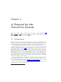
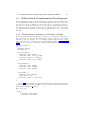
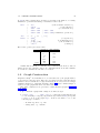
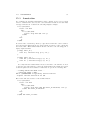
model transformation. Figure 1.1 depicts an architecture (the basic idea) of the
GRoundTram system. A model transformation is described in UnQL+, which is
functional (rather than rule-based as in many existing tools) and compositional
with high modularity for reuse and maintenance. The model transformation is
then desugared to a core graph algebra which consists of a set of constructors
for building graphs and a powerful structural recursion for manipulating graphs.
This graph algebra can have clear bidirectional semantics and be efficiently
evaluated in a bidirectional manner.
The note is intended to demonstrate, through a concrete example, how to
use the GRoundTram system to build a bidirectional transformation between
two models (graphs). The readers who are interested in the technical details
are referred to the technical papers (Hidaka et al. 2008, 2009a,b).
Note that all the sources discussed in this tutorial are available in the
examples directory in the distribution.
1
Pronounced [gráund træ̀m].
7
8
CHAPTER 1. A TUTORIAL FOR THE GROUNDTRAM SYSTEM
Figure 1.1: A Compositional Framework for Bidirectional Model Transformation
1.2
The Customer2Order Problem
As a concrete example, we consider the problem of developing a bidirectional
transformation between the customer model (customer graph) and the order
model (order graph), which is adapted from a similar example in the textbook
on model-driven software development (Pastor and Molina 2007).
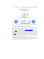
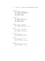
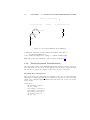
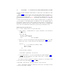
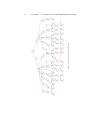
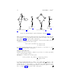
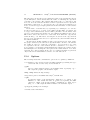
Figure 1.2 gives a simple graph representing customers’ information. The
graph has a root pointing to two customers, each having a name, some email
addresses, several addresses of different types (e.g. shipping or contractual customer address). A customer can have many customer orders. On the other hand,
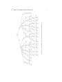
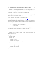
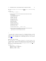
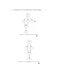
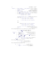
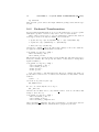
Figure 1.3 shows orders’ information, which actually corresponds to those orders
in the customers’ graph that are of type “shipping”. Each order contains order
information of the date, the order number, the customer name, and the address
to which the goods should be delivered.
We shall show how to construct a bidirectional transformation between these
two graphs such that changes on one graph can be propagated to the other one.
For example, if we change the ”BiG Office of Tokyo” to ”BIG Office at NII of
Tokyo” in either graph, we should propagate it to the other.
Figure 1.2: Cyclic Graph gcus Representing Customer-Centric Database
1.2. THE CUSTOMER2ORDER PROBLEM
9
Figure 1.3: Graph gord Representing Order-Centric Database
10
CHAPTER 1. A TUTORIAL FOR THE GROUNDTRAM SYSTEM
1.3. BIDIRECTIONAL TRANSFORMATION DEVELOPMENT
1.3
11
Bidirectional Transformation Development
The development consists of the following three big steps. An important feature
of the GRoundTram system is that if a transformation from one model to the
other is given, then updating of either model can be correctly propagated to
the other. So in the development of our bidirectional transformation between
the customer model and the order model, we will put effort into development
of a transformation mapping the customer graph (model) to the order graph
(model).
1.3.1
Representing Customers’ and Orders’ Graphs
To develop bidirectional transformation between two graphs (models), first of
all, we should be clear about the structures of the two graphs, i.e., the graph
schemas of the two graphs. For our running example, the structure of the
customer graph can be defined in the schema language KM3 (ATLAS group
2006). To be concrete, we build a file called Customer.km3 as follows.
package Customer {
datatype String;
datatype Int;
class Customer {
reference name: String;
reference email [1-*]: String;
reference add [1-*]: Address;
reference order [0-*]: Order;
}
class Address {
reference type: String;
reference code: String;
reference info: String;
}
class Order
reference
reference
reference
}
{
date: String;
no: Int;
order_of: Customer;
}
Figure 1.2 gives an instance graph that satisfies this structure. This instance
graph is clearly specified in UnCAL as follows. For later explanation, we save
it in the file customers c.uncal.
&src @ cycle(
(
&src :=
{ Customer: &customer1,
Customer: &customer2
12
CHAPTER 1. A TUTORIAL FOR THE GROUNDTRAM SYSTEM
},
&customer1 :=
{ name: {String: {"Tanaka"}},
email: {String: {"tanaka@biglab"}},
email: {String: {"tanaka@gmail"}},
add: {Address: &add1},
order: {Order: &order1},
order: {Order: &order2}
},
&customer2 :=
{ name: {String: {"Kato"}},
email: {String: {"kato@biglab"}},
add: {Address: &add1},
add: {Address: &add2},
order: {Order: &order3}
},
&add1 :=
{ type: {String: {"shipping"}},
code: {String: {"200-777"}},
info: {String: {"BiG office of Tokyo"}}
},
&add2 :=
{ type: {String: {"contractual"}},
code: {String: {"100-888"}},
info: {String: {"IPL of Tokyo"}}
},
&order1 :=
{ date: {String: {"16/07/2008"}},
no: {Int: {1001}},
order_of: {Customer: &customer1}
},
&order2 :=
{ date: {String: {"16/10/2008"}},
no: {Int: {1002}},
order_of: {Customer: &customer1}
},
&order3 :=
{ date: {String: {"16/12/2008"}},
no: {Int: {1003}},
order_of: {Customer: &customer2}
}
)
)
1.3. BIDIRECTIONAL TRANSFORMATION DEVELOPMENT
13
This is a rooted graph starting from the node &src, which points to two
customers. This UnCAL representation of a graph can be mapped to a graph
in the DOT format by the following command.
> uncalcmd -q customers_c.uncal -dot customers_c.dot
This will produce a dot file named customers c.dot, which can be viewed using
the standard graphviz system. For example, we can produce a graph in the
PNG format by the following command.
> dot customers_c.dot -T png -o customers_c.png
This will produce exactly the same graph as in Figure 1.2.
Given a (graph) schema and a graph, we can validate whether the graph satisfies the schema using the command unqlplus. For instance, we may validate
whether the graph customers c.uncal satisfies the schema Customers.km3 by
the following command.
> unqlplus -db customers_c.uncal \
-iv Customer.km3 -ip Customer \
-q c2o_c.unql
The last line specifies the transformation over the customers’ graph, which will
be developed later and is not important at this stage. One may create the
following simple identity transformation in the file c2o c.unql .
select $db
Similarly, we can specify the schema of the orders’ graphs (in the file
Order.km3) as follows.
package Order {
datatype String;
datatype Int;
class Order
reference
reference
reference
reference
}
{
no: Int;
date: String;
customer_name: String;
addr: Address;
class Address {
reference type: String;
reference code: String;
reference info: String;
}
}
14
CHAPTER 1. A TUTORIAL FOR THE GROUNDTRAM SYSTEM
1.3.2
Constructing Forward Transformation from Customer Model to Order Model
After formalizing the two graph schemas, we step to develop transformation from
the customer graph to the order graph. Suppose that this transformation is to
generate from the customers’ graph a graph that represents those information
of those orders that have type of “shipping”, such that its root points to all the
orders and each order contains order information of the date, the order number,
the customer name, and the address to which the goods should be delivered. We
can code this in UnQL+, our graph query/transformation language, as follows
(say in the file c2o c.unql).
select
{Order:
{date: $date,
no: $no,
customer_name: $name,
addr: {Address: $a}
}
}
where
{Customer.order.Order:$o} in $db,
{order_of.Customer:$c, date:$date, no:$no} in $o,
{add.Address:$a, name:$name} in $c,
{code:$code, info:$info, type.String:{$t:{}}} in $a,
$t = "shipping"
Now we can use the GRoundTram system to apply the transformation on the
customer graph customers c.uncal (that meets the schema Customer.km3)
to generate an order graph (say orders c.uncal) (that should meet the schema
Order.km3) by the command unqlplus.
> unqlplus \
-db customers_c.uncal \
-q c2o_c.unql \
-cal orders_c.uncal \
-iv Customer.km3 \
-ip Customer \
-ov Order.km3 \
-op Order
-t -pa -pu
This will produce an order graph in the file orders c.uncal, giving a bunch of
messages showing the intermediate results in the transformation: validating the
input graph, parsing the transformation (query), de-sugaring the transformation
to the internal core graph algebra in UnCAL, performing transformation, and
validating the output.
********* begin Input validation message *************
Input validation took 0.000345 CPU seconds
Validation succeeded.
VMap{Bid(0) => ‘klasse{kname = "Customer"}; Bid(3) => ‘datatype "Int";
Bid(6) => ‘datatype "String"; Bid(7) => ‘klasse{kname = "Customer"};
1.3. BIDIRECTIONAL TRANSFORMATION DEVELOPMENT
15
Bid(10) => ‘datatype "Int"; Bid(13) => ‘datatype "String";
Bid(14) => ‘klasse{kname = "Customer"}; Bid(17) => ‘datatype "Int";
Bid(20) => ‘datatype "String"; Bid(23) => ‘datatype "String";
Bid(26) => ‘datatype "String"; Bid(29) => ‘datatype "String";
Bid(32) => ‘datatype "String"; Bid(35) => ‘datatype "String";
Bid(38) => ‘datatype "String"; Bid(40) => ‘klasse{kname = "Order"};
Bid(42) => ‘klasse{kname = "Address"};
Bid(43) => ‘klasse{kname = "Address"}; Bid(46) => ‘datatype "String";
Bid(49) => ‘datatype "String"; Bid(51) => ‘klasse{kname = "Order"};
Bid(53) => ‘klasse{kname = "Order"}; Bid(55) => ‘klasse{kname = "Address"};
Bid(58) => ‘datatype "String"; Bid(61) => ‘datatype "String";
Bid(64) => ‘datatype "String"}
********** end Input validation message **************
(************** begin Submitted Query ****************)
select {Order:{date:$date, no:$no, customer_name:$name, addr:{Address:$a}}}
where
{Customer.order.Order:$o} in $db,
{order_of.Customer:$c, date:$date, no:$no} in $o,
{add.Address:$a, name:$name} in $c,
{code:$code, info:$info, type.String:{$t:{}}} in $a,
$t = "shipping"
(************** end Submitted Query ****************)
Desugaring took 0.000080 CPU seconds
(************** begin Executed UnCAL expr. ****************)
rec(\ ($L,$fv6).
if $L = Customer
then rec(\ ($L,$fv7).
if $L = order
then rec(\ ($L,$o).
if $L = Order
then rec(\ ($L,$fv5).
if $L = order_of
then rec(\ ($L,$c).
if $L = Customer
then rec(\ ($L,$date).
if $L = date
then rec(\ ($L,$no).
if $L = no
then rec(\ ($L,$fv4).
if $L = add
then rec(\ ($L,$a).
if $L = Address
then rec(\ ($L,$name).
if $L = name
then
rec(\ ($L,$code).
if
$L = code
then
rec(\ ($L,$info).
if
$L = info
then
rec(\ ($L,$fv1).
if
$L = type
then
16
CHAPTER 1. A TUTORIAL FOR THE GROUNDTRAM SYSTEM
rec(\ ($L,$fv2).
if
$L
= String
then
rec(\ ($t,$fv3).
if
$t
= "shipping"
then
{
Order:
{
date:
$date,
no: $no,
customer_name:
$name,
addr:
{
Address:
$a}}}
else
{})(
$fv2)
else
{})(
$fv1)
else
{})(
$a)
else
{})
($a)
else
{})
($a)
else
{})
($c)
else {})
($fv4)
else {})
($c)
else {})
($o)
else {})
($o)
else {})
($fv5)
else {})
($o)
else {})
($fv7)
else {})
($fv6)
else {})
1.3. BIDIRECTIONAL TRANSFORMATION DEVELOPMENT
17
($db)
(************** end Executed UnCAL expr. ****************)
Evaluation took 1.629894 CPU seconds
********* begin Output validation message *************
Output validation took 0.000101 CPU seconds
Validation succeeded.
VMap{Bid(2) => ‘datatype "Int"; Bid(5) => ‘datatype "String";
Bid(8) => ‘datatype "Int"; Bid(11) => ‘datatype "String";
Bid(14) => ‘datatype "Int"; Bid(17) => ‘datatype "String";
Bid(20) => ‘datatype "String"; Bid(23) => ‘datatype "String";
Bid(26) => ‘datatype "String"; Bid(29) => ‘datatype "String";
Bid(33) => ‘datatype "String"; Bid(35) => ‘klasse{kname = "Address"};
Bid(37) => ‘klasse{kname = "Address"};
Bid(39) => ‘klasse{kname = "Address"}}
********** end Output validation message **************
This finishes development of the (forward) transformation. Two remarks are
worth making. First, the command unqlplus is very powerful, with many useful
options; one can get information about the options of the command unqlplus
by typing
> unqlplus --help
Second, we can alternatively execute the following command to perform the
forward transformation which will produce more additional files (the ei file that
contains more editing information and the xg file that represents the result graph
being attached to the abstract syntax tree) that are necessary in the backward
transformation. Note that we omit graph validation here.
> fwd_uncal \
-db customers_c.uncal \
-uq c2o_c.unql \
-dot orders_c.dot \
-png orders_c.png \
-xg orders_c.xg \
-ei orders_c.ei \
-ge -pa
One can check the result graph by either seeing the graph in the PNG format
(i.e, orders c.png) or that in the DOT format (i.e., orders c.dot). Note that
this forward transformation command without validation is quite convenient and
useful, because it allows us to test transformation without giving the definition
of graph schemas.
1.3.3
Type Checking Forward Transformation
By specifying KM3 schemas via -iv and -ov options of the unqlplus command,
we can dynamically check at each run whether the given input graph and the
generated output graph meet the KM3 schemas.
In fact, the check can also be done statically. By passing input/output KM3
schema files and a transformation described either in UnQL+ or UnCAL to the
chkuncal command, we can verify that any graph satisfying the input schema
will always be transformed to an output graph satisfying the output schema.
In other words, once we have verified the correctness by chkuncal, we can be
18
CHAPTER 1. A TUTORIAL FOR THE GROUNDTRAM SYSTEM
sure that for all correct input graphs, the output graphs must meet the schema.
After the static checking, we can safely omit the per-run checking by -ov.
To use the typechecking facility of chkuncal, we need the MONA
tool (Project) to be installed on our system. Before trying the following examples, please download and set up MONA from http://www.brics.dk/mona/.
Static Type Checking Example
Consider we would like to check the correctness of the following transformation
c2date.uncal, which extracts all the shipping dates from the customer database
(the examples are placed in the example/typecheck directory):
rec( \($L,$G).
if $L =
else if $L =
else if $L =
else if $L =
else {}
)($db)
Customer then &
order then &
Order then &
date then {Date: {date: $G}}
Expected input graphs are those meeting the schema Customer.km3 used in
the previous section. But since for a technical reason the current version of
chkuncal does not accept the schema, we check the correctness against a slight
variant of the schema, Customer tc.km3:
package Customer_tc {
datatype String;
datatype Int;
class Customer {
reference name [0-*]: String;
reference email [0-*]: String;
reference add [0-*]: Address;
reference order [0-*]: Order;
}
class Address {
reference type[0-*]: String;
reference code[0-*]: String;
reference info[0-*]: String;
}
class Order {
reference date[0-*]: String;
reference no[0-*]: Int;
reference order_of[0-*]: Customer;
}
}
The difference is that we have added the number constraints [0-*] to all fields;
currently chkuncal can deal only with this type of schemas. The restriction
will be eliminated in a future version. For the detailed description of the subset
of languages supported by chkuncal, please consult Chapter 15.
Expected output graphs from c2date.uncal should be a collection of date
fields, capture by the following KM3 schema Date.km3:
1.3. BIDIRECTIONAL TRANSFORMATION DEVELOPMENT
19
package Date {
datatype String;
class Date {
reference date[0-*]: String;
}
}
To verify that the transformation is really correct with respect to the
schemas, what we need to type is the following one line of command:
> chkuncal Customer_tc.km3 c2date.uncal Date.km3
Then we will get the following diagnostics:
> chkuncal Customer_tc.km3 c2date.uncal Date.km3
...Loading Schema and UnCAL files...
...Converting UnCAL to MSO...
...Generating auxiliary formulas...
...Converting Schemas to MSO...
...Validation process is running (may take time)...
Success!
The message Success! means that the transformation is verified that it never
produces ill-typed outputs.
To see what happens if we try to verify a type-incorrect transformation, let
us consider another example, c2date-bad.uncal:
rec( \($L,$G).
if $L =
else if $L =
else if $L =
else if $L =
else {}
)($db)
Customer then &
order then &
Order then &
date then {Date: {data: $G}}
Can you see the difference? This version has a typo data (instead of date),
which makes the output not conforming to the schema. The chkuncal can
detect the badness as follows:
> chkuncal Customer_tc.km3 c2date-bad.uncal Date.km3
...Loading Schema and UnCAL files...
...Converting UnCAL to MSO...
...Generating auxiliary formulas...
...Converting Schemas to MSO...
...Validation process is running (may take time)...
Failure!
For a valid input
{Customer: {order: {Order: {date}}, order}, Customer},
the UnCAL program will produce an invalid output
{Date: {data}}.
When an error was found as above, chkuncal always exhibits a counter-example
(i.e., a graph that satisfies the input schema but yields an output graph not
satisfying the output schema) to help fixing the bug.
By using the -g option, the counter-example is exported in the .dot format
of the graphviz system.
20
CHAPTER 1. A TUTORIAL FOR THE GROUNDTRAM SYSTEM
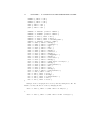
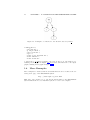
Chkuncal: a counter-example
A valid input tree
produces
an invalid output tree.
Customer Customer
order order
Date
data
Order
date
Figure 1.4: A Counter-Example from chkuncal
> chkuncal Customer_tc.km3 c2date-bad.uncal Date.km3 \
-g counter-example.dot
> dot counter-example.dot -Tpng -o counter-example.png
This will produce the visualized counter-example in Figure 1.4.
1.3.4
Testing Backward Transformation
One important feature of the GRoundTram system is that it can not only keep
trace information between the source (input) and the target (result) models,
but can also propagate the changes on the target model to the source.
Checking Trace Information
We can check the trace information by turning on the option -sb (set skolembulk) when executing the fwd uncal command so that the nodes of the result
graph can be attached with information showing where the nodes come in the
source graph.
> fwd_uncal \
-db customers_c.uncal \
-uq c2o_c.unql \
-dot orders_c_trace.dot \
-png orders_c_trace.png \
-xg orders_c_trace.xg \
-ei orders_c_trace.ei \
-sb -ge -pa
1.3. BIDIRECTIONAL TRANSFORMATION DEVELOPMENT
21
The generated graph is saved in the file orders c trace.dot. It has the following
contents.
digraph "g" {
node [ shape = "ellipse" ]
"FrE(FrE(FrE(FrE(FrE(FrE(FrE(FrE(FrE(FrE(FrE(FrE(FrE(FrE(FrE(
ImT (1047,&),
(37,\"shipping\",36),1051),
(38,String,37),1053),
(54,type,38),1055),
(54,info,32),1057),
(54,code,35),1059),
(66,name,64),1061),
(55,Address,54),1063),
(66,add,55),1065),
(52,no,17),1067),
(52,date,20),1069),
(14,Customer,66),1071),
(52,order_of,14),1073),
(53,Order,52),1075),
(66,order,53),1077),
(67,Customer,66),1079)"
[ label = "\N" ]
"FrE(FrE(FrE(FrE(FrE(FrE(FrE(FrE(FrE(FrE(FrE(FrE(FrE(FrE(FrE(
ImT (1047,&),(37,\"shipping\",36),1051),
(38,String,37),1053),(54,type,38),1055),
...
...
}
Here the name of each node is very long, containing information of all the
edges in the source graph that contribute to the construction of this node. For
example, the first node in the above example shows that it is related to the
edges such as (37,"shipping",36), (38,String,37) in the source graph in
Figure 1.2.
Editing the Order Graph
Before showing how to do backward computation to propagate changes on the
order graph to the original customer graph, let us see how to change the order
graph by editing. Since the order graph with trace information is long and
difficult to read, we shall work on the order graph in the file orders c.dot,
where all the nodes have simpler names.
digraph "g" {
node [ shape = "ellipse" ]
"n65658" [ label = "{&}\n\N" ]
"n65115" [ label = "\N" ]
"n65109" [ label = "\N" ]
22
CHAPTER 1. A TUTORIAL FOR THE GROUNDTRAM SYSTEM
"n44897" [ label = "\N"
"n44891" [ label = "\N"
"n44201" [ label = "\N"
"n44195" [ label = "\N"
"n64" [ label = "\N" ]
"n63" [ label = "\N" ]
"n62" [ label = "\N" ]
...
]
]
]
]
"n65658" -> "n65115" [ label = "Order" ]
"n65658" -> "n44897" [ label = "Order" ]
"n65658" -> "n44201" [ label = "Order" ]
"n65115" -> "n17" [ label = "no" ]
"n65115" -> "n20" [ label = "date" ]
"n65115" -> "n64" [ label = "customer_name" ]
"n65115" -> "n65109" [ label = "addr" ]
"n64" -> "n63" [ label = "String" ]
"n63" -> "n62" [ label = "\"Tanaka\"" ]
"n54" -> "n38" [ label = "type" ]
"n54" -> "n32" [ label = "info" ]
"n54" -> "n35" [ label = "code" ]
"n49" -> "n48" [ label = "String" ]
"n48" -> "n47" [ label = "\"Kato\"" ]
"n38" -> "n37" [ label = "String" ]
"n37" -> "n36" [ label = "\"shipping\"" ]
"n35" -> "n34" [ label = "String" ]
"n34" -> "n33" [ label = "\"200-777\"" ]
"n32" -> "n31" [ label = "String" ]
"n31" -> "n30" [ label = "\"BiG office of Tokyo\"" ]
"n20" -> "n19" [ label = "String" ]
"n19" -> "n18" [ label = "\"16/07/2008\"" ]
"n17" -> "n16" [ label = "Int" ]
"n16" -> "n15" [ label = "1001" ]
"n13" -> "n12" [ label = "String" ]
"n12" -> "n11" [ label = "\"16/10/2008\"" ]
"n10" -> "n9" [ label = "Int" ]
"n9" -> "n8" [ label = "1002" ]
"n6" -> "n5" [ label = "String" ]
"n5" -> "n4" [ label = "\"16/12/2008\"" ]
"n3" -> "n2" [ label = "Int" ]
"n2" -> "n1" [ label = "1003" ]
}
Changes on the order graph can be done by directly editing its dot file. For
instance, we may edit the above file by changing the line
"n31" -> "n30" [ label = "\"BiG office of Tokyo\"" ]
to
"n31" -> "n30" [ label = "\"BiG office at NII of Tokyo\"" ]
1.3. BIDIRECTIONAL TRANSFORMATION DEVELOPMENT
23
and save it to orders c mod.dot.
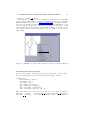
Alternatively, we may use our tool, Bdotty, a small extension of DOTTY
editor, for this editing. The tool should be installed easily if you already have
DOTTY installed. Please refer to Bdotty User’s Guide for installation instructions. Here we assume you have Bdotty command installed. With this tool, you
can, for example, edit the label of an edge by selecting “set edge label” on the
context menu that appears when it is called while pointing on the circle on the
edge. On the text box in the dialog window, type in “XXX” to set the label to
value “XXX”.
Figure 1.5: DOTTY screen shot while editing the result of a forward evaluation
Performing Backward Updating
Now we can propagate the changes on the target graph (the order model) to
the source graph (the customer model) with the following command.
> bwd_uncal \
-db customers_c.uncal \
-xg orders_c.xg \
-ei orders_c.ei \
-dot orders_c_mod.dot \
-png customers_c_mod.png \
-ucal customers_c_mod.uncal \
-udot customers_c_mod.dot -pa -cm
This will update the customer model and save the updated result in
different
formats
(customers c mod.png, customers c mod.uncal,
customers c mod.dot). Note that the current version of the system is
24
CHAPTER 1. A TUTORIAL FOR THE GROUNDTRAM SYSTEM
a bit slow in this backward transformation; it may take a few minutes for this
example.
Figure 1.11 shows the result of the backward transformation in which propagated modifications on edges or nodes are indicated by the following colors:
deleted parts are displayed in lightpink, added parts are displayed in purple, and
modified labels are displayed in red. Unreachable parts (if any) are displayed
in gray.
It is worth noting that the current backward transformation can fully support propagation of all valid in-place modification, but only partially support
propagation of insertion and deletion (that are independent of computation of
structural recursions). We treat complex insertion and deletion on graphs that
are produced by structural recursion in a special way, as discussed below.
Reflecting General Insertion
To be concrete, assume that we are given three files:
• a2d xc.uncal: a transformation to replace all labels a by d and short
edges labeled c.
rec(\ ($l,$g).
if $l = a then {d: &}
else if $l = c then &
else
{$l: &})($db)
• db.dot: a dot file representing the input graph (in Figure 1.6). Note that
this dot file can be obtained from the following uncal code (db.uncal)
cycle((
& := {a:{a:&z1},b:{a:&z1},c:&z2},
&z1:= {d:{}},
&z2:= {c:&z2}
))
by the following command.
> uncalcmd -q db.uncal -dot db.dot
• to be inserted.dot: a dot file representing the graph (in Figure 1.8) to
be inserted to the view later. Note this dot file can be obtained from an
uncal file, as seen above.
Note that by forward evaluation of a2d xc on db.dot, we can easily obtain
a view (view.dot) (as in Figure 1.7) by running
> uncalcmd -idot db.dot -q a2d_xc.uncal -odot view.dot
Now to demonstrate reflection of insertion on the view to the input, we may
execute the following command
1.3. BIDIRECTIONAL TRANSFORMATION DEVELOPMENT
Figure 1.6: An Input Graph for a2d xc
Figure 1.7: A View Graph Produced by a2d xc
25
26
CHAPTER 1. A TUTORIAL FOR THE GROUNDTRAM SYSTEM
Figure 1.8: A Graph to be Inserted to the View Produced by a2d xc
> bwdIg_uncal \
-idot db.dot \
-q a2d_xc.uncal \
-odot oview.dot \
-ipt 3 \
-tidot to_be_inserted.dot \
-uidot udb.dot \
-uodot uview.dot
to insert the to be inserted graph to the view at the node, say numbered 3,
resulting in the graph in Figure 1.9, and reflect this insertion to the input
graph, resulting in the graph in Figure 1.10.
1.4
More Examples
More examples for bidirectional model transformation can be found at the following demo page of the GRoundTram system.
http : //www.biglab.org/demo.html
This demo page enables one to test all the functionality of the GRoundTram
system without the need to install the system on one’s local computer.
1.4. MORE EXAMPLES
Figure 1.9: An Updated View
Figure 1.10: An Updated Input Graph
27
CHAPTER 1. A TUTORIAL FOR THE GROUNDTRAM SYSTEM
Figure 1.11: Updated Customers’ Graph
28
Part II
Language References
29
Chapter 2
UnQL+
UnQL+ is a high-level, SQL-like programming language for describing graph
transformations. UnQL+ extends the UnQL graph querying language (Buneman et al. 2000) with three simple graph editing constructs: replace, delete,
and extend.
2.1
Syntax
UnQL+ is a small extension of UnQL to support convenient specification of
graph transformations (model transformations). We extend UnQL with three
editing constructs for transforming graphs. An UnQL+ expression takes a graph
as input and results in a graph.
The following BNF defines the syntax of UnQL+ expr ession.
expr
::=
|
|
|
select template ( where bc1 , . . . , bcn )?
replace rpp ->gvar by template1 in template2
where bc1 , . . . , bcn
delete rpp ->gvar in template
where bc1 , . . . , bcn
extend rpp ->gvar with template1 in template2
where bc1 , . . . , bcn
The following BNF defines a graph.
31
(* selection *)
(* replacement *)
(* deletion *)
(* extension *)
CHAPTER 2. UNQL+
32
template
{label1 :template1 ,. . . ,labeln :templaten } (* union of graphs
template1 U template2
(* union of graphs
(* value of an expression
(expr)
fname(template)
(* function application
if bool cond then template1 else template2 (* conditional
(* variable binding
let gvar = template1 in template2
let sfun fname({lp1 :gp1 }) = template1
| fname({lp2 :gp2 }) = template2
...
| fname({lpn :gpn }) = templaten
in template
(* structural recursion
letrec sfun fname1 ({lp11 :gp11 }) = template11
| fname1 ({lp12 :gp12 }) = template12
...
| fname1 ({lp1m1 :gp1m1 }) = template1m1
and
...
and
sfun fnamen ({lpnm1 :gpnm1 }) = templatenm1
| fnamen ({lpn2 :gpn2 }) = templaten2
...
| fnamen ({lpnmn :gpnmn }) = templatenmn
in template
(* mutual structural recursion
gvar
(* graph variable
::=
|
|
|
|
|
|
|
|
The following BNF defines Boolean conditions and/or binding conditions.
bc
bool cond
::=
|
|
|
|
|
|
::=
|
bool cond (* boolean condition *)
bind cond (* binding condition *)
(bool cond)
(* parenthesized expression
isempty(template)
(* is the graph empty?
true | false
(* boolean literal
not bool cond | bool cond1 and bool cond2
bool cond1 or bool cond2
(* logical op
label1 = label2
label1 < label2 | label1 > label2 (* label comparison
bind cond
::=
gp in template (* binding condition *)
The following BNF defines label patterns.
lp
::=
|
lvar
(* label variable *)
rpp (* regular path pattern *)
The following BNF defines graph patterns.
gp
::=
|
|
gvar
(* graph variable *)
{lp1 :gp1 ,. . . ,lpn :gpn } (* union of graphs *)
const
(* constant *)
*)
*)
*)
*)
*)
*)
*)
*)
*)
*)
*)
*)
*)
*)
2.2. GRAPH QUERYING
33
The following BNF defines regular path patterns.
rpp
::=
|
|
|
|
|
|
label const
(* label
(* any label
rpp . rpp (* concatenation
(rpp | rpp)
(* union
rpp?
(* option
rpp+
(* one or more
rpp*
(* zero or more
*)
*)
*)
*)
*)
*)
*)
The following BNF defines label expressions.
label
::=
|
|
lvar
(* label variable *)
label const
(* constant *)
label ^ label (* concatenation *)
Var iables start with the $ sign. The label variables lvar and graph variables
gvar are not lexically distinguished.
letter
::=
a-z | A-Z | 0-9 |
|’
lvar
gvar
fname
::=
::=
::=
$letter∗
$letter∗
letter∗ (* function name *)
Operator precedence and associativity is:
(high)
(low)
2.2
2.2.1
Operator
not, isempty
*
.
|
^
=,<,>
and
or
U
,
Associativity
left
left
left
right
left
left
left
left
Graph Querying
The select-where Construct
A query of the form select template where bc1 ,. . . ,bcn extracts information
from graphs based on the binding and/or Boolean conditions bc1 , . . . , bcn
and constructs a graph according to the template.
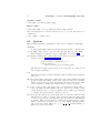
Example 1. The following query returns subgraphs that are pointed by b from
the root of $db.
select $G where {b : $G} in $db
CHAPTER 2. UNQL+
34
(b)
Result
(d)
of
Example 1
(a)
Input of Examples 1, 2 and
Result
of
Example 3
(c)
Result of Example 2
3
Figure 2.1: Result Graphs of Query Examples on Figure 2.1(a)
This query first matches the graph pattern {b : $G} against the graph $db and
gets bindings for $G, and then produces the result according to the select
part. Figure 2.1(b) shows the result of this query.
Example 2. The following query has multiple conditions in the where part and
construction of graphs in the select part.
select $G1 ∪ $G2 where {b : $G1 } in $db,
{a : $G2 } in $db
It returns all subgraphs that are pointed by either b or a from the root. Figure 2.1(c) shows the result of this query.
Regular Path Patterns
Regular path patterns, similar to XPath, are provided for concisely expressing
“deep” queries against a graph.
Example 3. Consider the following query.
select {result : $G1 } where { ∗.(a|b) : $G1 } in $db,
{$l : $G2 } in $G1 ,
$l 6= a
It extracts all subgraphs $G1 according to the regular path ∗.(a|b) (i.e., any
path ending with an edge labelled a or b), keeps those subgraphs that do not
contain an edge of a from their root, and glues the results with new edges
labelled result. It returns all subgraphs that are pointed by either b or a from
the root. Figure 2.1(d) shows the result of this query.
2.3. GRAPH EDITING
2.3
35
Graph Editing
UnQL+ is a small extension of UnQL to support convenient specification of
graph transformations (model transformations). We extend UnQL with three
editing constructs for transforming graphs: replace, delete and extend. For
graph editing, UnQL+ employs snapshot semantics, which is widely used in
many query languages such as SQL, XQuery!, XQueryU, Flux and so on. Snapshot semantics consists of two logical phases of processing: first, it specifies
nodes to be updated then updates are applied to the nodes. The semantics of
the graph editing is that for a given graph, starting from the root node of the
graph, it traverses every path and specifies nodes to be updated, then performs
editing on the nodes.
2.3.1
The replace-where Construct
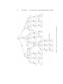
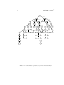
The replacement construct, replace ... where ..., is used to replace a subgraph by a new graph. For example, consider the Class graph in Figure 2.2,
how to prefix every name of the class by “class ” can be specified as follows.
Note that ”^” is a built-in function, which performs string concatenation.
replace _*.Class.name.String -> $u
by {("class_" ^ $name):{}} in $db
where {$name: $v} in $u
2.3.2
The delete-where Construct
The deletion construct, delete ... where ..., is used to describe deletion
of part of the graph. Consider the Class graph in Figure 2.2, how to delete all
persistent classes can be described by
delete Association.(src|dest).Class -> $class in $db
where {is_persistent.Boolean:true} in $class
where the subgraph matched with $class will be deleted from its original graph.
In contrast, the following transformation keeps the persistent classes as result.
select {result: $class}
where
{Association.(src|dest).Class: $class} in $db,
{is_persistent.Boolean:true} in $class
So, we may consider the delete as the dual of the select.
2.3.3
The extend-where Construct
The extension construct, extend ... where ..., is used to extend a graph
with another one. For example, we may write the following transformation to
add a date to each class.
extend _*.Class -> $u with {date:"2011/3/4"} in $db
CHAPTER 2. UNQL+
36
69
Association
Association
45
dest
44
50
Class
Attribute
19
type
17
name is_primary
22
PrimitiveDataType String
12
21
name
11
String
10
2
true
34
name attrs
48
64
String
String
"Phone"
"Address"
62
Boolean
Boolean
4
true
Class src_of
is_persistent
Attribute
true
3
String
25
"addr"
24
String
33
Boolean
false
type
37
name
15
"address"
68
Boolean
27
PrimitiveDataType
16
42
Attribute
38
18
56
attrs is_persistent name
39
23
26
57
53
is_primary name type
5
1
0
Class
32
63
name
65
46
59
58
Association
54
55
String
41
67
is_primary name
true
"Person"
8
40
66
Boolean
7
true
6
30
String
29
"name"
28
String
14
"Integer"
9
"number"
20
Boolean
35
src
51
Class src_of
"phone"
60
dest
61
49
attrs is_persistent name
36
52
Association
47
String
43
31
name src
"String"
13
Figure 2.2: A Class Model Represented by an Edge-Labelled Graph
Chapter 3
UnCAL
UnCAL is the core graph algebra of the graph query language UnQL (Buneman
et al. 2000) and our extension UnQL+ (see Chapter 2). Input and output graphs
for an UnQL+ program are written in the UnCAL format.
Moreover, UnCAL can also describe graph transformations, not just graphs
themselves. So, we have two graph transformation languages (UnQL+ and
UnCAL) in the GRoundTram system. Compared to UnQL+ , which is a more
high-level and user-friendly language, UnCAL is rather low-level and machinefriendly; indeed, in the GRoundTram system, all UnQL+ programs are first
compiled into UnCAL and then run. Although in most cases UnQL+ should
be sufficient for writing graph transformations, you can also write UnCAL programs directly. Besides, since the bidirectional transformation semantics of the
GRoundTram system is defined in terms of UnCAL, it might be helpful to know
the overview of UnCAL for understanding the bidirectional behavior.
We first show the full grammar of UnCAL in Section 3.1, and then, we give a
brief overview of each feature. For those who are interested only in how to write
input/output graph data by UnCAL, Section 3.2 is the important part. You
may skip other sections concerning graph transformations in Section 3.3. Note
that this manual is not intended to give a rigorous description of the UnCAL
language; the readers who are interested in the formal definition of the semantics
might want to consult the technical papers (Buneman et al. 2000; Hidaka et al.
2008, 2009a,b).
3.1
Syntax
The hole UnCAL program consists of one graph construction expr ession, defined
as in the following BNF. Compared to the original definition in (Buneman et al.
2000), the one implemented in the GRoundTram system adds two constructs let
and llet for ease of programming.
37
38
expr
CHAPTER 3. UNCAL
::=
|
|
|
|
|
|
|
|
|
|
|
|
|
|
|
|
{}
(* one-node graph
{ label1 : expr1 , . . . , labeln : exprn }
(* new node
expr1 U expr2
(* union
marker := expr (* label the root node with input marker
marker
(* graph with output marker
()
(* empty graph
expr1 ++ expr2
(* disjoint union
expr1 @ expr2
(* append
cycle( expr )
(* graph with cycles
(* same as expr1 ++ · · · ++exprn
(expr1 , . . . , exprn )
literal
(* same as {literal : {}}
gvar
(* variable reference
doc("char∗ ")
(* loading another file
if cond then expr1 else expr2
(* conditional
rec(\(lvar , gvar ) . expr1 )( expr2 ) (* structural recursion
let gvar = expr1 in expr2
(* variable binding
llet lvar = expr1 in expr2
(* label variable binding
*)
*)
*)
*)
*)
*)
*)
*)
*)
*)
*)
*)
*)
*)
*)
*)
*)
Operator precedence and associativity is:
(high)
(low)
Operator
@
if then else
U
:=
++
,
Associativity
left
right
left
right
left
Var iables start with the $ sign and mark ers start with the & sign. The label
variables lvar and graph variables gvar are not lexically distinguished.
letter
::=
a-z | A-Z | 0-9 |
lvar
gvar
marker
::=
::=
::=
$letter∗
$letter∗
(&letter∗)+
|’
Boolean cond itions are used as the branching condition for if expressions:
cond
::=
|
|
|
|
|
|
|
|
( cond )
(* parenthesized expression
isempty( expr )
(* is the graph empty?
isBool( label ) | isString( label )
isInt( label ) | isFloat( label )
isLabel( label )
(* type testing
true | false
(* boolean literal
not cond | cond1 and cond2 | cond1 or cond2 (* logical op
label1 = label2
label1 < label2 | label1 > label2
(* label comparison
*)
*)
*)
*)
*)
*)
3.2. GRAPH CONSTRUCTION
39
A label is either a (plain) label, an integer, a floating point number, or a string.
Arithmetic operations and string concatenation can be used:
label
char
literal
::=
|
|
|
|
lvar
literal
label ^ label
label + label
label * label
(* label variable reference
(* label literal
(* concatenation
| label - label
| label / label (* arithmetic operation
::=
::=
|
|
|
\" | \\ | [ ˆ"\]
letter+
[ 0-9] +
[ 0-9] + .[ 0-9] +
"char ∗ "
(* edge label
(* decimal integer
(* float number
(* string
*)
*)
*)
*)
*)
*)
*)
*)
Here is the operator precedence table:
(high)
(low)
Operator
*/
+- ^
<>
=
not
and
or
Associativity
left
left
left
left
left
UnCAL has two kinds of comments: line comments start from // and terminate at the end of the line, and block comments start from (* and terminate
at *). Block comments are allowed to be nested.
3.2
Graph Construction
Graphs in UnQL+ and UnCAL are rooted and directed cyclic graphs with no
order between outgoing edges. They are edge-labeled in the sense that all information is stored as labels on edges and the labels on nodes serve as a unique
identifier and have no particular meaning. Figure 3.1 gives a small example of
a directed cyclic graph with six nodes and seven edges.
Nine data constructors are provided to build arbitrary graphs (Buneman
et al. 2000).
• {}: constructs a graph with a single node without edges.
• { label1 : expr1 , . . . , labeln : exprn }: constructs a graph with the new
root node having n outgoing edges. Each edge is labeled labeli and points
to the root node of the graph expri . A label can either be one of the
following type of values:
– Normal edge label, e.g., abc.
– String value, e.g., "world".
40
CHAPTER 3. UNCAL
Figure 3.1: A Simple Graph
– Integer value, e.g., 42.
– Floating point value, e.g., 3.14.
Data-valued edges, i.e., edges labeled with string, integer, or floating point
values, must point to a node with no further outgoing edges. For these
edges, destination expr can be omitted; {"world", 42} is equivalent to
{"world": {}, 42: {}}.
• expr1 U expr2 : unifies two graphs by creating a new root and connect it to
the roots of expr1 and expr2 using ε-edges. An ε-edge is used to represent
a shortcut of two nodes, and works like ε-transition in automaton. For
instance, {a:100} U {b:200} is defined to be the graph {ε:{a:100},
ε:{b:200}}, which is equivalent to {a:100, b:200}.
• &x := expr: adds an input marker &x to the root of expr. A node marked
with an input marker is sometimes called an input node. Intuitively, input
nodes can be regarded as root nodes of the graph fragment. For singly
rooted graphs, we implicitly use the default marker & to indicate its single
root.
• &y: constructs a graph with a single node, which is marked with an output
marker &y. Such a node is called an output node. An output node can
be regarded as a “context-hole” of graphs where an input node with the
same marker is plugged later.
• (): constructs an empty graph which has neither a node nor an edge.
• expr1 ++ expr2 : constructs the disjoint union of two graphs. Two graphs
are simply juxtaposed and no connecting edges (like ε-edges of the U operator) are added. A syntactic sugar (expr1 , · · ·, exprn ) stands for expr1
++ · · · ++ exprn .
• expr1 @ expr2 : appends two graphs. The resulting graph is obtained by
plugging the input nodes of expr2 into their corresponding output nodes
in expr1 .
3.3. GRAPH TRANSFORMATION
41
• cycle( expr ): connects the input nodes with the output nodes of expr to
form cycles.
As an instance, the graph in Figure 3.1 can be expressed in the following
UnCAL expression:
&root @ cycle(
(
&root := {a: {a: &5}, b: {a:&5}, c: &4},
&5 := {d: {}},
&4 := {c: &4}
)
)
3.3
3.3.1
Graph Transformation
Structural Recursion
In addition to the graph constructors, structural recursion is essential for writing
graph transformations.
expr
::=
|
|
···
rec(\(lvar , gvar ) . expr1 )( expr2 ) (* structural recursion *)
···
Structural recursion has two equivalent semantics under the graph bisimulation: bulk semantics and recursive semantics. The former is the prominent feature of structural recursion, whereas the latter is the usual recursive semantics
with memoization. Informally, the bulk semantics for the expression rec(\($L,
$G) . expr1 )( expr2 ) is that the function \($L, $G) . expr1 (backslash should
be read as λ of the lambda-calculus) is applied independently on all edges of
graph expr2 , then the results are joined together with ε-edges (as in the @ operation). At each edge, the label of the edge is bound to the label variable $L and
the graph rooted from the destination node of the edge is bound to the variable
$G. For instance,
&z @ rec(\($L,$G).
if $L = a then
&z := {b: &z}
else if $L = c then
&z := {c: $G}
else
&z := {$L: &z}
)($db)
this recursion replaces each edge labeled a by a graph &z:={b:&z}, edge labeled
c by {c:$G} where $G is the destination node of the original edge, and other
edges labeled $L are replaced by &z:={$L:&z}. Those graph fragments are glued
together by the &z marker. In effect, we obtain a graph whose a-edges (except
the ones under c-edges) are replaced by b-edges.
42
3.3.2
CHAPTER 3. UNCAL
Input and Output Graphs of Transformations
The input graph of a transformation is given to an UnCAL program as the
global variable $db, which is specified by the -db or the -dbd option of the
uncalcmd command (see Chapter 8). Additionally, by using the doc(filename)
expression, a graph is read from the UnCAL file filename. The name of the file
must be supplied by a string literal: e.g., "my-database.uncal". Dynamically
computed string values cannot be used there.
The output graph of the transformation is the result obtained by evaluating
the whole expression.
Chapter 4
KM3
The GRoundTram system validates input and output graphs against given
schemata of them. We employ the Kernel MetaMetaModel (KM3) (ATLAS
group 2006) to describe schemata. KM3 is an architecture-neutral language to
write metamodels, which was developed at INRIA and is supported under the
Eclipse platform. KM3 is structurally close to EMOF 2.0 and Ecore, but much
simpler. We refer to a metamodel written in KM3 notation as KM3 schema.
4.1
Syntax
A KM3 schema has a structure similar to an XML schema based on regular
tree grammars such as W3C XML schema (W3C XML Schema WG) in the
sense that a schema prescribes which kind of set of nodes must be referred to
by a node by regular expression. Figure 4.1 gives the definition of the core of
KM3. The difference from the original definition (ATLAS group 2006) is that
the enumeration class is not supported in our system. Note that validation
with regard to ordered references and multiplicities of features does not make
sense in the context of UnQL/UnCAL graph models where bisimilar graphs are
treated as the same. There are two bisimilar graphs, one has only one child at
the root node and another has two. For a similar reason, we cannot deal with
oppositeOf relationships (ATLAS group 2006) between two classes in UnCAL
graphs.
We will not explain the details of KM3. Instead we explain KM3 informally
with an example.
A KM3 schema is a set of packages which consists of classes, data types and
enumerations. Figure 4.2 shows an example of a KM3 schema for a simplified
UML Class specification. The schema consists of four classes, Association,
Class, Attribute and PrimitiveDataType. A class has some features, either
references or attributes. Every feature has a type, either class or data type.
Since all of them inherit from their super class NamedElt, they have an attribute
name which is of type String. The Association class has two references src and
dest which are of type Class. The Class class has an attribute is persistent
which is Boolean and an arbitrary number of references attrs which are of type
Attribute. The Attribute class has an attribute is primary which is Boolean
43
44
CHAPTER 4. KM3
package
classifier
feature
multiplicity
::=
::=
|
::=
|
::=
|
package name { ( classifier )∗ }
(* package
(abstract)? class name
(extends name(, name)∗ )? { ( feature )∗ } (* class
datatype name ;
(* primitive datatype
attribute name ( multiplicity )? : name ; (* attribute
reference name ( multiplicity )? : name ; (* reference
[ number - number ]
(* with lower and upper bound
[ (number -)? * ]
(* with lower bound
Figure 4.1: KM3 Syntax
and a reference type which is a PrimitiveDataType. The PrimitiveDataType
class has neither an attribute nor a reference besides the inherited attribute
name.
4.2
Validation
We validate a graph by matching each contained edge with a name of a class or
a feature in a given schema. A validation of a graph proceeds as follows.
1. All class inheritances are eliminated from a given schema by expanding
features of classes with their super classes. The elimination is recursively
done since a super class may inherit another super class.
2. We associate a vertex following from the root of the graph with a class
whose name is the same as the label of the edge between the vertex and
the root.
3. We match a set of labels on edges from the vertex with a set of names
of features of the class. Every destination vertex of the edge should have
edges which are labelled by the name of a class or a data type of the
feature and the number of which is specified by a multiplicity in the KM3
schema such as [*] in Figure 4.2. If the label of the edge is the name of
the class, the destination vertex of the edge is associated with the class
and is checked the feature again. If the label of the edge is the name of the
data type, the destination vertex of the edge should have an edge whose
label has the same type and whose destination vertex has no edge. This
step is repeatedly performed until all vertices in the graph are visited.
This procedure always terminates because the number of vertices are finite.
*)
*)
*)
*)
*)
*)
*)
4.2. VALIDATION
package Class {
datatype String;
datatype Boolean;
abstract class NamedElt {
attribute name : String;
}
class Association extends NamedElt {
reference src : Class;
reference dest : Class;
}
class Class extends NamedElt {
attribute is_persistent : Boolean;
reference attrs [*] : Attribute;
}
class Attribute extends NamedElt {
attribute is_primary : Boolean;
reference type : PrimitiveDataType;
}
class PrimitiveDataType extends NamedElt {
}
}
Figure 4.2: KM3 Schema for UML Classes
45
46
CHAPTER 4. KM3
Part III
Command References
47
Chapter 5
GRoundTram Main
Command (gtram)
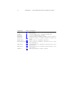
This chapter describes the main command that invokes subcommands. They
are described in the following chapters.
5.1
Overview of the Main Command
This command invokes each subcommand with their respective arguments. The
following command line
> gtram fwdI_uncal -- -db db.dot -q trans.uncal -png result.png \
-dot result.dot
invokes command fwd uncal described in chapter 9. Note that the arguments
for the subcommand should follow a double hyphen (“–’). The commands that
can be invoked are summarized in Table 5.1. Each command should be executable by having its inhabiting directory included in the user’s command
search paths.
5.2
Options
The following additional command-line options are recognized by gtram.
-d Prints debugging information.
-help
Displays list of options.
49
50
command
unqlplus
CHAPTER 5. GROUNDTRAM MAIN COMMAND (GTRAM)
chap. description
6
execute UnQL+ transformation/validate graph against
KM3 schema.
desugar
7
converts UnQL+ file to equivalent UnCAL files.
8
execute UnCAL unidirectionally.
uncalcmd
fwd_uncal
9
foward execution of UnQL+/UnCAL for in-place updates.
bwd_uncal
10
backward execution of UnQL+/UnCAL for in-place updates.
bwdIg_uncal
11
bidir. execution of UnCAL for insertions.
bwdI_enum_uncal 12
bidir. execution of UnCAL for insertions based on candidate enumeration.
fwdI_uncal
13
forward execution of UnCAL for insertions based on insertion units.
bwdI_uncal
14
backward execution of UnCAL for insertions based on insertion units.
chkuncal
15
static typechecking of UnQL+/UnCAL.
Chapter 6
UnQL+ Interpreter
(unqlplus)
This chapter describes the UnQL+ interpreter unqlplus, which interprets
UnQL+ source files for input graphs and produces output graphs in various
formats.
6.1
Overview of the Interpreter
This command evaluates UnQL+ queries on a specified input graph by translating the UnQL+ to UnCAL graph algebra and then interpret the algebra to
produce an output graph. Output formats can be DOT for Graphviz package,
UnCAL, and other image formats supported by the Graphviz package. It can
optionally validate input and output graphs when a KM3 schema is specified.
The command line
> unqlplus -db src.uncal -q trans.unql -png result.png
loads an input graph specified by file src.uncal and binds to variable $db, interprets UnQL+ source trans.unql, and saves the result graph to result.png.
Option -db is mandatory.
Multiple input may be specified using -var options as described in the next
section.
If you just want to verify a graph, -q option is not necessary – just specify
-iv and -ip options like
> unqlplus -db src.uncal -iv Class.km3 -ip Class
6.2
Options
The following additional command-line options are recognized by unqlplus.
-v Prints version information.
51
CHAPTER 6. UNQL+ INTERPRETER (UNQLPLUS)
52
-oi file
Saves the image of result graph to file. Format of the image is specified by
the extension of the filename. Supported formats are the same as those
supported by -T option of dot command in Graphviz.
-png file
Saves PNG image of result graph to file.
-dot file
Saves result graph in DOT format to file.
-cal file
Saves result graph in UnCAL format to file.
-var v =file
Binds a graph in UnCAL format specified by file to variable $v . Multiple
variables can be bound by repeatedly using this option.
-iv file -ip package
Validates the input graph specified by -db option using KM3 schema package package defined in file. If validation succeeds, a map of known classifiers which maps a node number to the name of feature associated with
the node is printed. BNF for the output syntax is as follows.
Result
entry
classifier
node
::=
::=
::=
|
::=
VMap{ entry ( ; entry )* }
node => classifier
‘datatype string
‘klasse { kname = string }
Node ID in the UnCAL graph data model
For example, the output
Bid(2) => ‘datatype "Boolean";
Bid(32) => ‘klasse{kname = "Attribute"}
denotes that the node No. 2 is detected to have a primitive data type
“Boolean”, and node No. 32 belongs to a class named “Attribute”.
-ov file -op package
Validates the output graph using KM3 schema package package defined
in file. Output format is identical to that of -ov and -op option.
-bulk
Bulk semantics is used for the interpretation of UnCAL structural recursion rec. Recursive semantics is used without this option.
-t Prints elapsed user (CPU) time broken down to
•
•
•
•
input validation (if -iv and -ip options are specified)
desugaring
execution of UnCAL expression
output validation (if -ov and -op options are specified)
6.2. OPTIONS
53
-oa Optimizes evaluation of @ and equivalent operation in evaluation of rec
when recursive semantics (default) is used. @ usually evaluates both
operands and connects matching I/O nodes. However, if an I/O node
does not match, the second operand is left unconnected and made unreachable. This option suppresses the evaluation of the second operand
to save evaluation time. In case of recursive semantics that is based on
primary definition of structural recursion
f {l : t} = e(l, t) @ f (t),
it suppress recursion to f (t) if e(l, t) produces no output marker, i.e., f is
essentially non-recursive.
-ea Applies Skolem term to each node of the graph generated by the first
operand of @. Users usually do not have to specify this option. See
Description of bidirectional UnQL+/UnCAL demonstration for more information.
-pa Prints UnCAL expression after desugaring.
-pu Prints UnQL expression before desugaring.
-m Produces unique name for each marker in the body of rec. Desugaring
module usually reuses marker symbols for different rec bodies. However,
when results of two different rec are unified using operators such as U,
undesired node sharing may result. This form of UnCAL may be produced
from an UnQL expression of the form select ... U select. This option
suppresses this sharing by using different set of markers for different rec.
This sharing can be avoided using -pi option as well. Non-recursive rec
also uses explicit markers when this option is specified. For example,
rec(λ(l, t).{l : t})($db)
becomes
&z1 @ rec(λ(l, t).&z1 := {l : t})($db)
-sr Uses Skolem term (S1 in (Buneman et al. 2000)) in the evaluation of rec
using recursive semantics. Straightforward interpretation of recursive semantics would not use Skolem term that is usually used for bulk semantics,
but undesired sharing might result when transformation is in a specific
form described in -m option section without this option.
-pi Uses node id based on lexical position of node construction expression.
Without this option, new node id is generated for each evaluation even
if node construction expression is lexically identical. This option makes
expressions referentially transparent albeit with more complicated node
IDs that may make visualized graph nodes larger.
-pn Prefixes output base node number with “n”. This is an alignment to the
node id format produced by DOTTY (and our variant of it BDOTTY).
This option is necessary if you edit output DOT file with these editors.
CHAPTER 6. UNQL+ INTERPRETER (UNQLPLUS)
54
-cg Contracts the output graphs to their normal form based on bisimulation
equivalence1 . After contraction, no two nodes are bisimilar to each other.
In particular, leaf nodes (nodes that has no outgoing edges) are bisimilar
to each other, so they all shrink to one node.
Since UnQL (and UnCAL) is based on bisimulation, transformation may
introduce redundant nodes that are bisimilar to each other. This option
is useful when such redundancy has to be eliminated.
Note that the normal forms obtained may have different node ID assignments — although they are isomorphic to each other — even if they are
generated from bisimilar graphs. Since Graphviz which we use as our
graph layout tool depends on the ID, the difference may result in a different layout.
-ht Turns on holistic transitive closure (TC) computation optimization in rec
for both bulk and recursive semantics.
rec(λ(l, t).e)($db) requires computation of TC for every node in the graph
bound to $db. By default, this TC is computed on per-node basis. -ht
option let the interpreter compute the TC at once, enabling the reuse of
TC for a node to compute TC of the nodes in the vicinity of the former
node.
However, since default TC computation is already efficient for a small number of nodes because it performs one depth-first search only using index
from node to outgoing edges, this option may cause a performance slowdown. It performs better only when the input graph has large stronglyconnected components2 (i.e., many of the nodes in the graph are connected
to each other either directly or indirectly) and query visits most of the
nodes.
-help
Displays list of options.
1 The
partition refinement alogithm by Paige and Tarjan (Paige and Tarjan 1987) is used.
by Tarjan’s algorithm(Tarjan 1972)
2 Captured
Chapter 7
UnQL+ to UnCAL
Compiler (desugar)
This chapter describes UnQL+ compiler desugar, which converts UnQL+ source
files to equivalent UnCAL file.
7.1
Overview of the Compiler
The command line
> desugar trans.unql
translates an UnQL+ source file trans.unql to UnCAL and prints it to standard
output.
7.2
Options
The following additional command-line options are recognized by desugar.
-v and -m
The meanings are identical to those of unqlplus. See section 6.2.
55
56
CHAPTER 7. UNQL+ TO UNCAL COMPILER (DESUGAR)
Chapter 8
UnCAL Interpreter
(uncalcmd)
This chapter describes UnCAL interpreter uncalcmd, which interprets UnCAL
source files for input graphs and produces output graphs in various formats.
8.1
Overview of the Interpreter
This command evaluates an UnCAL query on specified input graph and produces an output graph.
The command line
> uncalcmd -db db.uncal -q trans.uncal -png result.png
loads input graph specified by file src.uncal and binds to variable $db, interprets UnCAL source trans.uncal, and saves the result graph to result.png.
The option -q is mandatory.
It can also be used to perform conversion between DOT and UnCAL formats
as follows.
UnCAL to DOT
> uncalcmd -q a.uncal -dot a.dot
converts UnCAL file a.uncal to DOT file a.dot.
DOT to UnCAL
> uncalcmd -dbd a.dot -q identity.uncal -cal a.uncal
converts DOT file a.dot to UnCAL file a.uncal, where identity.uncal is a text
file that only contains $db that represents identity transformation.
If you want to generate a PNG from UnCAL file or DOT file, do the following.
57
58
CHAPTER 8. UNCAL INTERPRETER (UNCALCMD)
UnCAL to PNG
> uncalcmd -q a.uncal -png a.png
DOT to PNG
> uncalcmd -dbd a.dot -q identity.uncal -png a.uncal
where identity.uncal is a text file described above, or you can directly use dot
command by
> dot -Tpng -o a.png a.dot
8.2
Options
The following additional command-line options are recognized by uncalcmd.
-dbd file
Loads a graph DOT format specified by file and binds it to variable $db.
-v, -oi, -png, -dot, -cal, -t, -oa, -ea, -pa, -sr, -pi, -pn, -cg, -ht, -help
The meanings are identical to those of unqlplus. See section 6.2.
-rw Applies rewriting rules. This includes fusion rules of two successive applications of rec in (Buneman et al. 2000):
rec(e2 ) ◦ rec(e1 ) = rec(rec(e2 )) ◦ e1
rec(e2 ) ◦ rec(e1 ) =
rec(λ(l, t). rec(e2 )(e1 (l, t) @ rec(e1 )(t)))
The first rule is applied when e2 (l, t) does not depend on t. The second
rule is applied otherwise.
-rec
Interprets rec using recursive semantics. Bulk semantics is used without
this option.
-lu Leaves unreachable parts in the result graph. Since bulk semantics typically
produces many unreachable parts, these parts are removed by default.
Other operators that produces unreachable parts are cycle and @. This
option is useful to examine the formal behavior of these operators.
-le Leaves ε-edges in the result graph. Since rec typically produces many εedges especially in bulk semantics, they are removed by default. Other
operators that produces ε-edges are cycle, @ and ∪. This option is useful
to examine the formal behavior of these operators.
-ls Leaves Skolem terms in the result graph. Since rec produces Skolem terms
which nests according to nesting of rec, and may make the result graph
too large to perceive the entire structure, they are renamed to flat numbers
by default. This option is useful to examine the formal behavior of rec.
Other operators are extended by us to produce similar structured IDs if
-pi option is specified. These are ∪, {}, { : }, & (output marker), @
(with -ea option), and cycle.
8.2. OPTIONS
59
-pr Prints UnCAL expression that is actually evaluated. This is useful to examine the expression after rewriting. This is identical to the expression
printed by -pa option if -rw option is not specified.
-rc Renders record shape nodes using node attribute record in DOT format
of Graphviz. Default is ellipse. This option is useful when you edit
the DOT format file produced by -dot option using DOTTY instead of
BDOTTY. Please refer to Description of bidirectional UnQL+/UnCAL
demonstration for the usage of record mode.
60
CHAPTER 8. UNCAL INTERPRETER (UNCALCMD)
Chapter 9
UnQL+/UnCAL Forward
Interpreter (fwd uncal)
This chapter describes the forward transformation part of bidirectional
UnQL+ /UnCAL interpreter fwd uncal, which interprets UnQL+ /UnCAL
source files for input graphs and produces an output graph with trace
information for backward evaluation. This command is intended to be used
with bwd uncal described in chapter 10.
9.1
Overview of the Forward Interpreter
This command evaluates UnQL+ /UnCAL queries on a specified input graph
and produces an output graph with trace information.
The command line
> fwd_uncal -db src.uncal -uq trans.unql -png result.png \
-dot result.dot -xg result.xg -ei bd.ei
loads an input graph specified by file src.uncal1 and binds to variable $db,
interprets UnQL+ source trans.unql, and saves the executed UnCAL expression augmented with result graph to result.xg. It also saves the result
graph to DOT file result.dot for editing and further backward evaluation
with bwd uncal. Various evaluation information is also stored in bd.ei. These
files, together with source graph src.uncal should be passed to bwd uncal
when backward evaluation is necessary. Options -db, -dot, -xg and -ei are
mandatory. As for transformation, either -uq (UnQL+ query) or -q (UnCAL
query) should be specified. The image of the result graph stored in result.png
is just for preview and not required for backward evaluation.
Unlike the unidirectional evaluator uncalcmd, bulk semantics is always used
for traceability.
1 DOT
file can be accepted as well.
61
62CHAPTER 9. UNQL+ /UNCAL FORWARD INTERPRETER (FWD UNCAL)
9.2
Options
The following additional command-line options are recognized by fwd uncal.
-q file
Evaluates an UnCAL query specified by file instead of UnQL+ .
-v, -pa, -rw, -su, -ea
The meanings are identical to those of uncalcmd. See section 8.2.
-ge Glues source node and target node of each ε-edge and removes that edge if
it is safe to do so. In general, if the source of an ε-edge is an input node or
has other outgoing edges, and the target of the ε-edge has other incoming
edges, gluing would introduce a spurious path that is inexistent before
the gluing, so gluing does not take place. Another source of danger is the
ambiguity of correspondences between graphs before and after gluing. If
the two edges end up with sharing their source and target as a result of
gluing, and users edit either of both of the edges, it is difficult to determine
to which edge before gluing the editing effect should be propagated. In this
situation, this option is ignored and gluing does not take place. Specifying
this option produces a simple graph which is easy to edit, while unchecking
helps understanding of the forward semantics of the constructors.
Since rendering a large graph is time-consuming (it may take several minutes), when you execute a query that is expected to produce a large graph
if gluing would not be applied, this option is recommended.
-sb Uses Skolem terms which are constructors that enables rendezvous
between connected subgraphs.
For example, bulk semantics uses
Hub(nodeid , marker , exprid ) 4 where expid identifies subexpression,
and nodeid itself is a node ID. Bulk semantics generates nodes and
edges independently from each input node and edge. Connecting these
components are possible thanks to the Skolem terms. While edges (n1,
l1, n2) and (n3, l2, n4) can be connected via node IDs n5 if n2, n3 and
n5 coincide, the Skolem terms generated by rec and other constructors
enable this coincident.
-to time
Sets timeout to time seconds. Evaluation is aborted after this time period.
The bidirectional evaluator takes more time than unidirectional evaluators
due to maintenance of trace information. This option is useful for batch
processing in which a long-running execution is undesirable.
-cs Use simplified semantics for cycle in which only mismatched marker remains. Default semantics leaves every input node regardless of combination of I/O nodes in the operand.
-np Do not prefix output base node number with “n”. This flag is just the
opposite effect of -pn in unqlplus and uncalcmd. Since our current editor is DOTTY (and our variant of it BDOTTY), the default behavior is
prefixing to align with these tools.
-t Prints elapsed user (CPU) time broken down to
9.2. OPTIONS
• rewriting (if -rw option is specified)
• forward execution of UnCAL expression
63
64CHAPTER 9. UNQL+ /UNCAL FORWARD INTERPRETER (FWD UNCAL)
Chapter 10
UnCAL Backward
Interpreter (bwd uncal)
This chapter describes the backward transformation part of bidirectional
UnQL+ /UnCAL interpreter bwd uncal, which interprets UnQL+ /UnCAL
source files for modified output graphs and produces input graph in which
modification on the output graph is reflected. Note that this propagation does
not always succeed. This command is intended to be used with fwd uncal
described in chapter 9.
10.1
Overview of the Backward Interpreter
This command evaluates an UnQL+ /UnCAL query on specified output graph
along with trace information and produces an input graph with modification on
the output graph being reflected.
The command line
> bwd_uncal -db src.uncal -xg result.xg -ei bd.ei \
-dot result.dot -ucal srcprime.uncal -png srcprime.png
loads an input graph specified by file src.uncal1 and binds to variable $db,
interprets UnQL+ /UnCAL source backwards using evaluation mode that had
been saved in result.xg and result.ei by the fwd uncal command, and saves
updated source graph to srcprime.uncal in UnCAL format. It also saves the
image of the updated source graph in srcprime.png for preview. Options -db,
-xg, -ei and -dot are mandatory.
10.2
Options
The following additional command-line options are recognized by bwd uncal.
-v Prints version information.
1 DOT
file can be accepted as well.
65
66
CHAPTER 10. UNCAL BACKWARD INTERPRETER (BWD UNCAL)
-udot file
Saves updated source graph to file in DOT format.
-pa Prints UnCAL input expression saved in file specified by -xg option.
-cm Colors modification to source DB specified by -png. Modifications propagated by the backward transformation are indicated by the color of edges
or nodes: deleted parts are displayed in lightpink, added parts are displayed in purple, and modified labels are displayed in red. Unreachable
parts (if any) are displayed in gray.
-np Do not prefix node number in the update source DB specified by -png or
-udot DB with “n”. See also the same option of fwd uncal described in
chapter 9.
-t Prints elapsed user (CPU) time for the backward execution of the UnCAL
expression.
Chapter 11
UnCAL Backward
Interpreter with Insertion
of Graph (bwdIg uncal)
11.1
Overview of the UnCAL Backward Interpreter for Insertion of Graph
This command performs the reflection of insertion of a graph on the target back
to the source graph. It is implemented in a completely different manner than
command bwdI uncal in chapter 14, and provides a more intuitive interface.
This command is used in the following steps:
1. Forward execution.
> bwdIg_uncal -idot db.dot -q q.uncal -odot output.dot \
[-opng result.png]
loads input graph specified by file db.dot and binds to variable $db, interprets UnCAL source q.uncal, and save the output target graph in file
output.dot. It optionally saves the PNG file of the output in result.png
if it is specified. Options -idot, -q and -odot are mandatory.
2. User determines the insertion point in terms of the ID of the node on the
target graph by examining output.dot or result.png. Let’s assume here
that the node number 1 is selected.
3. User determines the graph to be inserted and prepare it as a dot file. Let’s
assume here that it is saved in tidot.dot.
4. Reflection of insertion to the input graph.
> bwdIg_uncal -idot db.dot -q q.uncal -odot output.dot \
-ipt 1 -tidot tidot.dot -uidot udb.dot -uodot uoutput.dot
67
68
CHAPTER 11. BWD. INTERP. WITH INSERTION (BWDIG UNCAL)
executes the query q.uncal in “insertion mode”, and reflects the insertion
of the graph tidot.dot at the target graph output.dot rooted at node
id 1, and saves the new input graph to udb.dot as well as a new target
graph to uoutput.dot. In this step, options -ipt, -tidot, -uidot and
-uodot are mandatory. The other options (and content of the files) should
be exactly identical to those specified in the first step.
Note that this step does not always succeed. For example, if the result
graph of insertion on the target side (i.e., to be saved in uoutput.dot
in the above command line) is not within the range of the transformation
(specified by q.uncal), then the insertion is inherently impossible, because
no matter what graph you give as an input, the new target graph can never
be generated by the transformation.
In case of this failure, you either get the error message ”no insertion exists on the source side”, or the command does not return (i.e., does not
terminate).
Also note that if you insert a large graph, then this step may take a long
time.
11.2
Options
The following additional command-line options are recognized by bwdIg uncal.
-pa
Prints the UnCAL expression given by -q option.
Chapter 12
UnCAL Backward
Interpreter with Insertion
of Graph (bwdI enum uncal)
12.1
Overview of the UnCAL Backward Interpreter for Insertion of Graph based on
Enumeration
This command performs the reflection of insertion of a graph on the target back
to the source graph. It provides more direct access to the implementation of the
command bwdIg uncal in chapter 11. bwdI enum uncal works on the view that
reveals trace information in their node IDs, epsilon edges, and requires selection
of a graph to be inserted from the candidates enumerated by the implementation.
This command is used in the following steps:
1. Forward execution.
> bwdI_enum_uncal -idot db.dot -q q.uncal -odot output.dot \
[-opng result.png]
loads an input graph specified by file db.dot and and binds to variable
$db, interprets UnCAL source q.uncal, and saves the output target graph
in file output.dot. It optionally saves the PNG file of the output in
result.png if it is specified. Options -idot, -q and -odot are mandatory.
Note that unlike bwdIg uncal, the target graph saved in output.dot reveals the raw internal representation which includes trace ID of the nodes
and epsilon edges.
2. The user determines the insertion point in terms of the ID of the node on
the target graph by examining output.dot or result.png. Let’s assume
here that the node Hub(2,&,9) is selected. The node ID enriched with
69
70CHAPTER 12. BWD. INTERPRETER WITH ENUMERATION BASED INSERTION OF GRAP
trace information may be complex to type in, but if you open the dot file
with bdotty and select ”print node” in the bdotty context menu, it prints
the id to the console so that you can copy and paste it.
3. Enumerate insertion template, and choose a template.
> bwdI_enum_uncal -idot db.dot -q q.uncal -odot output.dot \
[-opng result.png] -ipt "Hub(2,&,9)" -uidot udb.dot \
-k 0 -uodot uoutput.dot
executes the query q.uncal in “insertion mode”, and reflects the insertion
of the 0th template at the target graph output.dot rooted at node id
Hub(2,&,9), and saves the new input graph to udb.dot as well as the new
target graph to uoutput.dot. In this step, options -ipt, -k, -uidot and
-uodot are mandatory. The other options (and content of the files) should
be exactly identical to those specified in the first step. The target and
input graph may include unspecified labels indicated by negative numbers.
In that case, the restriction on them is printed in the form like
Restriction=(neqL:{c!=a; $l_1003!=c; $l_1005!=a}])
which means that the edge numbered -1003 and -1005 should not be equal
to the values c and a, respectively.
If the user is dissatisfied with the template presented by the implementation, one can change the value specified by option -k to see other candidates. As the value increases, the size of the inserted graphs may grow.
Note that this step does not always succeed. For example, if the node on
the source that corresponds to the node on the target that is specified by
-ipt option does not exist, this step fails. Please select another node in
this case.
4. The user specifies the concrete values for each variable indicated by edges
labeled with negative numbers. Assume here that there are edges numbered -1003 and -1005 and the user want to fill them respectively with
labels ’a’ and ’b’.
> bwdI_enum_uncal -idot db.dot -q q.uncal -odot output.dot \
[-opng result.png] -ipt "Hub(2,&,9)" -uidot udb.dot -k 0 \
-uodot uoutput.dot -nlv 1003=a -nlv 1005=b
executes similarly to the previous step, but with the unspecified labels
filled with the concrete values specified by -nlv option(s).
12.2
Options
The following additional command-line options are recognized by bwdIg uncal.
-pa
Prints the UnCAL expression given by -q option.
Chapter 13
UnCAL Forward
Interpreter with Insertion
(fwdI uncal)
This chapter describes the forward transformation part of bidirectional UnCAL
interpreter with insertion handling fwdI uncal, which interprets UnCAL source
files for input graphs and produces output graphs with trace information for
backward evaluation with insertion. It also produces an insertion unit – the
unit of insertion on the view that corresponds to the source. The insertion unit
can not be produced all at once, but incrementally, as described in the following
section.
This command is intended to be used with backward interpreter bwdI uncal
described in chapter 14.
13.1
Overview of the Forward Interpreter
This command evaluates UnCAL queries on a specified input graph and produces an output graph with trace information. It can also produce insertion
unit, a unit of insertion on the target that corresponds to an inserted edge on
the source.
To produce the insertion unit, we have to specify insertion endpoints as two
hub nodes on the target. The target can be produced by the following command
line
> fwdI_uncal -db db.dot -q trans.uncal -png result.png \
-dot result.dot
that loads the input graph specified by DOT file src.dot and binds to variable
$db, interprets UnCAL source trans.uncal, and saves the result graph to the
DOT file result.dot as well as a PNG image file in result.png.
Secondly, decide insertion endpoints (ex: "Hub(2,&,9)" and "Hub(3,&,9)")
by viewing these result files.
71
72 CHAPTER 13. FWD. INTERPRETER WITH INSERTION (FWDI UNCAL)
Multiple insertion units may be generated depending on the UnCAL expression and the input, as well as the selected endpoints. So the user should
tentatively select the first (0th) one by the following command line:
> fwdI_uncal -db db.dot -q trans.uncal -png result.png \
-dot result.dot -src "Hub(2,&,9)" -dst "Hub(3,&,9)" \
-iu result.iu -in 0 -id iu.dot
If the insertion units are generated successfully, the number of total units
are printed. For example the message
Total number of insertion units: 3
indicates that three different units can be generated. Note that insertion units
are not always generated. It depends on the input graph, query and insertion
endpoints selected. The above command line saves the first (specified by “-in
0”) insertion unit to file result.iu. For your information, a graph in which
the generated insertion unit and the target graph are combined are saved to
DOT file iu.dot. In that file, insertion endpoints are displayed in red while the
subgraph in the insertion unit are displayed in purple.
These files should be passed to bwdI uncal when a backward evaluation with
insertion is necessary. Options -db, -q, -png, -dot are mandatory.
The image of the result graph stored in result.png is just for preview and
not required for backward evaluation.
13.2
Options
The following additional command-line options are recognized by fwdI uncal.
-vv Prints debugging information.
-pa Prints UnCAL input expression.
-help
Displays list of options.
Chapter 14
UnCAL Backward
Interpreter with Insertion
(bwdI uncal)
This chapter describes the backward transformation part of the bidirectional
UnCAL interpreter bwdI uncal, which interprets UnCAL source files for possible insertions on the target and produces input graphs in which the insertions
are reflected. Note that this reflection does not always succeed. This command
is intended to be used with fwdI uncal described in chapter 13.
14.1
Overview of the Backward Interpreter
This command evaluates UnCAL queries on a specified output graph along with
trace information and an insertion unit described in chapter 13 and produces
an input graph with insertion on the output graph being reflected.
The command line
> bwdI_uncal -db src.dot -q trans.uncal -png srcprime.png \
-dot result.dot -iu result.iu
loads the input graph specified by file src.dot and binds to variable $db, interprets UnCAL source trans.uncal backwards using output graph and the insertion unit respectively specified by result.dot and result.iu. It also saves
the image of the updated source graph in srcprime.png for preview. Options
-db, -q, -png, -dot and -iu are mandatory.
14.2
Options
The following additional command-line options are recognized by bwdI uncal.
-v, -udot, -pa, -cm
The meanings are identical to those of bwd uncal. See section 10.2.
73
74 CHAPTER 14. BWD. INTERPRETER WITH INSERTION (BWDI UNCAL)
Chapter 15
UnQL+/UnCAL
Typechecker (chkuncal)
This chapter describes the static typechecker chkuncal of the UnQL+ /UnCAL
transformations. To use this typechecker, you first need to install the MONA
tool (Project), and set up the PATH environment variable so that the mona
command can be found.
15.1
Overview of the Typechecker
This command requires three files as arguments. Namely, a KM3 file (e.g.,
in.km3) describing the type of input graphs, an UnQL+ /UnCAL transformation
(e.g., transform.unql or transform.uncal) of which the type-correctness is
tested, and a KM3 file (e.g., out.km3) describing the output type.
The command line
> chkuncal in.km3 transform.uncal out.km3
checks whether the transformation transform.uncal converts all graphs satisfying the input KM3 schema in.km3 into graphs satisfying out.km3. If the
check succeeds, the command prints Success! as follows
...Loading Schema and UnCAL files...
...Converting UnCAL to MSO...
...Generating auxiliary formulas...
...Converting Schemas to MSO...
...Validation process is running (may take time)...
Success!
and returns exit-code 0. If there found some error, the command prints ’Failure!’. Moreover, it prints a counter-example.
...Loading Schema and UnCAL files...
...Converting UnCAL to MSO...
...Generating auxiliary formulas...
75
CHAPTER 15. UNQL+ /UNCAL TYPECHECKER (CHKUNCAL)
76
...Converting Schemas to MSO...
...Validation process is running (may take time)...
Failure!
For a valid input
{T: {b: {T}}, T},
the UnCAL program will produce an invalid output
{S: {c: {T}}, S}.
In this case, the exit-code of the command is 1.
15.2
Supported Subset of the Languages
Currently, the typechecker does not support the full languages of KM3, UnQL+ ,
and UnCAL. Here is the list of current restrictions. For KM3:
• All cardinality constraints must be [0-*].
• Inheritance by extends is ignored.
• datatypes must be either of type Int or String.
• Multiple packages are not supported. The schema must be closed in a
single package.
• oppositeOf is ignored.
For UnCAL:
• Nested structural recursion cannot refer to outer variables, e.g., in
rec(\($L1,$G1). rec(\($L2,$G2). e)(...) )($db), the body e of the
inner rec can use $L2 and $G2, but not $L1, $G1, nor $db. To verify
nested recursion, a user needs to add annotations to the UnCAL source
code. For the details, see Section 15.3.
• In the condition part of if expressions, predicates such as isempty or
isString cannot be used. Comparisons ($L = lab) between label variables and literal labels and their boolean combination are allowed.
• let or llet expressions are not supported. Neither is doc().
For UnQL+ , the above restrictions on UnCAL can be rephrased as follows:
• Joins (i.e., twice or more occurrence of the same variable in where clause)
are not allowed. To verify joins, user needs to add annotations to the
UnCAL source code. For the details, see Section 15.3.
• Variable bindings where $x in {...} (i.e., non-variable expression in
right-hand side of in) in where clauses are not allowed. Querying where
{...} in $x (right-hand side of in is a variable) is ok.
• Cannot use isempty(), isString(), doc(), etc.
In the future, these restrictions should be removed.
15.3. ANNOTATION
15.3
77
Annotation
For verifying an UnCAL transformation that contains nested recursion that
refers to variables introduced by the outer structural recursion, the user must
add type annotations. Consider the following simplest example:
rec( \($L1,$G1).
if $L1 = In then
{Out:
rec( \($L2,$G2).
if $L2 = keep then $G1 else {}
)($G1)
}
else
{}
)($db)
It selects a list of elements pointed by edges labeled In in the outer recursion,
and only when it ($G1) has an edge labeled keep, it is kept for the output and
the labeled Out. This transformation should conform to the following pair of
input/output schemas.
package annot_in {
class In { reference keep [0-*]: In; }
}
package annot_out {
class Out { reference keep [0-*]: In; }
class In { reference keep [0-*]: In; }
}
To verify that the transformation indeed conforms to the schema, we need
to annotate type information, because the variable $G1 is used inside the nested
recursion apart from its declaration. Otherwise we get an error message like:
...Loading Schema and UnCAL files...
...Converting UnCAL to MSO...
Error: [UNSUPPORTED in Typecheck] nested recursion
requires variable annotation for $G1
Here is the annotated version of the transformation:
rec( \($L1,$G1).
if $L1 = In then
{Out:
rec( \($L2,$G2).
if $L2 = keep then ($G1 @@ "annot_in.km3 BIn") else {}
)($G1) @@ "annot_in.km3 BIn"
}
else
{}
)($db) @@ "annot_out.km3"
78
CHAPTER 15. UNQL+ /UNCAL TYPECHECKER (CHKUNCAL)
The annotation is expressed by specifying the name of the schema file followed
by the @@ symbol, and it asserts that the result of evaluating the expression
conforms to the schema. The variable $G1 itself needs to be annotated, and
moreover, if we use annotations inside each rec expression, the rec expression
itself must be annotated, too. In other words, to use annotated verification, we
need to declare the types of input parameters and return values of each recursive
function.
In the name of schema files, by separating by a whitespace, we can also
specify a specific type to be used, as in "annot_in.km3 BIn". If omitted, the
root type of the schema is used, as is in "annot_out.km3". For the names of the
types, for each Class in the schema, two types HClass and BClass can be used.
The former denotes the head node of the class, from which the edge labeled
Class should go out. The latter, denoting the nodes below the edge Class is
the type for nodes that have the set of edges labeled by the reference fields in
the schema definition.
An annotation $G @@ "schema" works for typechecker in two ways. First,
the graph obtained by the annotated expression must conform to the schema:
the verifier is obliged to verify the conformance. Second, in the body of the
rec expression, the use of the variable $G can be assumed to be bound to a
node pointing to an arbitrary graph satisfying the schema: the verifier can use
this assumption for checking the other parts of the transformation. Note that,
currently, the counter-example in the case of a verification failure is generated
only for the whole transformation, and not for each annotation.
15.4
Options
The following additional command-line options are recognized by chkuncal.
-c Compilation only. It just generates an MSO formula representing the typecorrectness and does not carry out its validation.
-g file
Saves a counter-example graph to file in DOT format. Specifying “-g -”
will output the graph to the standard output.
-help, –help Prints the help message.
-I Specifies a path to find KM3 and UnQL+ /UnCAL files.
-o file
Specifies the name of the intermediate .mona file to be passed to the
MONA tool. The default file name is obtained by replacing the suffix
.uncal (or .unql) of the specified UnQL+ /UnCAL file by .mona. Specifying “-o -” will output the MSO formula to the standard output.
-q Suppress printing some messages.
-v Prints version information.
Chapter 16
A Lightweight Quick
Bidirectional Interpreter
(bx quick)
This chapter describes how to use the bx quick command for both forward
and backward transformation. There are two purposes for implementing this
command. One is to provide a single command for both forward and backward
interpreters. The second, also very important, it does backward transformation very quickly in a lightweight way. Different from the general backward
transformation which reverses the forward transformation step by step, we do
backward transformation by a direct reflection of the updates on the view to
the source by just analysing the tracing information without looking into computation steps. This reflection cannot guarantee the PutGet property, and we
check it by another forward transformation and report an error if the PutGet
is not satisfied.
16.1
Forward Transformation
We can run a forward transformation by
> bx_quick -f -uq c2o_c.unql \
-idot customers_c.dot \
-odot orders_c.dot
which will apply the transformation c2s c.unql to the database
customers c.dot and will produce the result in orders c.dot.
If we want to check if the input database meets the schema Customers.km3
during forward transformation, we can do so by the following command line.
> bx_quick -f -uq c2o_c.unql \
-idot customers_c.dot \
-odot orders_c.dot \
-ikm3 Customer.km3 \
79
80
CHAPTER 16. A QUICK BIDIR. INTERPRETER (BX QUICK)
-ip Customer
Here, the last option denotes the input validation package as used in the type
checker.
16.2
Backward Transformation
For the backward transformation, we do not allow insertion to be done together
with inplace updates or deletion; they can be done one after another.
First of all, let us see how to proceed with inplace udpates and deletion.
Now suppose that we modify the orders c.dot as follows:
• update the edge “(11,”16/10/2008”,10)” to “(11,”31/01/2010”,10)”
• Update the edge “(14,1001,13)” to “(14,1100,13)”
• Delete the edge “(50,info,26)”
and save it to orders c1.dot. To reflect these changes to the source database,
we apply the backward transformation as follows.
> bx_quick -b -uq c2o_c.unql \
-idot customers_c.dot \
-odot orders_c1.dot
The updated source and view will be saved in udb.dot and uout.dot respectively as a default. We can specify the names of these files for saving these
updated results by
> bx_quick -b -uq c2o_c.unql \
-idot customers_c.dot \
-odot orders_c1.dot \
-uidot xx.dot \
-uodot yy.dot
It is a bit tricky to deal with insertions. We adopt a simple way. First, we
specify where a new tree is to be inserted. For instance, we may want to insert
a subtree
{info:...}
below the node pointed by the edge
(59,Address,50)
To do so, we can modify the above edge to
(59,_info,50)
and save the modified view to, say orders c2.dot. Now we can reflect this
change to the source by
> bx_quick -b -uq c2o_c.unql \
-idot customers_c.dot \
-odot orders_c2.dot \
-tdot customer_c_template.dot
where customer c template.dot denotes an instance of a customer’s data following the schema Customer, which should be prepared by the user.
16.3. OPTIONS
16.3
81
Options
The following additional command-line options are recognized by bx quick.
-v
Print version info
-f
Perform Forward transformation (default)
-b
Perform backward transformation
-u1p
Do one-pass optimization of UnQL (experimental) to fuse modifications.
-idot textitfile
Specify the source db file (in DOT)
-uq file
Evaluate the UnQL query specified by file.
-idot file
Specify the target DOT file for editing and backward input
-idot file
Specify a template input dot file, which is used only for reflection of insertion.
-uidot file
Specify the updated DOT db file
-uodot file
Specify the updated DOT view file
-ikm3 file
Specify the source validation schema in KM3
-okm3 file
Specify the view validation schema in KM3
-ip
Specify the input validation package (the root node type of the source)
-op
Specify the output validation package (the root node type of the view)
82
CHAPTER 16. A QUICK BIDIR. INTERPRETER (BX QUICK)
Chapter 17
Flat ID to Structured ID
Conversion (fi2si)
This chapter describes the ID expansion command for traceability fi2sil,
which expands the node ID in the contracted view after stage 2 in fwd uncal.
This command is intended to be used with bwdI enum uncal to compute candidates for the insertion point.
17.1
Overview of the Flat ID Expander
This command takes the flat ID of a node in the result of fwd uncal command
invoked with -sb, -cl, -zn and -fi options, and the evaluation information
file that is also produced by fwd uncal and prints corresponding structured IDs
one per line.
The command line
> fi2si -ei bd.ei -ipt 5
loads mapping of stage 2 that stores node ID mapping before and after stage 2
from file bd.ei and returns the list of nodes that corresponds to node 5 in the
structured form at the end of stage 1. The multiplicity of the result is due to
the contraction of ε-edges in stage 1.
17.2
Options
The following additional command-line options are recognized by fi2si.
-v
The meanings are identical to those of uncalcmd. See section 8.2.
83
84 CHAPTER 17. FLAT ID TO STRUCTURED ID CONVERSION (FI2SI)
Bibliography
ATLAS group. KM3: Kernel MetaMetaModel manual. http://www.eclipse.
org/gmt/am3/km3/doc/KernelMetaMetaModel[v00.06].pdf, 2006.
P. Buneman, M. F. Fernandez, and D. Suciu. UnQL: a query language and
algebra for semistructured data based on structural recursion. VLDB Journal:
Very Large Data Bases, 9(1):76–110, 2000.
S. Hidaka, Z. Hu, H. Kato, and K. Nakano. An algebraic approach to bidirectional model transformations. Technical Report GRACE-TR08-02, GRACE
Center, National Institute of Informatics, Sept. 2008.
S. Hidaka, Z. Hu, K. Inaba, H. Kato, K. Matsuda, and K. Nakano. Bidirectionalizing structural recursion on graphs. Technical Report GRACE-TR09-03,
GRACE Center, National Institute of Informatics, Aug. 2009a.
S. Hidaka, Z. Hu, H. Kato, and K. Nakano. A compositional approach to
bidirectional model transformation. In ICSE Companion, pages 235–238.
IEEE, 2009b.
R. Paige and R. Tarjan. Three partition refinement algorithms. SIAM Journal
of Computing, 16(6):973–988, 1987. doi: http://dx.doi.org/10.1137/0216062.
O. Pastor and J. C. Molina. Model-Driven Architecture in Practice: A Software
Production Environment Based on Conceptual Modeling. Springer-Verlag New
York, Inc., Secaucus, NJ, USA, 2007.
T. M. Project. MONA version 1.4. http://www.brics.dk/mona/.
R. Tarjan. Depth-first search and linear graph algorithms. SIAM J. Comput.,
1(2):146–160, 1972. doi: http://dx.doi.org/10.1137/0201010.
W3C XML Schema WG. W3C XML Schema. http://www.w3c.org/XML/
Schema.
85