Download Identification and Computer Control of a Flexible

Master Degree in Electrical and Computer Engineering
2015/2016 – Winter Semester
Computer Control (Controlo por Computador)
LABORATORY WORK
Identification and Computer Control of a
Flexible Robot Arm Joint
Prepared by
Alexandre Bernardino
João Miranda Lemos

Instituto Superior Técnico
Department of Electrical and Computer Engineering
Scientific Area of Systems, Decision and Control
Computer Control Laboratory Project
Page 1
Translation to Portuguese of selected words
Arm – Braço
Gear box – caixa de desmultiplicação
Motor shaft – veio do motor
Plant – instalação (a controlar)
Strain gage – extensómetro
Tip – ponta
Instruction on the reports and software to develop
The students must do 2 reports. The first report corresponds to the model
identification and validation, while the second report corresponds to control design
and testing.
The language of the report can be either Portuguese or English.
In each report you should answer the questions marked with . The end of the
question is indicated by the symbol . The symbol  corresponds to tasks to be
performed at the laboratory.
Each of the two reports must be written in a text processor and must indicate:



The number and name of the students that author the report.
The part of the work to which it refers (either 1 or 2).
The number of the questions addressed.
The answers must be direct, concise and short but insightful and technically correct.
Both the reports and the software must be sent to the professor in charge of the
laboratory within the prescribed time limits.
The reports and the software developed must be original. All forms of plagiarism or
copy detected will be punished without contempt, according to IST regulations and the
Portuguese Law.
Computer Control Laboratory Project
Page 2
Read this with attention!
Safety warnings
 To avoid being injured, all the students should be at a safe distance
from the flexible bar to avoid being hit if it turns.
 When performing tests, one student must always have a finger
close to the power amplifier switch to stop the bar if it starts
running.
 In order to avoid malfunctions, never allow the bar to rotate over
itself.
Leia isto com atenção!
Avisos de segurança
 Para evitar ser feridos, todos os alunos devem estar a uma distância
de segurança da barra flexível por forma a não poderem ser
atingidos se esta rodar.
 Quando se executam os testes, deve haver sempre um aluno com o
dedo sobre o interruptor do amplificador de potência por forma a
parar a barra se esta começar a rodar.
 Por forma a evitar avarias, nunca deixe a barra rodar sobre si
própria.
Notice also:


You must bring to the lab a flash drive to store the results obtained during the
class sessions;
When using the lab computers make sure that you are using a working folder
with write permissions (can be an external flash drive).
Computer Control Laboratory Project
Page 3
List of symbols and units
𝐷 [m]  Distance of deflection of the bar.
𝐿 [m]  Bar length.
𝜃 [degree]  Angle of rotation of the motor shaft with respect to a “zero” direction.
𝛼 [rad] or [degree]  Angle of deflection of the flexible bar with respect to the motor
shaft angular direction.
𝜔 [degree/s]  Motor angular speed.
𝜃𝑒 [V]  Electrical tension yielded by the sensor of 𝜃.
𝛼𝑒 [V]  Electrical tension yielded by the sensor of 𝛼.
𝜔𝑒 [degree/s]  Electrical tension yielded by the sensor of 𝜔.
𝐾𝑏 [degree/V]  Flexible bar deflection transducer constant.
𝐾𝑝 [degree/V]  Motor shaft angular position transducer constant.
𝐾𝑡 [degree/s/V]  Tachometer transducer constant.
𝑦 [rad]  Total angular position of the tip of the flexible bar tip with respect to the
“zero” direction. 𝑦 = 𝜃 + 𝛼.
Computer Control Laboratory Project
Page 4
1.Objective
The objective of this work consists of the identification and control design for the
position of a flexible joint of a robot arm (a flexible bar). The work consists of two
parts. In part 1 a plant model is obtained as a result of the identification process. In
part 2, a controller is designed using the model previously obtained in order to position
the tip of the robot joint in a desired angle. The controller is then tested on the actual
plant.
2.Plant description
This work provides an example of the design of a computer controlled system. The
plant is a single joint of a flexible robot arm and consists of a DC motor, driven by a
power amplifier, whose shaft is solidary with an extremity of a flexible bar (the joint).
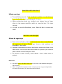
Figure 1 below shows a picture of the physical system (the “plant”) to control.
Figure 1. The physical system (plant) to control.
The control objective is to actuate on the motor such that the tip of the bar tracks a
specified angle.
P2  Describe reasons that cause this control objective to be nontrivial. (hints: Is it
possible to develop a table of electric tensions to apply to the DC motor such that the
bar tip moves to a constant position? What happens if a constant electric tension is
applied to the motor? Does feedback with a controller made of a single gain amplifying
the tracking error solve the problem? Think about the dynamics of the motor and the
bar. What is plausible rough distribution of the poles?).

Computer Control Laboratory Project
Page 5
Shaft
angular position 
Direction of
zero angular
position
Bar
deflection

Gear b ox
D/A
PA
M
A/D 0
A/D 1
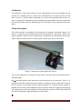
Figure 2. Schematic view of the hardware of the plant interconnected with the
computer control system. The motor M (including a gear box) is driven by the output
of a power amplifier PA and moves the flexible bar. The computer is interconnected
with the plant using AD and DA converters.
Figure 2 shows a schematic view of the interconnection of the plant (power amplifier
PA, DC motor with gearboxes M, and the flexible bar) with a computer.
The computer receives information about the angular position of the flexible bar tip
(given by the sum of the motor shaft angular position and the bar deflection) through
the AD converters. At each sampling time, al algorithm embedded in a computer
program reads this information and computes the value of the electric tension to apply
to the motor. This value is then applied through a D/A converter to the power
amplifier PA that drives the motor.
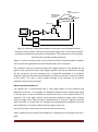
Measuring the bar deflection
The flexible bar is instrumented with a strain gage (figure 3) that measures the
deflection of the bar. A strain gage is a deflection variable resistor attached with glue
to the bar that is used to measure the mechanical forces on the material where it is
attached. The strain gage consists of an electrical resistance whose value changes
when its length varies. When the bar is deflected one of its faces is slightly stretched,
while the other is compressed, the changes being approximately proportional to the
bar tip deflection. For further details on strain gage sensors see
http://www.omega.com/literature/transactions/volume3/strain.html
Figure 3 below shows a detail of the flexible bar, indicating the mounting of the straingage.
Computer Control Laboratory Project
Page 6
Figure 3. Detail of the flexible bar showing the mounting of the strain-gage (indicated
by the red encirclement). The electronic circuit at the fixed part of the bar contains the
Wheastone bridge used to measure the electrical resistance of the strain gage.
D
Bar tip

Motor shaft
angular position

"Zero" direction
Figure 4. Schematic model of the flexible bar deflection.
With respect to the circular movement of the motor and the tip of the flexible bar,
consider the following quantities:




𝐿 [m], the bar length;
𝐷 [m], the length of the deflection of the bar tip;
𝛼[rad], the angular deviation of the bar tip with respect to the motor shaft
direction;
𝜃 [rad], the angle of the motor shaft direction with respect to a “zero”
direction.
Recall from basic Geometry that the value of an angle in radian [rad] is given by the
length of the corresponding arc of a circumference of radius of length to 1 in the
length unit used. Therefore, the relation of the angular deflection of the bar tip with its
deflection (measured along a straight line) is approximately given by
α=
Computer Control Laboratory Project
D
L
[rad].
Page 7
In practice, it is preferable to work in [degree] instead of [rad]. For that sake, observe
that the conversion between the same measure expressed in these units is made by
𝛼[𝑑𝑒𝑔𝑟𝑒𝑒] =
180
𝜋
𝛼[𝑟𝑎𝑑] .
Hereafter we will always use the angles expressed in degrees.
The issue of using the right units is fundamental. A space probe sent to Mars was
lost because part of the design team was using centimeters as unit length, while
the other part was using inches…
The total angle that defines the position of the tip of the flexible bar is
y= θ+α
[degree].
Flexible bar deflection transducer
The angle sensors provide a an electric tension that is an image of the corresponding
angle. In the case of the flexible bar, the sensor provides an electrical tension ∝𝑒 that
is related to the actual deflection angle 𝛼 by
𝛼 = 𝐾𝑏 𝛼𝑒 ,
where 𝐾𝑏 is a constant with units [degree/V].
Figure 5 shows a block diagram that relates the physical variable 𝛼 (angle) with its
electrical tension image ∝𝑒 .

1
e
Ke
Sensor
Figure 5. Relation between one angle and its measure given by the sensor.
In order to estimate the value of the constant 𝐾𝑏 , a sequence of experiments is done,
each experiment consisting of deflecting the bar by a known quantity and reading the
corresponding electrical tension.
In order to perform these experiments, the bar is rigidly attached to a support stand as
shown in figure 6. In the end of the stand there is a calibration “comb” with several
slots separated by 1⁄4 inch (1 inch = 2,54 cm) that, as shown in figure 7, allows to
deflected the bar by known quantities.
In the “ideal” situation, the electrical tension yielded by the sensor would be exactly
proportional to the deflection angle. In practice, this is not true because:
Computer Control Laboratory Project
Page 8


The relation is not exactly linear;
There are small random fluctuations from experiment to experiment.
Figure 6. The flexible bar mounted on its calibration rig.
Figure 7. The calibration “comb” for two different bar deflections: In rest, with no
deflection (left) and deflected to the left by one slot (right).
For these reasons one should:


Characterize the deviations with respect to the linear behaviors;
Make several experiments.
It is remarked that the linear behavior is only expected for relatively small
deflections. Large deflections may cause a permanent deformation of the bar and
should of course not be done.
Due to the deviations with respect to the ideal linear behavior, the value of the
constant 𝐾𝑏 corresponds to an average behavior. As such, this constant is estimated
from the set of data obtained in the different experiments using the least squares
algorithm.
The way to read the electrical quantities will be explained below in detail.
Shaft angle transducer
The shaft angle is measured with a rotation potentiometer whose axis is rigidly
connected with it. Figure 8 shows the internal scheme of the potentiometer being
used. A cursor (3) solidary with the potentiometer axis (4) (and therefore also with the
motor shaft) slides over a coiled resistive wired (1). When the cursor moves, the
resistance varies in a way that is proportional to the angle of the contact. An electric
Computer Control Laboratory Project
Page 9
circuit transforms this resistance in an electric tension value. Indeed, the resistive
element is powered at the extremes by a voltage of +5V (point 5) and -5V (point 9) and
therefore, depending on the cursor position, the output voltage has a value between 5V and +5V.
It is remarked that, since there are no mechanical stops at the extremes of the
resistance (end of course), the measured voltage repeats itself every whole rotation of
the cursor.
Figure 8. The internal scheme of the potentiometer used to measure the shat angle.
Therefore, the shaft angle 𝜃 is approximately given as a function of the sensor output
𝜃𝑒 by
𝜃 = 𝐾𝑝 𝜃𝑒 ,
where 𝐾𝑝 is a constant with units [degree/V].
It is remarked that, due the coiled structure of the resistance, there is a quantization
effect that causes the resistance to vary in a staircase form when the angle varies.
Before proceeding to the estimation of the transducer constants from plant data, the
use of the data acquisition and control software is explained.
Tachometer
The motor is also coupled with a tachometer that measures its angular velocity.
Similarly, the angular velocity of the motor 𝜔 [degree/s] is related to the tachometer
measure 𝜔𝑒 by
Computer Control Laboratory Project
Page 10
𝜔 = 𝐾𝑡 𝜔𝑒 ,
where 𝐾𝑡 is a constant with units [degree/s/V].
3.Software for data acquisition and control
To carry out data acquisition (reading data from the plant sensors connected to the
A/D converters) and process control (sending commands to the actuator, connected to
the D/A converter) the software "Matlab" + "Simulink" with toolboxes "Real-time
Workshop" + "Real-time Windows Target" will be used.
With "Simulink" it is possible to design data acquisition and control systems through a
simple graphical interface and with plenty of features. The "Real-time Workshop"
allows to transcript Simulink diagrams to C code and compile it to a target platform.
Finally, the "Real-time Windows Target" allows running real-time models in a
computer with the Windows operating system and synchronize the “time of the
computer” with the “real time” of the plant.
Although not essential to complete this work, the student is advised to consult the
manuals of these software tools, made available on the website of the course. In the
following lines, a brief description of the software to be used is presented.
Simulink
Simulink is a simulation environment that works in conjunction with Matlab and allows
simulations of dynamical systems in non-real time (simulated mode). There are several
component libraries (blocksets) that can be interconnected in easy and intuitive ways,
similar to a block diagram
In particular, there are components that allow to simulate dynamic systems, signal
generators, signal viewers and communicate with various I/O card, including the ones
to be used in this work.
However, since Simulink by itself does not allow to carry out simulations with a
synchronously real clock, it is necessary to rely on the Real-time Workshop "Tools" and
"Real-time Windows Target" kernel when using blocks that interface with A/D and D/A
converters. See the user manual of Simulink, available on the website of the discipline.
Real-Time Workshop
The Real-Time Workshop tool allows to transcript automatically Simulink models to C
code adapted to diverse hardware and software platforms. The code, when compiled,
generates an executable program that run the Simulink model in a separate process,
without graphical interface.
Computer Control Laboratory Project
Page 11
It is however possible to save and display the signals available in the model, as well as
to modify the properties of the blocks, using the Simulink external mode. In this mode,
the Simulink can communicate with the process executable to get/send data and
reconfigure the parameters of the simulation.
Real-Time Windows Target
With the Real-Time Windows Target tool, the C code generated by Real-Time
Workshop can be compiled for the Windows platform and run in real time.
For a good understanding of the process of creating code in real time, using all the
tools behind described, it is essential to consult the user manual of the Real-time
Windows Target, available on the website of the discipline. We recommend in
particular reading the chapter "Basic Procedures". Nevertheless, it is remarked that
reading these documents is not essential to perform this project.
 Tasks to be performed at the laboratory
Number of 3h laboratory sessions: 1
This introductory session is formatted as a tutorial. As such, few previous knowledge of
Matlab/SIMULINK will be required. All the necessary steps to configure the simulations
are quite detailed.
Since some of the procedures are repeated several times throughout the work, we
strongly advise the students to draw up a "check-list" based on the tasks performed,
synthesizing the procedures required to configure a real-time simulation, configure the
recording of data in the workspace, configure the elements viewers, etc. With these
working procedures, work efficiency will be greatly increased.
A – Generation, viewing and recording signals.
1. Open the SIMULINK. Open the MATLAB (version 7) and run the command
<<simulink>>. The window "Simulink Library Browser" will be opened.
2. Create a new model. In the menu "Simulink Library Browser", choose File-NewModel, or press CTRL + N. This opens a graphical window where you will enter
and connect the various operational blocks.
3. Insert and configure a block signal generator. In the selection tree to the left of
the window "Simulink Library Browser" choose "Simulink-Sources". Drag an
element "Signal Generator" for the model window. Open the element (double
click) and configure it to generate a square wave 2 volt amplitude and
frequency 2 Hz
4. Insert and configure a block signal Viewer. In the selection tree choose
"Simulink-Sinks" and drag an element "Scope" to the model window. Open the
item, and click the toolbar "Parameters" (second from left). In the tab
Computer Control Laboratory Project
Page 12
"General" configure "Tick Labels-All", "Sampling-Sample Time" and choose as
sampling period 1 millisecond (0.001). In the tab "History" remove "Limit date
selection points to last" and select "Save data to workspace". The data
presented in this element will be exported to the matlab workspace at the end
of the simulation. Choose the name of the variable "input" and data format
“Structure with time".
5. Configure and run the simulation. Connect the "Signal Generator" element to
the element "Scope". Start the simulation ("Simulation-Start" menu or CTRL-T).
Observe the result of the simulation in the viewer element "Scope"
6. Showing signals in workspace. Confirm that the workspace of matlab has the
"input" variable. Access the signal with the command "plot" and confirm that is
identical to that observed in the "Scope": >> plot (input., input.signals.values)
7. Save data from the workspace. Save the data file (see command "save") in
order to generate the graph "offline.
B – Sending commands to the motor.
8. Insert a block D/A to send commands to the motor. In the selection tree select
"Real-time Windows Target" and drag the "Analog Output" element to the
window of the template created.
9. Configure the block D/A. To see which data acquisition card is in use at the
laboratory bench, run the utility "Measurement & Automation" which you can
find on the Desktop. In the directory tree that appears on the left side of the
main window, choose "Devices and Interfaces"/"NI-DAQmx Devices", showing
the type of graphics card installed (e.g. NI PCI-6221 or PCI-MIO6040E). Make a
note of the type of card. Then go back to Simulink, open the D/A block and
select the appropriate board. Set the sampling period (sample time) to 1
millisecond (0.001). Set the output channel 1. Voltage ranges should be
configured between -10 and 10V and the data type as "voltage". The initial and
final values should be set to 0. Connect the signal generator to this block.
10. Configure the simulation to work in real-time In the menu "Simulation" select
"Configuration Parameters" or CTRL-e. This opens a dialog window. In the
Solver option-> Type choose “Fixed-step". In "Hardware Implementation->
Device Type" choose "32-bit real-time Windows Target". In "Real-time
Workshop-> RTW system target file" choose "rtwin.tlc".
11. Configure Simulink external mode. In the menu "Tools" choose "External Mode
Control Panel ...". This opens a dialog window. Select "Signal & Triggering". This
opens a new window. In "Duration" enter the number of total samples required
for the simulation, in this case 10 sec X 1000 samples/sec = 10000 samples. Go
back to the model window and, in the menu "Simulation", select "External".
Computer Control Laboratory Project
Page 13
12. Build the model. In the menu "Tools" choose "real-time Workshop-Build
Model" or CTRL-B. Wait for the build to complete and verify that there are no
errors
13. In order to run the template, in the “Simulation" menu choose "Connect to
target". Ask the staff of the laboratory to check the operation of the system
and start the operation by pressing the button. Use the button  to stop.
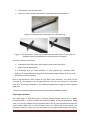
Figure 9 shows buttons in the SIMULINK project sheet that are useful to compile a
block diagram to be executed by real time workshop.
14. Observe the motor operation and register its behavior.
Figure 9. Buttons in the SIMULINK project sheet that are useful to compile a block diagram
to be executed by real time workshop. A: Connect To target; B: incremental Build; C.
Update Diagram
C – Reading signals from the sensors.
15. Insert A/D block to read the values of the sensors. In the selection tree select
"real-time Windows Target" and take two elements "Analog Input" to the
template.
16. Configuring the A/D block. Open the block and choose the acquisition card
installed in the machine. Set the sampling period (sample time) to 1 millisecond
(0.001). Set the input channel 1 (potentiometer) to one of the blocks and 3
(tachometer) to the other. Voltage ranges should be configured between -10
and 10V and the data type as "voltage".
17. Insert two blocks "Scope" to show the signals of the sensors. Configure them as
in point 4. Give them the names "tensao_pot" and "tensao_taq" respectively..
18. Recompile the model..
19. Run the model. Confirm with the teacher wether all is well before beginning
the simulation. Observe and register the graphics of the time evolution of the
potentiometer voltage and of the tachometer.
20. Record data. Make sure that the vector variables "tensao_pot" and
"tensao_taq" are available in the workspace of Matlab and save them to a file.
D – Sensor Calibration.
Computer Control Laboratory Project
Page 14
21. Apply a step signal (1 volt) to the motor. Acquire and record the voltages
obtained by the potentiometer and the tachometer. From the data obtained,
calculate the calibration factor 𝐾𝑝 [degree/volt] and 𝐾𝑡 [degree/s/volt], that
make it possible to convert sensor measurements in volt for degrees and
degree/sec, respectively.
22. Similarly, make a set of experiments to estimate the calibration factor 𝐾𝑏
[degree/volt] for the bar deflection. Use the procedure described in relation to
figures 6 and 7.
P3  Write a report about your activities, including:


Comment on the motor operation. Explain in particular why their angular
position never stabilizes when its command signal is constant.
Explain the procedure carried out to perform sensor calibration. Include in the
report:
o The Simulink block diagram used;
o Plots of the sensor and command signals;
o The auxiliary calculations and/or the graphics used to compute the
conversion factors 𝐾𝑝 [degree/volt], 𝐾𝑡 [degree/s/volt], and 𝐾𝑏
[degree/volt].
o Plot on the same graphic the experimental points obtained for the bar
deflection and the linear relation assumed to hold between the bar
deflection and the sensor electric tension for the value of 𝐾𝑏 that you
have estimated.
Important: When writing your reports, do not forget to display the units in both
axes of graphs and to write appropriate captions to identify all the graphs and
diagrams, explaining the experimental conditions to which they refer.

4. Plant model identification.
Plant model identification aims at producing a model to be used for control design. For
that sake, the following steps are performed:
1. Select an input signal (for instance a square wave or a PRBS) and perform an
experiment in which the plant is excited with it. Register the data. For this sake,
use the data acquisition facilities of SIMULINK that you have learned how to
use in section 3, and write an appropriate SIMULINK block diagram. Use a
sampling interval of 0,02 s (sampling frequency of 50 Hz). Observe that the
motor+gear box has a dead zone.
2. The plant output (angular position of the flexible bar tip) data has to be treated
in order for the identification algorithm to work properly
Computer Control Laboratory Project
Page 15
a. Differentiate the plant output to remove the integrator associated to
the motor.
b. Remove constant offsets in data using the MATLAB function detrend
c. Filter the output to eliminate high frequency dynamics and noise that
fall outside the frequency band in which the model is to be valid. For
that sake use the commands
Ts=0.02; % sampling interval [s]
alpha = 0.8;
% filter pole
Afilt = [1, -alpha];
Bfilt = [1-alpha, -1+alpha]/Ts;
Filtered_outproc = filter(Bfilt,Afilt,nonfilt_outproc);
3.
4.
5.
6.
Identify an ARMAX model using the function armax;
Add the integrator to the model (use the function conv)
Convert the model to state-space form using the function tf2ss
Validate the model in various forms.
a. Compare data that has not been used for identification with the result
obtained by simulating with the model using as input the same input
used to excite the system;
b. Look at the simulated time response and discuss its plausibility;
c. Look at the frequency response and discuss its plausibility.
7. Review the process, changing the values of some parameters (filter pole,
assumed model orders, sampling interval).
The final result is a discrete time state space model that relates the input to the motor
with the flexible bar tip position, that is of the form
x(k + 1) = Ax(k) + Bu(k)
(3-1)
𝑦(𝑘) = 𝐶𝑥(𝑘) + 𝐷𝑢(𝑘)
(3-2)
where 𝑢 (scalar) is the motor excitation, 𝑦 (scalar) is the flexible bar tip angular
position, 𝑥 (𝑛 × 1) is a column vector and 𝐴 (𝑛 × 𝑛), 𝐵 (𝑛 × 1), 𝐶 (1 × 𝑛) and 𝐷 = 0
(scalar) are matrices of compatible dimensions, 𝑛 being the dimension of 𝑥. These
matrices form the input to the next phase of the project, concerned with controller
design. The index 𝑘 denotes discrete time.
 Experiments to perform at the laboratory
Number of 3h laboratory sessions: 2
Execute the procedure listed above to obtain a model. Write MATLAB scripts to
automate the procedure. Explore several options in a critical way. Take into
consideration the issues you have to answer in the report.
P4  Write a report about plant model, including:

Explanation on the tests performed on the plant to obtain the data used for
identification. Discuss the results obtained with different types of excitation
Computer Control Laboratory Project
Page 16








signals and the effect of very small amplitude and very large amplitude
excitation signals;
Discussion of the sampling frequency;
Effect on identification of filtering the data;
Explanation on how the pole at the origin has been dwelt with;
Discussion on how the model orders have been decided. Take into
consideration that the plant results from the interconnection of a DC motor
and the flexible bar and discuss the models needed for each of them;
Description of the final ARMAX model;
Description of the final state-space model.
Characterization of the plant open loop pole-zero plot, frequency response and
time response of the model.
Model validation;

5. Controller design.
In this section, the state-space model identified on section 4 is used to design a LQG
controller.
The controller consists of a state feedback control law whose gains are selected such
as to minimize a quadratic cost. The controller gains are designed on the basis of the
state model (3-1), (3-2) that has been identified. This is the LQ control law.
Since the state of the plant is not available for direct measurement, it is estimated with
a Kalman filter. The kalman filter receives as input the plant input and output and
yields as it output an estimate of the plant state.
The equations of the algorithm that are required to perform this work are described
hereafter. Further details can be seen in the book
G. F. Franklin, J. D. Powell and M. Workman. Digital Control of Dynamic Systems. 3rd
ed., Addison Wesley, 1998, chapter 9 “Multivariable and Optimal Control”.
LQ control law.
The control law that generates the manipulated variable 𝑢 for the state model (3-1),
(3-2) such as to minimize the steady-state (or infinite horizon) quadratic cost
𝑇
𝑇
𝐽 = ∑∞
𝑘=1 𝑥 (𝑘)𝑄𝑥(𝑘) + 𝑢 (𝑘)𝑅𝑢(𝑘),
(5-1)
where 𝑄 ≽ 0 (means 𝑄 is positive semi-definite)and 𝑅 ≻ 0 (means 𝑅 is positive
denite) is given by the state feedback
𝑢(𝑘) = −𝐾𝑥(𝑘),
Computer Control Laboratory Project
(5-2)
Page 17
where the vector of feedback gains 𝐾 (1 × 𝑛) is computed by
𝐾 = (𝐵 𝑇 𝑆𝐵 + 𝑅)−1 𝐵𝑇 𝑆𝐴.
(5-3)
The matrix 𝑆 (𝑛 × 𝑛) is the positive definite solution of the algebraic Riccati equation
(ARE)
𝐴𝑇 𝑆𝐴 − 𝐴𝑇 𝑆𝐵(𝐵 𝑇 𝑆𝐵 + 𝑅)−1 𝐵𝑇 𝑆𝐴 + 𝑄 = 0.
(5-4)
If there exists a 𝐾 such that the closed-loop system that results from coupling (3-1)
with (5-2), then it can be found by (5-3), (5-4).
For the purposes of this work, The LQ gain is computed using the MATLAB function
dlqr. Use the MATLAB help to know how to use this function.
The function also computes the closed-loop eigenvalues, given by the eigenvalues of
𝐴 − 𝐵𝐾. This result is an important piece of information.
The main “tuning knob” for the designer when using LQ control are the matrices 𝑄 and
𝑅. For a SISO plant, if the output 𝑦 is to be regulated, then
𝑄 = 𝐶 𝑇 𝐶.
(5-5)
The weight 𝑅 reduces to a scalar. Changing 𝑅 adjusts the type of response yielded.
Indeed, the poles of the closed-loop system are the stable roots of the root square
locus. In general, decreasing 𝑅increases the bandwidth of the control system. Thus,
decreasing 𝑅 has the advantage of making the response of the close loop faster, but
the disadvantage of exciting plant modes that are not modeled.
Warning: Do not confuse dlqr, that solves the LQ problem in discrete time (the
formulation used here) with the function lqr that solves a similar problem in
continuous time (not considered in this work).
Kalman filter.
The Kalman filter aims at estimating the plant state from the observation of the plant
input and output. It assumes that the plant model is modified by the inclusion of
“disturbance” or “noise” inputs, becoming
x(k + 1) = Ax(k) + Bu(k) + 𝑤(𝑘) ,
(5-6)
𝑦(𝑘) = 𝐶𝑥(𝑘) + 𝐷𝑢(𝑘) + 𝑣(𝑘).
(5-7)
The signal 𝑤 is the process noise and the signal 𝑣 is the sensor noise.
The equations of the Kalman filter are given by
𝑥̂(𝑘|𝑘 − 1) = 𝐴𝑥̂(𝑘 − 1|𝑘 − 1) + 𝐵𝑢(𝑘 − 1)
Computer Control Laboratory Project
(5-8)
Page 18
𝑥̂(𝑘|𝑘) = 𝑥̂(𝑘|𝑘 − 1) + 𝑀(𝑦(𝑘) − 𝐶𝑥̂(𝑘|𝑘 − 1)).
(5-9)
These equations are interpreted as follows:


Equation (5-8) computes what you expect the state to be at time 𝑘 given the
previous estimate 𝑥̂(𝑘 − 1|𝑘 − 1), the input sample applied, 𝑢(𝑘 − 1), and the
knowledge about the state dynamics.
Then, this prediction is corrected by a term that is proportional to what you
expect the output to be given the state prediction, 𝐶𝑥̂(𝑘|𝑘 − 1), and what is
actually observed for the value of 𝑦(𝑘).
The proportionality constant vector 𝑀 is called the Kalman gain. It is computed so as to
optimize a quadratic cost. In this work, the Kalman gain is computed using the MATLAB
function dlqe. Use the MATLAB help to know how to use this function. Again, do not
make a confusion with the function lqe that computes the Kalman filter gain for the
continuous time case.
Instead of using (5-8) and (5-9) it is possible to eliminate the prediction from (5-8) and
(5-9) and propagate the estimate using
𝑦(𝑘)
𝑥(𝑘|𝑘) = Φ𝐸 𝑥(𝑘 − 1|𝑘 − 1) + Γ𝐸 [ − − − ],
𝑢(𝑘 − 1)
(5-10)
Φ𝐸 = 𝐴 − 𝑀𝐶𝐴
(5-11)
where
and
Γ𝐸 = [𝑀
| 𝐵 − 𝑀𝐶𝐵].
(5-12)
Loop transfer recovery (LTR).
The computation of the Kalman gain requires the covariance matrices of the noises
entering the model. These are 𝑄𝑤 = ℰ(𝑤𝑤 𝑇 ) and 𝑅𝑣 = ℰ(𝑣𝑣 𝑇 ). In this case, 𝑅𝑣 is a
scalar. Instead of trying to estimate these noise covariances from plant data, we are
going to use them as “tuning knobs”. Thus, we make the choices
𝑄𝑤 = 100𝐼
and
𝑅𝑣 = 1.
LQG controller structure
The LQG controller is obtained by coupling a LQ controller with a Kalman filter and
replacing the state by its estimate. This controller has the structure shown in figure 10.
Computer Control Laboratory Project
Page 19
u(k)
r(k)
Plant
N
y(k)
z-1
u(k-1)
Kalman
filter
K
Figure 10. Structure of the LQG controller.
The constant 𝑁 is such that, in closed-loop, the gain from the reference 𝑟 to the
output 𝑦 is equal to 1. For a state of dimension 5 it can be computed by the MATLAB
code:
N = inv([A-eye(5,5), B; C,0])*[zeros(5,1);1];
Nx = N(1:5,:);
Nu = N(6,:);
Nbar = Nu+K*Nx;
See the reference book on page 313.
 Experiments to perform at the laboratory
Number of 3h laboratory sessions: 2
Design a LQG-LTR controller according to the procedure explained and test it. Start by
testing the controller designed in simulation using the state-space model that has been
identified in section 4. Explore several options by changing the weight matrix 𝑅. Start
by making 𝑅 = 100.
When you think you have a satisfactory result, try it on the real system. (Think about
what are the features of the time response you look at to consider them
“satisfactory”). What happens when you increase 𝑅𝑣 ?
Write MATLAB scripts and SIMULINK block diagrams to automate your design.
P5  Write a report about controller design and testing of the controlled system,
including:






The MATLAB scripts that must include comments;
The block diagram used to control the system;
Comment on the choice of the weights on the quadratic cost when using the
LQG design approach. Include the root-square locus;
Effect of the choice of the noise covariance matrices in a LTR framework;
Resulting closed-loop frequency response and time response;
Effect of the inclusion of a pre-filter;
Computer Control Laboratory Project
Page 20

Discuss how do you evaluate the performance of your control system and what
are the limits of performance.

–
Computer Control Laboratory Project
End of the project –
Page 21