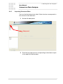
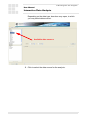
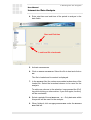
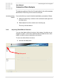
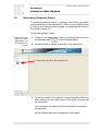
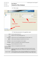
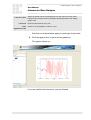
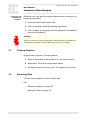
1
Interactive Data Analysis User Manual Version V1.1 MEDAV GmbH 2008 MEDAV GmbH Gräfenberger Straße 34 D-91080 Uttenreuth Tel.: +49-(0)9131/583-0 Document Interactive Data Analysis - User Manual Version V1.1, Issue 10/29/2008. Copyright This document is protected by copyright laws. Trademarks For better legibility, in this document marking of trademarks is waived. This should not mislead to the assumption that these trademarks are to be used freely by anybody. Contact for Errors or Complaints The product is the result of highest possible effort for reliable function and easy usability. When editing this document, greatest importance was attached to completeness and correctness. Even so, if you find an error or incompleteness, please contact MEDAV GmbH, Tel.: +49 9131/583-0, eMail: [email protected]. The document is subject to change without prior announcement. User Manual Interactive Data Analysis Table of Contents 1 2 3 About this Document 5 1.1 Purpose of this Document 5 1.2 Using this Document 5 1.3 Special Representations 5 Introduction 7 2.1 Overview 7 2.2 System Requirements 8 Working with the Program 9 3.1 Requirements of the Data Material 9 3.2 Starting the Program 9 3.3 Overview of the Process 3.3.1. Structure of the Program 10 3.3.2. Using Online Help 12 3.4 Loading and Selecting Data 4 10 12 3.4.1. Selecting Period of Time of Data 13 3.4.2. Using Data from the Data Base 13 3.4.3. Importing Structured Data 19 3.4.4. Importing Data Without Structure 22 3.5 Applying the Analysis Procedure 27 3.6 Generating Graphical Output 31 3.7 Printing Graphics 34 3.8 Exporting Data 34 3.8.1. Exporting Graphics 35 3.8.2. Exporting Tables 35 Methods 37 4.1 Basic Statistics 37 4.2 Fast Fourier Transformation and Short Term FFT 38 4.3 Polynomial Interpolation 38 4.4 Sinus Approximation 39 4.5 Spline Interpolation 40 Version V1.1 3 User Manual Interactive Data Analysis 4 4.6 Up-/Downsampling and Time Shift 41 4.7 Power Spectrum 41 4.8 Correlation/Autocorrelation 42 4.9 Comparison 43 4.10 Time-Frequency Analysis by Wavelets 44 4.11 Filters 44 Index 47 Version V1.1 User Manual 1 About this Document Interactive Data Analysis 1 About this Document This chapter provides an overview of this document and information on its use. 1.1 Purpose of this Document This manual contains information about the structure, function and operation of the program. It is intended to enable and to facilitate your work and the usage of the program. Read and use the manual if you work with the program and operate the software. 1.2 Using this Document This manual consists of: • an overview of program • an overview of the process of analyzing signals with the system • detailed operating instructions how to use the system This manual does not contain information about the data or data formats, and not about procedures applied for analysis. This type of knowledge is assumed to be present to the users of program and must be achieved from other sources. 1.3 Special Representations Cross references Controls Cross references are displayed as shown here. The steps in the chapters containing step wise instructions partially refer to on-screen controls. These are, e. g.: • Version V1.1 buttons to be clicked with the mouse 5 User Manual 1 About this Document Interactive Data Analysis • lists from which elements are to be selected (drop down list fields etc.) • fields into which text is to be entered (text fields) All these carry labels which are represented as shown here. Keys If keys or combinations of keys are required for operation, then this is represented as follows: • [Ctrl + a] means that the "Ctrl" key and the "a" key (lower case) must be pushed simultaneously • [Return] means that the "Return" key must be pushed. • [Shift] means that the "Shift" key must be pushed The steps of the instructions are numbered and should be carried out in the given order if nothing else is denoted. 6 Version V1.1 User Manual 2 Introduction Interactive Data Analysis 2 Introduction The program allows for interactive analysis of geodetic time series data. 2.1 Overview Users can apply standard methods of time series analysis on geodetic data sets. The data sets can be selected by means of a graphical user interface and be loaded into an analysis application. Predefined data sets of different origin are available as well as the functionality to use own data sets. The procedures intended to be applied on the data sets can be selected and be parameterized. Result data can be presented as numeric data or visualized graphically, whereby users can widely control the graphical output. The software is divided into three operational sections separated by tabs. The sections are: • Data – select data file and a period of time of which data sets are to be analyzed • Procedure – select a procedure (method) to used for analysis and set its parameters • Output – set the output parameters and view the numerical and/or graphic results Another section About presents information about the program operator, disclaimer and imprint. The following chapters show how to operate the program. The different procedures and their outputs are described in separate documents. Version V1.1 7 User Manual 2 Introduction Interactive Data Analysis 2.2 System Requirements The program can be run platform independently in a browser. Sufficient computing power is required on the client computer or on the server. The program needs Java Runtime environment Version 1.5 on the client computer. 8 Version V1.1 User Manual 3 Working with the Program Interactive Data Analysis 3 Working with the Program Follow the instructions of this chapter to operate the program. 3.1 Requirements of the Data Material Data of different origin and use are available by the software, however, you can also use own data. The program can use data in CSV and XML table formats. The first column of the table is always used as parameter for the xaxis. 3.2 Starting the Program The program is run in a web browser. Note(s): Response time of the program strongly depends on the quality of the internet connection. To start the program: 1. Start a web browser and enter the URL (internet address) of the program as you received by your software operator. Version V1.1 9 User Manual 3 Working with the Program Interactive Data Analysis 3.3 Overview of the Process This section briefly explains how to turn numerical geodetic time series data into expressive overview graphics. 3.3.1. Structure of the Program The program is subdivided into panels, which can be invoked by the tabs at the upper edge of the program window. They are intended to be used one after the other from the left to the right, therefore, alternatively they can also be invoked by forward/ backward buttons switching between subsequent panels. Tabs to switch between panels Forward/Backward Buttons 10 Version V1.1 User Manual 3 Working with the Program Interactive Data Analysis The functions provided by the tabs are available only if the previous steps are completed successfully. The panels provide the following functions: • Data – select data file and a period of time of which data sets are to be analysed • Procedure – select a procedure (method) to be used for analysis and set its parameters (loaded data required) • Output – set the output parameters and view the numerical and/or graphic results (results from completed procedure required) Another panel About contains information about the program and the operator of the service. It is not needed to operate the program, however, it may contain information of your interest. The panels provide white areas in the left, with which you control the program as follows: • In the upper white field select between the different items offered depending on the current program status. For example: when the Procedure panel is active, select the procedure to be used. • In the lower white field see, select, and delete data objects loaded for analysis, depending on the program status (workbench). For example, when the Procedure panel is active, select data for graphical output. In the larger right area of the program window, enter data or view outputs, depending on the situation. Follow the detailed steps described in the sections below: • Loading and Selecting Data on page 12 • Applying the Analysis Procedure on page 27 • Generating Graphical Output on page 31 Note that online help is available for the program, as described in the next subsection. Version V1.1 11 User Manual 3 Working with the Program Interactive Data Analysis 3.3.2. Using Online Help The program provides online help in different situations: • Each panel features a Help button. Click on it to call for help about the currently active panel. • In the Procedure panel you may push the [F1] button to call for help about the specific procedure. Help is displayed in a standard web browser or in a specific help viewer, depending on the type of installation. 3.4 Loading and Selecting Data You can decide to use predefined data from the data base, or own structured data or own data without structure. Note(s): The meaning of predefined input data is subject of other documentation. In doubt, ask the operator of the software. This document deals with the program operation only, on which data have no effect. See 12 • Using Data from the Data Base on page 13 • Importing Structured Data on page 19 • Importing Data Without Structure on page 22 Version V1.1 User Manual 3 Working with the Program Interactive Data Analysis 3.4.1. Selecting Period of Time of Data You will note that you can select a period of time of the data at each stage of the program. The reason is that different time data can be required in the different stages, but need to be loaded only once. Once loaded, the period of time can then be reduced according to your needs. Example: Assume you want to analyse • EOP/Pole/x from 1970 to 1980 • EOP/Pole/y from 1975 to 1985 In this case, you first load the complete EOP/Pole data over the complete period of time from 1970 to 1985. Then you apply analyse procedures on them or restrict the period of time, depending on the type of data or procedure. When plotting the data, you may restrict the time period again for the graphics displaying results according your requirements. 3.4.2. Using Data from the Data Base In the Data panel you select the data to be analysed. They are arranged in tables presented in form of a so-called “tree”, that is: the data are grouped in different levels: Version V1.1 • product groups (Basic procedures, Correlation, Approximation etc.) • products, which can be in turn subdivided into groups (depending on the selected product group: Basic statistics, Autocorrelation, etc.) • data vectors (name of a table column, depending on the selected product) 13 User Manual 3 Working with the Program Interactive Data Analysis To load predefined data from the data base, proceed as follows: 1. Activate the Data panel. Data panel 14 Version V1.1 User Manual 3 Working with the Program Interactive Data Analysis 2. Click on an input data source in the upper left field Products. Depending on the data type, branches may open, in which you may select data sources: Available data sources 3. Click to select the data source or sources for the analysis. To add more columns to the selection: keep pressed the [Ctrl] key while clicking on other entries. If you click again, the entry will be unselected. To add a complete group, just click this group. All elements of the group will be selected. Version V1.1 15 3 Working with the Program User Manual Interactive Data Analysis 4. Enter start time and end time of the period to analyse in the date fields. Start and End time Load button Progress bar 5. Click the Load button to load them into the program. A progress bar indicates the loading status and shows when the load process is complete. The data are listed in a table for selection. 6. Select the data to analyse in the Product field. They refer to the columns of the table. To add more columns to the selection: keep pressed the [Ctrl] key while clicking on other entries. If you click again, the entry will be unselected. 7. Again you have the chance to restrict the data to be analysed by entering a start and end time. 16 Version V1.1 3 Working with the Program User Manual Interactive Data Analysis 8. Click on Apply selected data. Start and End time Select Data Apply selected data button Version V1.1 17 User Manual 3 Working with the Program Interactive Data Analysis The data are displayed in the lower white field (workbench) when loading is finished: Loaded data in the workbench 9. You can repeat the steps until all required data are in the workbench. When all the correct data are in the workbench, you proceed with setting up the analysis procedure. see Applying the Analysis Procedure on page 27. Correcting wrong entries If you notice that you want to delete loaded data, proceed as follows: 1. Select the data entry to delete in the workbench and right click the data entry. 2. Select Delete from the context menu showing up. The entry will be deleted. 18 Version V1.1 User Manual 3 Working with the Program Interactive Data Analysis 3.4.3. Importing Structured Data You can load structured own data if their structure corresponds to the sources in the data base. 1. Activate the Data panel. Data panel 2. Click the input data source corresponding to the data to import in the upper left field Products. Version V1.1 19 User Manual 3 Working with the Program Interactive Data Analysis Depending on the data type, branches may open, in which you may select data sources: Available data sources 3. Click to select the data source for the analysis. 20 Version V1.1 3 Working with the Program User Manual Interactive Data Analysis 4. Enter start time and end time of the period to analyse in the date fields. Start and End time Load local file checkmark 5. Activate Load local file. 6. Click on Choose and load file. Select the file to load and click on OK. The file is loaded and its content is displayed. 7. In the Products field, the columns are added as branches of the loaded file. Select the branches/columns to be used for the analysis. To add more columns to the selection: keep pressed the [Ctrl] key while clicking on other entries. If you click again, the entry will be unselected. 8. Select a period of time at Date from ... to .... Only data sets within this period will be used for the analysis. 9. When finished, click on Apply selected data under the Selected Data field left. Version V1.1 21 User Manual 3 Working with the Program Interactive Data Analysis The data are gathered from the file and added to the white Selected data field left. Now they can be used for analysis. Correcting wrong entries If you notice that you want to delete loaded data, proceed as follows: 1. Select the data entry to delete in the workbench and right click the data entry. 2. Select Delete from the context menu showing up. The entry will be deleted. 3.4.4. Importing Data Without Structure You can load data without structure, that means: the data are arranged in a table. In this case, load the data and add structure information as table column separators and names. To use own data without structure: 1. Activate the Data panel. Data panel 22 Version V1.1 User Manual 3 Working with the Program Interactive Data Analysis 2. In the Products field, select Local Data | Generic CSV. The CSV Import panel shows up in the right, allowing for selection of a data file and specifying parameters. 3. Click on Choose and load file. Select the file to load and click on OK. The first line of the data table is shown in the text field. This maybe the line with the table header information (names of the columns) or it also maybe the first data line. Version V1.1 23 User Manual 3 Working with the Program Interactive Data Analysis Table structure configuration You can either use a predefined configuration or enter a configuration. The configuration specifies the column separator and the names of the columns. You can skip these steps if the first line of the table contains the column names anyway. To use a predefined configuration, load it from file: 1. Click on Load config. 2. Find the desired file and click on OK. The file is loaded. 3. Click on Apply. The configuration is applied to the loaded data. Alternatively specify the configuration: 1. Adjust the proper column separator and click the Next button. 2. Click in the first table cell under the table header and enter a name for the column. Repeat this for each column. 3. If you want to re-use the configuration later, save it to file. To do so, click on Save config, find a directory, enter a file name, and click on Save. 24 Version V1.1 User Manual 3 Working with the Program Interactive Data Analysis Converting and loading the file When configuration is finished, continue with converting the and loading the file: 1. Click on Convert. A progress bar indicates the loading status and shows when the load process is complete. 2. In the Products field, the columns are added as branches of the loaded file. Select the branches/columns to be used for the analysis. To add more columns to the selection: keep pressed the [Ctrl] key while clicking on other entries. If you click again, the entry will be unselected. Version V1.1 25 3 Working with the Program User Manual Interactive Data Analysis 3. Select a period of time at Date from ... to .... Only data sets within this period will be used for the analysis. Select Period of Time Select Data Apply selected data button 4. When finished, click on Apply selected data under the Selected Data field left. The data are gathered from the file and added to the white Selected data field left. Now they can be used for analysis. Correcting wrong entries If you notice that you want to delete loaded data, proceed as follows: 1. Select the data entry to delete in the workbench and right click the data entry. 2. Select Delete from the context menu showing up. The entry will be deleted. 26 Version V1.1 3 Working with the Program User Manual Interactive Data Analysis 3.5 Applying the Analysis Procedure You can set up and apply the analysis procedure only if you have loaded data into the workbench. If you did not yet, return to Loading and Selecting Data on page 12. Similar to the products in the data panel, the procedures are arranged in groups. Only those procedures can be selected which correspond to the loaded data type and for which a sufficient amount of data is loaded to the workbench. To set up and apply the analysis procedure: 1. Change to the Procedure panel, either by clicking its tab or click on the forward button in the Data panel. The Procedure panel becomes active. The available analysis methods are listed in the left upper white field. The other white field below still shows the data in the workbench: List of available procedures Loaded data in the workbench Version V1.1 27 3 Working with the Program User Manual Interactive Data Analysis Note(s): The meaning, effect, parameters, and the output of the procedures are subject of the descriptions shipped with these procedures. This document deals with the program operation only, on which the procedures do not have effect. 2. Select the data in the workbench, on which you intent to apply the procedure. 3. Select the procedure or procedure group in the upper left field Products by a click. Depending on the procedure, branches with procedures may open, of which you may select. If so, select the appropriate type of procedure. If not, return to selecting appropriate data. Only procedures are selectable which are suitable to the loaded data in the workbench. If you have selected the procedure prior to the data, inappropriate data become not selectable anymore (are greyed out) in the workbench. 4. The procedures may provide input parameters. Enter proper values for the intended analysis: Selected procedure Parameter(s) Selected data in the workbench Run button 28 Progress bar Version V1.1 User Manual 3 Working with the Program Interactive Data Analysis 5. When finished, click the Run button. Analysis starts. A progress bar indicates the status and shows when the process is complete. Afterwards distinct numerical result values are output, or tables of result values are listed and in the workbench: Numerical Results 6. Examine the numerical output whether it meets your expectations. If it is required to improve the results, return to altering the parameters or to load other data. This is described in the sections previous to this one. Version V1.1 29 User Manual 3 Working with the Program Interactive Data Analysis The procedure output data are available in the workbench: Procedure output in the workbench You can repeat the previous steps, to collect various data in the workbench. If the results are complete meet the expectations, continue with turning it into graphical output, as described in Generating Graphical Output on page 31. Otherwise repeat the previous steps. Correcting wrong entries If you notice that you want to delete data from the workbench, proceed as follows: 1. Select the data entry to delete in the workbench and right click the data entry. 2. Select Delete from the context menu showing up. The entry will be deleted. 30 Version V1.1 User Manual 3 Working with the Program Interactive Data Analysis 3.6 Generating Graphical Output To generate graphical output (= plotting), data and/or procedure output needs to be in the workbench. If this is not yet fulfilled, return to Loading and Selecting Data on page 12 or Applying the Analysis Procedure on page 27. To generate graphic output: Note that the upper white control field disappeared, only the workbench remained. 1. Change to the Output panel, either by clicking its tab or click on the forward button in the Procedure panel. 2. Select the data to display graphically in the workbench: Selected output in the workbench 3. To add more data to the selection: keep pressed the [Ctrl] key while clicking on other data entries. Click again, the entry will be unselected. You can repeat the steps until all required data to be plotted are selected. All the selected data will be displayed in the graphic. Version V1.1 31 3 Working with the Program User Manual Interactive Data Analysis 4. Click on Plot. Parameters for graphical output Apply button Plot button 5. Enter the parameters for the graphical output: Value Shows the data selected item. Color Adjust the color of the plotted graphic line. Line Style Marker Adjust the line style of the plotted graphic line (solid, dotted, etc.) Defines symbols displayed at data points on the curve. Title Text Enter a text that is displayed over the graphic. Plot grid Switch on or off whether a grid is desired in the graphic. X axis text Enter the label texts for the x-axis. X axis logarithmic scale Switch on or off logarithmic scale for x-axis. x axis max value Select the period of time to be displayed, here the lower start value. Data loaded and processed remain unchanged, this setting refers to the display graphic only. x axis as ’date’ 32 Enable to display the x axis in date format (MM/DD/YYYY). If disabled, the x axis is displayed in MJD format (Modified Julian Date, double integer value). Version V1.1 User Manual 3 Working with the Program Interactive Data Analysis x axis min value Y axis text Y axis logarithmic scale Select the period of time to be displayed, here the upper end value. Data loaded and processed remain unchanged, this setting refers to the display graphic only. Enter the label texts for the y-axis. Switch on or off logarithmic scale for y-axis. Note that not all parameters apply for each type of input data. 6. Click the Apply button to generate the graphic(s). The graphic shows up: If you are satisfied with the result, you are finished. Version V1.1 33 User Manual 3 Working with the Program Interactive Data Analysis Improving and Adding new Graphics Otherwise you may alter the output parameters by returning to entering the parameters: 1. If desired, select other output data. 2. Click on Plot and change the desired parameters. 3. Click on Apply. A new graphic will be generated and added to the previous graphics. Note(s): Note you can return to any previous panel to alter selections in the data/procedure/output control field or in the workbench to improve your results. 3.7 Printing Graphics Graphics can be printed. To print graphics: 1. Right click the data in the workbench in the Output branch. 2. Select Print. The printer control panel opens. 3. Set up the printer and click on OK. The graphics are printed. 3.8 Exporting Data You can export graphics as well as table data. See 34 • Exporting Graphics on page 35 • Exporting Tables on page 35 Version V1.1 User Manual 3 Working with the Program Interactive Data Analysis 3.8.1. Exporting Graphics Graphics can be exported as PNG or JPEG file. To export graphics data: 1. Right click the data in the workbench in the Output branch. 2. Select Export JPG or Export PNG. 3. Find a directory and enter a name for the file. 4. Click on Save. 3.8.2. Exporting Tables Tables can be exported as tables in CSV format. To export table data: 1. Right click the data in the workbench in the Procedure branch. 2. Select Export CSV. 3. Find a directory and enter a name for the file. 4. Click on Save. Version V1.1 35 User Manual 3 Working with the Program Interactive Data Analysis 36 Version V1.1 User Manual 4 Methods Interactive Data Analysis 4 Methods In this chapter, the methods are listed and described. 4.1 Basic Statistics This method extracts statistical features from the input signal. It evaluates a time series and extract statistical features to display them textually. This method provides no input parameters. Output parameters are: Maximum Mean Median Contains the maximum value of the curve. Contains the mean (arithmetic average) value of the curve. Contains the median value of the curve. Minimum Contains the minimum value of the curve. Standard Deviation Contains the standard deviation value of the curve. Timepoint Maximum Contains the time stamp of the maximum value of the curve. Timepoint Minimum Contains the time stamp of the minimum value of the curve. Input minus max Contains the time series computed from the input time series minus the maximum value. Input minus mean Contains the time series computed from the input time series minus the mean (arithmetic average) value. Input minus median Contains the time series computed from the input time series minus the median value. Input minus min Version V1.1 Contains the time series computed from the input time series minus the minimum value. 37 User Manual 4 Methods Interactive Data Analysis 4.2 Fast Fourier Transformation and Short Term FFT This method applies an FFT on the time series input. Input parameters are: FFT Length Select an FFT length from 2 to 65536 in steps of powers of two. The signal is filled up with zeroes up to the specified length. Window Type Select a Window type: • None • Square • Hamming • Hanning Output parameters are: Amplitude Contains the amplitude series values (FFT magnitude). Frequency Contains the frequency series values. Imaginary Part Phase Real Part 4.3 Contains the imaginary part series values. Contains the phase series values (FFT phase, prograde and retrograde). Contains the real part series values. Polynomial Interpolation This method uses a Levenberg-Marquardt algorithm to approximate the input time series to a polynome. The degree of the polynome can specified. The polynome is estimated in the sense of the least square of the data. The output time series are displayed at the same sampling times as in the input signal time series. The prediction deviation (residual) is the difference between predicted polynome and the input time series. The method checks whether the polynome degree is in line with the number of the available values of the time series and issues an error message otherwise. 38 Version V1.1 4 Methods User Manual Interactive Data Analysis The estimation of the polynome coefficients of higher degree is numerically instable, therefore, the coefficients are not estimated directly but the Chebychev coefficients are computed instead. The polynome estimation is stable, when the time axis is transformed so that the polynome arguments between -1 and +1 are used. The coefficients of the resulting polynomes estimated by least squares are returned. Additionally, the time axis transformation is reversed and the classical polynome coefficients of the polynome form are returned: a0 + a1t + a2t2 +... Inputs of the method are: Degree Specify a degree of the polynome. Outputs of the method are: Chebychev Coefficients Contains the Chebychev coefficients of the polynome. Coefficients Contains the coefficients of the polynome. Residual 4.4 Contains the residual. X Contains the original time values. Y Contains the result values of the polynome interpolation. Sinus Approximation This method conducts a sinus approximation. A frequency is specified by a parameter. The method estimates phase and amplitudes. The estimation is conducted using the least squares method. The target function is: y = A × sin ( 2πfx + φ ) The frequency f is to be specified, A and φ are computed using a Levenberg-Marquardt algorithm. Version V1.1 39 4 Methods User Manual Interactive Data Analysis Input parameters are: Frequency Specifies the cycles per unit. Outputs of the method are: Coefficients Residual 4.5 Contains the coefficients of the polynome. Contains the residual. X Contains the original time values. Y Contains the result values of the polynome interpolation. Spline Interpolation This method conducts a spline approximation or interpolation. This is a resampling or interpolation method, i.e. the number of available samples can be increased via the spline approximation, and the time series can be complemented by additional values between the real sample values. As an adjustable parameter for the spline approximation, the new sample interval is specified, which can be set freely. A time shift in the subsample domain can be specified additionally. The method checks whether the new sample interval is shorter than the original interval of the input time series. Only in this case, the method can be applied usefully. A residual signal cannot be determined by this method! Input parameters are: New Interval Specifies the new sample interval. Time Shift Specifies a value for the time shift. Output parameters are: Y 40 Contains the result values of the polynome interpolation. Version V1.1 User Manual 4 Methods Interactive Data Analysis 4.6 Up-/Downsampling and Time Shift This method conducts up- and downsampling on the input signal, and allows for time shifting. It enables for changing the sample rate of the input signal in powers of two, i.e. dividing or multiplying by 2, 4, etc. Upsampling and downsampling are offered as two different methods with a parameter to specify the resampling factor. The modification of the sample rate follows the Theory of sampling band limited signals for the special case of low pass limited signals, i.e. upsampling uses an interpolation of higher degree. This means that the signal is filled up with zeroes and then be low pass filtered. The low pass usually provides a cut-off-frequency of half the sampling rate of the original signal. When downsampling, the sample rate changes so that the rules for the low pass limit are tightened. This is ensured by previous low pass filtering. Furthermore, time shifting is provided. The signal remains unchanged, only the time axis information is changed. Input parameters are: Sample Factor Specifies the sample factor for the signal. Output parameters are: Resampled Value 4.7 Contains the resampled signal. Power Spectrum This method estimates a power density spectrum using averaged periodograms. The parameters should be set to useful values according to the data set (signal length). Result is a frequency series. Version V1.1 41 User Manual 4 Methods Interactive Data Analysis Input parameters are: Number of Periodogram Specifies the number of periodograms. Overlap of Periodogram Specifies the overlap of the periodograms in percent. Window Type Select a Window type: • None • Square • Hamming • Hanning Output parameters are: Amplitude Contains the amplitude series values (FFT magnitude). Frequency Contains the frequency series values. Imaginary Part Phase Real Part 4.8 Contains the imaginary part series values. Contains the phase series values (FFT phase, prograde and retrograde). Contains the real part series values. Correlation/Autocorrelation This method computes the (normalized) correlation coefficient of two signals. Autocorrelation is a special case of correlation. If the correlation is plotted over time, the length of the window used for the correlation must be specified (similar to short term correlation), and the number of points at which a correlation shall be computed. The default values depend on the signal length. Another parameter specifies a time shift of the signals against each other. If the correlation is plotted over the signal shift, another output is, at which time shift the correlation is maximized and minimized, and the peak values of both. 42 Version V1.1 User Manual 4 Methods Interactive Data Analysis Output parameters are: Correlation 4.9 Contains the correlated signal. Maximum Contains the maximum correlation value. Minimum Contains the minimum correlation value. Timepoint Maximum Contains the time of the maximum correlation value. Timepoint Minimum Contains the time of the minimum correlation value. Comparison This method allows for visual comparison of two signals without further modification. It expects two time series as input, which are directed to output without modification, so that they can be viewed in the same plot, whereby, however, one of the time series can be time shifted as specified by parameter. See Up-/Downsampling and Time Shift on page 41. Input parameters are: Time Shift Specifies a time shift value. Output parameters are: Difference Time shifted Version V1.1 Contains the difference between the two signals. Contains the time shift. 43 User Manual 4 Methods Interactive Data Analysis 4.10 Time-Frequency Analysis by Wavelets This method conducts a high resolution time-frequency analysis by means of a wavelet analysis. Output of the method is a time-frequency series. Mother wavelet is the Morlet wavelet (see Oliver Faber: “Effiziente Wavelet Filterung mit hoher Zeit-Frequenz-Auflösung”, Theoretische Geodäsie, Heft Nr. 119, http://dgk.badw.de/index.php?id=11). A parameter is the parameter Sigma in the publication named above. Another parameter specifies whether prograde or retrograde portions are plotted (scaling parameter a > 0 or scaling parameter a < 0). Input parameters are: Scaling Sigma Specifies whether scaling prograde or retrograde. Specifies the Sigma value as explained in the named documents. Output parameters are: Time Real Amplitude 4.11 Contains the time value series. Contains the real amplitude value series. Filters These methods allow for filtering the input time series by different FIR filters (finite impulse response filters). The filters are: 44 • high pass/low pass • band pass • moving average • derivative Version V1.1 User Manual 4 Methods Interactive Data Analysis The first two types of filters have a linear phase least-square filter design. Certain, fix cut-off-frequencies are given for high pass and low pass filtering. These filters and their cut-off-frequencies are: • Chandler Wobble (435 days) • Annual (365 days) • Semi-Annual (182 days) • Monthly (30 days) Select between high pass or low pass filters. They are available with the following sample rates: • hourly • four times a day • twice a day • daily • weekly • monthly Yearly sample rate is not applicable to these filters. The method checks whether one of these sample rates is used and automatically selects the correct filter. If a different sample rate had been used, it issues an error message. The moving average filter is an FIR filter with a rectangular impulse response. The pulse period (in days) can be specified by parameter. The default value depends on the selected type of filter, the user setting is checked for validity. The differentiation filter is an FIR filter. The filter length can be specified by parameter, i.e. the number of samples used. A generic filter using individual filter coefficients is available to advanced users. All coefficients and the filter degree can be specified by parameters. Version V1.1 45 User Manual 4 Methods Interactive Data Analysis Input parameters are: Band Pass Filter Center Frequency Specifies the center frequency of the band pass. Select between: • Annual (365 days) • Chandler Wobble (435 days) • Monthly (30 days) • Semi Annual (182 days) Differentiation Filter Filter Length Specifies the filter length of the differentiation filter. Generic Filter Filter Coefficients Specifies filter coefficients for the generic filter. Separate the values by “;“. High Pass Filter Low Pass Filter Cut-OffFrequency Moving Average Averaging Time Specifies the cut-off-frequency of the filters. Select between: • Annual (365 days) • Chandler Wobble (435 days) • Monthly (30 days) • Semi Annual (182 days) Specifies the averaging time (pulse period) for the filter. Select between 6, 14, 30, 60 and 90 days. Output parameters are: Filtered Values 46 Contains the series of filtered values. Version V1.1 Index User Manual Interactive Data Analysis Index A I about panel • 11 importing data without structure • 22 analysis procedure • 27 importing structured data applying analysis procedure autocorrelation • 27 • 42 L • 32 loading data • 12 line style B basic statistics • 37 logarithmic scale C color • 32, 33 M • 32 marker • 32 • 43 control fields • 10 correlation • 42 comparison methods • 37 O • 12 output panel • 11, 31 overview process • 10 online help D data base (using data) • 13 data material requirements data panel • 19 •9 • 11, 12 data without structure (importing) • 22 P • 10 plot grid • 32 panels F fast Fourier transformation • 38 FFT • 38 FIR filter • 44 G generating graphical output graphical output grid • 32 Version V1.1 • 38 power density spectrum • 41 power spectrum • 41 procedure panel • 11, 27 process overview • 10 program start • 9 polynomial interpolation • 31 • 31 R requirements data material •9 47 Index User Manual Interactive Data Analysis S scale Y • 32, 33 y axis text • 33 • 12 short term FFT • 38 selecting data sinus approximation • 39 spline interpolation • 40 starting program • 9 structure (program) • 10 structure program • 10 structured data (import) system requirements • 19 •8 T time-frequency analysis by wavelets • 44 title Text • 32 U using data from data base • 13 V value • 32 W • 44 workbench • 10 wavelet working with the program • 9 X x axis as date • 32 • 32 x axis min value • 33 x axis text • 32 x axis max value 48 Version V1.1