1
A few quick notes about the use of Spectran V2
The full fledged help file of Spectran is not ready yet, but many have asked for some sort of help.
This document tries to explain in a quick-and-dirty way how to get started.
Installation
Installing Spectran is quite simple. It all boils down to executing the distribution file, which is a
self-extracting compressed archive. Keep the extracted files in the same directory. If you want,
create a shortcut to spectran.exe on the desktop, or wherever you prefer. That’s all.
First time execution
Before launching it for the first time, connect the audio source you intend to use with Spectran
(usually the receiver audio output) to the sound card, preferably the line input. If your PC doesn’t
have a line input, but just a microphone input, as is the latest tendency with laptops, the best
solution is to attenuate the signal using a couple of resistors, in this way :
If this is not possible, or if you have troubles in telling the hot from the cold end of a soldering
iron, then keep the volume of the RX at a very low value.
When you start for the first time Spectran, the program will see that it has not been executed
previously on that PC, so it will ask you which sound card you want to use, if you have more than
one. If you have just one, as the majority of the users, it will nevertheless ask you to confirm that
the card it has found is indeed what you have in your PC. If, after having chosen the sound card,
a message pops up mumbling something about the full-duplex setting, this means that you have
to make sure that you have set the full-duplex option to ON in the sound card driver settings. Not
all drivers offer this setting, check in the Device Manager panel of your Windows.
Then Spectran will ask you for your coordinates, in terms of latitude and longitude. It needs them
to compute the azimuth and the elevation of the moon as seen from your location. If you don’t
know your coordinates, but you know your QTH locator, then you can use this latter to have
Spectran computing the coordinates for you. The result will be that corresponding to the center of
the square of your locator, but usually that is precise enough for moontracking. Also, for this
function to give correct results, you must make sure that the clock of your PC is right, and the
time zone has been correctly set. This can be checked by double clicking on the small time display
found at the bottom right corner of the screen. On the panel that will open you can adjust the
time and set the time zone.
Using
Ok, you have done all the above, and now you should see the main screen of Spectran displayed.
By default, the sampling rate is initially set to 11025 sample/sec and the resolution to 2.7 Hz. You
can change this via the ‘Spectran controls’ panel, which is activated by the button ‘Show controls’.
Be aware that some sound cards, mine for example, do not support 5512 Hz as sampling rate, as
this value is not among those specified in the AC’97 standard. At this point you can launch the
program by pressing the ‘Start’ button. Let it run for a while to familiarize with the screen.
In the upper pane it is displayed a real time spectrum of the input signal. There are horizontal
lines indicating the level measured in dB from the full scale value of the ADC. The two sliders
‘Gain’ and ‘Base’ will change the amplification and the base level of the display. The frequency and
the dB value of the instantaneous peak are also displayed, together with the time stamp of that
spectrum.
In the lower pane there is a waterfall display of the same information of the upper pane, but with
the magnitude of the spectrum converted to a color ranging from deep blue (almost black) to
white, at least when using the three normal palettes (‘darker’, ‘standard’ and ‘lighter’). Three
more palettes are selectable. The Horne’s palette, which is modeled after that of the program
Spectrogram by R. Horne, for those who prefer this arrangement, and two Full Color palettes.
There is not a firm rule on when to use which, just choose the one that pleases you most, and
that maximizes the contrast between the signals and the background noise.
When you hover the mouse on a signal on the waterfall display, the dB value of that signal, at
that time, is displayed. In this case there is the possibility to refer this reading either to the ADC
full scale, as is the case for the upper pane, or to a selectable value chosen with the mouse. This
can be handy to show the difference between two signals.
On the left side of the upper pane it is possible to find three sliders :
- ‘Gain’ we have already said about it.
- ‘Speed’ this changes the number of spectra per second that are computed and displayed.
Setting it too high has the effect of smearing excessively the waterfall, as for computing
the new spectrum a part of the old information is reused, lacking a totally new buffer to
use for the computations. This is equivalent to apply a moving average to the waterfall,
with the consequent low-pass filtering effect.
- ‘Volume’ this slider sets the volume of the audio output from the sound card, either the
straight-through audio, or the processed audio. More on this later.
On the left side of the lower pane there are the following controls, which can be toggled ON or OFF:
-
-
-
-
-
-
‘Average’ when ON, it applies a time averaging both to the spectrum and the waterfall.
The averaging factor, i.e. the number of spectra used for the computation, can be set in
the ‘Spectran Controls’ menu.
‘Humid’ which is an acronym for HUM Instant Destroyer. When ON, it applies a comb
filter to the audio played back, which can be tuned either for 50 or 60 Hz hum using the
Mode menu item. Humid is rather hungry of CPU time, as it continuously chases back and
forth to find the exact frequency of the power line hum, which usually fluctuates a bit.
‘Denoiser’ when ON, a denoising filter is applied to the processed audio. The filter used is
of the Widrow-Hoff type, i.e. a transversal structure whose coefficients are updated in real
time using the LMS (Least Mean Square) algorithm. Quite effective on CW, a bit less on
voice signals. I am evaluating whether its parameters should be made adjustable in a
future version of Spectran.
‘BandPass’ when ON, a brick-wall filter is applied to the processed audio. The low-cut
and the high-cut frequencies can be adjusted with the mouse. To do this, you must first
make visible the filter definition bar. This can be done either by pressing one of the Shift
keys on the keyboard, or by choosing Filter | Show on the main menu. When the filter
definition bar is visible, then set the low-cut frequency by clicking with the left mouse
button on that bar, and the high-cut frequency with the right mouse button.
‘BandReject’ the inverse of BandPass. The band limits set as described above describe a
range of frequencies that are filtered out from the processed audio. Handy for notch filters
for interfering carriers or noises.
‘CW Peak’ when ON, it applies a peaking filter on the processed audio, useful for CW
reception. The shape of this filter is that of a simple IIR resonator, whose sound can or
cannot be considered pleasant, depending on the personal taste. The shape of this filter,
simulated with Matlab, is the following :
To set the frequency of the CW Peak filter, simply click on the Filter Definition Bar, on the
desired frequency, with the left mouse button, while keeping pressed the Ctrl key on the
keyboard.
-
-
‘Auto Brig.’ short for Auto Brightness. In previous version of Spectran it was named, not
totally correctly, AGC. When ON, this function tries to compensate for variations in the
input level, to keep the brightness of the waterfall depending only on variations from the
buffer average level, instead of the absolute value. When OFF, an additional slider is made
visible, to manually adjust the brightness level.
‘PassThru’ short for Pass Through (I had limited space on the screen...). When ON, the
audio output is coming directly from the input, without any processing. Handy for tuning,
as the processed audio incurs in a delay varying from a fraction of a second to more than
one second, depending on the sampling rate chosen and on the PC speed selected in the
Setup menu item. This delay can make tuning somewhat difficult, and here it’s where the
Pass Through can be of help, eliminating that delay. Note that when Spectran is in stopped
mode, no audio, processed or not, is played back.
On the upper right part of the screen there are four radio buttons, where it is possible to set the
time between two consecutive red time markers on the waterfall. Whether the units are seconds
or minutes, it is determined by the program on the basis of the refresh frequency.
The Main Menu has the following choices :
- ‘Spectran’ no need to explain here.
- ‘Setup’ with the following sub-choices :
° ‘Select Sound Card’ allows to switch among sound cards.
° ‘Select Input’ with the sub-choices
§ ‘WAV file’ which opens a dialog for specifying the filename of a WAV file to
process instead of live audio.
§ ‘Input Mixer’ which opens the Recording pane of the sound mixer, where
to choose the correct input for your sound card.
° ‘Adjust Output Mixer’ which opens the Playback pane of the sound mixer,
where you usually enable the WAVE output, and disable the Line-In, to prevent that
the input audio can reach the speakers without passing through Spectran.
° ‘PC Speed’ which allows you to tell Spectran how fast your PC is. Spectran will
use this information to adjust the buffer size and other internal parameters for best
performances, trying to avoid stuttering audio, which usually is a symptom of CPU
overloading. Choose the fastest setting that produces smooth audio. This will also
minimize the latency.
° ‘Recording Source’ which allows to specify what to record in the WAV file when
the audio capture function is activated, either the processed or the unprocessed
audio.
° ‘Save Settings As...’ allows to save the current program settings under a given
name.
° ‘Load Settings From...’ reloads one of the saved configurations.
° ‘Delete Settings…’ deletes one of the saved configurations.
° ‘Load Default Settings’ reloads the default settings. Useful when you have
screwed everything up... :-)
° ‘Enter Station Data…’ allows to enter the station coordinates as explained in
the “First time execution” paragraph.
° The three following sub-choices allow to set the reference value for the dB display
that follows the mouse on the waterfall, which can be referenced either to the full
scale value of the sound card ADC, or to an arbitrary values chosen on the waterfall.
-
‘Mode’ permits to perform one of the following actions
1. select one of the preset modes (NDB or QRSSxx)
2. set or clear the compatibility mode with WSJT
3. show or hide the tag field input area. This is an area at the bottom of the screen
where you can input a short description of the signal being observed. This
description is then repeated in the upper spectrum panel.
4. show or hide the display of the moon azimuth and elevation.
5. set the Autolimit feature On or OFF. The Autolimit feature limits the speed that can
be set with the ‘Speed’ slider, according to the CPU power available.
6. select the power line frequency for the Humid function, either 50 or 60 Hz.
-
‘Palette’ allows to choose the waterfall palette, as described previously, and to choose
whether the color mapping should be done according to the absolute instantaneous
magnitude of the signal, or to its ratio with the average signal level.
‘Filters’ makes the Filter Definition Bar visible or not.
‘Capture’ permits to define the parameters of the screen capture. i.e. the file name, the
capture interval and the image format (JPEG, GIF or BMP). When JPEG, it is possible to
select the tradeoff between image quality and disk space used.
‘About’ is the place where the help file will be available, when ready...
-
-
The ‘Freeze’ button, on the bottom left corner of the main screen, freezes the spectrum and
waterfall display, while the audio continues to be processed for playback. Useful to examine
characteristics of the signal.
The ‘Compact View’ button, just below the waterfall window, displays a reduced view of the
waterfall, without any other control, useful for leaving real estate on the screen available for other
programs. When Spectran is launched by WSJT, it starts directly with this compact view activated.
The ‘Record’ button, just over the spectrum window, activates a recording into a WAV file either
of the incoming or the processed audio, as selected with the Setup menu item. When recording, a
‘Pause’ button will show, allowing to briefly pause the recording. When playing back a WAV file
selected with the Setup menu item, the ‘Record’ button is replaced by four buttons similar to
those found on a cassette player, with intuitive use.
Only a few final notes on the use of the mouse. When on the waterfall, depressing the left button
causes the frequency where the mouse is placed to become the center frequency of the display.
Depressing the right button switches from vertical waterfall to horizontal waterfall (should ever
the water fall horizontally...).
If you place the mouse on the horizontal frequency ruler, the mouse pointer changes to an EastWest arrow, indicating that, depressing the left button, it is possible to drag the ruler, changing
the displayed frequency window. Handy at high resolutions, where the horizontal frequency slider
at the bottom of the screen is too sensitive.
Though not exhaustive, this short document should make you more easy with the use of
Spectran, at least this was the intention ! Please excuse any incorrect (ab)use of the English
language, not our mother tongue.
Enjoy
Alberto I2PHD
Vittorio IK2CZL