Download Smart Metering - Futurasmus KNX Group

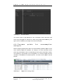
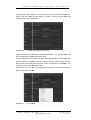
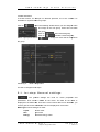
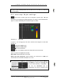
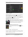
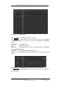
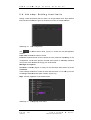
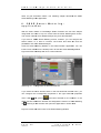
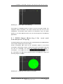
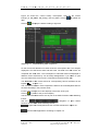
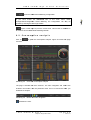
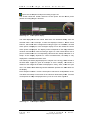
Smart Metering
Version 1.0
User Manual
Revision: 08.09.2011
I P A S
C o m B r i d g e
S t u d i o
E v o l u t i o n
Copyright Notice
The software and this documentation material is copyrighted and protected by
international treaties. ComBridge Studio Evolution and all other IPAS GmbH
product or services names are registered trademarks of IPAS GmbH. Other
brand and product names are also registered trademarks or trademarks of their
respective organization.
You may duplicate the documentation within the limits of the license agreement.
 2011 IPAS GmbH
P a g e
Version 1.0
2
I P A S
G m b H
Subject to change without notice
©
2 0 1 1
I P A S
C o m B r i d g e
S t u d i o
E v o l u t i o n
Content
1. Preface ............................................................................................................................. 4
3. Introduction ....................................................................................................................... 5
3.1. Energy meter.............................................................................................................. 5
3.2. Volumetric meter ........................................................................................................ 6
4. CBSE Smart Metering (SM) ............................................................................................. 7
4.1. Configuration of process points ................................................................................. 8
4.2. Process points for consumption analysis ................................................................. 10
5. Smart Metering Setup ..................................................................................................... 12
5.1. 1st step: General settings ........................................................................................ 13
5.2. 2nd step: Style settings ............................................................................................ 15
5.3. 3rd step: Load definition ........................................................................................... 16
5.4. 4th step: Setting load limits ...................................................................................... 18
6. CBSE Smart Metering-application .................................................................................. 20
6.1. CBSE Smart Metering Lite: cost and consumption display ..................................... 21
6.2. Consumption analysis .............................................................................................. 23
6.3. Load analysis ........................................................................................................... 26
6.4. Comparative analysis ............................................................................................... 28
7. Additional meter licenses ................................................................................................ 30
8. List of figures .................................................................................................................. 31
I P A S
G m b H
©
2 0 1 1
Subject to change without notice
P a g e
3
Version 1.0
I P A S
1 .
C o m B r i d g e
S t u d i o
E v o l u t i o n
P r e f a c e
This user manual outlines the functions of the ComBridge Studio Evolution Smart
Metering Module. A basic version of the module enabling simple analysis of up to
3 meters is part of the ComBridge Studio Evolution Basic Server delivery
package. This basic version can be extended by purchasing a ComBridge Studio
Evolution Smart Metering License. Then an additional two meters, i.e. a total of 5
meters, can be analysed. The type of meter used is independent of the license.
This manual describes the configuration and analysis of the ComBridge Studio
Evolution Smart Metering Module. The license can be obtained directly from
IPAS GmbH Duisburg (www.ipas-products.com) and installed on the server at
any time.
Order number:
Smart Metering Module
P a g e
Version 1.0
4
63102-32-10
I P A S
G m b H
Subject to change without notice
©
2 0 1 1
I P A S
3 .
C o m B r i d g e
S t u d i o
E v o l u t i o n
I n t r o d u c t i o n
At a time when the operation costs of a building are to a large extent determined
by its energy costs, applications as well as methods and concepts for usage
optimisation are becoming increasingly important.
To assess usage and consumption, meters are required which analyse
performance, volume or amount of heat and then transmit that data. Often a
pulse signal is used to denote a unit of consumption. The pulses emitted are
counted and multiplied by the unit. However, the market also offers meters which
provide the metered data in a specific data format.
This manual only deals with meters that provide data in the form of KNX
communications objects.
In principle, other data formats can also be processed. In this case, please
discuss the processing options with IPAS GmbH.
The theoretical concept of each type of meter is described below:
3.1. Energy meter
Energy meters measure electric power or electrical energy. Electric power is the
product of electrical potential difference and current:
P [W] = U [V] * I [A]
P is the electric power - the unit of measurement is Watts [W],
U is the electrical potential difference or electric tension – the unit of
measurement is Voltage [V],
I is the electric current - the unit of measurement is Amps [A].
Energy meters detect the voltage of an electronic device and measure the
current running through the device. The electric power is calculated from these
measurements.
Electrical potential difference, current and time multiplied by each other are
defined as electrical energy:
W [Ws] = U [V] * I [A]* t [s]
W is the electrical energy (in Joules, [Ws])
U is the electrical potential difference or electric tension, (in Volts [V])
I is the electric current, (in Amps, [A])
I P A S
G m b H
©
2 0 1 1
Subject to change without notice
P a g e
5
Version 1.0
I P A S
C o m B r i d g e
S t u d i o
E v o l u t i o n
t is the time (in seconds, [s])
When measuring energy consumption in the area of electrical engineering, the
unit kWh (kilowatt-hour) is most commonly used.
−7
1 kWh = 3.600.000 Ws, 1 Ws ≈ 2,778·10
kWh.
Energy meters are typically calibrated in kWh.
KNX – energy meters can have objects for active power per phase, total active
power and energy (meter reading). Electromechanical induction meters often
have a one pulse output. A pulse output corresponds to a certain amount of
energy passing through the meter. This amount is displayed on the meter.
For KNX energy meters there are two different types:
A: Pulse meter – the energy value is emitted via a pulse signal (e.g. S0-Bus). A
KNX node calculates the energy and power values from the number of pulses
and sends these onto the bus.
B: KNX – meter: The meter calculates power and energy and transmits the
results directly to the communication object.
The type of metering can influence the measured values: A read command for a
KNX meter tends to always result in accurate values as the measured value is
saved on the communications object until a new value is calculated. For a pulse
meter measured values, especially energy values, may be invalid. This is
because power is multiplied with a time unit. If a read command occurs within a
particular time interval, it could be that the value is found to be 0 as the energy
calculations have not yet been completed. This can happen especially in cases
where poling occurs cyclically.
3.2. Volumetric meter
Volumetric meters are used to measure gas or water consumption. To calculate
a volume, the cross-sectional area is required for the volumetric meter. A pulse
signal is emitted depending on the flow. The volume is hence calculated as
follows:
V = A * number of pulses
V is the volume
A is the cross-sectional area
Number of pulses.
As opposed to electrical energy, the pulse signal for the calculation of volume is
P a g e
Version 1.0
6
I P A S
G m b H
Subject to change without notice
©
2 0 1 1
C o m B r i d g e
I P A S
S t u d i o
E v o l u t i o n
time-independent. The number of pulses alone corresponds to the current flow.
The volumetric meter can usually be used for both gas and water.
When importing ETS communication objects (data points in CBS Evolution),
please ensure that the correct data format is defined for a data point. You can
use the data and process point mask to set both data point types (DPT) and subtypes (SubDPT). Please see the data sheet or the corresponding application
program description for the correct data point types and units of measurement.
With its ComBridge Studio Evolution Smart Metering Module (CBSE Smart
Metering) IPAS makes it possible to record, display and analyse the consumption
data of a building. The Smart Metering Module is the basis for professional
energy management, which IPAS offers individually and specified to customer
demands.
The CBSE Smart Metering is configured with the CBSE Editor and loaded as an
application in the CBSE visualisation. The CBSE Smart Metering can record data
of KNX electricity, gas and water meters. Under certain conditions data can also
be read from other systems.
The recorded data is saved as process points in a data base and can be
retrieved at any time.
To configure the CBSE Smart Metering Module a configured CBSE Server with
the corresponding license is required.
4 .
C B S E
S m a r t
M e t e r i n g
( S M )
CBS Evolution offers two versions of the SM Module. The CBSE Basic Version
includes the SM Module Lite without any extra license for up to 3 meters.
The CBSE SM Module analyses consumption data such as electrical energy or
water and gas consumption. A price per unit can be assigned to the consumption
data so that costs can be directly calculated depending on usage. The CBSE SM
Module Lite presents the data of all 3 meters either in bar or pie chart format. A
CBSE SM Module license extends the number of meters from 3 to 5. In addition,
the consumption data can be analysed in greater detail so that weekly, monthly
and annual estimates can be calculated depending on current usage. In addition,
the contribution of individual loads to the total consumption can be displayed.
Based on the data saved, different observation periods can also be compared
with each other.
The configuration of the SM Module is the same for both versions. The SM
Module obtains the required data from the data base. Use the process point
editor to determine whether you would like to save the data in the data base.
I P A S
G m b H
©
2 0 1 1
Subject to change without notice
P a g e
7
Version 1.0
C o m B r i d g e
I P A S
S t u d i o
E v o l u t i o n
Three steps are required to configure the SM Module:
1:
Configuration
onfiguration of all required process points:
Use CBSE Editor for this configuration.
2:
Meter configuration:
Use CBSE Editor or the application for this configuration.
3:
Data
ata display:
The data is displayed in the application and loaded via a CBSE function.
f
(
see chapters 5.8.3.1 and 6.6)
4.1. Configuration of process points
CBS Evolution communicates with connected systems via process points. In the
simplest case the
he basic information from a data point corresponds to the
parameters of a process point. For special functions, a process point can be
individually configured or even newly created.
By default, data is not saved in the data base. You therefore need to configure
the required process points accordingly.
Click on the left-hand
hand side menu process points to display the existing process
points.
Abbildung 1:
Process points display
Double-click
click on a process point to open its configuration window. Figure 2 shows
such a window.
P a g e
Version 1.0
8
I P A S
G m b H
Subject to change without notice
©
2 0 1 1
I P A S
Abbildung 2:
C o m B r i d g e
S t u d i o
E v o l u t i o n
Configuration
onfiguration of a process point
Click on PP log to open the window shown in figure 3.
3
Abbildung 3:
PP log
To save the data of the process point in the data base, you need to tick the It
logs box. To analyse the data in the SM Module
e you should also tick the
Interpolate box. Use
to save the settings for the process point.
PP auto control defines an individual load both when switched on and off.
Save value activates the function, Value ON and Value OFF describe the
current status, Consumption describes the load in [W].
Press
to accept the settings.
The events are analysed in the CBSE Smart Metering Module.
I P A S
G m b H
©
2 0 1 1
Subject to change without notice
P a g e
9
Version 1.0
I P A S
C o m B r i d g e
Abbildung 4:
S t u d i o
E v o l u t i o n
PP auto control
The electric power in [W] displayed in the consumption field is the load used
when the process point is switched on. When using CBSE Smart Metering,
Metering this
figure can be seen as a percentage of the total consumption.
4.2. Process
analysis
points
for
consumption
Before analysing consumption data in the Smart Metering Module, please check
which metered values are available. For example, if a meter only offers active
power per phase and no total, corresponding process points need to be created.
The following is an example of the configuration of a virtual process point that
calculates a total based on individual phases. The total is then edited in the SM
Module.
Abbildung 5:
P a g e
Version 1.0
1 0
Obje
Objects
of an energy meter
I P A S
G m b H
Subject to change without notice
©
2 0 1 1
I P A S
C o m B r i d g e
S t u d i o
E v o l u t i o n
Figure 5 shows the objects of an energy meter that only offers active power per
phase. Use the CBSE process points to create a virtual process point that
calculates the sum of the phases.
Abbildung 6:
Process point Total Active Power
Figure 6 shows the process point SumOfPhases(Ipas). The process point has
been assigned three individual power phases.
phases
Like the individual
ividual ones, the process point SumOfPhases(Ipas)
S
contains the data
point type DPT 14:4 Byte fload and the SubType 56: DPT_Value_Power. Use the
logic function OR to link the data points,
points which corresponds to an addition.
ddition. The
result is the sum of all individual
indivi
phases.
Alternatively, you can enter the mathematical formula in the Receive Function
Fun
field to generate the addition.
Abbildung 7:
I P A S
PP Function
ction
G m b H
©
2 0 1 1
Subject to change without notice
P a g e
1 1
Version 1.0
I P A S
C o m B r i d g e
S t u d i o
E v o l u t i o n
Click into the Receive Function field with the right mouse button to select the
data points from the menu and connect them with a “+“. The result is again the
total power.
Process
cess points that have been saved in the data base, can be recognised from
the data base symbol in the list of process points
.
You can also add individual values within the SM configuration (
chapter
4: SM Setup).
5 .
S m a r t
M e t e r i n g
S e t u p
The configuration of the meters is the same for CBSE
SM Lite and CBSE SM and only depends on the
number of meter licenses. Open the CBSE SM
configuration
in
CBSE
Editor
with
Modules/Consumption Control.
Abbildung 8:
Configuration
onfiguration Smart Metering
Figure 8 shows the configuration
co
screen. The total number of meter licenses is
displayed in the top left hand corner.
In this example a maximum of 10 licenses can be
configured.
The already configured meters are listed on the left
hand side of the window.
window On the right hand side, groups and meters can be
P a g e
Version 1.0
1 2
I P A S
G m b H
Subject to change without notice
©
2 0 1 1
C o m B r i d g e
I P A S
S t u d i o
E v o l u t i o n
created and edited.
If several meters,, for example on different premises, are to be created it is
advisable to organise them into groups.
Click on
to open the following window where you can assign a name
and image to the new group. Press save to create
the group.
Click on
to edit a selected group.
Click on
Select a group and click on
to delete a selected group.
to configure a meter that is assigned to
the group.
Abbildung 9:
Meter configuration
A meter is configured in 4 steps:
steps
5.1. 1st step: General settings
: The general settings are used for meter properties and
parameters. First choose a name for the meter. The data for the meter is
displayed in the detail view. So that the correct meter data can be identified, you
need to give the meter a Short-ID. This ID is displayed on all screens.
Meter type: Choose the type of meter.
meter
Liquid:
water meter
Gas:
gas meter
Energy:
ele
electrical
energy meter
I P A S
G m b H
©
2 0 1 1
Subject to change without notice
P a g e
1 3
Version 1.0
I P A S
C o m B r i d g e
Active power: click on the
S t u d i o
E v o l u t i o n
symbol to choose the process point for active
power in [W].
Some meters on the market only provide power readings for individual phases.
ComBridge Studio Evolution can calculate the total active power from the
individual phases and make these calculations available to the Smart Metering
Module (
see chapter 3.2).
Alternatively
ely you can calculate the active power in the general meter
configuration mask.
Abbildung 10:
Calculating active power
In figure 10, three process points for individual phases
hases have been selected with
.
By
clicking
on
the
process
point
1161:SumOfPhases has been created which calculates the active power by
adding the three individual phases together. This process point can also be used
in other elements and can be selected from the list of available process points.
The unit for active power always has to be [W]. Should the process point provide
another unit, it has to be converted in the function field of the process point.
Active energy: Click on
to select the process point for energy in KWh.
KWh If the
process point provides the energy only in [Ws], it has to be converted in the
function field of the process point.
point
KNX meter manufacturers do not use uniform data formats for active power and
energy. Active power is often provided in the format
f
DPT 14: 4 Byte Float,
Float SDPT
56: Value Power and energy in the format DPT 14: 4 Byte Float, SDPT 31: Value
Energy or DPT 12: 4 Byte Unsigned, SDPT 1: 4 Byte Ucount.
Please refer to the manufacturer‘s data sheet for the correct data type and use
this for the respective data and process points.
Price for 1 KWh: Sets the price for 1 KWh. At present the Smart Metering
Module cannot consider base rates or subscriber’s
subscri
rental for a meter.
Use
P a g e
Version 1.0
to save the settings.
settings
1 4
I P A S
G m b H
Subject to change without notice
©
2 0 1 1
I P A S
C o m B r i d g e
S t u d i o
E v o l u t i o n
For gas or water meters, please use the units m³/h or l³/h and l³ or m³ for
f flow
and consumption.
5.2. 2nd step: Style settings
: Each meter or meter type can be assigned a specific style.
style The style
determines, for example, the graphical display of a usage or its threshold values.
Figure 11 shows different styles for different types of meters.
Abbildung 11:
Style view
In figure 11 the energy style has been selected and assigned to the meter
Energie_IP.
copies the selected style.
style
deletes the selected style.
opens the Style Editor.
adds a new style and opens the Style Editor at the same time.
Figure 12 shows the Style Editor window.
window
Style name: defines the name of the style
Show units and show price:
price Select whether you would like to display the
results either in the unit of consumption or in cost.
Use Configuration/Configuration
onfiguration Smart Metering to select the required currency.
currency
Use Name to choose an individual name
for the Smart Metering configuration
onfiguration. If
you
tick
the
Password
box
box,
the
configuration can also be opened on-line
on
by using the Editor log-in
in details.
I P A S
G m b H
©
2 0 1 1
Subject to change without notice
P a g e
1 5
Version 1.0
I P A S
C o m B r i d g e
Abbildung 12:
S t u d i o
E v o l u t i o n
Style Editor
Show data tips: When the mouse hovers over a node in the consumption
analysis, the corresponding value is displayed. (
see chapter 5).
Show limits, Max.
ax. monthly money expected: If you tick this box, the value
defined in the Max. monthly money expected field, is displayed in the overview of
the consumption analysis. (
chapter 5). The value is adjusted to the
respective display, i.e. day, week or year.
Default colour: Colour for the display of the active power curve.
curve
Max/Min value: Sets the scaling of the online display of the consumption
analysis (
chapter 5). On the display the measuring range is scaled to the
range between min.
min value and max. value. In addition the
measuring range can be split into percentages, with the
resulting sections being displayed
displayed in different colours.
Abbildung 13:
Online display of the consumption analysis
Click on the slider to divide the sections into percentages [%].
Click on a colour field
fiel to select the colour. Press
to save
the settings.
settings
5.3. 3rd step: Load definition
This window is used to relate individual loads to a total load. To use this
application, a load has to be controlled via a process point that has been
configured according to chapter 3.1, figure 4.
P a g e
Version 1.0
1 6
I P A S
G m b H
Subject to change without notice
©
2 0 1 1
I P A S
Abbildung 14:
C o m B r i d g e
S t u d i o
E v o l u t i o n
Load overview
Figure 14 shows the 3 activated loads H1, H2 and H3
Use
to select further process points that have been configured
according to chapter 3.1.
3.1 Figure 15 shows the corresponding configuration
window.
Load name:
describes the load
Load:
selected process point
Value ON:
shows the status of the load. The corresponding load is entered
in the Consumption field.
field
Value OFF:
shows the unloaded status of the load
In figure 15 the process point H1 has been assigned a load of 250 W for the ON
status.
Abbildung 15:
Use
Adding/editing a process point for load observation
to edit configured process points and open the window shown in
figure 15 above.
I P A S
G m b H
©
2 0 1 1
Subject to change without notice
P a g e
1 7
Version 1.0
I P A S
C o m B r i d g e
S t u d i o
E v o l u t i o n
5.4. 4th step: Setting load limits
Setting a load limit means that an alarm can be generated when a pre-defined
pre
limit has been exceeded.
exceeded Figure 16 shows an overview of configured limits.
limits
Abbildung 16:
Use
Limit configuration
to define further limits.
limits Figure 17 shows the limit configuration
window.
Limit name: defines the name of a limit
Linked to: defines the link to the load that is to be observed. Depending on the
configuration,
n, one or more phases, the total active power or added up individual
ones (in the case of electrical energy) can be observed.
Message: Message title
Condition: Condition (higher or lower) for the threshold value that is set under
Threshold.
These settings are used to create an alarm with the name GesamtWirk_IP in the
ComBridge
e Studio Evolution alarm module. (Figure 18).
Style: sets the properties of the threshold line.
line
Abbildung 17:
P a g e
Version 1.0
1 8
Configuring a limit value
I P A S
G m b H
Subject to change without notice
©
2 0 1 1
I P A S
Abbildung 18:
C o m B r i d g e
S t u d i o
E v o l u t i o n
Limit value alarm in the CBSE alarm module
Figure 18 shows the alarm GesamtWirk_IP, which CBSE has automatically
created from the definitions above. In the above definitions (figure 17), a link to
active power was created which means that the process point for active power
(in the example 1087:GesamtWirk_IP)
1087:Ge
is observed. The alarm conditions are
also obtained from the definition of the limit value (in
in the example:
example
GesamtWirk_IP > 2345 W, see figure 17). In addition the message ‘Max
Max Power is
overloaded’ appears in the Message field of the CBSE alarm module
e (see figure
17). Figure 19 shows the corresponding configuration window, for example to
forward the message as an e-mail.
e
Abbildung 19:
Alarm forwarding in the CBSE alarm module/message
This 4th step concludes the configuration of a meter (in this
th case an energy
meter) in the CBSE Smart Metering Module.
Modul The configuration steps are the
I P A S
G m b H
©
2 0 1 1
Subject to change without notice
P a g e
1 9
Version 1.0
I P A S
C o m B r i d g e
S t u d i o
E v o l u t i o n
same for gas and water meters. The following chapter describes the CBSE
Smart Metering online application.
application
6 . C B S E S m a r t
a p p l i c a t i o n
M e t e r i n g -
With the basic version of ComBridge Studio Evolution the user can analyse
usage data and costs of up to 3 meters with the Smart Metering Lite version.
This version offers a more detailed analysis only as a demonstration.
If you have a CBSE Smart Metering license, however, you can analyse two
further meters, i.e. a total of 5 meters. The license also offers the user the
possibilities of a more detailed analysis.
Load the Smart Metering Module
Modul in the CBS Evolution application. You can
insert a menu element in the desktop menu to start
sta the Smart Metering Module.
Modul
Figure 20 shows a desktop
deskt with such a menu element.
Abbildung 20:
Configuration
onfiguration of SM menu element
If you select the menu element Demo in the left hand-side
side function menu, you
can configure the corresponding properties in the right hand-side
side properties
menu. With
the symbol
has been selected for the element. In the
CBSE function window the element was assigned the function 8: Smart Metering
via
. Clicking on the element now opens the application in online mode.
Figure 21 shows the start screen of the Smart Metering Module.
Module
P a g e
Version 1.0
2 0
I P A S
G m b H
Subject to change without notice
©
2 0 1 1
I P A S
Abbildung 21:
C o m B r i d g e
S t u d i o
E v o l u t i o n
Start screen Smart Metering
The number of configured meters is shown in the top left hand corner. The
configured meters are listed in the folder structure that was set up in the
configuration. At least one meter needs to be selected to carry out further
analysis. If you select several meters, they can all be analysed in the following
applications.
6.1. CBSE Smart Metering
consumption display
Lite:
cost
and
The Smart Metering Lite Version that is part of CBS Evolution ServerBasic allows
for the simple analysis of up to three meters.
meters
Current consumption and costs can be calculated. Based on the current
consumption, estimates for weekly, monthly and annual consumption and costs
can also be calculated. The results are updated with each change in
consumption. If you press one of the
b
buttons,
the consumption and costs for the selected meters are displayed in a pie chart
according to figure 22 below.
below
Abbildung 22:
I P A S
isplay of current weekly consumption
Display
G m b H
©
2 0 1 1
Subject to change without notice
P a g e
2 1
Version 1.0
C o m B r i d g e
I P A S
S t u d i o
E v o l u t i o n
Figure 22 shows the current weekly consumption costs for the meters
Energie_IP, KM_Water, KM_Energy und HE_Water.
HE_Water Click on
to update the
data.
Click on
to display the data according to figure 23.
Abbildung 23:
Smart Metering data comparison
On this screen two different bar charts show the consumption data. The analysis
displayed is for the current week and last week. The data
ata from each meter are
compared with each other. The consumption of individual meters is displayed in
different colours so that they can be easily distinguished. If you switch to year
view,, the data for the
th current year is compared to the data for last year.
year
The Short-IDss of the meters and their corresponding colours are listed in the
legend (
chapter 4.1).
The “comparison
comparison details“
details chart compares the data for each weekday with data for
the same weekday in the previous week.
For the yearly analysis, this view displays each month of the year.
Click on
to return to the pie chart display.
The functions described above are all part of the CBS Evolution
on Smart Metering
license.
Use the
navigation to open further
functions of the CBSE Smart Metering Module.
opens the consumption and cost overview described in chapter 5.1.
5.1
opens further applications according to chapter 5.2.
P a g e
Version 1.0
2 2
I P A S
G m b H
Subject to change without notice
©
2 0 1 1
I P A S
C o m B r i d g e
S t u d i o
E v o l u t i o n
opens the CBSE Smart Metering configuration.
c
If
you
have
ticked
the
Password
box
in
the
main
menu
under
Configuration/Configuration
onfiguration Smart Metering,
Metering, the configuration can only be
opened by entering the user login details.
opens a PDF report
eport to print the current view. This function is available in
all versions of the CBSE Smart Metering Module.
Modul
6.2. Consumption analysis
Click on
to open the consumption analysis. Figure 24 shows the page
overview.
Abbildung 24:
Overview consumption analysis
The page is divided into three sections. The main navigation and menus are
located in the header. Use the pull-down
p
menu Select to choose the meter you
would like to analyse.
Abbildung 25:
Menus and main navigation
refreshes the view.
I P A S
G m b H
©
2 0 1 1
Subject to change without notice
P a g e
2 3
Version 1.0
I P A S
C o m B r i d g e
S t u d i o
E v o l u t i o n
opens the consumption analysis according to figure 24.
The section below the header shows the active power and the active power
phases according to figure 26 below.
Abbildung 26:
Active power display
The data displayed here are online data which are obtained directly from the
selected meter. In
n the example,
example 4 charts are displayed: Phase 1, Phase 2 and
a
Phase 3, which have been configured according to figure 10. In addition, the total
active power is displayed.
displayed In the analogue display next to the charts,
charts the current
active power is displayed. The display scale corresponds to the range between
minimum and maximum value according to figure 12.
12 If the mouse hovers over a
point of measurement, the corresponding value and time stamp are shown in a
tooltip. As the display depends on current measurements, the tooltip
tool
is only
displayed if a valid value has been sent.
The bottom part of the page displays an analysis
analysis of the energy values saved in
i
the data base. Figure 27 gives an example of such a display. The section is
divided in such way that the data are displayed in a day, week, month and year
view. The CBSE Smart Metering Module
Module database provides the data tables for
the display.
Each analysis includes a current consumption chart and a trend/prevision
prevision chart.
cha
The tables are built up on the basis of the narrower observation period. First the
consumption for today is displayed hour by hour in a bar chart. Figure 27
Abbildung 27:
P a g e
Version 1.0
2 4
Consumption analysis
I P A S
G m b H
Subject to change without notice
©
2 0 1 1
I P A S
C o m B r i d g e
S t u d i o
E v o l u t i o n
was created at 4pm,, so that the accumulated consumption for the day is only
displayed until 4pm. Consumption was significantly lower during night hours.
Around 8 am, computers, lights and other devices were switched on so that the
consumption increased. The monthly maximum value that is defined according to
figure 12 is displayed
played as a red line in all charts. In the weekly consumption view,
the values for each weekday are displayed. The chart was created on a
Wednesday (around
around 4pm).
4pm As the consumption for Wednesday was not yet
complete, the consumption is much lower than that on Monday and Tuesday.
th
The display of month and year show that it was created on May 4 . The CBSE
Smart Metering Module calculates the current consumption and the average
value for a day, week, month and year.
These values are displayed in the
prevision tables and updated depending on current usage. In addition, CBSE
Smart Metering calculates the estimated consumption at the end of the
observation period. Click on
in the top right hand corner of each chart title to
open a full screen view according to figure 28.
28 In figure 28, the bar in the middle
shows the current consumption up to the point the chart was created. In the
example the currently accumulated consumption
consu
is 93.57 KWh or 18.71
71 €. This
means that the average consumption per day is 31.19 KWh or 6.24 €. Based on
the current consumption, consumption for the week is estimated to be 239.6
KWh or 47.92 €. Should
hould the consumption data change, the estimate will
wil also
change. This means that consumption estimates and costs for day, week, month
and year can be calculated at any time based on current usage and any changes
can be taken into consideration when trying to estimate costs for the year or
another period ahead.
Abbildung 28:
Click on
I P A S
Consumption analysis: Prevision
in the top right hand corner to return to the overall view.
G m b H
©
2 0 1 1
Subject to change without notice
P a g e
2 5
Version 1.0
I P A S
C o m B r i d g e
S t u d i o
E v o l u t i o n
6.3. Load analysis
Click on
in the selection menu to open the load analysis according to figure
29 below. This application can be used to display the proportion of different loads
in relation to the total load and to calculate how they influence consumption and
costs. To be able to use this application, the corresponding process points need
to be configured according to chapters 3.1 and 4.3. The process points
configured this way are used as active elements in the load analysis as shown in
figure 30.
Abbildung 29:
oad analysis
Load
Abbildung 30:
Overview load analysis
P a g e
Version 1.0
2 6
I P A S
G m b H
Subject to change without notice
©
2 0 1 1
I P A S
C o m B r i d g e
S t u d i o
E v o l u t i o n
In
n the example the three loads H1, H2, H3 have been defined. The pie chart in
the top right hand corner shows the total consumption and how each load
contributes to it. If you click on the individual pieces, they are pulled out slightly
as shown
own in figure 31 below.
If you hover over one of the pieces with
h the mouse,
mouse
its percentage of the total consumption and the
current value (in brackets) are displayed. In the
example, the percentage of H1 of the total
consumption is 7.9%.
Abbildung 31:
Current load distribution
As before the CBSE Smart Metering Module
Module calculates daily, weekly, monthly
and annual consumption as well as the corresponding future estimates. Figure
32 shows the weekly consumption and estimate based on the details in figure 30.
Abbildung 32:
Load analysis
nalysis based on details in figure 30
If all three loads H1, H2, H3 are switched
d on, the cost estimate for the current
week is 12.92 €.
This calculation is updated immediately if the load
changes.
For
example,
if
H2
is
switched
off,
consumption and costs for the week are calculated as
in figure 33.
Abbildung 33:
I P A S
Load
oad analysis if load changes
G m b H
©
2 0 1 1
Subject to change without notice
P a g e
2 7
Version 1.0
I P A S
C o m B r i d g e
S t u d i o
E v o l u t i o n
The new calculation means that the cost estimate falls to 7,64 €.
This application can be used to simulate measures that can help to lower energy
costs.
6.4. Comparative analysis
The results from the consumption
consumption and load analysis are saved in
i the CBSE
Smart Metering data base. In addition to the current and estimated consumption
plus cost developments, long-term
long term observation can be important to assess the
effectiveness of certain measures. For this purpose the CBSE Smart Metering
Module
e makes it possible to compare observation periods (days, weeks, months,
years). Two observation periods
perio can be compared to each other. Click on
in
the menu to open the window shown in figure 34 below.
Abbildung 34:
Selecting the observation range
Beginning first range and Beginning second range set the date for the
beginning of the periods
period that are to be compared. According to figure 34, the first
range starts on 1 July 2011 and the second range on 1 August 2011. In this case
the
he length of the observation period is 30 days starting on the above dates (you
can choose between days, weeks, months and years). The result is displayed in
figure 35. Each
ach day is represented by a bar. The height of the bar corresponds to
the daily consumption. No data is available for the first six days of the first range.
range
The second range is complete. Select a day to show the consumption
consu
data.
Double-click on the day to show the hourly consumption as shown in figure 36.
The comparison in figure 35 shows the consumption to be relatively constant.
constant
Consumption is lower at weekends.
weekends The analysis showss that a constant load of
22 KWh is required
equired on average every day.
P a g e
Version 1.0
2 8
I P A S
G m b H
Subject to change without notice
©
2 0 1 1
I P A S
C o m B r i d g e
S t u d i o
E v o l u t i o n
Abbildung 35:
Comparing selected observation ranges
Abbildung 36:
Display of daily consumption after double-click
double click on a selected day
In order to compare the differences directly with each other, you can also drag &
drop individual days into the section “comparison“ on the right hand side. Figure
37 gives an example of a resulting pie chart.
I P A S
G m b H
©
2 0 1 1
Subject to change without notice
P a g e
2 9
Version 1.0
I P A S
C o m B r i d g e
Abbildung 37:
S t u d i o
E v o l u t i o n
Dire comparison of two days in the observation range
Direct
In the example the 20th day of each month is compared with
w th each other. In July
consumption was 10% higher than in August.
This application can be used to monitor and evaluate the effectiveness of any
energy saving measures undertaken.
7 .
Ad d i t i o n a l
m e t e r
l i c e n s e s
Summary of CBSE modules:
modules
Software
Function
Order number
CBS Evolution Server
Includes Smart Metering
63102
63102-32-01
Lite for 3 meters
CBS Smart Metering
Includes 2 further meter
63102
63102-32-10
licenses
CBS SM counter extension
5 additional licenses
63102
63102-32-52
The additional licenses can be added at any time.
time For training courses about
CBSE and
nd CBSE SM please go to www.ipas-products.com.
P a g e
Version 1.0
3 0
I P A S
G m b H
Subject to change without notice
©
2 0 1 1
I P A S
8 .
L i s t
o f
C o m B r i d g e
S t u d i o
E v o l u t i o n
f i g u r e s
Abbildung 1:
Process points display.................................................................. 8
Abbildung 2:
Configuration of a process point .................................................. 9
Abbildung 3:
PP log ........................................................................................... 9
Abbildung 4:
PP auto control ........................................................................... 10
Abbildung 5:
Objects of an energy meter ........................................................ 10
Abbildung 6:
Process point Total Active Power .............................................. 11
Abbildung 7:
PP Function ................................................................................ 11
Abbildung 8:
Configuration Smart Metering .................................................... 12
Abbildung 9:
Meter configuration ..................................................................... 13
Abbildung 10:
Calculating active power ......................................................... 14
Abbildung 11:
Style view ................................................................................ 15
Abbildung 12:
Style Editor ............................................................................. 16
Abbildung 13:
Online display of the consumption analysis............................ 16
Abbildung 14:
Load overview ......................................................................... 17
Abbildung 15:
Adding/editing a process point for load observation ............... 17
Abbildung 16:
Limit configuration ................................................................... 18
Abbildung 17:
Configuring a limit value ......................................................... 18
Abbildung 18:
Limit value alarm in the CBSE alarm module ......................... 19
Abbildung 19:
Alarm forwarding in the CBSE alarm module/message ......... 19
Abbildung 20:
Configuration of SM menu element ........................................ 20
Abbildung 21:
Start screen Smart Metering ................................................... 21
Abbildung 22:
Display of current weekly consumption .................................. 21
Abbildung 23:
Smart Metering data comparison ........................................... 22
Abbildung 24:
Overview consumption analysis ............................................. 23
Abbildung 25:
Menus and main navigation .................................................... 23
Abbildung 26:
Active power display ............................................................... 24
Abbildung 27:
Consumption analysis............................................................. 24
Abbildung 28:
Consumption analysis: Prevision ............................................ 25
Abbildung 29:
Load analysis .......................................................................... 26
Abbildung 30:
Overview load analysis ........................................................... 26
Abbildung 31:
Current load distribution.......................................................... 27
Abbildung 32:
Load analysis based on details in figure 30 ........................... 27
Abbildung 33:
Load analysis if load changes ................................................ 27
Abbildung 34:
Selecting the observation range ............................................. 28
Abbildung 35:
Comparing selected observation ranges ................................ 29
Abbildung 36:
Display of daily consumption after double-click on a selected
day
29
Abbildung 37:
I P A S
Direct comparison of two days in the observation range........ 30
G m b H
©
2 0 1 1
Subject to change without notice
P a g e
3 1
Version 1.0
I P A S
C o m B r i d g e
P a g e
3 2
Version 1.0
S t u d i o
E v o l u t i o n
I P A S
G m b H
Subject to change without notice
©
2 0 1 1