Download Design of a Wearable Ultrasound System

Abstract
Ultrasound imaging is a safe and powerful tool for providing detailed still and moving
images of the human body. Most of today’s ultrasound systems are housed on a
movable cart and designed for use within a clinical setting, such as in a hospital or
doctor’s office.
This configuration hinders its use in locations lacking controlled
environments and stable power sources. Example locations include ambulances,
disaster sights, war zones and rural medicine.
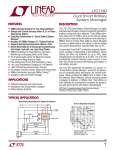
A wearable ultrasound system, in the form of a vest worn by a sonographer, has
been developed as a complete solution for performing untethered ultrasound
examinations. The heart of the system is an enclosure containing an embedded
computer running the Windows XP operating system, and a custom power supply.
The power supply integrates a battery charger, a switching regulator, two linear
regulators, a variable speed fan controller and a microcontroller providing an
interface for monitoring and control to the embedded computer. Operation of the
system is generally accomplished through the use of voice commands, but it may
also be operated using a hand-held mouse. It is capable of operating for a full day,
using two batteries contained in the vest.
In addition, the system has the capability to wirelessly share live images with remote
viewers in real-time, while also permitting full duplex voice communication.
An
integrated web-server also provides for the wireless retrieval of stored images,
image loops and other information using a web-browser.
ii
Preface
I would like to acknowledge the assistance of the Telemedicine and Advanced
Technology Research Center (TATRC) in providing invaluable resources throughout
the duration of this research. In addition, the diligent work and effort provided by the
Informatics staff and Army medical professionals at Madigan Army Medical Center
(MAMC) has helped to make this research a success.
The tutelage and mentoring provided by Professor Peder C. Pedersen and
Professor R. James Duckworth has been fundamental to the success of this work
and is greatly appreciated.
Also, the craftsmanship provided by Robert Boisse
contributed immensely to the quality and reliability of the final design.
iii
Table of Contents
1
2
3
4
5
Introduction .........................................................................................................1
1.1
Ultrasound Imaging Primer ..........................................................................3
1.2
Ultrasound Applications .............................................................................15
1.3
Portable Ultrasound ...................................................................................16
1.4
Motivation and Justification ........................................................................19
Wearable Ultrasound ........................................................................................21
2.1
Introduction to Wearable Ultrasound..........................................................21
2.2
Architecture................................................................................................22
2.3
Requirements ............................................................................................26
2.3.1
Enclosure Requirements ....................................................................27
2.3.2
Enclosure Connector Requirements ...................................................27
2.3.3
Power Supply Requirements ..............................................................28
2.3.4
Embedded Computer Requirements ..................................................29
2.3.5
Software .............................................................................................29
2.4
Development History..................................................................................30
Embedded Computing Platform ........................................................................33
3.1
Embedded Computer.................................................................................33
3.1.1
PC/104 Standards ..............................................................................33
3.1.2
Embedded Computer Selection ..........................................................35
3.1.3
IEEE 1394a Selection.........................................................................37
3.1.4
Hard Disk Drive Selection ...................................................................37
3.1.5
IEEE 802.11b/g Selection ...................................................................38
3.2
EDCM Integration ......................................................................................38
3.3
Enclosure Design.......................................................................................39
3.3.1
Internal Arrangement ..........................................................................43
3.3.2
Enclosure Connectors ........................................................................49
3.3.3
Enclosure Assembly ...........................................................................50
Power Supply and Management .......................................................................54
4.1
Justification ................................................................................................54
4.2
Introduction ................................................................................................56
4.3
Smart Battery System Manager .................................................................58
4.4
Li-Ion Rechargeable Batteries ...................................................................63
4.5
5V Switching Regulator..............................................................................66
4.6
Linear Regulators.......................................................................................70
4.7
SMBus to RS-232 Host Interface ...............................................................72
4.8
Fan Controller ............................................................................................78
4.9
Power Supply PCB Design ........................................................................80
4.10 IEEE 1394a Power Supply.........................................................................82
4.11 User Interface ............................................................................................83
Speech Recognition ..........................................................................................88
5.1
Background................................................................................................88
5.2
Implementation ..........................................................................................92
5.2.1
Speech Recognition Initialization ........................................................92
5.2.2
Speech Recognition Runtime .............................................................95
iv
5.3
User Interface ............................................................................................ 99
5.4
Terason Application Integration ............................................................... 103
5.5
Patient Information .................................................................................. 105
5.6
Array Microphone .................................................................................... 107
6 Remote Data Facilities.................................................................................... 108
6.1
Physical Layer ......................................................................................... 108
6.2
Transport Layer ....................................................................................... 109
6.3
Real-Time Transport Protocol.................................................................. 111
6.4
Real-Time Ultrasound Imaging ................................................................ 115
6.5
Voice Communications............................................................................ 123
6.6
Remote Administration ............................................................................ 125
7 Logging........................................................................................................... 129
7.1
Logging Method....................................................................................... 129
7.2
Logging Data Store.................................................................................. 131
7.3
Data Analysis........................................................................................... 137
8 System Integration.......................................................................................... 146
8.1
Hardware Integration ............................................................................... 146
8.2
Software Integration ................................................................................ 149
8.3
User Integration ....................................................................................... 151
9 Technical Performance................................................................................... 153
9.1
Battery Charger ....................................................................................... 153
9.2
5 V Switching Regulator .......................................................................... 163
9.3
Embedded Computing Platform Thermals............................................... 166
9.4
Speech Recognition ................................................................................ 168
9.5
Specifications .......................................................................................... 172
10
Clinical Usage and Value ............................................................................ 174
10.1 Applications ............................................................................................. 175
10.1.1 Telemedicine .................................................................................... 175
10.1.2 Disaster Relief .................................................................................. 176
10.1.3 Medical Transport............................................................................. 177
10.1.4 Rural Healthcare .............................................................................. 178
10.1.5 Military .............................................................................................. 178
10.2 Out-of-Box Experience ............................................................................ 179
11
Conclusion and Further Work ..................................................................... 182
References ............................................................................................................ 191
Appendix I – Bill of Materials.................................................................................. 194
Appendix II – Internal Cable Assemblies ............................................................... 198
Appendix III – External Cable Assemblies ............................................................. 205
Appendix IV – Schematics ..................................................................................... 209
Appendix V – PCB Layout ..................................................................................... 211
Appendix VI – Speech Recognition Grammar ....................................................... 214
Appendix VII – Database Schema ......................................................................... 216
Appendix VIII – Training Video Scripts................................................................... 218
v
Table of Figures
Fig. 1: Sample A-Mode Image [2]...............................................................................4
Fig. 2: Early B-Mode Ultrasound Machine [2].............................................................6
Fig. 3: Early B-Mode Ultrasound Image [3] ................................................................6
Fig. 4: M-Mode Ultrasound Image [4] .........................................................................7
Fig. 5: Pulsed Wave Doppler Ultrasound Image [4] ...................................................8
Fig. 6: Power Doppler Ultrasound Image [4] ..............................................................9
Fig. 7: Color Doppler Ultrasound Image [4] ..............................................................10
Fig. 8: 3D Volume Image [5].....................................................................................11
Fig. 9: Rendered 3D Volume Image [6] ....................................................................12
Fig. 10: 4D Ultrasound Image [7] .............................................................................13
Fig. 11: 4-2 MHz Convex Array Transducer [4] ........................................................14
Fig. 12: 10-5 MHz Linear Array Transducer [4] ........................................................14
Fig. 13: 10-5 MHz Phased Array Transducer [4] ......................................................14
Fig. 14: 3.5 MHz Ultrasound Image [8].....................................................................15
Fig. 15: 5 MHz Ultrasound Image [8]........................................................................15
Fig. 16: GE LOGIQ 9 [9]...........................................................................................16
Fig. 17: SonoSite 180 Plus [10]................................................................................17
Fig. 18: Example Portable Ultrasound Machines .....................................................18
Fig. 19: Terson 2000 SmartProbe ............................................................................22
Fig. 20: Head Mounted Displays ..............................................................................24
Fig. 21: Trackball Mouse ..........................................................................................24
Fig. 22: Block Diagram of WUC ...............................................................................25
Fig. 23: First Generation WUC .................................................................................30
Fig. 24: Second Generation Embedded Computer, Power Supply and Enclosure...31
Fig. 25: PC/104-Plus Board Stackup [21].................................................................34
Fig. 26: Lippert-AT Cool RoadRunner 4 [23] ............................................................36
Fig. 27: Advanced Digital Logic MSM855 [24]..........................................................36
Fig. 28: EDCM Enclosure.........................................................................................39
Fig. 29: EDCM PCB .................................................................................................39
Fig. 30: Embedded Computer Enclosure .................................................................40
Fig. 31: Enclosure Components ...............................................................................41
Fig. 32: Dimensioned Embedded Computer Enclosure Drawing .............................43
Fig. 33: Two Compartments of Enclosure ................................................................44
Fig. 34: Top Compartment of Enclosure...................................................................44
Fig. 35: CPU Board and IEEE 1394a Board Assembly ............................................46
Fig. 36: Power Supply and HDD Assembly ..............................................................47
Fig. 37: Two Internal Assemblies .............................................................................47
Fig. 38: EDCM Mounting in Enclosure .....................................................................48
Fig. 39: Complete Internal Assembly of Lower Compartment ..................................48
Fig. 40: Cable Strain Relief Alcove...........................................................................49
Fig. 41: Enclosure Connector Model ........................................................................50
Fig. 42: Step One of Assembling the Enclosure.......................................................51
Fig. 43: Step Two of Assembling the Enclosure.......................................................52
Fig. 44: Enclosure ....................................................................................................52
vi
Fig. 45: OceanServer Battery Charger and ATX Power Supply [28,29]................... 55
Fig. 46: 1/8 Brick DC-DC Converter [30].................................................................. 55
Fig. 47: Block Diagram of Power Supply.................................................................. 57
Fig. 48: Example Smart Battery system [32]............................................................ 59
Fig. 49: Power Path Switch...................................................................................... 62
Fig. 50: Inspired Energy NL2024A22 Rechargeable Li-Ion Battery ......................... 65
Fig. 51: Block Diagram of Smart Battery Pack [37] .................................................. 66
Fig. 52: Power Supply Reference Design [39] ......................................................... 68
Fig. 53: Output Voltage Adjustment of Linear Voltage Regulator............................. 71
Fig. 54: Power Supply SMBus Block Diagram ......................................................... 74
Fig. 55: Generic SMBus Topology [40] .................................................................... 75
Fig. 56: SMBus START and STOP Conditions [40] ................................................. 75
Fig. 57: SMBus Protocols ........................................................................................ 76
Fig. 58: Host SMBus Command Packet................................................................... 77
Fig. 59: Local Temperature Sensor Control Loop .................................................... 80
Fig. 60: Remote Temperate Sensor Control Loop ................................................... 80
Fig. 61: Populated Power Supply PCB .................................................................... 81
Fig. 62: Dashboard .................................................................................................. 84
Fig. 63: Power supply area of the Dashboard .......................................................... 84
Fig. 64: Low Battery Warning Indicator .................................................................... 86
Fig. 65: Power Supply Dialog Box............................................................................ 86
Fig. 66: Context Creation ......................................................................................... 93
Fig. 67: Speech Recognition System Runtime......................................................... 95
Fig. 68: Circular Buffer ............................................................................................. 96
Fig. 69: WPI Application Overview........................................................................... 98
Fig. 70: Push-To-Talk Button ................................................................................... 99
Fig. 71: Speech Recognition States....................................................................... 100
Fig. 72: Successful Recogntion of “live image” ...................................................... 101
Fig. 73: Poor Recognition of “power doppler” ........................................................ 101
Fig. 74: ASR Details Dialog Box ............................................................................ 102
Fig. 75: View Utterances Dialog Box...................................................................... 103
Fig. 76: Shutdown Dialog Box................................................................................ 105
Fig. 77: Shutdown Progress Dialog Box ................................................................ 105
Fig. 78: Patient Information Dialog Box.................................................................. 106
Fig. 79: Patient Information Header ....................................................................... 106
Fig. 80: Linear Array Microphone........................................................................... 107
Fig. 81: Linear Array Microphone Directional Sensitivity........................................ 107
Fig. 82: OSI Reference Model [43]......................................................................... 108
Fig. 83: RTP Network Stack................................................................................... 112
Fig. 84: Buffer Backed GUI .................................................................................... 119
Fig. 85: Lost Image Tile ......................................................................................... 119
Fig. 86: RID Without Client .................................................................................... 121
Fig. 87: RID With Client Connected ....................................................................... 121
Fig. 88: RID Client Connection Dialog Box ............................................................ 122
Fig. 89: RID Client Application ............................................................................... 122
Fig. 90: Web Server Home Page ........................................................................... 126
vii
Fig. 91: User's Guide on Web Server.....................................................................126
Fig. 92: Saved Images on Web Server...................................................................127
Fig. 93: Data Analysis Application Connection Dialog............................................138
Fig. 94: Database Analysis Application Database Menu ........................................139
Fig. 95: Database Analysis Application View Menu ...............................................140
Fig. 96: Database Analysis Application Filters Menu .............................................141
Fig. 97: Date Filter Dialog Box ...............................................................................141
Fig. 98: Database Analysis Program Utterance View.............................................142
Fig. 99: Database Analysis Program Word Occurrence View ................................143
Fig. 100: Database Analysis Program ASR Errors View ........................................144
Fig. 101: Temperatures View Plot ..........................................................................145
Fig. 102: Vest Front................................................................................................146
Fig. 103: Vest Back ................................................................................................146
Fig. 104: Vest Component Layout..........................................................................148
Fig. 105: Single Smart Battery Relative Charge Capacity vs. Time While Charging
...............................................................................................................................154
Fig. 106: Manufacturer Single Cell Charge Characteristics [37].............................155
Fig. 107: Single Smart Battery Charge Characteristics ..........................................156
Fig. 108: Single Smart Battery Relative Charge Capacity vs. Time While Discharging
...............................................................................................................................157
Fig. 109: Single Smart Battery Discharge Characteristics......................................157
Fig. 110: Smart Battery Charger Switching Regulator Providing 3 A (DC Coupled)
...............................................................................................................................160
Fig. 111: Smart Battery Charger Switching Regulator Providing 3 A (AC Coupled)
...............................................................................................................................161
Fig. 112: Smart Battery Charger Switching Regulator Providing 0.5 A (DC Coupled)
...............................................................................................................................162
Fig. 113: Smart Battery Charger Switching Regulator Providing 0.5 A (AC Coupled)
...............................................................................................................................163
Fig. 114: 5 V Switching Regulator with 35 W Load (DC Coupled)..........................164
Fig. 115: 5 V Switching Regulator with 35 W Load (AC Coupled) ..........................165
Fig. 116: 5 V Switching Regulator with No Load (DC Coupled) .............................166
Fig. 117: Temperature Testing ...............................................................................167
Fig. 118: Utterance Frequency...............................................................................169
Fig. 119: Average Utterance Confidence ...............................................................170
Fig. 120: Sonosite MicroMaxx [55] .........................................................................174
Fig. 121: Bag Based Ultrasound System................................................................189
Fig. 122: Cable Length Measurement ....................................................................198
Fig. 123: Cable Length Measurement Example .....................................................198
Fig. 124: Cable Length Measurement ....................................................................205
Fig. 125: Cable Length Measurement Example .....................................................205
Fig. 126: Top Silkscreen.........................................................................................211
Fig. 127: Top Copper .............................................................................................211
Fig. 128: Layer 2 Copper........................................................................................212
Fig. 129: Layer 3 Copper........................................................................................212
Fig. 130: Bottom Copper ........................................................................................213
viii
Fig. 131: Bottom Silkscreen (horizontally mirrored) ............................................... 213
Fig. 132: Database Schema .................................................................................. 217
ix
Table of Tables
Table 1: Component Terminology ............................................................................25
Table 2: Available CPUs for MSM855......................................................................36
Table 3: Properties of Delrin [27]..............................................................................42
Table 4: Power Requirements for WUC Components ..............................................57
Table 5: Power Requirements by Regulated Voltage...............................................58
Table 6: Characteristics of Commonly Used Rechargeable Batteries [36]...............63
Table 7: Attributes of Linear and Switching Regulators [38].....................................67
Table 8: SMBus Memory Map..................................................................................74
Table 9: SMBus Protocol Mnemonics ......................................................................76
Table 10: PCB Design Rules....................................................................................81
Table 11: Speech Recognition Engine Types ..........................................................88
Table 12: Chomsky Hierarchy ..................................................................................90
Table 13: WUC Application Defined Messages......................................................130
Table 14: MySQL Numeric Data Types..................................................................132
Table 15: MySQL Binary Data Types.....................................................................133
Table 16: MySQL String Data Types......................................................................133
Table 17: tblPackets Definition...............................................................................133
Table 18: tblIMessages Definition ..........................................................................134
Table 19: tblUtterance Definition ............................................................................134
Table 20: tblWords Definition .................................................................................135
Table 21: tblAudio Definition ..................................................................................135
Table 22: tblBattery Definition ................................................................................136
Table 23: tblCPUTemp Definition...........................................................................136
Table 24: tblErrors Definition..................................................................................137
Table 25: tblImages Definition................................................................................137
Table 26: Software Components............................................................................149
Table 27: Training Videos ......................................................................................152
Table 28: WUC Specifications................................................................................173
Table 29: Power Supply Bill of Materials ................................................................194
Table 30: Embedded Computer Bill of Materials ....................................................195
Table 31: Internal Cable Bill of Materials................................................................196
Table 32: External Cable Bill of Materials ..............................................................196
Table 33: Assembly Bill of Materials ......................................................................196
Table 34: Internal 802.11g Cable Assembly...........................................................199
Table 35: Internal Audio Cable Assembly ..............................................................199
Table 36: Internal Battery 1 Cable Assembly .........................................................199
Table 37: Internal Battery 2 Cable Assembly .........................................................200
Table 38: Internal Charger Cable Assembly...........................................................200
Table 39: Internal CMOS Battery Cable Assembly ................................................200
Table 40: Internal Fan Power Cable Assembly ......................................................201
Table 41: Internal HDD Cable Assembly................................................................201
Table 42: Internal IEEE 1394a Auxiliary Power Cable Assembly...........................201
Table 43: Internal IEEE 1394a Cable Assembly ....................................................202
Table 44: Internal Mouse Cable Assembly.............................................................203
x
Table 45: Internal MSM855 CPU Power Cable Assembly ..................................... 203
Table 46: Internal Power Switch Cable Assembly ................................................. 203
Table 47: Internal Temperature Probe Cable Assembly ........................................ 204
Table 48: Internal USB Cable Assembly................................................................ 204
Table 49: Internal VGA Cable Assembly................................................................ 204
Table 50: External VGA Cable Assembly .............................................................. 206
Table 51: External Audio Cable Assembly............................................................. 206
Table 52: External Mouse Cable Assembly ........................................................... 207
Table 53: External USB Cable Assembly............................................................... 207
Table 54: External Battery 1 Cable Assembly........................................................ 207
Table 55: External Battery 2 Cable Assembly........................................................ 208
Table 56: External Charger Cable Assembly ......................................................... 208
Table 57: MySQL and ODBC Data Type Mappings............................................... 216
xi
Table of Abbreviations
1D
2D
3D
4D
A
Ah
A-Mode
API
ATA
AWG
B-Mode
CAT
CFM
cm
COTS
CPU
CSH
CSV
dB
dBA
DCR
DDK
°C
°F
FET
DLL
DC
EL
EDCM
fps
ft.
g
g
GB
GHz
GSM
HDD
HMD
ICU
IDE
IETF
in.
IP
One-Dimensional
Two-Dimensional
Three-Dimensional
Four-Dimensional (Three-Dimensional plus time)
Ampere
Ampere-hours
Amplitude Mode
Application Programming Interface
American Telemedicine Association
American Wire Gauge
Brightness Mode
Computer Aided Tomography
Cubic Feet per Minute
Centimeter
Commercial Off-The-Shelf
Central Processing Unit
Combat Surgical Hospital
Comma Separated Values
Decibel
Decibel (A weighted)
DC resistance
Driver Development Kit
Degrees Celsius
Degrees Fahrenheit
Field Effect Transistor
Dynamic Link Library
Direct Current
Energy Level
External DC Module
frames per second
foot
Acceleration due to gravity (9.8 m/s2 [32.2 ft./s2])
gram
Giga-Byte (1,073,741,824 Bytes)
Giga-Hertz
Global System for Mobile communications
Hard Disk Drive
Head-Mounted Display
intensive care unit
Integrated Drive Electronics
Internet Engineering Task Force
Inch
Internet Protocol
xii
ISA
ITU
kB
kb/s
kg
kHz
L2
Lb.
Lbs.
mA
MAMC
min.
m
M-Mode
MB
MB/s
Mb/s
MHz
μ
mm
mΩ
MRI
μF
μs
ms
mV
nm
ODBC
Ω
OS
OSI
oz.
PACS
PCB
PCI
PCM
PSTN
PTT
RFC
RID
ROI
RPELPC
RPM
SBS-IF
SDK
SMBus
Industry Standard Architecture
International Telecommunication Union
kilo-Byte (1,024 Bytes)
kilo-bits per second
kilogram
kilo-Hertz
Level-2
Pound
Pounds
milli-Ampere
Madigan Army Medical Center
minute
meter
Motion Mode
Mega-Byte (1,048,576 Bytes)
Mega-Bytes per second
Mega-bits per second
Mega-Hertz
micro (10-6)
millimeter
milli-Ohm
Magnetic Resonance Imaging
micro-Farad
microsecond
millisecond
milli-Volt
nanometer
Open Database Connectivity
Ohm
Operating System
Open Systems Interconnection
Ounce (1/16 Lb.)
Picture Archiving and Communication System
Printed Circuit Board
Peripheral Component Interconnect
Pulse-Code Modulation
Public Switched Telephone Network
Push-To-Talk
Request For Comment (IETF standards document)
Remote Imaging Daemon
Region Of Interest
Regular Pulse Excited – Linear Predictive Coder
Revolutions Per Minute
Smart Battery System Implementer’s Forum
Software Development Kit
System Management Bus
xiii
SNR
SOAP
SQL
TCP
TDMA
UART
UDP
USB
V
VGA
VoIP
W
Wh
WUC
XML
Signal to Noise Ratio
Simple Object Access Protocol
Structured Query Language
Transmission Control Protocol
Time Division Multiple Access
Universal Asynchronous Receiver/Transmitter
User Datagram Protocol
Universal Serial Bus
Volt
Video Graphics Array
Voice over Internet Protocol
Watt
Watt-hours
Wearable Ultrasound Computer
Extensible Markup Language
xiv
1 Introduction
Currently, there are several major imaging technologies used in medicine. While
each has the capability of producing two-dimensional (2D) images of cross sections
of the human body, or even three-dimensional (3D) volumetric images without the
need to perform surgery, each also has its own unique advantages and
disadvantages.
Different imaging modalities use different methods to produce these images. For
instance, X-Rays and Computer Aided Tomography (CAT) scans use ionizing
radiation to penetrate the human body and record the resulting absorption pattern
using a detector, such as photographic film or by using electronic methods.
Magnetic Resonance Imaging (MRI) uses a combination of strong magnetic fields
and radio frequency (RF) energy to produce images.
Each of these imaging
modalities has its own unique sensitivity to different anatomies and tissues found
within the human body.
The suitability of X-Ray, CAT scans and MRI imaging modalities, for portable
applications, is severely hindered by either the physical size or power requirements
of the imaging apparatus.
Ultrasound is uniquely suited to portable imaging
applications due to its low power requirements and its use of sound energy. Using
sound energy to image the human body is also generally considered safer than
using ionizing radiation.
This thesis involves the adaptation of portable ultrasound into a new wearable formfactor. A wearable form-factor, along with other design improvements, addresses
some of the shortcomings of the current generation of portable ultrasound machines.
The remainder of this thesis presents the design of a wearable, untethered
ultrasound system. The key features of the system are: a wearable form factor,
untethered operation, voice-activated command and control, one-handed operation,
1
wireless communications and a head mounted display. A complete overview of
wearable ultrasound is presented in Section 2.
The majority of the work this thesis work involved systems integration. Wherever
possible, commercially availably products were used to complete the design.
However, commercial products were not always suited to the unique requirements of
producing a wearable ultrasound system, and some amount of custom design work
was necessary. To this end, a power supply and enclosure were designed.
The power supply, which is detailed in Section 4, provides power for every device
that comprises the wearable ultrasound system. It is housed with an ergonomically
designed enclosure that is designed to sit comfortably against the back of the person
wearing the system.
In addition to the power supply, the enclosure houses an
embedded computer, which is detailed in Section 3, and a wireless network
interface.
The applications for the wireless network interface are described in
Section 6.
In addition to the unique hardware that was required to make this thesis a reality,
several software applications were written. The main piece of software provides
speech recognition functionality, which is detailed in Section 5. Additionally, this
software also provides much of the remote services functionality, which is described
in Section 6. Finally, it provides for extensive data logging capabilities, as described
in Section 7.
In addition to the hardware and software that was developed, there were also
training materials provided to first-time users of the system. This training material
includes both written manuals and short videos.
This material is discussed in
Section 8.
Section 9 details he technical performance of both the hardware and software that
was designed for the system; and Section 10 discusses the clinical applications for
2
the system, as well as the conclusions that were drawn from clinical testing.
A primary goal of this thesis research was to provide units for clinical evaluation at
Madigan Army Medical Center (MAMC) in Tacoma, WA. To this end, a total of four
complete systems were built and tested in the Vascular and Emergency
departments in the hospital. Section 11 presents an evaluation of the performance
of the system in a real clinical setting, as well as some valuable lessons that were
learned during the trials.
1.1
Ultrasound Imaging Primer
Ultrasound works by emitting impulses of sound energy into the human body. This
impulse travels as a thin beam through the body and is reflected at tissue interfaces.
By detecting the echoes from the original sound wave, an image can be
reconstructed from which information about the tissues can be determined. A close
analogy of this is clapping your hands in an empty room. The sound produced by a
hand clap is an impulse. This impulse is then reflected off the various surfaces in
the room until it eventually reaches your ears.
The reflections probably sound
different than the original sound produced by the clap, and these differences can be
used to interpret characteristics about the room. For instance, a room with a large
open door will sound different than that same room with the door closed. While
ultrasound uses a directional beam of sound energy, and a clap produces an
omnidirectional wave of sound energy, the underlying principal is the same.
When applied to sonar, where sound energy is transmitted through water, the
echoes provide a great deal of information about the surrounding environment.
Radar works similarly, although radio waves are used instead of sound waves.
The use of ultrasound for imaging the human body was first performed in the late
1940’s [1]. The technological advances were facilitated by the relative abundance of
surplus radar and sonar equipment from World War II. One of the first uses of
ultrasound to probe the human body occurred in the early 1950’s [1]. Dr. Inge Edler
3
and Professor Helmuth Hertz used a commercial reflectoscope to view heart
motions. The primary purpose of a reflectoscope was to look for flaws in metal
welds and was also called a flaw detector. It would transmit ultrasound energy into a
metal weld and display the resulting reflections on an oscilloscope.
Any
perturbations in the displayed waveform indicated a flaw in the weld.
Edler and Hertz adapted one of these devices to produce an A-Mode ultrasound
machine, where the “A” stands for amplitude.
A-Mode produces an image
containing depth information along one axis and the received echo amplitude along
another. Put another way, the A-Mode image is the received ultrasound energy after
being processed by an envelope detector. A sample A-Mode image of a stomach
wall is shown in Fig. 1:
Fig. 1: Sample A-Mode Image [2]
A transducer, operating in A-Mode, consists of a single element transmitting pulses
of ultrasound energy into the human body, and then receiving and amplifying the
return echoes. A transducer is a device that converts energy from one form into
another. Ultrasound transducers convert electrical energy into sound energy.
The next development in ultrasound was the introduction of B-Mode, where the “B”
stands for brightness. This is an improvement upon A-Mode and introduces the
4
concept of a scan line and a scan plane.
B-Mode works by moving the single
element transducer along a line or leaving it in one position and rocking it or a
combination of the two.
Each pulse creates a scan line whose brightness is
proportional to the amplitude of the returned echo and the depth increases along the
line. By combining multiple scan lines, where each scan line is a one-dimensional
(1D) image, a scan plane is created. A scan plane is a complete 2D image, created
from multiple scan lines.
Early B-Mode machines had arms attached to the
transducer so that the position and orientation of the transducer was known in order
to place the scan line in the appropriate position on a display. A long exposure
photograph or a storage scope was used to display the final scan plane [1]. This
procedure was similar to having your portrait taken during the early years of
photography. The subject could not move during the procedure as the individual
scan lines were acquired. Fig. 2 shows an early ultrasound machine. Note the
transducer attached to an armature. Fig. 3 shows a B-Mode image created by
rocking the transducer while keeping it in the same location:
5
Fig. 3: Early B-Mode Ultrasound Image [3]
Fig. 2: Early B-Mode Ultrasound Machine [2]
In the 1970’s, manually sweeping the transducer (either by hand or mechanically)
was replaced by incorporating a linear array of elements in the transducer, in order
to electronically steer the beam.
These phased array transducers use multiple
elements to steer the beam and sweep the scan plane in real-time. The imaging
modes, described in the following paragraphs, all use phased array transducers to
acquire real-time 2D images.
Another mode of ultrasound imaging is called M-Mode, where “M” stands for motion.
An M-Mode image is derived from a B-Mode image with a line indicating a region of
interest (ROI), corresponding to a scan line. This scan line is displayed versus time
in another display, showing how the structures along the chosen scan line changes
over time. This is useful for studying tissues that are in motion, such as the heart.
Fig. 4 shows an M-Mode image, where the scan line is indicated on the upper BMode image by a dashed line and the lower image is the time verses depth display
of the scan line:
6
Fig. 4: M-Mode Ultrasound Image [4]
M-Mode imaging can also be accomplished with a single element transducer aimed
such that the resulting scan line defines the ROI. This would result in only the time
verses depth being available, without an accompanying B-Mode image.
The final set of imaging modes is a family of Doppler imaging modes. Doppler
imaging takes advantage of the Doppler shift produced when the ultrasound energy
encounters a moving structure.
The movement of this structure will produce a
Doppler shift in the frequency of the returned echoes. This is the same effect as
when a person is standing still and a train goes by while sounding its horn. The horn
will appear to have a higher pitch when approaching, and a lower pitch after it has
passed.
Doppler imaging is mainly used to characterize blood flow in vessels and tissues,
7
and presents this information using several methods. The first modes, called Pulsed
Wave Doppler, takes advantage of the Doppler shift to present the information
audibly. The ultrasound user can actually hear blood flow in a vessel and can plot
the blood velocity over time. Fig. 5 shows an example of a Pulsed Wave Doppler
image of the carotid artery. The ROI is indicated by the equal sign intersecting the
long line and the lower image shows the time verses blood velocity.
Fig. 5: Pulsed Wave Doppler Ultrasound Image [4]
Power Doppler mode can be used to show the relative density of blood. Fig. 6
shows the jugular artery with the ROI indicated by the parallelogram:
8
Fig. 6: Power Doppler Ultrasound Image [4]
Finally, Color Doppler imaging can be used to quantitatively determine blood velocity
and direction. Fig. 7 shows an example image of the carotid artery, which has a ROI
indicated by the parallelogram, with blood flowing down:
9
Fig. 7: Color Doppler Ultrasound Image [4]
Some machines may even have the ability to mix some of the aforementioned scan
modes into hybrid displays. For example, Pulsed Wave Doppler can be combined
with Color Doppler and displayed simultaneously.
A relatively recent development in ultrasound imaging is the use of threedimensional (3D) ultrasound.
3D ultrasound involves creating three-dimensional
volumes from the individual scan planes produced in traditional ultrasound imaging.
This volume information can then be presented as a surface or volume rendering.
To do this, a similar method to creating 2D images from a single element transducer
is employed. A traditional transducer, containing a linear array of elements, is swept
over the area to be imaged. An off-line reconstruction is performed to create a 3D
volume from the individual scan planes acquired over the imaged area.
10
3D imaging creates new methods and applications for using ultrasound. Once a 3D
volume is acquired, it can be viewed from any angle by slicing into it. This allows for
the creation of 2D images from viewpoints not previously attainable with ultrasound.
Before the introduction of 3D ultrasound imaging, ultrasound images could only be
obtained from planes perpendicular to the skin. With a 3D volume available, image
planes can now have any orientation.
Additionally, the 3D volume can also be
rendered into a 3D object, which can then be rotated for viewing from any angle.
Fig. 8 shows an example 3D volume image with a plane cut into the volume:
Fig. 8: 3D Volume Image [5]
11
Fig. 9 shows a rendered 3D volume:
Fig. 9: Rendered 3D Volume Image [6]
The latest development in 3D imaging for ultrasound is 4D imaging. 4D imaging
brings real-time imaging to 3D images. This requires the use of a transducer that
uses a 2D array of elements in order to acquire 3D volumes in real-time. The 2D
array transducers have many thousands of elements.
A 4D image is generally viewed by placing a marker within the volume and
displaying all three orthogonal planes that intersect at that point in the volume, along
with a rendering of the volume. Fig. 10 shows an example 4D ultrasound image:
12
Fig. 10: 4D Ultrasound Image [7]
There are a variety of different ultrasound transducers for different exams. The
transducers can vary in the number of elements contained in the transducer head,
the shape of the head and the frequency range that the transducer uses for imaging.
The following figures show the transducer most often employed in medical imaging:
13
Fig. 11: 4-2 MHz Convex Array Transducer [4]
Fig. 12: 10-5 MHz Linear Array Transducer [4]
Fig. 13: 10-5 MHz Phased Array Transducer [4]
Ultrasound transducers for imaging the human body typically operate between 1 and
15 MHz. Lower frequency transducers provide for deeper tissue penetration, but
have poorer resolution than higher frequency transducers. Fig. 14 and Fig. 15 each
show a similar ultrasound image. The image on the left was imaged with a 3.5 MHz
transducer, while the image on the right was imaged with a 5 MHz transducer:
14
Fig. 15: 5 MHz Ultrasound Image [8]
Fig. 14: 3.5 MHz Ultrasound Image [8]
Note the difference in resolution between the images. More detail is evident in the 5
MHz image as opposed to the 3.5 MHz image.
1.2
Ultrasound Applications
Ultrasound imaging is used in a wide variety of diagnostic examinations.
It is
capable of imaging soft tissues, as well as bone structures, safely and inexpensively.
Ultrasound is widely used in a variety of medical fields:
•
Cardiology
•
Urology
•
OB/GYN
•
Gastroenterology
•
Nephrology
•
Vascular
•
Abdominal
•
Veterinary
Ultrasound transducers are available in a wide variety of configurations. Certain
high-frequency and high-resolution transducers are even designed to be used within
the body itself. These transducers are able to provide high-resolution images of
15
structures that would not normally be so well visualized. Examples of such probes
include transesophageal, transvaginal and transrectal probes for imaging structures
such as the heart, uterus and prostate respectively.
1.3
Portable Ultrasound
Compared to other imaging modalities, such as MRI, CAT Scans and X-Ray,
ultrasound is the most portable medical imaging modality.
However, most
ultrasound machines are still generally cart-based systems that require an installed
infrastructure for support.
Fig. 16 shows a typical ultrasound machine found in
hospitals and clinics today:
Fig. 16: GE LOGIQ 9 [9]
To the extent that the machine can be moved within a clinical setting, even the
largest ultrasound machines are portable to some degree. However, their large size
and weight means that most often it is the patient that is brought to the ultrasound
machine.
16
Portable ultrasound complements the traditional ultrasound machine by providing
nearly the same image quality and features in a small and portable form-factor, as
shown in Fig. 17:
Fig. 17: SonoSite 180 Plus [10]
The portable form-factor has changed how ultrasound is used in the traditional
clinical environment, as well as created new applications.
With a portable ultrasound machine, the machine can easily be brought to the
patient. The reduced size often means greater maneuverability in crowded areas,
such as in an intensive care unit (ICU) or a trauma bay. Moreover, battery operation
allows ultrasound examinations to be performed without having to first locate an
electrical outlet.
A single practitioner, working out of several offices, could carry a single portable
ultrasound machine, and not have to have an individual ultrasound machine in every
office [11].
The practitioner also benefits by having a single familiar ultrasound
17
machine that can travel from site to site, instead of potentially encountering different
ultrasound machines with differing capabilities and image quality.
This greater access to ultrasound has led to its increased usage for procedures such
as the placement of lines and catheters.
These routine procedures can be
performed faster and more safely with the assistance of ultrasound [11].
The portable ultrasound market became a reality in 1999 with the introduction of the
SonoSite 180 product from SonoSite [12].
Since then, numerous other
manufacturers have released, or are planning to release, portable ultrasound
products.
Portable ultrasound differs from conventional ultrasound in several ways. The main
difference is in the actual form-factor of the devices.
Traditional ultrasound
machines are typically cart-based systems that take on a variety of sizes and
shapes. Portable ultrasound systems are also available in a variety of shapes and
sizes; however, the laptop style form-factor is the most prevalent. Some example
portable ultrasound machines are shown in Fig. 18:
(a) GE LOGIQ Book XP [13]
(b) ACUSON Cypress [14]
(c) Terason Echo [15]
Fig. 18: Example Portable Ultrasound Machines
Compared to cart-based systems, portable machines often support fewer types of
transducers. Also, only a single transducer can be attached at one time, whereas
cart-based machines often support multiple transducers (although only one
18
transducer can actually be used at any given time). Another general limitation is the
number of beam formers, which directly affects ultrasound image quality. Lastly, the
displays on portable machines may not be as good.
Most of these differences, except for the form-factor, are rapidly narrowing. Portable
machines are beginning to offer similar features and image quality as the larger
machines.
They may even offer features not found on their larger cart-based
brethren. For example, most of the portable machines are capable of operating on
battery power alone for short durations of about an hour or two.
1.4
Motivation and Justification
The current generation of portable ultrasound machines are designed for use within
clinical environments, much like the cart-based systems that they supplement.
While this has increased the use of ultrasound procedures and created new
applications, it is still primarily a tool for use within the clinical environment.
The clinical environment can best be summarized as an indoor location, whether
within a building, tent or vehicle, that is temperature controlled, has stable power
sources and is protected from the elements. It is also the final destination for most
patients requiring medical care, whether routine or emergency in nature.
Clinical environments, however, are only a small subset of the possible locations
that ultrasound procedures could be employed.
Pre-hospital care, defined as any medical procedures that occur before reaching a
clinical setting, is becoming more of a focus within the healthcare community. The
“golden-hour”, defined as the first hour after an injury has occurred, is often toted as
the most critical time period in which to successfully treat injury. The golden-hour
most often occurs in the per-hospital setting.
Ultrasound is useful in the detection and treatment of critical-care injuries in the pre19
hospital setting. Some examples include detecting the presence of bleeding within
the abdomen, or a pneumothorax condition (collapsed lung).
Both of these
conditions would immediately change the course of treatment in the pre-hospital
setting. In particular, the availability of ultrasound within the golden-hour can help in
performing procedures such as central-line placement, or observation of certain
characteristics of the heart.
Routine medical care can also benefit from the availability of ultrasound outside of
the clinical environment. In certain situations, it may be better for the patient, or
simply more economical, to bring ultrasound imaging to the patient. For example,
certain high-risk pregnancies requiring regular ultrasound examinations could be
performed outside of the clinical environment, such as at home.
Also, remote
locations, such as rural settings, may not be located near facilities that possess
ultrasound equipment. These patients must often travel great distances for routine
care. A more portable ultrasound machine could better service rural populations.
The current generation of portable ultrasound machines are only portable to the
extent that they can only operate for one or two hours on battery power. This limits
the amount of time that the machine can be operated without returning to a stable
power source.
These machines are also not suited to operation in harsh
environments, such as in the rain or in a desert. They also require a stable work
surface to operate them, such as a table or chair.
suitability outside of the clinical environment.
These limitations limit their
The wearable ultrasound system,
detailed in this thesis, addresses these deficiencies to make portable ultrasound
suitable to almost any environment.
20
2 Wearable Ultrasound
This section introduces the wearable ultrasound computer (WUC) and includes the
motivation for performing this work, the requirements of such a system, and the
development history preceding this thesis work.
2.1
Introduction to Wearable Ultrasound
The WUC, as the name implies, is a wearable system. It has been designed for
long-term use in harsh environments without the need for installed infrastructure.
The WUC is worn by the individual performing the examination. It is in the form of a
vest that contains all the equipment necessary for carrying out completely
untethered ultrasound examinations.
The vest has been modified to provide
conduits for cables to interconnect the various components.
The WUC is intended to operate for a full day (approximately 8 hours) on battery
power alone. It includes wireless data communications to allow for remote viewing
of ultrasound images (up to 100 meters wirelessly) and for voice communications.
This system is intended to be used anywhere that a portable and rugged ultrasound
system can contribute to the quality of care. Some examples of its uses are:
•
Rural Medicine
•
Emergency Room
•
Disaster Response
•
Medical Transport
•
Military Triage
One of the most unique features is the ability to control the ultrasound scanning
system using voice commands. This frees one hand of the ultrasound operator to
support the patient or stabilize themselves during transport.
21
2.2
Architecture
The major components, housed in various compartments and pockets within the
vest, are:
•
Ultrasound Transducer
•
Embedded Computing Platform
•
Two Li-Ion rechargeable batteries
•
Head-mounted display
•
Microphone
•
Mouse
The ultrasound transducer, along with its front-end electronics, is a commercial offthe-shelf (COTS) device from Terason, a medical ultrasound company.
The
combination of ultrasound transducer and front-end electronics is called a
SmartProbe by Terason. A phased array transducer SmartProbe is pictured in Fig.
19:
Fig. 19: Terson 2000 SmartProbe
22
Terason’s product, called the Terason 2000, is designed to operate using a laptop
and their SmartProbe system of ultrasound transducers. There are currently nine
different ultrasound transducers available to support a wide variety of examinations.
The ultrasound transducer and front-end electronics are a single unit.
The
transducer cannot be detached from the front-end electronics.
The embedded computing platform contains a complete COTS embedded computer,
manufactured by a company called Advanced Digital Logic. It is similar to a laptop
class computing device, but in an embedded form factor. The embedded computing
platform also contains a custom designed power supply, hard-disk drive (HDD), and
an interface for the Terason 2000 called an External DC Module (EDCM). These
parts are all contained in a hermetically sealed enclosure that is further detailed in
Section 3. Also included within the embedded computing platform is a wireless
interface.
The uses of this interface, and its implementation, are discussed in
Sections 3 and 6. The enclosure, that houses the embedded computing platform, is
custom designed.
Each of the two rechargeable Li-Ion batteries is capable of storing up to 95 Watthours (Wh) of energy, for a total capacity of up to 190 Wh when both batteries are
fully charger. Each battery can be hot-swapped while the WUC is in operation, as
well as charged within the vest, regardless of whether the embedded computer is
running or not. Section 4 discusses the batteries and integrated charging system in
further detail.
In order to view the ultrasound images, a head-mounted display (HMD) is worn by
the operator. There are two displays that can currently be used with the system,
shown in Fig. 20:
23
(a) i-glasses[16]
(b) eMagin [17]
Fig. 20: Head Mounted Displays
Each HMD interfaces to the embedded computing platform via a standard video
graphics array (VGA) interface and has a resolution of 800x600 pixels. They also
each have headphones and one even has a built-in microphone.
An integral part of the voice command system is the microphone that receives the
spoken commands. The microphone is explained in Section 5.
Finally, a mouse is also included within the vest.
The particular mouse being
employed is a trackball mouse that can be operated with one hand and does not
require a surface for operation. The mouse is shown in Fig. 21:
Fig. 21: Trackball Mouse
Fig. 22 shows an overall block diagram of the WUC, containing all of the
components introduced above:
24
Mouse
USB
Embedded Computing Platform
Li-Ion
Battery
EDCM
Microphone
DSP
Power
Supply
Embedded
Computer
Li-Ion
Battery
802.11b/g
HMD
HDD
1394a
AC
Adapter
Smart Probe
Fig. 22: Block Diagram of WUC
In support of clinical trials being performed at MAMC, training materials in the form
of manuals and short tutorial videos were also created. This material was made
available on-line for evaluation participants, and was updated based on feedback
received from the trials. Section 9 provides results from clinical trials, as well as
other performance metrics.
Table 1 summarizes what was designed during this thesis and also introduces the
component terminology:
Table 1: Component Terminology
Name
Description
1394a
PC/104-Plus peripheral providing a 1394a (Firewire) interface for the
embedded computer
802.11b/g
USB Peripheral providing a 802.11b/g (WiFi) interface for the
embedded computer
AC Adapter
DSP
EDCM
Embedded
Computer
Embedded
Computing
Platform
A 120-240 V AC – 24 V DC converter
A digital signal processor housed in a small enclosure and connecting
between the microphone and the embedded computer
External DC Module that connects between the SmartProbe and the
1394a interface
PC/104-Plus form-factor embedded computer containing an Intel
Pentium-M 738 CPU, an Intel 855GME chipset, 1 GB of memory and
various other peripherals
The enclosure, enclosure connectors and all components contained
within
25
Design
Modified
COTS
Modified
COTS
Location
Embedded
Computing
Platform
Embedded
Computing
Platform
Modified
COTS
Not Applicable
COTS
Vest
Modified
COTS
Modified
COTS
WPI
Embedded
Computing
Platform
Embedded
Computing
Platform
Vest
Enclosure
The ruggedized container housing the embedded computing platform
electronics
WPI with
Consulting
A 2.5” form-factor Hard-Hisk Hrive
HDD
COTS
HMD
Li-Ion Battery
SmartProbe
Microphone
Mouse
Power Supply
Head-Mounted Display
Rechargeable 14.4 V 6.6 Ah Li-Ion battery
Terason 2000 SmartProbe containing a transducer and front-end
electronics
4-element array microphone
Hand-held trackball mouse
PCB containing various power supplies, battery charger,
microcontroller and fan controller
USB peripheral connector for the embedded computer
USB
WUC
2.3
Wearable Ultrasound Computer refers to the vest and all components
contained within
COTS
COTS
Embedded
Computing
Platform
Embedded
Computing
Platform
Vest
Vest
COTS
Vest
COTS
COTS
Vest
Vest
Embedded
Computing
Platform
Embedded
Computing
Platform
WPI
Modified
COTS
WPI
Not Applicable
Requirements
The requirements for the WUC were developed from experience building prior
generation devices and the desire to add important new features.
The second
generation prototype was also a wearable system housed within a vest [19]. A
development history is included in Section 2.4.
The following is a list of overall design goals for improvements to the second
generation device:
•
Reduce the size of the embedded computer
•
Increase the run-time on batteries
•
Integrate wireless communications into the embedded computer
•
Integrate the Terason 2000 power supply (EDCM) into the enclosure
•
Create robust packaging capable of withstanding outdoor environments
•
Implement real-time remote viewing of ultrasound images
•
Increase the performance and reliability of voice commands
•
Improve cable management within the vest
•
Improve head-mounted display
•
Make the embedded computer more “medical” in appearance
•
Reshape the embedded computer for a more ergonomic fit when worn by the
26
operator
The following sections introduce the individual requirements for the system
components that are changes or additions to the second generation WUC.
2.3.1 Enclosure Requirements
The enclosure was required to fit into the rear pocket of the photographer’s vest that
was modified to fit the second generation prototype. While the overall length and
width of the previous enclosure was acceptable (18.3 x 13.2 x 6.5 cm [7.2 x 5.2 x 2.6
in.]), there was a general desire to decrease the height when designing the new
enclosure.
The enclosure also needed to be rugged enough to operate in outdoor
environments.
This need brought forth two major requirements: to have an
enclosure that could withstand moisture (rain), foreign particles (dirt, dust) while also
providing effective cooling for continuous operation in hot climates, as well as use in
a clinical setting.
Lastly, the overall look of the enclosure should be made to be more “medical” in
appearance by having a matte white finish with rounded shapes. This also provides
a more comfortable form factor when it is worn as part of the vest.
In an effort to further integrate the design from the second generation WUC, the
enclosure should be designed to incorporate the Terason EDCM. The printed circuit
board (PCB) for the EDCM is mounted inside the enclosure, with the LEMO
connector presented externally, similar to the other connectors on the enclosure.
2.3.2 Enclosure Connector Requirements
The sockets are an integral part of maintaining a water-tight seal for the enclosure;
therefore, they must create a seal with the enclosure.
27
They need to be small
enough so as to not add greatly to the overall enclosure dimensions and to allow a
separate connector for each external peripheral.
Also, the connectors must be
robust enough to endure physical and environmental stresses likely to be
encountered with daily use in the field. The connectors must be dense enough to fit
as many as 8 wires on a single socket, where a wire may carry as much as 5 A of
current. The connectors must also have a locking mechanism to prevent unintended
disconnection. The impedance of the connector must be compatible with signaling
in excess of 400 MHz while attenuating no more than 5.8 dB (1394a physical layer).
Finally, as much as possible, each socket should be keyed to prevent the accidental
connection of a cable into the wrong socket.
2.3.3 Power Supply Requirements
The power supply must be capable of powering all the devices incorporated into the
system. This includes:
•
Embedded Computer
•
Ultrasound Transducer
•
Wireless Interface
•
Head-Mounted Display
•
Microphone
The power supply should provide for adjustable voltage outputs to support various
devices that may be added in the future.
A battery charger that is capable of charging two Li-Ion batteries simultaneously,
while the system is in operation, should be included. Moreover, the system should
also be capable of seamlessly switching between battery power and external power,
without interruption of power to the power supply.
The power supply should also include a fan controller. This is to reduce power
28
consumption by not running the fans at full power all the time. The speed should be
thermally controlled by a temperature sensor.
Lastly, the power supply should provide the embedded computer with an interface to
monitor the status of the batteries, fan speeds and temperatures.
2.3.4 Embedded Computer Requirements
The Terason software can only be run on an x86 compatible CPU under Windows
XP. Therefore, the CPU must be capable of executing the x86 instruction set. Also,
the minimum performance of the CPU must exceed that of a 600 MHz Pentium III as
required by Terason. The original CPU used in the second generation WUC was a
1.1 GHz Pentium-M CPU, model 713. This was found to be minimally acceptable for
running the envisioned software, and therefore, a CPU with greater performance
should be used.
Besides the CPU requirements, a small and standardized form factor is required to
minimize the overall enclosure size, reduce system cost and ensure adequate
availability of parts.
The embedded computer must also include an IEEE 1394a interface to support the
use of the Terason 2000.
2.3.5 Software
The software must be capable of utilizing a commercial speech recognition package
to control the ultrasound probe. Pervasive data logging should be employed to aid
in gathering statistical data for off-line analysis. Also, the software is required to
allow for the remote viewing of ultrasound images in real-time, as well as the
convenient retrieval of stored ultrasound images.
29
2.4
Development History
The WUC is the third generation in a series of prototypes, each successively
smaller, more portable and more ruggedized than the last. Each prototype used the
Terason 2000 for the ultrasound imaging device.
The Terason 2000 is designed to be used with a laptop computer.
The first
generation system [18] used a standard laptop, contained within a backpack. The
first generation system, along with its designer, is shown in Fig. 23:
Fig. 23: First Generation WUC
The laptop contained an Intel Pentium 4-M processor along with 1 GB of memory.
This system also had voice command capabilities; however, it used a different
method to interface with the Terason 2000 than is described in Section 5. An HMD
was also used to view ultrasound images, although it was a monocular design and
had a resolution of 640x480 pixels. The mouse functionality was provided by a
joystick mouse mounted on the transducer.
30
Only one of these prototypes was
produced.
The second generation system [19] replaced the laptop with an embedded computer
in a non-standard 3.5” form-factor. This form-factor defines a 14.5 x 10.2 cm [5.7 x 4
in.] board with an unspecified height. It contained a 1.1 GHz Pentium-M and 1 GB
or memory. This was housed, along with a COTS power supply, with a custom
designed metal enclosure measuring 18.3 x 13.2 x 6.5 cm [7.2 x 5.2 x 2.6 in.]. The
embedded computer and it associated enclosure, are shown in Fig. 24:
Fig. 24: Second Generation Embedded Computer, Power Supply and Enclosure
This generation also marked the first use of a vest to house the system. It also
made use of two rechargeable Li-Ion batteries as a power source. The batteries
were charged by removing them from the vest and using an external charger. The
software was identical to the software used in the first generation. Two of these
prototypes were produced.
Neither of these systems was weather-proof to any extent. Each of these systems
31
was wearable and untethered, but neither was capable of operating in harsh
environments. The third generation device, which is the focus of this thesis, was
explicitly designed to be ruggedized.
This means that the system would be
impervious to foreign particles (dust) or moisture, and be capable of operating in
moderately high temperatures for extended periods. To this end, a new embedded
computing platform was developed.
32
3 Embedded Computing Platform
The embedded computing platform is the centerpiece of the WUC. All of the system
peripherals are connected to the embedded computer. The embedded computer
consists of the following:
•
1394a Interface
•
802.11b/g Interface
•
Embedded Computer
•
EDCM
•
HDD
•
Power Supply
Each of these items is enclosed within a custom-designed enclosure, forming a
complete embedded computing platform.
3.1
Embedded Computer
There are several commercially available form-factors for embedded computers that
support the necessary processing power required by the WUC. To further explain, a
Pentium-M class CPU having a maximum clock speed of greater than 1.1 GHz. Of
these, the PC/104 form factor is the smallest and most mechanically robust formfactor.
3.1.1 PC/104 Standards
The PC/104 standard is maintained by the PC/104 Embedded Consortium. There
are three variations of the standard that are distinguished by the expansion busses
that they support. The original PC/104 standard [20], released in March of 1992,
defines the Industry Standard Architecture (ISA) bus for connecting peripheral
boards to the system. A later update to the specification, called PC/104-Plus [21],
33
added the Peripheral Component Interconnect (PCI) bus in addition to the ISA bus.
The latest addition to PC/104, in November of 2003, is the definition of a PCI only
form-factor, called PC-104 [22].
Each of the various standards are mechanically identical, and to some extent
interoperable.
The degree of interoperability is determined by the availability of
either the ISA or PCI bus as necessary, for the interconnection of selected
peripherals.
All PC/104 board variants are designed to be stacked one on top of each other. The
mechanical design is such that the bus is passed from one board to another. Fig. 25
shows how different PC/104-Plus boards can be stacked:
Fig. 25: PC/104-Plus Board Stackup [21]
In the example given in Fig. 25, each of the four boards has an ISA bus while two of
the boards have a PCI bus and an ISA bus. The embedded computer contains both
ISA and PCI busses on the underside of the PC/104-Plus board. These busses are
used to stack a 1394a peripheral board below the embedded computer. The 1394a
34
board, discussed in Section 3.1.3, has connectors for both the ISA and PCI busses,
but only uses the PCI bus.
A PC/104-Plus board measures 9.589 x 9.017 cm [3.775 x 3.550 in.] for a total
board area of 86.464 cm2 [13.401 in.2]. The max component height on the top-side
of the board is 0.876 cm [0.345 in.], and on the bottom-side of the board is 0.483 cm
[0.190 cm]. The top-side bus connectors are 1.105 cm [0.435 in.] tall. The bottomside connectors are 1.118 cm [0.440 in.] tall.
Notice that there are four through-holes, with one on each corner of the board. Each
board is secured with standoffs to the next board, ensuring a strong mechanical
connection between boards.
3.1.2 Embedded Computer Selection
At the time of selecting an embedded computer for the WUC, there were only two
vendors producing embedded computers with Pentium-M CPUs. The first board
was by a company called Lippert-AT. The product is called “Cool RoadRunner 4”
and is pictured in Fig. 26. The second board was from a company called Advanced
Digital Logic. Their product is called “MSM855” and is pictured in Fig. 27.
35
Fig. 26: Lippert-AT Cool RoadRunner 4 [23]
Fig. 27: Advanced Digital Logic MSM855 [24]
Each of these boards has an almost identical set of specifications. The MSM855
was chosen due to its integrated heatsink aiding in the effective cooling of the CPU.
Also, at the time of final board selection, the Cool RoadRunner 4 was not generally
available.
Table 2 summarizes the available CPU options for the MSM855:
Table 2: Available CPUs for MSM855
Model Number
Architecture
L2 Cache
Clock Speed
Bus Speed
Maximum Power
Celeron M ULV
RJ80535VC600512
Celeron M ULV 373
130 nm
512 kB
600 MHz
400 MHz
7.0 W
90 nm
90 nm
90 nm
512 kB
2 MB
2 MB
1.0 GHz
0.6 - 1.4 GHz
0.6 - 1.8 GHz
400 MHz
400 MHz
400 MHz
6.7 W
13.0 W
31.6 W
Pentium M LV 738
Pentium M 745
The first two options, comprising two Celeron processors, have less processing
power than the previous prototype of the WUC and do not meet the stated
requirements. Of the two remaining choices, the Pentium M LV 738 offers the most
performance per Watt and meets the stated requirements. Therefore, the Pentium
M LV 738 was chosen for the design.
In order to avoid any future limitations, the maximum 1 GB of memory was included
36
with the MSM855.
3.1.3 IEEE 1394a Selection
An important requirement was the inclusion of an IEEE 1394a (FireWire™) interface,
in order to support the Terason 2000.
The MSM855 does not have a 1394a
interface, so it was necessary to use an additional board to provide this.
The IEEE 1394a specification [25] defines a four or six wire serial connection of up
to 4.5 m [14.8 ft.] at a physical layer data rate of 400 Mb/s. Multiple devices may be
connected in a non-cyclic bus arrangement. Data is transmitted using differential
signaling on two twisted pairs of wires, creating a full-duplex serial connection. The
six wire version includes two extra wires for providing power and ground. A 1394
node may consume up to 1.5 A of current with a supply voltage of 8 – 40 V.
The Terason 2000 requires a six wire IEEE 1394a connection, providing up to 10 W
of power at between 12 V and 30 V. To provide this, a PC/104-Plus IEEE 1394a
board from Ampro, having two 1394a ports, was used. In order to meet the power
requirements of the Terason 2000, the Ampro board was provided with power
directly from the power supply through an auxiliary header on the board. More detail
on this is contained in Section 4.10.
3.1.4 Hard Disk Drive Selection
Storage for the embedded computer is provided by an industrial 2.5” form-factor
HDD with a 44-pin Integrated Drive Electronics (IDE) interface and a capacity of 20
GB. The HDD is from Hitachi and is an Endurastar J4K20. The 44-pin IDE interface
supports transfer of data from the HDD at up to 100 MB/s and also provides 5 V to
power the HDD. An industrial HDD was used due to its extended temperature range
of -20 to 85 °C and its capability to withstand shocks of up to 100 g while operating.
37
3.1.5 IEEE 802.11b/g Selection
The final piece of hardware used by the embedded computer is an IEEE 802.11b/g
(Wi-Fi) interface. 802.11 is a suite of wireless standards with varying physical layer
data rates and an approximate range of 100 m. This particular interface can operate
in either the 802.11b or 802.11g modes.
Each mode, 802.11b or 802.11g, is
compatible at the physical layer and can interoperate with each other. 802.11b
provides for physical layer data rates of up to 11 Mb/s and 802.11g provides for
physical layer data rates of up to 54 Mb/s. The actual throughput of user data is
somewhat less and is realistically 50% or less than the theoretical maximum.
The 802.11b/g interface is provided by way of a Universal Serial Bus (USB)
peripheral. USB provides both power and data through a four wire connection. Two
wires supply 5 V to the device, while the other two wires provide full-duplex singleended communication at up to 480 Mb/s. The USB device is normally supplied as a
USB key in a plastic housing. Within the plastic housing is a board measuring 6.0 x
2.5 x 0.5 cm [2.4 x 1.0 x 0.2 in.]. This board is removed from the plastic housing and
mounted within the enclosure. Details on the placement within the enclosure are
provided in Section 3.2.
3.2
EDCM Integration
The Terason 2000 is connected to a host computer, via IEEE 1394a, through an
EDCM. The EDCM is a power supply that produces several voltages required by
the Terason 2000, and also passes through the 1394a connection to the Terason
2000. It is normally supplied in a plastic housing that has two connectors on either
end. One connector receives an IEEE 1394a cable and the other connects to the
Terason 2000. The EDCM measures 14.8 x 3.8 x 2.7 cm [5.8 x 1.5 x 1.1 in.] and
weighs 95 g [0.20 Lbs.].
Within the plastic housing is a small PCB measuring 14.2 x 3.1 x 1.8 cm [5.6 x 1.2 x
0.7 in.] and weighing 45 g [0.10 Lbs.].
38
Fig. 28 and Fig. 29 show the EDCM
enclosure and the EDCM PCB:
Fig. 28: EDCM Enclosure
Fig. 29: EDCM PCB
The EDCM is removed from its plastic housing, prior to being placed within the
enclosure due to space constraints. The reasoning is that having a plastic housing
within the enclosure would be redundant.
3.3
Enclosure Design
One of the key features of the WUC is the enclosure housing the embedded
computer and the EDCM. The unique requirements of the embedded computer
enclosure, as described in Section 2.3.1, necessitated a fully custom design.
An outside vendor, DaTuM 3D, was contracted to assist in the development and
manufacturing of the enclosure. Using requirements developed by WPI, a complete
three-dimensional (3D) model was developed using SolidWorks.
39
This model
allowed for an interactive and iterative design process that culminated in an initial
prototype.
The 3D modeling process was invaluable in communicating design
decisions between DaTuM 3D and WPI, and proved to be a powerful collaboration
tool.
An initial prototype was manufactured by DaTuM 3D and tested by WPI. The total
time between initially meeting with DaTuM 3D and receiving a prototype was four
months. Over the next three months, a new set of requirements was developed,
using the initial prototype as a basis.
A second prototype was developed and
ultimately accepted as the final design. The second prototype took less than two
months to design and build.
Fig. 30 shows the final version of the embedded
computer enclosure model:
Fig. 30: Embedded Computer Enclosure
The enclosure consists of three main pieces, along with some mounting hardware.
There is a top and bottom cover and a heatsink. The final enclosure design is
segmented into two compartments internally.
One compartment is hermetically
sealed and contains the embedded computer, HDD, power supply, 1394a interface
40
and the EDCM. A gasket on the bottom covers helps to seal this compartment. The
second compartment is used for cooling the sealed compartment. It contains two
fans and the 802.11b/g board. Separating the two compartments is an aluminum
heatsink that serves two purposes. The heatsink, as the name implies, acts as an
efficient conduit for heat transfer between the compartments.
The cooling
performance of the design is detailed in Section 9.3. It also acts as a backbone that
all components are attached to.
Fig. 31 shows the three main pieces of the
enclosure:
(a) Top Enclosure Cover
(b) Enclosure Heatsink
(c) Bottom Enclosure Cover
Fig. 31: Enclosure Components
When a person is wearing the vest, the enclosure is oriented such that the person’s
back is in contact with the curved bottom of the enclosure. Due to this orientation,
the 802.11b/g interface is mounted on the heatsink, so as to not interfere with the
802.11b/g transceiver.
Mounting the 802.11b/g interface within the sealed
compartment would have located it between an aluminum plate and the back pf the
person wearing the vest. This would have resulted in poor radiation of the 802.11b/g
signals.
The entire enclosure is milled from two solid pieces of Delrin. This material was
created by DuPont in 1952 as a general substitute for nonferrous metals [26], such
as aluminum, tin, zinc or brass.
It is characterized by the manufacturer as,
“lightweight but durable low wear, low friction plastic [26].”
properties of Delrin are shown in Table 3:
41
Some selected
Table 3: Properties of Delrin [27]
Property
Yield Stress
Yield Strain
Strain at Break
50mm/min
Nominal Strain at Break
Tensile Modulus
Tensile Creep Modulus
1h
1000h
Flexural Modulus
Flexural Stress
@ 3.5% Strain
Melting Temperature
Vicat Softening Temperature
50N
Surface Resistivity
Volume Resistivity
Dielectric Strength
1.0mm
Dielectric Constant
1 MHz
Density
Test Method
ISO 527
ISO 527
Units
MPa (kpsi)
%
70 (10.2)
25
Value
ISO 527
%
65
ISO 527
ISO 527
%
MPa (kpsi)
45
2900 (420)
ISO 899
MPa (kpsi)
ISO 178
MPa (kpsi)
2700 (392)
1500 (218)
2600 (377)
ISO 178
MPa (kpsi)
74 (10.7)
ISO 11357-1/-3
°C (°F)
178 (352)
ISO 306
°C (°F)
160 (320)
IEC 60093
IEC 60093
Ω
Ωm
> 1x1015
1x1012
IEC 60243-1
kV/mm
23
3.7
IEC 60250
3
ISO 1183
3
kg/m (g/cm )
1420 (1.42)
The final dimensions of the enclosure are 25.7 x 14.0 x 7.6 cm [10.1 x 5.5 x 3.0 in.]
and a dimensioned drawing is shown in Fig. 32:
42
25.7 cm
14.0 cm
7.6 cm
Fig. 32: Dimensioned Embedded Computer Enclosure Drawing
The final weight of the embedded computing platform, which comprises the
enclosure along with all of its internal electronics, is 1795 g [3.949 Lbs.].
3.3.1 Internal Arrangement
The enclosure is separated internally into two compartments. Fig. 33 shows a cut
section of the enclosure, without any internal components:
43
Fig. 33: Two Compartments of Enclosure
The top compartment in Fig. 33 contains the two fans and the 802.11b/g interface. It
is open to the environment to allow air to be forced across the heatsink by the two
fans. Fig. 34 shows the top compartment with an arrow indicating the direction of
airflow:
Fig. 34: Top Compartment of Enclosure
Air is pulled in from the left-hand side of the enclosure, and exhausted out of the
right-hand side by two fans. Each fan can spin as fast as 6000 RPM and move up to
5.5 CFM of air, for a total of 11 CFM. Each fan produces no more than 26 dBA of
noise, for a maximum of 29 dBA, resulting in quiet operation.
44
The heatsink has fins to increase the surface area for heat transfer.
It is also
shaped so that air must flow through the fans to traverse the heatsink. This ensures
that the entire 11 CFM of air flows over the heatsink and cannot short-circuit around
the fans.
The 802.11b/g board is held in place, on the heatsink, by a small retention bracket.
A small hole in the heatsink allows the wires, for the fans and the 802.11b/g board,
to pass through the otherwise solid heatsink.
It is located under the retention
bracket for the 802.11b/g board.
The lower compartment is organized into two assemblies positioned alongside the
EDCM. This arrangement creates an overall shape to the enclosure that makes it
convenient for its location against a person’s back. It minimizes the overall height of
the enclosure and allows for a gentle curve to be integrated into the lower
compartment to fit more comfortably against the lower back of the person wearing
the WUC. The orientation of the individual assemblies is dictated by the locations of
the connectors on each assembly and the internal cable routing requirements. They
have been optimized to reduce cable lengths and maximize access to cabling
locations during manufacture.
The first assembly consists of the CPU board and IEEE 1394a board stack and is
shown in Fig. 35:
45
Fig. 35: CPU Board and IEEE 1394a Board Assembly
The integrated heatsink, on the CPU board, is in direct contact with the aluminum
heatsink. Thermal grease is used to reduce the thermal resistance between the two
heatsinks to promote heat transfer.
The second assembly consists of the power supply and the HDD. The HDD is
secured in a bracket that also holds the power supply. Fig. 36 shows the power
supply and HDD assembly:
46
Power Supply
HDD
Fig. 36: Power Supply and HDD Assembly
Both of these assemblies are attached to the heatsink by eight standoffs, as shown
in Fig. 37:
Fig. 37: Two Internal Assemblies
The EDCM is held in place within the enclosure by a groove in the bottom cover.
47
The end of the EDCM that connects to the Terason 2000 has a retaining nut. The
EDCM exits the enclosure through an opening and is held in place by this retaining
nut. Fig. 38 shows the mounting of the EDCM within the enclosure:
Fig. 38: EDCM Mounting in Enclosure
The complete internal assembly of the lower compartment is shown in Fig. 39:
Embedded Computer
Power Supply
EDCM
HDD
Fig. 39: Complete Internal Assembly of Lower Compartment
48
3.3.2 Enclosure Connectors
Each connector used on the WUC is a circular panel-mount connector.
They
support as many as 18 conductors per connector. Solder cups are used to attach
wires to the backside of the connectors. The connector is attached to the enclosure
by passing through a keyed hole from the rear, and then it is secured with a nut on
the front. The corresponding cord-connector, which is used by attaching cables to
mate with the panel-mount connector, has a locking ring to ensure that the cables do
not come loose unintentionally. The panel-mount connectors include an integrated
gasket to ensure water tightness exceeding Coast Guard specifications (CFR 46
Part 110.20) and are also MILSPEC rated for both shock and vibration. Each pin
can carry a maximum of 6.5 A of current and have a maximum contact resistance of
5 mΩ. This combination of high current carrying capacity and low contact resistance
make these connectors well suited for both signaling and power applications.
The connectors on the embedded computer enclosure are located at both ends of
the enclosure. This location allows the exiting cables to pass directly into the vest,
containing the embedded computing platform. There is a slight overhang of material
beyond the enclosure wall, containing the connectors, that helps to protect the
connected cables from excessive strain. The alcove formed by the overhang is
detailed in Fig. 40:
Fig. 40: Cable Strain Relief Alcove
49
The location of the connectors also allows for adequate internal clearance for cable
entry into the solder cups on the connectors.
Each connector is modeled with two cylindrical regions extending rearwards, away
from the connector. The green region, as shown in Fig. 41, represents the region of
the connector that contains solder cups.
Fig. 41: Enclosure Connector Model
The red region encompasses the minimum bend-radius of the wire attached to the
connector.
This “keep-out” region was used as a modeling aid to help prevent
internal interference with cable routing caused by the internal assemblies.
One side of the enclosure is dedicated to connectors for the power supply. This
includes a connector for an AC adapter, two rechargeable batteries, and a spare.
The other side has two connections for the Terason 2000, an audio interface, headmounted display and a USB port. This connector organization creates a single cable
for each external peripheral that must interface with the embedded computer
platform. Each connector is uniquely organized to provide power and signaling to its
connected peripheral. Also, each connector is unique in terms of the number of pins
and its gender. This prevents accidental attachment of a peripheral cable to an
incorrect connector. Also, each connector is labeled. The cable corresponding to
that connector also carries the same label.
3.3.3 Enclosure Assembly
The top and bottom covers are secured by four 5 cm [2 in.] Allen head screws. Each
50
screw passes through conduits in the bottom cover and is seated in threads that are
part of the top cover.
When ready for assembly, all of the components are attached to the heatsink. All of
the connectors for the enclosure are also wired to their respective cable assembly.
This heatsink assembly is then placed into the bottom cover by first angling the end
with the fans so that the edge of the heatsink is in contact with the edge of the
bottom cover. The other end remains away from the bottom cover, while each of the
connectors is fed through the bottom cover and retained with a nut. Fig. 42 shows
this first step in assembling the enclosure:
Fig. 42: Step One of Assembling the Enclosure
Once one set of connectors has been inserted, the heatsink assembly can be seated
in the bottom cover. Before being fully seated, the connectors on the other side of
the enclosure must be fed through the bottom cover and retained with a nut. Fig. 43
51
shows the results of completing the second step of assembling the enclosure:
Fig. 43: Step Two of Assembling the Enclosure
Finally, the top cover can be placed over the heatsink, and the four screws tightened
to firmly clamp the top and bottom covers together.
A picture of the final enclosure, along with the WUC itself, is shown in Fig. 44:
Fig. 44: Enclosure
52
A key feature of the WUC is its ability to operate for extended periods without a
stable power source. To maximize runtime on batteries, and to fit within the tight
confines of the enclosure, a small and efficient power supply was designed.
53
4 Power Supply and Management
Being a portable and battery powered device, the WUC requires comprehensive
power management, with consideration given to efficient power conversion, size and
weight.
This extends beyond various regulated DC voltages and includes other
considerations, in order to maximize operating life.
These extensions include a
requirement for thermally controlled fans that only run when conditions require it, a
highly efficient voltage regulator for the embedded computer, monitoring and control
by the embedded computer to optimize operation, an efficient battery charger that
allows the embedded computer to operate while batteries are charging and ancillary
voltage regulators that can accommodate the power requirements of various
peripheral devices.
This section explores the design and development of the power supply contained
within the embedded computing platform.
4.1
Justification
The first power supply that was considered is a combination battery charger and
ATX power supply, in the form of a two board PC/104 stack from a company called
OceanServer. The complete package, consisting of two identically sized boards, is
shown in Fig. 45:
54
Fig. 45: OceanServer Battery Charger and ATX Power Supply [28,29]
While the OceanServer product met most of the functionality requirements, the size
of the enclosure required to contain it, along with the embedded computer, was
considered too large for portable use.
Specifically, it would have appreciably
increased the size of the enclosure relative to previous prototypes, while adding
minimal extra functionality. It also lacked some of the regulated voltages to supply
power to certain peripherals under consideration.
Another option that was considered was the use of a DC-DC converter brick. These
are manufactured by several companies, with Datel being one of the most prominent
suppliers. The bricks use standardized package sizes and pinouts. An example of a
DC-DC converter is shown in Fig. 46:
Fig. 46: 1/8 Brick DC-DC Converter [30]
55
In order to meet the power requirements of the embedded computer, the minimum
sized brick is a 1/8 brick measuring 5.64 x 2.26 x 0.91 cm [2.22 x 0.89 x 0.36 in.].
This solution is unsuitable because it lacks a battery charger, as well as any method
of monitoring or control. This solution also lacks some of the regulated voltages to
supply power to certain peripherals under consideration.
It soon became clear that in order to meet all of the requirements, a custom power
supply needed to be designed.
4.2
Introduction
The power supply for the WUC is an entirely custom design performing the following
functions:
•
Smart Battery System Manager
o Smart Battery Charger
o Smart Battery Selector
•
5V Switching Regulator
•
12V Adjustable Linear Regulator (reserved for future use)
•
9V Adjustable Linear Regulator
•
SMBus [31] to RS-232 Interface
•
Automatic Fan Speed Control
•
Thermal Monitoring (local and remote)
All of these functions were implemented on a four layer PCB measuring 4000x2000
mils [10.16x5.08 cm], which is described in Section 4.9. Fig. 47 is a block diagram
of the power supply indicating the relative areas of each function:
56
AC Adapter
24V 4.17A
Smart Battery
System
Manager
(Charger)
9V Linear
Regulator
12V Linear
Regulator
+5V 10A
+9V 1.5A
+12V 1.5A
LOAD
5V Switching
Regulator
LOAD
Li-Ion Battery
14.4V 6A
+5V
Li-Ion Battery
14.4V 6A
Fan Controller
SMBus
Power Supply PCB
SMBus to
RS-232 Host
Interface
+5V Fan
RS-232
Fig. 47: Block Diagram of Power Supply
The main purpose of the power supply is to provide power for all of the devices in
the WUC. The Smart Battery System Manager provides a combination of battery
power and AC adapter power (depending on which power sources are currently
present) to the various voltage regulators. This unregulated voltage is called the
load voltage.
Table 4 shows the approximate power requirements for each
component in the WUC (please note that the WUC supports multiple HMDs, but only
one at a time can be used):
Table 4: Power Requirements for WUC Components
Component
Embedded Computer
HDD
1394a
DSP/Microphone
SmartProbe/Transducer
HMD (eMagin)
HMD (i-glasses)
Fans
802.11b/g
Voltage (V)
5
5
5
5
12-30
5
9
5
5
Maximum Power (W)
30
6.5
0.3
1.25
10
1.25
7
0.8
2.36
Tolerance (%)
±3
±5
±5
Table 5 summarizes the total power required from each power source:
57
Table 5: Power Requirements by Regulated Voltage
Regulated Power Supply Voltage (V)
5
9
Minimum Power Required (W)
43
7
In addition to supplying power for the entire WUC system, the power supply can also
supply information about its current power consumption and thermal conditions via
an SMBus interface.
This interface can also be used to program certain
characteristics of the battery charger and fan controller using the RS-232 host
interface. The following sections will show the details for the implementation of each
of these functions.
4.3
Smart Battery System Manager
The Smart Battery System Implementers Forum (SBS-IF) has defined a complete
system for managing and charging multiple rechargeable batteries. A Smart Battery
System Manager [32], as defined by the SBS-IF, consists of a Smart Battery
Charger [33], a Smart Battery Selector [34] and Smart Batteries [35].
This system derives its intelligence by adding an SMBus [31] interface to a standard
rechargeable battery, making it a Smart Battery. A Smart Battery is a battery that
conforms to the Smart Battery Data Specification [35]. This specification defines a
model that allows a battery to communicate its internal state and characteristics to
external devices. This allows for a mixture of batteries and battery chemistries to be
used in a system and still provide accurate information about each battery. This
brings along with it several advantages. Total system complexity can be reduced by
not duplicating functions such as voltage and current measurements.
Battery
energy can be maximized and charging times minimized, since the battery can
define the best charging scheme for its particular capacity and chemistry. Also,
there is extra added safety, with the battery enforcing charging limits on the charger.
There is also a thermistor in each Smart Battery that provides thermal protection.
An example Smart Battery system is shown in Fig. 48:
58
Fig. 48: Example Smart Battery system [32]
Each of the elements represented in Fig. 48 are implemented in the power supply.
The key feature of a Smart Battery system is the SMBus that connects all of the
major functional components together to bring intelligence to the system.
Each
block in Fig. 48 that starts with the word “Smart” has a corresponding SBS-IF
specification by the same name.
As shown in Fig. 48, a Smart Battery system is designed to accommodate multiple
batteries. The Smart Battery Selector specification details how the addition and
removal of various batteries should be handled, simplifying the process of
maintaining system power.
The charger circuit, developed for the power supply, is designed around a Linear
59
Technology LTC1760 Smart Battery System Manager, which also integrates Smart
Battery Charger functionality. This chip is capable of charging up to two Smart
Batteries from an AC power source, while still providing system power.
The major elements, besides the LTC1760 chip, are three power path switches and
a switching regulator.
The power path switches represent the “Power Switch”
functionality described in Fig. 48. Each power path switch uses a pair of P-channel
MOSFETs to diode connect and switch the various power sources to the system
power bus. A single switching regulator is used to provide the requested charging
voltage for both Smart Batteries.
The charger design is adapted from the reference design provided by Linear
Technology.
All equations in this section were described in the Applications
Information section of the datasheet. Some component changes were required to
adapt the design to the DC power supply used for charging, as well as a hardware
enforced limit on charging voltage and current as an added safety measure. These
limits were defined by the actual Smart Battery being used in the WUC system
(described in Section 4.4). Also, some filtering capacitors must be properly sized to
have a time constant that adequately filters switching noise. The reference design
parameters that influence these values were not changed, so no variation from the
reference design was required.
The LTC1760 will adjust the charging current, so as to not overload the DC power
source. This limit is set by a resistor, whose value is determined by Eq. 1:
RCL =
100mV
I LIM
(1)
Through experimental observation, it was determined that a DC power source of at
least 22 V was required for proper operation of the Smart Battery Charger. The
closest commercially available AC adapters operate at 24 V. The highest power AC
adapters available are rated for 100 W, or a maximum current rating of 4.17 A.
60
Therefore, using Eq. 1, the value for RCL was determined to be 24 mΩ. This value
was rounded up to the standard value of 25 mΩ, giving a final input current limit of 4
A.
Since the entire current being drawn from the DC power supply must flow through
the current limiting resistor, the maximum power dissipation possible is shown in Eq.
2:
RCL _ Power = I LIM RCL = 4 2 ⋅ 0.025 = 0.4W
2
(2)
The full specification for RCL is therefore: 25 mΩ, 1 %, 0.5 W.
The rest of the design involves inductor selection for the switching power supply and
the selection of two resistors to enforce charging limits. This is an additional safety
measure, should there be some sort of failure in communication between the
charger and the Smart Battery, which would normally set the charging limits.
The battery being charged requires a constant voltage of 16.8 V and maximally
draws 4 A during charging. Since the maximum charging current of the LTC1760 is
4 A total, no charge current limiting is required.
The data sheet for the LTC1760 lists the value of the charging voltage limit resistor
for setting a limit of 16.8 V as 33 kΩ.
The inductor value is determined from the desired ripple voltage in the inductor. The
recommended value for the ripple current is 40 % of IMAX, which is 4 A in this case.
The ripple current, from the LTC1760 datasheet, is defined in Eq. 3 as:
ΔI L ≥
⎛ V
1
VOUT ⎜⎜1 − OUT
f ⋅L
VIN
⎝
⎞
⎟⎟
⎠
Where:
f - switching regulator minimum switching frequency
Vin - supply voltage
Vout - charging voltage.
61
(3)
The minimum value for the inductor can then be determined by solving for the
inductor value in Eq. 3 and substituting in a desired ripple current of 1.6 A (or 40 %
of the maximum 4 A charging current):
L≥
⎛ V
1
VOUT ⎜⎜1 − OUT
f ⋅ ΔI L
VIN
⎝
⎞
1
⎛ 16.8 ⎞
−6
⎟⎟ ≥
16.8⎜1 −
⎟ ≥ 12.4 × 10 H
3
24 ⎠
⎝
⎠ 255 × 10 ⋅ 1.6
(4)
Therefore, the full specification for L is: 10 μH, 4 A. It is also important to minimize
the power loss in the inductor by selecting an inductor with the lowest DC resistance
(DCR) possible. The specifications for the selected inductor are: 15 μH, 5 A and 25
mΩ.
The power path multiplexer uses three pairs of P-channel MOSFETs connected in
series to switch the DC power supply and each Smart Battery in as power sources
for the load. Each pair of PMOS devices have their sources connected together,
with one drain connected to a power source and the other drain connected to the
load, as shown in Fig. 49:
Fig. 49: Power Path Switch
62
This allows the LTC1760 to switch Smart Batteries between charging and powering
the load, if a DC power supply is present. This also allows both Smart Batteries and
the DC power supply to power the load simultaneously, or to be completely
disconnected if a low-voltage or over-current condition is present.
4.4
Li-Ion Rechargeable Batteries
The WUC is designed to operate using any two rechargeable (secondary) batteries
that conform to version 1.1 of the Smart Battery System Manager specification. The
reasons for using two batteries are twofold. First, having two batteries doubles the
available capacity and second, it allows for the hot-swapping of batteries. By hotswapping a battery that is nearly empty, and replacing it with a fully charged battery,
the system is able to continue operation without interruption.
There are many different types of rechargeable batteries available.
Being a
wearable system, a battery chemistry that minimizes weight and maximizes capacity
is the ideal candidate.
Also, in order to derive the required system voltages, a
battery exceeding 12 V was required.
Table 6 contains an overview of various
rechargeable battery chemistry characteristics:
Table 6: Characteristics of Commonly Used Rechargeable Batteries [36]
Gravimetric Energy
Density (Wh/kg)
Internal Resistance
(includes peripheral
circuits) in mW
Cycle Life (to 80% of
initial capacity)
Fast Charge Time
Overcharge
Tolerance
Self-discharge /
Month (room
temperature)
Cell Voltage
(nominal)
NiCd
NiMH
Lead
Acid
Li-ion
Li-ion
polymer
Reusable
Alkaline
45-80
60-120
30-50
110-160
100-130
80 (initial)
100 to
2001
6V pack
1
1h typical
200 to
3001
6V pack
300 to
5002,3
2-4h
<100
12V
pack
200 to
3002
8-16h
150 to
2501
7.2V pack
500 to
10003
2-4h
200 to
3001
7.2V pack
300 to
500
2-4h
200 to
20001
6V pack
503
(to 50%)
2-3h
moderate
low
high
very low
low
moderate
20%4
30%4
5%
10%5
~10%5
0.3%
1.25V6
1.25V6
2V
3.6V
3.6V
1.5V
15002
63
Load Current
- peak
- best result
Operating
Temperature
(discharge only)
Maintenance
Requirement
Typical Battery
Cost
(US$, reference only)
Cost per Cycle
(US$)11
Commercial use
since
20C
1C
5C
0.5C or
lower
5C7
0.2C
>2C
1C or
lower
>2C
1C or
lower
0.5C
0.2C or
lower
-40 to
60°C
-20 to
60°C
-20 to
60°C
-20 to
60°C
0 to
60°C
0 to
65°C
30 to
60 days
60 to
90 days
3 to 6
months9
not req.
not req.
not req.
$50
(7.2V)
$60
(7.2V)
$25
(6V)
$100
(7.2V)
$100
(7.2V)
$5
(9V)
$0.04
$0.12
$0.10
$0.14
$0.29
$0.10-0.50
1950
1990
1970
1991
1999
1992
The C-rate is a unit by which charge and discharge currents are scaled. A charge
current of 1000 mAh, or 1 C, will charge a 1000 mAh battery in slightly more than
one hour. A 1 C discharge lasts one hour.
From Table 6, it can easily be seen that Li-Ion batteries have the highest gravimetric
energy density available (measured in Wh/kg). However, Li-Ion batteries also have
the most stringent charging requirements and do not tolerate over-charging or overdischarging. The use of a Smart Battery Charger helps to mitigate this issue and
provide a safe and reliable power source.
Based on the requirements in Table 4 and Table 5, a rechargeable battery that
maintains at least 12V is required to power the system. Inspired Energy is the only
manufacturer that sells Li-Ion battery packs commercially.
The largest capacity
battery they carry is nominally rated for 6.6 Ah. With a nominal voltage of 14.4 V,
this capacity can also be expressed as 95.04 Wh. With two packs in use, the total
capacity is as much as 190 Wh.
Each battery, model NL2024A22, uses a constant voltage charging algorithm and
draws a maximum of 4A while charging.
The battery pack is arranged as a 4
series/3 parallel (4S 3P) combination of individual Li-Ion cells. Each individual cell
has a nominal voltage of 3.6V and a nominal capacity of 2.2 Ah [7.9 Wh]. The
64
battery pack weighs 0.647 kg [1.43 Lbs.] and measures 16.751 x 10.287 x 2.093 cm
[6.595 x 4.050 x 0.824 in.]. The NL2024A22 battery is pictured in Fig. 50:
Fig. 50: Inspired Energy NL2024A22 Rechargeable Li-Ion Battery
Since the NL2024A22 is a Smart Battery, it implements the Smart Battery interface
and requires a Smart Battery Charger to properly charge it. It also includes a fuelgauge and protection circuitry to prevent an over-charge or over-discharge condition.
Fig. 51 shows a block diagram of the battery pack:
65
Fig. 51: Block Diagram of Smart Battery Pack [37]
The three extra signals: clock, data and thermistor, are part of the SMBus interface,
used by the Smart Battery to communicate with the Smart Battery Charger. More
details on this interface are provided in Section 4.7.
4.5
5V Switching Regulator
There are two distinct categories of voltage regulators suitable for providing a lower
regulated voltage from a higher unregulated voltage. There are linear regulators,
which regulate the output voltage using an internal network of transistors and
generally have few pins, and there are also switching regulators, which generally
control external circuitry to provide a regulated voltage.
While both classes of
regulators perform the same function, each has different attributes, as summarized
in Table 7:
66
Table 7: Attributes of Linear and Switching Regulators [38]
Function
Efficiency
Waste Heat
Complexity
Size
Total Cost
Ripple/Noise
Linear
Only steps down; input voltage must be greater
than output.
Low to medium, but actual battery life depends
on load current and battery voltage over time; high
if VIN-VOUT difference is small.
High if average load and/or input/output voltage
difference are high
Low, which usually requires only the regulator and
low-value bypass capacitors
Small to medium in portable designs, but may be
larger if heatsink is needed
Low
Low; no ripple, low noise; better noise rejection.
Switching
Steps up, steps down, or inverts
High, except at very low load currents (µA), where
switch-mode quiescent current is usually higher.
Low as components usually run cool for power
levels below 10W
Medium to high which usually requires inductor,
diode, and filter caps in addition to the IC; for highpower circuits, add external FETs
Larger than linear at low power, but smaller at power
levels for which linear requires a heat sink
Medium to high largely due to external components
Medium to high due to ripple at switching rate
In the case of the power supply, an unregulated 12-24 V input voltage (depending on
whether the system is powered from a 24 V AC adapter or the Li-Ion batteries in
varying states of discharge) must be regulated to 5 V. Since the regulated voltage is
not more than 42 % of the input voltage, a switching regulator will provide superior
efficiency. Also, a switching regulator often provides better load regulation when
current requirements change dramatically. Modern CPUs can quickly draw several
Amperes of current when switching from a power-conservation mode to a more
active mode. In light of the amount of power being drawn from the regulated 5 V
supply (> 43 W, from Table 5) and the nature of the load (rapidly changing current
requirements), the efficiency gains offered by using a switching regulator over a
linear regulator justify the added complexity.
The 5 V power supply is a switching regulator designed around a Linear Technology
LTC1775 controller chip. This chip is a synchronous step-down switching regulator
operating at 150 kHz that, when used with the appropriate components, provides up
to 20 A of current at 5 V, or 100 W. It can respond to severe load changes in
hundreds of micro-seconds and is >90 % efficient throughout the loads that the
system will present.
The input voltage to the switching regulator can be as high as 30 V, although it is
expected that a range of 12–24 V will be present. The performance of the final
design is presented in Section 9.2.
67
The LTC1775 has a soft start feature that enables the output current to ramp up,
which reduces the inrush current to the load. An external capacitor is charged by an
internal 3 µA current source. As the voltage on this capacitor increases, the output
current limit is increased. This relationship is given in Eq. 5:
⎛ 1s ⎞
t DELAY = ⎜⎜
⎟⎟CSS
⎝ 1μF ⎠
(5)
In the case of the reference design used to implement the power supply, the delay
time is 100 ms.
The implemented design was mostly taken from a reference design provided by
Linear Technology. Fig. 52 shows the reference design used:
Fig. 52: Power Supply Reference Design [39]
Switching regulators operate by rapidly switching transistors on or off to manipulate
the charge flowing into an inductor. A full duty cycle involves turning on the M1
MOSFET, then turning off the M1 MOSFET and turning the M2 MOSFET on and
then off. The period of a full cycle is the switching frequency, which is 6.7µs in this
68
case.
As the M1 MOSFET turns on, current flows into the output capacitor and the load.
Once a current threshold is reached (measured by the VDS of M1 exceeding 300
mV), the M1 MOSFET turns off and the M2 MOSFET turns on. The cycle will repeat
once the switching period has passed. By varying the duty cycle, a constant voltage
is maintained for varying load currents.
The potential output current is dependent on the MOSFETs and the inductor. For
the MOSFETs, there are two main parameters to be concerned with: RDS and ID.
The ID parameter can be read directly from the datasheet for the MOSFET. The RDS
parameter, or the on-state resistance, must be low enough so that VDS does not
exceed 300 mV. Since the LTC1775 uses the RDS of the MOSFET to determine the
current through the inductor, the MOSFET should have a maximum RDS, given by
Eq. 6:
RDS (ON )( MAX ) ≅
240mV
I O ( MAX ) ρ T
(6)
The ρT term is used to normalize the equation for the wide variations in RDS that
occur with temperature changes.
Ignoring this term (by setting it to 1) yields a
maximum RDS of 24 mΩ. The MOSFET used in the reference design exceeds this
requirement with a worst case RDS of 19 mΩ.
The inductor is required to carry all of the output current, and must be properly rated
to handle the expected 10 A saturation current. The actual value of the inductor can
be found by reusing Eq. 4 and substituting in a desired ripple current of 4 A (or 40 %
of the maximum 10 A current). The final equation is shown in Eq. 7:
69
L≥
⎛ V
1
VOUT ⎜⎜1 − OUT
f ⋅ ΔI L
VIN
⎝
⎞
1
5 ⎞
⎛
⎟⎟ ≥
5⎜1 − ⎟ ≥ 7.33 × 10 −6 H
3
⎠ 135 × 10 ⋅ 4 ⎝ 24 ⎠
(7)
Therefore, the full specification for the inductor is: 7.3 μH, 10 A. It is also important
to minimize the power loss in the inductor by selecting an inductor with the lowest
DCR possible.
There are two variations from the reference design that were required to achieve
reliable operation. These were the disabling of burst mode, and a change in the
value of the boost capacitor (CB).
Burst mode is an operational mode whereby both MOSFETs are off for some period
of time during the switching cycle. This is meant to provide better efficiency during
low-current operation where the capacitor charge can supply the load current. Burst
mode is slower to respond to abrupt load changes, as are often found in modern
microprocessors. Starving a microprocessor of required current can result in latchup of the internal transistors and lead to unreliable operation.
Therefore, this
operational mode was disabled.
Another change that was required was a modification to the value of the boost
capacitor (CB). This capacitor provides the gate drive voltage for the M1 MOSFET.
It is charged through the Schottky diode DB from an internal voltage regulator when
the M2 MOSFET is conducting. When the M1 MOSFET is conducting, the boost
capacitor floats between the gate and the source of M1. The reference value of .33
µF was found to be too low to carry enough charge for driving the gate long enough.
This value was doubled to .66µF.
4.6
Linear Regulators
In order to have various peripheral devices integrated into the system, several other
regulated voltages are required. To fulfill this need, two adjustable linear voltage
regulators have also been included.
70
Each regulator is capable of providing up to 1.5 A of current at output voltages
ranging from 1.2-37 V with a maximum dropout voltage of 2 V.
The same
unregulated 12-24 V input voltage used to power the 5 V switching regulator is also
used to provide power to each of the linear regulators.
The voltage is adjusted by means of a 1.25 V reference voltage provided by a
voltage divider. The voltage divider is connected to the output voltage to provided
feedback to the device for load regulation, as shown in Fig. 53:
+
V1/VREF
-
I1
IADJ
Fig. 53: Output Voltage Adjustment of Linear Voltage Regulator
Eq. 8 shows how to determine the output voltage by using two external resistors.
Note that since I1 >> IADJ, the IADJ current can safely be ignored.
⎛ R ⎞
VO = VREF ⎜⎜1 + 2 ⎟⎟
R1 ⎠
⎝
(8)
By assuming R1 is connected between the output and the reference terminals, and is
kept constant at 237 Ω (an example value in the data sheet), we can derive an exact
71
representation for R2:
⎛ V
⎞
R2 = R1 ⎜⎜ O − 1⎟⎟
⎝ VREF
⎠
(9)
One peripheral device that requires a regulated voltage other than 5V is the HMD. It
requires up to 7 W of power at 9 V. By substituting into Eq. 9 the desired output
voltage of 9 V, R2 is found to be 1.469 kΩ. This is rounded to the closest available
value of 1.47 kΩ in the design. At 9 V, the linear regulator can supply up to 13.5 W
of power, which is more than adequate to power the HMD.
4.7
SMBus to RS-232 Host Interface
The SMBus [31] was originally designed by the Intel Corporation in 1995. It is found
in personal computers and utilized for system-management communication. In a
personal computer, the SMBus is used for system management by connecting
temperature sensors, microprocessors, memory and other peripherals to an SMBus
controller. The SMBus is a 2-wire serial bus using a master/slave architecture and a
maximum data rate of 100 kb/s.
It supports two physical layer types, a low-power
and a high-power mode. The main difference is in the pull-up resistors used and the
currents that the bus can be driven with. The signaling voltage can be between 2.7
V and 5.5 V, allowing a wide range of device to be directly connected.
The Smart Battery System Manager (LTC1760) has three SMBus connections. Two
are used for connections to each of the Smart Batteries, while the third can be used
to connect to a host SMBus. It is important to note that the Smart Battery charger
does not require a host to operate. However, providing this connection will allow the
host to directly access the data provided by each Smart Battery, as well as the
Smart Charger. In this instance, the host is the embedded computer.
Since there is no SMBus interface available on the selected embedded computer, an
interface was designed using a microcontroller and an RS-232 transceiver. The
72
selected microcontroller was from PICmicro (PIC16LF767), and it integrates a
master capable Inter-Integrated Circuit (I2C) [40] controller and a UART. A UART is
hardware device that converts between serial and parallel data, accessed from
disjoint clock domains. This reduced the complexity of the accompanying software,
since the microcontroller has a hardware peripheral for each bus that was to be
interconnected.
This device was selected due to it being the smallest device
currently available from Microchip that support a master capable I2C controller and a
UART. While the device is capable of operating with a clock as fast as 20 MHz, only
a 3.68 MHz clock was used. This clock speed results in convenient operation of the
UART, as well as reduced power consumption while still achieving adequate
performance.
The I2C bus has a similar physical layer to the SMBus. It is physically compatible,
with the only major difference being the I2C clock rate is reduced from 400 kHz to
100 kHz for SMBus. The data link layer, however, is significantly different. The
embedded I2C controller in the microcontroller is master capable, but requires
software for controlling the data link layer. By providing software to make the I2C
master act as an SMBus master, the I2C can be made to act as an SMBus master.
The microcontroller also integrates an asynchronous UART that is appropriate for
use with many serial data protocols. RS-232 was chosen due to its availability on
the embedded computer and its ubiquity in standard desktop computers. The use of
this UART in an RS-232 signaling environment requires the use of a transceiver to
level shift the incoming 5V signal to ±15 V. This function was provided by a Maxim
RS-232 transceiver (MAX3221CAE+) with auto shutdown. This device uses two
charge-pumped power supplies to provide the ±15 V required for RS-232 signaling.
The auto shutdown feature allows the chip’s onboard power supply and drivers to
shut-down and draw only 1 μA of current when no valid signal is sensed on any
receiver inputs.
In addition to the microcontroller and the Smart Battery charger, there is also a fan
73
controller on the SMBus. The specifics of the fan controller are discussed in Section
4.8. A complete diagram of the SMBus is shown in Fig. 54:
Smart Battery
Fan Controller
SMBus
Microcontroller
Smart Battery
Charger
SMBus
SMBus
Embedded
Computer
RS-232
RS-232
Transceiver
Smart Battery
Fig. 54: Power Supply SMBus Block Diagram
Each device on an SMBus has a 7-bit address. The Smart Battery Charger provides
an SMBus multiplexer to select either Smart Battery for direct communications.
Table 8 summarizes the SMBus memory map:
Table 8: SMBus Memory Map
Device
Smart Battery Charger (LTC1760)
Smart Battery
Fan Controller (ADM1030)
Address
0x14 [0001 010X]
0x15 [0001 011X]
0x5C [0101 110X]
There are two signals used in the SMBus: SMBDAT and SMBCLK. Each SMBus
device drives each signal using an open collector driver. Fig. 55 shows a generic
SMBus topology that uses mixed supply voltage devices:
74
Fig. 55: Generic SMBus Topology [40]
All protocols start with the assertion of START condition on the bus. The START
condition is defined as SMBDAT transitioning from HIGH to LOW, while SMBCLK is
HIGH. After the generation of a START condition, the bus is considered to be busy.
A STOP condition is used to signal the end of a bus cycle, either by normal or
abnormal conditions. It is defined as SMBDAT transitioning from LOW to HIGH,
while SMBCLK is HIGH. The bus is considered idle after the generation of a STOP
condition.
Fig. 56: SMBus START and STOP Conditions [40]
Note that the state of SMBDAT, between the START and STOP conditions, will vary
depending on the data being transferred.
The SMBus defines several bus protocols. The four implemented protocols are:
75
•
Read Byte
•
Write Byte
•
Read Word
•
Write Word
Each of these protocols has a slightly different set of bus cycles associated with it,
and each is summarized in the following tables. Note that the number above each
bus cycle is the bit length of each protocol segment.
1
S
7
Slave Address
1
Wr
1
A
8
Command Code
1
A
1
S
7
Slave Address
1
Rd
1
A
8
Data Byte
1
A
1
P
(a) SMBus Read Byte Protocol
1
S
7
Slave
Address
1
Wr
1
A
8
Command
Code
1
A
1
S
7
Slave
Address
1
Rd
1
A
8
Data Byte
Low
1
A
1
Data Byte
High
(b) SMBus Read Word Protocol
1
S
7
Slave Address
1
Wr
1
A
8
Command Code
1
A
8
Data Byte
1
A
1
P
(c) SMBus Write Byte Protocol
1
S
7
Slave Address
1
Wr
1
A
8
Command Code
1
A
8
Data Byte Low
1
A
(d) SMBus Write Word Protocol
Fig. 57: SMBus Protocols
Table 9: SMBus Protocol Mnemonics
Mnemonic
S
Rd
Wr
x
A
P
Definition
START condition
Read (bit value of 1)
Write (bit value of 0)
Don’t care value
Acknowledge (0 for ACK, 1 for NACK)
STOP condition
Master-to-Slave
76
1
Data Byte High
1
A
1
P
1
A
1
P
Slave-to-Master
…
Continuation
Data is transferred on the falling edge of SMBCLK. There are further provisions in
the specification for arbitration between multiple bus masters, collision detection,
device timeouts and clock stretching to allow slower slaves to successfully
communicate with a faster bus master.
The host communicates with the SMBus master by using a 4-Byte command packet.
The packet has the following format:
7
SMBus Address
1
Rd/Wr
8
Command Code
8
Data Byte Low
8
Data Byte High
Fig. 58: Host SMBus Command Packet
Regardless of the size of the desired protocol, the same command packet format is
always used.
After receiving an entire 4-Byte packet, the microcontroller will
determine the proper bus cycle to execute, based on the SMBus address and the
Rd/Wr bit. Accesses to the fan controller are always Byte sized, while accesses to
the Smart Battery Charger or a Smart Battery are always Word sized. Bit 5 of the
SMBus Address (bit 6 of the first Byte in the command packet) determines the
access size by uniquely identifying which device will be accessed. This is due to the
unique memory map of the SMBus devices on the power supply.
Once a full command packet has been received, the microcontroller will index into a
jump table and execute the specified bus protocol. Whether reading or writing, the
microcontroller will always return one or two Bytes back to the host (depending on
the access size) for synchronization purposes. If a write protocol was performed,
the returned data is discarded. This synchronization is important, in order to avoid
issuing a new command while a bus protocol is executing. Each command packet is
stored on the microcontroller and referenced during the bus operation. Sending a
new command packet, before the previous bus protocol had completed, could lead
77
to unexpected behavior and possibly lock up the microcontroller.
It has been observed that the Windows operating system can occasionally write
spurious data out of the serial port. To manage this, the microcontroller includes a
watchdog timer with a timeout of 8.39 s. Therefore, if the microcontroller locks up, it
will return to normal operation within 8.39 s. The timeout value is specified as a
certain number of periods of a local 31.25 kHz oscillator.
In this instance, the
multiple is 262,144, or 2x1018. The timeout value is long enough to not interrupt
normal execution, but short enough to reset the microcontroller within a reasonable
time period.
4.8
Fan Controller
The embedded computer uses a pair of fans to provide active cooling. Each fan is a
40x6 mm box fan, capable of pushing 5.5 CFM of air per fan, for a total of 11 CFM of
air flow. Also, at the full rotational speed of 6000 RPM, each fan draws as much as
400 mW, for a total of 800 mW. A temperature controlled fan controller, provided by
an Analog Devices ADM1030, was used to vary the fan speed, based on the current
thermal conditions.
This allows for reduced power consumption by not always
running both fans at full speed.
During periods of low processor utilization, the CPU within the embedded computer
can reduce its power consumption dramatically. At peak load, the CPU consumes
as much as 12.96 W of power, running at 1.4 GHz and a core voltage of 1.116 V.
When idle, the CPU runs at 600 MHz, consuming as little as 2 W of power, with a
core voltage of 0.988 V.
Depending on the environmental conditions, passive
cooling may be all that is required.
The ADM1030 uses two temperature sensors, in conjunction with several registers
on the device, to determine the proper fan speed.
One temperature sensor is
located within the ADM1030 itself and measures the ambient temperature within the
enclosure. The remote temperature sensor is located on the heatsink, near the
78
CPU, and attached with a thermally conductive epoxy. This temperature sensor is
created by measuring the change in VBE of a general purpose 2N3906 PNP
transistor, when operated at two different currents. This temperature measurement
technique is described in Eq. 10:
ΔVBE =
KT
ln ( N )
q
Where:
K - Boltzmann’s constant
q - charge on the carrier
T - temperature in Kelvins
N - ratio of the two currents
(10)
By using the ratio of two currents, the device to device variation in VBE can be
nullified.
The registers on the ADM1030 are accessed using the same SMBus used for host
communication, with the Smart Battery Charger and Smart Batteries. In turn, the
temperatures and fan speed are also available to the host.
The fans are controlled together, as if they were a single fan. The fan speed is
controlled by pulse width modulation (PWM). This is a technique to provide different
amounts of power to a device, by varying the duty cycle of a square wave. The
amplitude of the square wave is constant and set to the supply voltage of the fans.
In this case, the fans are designed to operate with a 5V supply. By running at less
than 100% duty cycle, the fans can effectively be operated at lower speeds and
power levels.
Fig. 59 and Fig. 60 show the control loops programmed into the ADM1030:
79
Fig. 59: Local Temperature Sensor Control Loop
Fig. 60: Remote Temperate Sensor Control
Loop
The control loops are arranged so that the highest duty cycle determined, by either
control loop, is the actual duty cycle used.
4.9
Power Supply PCB Design
A custom board was designed for the power supply, in order to fit all the required
functionality into the available space. No combination of off-the-shelf components
met both the space and functionality requirements. The entire board was designed
and populated in-house, using available software tools and labor resources.
The power supply was design using tools from Mentor Graphics. The DesignViewExpedition tool flow was used. The board has a total of four layers, three of which
are used for signal routing and two of which are used for power planes (one layer is
split, with one-half being a power plane and the other half used for signal routing).
The finished board is made of FR-4 material and finished in a green soldermask with
tin-plated land pads and a white silkscreen. The dimension of the board is 10.16 x
5.08 cm [4000 mils x 2000 mils], with an area of 51.62 cm2 [8 in.2]. Appendix V –
PCB Layout contains shows the complete stackup for the board. The finished board
is shown in Fig. 61:
80
Fig. 61: Populated Power Supply PCB
The design rules were defined by the board-house and are summarized in Table 10:
Table 10: PCB Design Rules
Design Rule
Inner Layer Clearances
Copper to Edge of Printed
Circuit Board
Pad Size/Annular Ring
Hole Size
Printed Circuit Board
Thickness
Inner Layer Thickness
Rout (Board Outline)
Description
A minimum of 0.010" inner layer clearance.
Minimum of 0.010" (outer layers) and 0.014" for inner layers (0.020" preferred for
inner layers). For scoring, minimum of .015 for outer layers and .020 for inner layers.
Pad size should be at least + 0.010" over finished hole size for vias and + 0.014"
over finished hole size for component holes. This means the annular ring (radius of
the pad) should be at least .005" for vias and a minimum of 0.007" for component
holes.
+/- 0.005" Prototype
+/- 0.005" Production default
+/- 0.003" Production upon request 1 oz and 2 oz finished copper weight only
Minimum finished hole size; 0.010".
Overall may vary +/- 10% (Minimum +/- 0.005")
•
Minimum finished thickness for 2-layer: 0.005"
•
Minimum finished thickness for 4-layers: 0.020"
•
Minimum finished thickness for 6-layers: 0.031"
•
Minimum finished thickness for 8-layers: 0.047"
Minimum finished thickness for 10-layers: 0.062"
Tolerances do not apply to the inner layers of prototypes.
+/- 0.010"
81
Design Rule
Copper Trace
Width/Spacing
Trace Width/Air Gap
Soldermask Swell
Slot Width
Tab Rout Spacing
Silkscreen (Legend)
Description
This is the minimum air gap between any two adjacent copper features. Trace width
is the minimum width of a copper feature, usually traces.
•
For trace width/spacing, we require a minimum of 0.005" for 1 oz. finished
copper weight on outer layers. Premiums are added for trace/space specs less
than 0.008"
•
For 1 oz. finished copper weight (inner layers), minimum trace width/space is
0.005"
•
For 2 oz. finished copper weight (inner & outer), minimum trace width/space is
0.007"
•
For 3 oz. finished copper weight (inner & outer), minimum trace width/space is
0.010"
•
For 4 oz. finished copper weight (inner & outer), minimum trace width/space is
0.012"
The greater of +/- 20% or +/- 0.002"
This is the expansion of mask relief over pad area. Our minimum is 0.005" over pad
dimension or 0.0025" each side. Advanced Circuits will modify files to meet the
minimum dimension.
Minimum 0.031" in width.
Please allow 0.100" spacing between your individual PCBs for tab rout spacing.
When scoring there should be no spacing between boards.
0.008" minimum line width.
In general, the manufacturer’s suggested layout guidelines were followed for each
individual integrated circuit. The addition of two capacitors to the output of the 5 V
switching regulator was required to limit the coupling of the switching noise to other
parts of the board. This also reduced the switching noise present on the 5 V output.
4.10 IEEE 1394a Power Supply
The typical bus power used on IEEE 1394a links is 12 V. In the case of the WUC,
only the Terason SmartProbe is being supplied with 1394a bus power.
The
SmartProbe has an input voltage range of between 12 and 30 V. Using this range,
the SmartProbe can be directly powered from either the Smart Batteries or the AC
adapter. This results in a range of voltages, between 12 and 24 V, appearing for
1394a bus power. However, the 1394a interface board cannot withstand 1394a bus
voltage in excess of 22 V. Also, it has been observed that the SmartProbe will draw
as much as 5 W of power when the host system is off, but the SmartProbe is still
connected to 1394a bus power.
Therefore, some modifications to the 1394a
interface board were required.
82
To reduce the power consumption of the SmartProbe, when the system is off, an
optically coupled relay circuit was introduced. This relay circuit is controlled using
the parallel port on the host computer and allows 1394a bus power to be switched
on and off via software. Also, the interface board was modified so the 1394a bus
voltage would not appear anywhere on the board. This was achieved by removing
some components on the 1394a interface board to isolate 1394a bus power being
supplied by the relay.
A schematic for the relay appears in Appendix IV –
Schematics.
4.11 User Interface
The power supply provides information to the user of the WUC by means of a small
window inserted over the Terason application. This overlay is called the Dashboard,
and is made to appear as if it is part of the normal Terason application interface. In
reality, it is a separate window, located in the lower right-hand corner of the display.
The window is decorated to blend in with the Terason application. It has no title bar
or border, and uses a similar background and foreground color. Fig. 62 highlights
the location of the Dashboard within the Terason application:
83
Fig. 62: Dashboard
The dashboard contains several pieces of information, some of which is explained in
later sections. The information pertaining to the power supply is contained in the
bottom half of the Dashboard and is highlighted in Fig. 63:
Fig. 63: Power supply area of the Dashboard
The WUC can accommodate up to two batteries. Information about the remaining
capacity for each battery is displayed separately in the Dashboard. The L and the R
are intended to show whether the battery is in the left or right breast pocket
respectively. This information is reported directly from the Smart Battery, using the
SMBus to RS-232 Host Interface.
84
The remaining capacity is indicated through three different display methods. The
first method is a textual representation of the remaining capacity as a percentage of
the total capacity of the battery. For example, each battery in the WUC has an initial
capacity of 95 Wh. At 71 %, approximately 61 Wh of energy remain. The second
method uses the color of the background to indicate the relative remaining capacity.
The colored portion of the background will change from green to red as the capacity
decreases from 100 to 11 %. The third method is the amount of colored area versus
the amount of gray area. This area is also drawn relative to the remaining capacity
of the battery.
The total capacity of Li-Ion batteries will slowly diminish over the course of
thousands of charge and discharge cycles. This translates into less and less total
actual capacity for the same displayed remaining capacity.
The electronics, in the
Smart Battery, constantly monitor the charge going into and out of the battery and
uses this to determine the actual capacity of the battery, as opposed to the original
rated capacity. This information, along with a two minute average of the current
being drawn from the Smart Battery, allows for directly predicting the remaining
battery time until empty. The empty condition, as defined by the batteries used in
the WUC, is indicated when any individual Li-Ion cell has a voltage of < 2.9 V.
The remaining time until empty, as reported by each Smart Battery, is displayed at
the bottom of the Dashboard, in hours and minutes. The displayed remaining time
until empty is determined by averaging the remaining time reported by each Smart
Battery. This time represents the predicted total remaining runtime of the WUC.
The Dashboard also displays a warning when any individual Smart Battery is either
below 11 % remaining capacity, or reports a remaining time until empty as less than
21 minutes. The warning is displayed by changing the battery indicator to a blinking
yellow/black box with the text “LOW!” displayed in a reverse color. The indicator will
reverse colors every second.
85
Fig. 64: Low Battery Warning Indicator
In addition to displaying a warning for each individual Smart Battery, a warning will
also be displayed if the total remaining time is less than 21 minutes.
This is
displayed by changing the color of the remaining time indication to yellow.
Further information about the status of the power supply is also provided by a dialog
box. This dialog box, among others, is accessible via a pop-up menu. The pop-up
menu is displayed by clicking with the right mouse button on the Dashboard.
Selecting the “Power Supply…” option will display the Power Supply dialog box
shown in Fig. 65:
Fig. 65: Power Supply Dialog Box
The power supply dialog box displays all of the remaining information that is
routinely gathered using the SMBus to RS-232 Host Interface. When the dialog box
is displayed, the information it contains is updated every 10 seconds. For each
Smart Battery, voltage, current, remaining time until empty, and relative capacity are
displayed. The current is displayed as negative when it is flowing out of the battery.
86
If the battery was recharging, the value would be displayed as positive.
information is all acquired from the Smart Battery System Manager.
portion displays information gathered from the fan controller.
This
The lower
This includes the
temperature sensor read from an on-die thermistor, the current fan speed and the
temperature from the remote temperature sensor.
In conclusion, a complete custom power supply was designed and built. In total, ten
boards were built for use within the embedded computing platform.
The power
supply provides power for the embedded computer, as well as every other peripheral
in the WUC. It integrates a Smart Battery Charger, and a host interface provided by
a microcontroller and small assembly language program.
The following three sections discuss the main aspects of the software that was
written during this thesis.
87
5 Speech Recognition
Speech recognition is an important element in making the WUC a portable device. It
allows for the replacement of a traditional keyboard interface, with a more natural
voice interface. It also frees up one of the sonographer’s hands for other tasks, such
as scanning with the ultrasound transducer, interacting with the patient or steadying
themselves during transport.
The speech recognition engine and microphone were selected during prior thesis
work [18], and adapted for use with the WUC.
5.1
Background
There are two major types of speech recognition, sometimes called Automated
Speech Recognition (ASR), engines available.
The first type is called speaker-
dependent. This type of ASR engine requires training by individual users before it
can be used effectively, but has an unrestricted vocabulary. The second type is
called speaker-independent. It does not require training by individual users before
use, but has a restricted vocabulary.
The different types of ASR engines are
summarized in Table 11:
Table 11: Speech Recognition Engine Types
ASR Engine Variant
Speaker-Dependent
Speaker-Independent
Speaker Dependent
Yes
No
Vocabulary
Unrestricted
Restricted
The speech engine selected for use in the WUC is speaker-independent and
provided by a company called ScanSoft. The ASR engine is version 2.0 of their
VoCon 3200 product. It was originally developed by Lernout and Hauspie (L&H) for
automotive use.
A speaker-independent ASR engine is well suited for use in the WUC, where a
88
limited set of commands need to be recognized. These commands are defined by a
grammar, written in a format called “ScanSoft BNF+” form. The “BNF”, in “ScanSoft
BNF+”, stands for Backus-Naur Form and is a metasyntax that describes contextfree grammars. This grammar uniquely and unambiguously defines the language
that the ASR engine can understand.
The individual sounds in a language are called phonemes. The English language
consists of 44 phonemes and each phoneme has a representative symbol. Other
languages may have more or less. The utterances, or recognizable speech phrases
in the grammar file, are converted into their phonetic transcription during initialization
of the recognition engine. The actual phonemes are what is recognized by the
recognition engine.
The conversion from written form to phonetic representation is called phonetic
transcription.
The VoCon 3200 includes a phonetic transcription component;
however, pronunciation of a particular word can vary with geography and language
dialects. To account for this, a word in the grammar file may be “spelled” using the
phonetic alphabet, or different pronunciations of the word may be provided. This
feature allows the grammar file to be fine tuned where appropriate.
A language can be formally described as a set of strings over an alphabet. The
alphabet is composed of symbols from the language, and a string is a finite
sequence of symbols from the alphabet. There are two general methods that can be
used to fully define a language. One method, used by the VoCon 3200, is to use a
grammar to describe a language. Another method uses a computational model that
has the minimal complexity required to fully describe a language.
Languages are classified into a hierarchy according to their complexity.
Each
language classification has a corresponding grammar and equivalent minimal
computational model that is required to fully describe the language. This hierarchy,
called the Chomsky hierarchy, contains four types of languages. Each level in the
89
hierarchy is a proper subset of any lower levels, and is detailed in Table 12:
Table 12: Chomsky Hierarchy
Chomsky Hierarchy
Level 0
Grammar
Unrestricted
Language
Recursively Enumerable
Level 1
Context-sensitive
Context-sensitive
Level 2
Level 3
Context-free
Regular
Context-free
Regular
Minimal Automaton
Turing machine
Linear Bounded
automata
Pushdown automata
Finite automata
A minimal automaton is analogous to a minimal computational model. A Turing
machine describes a computational model equivalent to a modern computer with
infinite memory.
BNF was specifically developed by John Backus and Peter Naur to represent the
programming language ALGOL in 1960 [41]. This was the first use of a grammar to
formally define a programming language. BNF describes context-free languages,
and is therefore, a context-free grammar.
A context-free grammar, G, takes the form of a 4-tuple, described by Eq. 11:
G = (V , Σ, P, S )
where:
V - finite set of variables (non-terminal symbols)
Σ - finite set of terminal symbols
P - finite set of rules
S - start symbol
(11)
The sets V and Σ are disjoint ( V U Σ = Ø), so no variables may appear in any strings
in the language.
A simple context-free grammar, in ScanSoft BNF+, may look like the following [42]:
!start <Speech>;
<Speech>: <Drinks> | <Food>;
<Drinks>: lemonade | milkshake | “orange juice”;
90
<Food>: hamburger | “french fries”;
In this example, the start symbol is identified by the !start directive and is
represented as <Speech>. All variables (or non-terminal symbols) are enclosed in
angle brackets: <>. All grammar rules end in a ‘;’, and a ‘|’ means that any of the
following variables or terminal symbols can be substituted.
Using the above
example, and the definition of a context-free grammar, we can see the following sets
defined:
V = { <Speech>, <Drinks>, <Food> }
Σ = { English alphabet U English phonetic alphabet }
P = { <Speech>: <Drinks> | <Food>,
<Drinks>: lemonade | milkshake | “orange juice”,
<Food>: hamburger | “french fries” }
S = { <Speech> }
To see how the grammar G describes a language, a derivation can be performed to
produce a string in the language. A derivation starts with the start symbol, S, and
continues substituting variables with terminal symbols and variables, according to
the rules of the grammar, until a string consisting of only terminal symbols is
produced. For example:
<Speech> → <Drink> → milkshake
Therefore, “milkshake” is part of the language described by the grammar G.
The grammar used in the WUC is extremely simple and only contains six rules.
There are also three possible start symbols that must be selected before any
recognition can take place.
This is done to limit the number of strings in the
language to improve recognition accuracy. The selection of the appropriate start
symbol is made automatically. The particular phrases in the grammar were chosen
91
to maximize phonetic diversity among the phrases to get the highest possible
recognition rates. The complete listing of the grammar file appears in Appendix VI –
Speech Recognition Grammar.
5.2
Implementation
The VoCon 3200 Application Programming Interface is implemented as three
separate Dynamic Link Libraries (DLL) and a single import library. These files, along
with a language model for the particular language being used, make up the files
supplied by ScanSoft to use the speech recognition system. The programmer must
also supply a grammar file to be used in building a context that is used by the actual
ASR engine.
There are three distinct phases to a speech recognition application. The first phase
is to assemble and initialize the various elements that comprise the speech
recognition system into the runtime system. This is performed during application
initialization.
The runtime system is the actual combination of objects and
application code that performs the work while the application is running. The work is
performed in a separate pop-up thread. A pop-up thread is a thread that is created
only when needed, performs some work, and is then destroyed. This is different
from a regular thread, which is normally present during the entire lifetime of a
process.
The final phase involves freeing any resources used by the runtime
system.
5.2.1 Speech Recognition Initialization
Several objects are combined together by the programmer to create a complete
speech recognition system. Most of these objects are supplied by the VoCon 3200
application programming interface (API). It is up to the programmer using the API to
provide audio data to the VoCon 3200. Each object must be created and initialized
with a set of parameters to create a complete speech recognition system.
92
The first step in creating the speech recognition system is to convert the grammar
file, using the language model, into a form that is usable by the ASR engine. This
form is called a context.
To create a context, several objects must be combined into a lexicon. The lexicon
encapsulates the grammar file, language model, and a grammar to phoneme
module. The grammar file is created by the programmer to indicate exactly what
words or phrases are to be recognized by the ASR engine, and how to interpret the
recognized results. The grammar to phoneme module translates the text in the
grammar file into its phonetic representation. The language model, along with the
grammar to phoneme module, is used to translate the grammar file into a context
that will be run on the ASR engine.
Fig. 66 shows how each of these objects
interacts to create a context:
Fig. 66: Context Creation
Once a context is created, the rest of the supporting objects can be created to finish
initializing a complete speech recognition system.
These objects are an audio
source, feature extractor, jump-back buffer and the recognizer.
The audio source object is used to supply speech data to the ASR engine. The ASR
engine expects 16 bit linear pulse-code modulated (PCM) data, sampled at 16 kHz.
This data is organized into frames containing 384 samples, making each frame 768
Bytes in size. The data is supplied to the ASR engine by a thread that records
incoming audio data into a 16 entry circular buffer where each entry in the buffer
93
contains 32 frames of data. Therefore, each entry is 24,576 Bytes in size and the
entire circular buffer is 393,216 Bytes. A circular buffer is a memory model that
implements a queue, of a predetermined size, that can be simultaneously written to
by one thread and read from another. Each entry written into the buffer is written to
a successive position in a circle or ring. Data is read from the oldest entry to the
current write position. This reduces the chance that a sample may be lost if the
reader does not remove a sample before another sample is ready to be written. This
is often the case when a time-dependent data stream must be processed by a non
real-time OS, such as Windows.
The feature extractor object performs basic signal analysis and processing.
It
computes the signal to noise ratio (SNR) and energy level for each frame of audio
data. This data is used to make any adjustments to the input gain for the audio data,
otherwise known as automatic gain control (AGC).
Additionally, it can also
determine if the frame contains the beginning of speech, also known as a voice
activity detector (VAD), or if the frame contains the end of speech, indicated as
trailing silence.
A jump back buffer is used by the ASR engine to buffer some amount of the
incoming speech samples. This is required for situations when the ASR engine
detects some characterization about the incoming speech samples and needs to
“jump back” to the beginning of the samples and process it again in some other
manner.
An entire segment of speech, comprised of separate frames of audio data, is called
an utterance. A complete utterance, in the case of the WUC, is a command to be
carried out by the WUC. The recognizer object does the actual work of creating a
recognition result from an utterance.
A recognition result contains many pieces of information, but only three are used by
the WUC. These three pieces of information are: a string representation of the
94
recognized utterance, an id value and a confidence score. The next section will
describe what the id value and confidence score are used for.
5.2.2 Speech Recognition Runtime
The end result of initializing the speech recognition system is the creation of the
runtime system. The runtime system exists for the duration of the application and
performs the actual work of speech recognition. The combination of context, feature
extractor and recognizer is called the ASR engine. The ASR engine, along with the
audio source and a jump back buffer, comprise a complete speech recognition
system. Fig. 67 shows a representation of the speech recognition system during
runtime:
Fig. 67: Speech Recognition System Runtime
Each of these components is provided by the VoCon 3200. The audio source is
used by the VoCon 3200 to receive audio samples from the application. The jump
back buffer is shown with vertical lines to represent a line of samples waiting for
processing by the ASR engine.
95
The audio source is supplied with frames of audio data by the application.
A
separate set of threads within the application are used to supply this data to the
audio source. These threads exchange frames of audio data with the pop-up thread
that contains the speech recognition system by using a circular buffer.
Fig. 68
shows how speech data is buffered in a circular buffer for consumption by the ASR
engine:
Fig. 68: Circular Buffer
There are two main methods used to determine what portion of incoming audio data
should be submitted to the ASR engine for recognition. The first method is an
automated method that attempts to analyze incoming speech and select the
beginning and end of an utterance. To accomplish this, the VAD in the feature
extractor is used to determine the beginning of speech.
The end of speech is
determined by waiting for the feature extractor to indicate that trailing silence was
detected. It was found, however, that trailing silence detection was unreliable in
most environments.
Often, ambient noise would fool the feature extractor into
thinking that the utterance was continuing, when it had already ended. This method
was soon abandoned, in favor of the second method.
The second method is called push-to-talk (PTT). This entails the user to determine
when an utterance begins and ends, thus bypassing the feature extractor entirely.
Using this approach, the feature extractor is used solely for AGC.
A recognition event refers to the entire process of beginning an utterance, gathering
96
frames of audio data, completing the utterance, and then processing the entire
utterance to create a recognition result. The ultimate goal of a recognition event is
to obtain a recognition result.
One piece of information that is returned with each recognition result is a confidence
score. If the utterance is not pure silence, the ASR engine will always return a
recognition result, whether a correct match for the current grammar is found or not.
The confidence score can have a value of between 0 and 10,000 and directly relates
to how closely an utterance matched an entry in the current grammar.
The confidence score is also dependent on the number of phonemes in the
utterance.
Less phonetically rich utterances (the number of phonemes in the
utterance) will have relatively lower confidence scores, since there are fewer
phonemes to match. Typically, the confidence score is used to determine whether a
recognition result should be accepted or rejected.
An acceptance threshold is
established, where anything lower than the acceptance value is rejected. Through
laboratory testing, and analysis of field trials, a confidence score of 3,700 was
selected as the acceptance threshold.
During a recognition event, different messages are generated by the ASR engine
and must be handled by the application. There are three types of messages that are
processed: recognition result available, AGC request and abnormal condition
detected.
Fig. 69 shows a complete overview of the application that integrates
speech recognition with the Terason application:
97
Terason
Application
Sound
Card
COM Automation
WPI Application
Buffer
ASR
VoCon
3200
Terason
Application
Interface
Message Bus
Data
Logger
Application
Config.
SMBus
Interface
Parallel
Port
Interface
Fig. 69: WPI Application Overview
When a message indicating that a recognition result is available, the application
retrieves the result and executes some action based on this result. The action may
be to display an alphanumeric character on the screen, change a parameter
pertaining to the current exam, or to shut down the machine.
AGC requests are sent when the feature extractor determines a need to change the
input gain.
The application must retrieve the requested gain and set it before
processing any more data.
Finally, several abnormal conditions may be indicated by the ASR engine. These
include:
•
Signal to noise ratio is too low
•
Signal is too loud (clipped)
•
Signal is too quiet
•
AGC cannot adjust the gain on the input signal to get it into the proper range
98
These abnormal conditions are logged by the application, but are otherwise ignored.
If the current recognition event results in a successful recognition, and an abnormal
condition was indicated, the confidence score will be negatively impacted.
Therefore, continuing to solely use the confidence score as the criterion to accept or
reject a recognition result is still appropriate.
5.3
User Interface
The speech recognition system has a user interface with two separate aspects. The
first aspect is a control interface while the second is used to provide user feedback
about the current state of the speech recognition system.
The control interface consists of two pieces. The normal means of control is by
using the PTT button on the transducer. Depressing the PTT button begins the
recognition sequence, and releasing the PTT button signals the end of an utterance.
Fig. 70 shows the PTT button on a linear array transducer:
Fig. 70: Push-To-Talk Button
The second piece of the control interface is the right mouse button. It performs the
same functions as the PTT button when the mouse pointer is over the Dashboard.
99
User feedback is provided through two mechanisms. The first and primary interface
is the Dashboard. The upper area of the Dashboard contains two lines of text. The
first line of text indicates one of four possible states for the speech recognition
engine, by displaying a corresponding notification message.
The notification
message can be one of the following:
•
Initializing…
•
ASR Ready
•
Listening…
•
Processing…
Any text that is followed by an ellipsis indicates an ongoing operation.
Each
notification message indicates the current state of the speech recognition system.
The start state for the speech recognition system displays the text “Initializing…”
This state will transition to “ASR Ready” once the speech recognition system has
been fully initialized. The operator is then ready to issue commands. The PTT
button is used to enter the “Listening…” state, where the speech recognition system
is actively processing user speech.
By releasing the PTT button, the speech
recognition system begins processing the acquired speech and the notification
message “Processing…” is displayed.
Once speech processing is complete, a
command is issued and the speech recognition system returns to the “ASR Ready”
state. Fig. 71 shows a graphical representation of the speech recognition system
state machine and its transitions:
Fig. 71: Speech Recognition States
100
Fig. 72 and Fig. 73 show the upper area of the Dashboard after two separate
recognition events. Fig. 72 shows a successful recognition of “live image” while Fig.
73 shows a poor recognition of “power doppler”.
Fig. 72: Successful Recogntion of “live image”
Fig. 73: Poor Recognition of “power doppler”
Note that the poor recognition event is displayed in yellow. This is because the
confidence score, reported by the ASR engine, is below 3,700. In this instance, the
command is not carried out and the user must repeat the command.
The secondary mechanism for providing user feedback about the speech recognition
engine is a dialog box accessible via a pop-up menu. The pop-up menu is displayed
by clicking with the right mouse button on the Dashboard.
Selecting the “ASR
Details…” option will display the ASR details dialog box shown in Fig. 74:
101
Fig. 74: ASR Details Dialog Box
This dialog box contains a detailed display showing the current state of the speech
recognition engine and accepts no user input. It is updated whenever any speech
recognition event occurs. The upper left portion of the dialog box indicates the
current state of the speech recognition system. The upper right portion will display
any results that are returned after processing user speech. Below this is an area
that can display various warning and error messages that may be generated by the
speech recognition system. Below this are two progress bars that show, in realtime, the currently reported values for the SNR and the energy level, both in
Decibels (dB). At the bottom of the dialog box are two lists showing the exact
parameters currently in use by the speech recognition system. An exact description
of each parameter and its possible values is contained in the manual for the speech
recognition system.
102
In addition to displaying the current state of the recognition system, the user can
also display a dialog box containing all utterances for all grammars:
Fig. 75: View Utterances Dialog Box
The view utterances dialog box always displays all of the possible utterances,
regardless of which grammar is active. Therefore, some of the displayed utterances
may not be valid.
5.4
Terason Application Integration
The earlier generations of the WUC interfaced the speech recognition system with
the Terason application using keyboard commands.
This method had several
drawbacks, prompting a new method to be employed.
Sending keyboard
commands to the Terason application would cause the menus to activate during
command execution, causing distraction. Subsequent Terason application releases
103
often altered the menu structure, which would break the interface.
Also, the
interface was limited to only sending commands to the Terason application, and
could not query the Terason application to obtain any information. Therefore, the
interface was rewritten to use a COM Automation interface to interact with and
control the Terason application.
COM stands for Component Object Model and is a mature Microsoft technology that
allows COM objects to be exposed by applications for manipulation by other
applications. A COM object is an instance of a COM class, which is registered by
the application exposing the class. Another program wishing to use an instance of
that class can use the Windows registry to locate an instance of that class, and use
that instance to control the exposing application.
For instance, the Terason
application exposes a COM class with methods for every control present in the
Terason application.
Through this interface, third parties can interact with the
Terason application by sending commands, as if the user clicked a button within the
application, or even replace the graphical user interface (GUI) entirely.
The WPI ultrasound application, discussed in detail in Chapter 7, uses the Terason
COM interface to carry out speech commands. An integer value is associated with
every recognizable utterance specified by the grammar.
returned as the id portion of a recognition result.
This integer value is
These integer values are
interpreted as commands that are then issued through the Terason COM interface to
the Terason application. By using an integer value assigned to an utterance, and
not the utterance itself, the actual utterance used to evoke a command can be
changed without changing the WPI Ultrasound application. It is even possible to
have multiple utterances that carry out the same command, though this has not
been done.
Not all commands are necessarily meant for the Terason application.
Some
commands are used directly by the WPI ultrasound application. An example of this
is the “shutdown” command, which is used to shutdown the entire WUC via voice104
command. The “shutdown” command will display a dialog box, shown in Fig. 76,
asking the user to respond with “yes” or “no” to verify that they indeed would like to
shut down the WUC.
Fig. 76: Shutdown Dialog Box
If a “no” command is issued, the dialog box will be destroyed and imaging can
continue. If a “yes” command is issued, another dialog box, shown in Fig. 77, will be
displayed.
Fig. 77: Shutdown Progress Dialog Box
The dialog box has a progress bar at the bottom that will indicate the progress of
shutting down the WUC as it progresses.
This dialog box was implemented
because there is a fairly long delay of up to 10 seconds before the Terason
application disappears from the screen.
5.5
Patient Information
The speech recognition system is also used to enter patient information. Since there
is no keyboard, a system was developed to enter alphanumeric information using
the NATO phonetic alphabet. A phonetic alphabet uses strings to represent letters
105
and sometimes numbers. For example, the letter ‘a’ is represented as “alpha” and
the letter ‘r’ is represented as “romeo”.
The numbers zero through eight are
represented with their normal English names, but nine is represented as “niner”. A
complete listing of the NATO phonetic alphabet appears in the listing of the grammar
file in Appendix VI – Speech Recognition Grammar. A phonetic alphabet is used to
improve recognition accuracy by providing greater phonetic diversity for each letter.
This data is used to associate metadata about a patient with captured ultrasound
images or clips. Currently, only the patient’s name, patient id and current date are
saved. Rudimentary commands for deleting a character and moving between fields
in a dialog box are also implemented. Fig. 78 shows the dialog box used to enter
patient information:
Fig. 78: Patient Information Dialog Box
This dialog box can easily be extended to include other data. This data is used in
two separate places.
The first place is as a header at the top of any saved
ultrasound images or video clips, as shown in Fig. 79:
Fig. 79: Patient Information Header
The second place that the patient information is used is for remote viewing of saved
images. This is further detailed in Section 6.
106
5.6
Array Microphone
One of the most important elements of a speech recognition system is the
microphone.
The WUC makes use of a four element linear array microphone,
connected to a digital signal processor (DSP) contained in a small box. The DSP
implements algorithms to make the microphone more sensitive along the long axis.
When in use, the microphone is pointed in the direction of the user’s mouth. This
helps to reject directional noise sources, such as other people talking, which could
interfere with the accuracy of the voice recognition system. The array microphone is
shown in Fig. 80, while Fig. 81 shows the directional sensitivity of the array
microphone:
Fig. 80: Linear Array Microphone
Fig. 81: Linear Array Microphone Directional Sensitivity
The array microphone is not the only microphone that can be used with the WUC.
The eMagin HMD has a built in microphone that can also be used for speech
recognition.
Testing (not performed by this author) has proven it to provide
comparable speech recognition performance to the array microphone.
107
6 Remote Data Facilities
In continuing with the desire to have a fully untethered ultrasound device, the WUC
integrates a wireless data interface that allows for remote administrative access, as
well as access to any data stored on the device. This data includes web pages,
manuals, databases, static and real-time ultrasound images, voice communications
and stored ultrasound image clips.
The data interface, as well as most of the
protocols used for data transmission, is based on open standards to promote the
widest interoperability possible.
The following sections will discuss the various
remote data facilities, organized according to the Open Systems Interconnection
(OSI) reference network model. For reference, the OSI model is shown in Fig. 82:
Fig. 82: OSI Reference Model [43]
6.1
Physical Layer
The physical layer, as defined in the OSI model, represents the physical device and
108
the electrical characteristics of the transmission medium being employed. In the
case of the WUC, the IEEE standard 802.11 [44] is used for the physical layer.
There are several variants within this standard, identified with letters, which indicate
which variant is being used. Specifically, the 802.11b and 802.11g variants are
available on the WUC.
IEEE 802.11b [45] and IEEE 802.11g [46] are often written as 802.11b/g to indicate
their inherent interoperability.
Each standard operates in the same Industrial,
Scientific and Medical (ISM) frequency band of 2.4 GHz. The band limits in North
America are 2.402 GHz to 2.480 GHz.
Within this band, as defined in North
America, are 11 channels allowing for multiple networks to operate in geographically
overlapping areas by using frequency division multiplexing. Within each channel,
network nodes access the medium using time division multiple access (TDMA)
methods and transmit data in timeslots.
The 802.11b standard defines a maximum physical layer data rate of 11 Mb/s.
However, due to protocol overhead, the actual throughput for application data will be
somewhat less and will vary depending on the number of nodes and the condition of
the transmission channel.
The 802.11g standard enhances the 802.11b standard with a higher physical data
rate of 54 Mb/s. This is accomplished by using a different modulation standard for
the application data being transferred, but is otherwise similar to the 802.11b
specification. It will also have a throughput that is somewhat less than the maximum
rate due to the same reasons that affect the maximum data throughput for 802.11b.
6.2
Transport Layer
The Transport Layer, as defined in the OSI model, defines a method for transferring
data between two endpoints in a network.
Network Layer.
It sits on top of the Data Link and
The Data Link layer specifies an addressing and data format
scheme for transmitting data between two network nodes and generally includes
109
methods for error detection and correction for the Physical Layer. The Data Link
layer is part of the 802.11 specifications. The Network layer defines an addressing
and data format for sending data to a particular network node. All of the Transport
Layer protocols defined here will use Internet Protocol (IP) for the Network Layer.
There are two Transport Layer protocols in use on the WUC. The first is called
Transmission Control Protocol (TCP) and the second is called User Datagram
Protocol (UDP). They are often written as TCP/IP or UDP/IP to indicate that IP is
used to locate a particular network node. Also, both protocols use the concept of a
port to locate a specific network endpoint.
A network endpoint is an actual application running on a network node, and a single
node can have multiple endpoints. Each endpoint may be used with the TCP or
UDP protocol to actually transmit user data.
TCP defines a reliable method of transport that is connection oriented. Before data
may be transferred, a connection must be set up between the two network
endpoints. When a session is complete, this connection must be torn down. While
a session is active, TCP ensures that any data sent from one endpoint to another is
received properly. There are facilities within the protocol to verify that the data was
transmitted properly. If an error was detected, the data is retransmitted.
UDP differs from TCP in that it is not connection oriented and is not reliable. There
are no facilities to detect errors in data transmission.
However, UDP does not
require a connection to be set up and has less protocol overhead. This results in
lower latency and higher throughput, but at the cost of reliability.
Each protocol is suited to a particular set of applications. TCP is used when reliable
delivery is important, and the increased latency and reduced throughput can be
tolerated. On the WUC, TCP is used for all data transfers, except for real-time
ultrasound images and voice communications. UDP is better suited for applications
110
where lower latency is more important and the occasional dropped packet can be
tolerated. These applications are often called streaming, since a stream of data is
sent between endpoints. UDP is used to stream real-time ultrasound images and for
voice communications.
6.3
Real-Time Transport Protocol
The WUC has the ability to transmit live ultrasound images in real-time to a single
network endpoint using real-time transport protocol (RTP). RTP is defined by the
Internet Engineering Task Force (IETF) in RFC3550 [47]. real-time control protocol
(RTCP) is also defined in RFC3550.
As stated in RFC3550, “RTP provides end-to-end network transport functions
suitable for applications transmitting real-time data, such as audio, video or
simulation data, over multicast or unicast network services.” A custom software
stack was written to implement RTP and used to deliver real-time ultrasound images
and voice communications services. The details of the protocol are contained in the
specification, but the implementation specific details are presented in the remainder
of this section.
RTP makes use of UDP for the actual transfer of data between endpoints. Two
channels are defined: RTP Data Transfer protocol is used to deliver the actual data
while Real-Time Control protocol (RTCP) is used as a control channel.
Each
channel is defined as a network endpoint having a sequential port number. Port
numbers in UDP are defined as unsigned 16 bit data types and therefore have a
range of 0 – 65,535. This means that any network node may have up to 65,536
UDP endpoints. When RTP is used, one port is used for data transfer, and the next
sequential port is used for RTCP. For example, an RTP connection on port 1000 will
use port 1000 for RTP data transfer and port 1001 for RTCP. Fig. 83 shows the
RTP network stack as it appears in the WUC. Note that the dashed lines represent
virtual connections that are made using the underlying protocols for the actual
transport.
111
Fig. 83: RTP Network Stack
In this example, there are two network nodes using RTP to transfer data. Each
network node has a distinct network address. An IP address is made up four Bytes
and in the example above, one node has an IP address of 192.168.0.1 and the other
node has an address of 192.168.0.2. The physical layer, upon which all data is
transferred, is 802.11.
An RTP session is an association among a set of participants using RTP for
communication. A session can potentially contain multiple participants, such as in
the case of audio conferencing. Each participant is identified by a unique 32 bit
identifier called a Synchronization Source (SSRC). If a participant is only receiving
data, it is labeled a receiver, while a participant that both sends and receives data is
labeled a sender. Session control and reporting mechanisms occur using RTCP,
while the actual transfer of data occurs with RTP data transfer.
Each RTP data transfer includes a packet header containing the following relevant
112
information:
•
RTP Version
•
Payload Type
•
Sequence Number
•
RTP Timestamp
•
SSRC
Each packet of data transferred by a session participant includes all of the above
information. The RTP version is the version of the RTP protocol being used. The
payload type identifies what sort of data is in the packet, such as video or audio
data. The sequence number is incremented by 1 for every packet that is sent,
allowing for the identification of dropped or out-of-order packets.
The RTP
timestamp is used to indicate the sampling instance of the data within the packet.
The SSRC uniquely indicates the participant that sent this packet.
RTCP is used for periodically reporting statistical data to all of the session
participants, gathering information on session participants, session initiation and
session tear-down.
The statistical data takes the form of sender or receiver reports, depending on the
type of participant, and is periodically sent by every participant in the session. This
primary purpose of this statistical data is to inform session participants about the
quality of the data distribution. This can be used to diagnose network problems,
provide for congestion and flow control algorithms, or as input to adaptive encoding
algorithms. A receiver report, sent by receiver participants, contains the following
information for each sender that the receiver has received data from:
•
Sender SSRC
•
Fraction of packets lost
•
Total number of lost packets
113
•
Interarrival jitter
•
Timestamp relating to the last sender report receiver from this sender
•
Relative delay since receiving the last sender report receiver from this sender
The sender SSRC uniquely identifies which sender in this session this report is
about. The fraction of packets lost indicates the fraction of RTP data transfers that
were dropped. The total number of lost packets is the cumulative number of lost
packets.
Interarrival jitter is an estimate of the statistical variance of RTP data
transfer packet arrival times. The timestamp is the wallclock time of the last time a
sender report was received from this sender. Wallclock time is an absolute time,
such as might be found on a clock on a wall. The relative delay indicates the relative
delay since the last time a sender report was received from this sender.
A sender report is only sent by sender participants and contains the same
information as a receiver report, but also includes the following information
pertaining to the sender:
•
NTP Timestamp
•
RTP Timestamp
•
Sender’s packet count
•
Sender’s octet count
The NTP timestamp defines the current wallclock time according to the sender. The
RTP timestamp is the same as defined in an RTP data transfer.
The sender’s
packet count is the cumulative number of RTP data packets sent by this sender.
The sender’s octet count is the cumulative number of Bytes sent in the payloads of
each RTP data packet.
RTCP is also used by participants to join a session or leave a session. Also, there
are facilities in the RTCP protocol to allow a participant to disseminate information,
such as the participant’s name, phone number, email address, geographical
114
location, etc. RTCP can also be extended in an application specific manner to send
custom information.
6.4
Real-Time Ultrasound Imaging
The WUC has the ability to send real-time ultrasound images to a remote viewer
using RTP as transport mechanism. This section will describe the entire process of
acquiring an ultrasound image and displaying it on a remote computer or laptop for
viewing.
The Terason COM interface provides methods for setting up the Terason application
as a frame server. Access to these image frames is accomplished with a shared
memory interface, allowing a separate process on the same computer to consume
the image frames.
The frames can be accessed in one of three modes: “LIO”, “FIFO” or “LIFO”. The
“LIO” mode, which stands for Last-In-Out, delivers only the last frame to the
receiving process. This mode has the lowest latency, but can result in lost frames.
“FIFO” mode, which stands for First-In-First-Out, improves upon “LIO” mode by
storing frames in a circular buffer. This greatly reduces the chances of losing a
frame, but results in greater latency. The final mode, “LIFO”, stands for Last-In-FirstOut and approximates a fixed size stack.
This mode also greatly reduces the
chances for losing a frame, but also has the advantage of low latency. However, the
frames may not always be delivered in order and may need to be sorted by the
process consuming the frames produced by the Terason application frame server.
The WUC uses “LIO” mode to acquire ultrasound images for transmission.
The individual ultrasound images are transferred using RTP to a remote viewer. The
use of “LIO” mode for acquiring the images is the most appropriate, since the
underlying transport protocol can lose packets, and no attempt is made to recover
the lost packets. Since the person viewing the remote images is interested only in
the current image, attempting to perfectly transfer every image could eventually lead
115
to the displayed image lagging behind the real-time image. This lagging situation
will occur if the time to transmit the frame to the remote viewer is longer than the
time it takes for a frame to be produced by the ultrasound system.
By simply
dropping frames that cannot be transmitted in time, the remote image remains realtime, although the frame rate may be reduced in certain situations.
Each image frame is acquired from the shared memory interface in a device
independent bitmap (DIB) format. A DIB image contains a header, a color palette
and pixel data.
A DIB image is an indexed color image. An indexed color image
uses a color palette to describe the color of each individual pixel in the image. The
images produced by the Terason application contain a color palette with 256 colors.
Each entry in the color palette is 32 bits in length with 8 bits used for the colors red,
green and blue for a total of 24 bits. The remaining 8 bits are unused. By summing
the various intensities of red, green and blue, any color can be reproduced. The
color of each pixel in the image is represented as an index into the color palette.
Since there are 256 colors, each pixel only 8 bits to fully represent its color.
In order to reduce the time required to transmit an image frame to a remote viewer,
compression is used to reduce that data that must be transferred.
Many
compression algorithms specifically targeted at video applications make use of the
fact that, in general, individual video frames do not vary much in their content from
frame to frame. Put another way, the video frames are highly correlated.
For
example, a scene showing a person talking will probably have a static background
that does not change often and does not need to be transmitted with each frame.
These video compression algorithms take advantage of this and only transmit the
differences between frames. The initial reference frame is called a key-frame, and
some number of intervening differential frames are encoded for transmission until
the coding algorithm decides to send another key frame. A popular example of a
video compression algorithm using this technique, along with others, is the MPEG 2
algorithm used on DVDs.
116
Unfortunately, ultrasound images contain speckle noise that greatly reduces the
correlation in image data between frames. Also, the extreme compression achieved
by many video compression algorithms is computationally intensive and potentially
unsuitable for resource constrained systems.
Therefore, a generic and readily
available data compression algorithm is employed to compress the ultrasound image
frames.
The freely available compression library zlib [48] was used for lossless data
compression. zlib implements IETF standard RFC1950 [49] for compression and
the IETF standard RFC1951 [50] for decompression. It is important to use lossless
data compression to avoid degrading the ultrasound image, and possibly leading to
diagnosis errors.
The actual compression and decompression routines are
implemented in assembly for the highest speed possible.
In order to recover the original data from its compressed representation, the entire
compressed representation must be available. RTP is not a reliable transmission
method, so it is expected that some packets will be lost. If the entire image was
compressed as a whole, and segmented into packets for transmission, then the loss
of a single packet would corrupt the entire image and the receiving computer would
be unable to reconstruct the image. Therefore, the image is split into a number of
tiles whose maximum compressed size will fit into a single RTP data packet.
The WUC uses a resolution of 800x600 pixels for the ultrasound images. This limit
is bounded by the maximum resolution that can be displayed using the headmounted display. By observation, this image can be compressed to a size of no
greater than 14 kB. The lower limit for the compressed image sizes is unknown.
The default maximum size for a UDP packet in Windows is 1280 Bytes. The RTP
data transfer header is 12 Bytes long, leaving a maximum payload size of 1268
Bytes. When using UDP, it is important to not send messages that exceed the
maximum allowable size, or they will be most likely be dropped at some point along
the transmission path.
117
To address the limitations in packet size, the 14 kB image is split into 16 separate
tiles. These tiles are then individually compressed to create 16 RTP packets of a
small enough size that they can be transmitted over UDP. The DIB header and
color palette are less than 1 kB, but they are also compressed to shorten
transmission time and transmitted together in a single RTP message. In total, 17
RTP messages are transmitted for each ultrasound image frame. Because each
message has been compressed independent of any of the other messages, the loss
of any number of RTP packets does not corrupt any of the other RTP packets that
carry the data for the image.
The RTP message that is sent contains the
compressed DIB header and color palette, followed by 16 RTP messages containing
the compressed image tiles.
The receiving computer simply needs to acquire the 17 messages and reconstruct
the sent image. This process begins whenever a new RTP message containing the
DIB header and color palette arrives at the receiver. Upon arrival, a new blank
image containing all black pixels is created in an off-screen buffer. The sequence
number of this message is noted and used to determine where the subsequent
image tiles should be placed in the image. Each subsequently received image tile is
the uncompressed and placed into the image. Finally, when another RTP message
containing a new DIB header and color palette is received, completed image is
displayed on the screen. The process then starts anew with another blank image
created in an off-screen buffer. This method of displaying an image on the screen,
while creating the next image to be displayed off of the screen, is called a buffer
backed GUI and is shown in Fig. 84:
118
New Image
Current Image
Fig. 84: Buffer Backed GUI
There are two scenarios that can occur with RTP packet loss. The first scenario is
that the packet containing the DIB header is lost. When this occurs, the prior header
is reused. This results in the old color palette being used to display the image tiles
until an updated DIB header is received. Since the color palette is rarely changed,
this will most likely go unnoticed.
In the case where an image tile is lost, it is
replaced with an all black tile, as shown in Fig. 85:
(a) Original Ultrasound Image
(b) Ultrasound Image with Lost Tile
Fig. 85: Lost Image Tile
There are several ways to write applications for Windows, and each approach uses
a different programming model and API. The WPI ultrasound application is written
119
using the lowest level API, called Win32. This was chosen because it offers the
lowest overhead and fewer resource requirements than other APIs. In fact, many of
the other APIs are written using Win32 and are attempts at making writing programs
for Windows simpler and faster for the programmer. However, this ease of use
brings a penalty by requiring more memory, resources, and sometimes slower
execution and reliability. None of which is desirable in an embedded computing
system.
The API to access the shared memory interface containing the ultrasound images is
only provided by Terason as an ActiveX object. An ActiveX object is a special type
of COM object that must be run within a container. In this instance, a container is a
software construct that provides certain services to software designed to run within
the container. Containers for ActiveX objects are only available using technologies
other than the Win32 API. Terason uses the Microsoft Foundation Class (MFC) API
to implement the majority of their software, as well as to write the ActiveX object
used to access the shared memory interface. Therefore, a separate process was
required to implement the server portion of the real-time ultrasound imaging, and it
was written using MFC.
This separate process, called the remote imaging daemon (RID) is created by the
WPI ultrasound application and only interacts with the Terason application to retrieve
ultrasound image frames from the shared memory interface. A daemon describes a
process that provides some sort of service and is not intended to interact with the
user. All control and setup of the shared memory interface is performed in the WPI
ultrasound application to avoid synchronization issues.
The RID includes a complete RTP server, listening for connections on UDP port
1038. Whenever a client application connects to the RID, it begins transmitting the
ultrasound images to the client as described above. The interface to the application
is a small dialog box.
When the RID is running, and no client is connected, it
appears as shown in Fig. 86:
120
Fig. 86: RID Without Client
When a client is connected to the RID, the RID will display the number of frames per
second (FPS) that are being sent to the client, as well as the number of milliseconds
it took to compress the entire frame, averaged over the last 16 frames. Fig. 87
shows the RID with a connected client:
Fig. 87: RID With Client Connected
In Fig. 87, the RID is averaging 13.6 frames transmitted to the client, with an
average compression time of 54 ms for an entire image frame.
The RID client software, for viewing real-time images, is a very simple program.
When it is first run, the user is presented with a small dialog box requesting the IP
address of the WUC system to connect to. The dialog box contains a list of any prior
successful connections to make selection of a connection target more convenient.
Fig. 88 shows the RID client connection dialog box:
121
Fig. 88: RID Client Connection Dialog Box
Once pressing the connect button, the user is presented with the main window for
the RID client application, as shown in Fig. 89:
Fig. 89: RID Client Application
The window displays the current stream of ultrasound images from the WUC. Below
the image is a status bar control that displays three items. The leftmost indication is
122
the number of FPS that are being displayed by the application. The next two fields
to the right are used for indications relating to voice transmission, which is further
covered in the next section.
The RID client will always display a main window, whether it was able to connect to
a running instance of a RID or not. If no image data is available, either because a
connection was made to the wrong address, or if the WUC is currently not acquiring
ultrasound images, the window will display the text “Image Unavailable…”
6.5
Voice Communications
In addition to real-time remote imaging, the WUC also supports full-duplex voice
communications between the WUC operator and the RID client application.
There are many standards for providing voice communications over IP networks.
These are collectively referred to as voice over IP (VoIP) standards. However, most
of these standards deal with replacing the functionality currently provided by the
regular public switched telephone network (PSTN). This functionality includes call
setup, call teardown, billing and call routing. Only a small portion of the standards
actually addresses the transmission of voice. Since the functionality required by the
WUC does not include billing, call routing or call setup/teardown, only the voice
transmission aspects of the standards were used.
The VoIP standards include a wide variety of speech codecs for voice transmission.
Incidentally, the transmission protocol of choice is RTP, which is the same protocol
used to transmit real-time ultrasound images. The most widely used speech codecs
are the family of International Telecommunication Union (ITU) standards. These
vary in data rates from 5.3 to 64 kb/s.
However, no software could be freely
acquired that supports any of these codecs. Therefore, the second most popular
choice, the GSM 6.10 codec, was used. This codec is included with Windows and
required no extra software to use.
123
The GSM 6.10 codec is commonly used in GSM cellular telephone networks. This
type of cellular telephone network uses TDMA methods for transmission of voice
and data on any one of 125 possible channels (frequencies) [51]. The bandwidth of
a standard GSM channel is 22.8 kb/s.
The GSM codec uses a Regular Pulse Excited – Linear Predictive Coder (RPELPC)
algorithm to encode speech. This method encodes the differences between the
current speech samples and the previous speech samples. It also includes a longterm predictor to estimate speech samples that may be lost during transmission.
This allows for the loss of several speech packets in a row before voice quality
degrades. This makes the GSM codec well suited for packet based communications
on bandwidth constrained networks.
RFC 3551 [52] provides a profile for transporting GSM encoded speech using RTP.
GSM encodes speech into 20 ms frames of 260 bits (32.5 Bytes) in length. RFC
3551 describes a method of packing each of these frames into a 33 Byte packet for
transmission. This results in an effective data rate of 13.2 kb/s for the encoded
speech.
The RTP header for each packet is 12 Bytes, resulting in a protocol
overhead of 4.8 kb/s. Therefore, the total data rate is 18 kb/s.
When the RID client application is connected to the WUC, a voice connection is
automatically established along with the real-time imaging stream. There are two
indicators in the bottom of the window showing the RID client application. One
shows “TX” when the application is actively transmitting, and the other shows “RX”
when the application is receiving. An “RX” indication only means that the application
is connected and capable of playing received speech. No speech is actually sent
until the user signals to do so.
To transmit speech from the RID client application to the WUC, the user holds down
the left mouse button anywhere within the window. This causes the “TX” indicator to
be displayed while the voice is being actively transmitted. Releasing the left mouse
124
button causes the speech transmission to stop. Much like the PTT button on the
transducer handle, which is used for issuing voice commands to the WUC, the left
mouse button acts as a PTT button for the RID client application.
If the WUC operator wishes to speak to a connected RID client application, speech
transmission is enabled through a pop-up menu accessed via the Dashboard. The
WUC operator must right-click within the Dashboard to display the pop-up menu and
select then select the “Start Audio” option. Once the menu item has been selected,
speech is continuously transmitted to the RID client application. Voice commands
may still be issued to the WUC in the normal manner, but they will also be
transmitted simultaneously to the RID client application.
Voice transmission is
stopped by selecting the “Stop Audio” option in the pop-up menu.
6.6
Remote Administration
The WUC also makes use of the web server that is supplied as part of Windows.
The web-site hosted on the WUC can be used to:
•
View the User’s Guide
•
Retrieve stored images
•
Download the RID client application
•
Retrieve logs
The home page for the WUC is shown in Fig. 90:
125
Fig. 90: Web Server Home Page
The web pages are organized as two separate frames.
In the left frame is a
navigation menu that does not change. Selecting options in the navigation menu
displays different content in the right frame. For example, selecting “User’s Guide”
in the navigation menu will bring up the User’s Guide, as shown in Fig. 91:
Fig. 91: User's Guide on Web Server
126
Selecting the “Images” option will display a table containing all of the images that are
currently stored on the WUC. An example display, showing three stored images, is
shown in Fig. 92:
Fig. 92: Saved Images on Web Server
The saved images are displayed in ascending order according to the time that the
image was saved. The first column in the table shows the time that the image was
saved. The second column would display any patient information that may have
been stored with the image. In the previous example, there is no patient information
associated with any of the images. The third column shows a thumbnail view of the
saved image. By clicking on any of the thumbnail images, a full-size version of the
image is displayed in the right frame. If there are more images available than can be
displayed in a single frame, the frame will become scrollable.
The table is created using an auto-generated VBScript.
VBScript is a scripting
language that the Microsoft web server uses to generate dynamic content. In this
case, the content is gathered from a database on the WUC.
generated using the Microsoft Office FrontPage program.
127
The script was
More details on the
database are presented in Section 7.
The last option shown in the navigation menu is “Ultrasound Client”. Clicking this
option will begin a download of the RID client application. This ensures that only a
web browser is ever required to access the full remote functionality of the WUC
remote data facilities.
A final option, not pictured in any of the preceding figures, is used solely for clinical
evaluation. The option is called “Administrative”, and is a link to a database dump
that must be manually created by a WUC user. The database dump is created by
running a small script on the WUC and the link is included for ease of use in
transferring the actual data off of the WUC.
128
7 Logging
Logging functionality is an important piece of any large and complex project, and the
WUC is no exception.
The prototype evaluations systems were delivered into
clinical settings and left to operate without administrative attention for weeks to
several months at a time. In order to gather meaningful data and statistics about the
many facets of the WUC, a comprehensive and pervasive logging system was
developed.
7.1
Logging Method
The Windows operating system uses a message passing scheme to communicate
events to programs.
Each message is identified with a 32 bit number and two
additional 32 bit parameters, whose contents depend on the message.
The
additional parameters are called lParam and wParam. A Windows program contains
a main message loop that receives messages and processes them. Most of the
messages are defined by Windows; however, some messages may be defined by
the application. For example, when a program initially requests to have its main
window displayed, a message called WM_CREATE is sent to the program’s main
message loop. One of the additional 32 bit parameters is the memory address
(pointer) of a structure (a data type comprising a set of primitive data types) that
contains information about the new window, such as the size and position of the
window.
Windows also provides a mechanism for programs to define their own messages.
The WUC application defines 35 messages that are used to coordinate between the
various elements of the software. There is a main message loop that receives all of
these messages and takes varying actions depending on the message and the
current program state. Some of these messages use one of the additional two
parameters, specifically lParam, to pass additional information concerning the
message.
This information is referred to as the payload of the message.
129
For
example, when an ASR result is generated by the speech recognition system, an
application defined message called CASR_RESULT is sent to the main message
loop in which one of the additional parameters contains a pointer to a structure that
contains information about the recognition result. In this instance, the recognition
result is the payload for the CASR_RESULT message.
At the entry point into the main messaging loop, every message that is defined by
the application is first passed to a logger.
This piece of software logs every
message into a persistent data store. In the case of the WUC, the persistent data
store is a relational database.
Each message is parsed and stored into the
database for later retrieval and analysis.
The 32 bit number that defines each
message is given a mnemonic, which is a short string that is interpreted
synonymously with 32 bit number. Table 13 contains a list of every application
defined message:
Table 13: WUC Application Defined Messages
Mnemonic
CASR_ERROR
CASR_READY
CASR_PARAMS
CASR_START
CASR_STOP
CASR_FRAME_AVAILABLE
CASR_SNR
CASR_ENERGY_LEVEL
CASR_VAD
CASR_TS_FX
CASR_TS_REC
CASR_RESULT
CASR_CMD
CASR_REJECT
CASR_GAIN
CASR_ABNORMAL
CASR_DONE
CASR_EXIT
PTT_BUTTON_DOWN
Description
ASR error (lParam -> *error message)
ASR engine is ready
ASR parameters (lParam ->
*CASR_PARAMS_PAYLOAD)
ASR start
ASR stop
ASR frame available
ASR SNR available (lParam -> *snr)
ASR SNR available (lParam -> *energy level)
ASR VAD event
ASR trailing silence from feature extractor
ASR trailing silence from recognition engine
ASR result (lParam -> *CASR_RESULT_PAYLOAD)
ASR command to execute (lParam -> *command)
ASR utterance had poor confidence score (lParam ->
*wave_buffer)
ASR requested a new gain (lParam -> *new gain)
ASR abnormal condition (lParam ->
*CASR_ABNORMAL_PAYLOAD)
ASR done
ASR exited
Push-to-talk button down
130
PTT_BUTTON_UP
ASR_MON_EXIT
VIEW_UTTERANCES_EXIT
POWERSUPPLY_EXIT
YESNO_EXIT
YESNO_YES
YESNO_NO
CPU_TEMP
BAT_STATUS
EXCEPTION
RADIO_BUTTON_DOWN
RADIO_BUTTON_UP
US_IMAGE_SAVED
PATIENTINFO_EXIT
PATIENTINFO_SAVEDLAST_MESSAGE
Push-to-talk button up
ASR Monitor dialog box exited
View utterances dialog box exited
Power supply dialog box exited
Yes/No dialog exited
Yes/No dialog 'yes'
Yes/No dialog 'no'
CPU Temperature sensor measurement (lParam ->
*TEMPERATURES )
Updated battery status measurement is available
(lParam -> *BATTERY_STATUS)
An exception was thrown
Radio button down
Radio button up
An ultrasound image was saved (lParam ->
*US_IMAGE)
Patient Info dialog exited
Patient information was saved
The messages described above are generated in different parts of the application,
but are all sent to the main message loop.
They are all first logged, and then
processed according to the message type and any additional information that the
message may carry.
7.2
Logging Data Store
The WUC uses a relational database to store information gathered during usage.
The choice of a relational database was made to take advantage of the search and
data analysis capabilities they offer. This will be further discussed in Section 7.3.
A relational database consists of a set of tables. Each table has a set of columns of
a predefined data type.
The data types are generally specific to the particular
database being used. Information is stored in rows in the tables of the database.
Each row is called a record and contains fields that correspond to the column
definitions for a table.
The entire definition of tables and columns is called a
schema. For the WUC, the open-source database MySQL was used.
The database is made relational by storing information in certain columns that
131
correspond to the same column in other tables. For instance, a customer ID in one
table containing orders placed at a store may correspond to an entry in another table
that contains information about that customer, such as their address.
The goal of designing a schema for a relational database is to not replicate any
information. This ensures that no space is wasted by having multiple copies of the
same data and also ensures error free updates to the database. For example, if a
customer’s address is contained in two tables, an update to one table and not the
other would leave the database in an inconsistent state.
Every record in a table must also be uniquely identifiable.
This uniqueness is
generally accomplished by designating one of the columns in a table as a primary
key. Sometimes multiple columns may be combined to create a primary key. Using
these principles, the database schema defined in Appendix VII – Database Schema
was developed.
While a full explanation of the design process for relational
databases will not be provided, the WUC database schema will be detailed.
The database schema was developed to support statistical analysis of various
aspects of the WUC, in addition to generic logging. These aspects include speech
recognition, power supply monitoring, internal temperatures and errors. Additionally,
the database supports the remote viewing of stored images functionality provided by
the web server.
A set of tables was developed to store information pertinent to each of the aspects
noted above. The tables use data types defined by MySQL and are detailed in the
following tables:
Table 14: MySQL Numeric Data Types
Type
TINYINT
SMALLINT
Signed Range
-128 to 127
-32,768 to 32,767
Unsigned
Range
0 to 255
0 to 65,535
132
Storage
Size
1 Byte
2 Bytes
C Data Type
(unsigned) char
(unsigned) short
INT
-2,147,483,648 to 2,147,483,647
0 to
4,294,967,295
4 Bytes
(unsigned) int
Table 15: MySQL Binary Data Types
Type
TINYBLOB
BLOB
MEDIUMBLOB
Maximum Range
255 (28-1) Bytes
65,535 (216-1) Bytes
16,777,215 (224-1) Bytes
Storage Size
n+1 Bytes
n+2 Bytes
n+3 Bytes
C Data Type
void *, unsigned long n
void *, unsigned long n
void *, unsigned long n
Table 16: MySQL String Data Types
Type
VARCHAR(M)
TEXT
Maximum Range
M Characters
65,536 Characters
Storage Size
M+1 Bytes
string length+2 Bytes
C Data Type
char *
char *
There are additional data types defined by MySQL that are not detailed in the above
tables, however, they are not used.
Every application defined message that is logged is assigned a timestamp that is
accurate to the ms.
Generic logging uses a single table in the database, called tblPackets, and is
defined in Table 17:
Table 17: tblPackets Definition
Column
Name
packet
tstamp
tstampms
msg
payload
Not
Null
Unsigned
Data Type
9
9
9
9
9
9
INTEGER
TIMESTAMP
SMALLINT
TINYINT
TINYBLOB
Description
Primary Key
Timestamp
Millisecond portion of timestamp
Message identifier, Foreign Key
Message payload
Any generic messages, which are messages that do not undergo any further
processing such as PTT_BUTTON_DOWN, are logged into this table. The table
logs the arrival of each message by noting its arrival time, the message identifier and
the contents of the message payload if there is one.
133
The message identifier relates to another table in the database called tblMessages.
This table relates the message identifier to its mnemonic and description and is
detailed in Table 18:
Table 18: tblIMessages Definition
Column
Name
msg
mnemonic
description
Not
Null
9
9
9
Unsigned
Data Type
Description
9
TINYINT
VARCHAR(45)
VARCHAR(255)
Primary Key (related to Windows msg number)
Mnemonic for message
Full description of message
The relationship between the two tables is provided by the common msg column.
The msg column in table tblPackets is a foreign key for the msg column in table
tblMessages, and the msg column in table tblMessages is a primary key uniquely
identifying each record in table tblMessages.
Speech recognition information spans three different tables. The primary table is
called tblUtterance, and is detailed in Table 19:
Table 19: tblUtterance Definition
Column
Name
utterance
tstamp
tstampms
words
Not
Null
Unsigned
Data Type
Description
9
9
9
9
9
9
INTEGER
TIMESTAMP
SMALLINT
INTEGER
end
9
9
SMALLINT
rec
9
9
SMALLINT
confidence
snr
9
9
9
SMALLINT
BLOB
el
9
Primary Key
Timestamp
Millisecond portion of timestamp
Foreign Key, pk field from tblWords
Elapsed time that PTT button was depressed
(ms)
Elapsed time that PTT button was depressed plus
processing time to return a recognition result (ms)
Confidence score (0-10,000)
Array of SNR values from ASR engine (dB/100)
Array of energy level values from ASR engine
(dB/100)
Structure containing information about any
reported abnormal conditions that may have
occurred during this utterance
abnormal
BLOB
TINYBLOB
This table stores a multitude of information about each and every recognition event
134
that occurs. The timestamp for each utterance is the time that a recognition results
was returned from the ASR engine.
The words column is a foreign key for table tblWords, which contains information
about every possible utterance and is detailed in Table 20:
Table 20: tblWords Definition
Column
Name
pk
words
id
Not
Null
9
9
9
Unsigned
Data Type
9
INTEGER
VARCHAR(45)
INTEGER
9
Description
Primary Key
String defined in the grammar
ID value assigned to the string
The words column contains the string for a particular utterance and the id column
contains a number assigned to every utterance. The id value for a string is the
actual value assigned to a particular command. The id column cannot be used as a
primary key since multiple utterances may have the same id, allowing for more than
one utterance to correspond to a single command.
The final table involved in logging ASR specific event is the tblAudio table, which is
detailed in Table 21:
Table 21: tblAudio Definition
Column
Name
utterance
audio
Not
Null
9
9
Unsigned
Data Type
9
INTEGER
MEDIUMBLOB
Description
Primary Key, Foreign Key
Wave file containing a recorded utterance
This is a very simple table whose primary key, utterance, is also a foreign key for the
utterance column in table tblUtterance. The audio column contains complete WAVE
file recordings of utterances that had poor confidence scores. This allows for later
review by listening to utterances with low confidence scores to determine what may
have caused the poor performance.
135
It would also have been correct to include audio column in the tblUtterances table.
However, the frequency of needing to store this data was expected to be low. Also,
a record that has blank fields still requires some data in the blank fields to indicate
that they are blank. Having a mostly empty column in a table justified moving the
data to a separate table.
The next two tables are used for periodically logging the current status of the power
supply and the internal temperatures of the WUC. This data was logged once every
minute into two separate tables.
The battery information was logged into table
tblBattery, and is detailed in Table 22:
Table 22: tblBattery Definition
Column
Name
pk
tstamp
tstampms
Not
Null
Unsigned
Data Type
Description
9
9
9
9
INTEGER
TIMESTAMP
SMALLINT
bat1_tte
9
9
SMALLINT
bat2_tte
9
9
SMALLINT
bat1_rc
bat2_rc
bat1_v
bat2_v
bat1_i
bat2_i
9
9
9
9
9
9
9
9
9
9
TINYINT
TINYINT
SMALLINT
SMALLINT
SMALLINT
SMALLINT
Primary Key
Timestamp
Millisecond portion of timestamp
Battery 1 estimated minutes until empty (0 –
65,535 min.)
Battery 2 estimated minutes until empty (0 –
65,535 min.)
Battery 1 relative charge (0 – 100%)
Battery 2 relative charge (0 – 100%)
Battery 1 Voltage (0 – 65,535 mV)
Battery 2 Voltage (0 – 65,535 mV)
Battery 1 Current (-32,768 – 32,767 mA)
Battery 2 Current (-32,768 – 32,767 mA)
The internal temperatures were logged into table tblCPUTemp, which is detailed in
Table 23:
Table 23: tblCPUTemp Definition
Column
Name
pk
tstamp
tstampms
cpu_temp
Not
Null
Unsigned
Data Type
9
9
9
9
9
9
INTEGER
TIMESTAMP
SMALLINT
TINYINT
Description
Primary Key
Timestamp
Millisecond portion of timestamp
CPU on-die temperature sensor (0 – 255 °C)
136
local_temp
9
TINYINT
remote_temp
9
TINYINT
Fan controller on-die temperature sensor (0 –
124 °C)
Heatsink temperature sensor (0 – 124 °C)
Any error messages that occurred were logged into the table tblErrors, which is
detailed in Table 24:
Table 24: tblErrors Definition
Column
Name
pk
tstamp
tstampms
msg
Not
Null
Unsigned
Data Type
9
9
9
9
9
INTEGER
TIMESTAMP
SMALLINT
TEXT
Description
Primary Key
Timestamp
Millisecond portion of timestamp
Error message text
The final database table, detailed in Table 25, is called tblImages:
Table 25: tblImages Definition
Column
Name
pk
tstamp
Not
Null
Unsigned
9
9
Data Type
INTEGER
TIMESTAMP
patient_name
VARCHAR(255)
patient_id
url
VARCHAR(255)
VARCHAR(255)
9
Description
Primary Key
Timestamp
Patient name (from patient information
dialog)
Patient id (from patient information dialog)
URL for web interface
This table was used to store information that is presented by the web server when
the user wishes to view saved images. The web page that is presented is derived
from this database table.
The URL column contains a URL that can display a
thumbnail preview of the image and contains a hyperlink to the full-size image.
7.3
Data Analysis
Once the logging data has been stored in the relational database, it can be analyzed
at a later time. To facilitate this analysis, a program was written using the Java
programming language. The name of the program is JEventLog. It was developed
137
using the Sun NetBeans 5.0 Development environment and the Java 1.5.0 update 6
software development kit (SDK).
The Java programming language is an interpreted language that can run on many
different operating systems. A Java program is hosted within a virtual machine that
is designed to run Java applications on a particular operating system. This allows
the same program to be run on different operating systems without the need for
recompilation and without changes.
In addition to OS independence, the Java
language has a rich set of built-in APIs to create graphical programs. In particular,
many database vendors include software tools to allow access to their database
products from Java programs. The particular database vendor chosen for the WUC,
MySQL, also includes this software.
Before a database can be used, a connection to the database server must be
established. Upon starting the JEventLog program, the user is presented with the
dialog box shown in Fig. 93:
Fig. 93: Data Analysis Application Connection Dialog
Databases use username/password authentication mechanism. Different users can
be assigned different privileges, restricting what they can read or change. Upon
logging in, a database on the database server must be selected. Fig. 94 shows the
JEventLog program after a successful login.
138
Fig. 94: Database Analysis Application Database Menu
All of the menus are unavailable, except for the Database menu. Using this menu, a
particular database can be selected.
In this instance, there are eight separate
databases on this particular server.
Specifically, each of these databases is a
snapshot from a WUC prototype after it was received in from a clinical trial.
Once the user has logged in and selected a database, there are seven views that
can be selected for the database. Each view focuses on a particular set of data and
presents it in a conveniently readable manner. Fig. 95 shows the default view that is
presented after a database is selected.
This figure also shows the View menu
items.
139
Fig. 95: Database Analysis Application View Menu
The Packets view shows the interpreted contents of the tblPackets table in the
database. For the messages that contain a payload, the payload is parsed and
displayed in a user readable manner. For instance, the CASR_CMD message has a
payload that is the id value of a command to be executed. The Packets view uses
the contents of the tblWords table to display the utterance string that led to that
command.
Databases are manipulated using a language called structured query language
(SQL). The JEventLog program uses SQL to define queries that retrieve or update
information stored in the database. The previous example shows the utility of SQL
to manipulate and parse data.
140
Another feature of the JEventLog program is the ability to add filters to the data
being viewed. Using the Filters menu, a Date filter can be added. The Filters menu
is shown in Fig. 96:
Fig. 96: Database Analysis Application Filters Menu
Selecting the Date menu item in the Filters menu brings up the dialog box shown in
Fig. 97:
Fig. 97: Date Filter Dialog Box
The Date filter dialog box contains a list of dates that have log events associated
with them in the database. By selecting a start and end date, only events that
occurred within the specified date range will be presented when selecting the
141
various views. Again, SQL is used to add a filter to the query to only retrieve data
within a specific data range. Currently, only the Date filter has been defined.
The view that contains the most information is the Utterance view, shown in Fig. 98:
Fig. 98: Database Analysis Program Utterance View
The Utterance view presents a list of the utterances in the database. On the left side
of each entry is the utterance number in brackets (which is the primary key for the
table tblUtterance), timestamp, utterance string and a confidence score in angle
brackets. On the right side is a bar the represents the duration of the utterance.
The red portion is proportional to the time between depressing and releasing the
PTT button, and the green portion is proportional to the processing time used by the
ASR engine to generate a recognition result. The number above the bar correspond
to the duration of these two sequences in ms, while the number below the bar is the
overall duration of the recognition event.
Each item in the Utterance view also has a pop-up menu. From this menu, a graph
can be displayed that shows the SNR and EL over time for the entire utterance, as
reported by the feature extractor. If the utterance had a poor confidence score, it will
142
be highlighted in yellow. In this case, the actual sound of the utterance was stored
in the database and can be replayed using the JEventLog program.
The next view is the Words view. This view just shows a table displaying every
utterance string in the grammar and the associated id value. Essentially, this is table
tblWords without the primary key column.
The next two views shows statistics for the various utterance strings in the grammar.
The first view is the Word Occurrence view and it is shown in Fig. 99:
Fig. 99: Database Analysis Program Word Occurrence View
This view shows the overall occurrence and frequency of each utterance string.
When selecting this view, the user is also presented with the option of saving these
results as a comma separated values (CSV) file. This type of file is easily imported
into programs such as Excel or MATLAB for further analysis.
The other statistical view is Word Confidence. This is very similar to the Word
Occurrence view, but instead shows the average confidence score, as generated by
the ASR engine, for each utterance string. It also has the option of saving the
results into a CSV file.
The ASR Errors view is shown in Fig. 100:
143
Fig. 100: Database Analysis Program ASR Errors View
This view is a summary of the errors that occurred while the WUC was operating.
These errors may be transient in nature, or they may indicate a bug in the software.
This view is useful in improving the reliability and robustness of the WUC software.
The final view is the Temperatures view. This view displays a table that shows
temperatures read from the CPU, as well as the two temperatures available from the
fan controller. The option to save the information into a CSV file is also given. In
addition, another window displays the temperatures as a line plot of degrees Celsius
over time, as shown in Fig. 101:
144
Fig. 101: Temperatures View Plot
The red line corresponds to the ambient temperature within the enclosure, while the
green line represents the CPU temperature and the blue line indicates the
temperature of the heatsink. The presence of a green line without any other lines
indicates a loss of communication with the power supply, which was a problem with
the initial prototypes.
While only a single database is used at one time for analysis, it is also possible to
use multiple databases at once. The choice of one database at a time was made to
facilitate the evaluation of individual clinical trials as well as conveniently separating
the performance of one prototype from another. Section 9 will use the contents of all
of the databases generated during clinical trials to shows the overall performance of
the WUC.
145
8 System Integration
All of the preceding chapters focused on the individual system components that
comprise the WUC. This chapter deals with the interactions between each of the
components as well as other activities related to improving user interaction with the
WUC.
8.1
Hardware Integration
The key piece of hardware that makes the WUC wearable is the vest. The vest is an
off-the-shelf photographer’s vest, called PhoTOGS, from a company called Domke.
It must be at least a large in size to ensure that the vest pockets are large enough to
accommodate everything. This is especially important for the batteries. The vest is
shown in Fig. 102 and Fig. 103:
Fig. 103: Vest Back
Fig. 102: Vest Front
In addition to housing all of the system components, the vest also contains all of the
cables that interconnect the components. To this end, the vest was modified by a
local tailor to include openings and channels in the vest for cable routing.
146
The vest is a two-layer design, with one piece of fabric forming the outside shell, and
another piece of fabric forming the inner lining. Between these two pieces is a
space that also contains all of the pockets in the vest. The vest was modified to
place reinforced holes in the pockets that contain system components. All of these
components are connected to the embedded computing platform via custom cable
assemblies.
Each of the cable assemblies in the vest is customized for the component that it
supports.
There is one cable for each component, and one pocket for each
component. The cables are all constructed from a 10 conductor, 24 AWG shielded
cable. The end of the cable that terminates at the embedded computing platform
has a single matching cord-connector for the panel-mount connector on the
enclosure.
The connector on the other end varies widely, depending on the
component it is designed to connect to. Often, there are several connectors on a
cable. For applications requiring the delivery of significant amount of current, such
as the battery and AC adapter cables, multiple conductors are combined to increase
the effective gauge of the conductors.
A full description of all of the cables
assemblies is contained in Appendix III – External Cable Assemblies.
The embedded computing enclosure is designed to fit into the back pocket of the
vest, which was modified to facilitate airflow to cool the embedded computer. The
bottom of the enclosure is contoured to fit the wearer’s back. When housed in the
back pocket of the vest, the cables are free to exit into the vest via two reinforced
openings in the back pocket, into the internal space. Fig. 104 shows the location of
each component in the vest:
147
LEFT
BACK
Microphone
RIGHT
Li-Ion
Battery
Li-Ion
Battery
Smart Probe
Mouse
DSP
Fig. 104: Vest Component Layout
Two components, in particular, have been specially accommodated in the vest.
Previous vest designs had the cable for the head-mounted display and the
microphone external to the vest. This often resulted in the cables getting caught and
interfered with the user’s freedom of motion. To alleviate this problem, the cabling
for these components was integrated into the vest.
The array microphone is located in the mesh area on the upper left portion of the
vest. It is secured in a mesh pocket and angled towards the wearer’s mouth. The
cable for the microphone is routed internally, inside a channel created near the
zipper.
The cable for the head-mounted display is routed inside a channel created in the
back of the vest. The channel was created in the left-side suspender so that the
cable exits near the collar.
An AC adapter is also provided for the WUC. The 24 V, 4.17 A rated AC adapter
was modified by replacing the DC connector with an in-line cord connector of the
same style used on the enclosure.
148
8.2
Software Integration
There are several software components that are used to produce the full
functionality of the WUC. The components are listed in Table 26:
Table 26: Software Components
Executable
Ultrasound.exe
wpiultrasound.exe
ultrasound_client.exe
shutdown.exe
rid.exe
inpout32.dll
libmysql.dll
mfc71.dll
vocon3200api.dll
vocon3200g2penu.dll
vocon3200rsrc.dll
Description
Terason 2000 Ultrasound Application
WPI Ultrasound Application
WPI Ultrasound Remote Imaging Client
Shutdown Manager
Remote Imaging Server
I/O Port API
MySQL Database API
Microsoft Foundation Class (MFC) API
ScanSoft Vocon 3200 API
ScanSoft Vocon 3200 English Grammar to Phoneme API
ScanSoft Vocon 3200 Shared Resources API
The wpiultrasound.exe, rid.exe and shutdown.exe applications were all written in
C++.
The wpiultrasound.exe and shutdown.exe applications use the Win32 API
and run on the Microsoft Windows XP operating system, while rid.exe uses the
Microsoft Foundation Class (MFC) API and runs on the Microsoft Windows 2000
operating system. Windows XP is the operating system used on the WUC and it is
backwards compatible with Windows 2000 applications. The Microsoft Visual Studio
.NET 2003 development environment was used for all C++ software development.
In total, 21,580 lines of C++ were written.
During normal operation, the Ultrasound.exe, wpiultrasound.exe and rid.exe
processes are running. The wpiultrasound.exe processes is a Win32 application,
while the rid.exe processes is a Microsoft Foundation Class (MFC). MFC is an
alternate API for writing programs for the Windows operating system.
The dynamic link libraries (DLL) are required to support the executables and are
loaded by the dependent executable when the executable is loaded. All of the DLLs,
with the exception of mfc71.dll, support the execution of the wpiultrasound.exe
process. mfc71.dll supports the execution of the rid.exe process by providing the
149
MFC API.
The wpiultrasound.exe process is comprised of two message loops, each running in
its own thread.
The main message loop processes the Dashboard GUI while
another message loop processes speech recognition events. All other threads are
pop-up threads that are created when there is work to be done. The use of pop-up
threads maintains a responsive GUI.
The ultrasound_client.exe process contains a single message loop.
It uses a
separate thread to handle updating the display with newly received images.
The shutdown.exe process contains a single message loop. It uses a separate
thread to monitor the state of the three processes that are normally running. Once
all of these processes have exited, the embedded computer is shutdown. It was
found that directly shutting down the embedded computer, while the three processes
were running, could take over five minutes. By waiting until the processes have
exited, the shutdown process completes in less than thirty seconds. It is unknown
what causes this slowdown, which is manifested by a very slow logout process.
While the shutdown.exe process is running, it displays a message reminding the
user to shut off the head-mounted display.
The rid.exe process is an MFC application that contains a Terason supplied ActiveX
object. The Terason ActiveX object is a frame server for the images being displayed
by the Ultrasound.exe process.
The image frames are transferred between the
Ultrasound.exe process and the rid.exe process through a shared memory interface,
which is accessed using the Terason ActiveX object. The rid.exe process is an MFC
application, and not a Win32 application, because it was found that the Terason
ActiveX object could not be used otherwise.
The Doxygen [53] documentation system was used to document all of the C++
source code written for the WUC. Doxygen works by parsing specially formatted
150
comments in C++ source and header files to produce documentation in various
formats. When viewed in textual format, the documentation is over 200 pages. The
distributed documentation is in Microsoft Compressed HTML Help that can be
viewed using tools provided as part of Windows.
To facilitate the installation of the software, an installer was written using the Inno
Setup [54] installer program. Inno Setup is a script-driven installer that compiles all
the required resources into a single executable file. The executable includes all of
the resources required to install the application, along with an installation program.
The installer installs all the software used by the WUC, configures it and additionally
installs software and user documentation.
8.3
User Integration
The WUC is a new technology for most of the people who will use it. Wearable
computing is not a ubiquitous concept, and some extra care was required to
introduce people to the system and be able to take full advantage of it in a short
period of time.
To this end, a training manual was developed, along with an
abbreviated version of the “Terason Ultrasound System User Guide” normally
supplied with the Terason application software.
The sixty-nine page training manual is titled, “WPI Wearable Ultrasound System
User’s Guide”. When used in conjunction with the Terason manual, it provides all
the information a first-time user needs to begin using the WUC.
contains the following sections:
•
Introduction
•
Quick Start Guide
•
General Usage Guide
•
Tutorials
•
Administrative Guide
151
The manual
•
Specifications
In addition to the manuals, a CD containing three training videos was produced. The
training videos were produced using a digital video camera and later transferred to a
computer for editing. The final videos are in the Windows Media Player 9 format.
The audio format is the same as a CD (two channels of 16-bit samples with a
sampling rate of 44.1 kHz) and the video format is the same as the broadcast
standard used in North America (NTSC, 720 x 480 pixels with a frame-rate of 29.97
fps). Each video is encoded for a data rate of 2,083 kb/s.
The training videos are described in Table 27:
Table 27: Training Videos
Running
Time
Size
Introductory Tutorial
8 m 00 s
63,584,578 Bytes
Patient Information Tutorial
1 m 41 s
7,606,324 Bytes
Voice Command Tutorial
9 m 07 s
37,600,988 Bytes
Video
Synopsis
A complete introduction to the
components of the WUC.
A short tutorial targeted at how to
use the patient information system.
Selected examples from the tutorials
contained in the WPI Wearable
Ultrasound System User’s Guide
The full scripts for the “Introductory Tutorial” and the “Patient Information Tutorial”
videos are contained in Appendix VIII – Training Video Scripts.
152
9 Technical Performance
The following sections describe the performance of the completed system, beginning
with the Smart Battery Charger and followed by the thermal performance, power
supply and the speech recognition system. A complete system specification is also
included.
9.1
Battery Charger
The battery charger is the most complex circuit on the power supply PCB. The
design went through several iterations and two PCBs until satisfactory performance
was achieved. A full description of the battery charger can be found in Section 4.3.
The first result shows the relative capacity vs. time for a single Smart Battery to be
charged by the Smart Battery Charger. The Smart Battery was discharged into a
constant load until the internal protection circuitry disabled the Smart Battery. The
Smart Battery was then connected to the Smart Battery Charger and charged until
the Smart Battery requested that the charging be terminated. The results were
obtained by querying the electronics in the Smart Battery, and are presented in Fig.
105:
153
Fig. 105: Single Smart Battery Relative Charge Capacity vs. Time While Charging
The total time to charge the Smart Battery was 7,803 s [2 h 10 m 3 s]. The Smart
Battery reported an average power consumption of 45.32 W while charging, and
absorbed a total of 98.25 Wh [6.032 Ah] of energy.
Some of the energy absorbed by the battery is dissipated as heat during the
charging process. The same is true during discharge, so not all of the energy used
to charge the battery is available for use.
In Fig. 105, the Smart Battery only
reaches relative charge of 94 %. This is because the electronics, within the Smart
Battery, are calibrated to read 100 % when charged to the full rating of the Smart
Battery. In reality, the Smart Battery will always store somewhat less than the rating
would suggest. This capacity will also degrade over time. A calibration cycle can be
performed so that the Smart Battery will report a 100 % charge when fully charged to
whatever the actual maximum capacity is. The Smart Battery used in these tests
was not calibrated. A special charging cycle is required to perform the calibration,
and while the Smart Battery Charger hardware does support this, the interface
software does not provide this functionality.
154
For Li-Ion battery chemistries, charging occurs at a constant voltage. For this model
of Smart Battery (Inspired Energy NL20204A22), the charging voltage is specified as
16.8 V ± 50 mV. However, there is also a 4 A charging current limit. This results in
a charging profile that is initially current limited, resulting in a lower charging voltage
than specified.
As charging progresses, the charging current will drop, and the
charging voltage will increase to 16.8 V.
Fig. 106 shows the manufacturer’s
example of the charge characteristics for the Smart Battery:
Fig. 106: Manufacturer Single Cell Charge Characteristics [37]
The plots are for a single cell within the Smart Battery pack, which are arranged in a
4 series / 3 parallel (4S 3P) configuration. The blue colored plot represents the full
charging rate of the battery and shows the characteristic constant current and then
constant voltage of a charging cycle.
Fig. 107 shows the charging current and
charging voltage vs. time for the same test as described in Fig. 105:
155
Fig. 107: Single Smart Battery Charge Characteristics
During the current limiting portion of the charging cycle, the current is consistently
limited to 4 A, with the actual value being 3.995 A. After the current limiting portion
of the charging cycle has completed, the charging voltage reaches 16.8 V ± 15 mV.
The same Smart Battery was then fully discharged into a constant load. The load
was designed to draw a constant 37 W from the Smart Battery. This power draw
represents the observed normal maximum power that the WUC can consistently
draw during operation. The results are presented in Fig. 108 and Fig. 109:
156
Fig. 108: Single Smart Battery Relative Charge Capacity vs. Time While Discharging
Fig. 109: Single Smart Battery Discharge Characteristics
157
The total time to discharge a single Smart Battery was 8,600 s [2 h 23 m 20 s]. The
Smart Battery reported an average power draw of 37.01 W while discharging, and
provided a total of 88.41 Wh [5.954 Ah] of energy.
These same tests were then repeated, but now two Smart Batteries were used. The
first result shows the relative capacity vs. time for two Smart Batteries to be charged
by the Smart Battery Charger. Both Smart Batteries were discharged into a constant
load until the internal protection circuitry disabled the Smart Batteries. The Smart
Batteries were then connected to the Smart Battery Charger and charged until both
Smart Batteries requested that the charging be terminated
Each Smart Battery managed to discharge so fully, that the reported capacity from
each Smart Battery was 0 %. This can occur when the Smart Battery electronics
shutdown to conserver power and require a short charging period to “wake-up”.
The total time to charge the Smart Batteries was 13,169 s [3 h 39 m 29 s]. The
Smart Batteries reported a total average power consumption of 56.66 W while
charging, and absorbed a total of 207.28 Wh [13.036 Ah] of energy.
The current limiting is slightly different for charging two Smart Batteries. The AC
adapter that provides power for charging the Smart Batteries can provide a
maximum of 4.17 A of current at 24 V, for a maximum power draw of 100 W. The
Smart Battery Charger was designed to enforce a 4 A limit on the current that can be
drawn from the AC adapter. With more than one Smart Battery charging, the total
power that can be consumed exceeds what can be provided by the AC adapter, and
the charging current is subsequently limited by the Smart Battery Charger. After the
current limiting portion of the charging cycle has completed, the charging voltage
reaches 16.8 V ± 39 mV.
When two Smart Batteries are charging, they must share the available charging
current. Since both of the Smart Batteries were at similar capacities, the available
158
charging current is shared more or less equally between each Smart Battery.
When compared to charging a single Smart Battery, charging two Smart Batteries
takes 69 % longer, and consumes 25 % more power while charging.
The same Smart Batteries were then fully discharged into a constant load.
As
before, the load was designed to draw a constant 37 W from the Smart Battery. The
total time to discharge the Smart Battery was 18,362 s [5 h 6 m 2 s]. The Smart
Batteries reported a total average power draw of 36.46 W while discharging, and
provided a total of 185.97 Wh [12.346 Ah] of energy.
When compared to discharging a single Smart Battery, two Smart Batteries provided
110 % more power while requiring only 69 % more time to charge. The extra power
delivered exceeds double what was delivered by a single Smart Battery because the
second Smart Battery probably had a higher capacity than the original Smart Battery
used in the original discharge test. As Li-Ion batteries are subjected to multiple
charge and discharge cycles, they will naturally lose capacity.
Therefore, the
second Smart Battery used in the dual Smart Battery tests must have been a newer
battery.
The charging voltage for the Smart Batteries is provided by a switching regulator
circuit that is controlled by the Smart Battery Charger.
A LeCroy LT342 digital
oscilloscope was used. The sampling rate was 500 MS/s and no bandwidth limiting
was used.
The performance of this switching regulator, when providing 3 A of
charging current as determined by the Smart Battery electronics, is shown in Fig.
110:
159
Fig. 110: Smart Battery Charger Switching Regulator Providing 3 A (DC Coupled)
The mean voltage output is 16.74 V. This is within 0.4 % of the proper value. Fig.
111 shows the same setup, except that the oscilloscope was set for AC coupling and
the Voltage range is much smaller:
160
Fig. 111: Smart Battery Charger Switching Regulator Providing 3 A (AC Coupled)
The maximum overshoot is 493.8 mV and the maximum undershoot is 375.0 mV.
This results in an output voltage ripple of 868.8 mVp-p.
While this performance
appears to be rather poor, it does not appear to decrease the amount of energy that
can be stored within the Smart Batteries. However, the extra power dissipated by
the excessive transient voltages causes the linear regulator components to heat up
considerably. During charging, the components become too hot to touch without
causing injury.
As charging progresses, charging current will slowly decrease. The performance of
this switching regulator, when providing 0.5 A of charging current, is shown in Fig.
112:
161
Fig. 112: Smart Battery Charger Switching Regulator Providing 0.5 A (DC Coupled)
The mean voltage output is 16.91 V. This is within 0.7 % of the proper value. Fig.
113 shows the same setup, except that the oscilloscope was set for AC coupling and
the Voltage range is much smaller:
162
Fig. 113: Smart Battery Charger Switching Regulator Providing 0.5 A (AC Coupled)
The maximum overshoot is 100.0 mV and the maximum undershoot is 81.3 mV.
This results in an output voltage ripple of 181.3 mVp-p. As the charging current
decreases, the performance of the switching regulator improves dramatically. These
results are markedly better than the results obtained while charging at 3 A.
9.2
5 V Switching Regulator
The initial switching regulator design was plagued with switching transients that
exceeded 700 mV.
This was caused by a PCB design flaw that inadvertently
coupled the switching node to the output. A PCB redesign to reduce this coupling,
along with the addition of two capacitors improved the output voltage ripple to 50
mV. The capacitors are of different case sizes and different dielectrics to provide a
good ground path for the AC transients. The final result was measured using a
LeCroy LT342 digital oscilloscope.
bandwidth limiting was used.
The sampling rate was 500 MS/s and no
When connected to a 35 W constant load, the
performance of the 5 V switching regulator is shown in Fig. 114:
163
Fig. 114: 5 V Switching Regulator with 35 W Load (DC Coupled)
The mean voltage output is 5.07 V. This is within 1.4 % of the proper value. Fig.
115 shows the same setup, except that the oscilloscope was set for AC coupling and
the voltage range is much smaller:
164
Fig. 115: 5 V Switching Regulator with 35 W Load (AC Coupled)
From Fig. 115, the switching transients can clearly be seen.
The maximum
overshoot is 62.5 mV and the maximum undershoot is 43.8 mV. This results in an
output voltage ripple of 106.4 mVp-p. This is well within tolerances for all system
components.
Under very light loads, switching regulators often exhibit poor regulation. Fig. 116
shows the switching regulator with only the oscilloscope probe as a load:
165
Fig. 116: 5 V Switching Regulator with No Load (DC Coupled)
With no load, the switching regulator still performs very well. The mean voltage
output is 5.07 V. This is within 1.4 % of the proper value.
9.3
Embedded Computing Platform Thermals
The thermal performance of the embedded computing platform was tested using a
small oven. A complete WUC system was placed in the oven and operated in
Power Doppler imaging mode while a wireless Remote Desktop session was active.
The Power Doppler imaging mode, combined with an active Remote Desktop
session using the 802.11b/g link, draws the most overall system power (32 W), and
fully exercises the CPU. The oven was set to 40 °C [104 °F] and the temperature
was monitored using the temperature sensors provided by the power supply and the
CPU. Once a steady state was reached, the oven door was opened and the system
was allowed to continue running at the ambient room temperature of 22 °C [104 °F].
The results are shown in Fig. 117:
166
Fig. 117: Temperature Testing
The maximum ambient temperature that is allowed within the enclosure is 85 °C,
based on manufacturer supplied temperature tolerances. The maximum ambient
temperature was 66 °C.
The highest temperature, 73 °C, was recorded by the
temperature probe attached to the heatsink. The location oh this temperature probe
places it at the hottest point on the heatsink. The system ran without errors for the
entire duration of the test.
It was expected that the highest measured temperature would be from the sensor on
the CPU die, as this is the location dissipating the most power. This, however, was
not the case.
Instead, the highest temperature was measured on the heatsink,
followed by the CPU and finally, the fan controller on-die temperature sensor.
167
Each of the temperature sensors is a physically different piece of hardware. Both
the fan controller and the CPU use on-die temperature sensors that were specifically
designed for temperature sensing. The temperature sensor on the heatsink makes
use of an inexpensive transistor that was not designed to be used as a temperature
sensor. Therefore, it may no be as accurate as the other temperature sensors.
The temperature of 40 °C was selected for the test based on the maximum
temperature tolerance of the Terason SmartProbe.
Terason indicated that the
SmartProbe had never been tested to determine its maximum temperature
tolerance, but felt that 40 °C was the probable number. Based on the above results,
however, it is expected that the WUC, with the exception of the ultrasound
transducer, could safely operate up to 45 °C without alteration.
The lowest operating temperature for the WUC is governed by the Li-Ion batteries.
The performance of Li-Ion batteries degrades significantly as the ambient
temperature is reduced. The minimum allowable temperature for safe discharge of
the Smart Batteries is -10 °C.
9.4
Speech Recognition
A critical feature of the logging system, described in Section 7, was the capture of
information pertaining to speech recognition performance. During the clinical trials
performed at MAMC, which included training sessions and individual first-time users,
840 utterances were captured.
The following figures show statistical results for
utterances gathered during these sessions. Not every possible utterance was used
during this testing, so only utterances that were used are shown. Each chart is
sorted in a descending order.
Fig. 118 shows the relative frequency of each
utterance while Fig. 119 shows the average confidence scores:
168
14.00%
12.00%
10.00%
8.00%
6.00%
4.00%
2.00%
0.00%
Utterance Frequency
Utterance
tan
gray
live image
flame
depth five
depth four
cobalt
shutdown
yes
depth fifteen
freeze image
b mode
sage
rainbow
brightness decrease
depth eight
depth two
pulsed wave doppler
power doppler
color doppler
m mode
depth three
depth twelve
magenta
map echo
save image
focus one
depth nine
focus ten
map alpha
no
patient information
backspace
brightness increase
depth ten
small size
smoothing echo
switch fields
two
contrast increase
depth twenty
depth twenty one
directional power doppler
eight
focus two
full screen
invert horizontal
large size
map delta
map foxtrot
ok
one
papa
sepia
smoothing alpha
x-ray
cancel
charlie
contrast decrease
depth nineteen
depth seven
depth six
five
focus eight
focus five point five
focus four
invert vertical
juliet
map charlie
quebec
romeo
smoothing bravo
three
zero
Fig. 118: Utterance Frequency
169
5000
4000
3000
2000
1000
0
Average Confidence
Utterance
shutdown
yes
live image
b mode
cobalt
gray
freeze image
power doppler
flame
depth two
depth five
rainbow
tan
depth four
m mode
pulsed wave doppler
color doppler
depth eight
depth fifteen
two
smoothing echo
map alpha
depth nine
save image
brightness decrease
depth three
patient information
map echo
magenta
small size
no
one
sage
switch fields
eight
papa
backspace
smoothing alpha
large size
ok
sepia
brightness increase
focus ten
map foxtrot
depth ten
depth twelve
charlie
full screen
map charlie
romeo
cancel
zero
depth six
x-ray
contrast increase
depth seven
contrast decrease
smoothing bravo
juliet
depth twenty one
directional power doppler
three
focus four
focus one
focus two
quebec
invert horizontal
map delta
depth twenty
focus five point five
five
depth nineteen
invert vertical
focus eight
Fig. 119: Average Utterance Confidence
170
Most of the utterances occurred during training sessions conducted at MAMC and
elsewhere. Of the 135 possible utterances, only 74, or 54.8 %, were actually used.
There is a sharp drop in confidence scores following the “color doppler” command.
This is most likely due to the training session scenario. Most training session began
with a demonstration by someone familiar with the speech recognition system
issuing the same series of commands.
These commands appear in Fig. 119
grouped together and have the highest confidence scores.
Following this
demonstration, training attendees were then given manuals and instructed to
perform the tutorials. However, this advice was never followed. Training attendees
would instead begin issuing voice commands, without knowing what the proper
commands were.
It is important to note that a confidence score is relative. It is directly related to the
phonetic diversity of an utterance. For a given grammar, confidence scores may
improve or degrade with different microphones. However, changing the grammar
will also affect the confidence scores.
The various parameters that control the
operation of the speech recognition system must be tuned for each implementation.
The speech recognition engine will always return a value, and the confidence score
is used to accept or reject the result.
Through laboratory testing, a minimum
confidence value of 3,700 was set for the acceptance threshold.
Recognition
results, that were returned with a confidence score of 3,700 or lower, were rejected.
The value of 3,700 was selected to provide a balance between falsely accepting
invalid recognition results verse rejecting valid recognition results. This threshold is
highly subjective and will vary greatly, depending on factors such as ambient noise,
or the accent of the speaker. It was constantly adjusted during testing, until a good
balance was achieved.
Fig. 119 shows the average confidence score for the
majority of the possible utterances falling well below this threshold.
utterances averaged better.
Only six
This poor performance is mainly due to the large
number of invalid commands that were issued during clinical trials. In laboratory and
171
clinical use, by persons properly trained in using the speech recognition system,
recognition rates were excellent and often exceeded 95 %.
Also, the high frequency of “tan” and “gray”, shown in Fig. 118, is due to their relative
lack of phonetic diversity. When invalid commands were issued, the recognition
engine tended to return these two utterances for the recognition result, with
accompanying low confidence scores.
In addition to issuing invalid commands, it was often found that utterances that had
poor confidence scores were the result of users pressing the PTT button and not
saying anything meant for the WUC. Since the logging system recorded utterances
with poor confidence scores, later analysis showed either invalid commands were
being issued, or long conversations that were clearly not intended as commands for
the WUC.
The conclusion, from these results, is that speech recognition works well with trained
users, but does not work well with untrained users. The poor results returned from
the clinical trials was a direct result of people not reading instructions, or watching
the training videos, and just saying whatever came to mind. It could possibly be
argued that this means that the system does not work. The difficulties are mainly
operational in nature, and not technical. The user interface does still provide access
to all of the same commands by using the mouse, should that be the user’s
preference, or if they are simply uninterested in learning proper speech recognition
commands. A further discussion of how this may be approached can be found in
Section 11.
9.5
Specifications
The following specifications were determined by detailed inspection of the
manufacturer’s specifications for individual items in the embedded computing
platform.
172
Table 28: WUC Specifications
Specification
Embedded Computing
Platform
Weight
Dimensions
WUC Weight
Power Consumption
Standby
Idle
Scanning
Value
1.795 kg [3.95 Lbs.]
25.7 x 14.0 x 7.6 cm [10.1 x 5.5 x 3.0 in.]
5.45 kg [12.00 Lbs.]
12 W
23 W
32 W
Operating Time
Idle
Scanning
Operating Temperature
Storage Temperature
Battery
Chemistry
Voltage
Capacity
Weight
> 8 Hours
5.5 Hours
-10 to +40 °C
-20 to +60 °C
Lithium Ion
14.4 V Nominal
95 Wh / 6600 mAh
647 g [1.43 Lbs.]
Battery Charger
Maximum Charging Time
Charger Input Voltage
Charger Input Current
DC Adapter Input Voltage
Vibration
Operating
Non-Operating
Wireless Communications
Operating System
Head-mounted Display
(i-glasses)
< 4 Hours
24 V
4A
110 – 240 V (US and International)
3G
300 G
802.11b/g
Windows XP Professional Service Pack 2
Weight
Resolution
Colors
800x600 [1.44 MPixels]
16,777,216
173
10 Clinical Usage and Value
The WUC is a unique university research project in that a prototype was developed
and employed by medical professionals in a variety of situations. Over a period of
nine months, at least one, and usually more, of the four prototype devices was being
used. The facilities ranged from Emergency Departments, Vascular Departments,
simulated Combat Surgical Hospitals (CSH), tradeshows, meeting rooms and
medical offices.
Through all of these collective experiences, a great deal was
learned about portable ultrasound.
This section focuses on feedback and
observations gathered over this period.
Portable ultrasound represents the fastest growing segment of the ultrasound
market. Every major ultrasound vendor is either in the process of, or already has,
released a portable ultrasound product. These devices tend to mimic laptops in their
general form factor, such as the Sonosite MicroMaxx pictured in Fig. 120:
Fig. 120: Sonosite MicroMaxx [55]
The MicroMaxx is representative of many other vendors’ offerings.
174
Where a
keyboard would normally be found on a laptop, is a control panel more akin to what
might be found on a full-size cart-based ultrasound system. It contains a familiar set
of knobs and sliders to control the ultrasound machine. These portable machines
also usually have batteries to allow a short period of autonomous operation. They
can store images and video clips, support a number of different transducers and
produce good quality images. In short, they offer excellent value for use in a clinical
setting.
10.1 Applications
There are several applications for portable ultrasound outside of the clinical setting
that are uniquely suited to using the WUC.
Each of these applications is
underserved by the current generation of portable ultrasound equipment. The five
main applications are in telemedicine, disaster relief, medical transport, rural
healthcare, and military field use.
The WUC addresses many of the shortcomings of the current generation of portable
ultrasound equipment when it comes to these applications. Its main advantages are
the ruggedness of the system, long battery life, wearable display, open-systems
architecture and communications capabilities.
10.1.1 Telemedicine
Telemedicine is a relatively recent concept that literally means “to practice medicine
at a distance”.
This can take several forms, from a basic video-conferencing
system, to a network-enabled medical device.
The American Telemedicine
Association (ATA) estimates that there were approximately 200 telemedicine
networks operating in the United States in 2005, with half of these providing active
day-to-day patient care. They are most often used in rural areas to improve the
available quality of care.
The WUC has an on-board 802.11b/g interface, which is a ubiquitous short range
175
wireless communication protocol. For ranges up to 100 m, this interface can be
used as is to provide images, both still and moving, to a remote viewer. For other
applications, such as specialized long-range radio links or satellite communications,
the 802.11b/g interface can be used to connect to a gateway device that could
provide communications capabilities using these other services.
10.1.2 Disaster Relief
Disaster relief is perhaps the most promising of the potential applications for the
WUC.
Relief workers must typically work in areas where the public utility
infrastructure has been partly or completely disabled. There are probably numerous
people in need of medical care and efficient triage is difficult.
The wearable form-factor of the WUC is uniquely suited to this application.
Ultrasound examinations can very quickly detect abdominal bleeding and collapsed
lung (pneumothorax), which are two conditions that will immediately affect the
treatment plan for a disaster victim. Additionally, ultrasound can be used to help in
the placement of catheters and central lines, making these procedures faster and
allowing medical personnel to treat more disaster victims in a shorter time period.
Also, the long battery life of the WUC would allow it to be used in the field for many
hours. Medical personnel using the WUC would not need to frequently interrupt their
work to find a power source to recharge the batteries. Also, multiple batteries can
be carried, and hot-swapped when needed to continue scanning indefinitely.
Finally, the telemedicine capabilities would be extremely valuable in a disaster zone.
Medical personnel with less training in ultrasound procedures, such as medics, could
be issued a WUC and have instant access to expert sonographers who could
potentially oversee multiple medics. This could help to further increase the number
of medical personnel performing triage during the critical initial phase of a disaster
relief effort.
Also, post triage care could be improved by better planning if the
176
ultrasound images were available before the disaster victim arrived for treatment.
10.1.3 Medical Transport
Medical transport is another interesting application area for portable ultrasound
equipment. Transportation modes can include ambulances, helicopters, airplanes
and ships.
In discussions with doctors who practice emergency medicine, the utility of
ultrasound in urban environment, most notably in southern New England, during
medical transport is in doubt. Generally, it is best to move the patient to a hospital
facility as soon as possible since average transport times are on the order of
minutes.
However, Life Flight personnel, who transport critical patients via
helicopter, often must travel to rural areas. The medical flight crew rarely has prior
knowledge of what facilities they will encounter, and having a familiar and reliable
ultrasound machine as part of their equipment would be an advantage. Patients with
pneumothorax need special attention before traveling by air.
This condition is
potentially fatal if not addressed, and ultrasound can quickly diagnose its presence.
It is in rural areas that the WUC becomes a potentially valuable tool for use during
medical transport. Ambulance trips can often take over an hour. This allows for
plenty of time to perform more advanced procedures on patients while on route.
When combined with telemedicine, ultrasound could be used to better assess the
patient and prepare for their arrival.
The long battery life, ruggedness and communications capabilities make the WUC a
good fit for use in medical transport. The WUC could easily operate for several trips
without needing to be recharged. Additionally, the flexibility of the communications
system should allow it to be adapted to the various telemedicine systems that may
be encountered.
177
10.1.4 Rural Healthcare
Rural healthcare is a term encompassing the unique circumstances that the
healthcare industry faces in rural areas. According to the U.S. Census Bureau, in
the year 2000 59 million people, or 21 % of the population, lived in rural America.
The lower population density often means that medical facilities are smaller and less
equipped. The medical staff generally fulfills multiple roles, and transport to these
facilities may take an hour or more. There are often no specialists available, and
more complicated or critical medical issues must be addressed at nearby urban
centers.
Again, it is the portability and long battery life that makes the WUC well suited for
rural healthcare applications. Medical personnel, who must travel to see patients, or
work in facilities lacking adequate backup power, could have access to the
diagnostic capabilities of ultrasound where they previously didn’t.
A single
practitioner could also use the telemedicine capabilities to receive expert opinions
from colleagues in urban centers.
10.1.5 Military
So far, in extensive discussions with both the Army and Air Force, the applications
with the WUC in the military seem to fall into two distinct categories. The first, and
the source for the funding that developed the WUC, is in Army CSHs. The second
application is for Special Forces use.
The Army maintains five levels of classification for its CSHs.
The levels are
numbered one through five, and increasing numbers bring with them increasing
capabilities and levels of care. A level one facility is essentially an Army medic in
the field, while a level five facility is a major trauma center. Somewhere in the
middle are level two and level three facilities that are generally housed in tents and
provide centralized care for entire companies or battalions. It is in these facilities,
where conventional ultrasound machines, whether portable or otherwise, that the
178
WUC was originally designed for.
Military equipment must be as rugged as possible to withstand the possible rough
handling that it must endure. Desert conditions often bring temperatures exceeding
45 °C [114 °F]. Equipment must be transported in trucks where it will experience
harsh vibrations. Power supplies are intermittent. Also, replacements or spare parts
are difficult and time-consuming to obtain.
The WUC was designed to operate reliably under these severe conditions, as shown
in Table 28. The wearable form-factor allows the Army surgeon to move about
untethered and work without restriction. The long battery life allows the WUC to
operate when power is not available. The Army is also quickly moving towards
using more sophisticated patient management systems that are more and more
electronic rather that paper based.
The communications flexibility, and COTS
hardware employed in the WUC, will make adapting it to the changing patient
management system both fast and cost effective.
The same features of the WUC that make it suitable for use in a CSH also make it
suited for Special Forces operations. For these applications, the small size is also a
key feature. Weight and size restrictions severely limit the equipment that Special
Forces members can utilize. The wide variety of diagnostics procedures that can be
performed, or assisted, by ultrasound, makes it a potentially valuable addition.
10.2 Out-of-Box Experience
The WUC is a new concept in medical imaging in that it is significantly different from
what a traditional ultrasound machine, whether portable or not, looks and operates
like. The three most often observed aspects that confronted first-time users of the
system are the wearable form-factor, head-mounted display and the voice
commands.
The wearable form-factor of the WUC is a new concept for many people when they
179
first encounter the device and evokes a wide range of reactions. These reactions
have ranged from curiosity, fashion critiques and ambivalence, to confusion and
apprehension. For some reason, many people are initially overly concerned with the
weight of the device and simply refuse to believe that it could possibly be
comfortable to wear for even a short period of time. After finally wearing it, however,
these concerns were quickly allayed. Other people immediately set about trying to
redesign the vest, before even trying it on. Some valid feedback has been received
on the use of cotton as the vest material. This is a poor choice from the standpoint
of durability, since the cotton can rip easily and may be too warm. A nylon material
of some sort seems to be the preferred material in the military, and was a common
comment received from military personnel.
The head-mounted display was a constant source of apprehension for new users
when demonstrating the WUC. Many people are simply reluctant to wearing it. In
fact, almost everyone, upon first encountering the system, would only hold up the
head-mounted display to their eyes to view it. Since it is a head-mounted display,
and not a hand-held display, the viewing experience is sub-optimal when used in this
manner. For the people who could be convinced to use the head-mounted display in
the manner it was intended, feedback was universally positive.
The voice command system was, universally, the most challenging feature of the
system for first-time users. Unsurprisingly, not a single person took the time to
understand the operation of the speech recognition system before attempting to
operate it. It is also by far the single feature that most differentiates the WUC from
other ultrasound systems. While there are some high-end ultrasound machines that
also have the ability to be controlled with voice commands, few sonographers seem
inclined to use it. Most people seemed to instinctively want to use the mouse to
control the system, rather than use the voice commands. It is unknown why this is
so, and no one was asked why they behaved this way. It may be that they have had
negative experiences in the past with speech recognition, or that the mouse is
simply so familiar that it is more comfortable.
180
Finally, many people commented that they would like to have a light that indicates
that the system is on. It was erroneously assumed that being able to look into the
head-mounted would be an adequate indication of the system’s status. However,
the reluctance to wearing the head-mounted display served to undermine this
assumption.
The WUC complements the current generation of portable ultrasound products by
extending their reach into application areas that they were previously unsuited for.
The rugged nature of the device, long battery life, and telemedicine capabilities
make the WUC well suited for operation outside of the clinical environment.
181
11 Conclusion and Further Work
The goal of this thesis was to produce a wearable ultrasound system for use in
clinical trials at MAMC. Where possible, COTS equipment was used, and where
required, custom design work was performed. Included in the custom design work,
was the development of a power supply and an enclosure to house an embedded
computer, wireless interface and the power supply.
software applications that were written.
There were also several
The main piece of software integrated
speech recognition, data logging, power supply monitoring and control and also
included an interface to the Terason Ultrasound Application. A small server program
was written to acquire ultrasound images and make them remotely available, in realtime, to a client application. Also, another application was written to analyze data
stored by the data logger.
This wearable ultrasound system was developed, manufactured and tested in
clinical trials. The clinical trials occurred over a period of 10 months at MAMC in
Tacoma, WA. It is the third generation in a series of prototypes that evolved from a
traditional laptop in a backpack, to a completely ruggedized and wearable system. It
is medical in appearance and was used over a one week period in the deserts of the
southwestern United States. A total of four prototypes were successfully built. Two
conference papers were presented. One was presented at the American Institute of
Ultrasound in Medicine (AIUM) 2006 annual conference [57], and the other was
presented at the American Telemedicine Association (ATA) 2006 annual conference
[58].
In the end, all but one of the requirements, as put forth in Section 2.42.3, was met.
One of the requirements was that the third generation embedded computing platform
be smaller than the previous generation.
It became evident during the design
process that this was going to be difficult to achieve. The requirements were then
relaxed and only the overall height of the enclosure was reduced. Note that the
182
enclosure’s height determines how far the enclosure extended outwards from the
wearer’s back. The 2nd generation enclosure extended 6.5 cm [2.6 in.] from the
wearer’s back. It was a metal box, so the surface in contact with the wearer’s back
was flat. The 3rd generation enclosure was designed to be contoured to fit the
wearer’s back and has a gentle curve to the bottom of the enclosure. Therefore, the
specified height of 7.6 cm [3.0 in.] is greater than the actual height of the enclosure,
which is between 6.0 cm [2.4 in.] and 7.1 cm [2.8 in.]. Also, because it has a curved
surface, it sits flush with the wearer’s back and protrudes a shorter distance than the
previous generation’s enclosure did. The size increase was generally caused by
design decisions meant to ruggedize the device. The connectors on the enclosure,
and the strain relief designed into the enclosure’s shape, add over 7 cm [2.8 in.] to
the overall length of the enclosure.
The embedded computer chosen for the design has some deficiencies that can only
be addressed by moving to a different product.
compatibility issues with certain HDDs.
The IDE interface has some
It has even rendered several HDDs
inoperable. The audio circuitry has noticeable noise, and the documentation does
not correctly describe the pinout. The most severe problem has been with the VGA
interface. The VGA interface is used to provide the image that is displayed on the
head-mounted display. The software driver sometimes fails and leaves the system
in an unusable state until it is reinstalled. This situation remains unresolved and is
serious enough on its own to warrant consideration of another embedded computer.
To this end, preliminary investigation has led to a promising replacement in the form
of mezzanine CPU boards in industry standard form-factors. This is no guarantee
that there will not be future driver issues, but only this embedded computer has
shown this behavior.
There are several standards for mezzanine CPI boards that can provide the
necessary processing power.
A mezzanine CPU board uses a standardized
connector to sit on a carrier board. These connectors are standardized, and provide
a path for a carrier board design to support a selection of different mezzanine CPU
183
boards.
This has several advantages, most notably the removal of the current
reliance on a single vendor’s products. Also, newer CPU technologies are already
available on these mezzanine CPU boards than on the currently used PC/104-Plus
form-factor. Some of these newer CPU technologies provide equivalent processing
power, while consuming less energy. Others provide significantly more processing
power and may allow new applications to become possible.
A carrier/mezzanine CPU board may also carry other benefits. This combination
could potentially result in a smaller overall design. Only the necessary components
could be included, reducing the potential for hardware failure. Also, the inclusion of
specialized coprocessors, such as an FPGA or DSP may be easier.
The non-
volatile storage, currently in the form of a HDD, could also be mounted on the carrier
board. Additionally, connectors may also be mounted on the carrier board, which
would reduce manufacturing and assembly costs by taking advantage of the
automation techniques used in PCB manufacturing.
While no problems have been encountered in the form of HDD failures in the field, it
remains the most sensitive component in the embedded computing platform.
Besides the fans, it is the only other moving part and is especially susceptible to
vibration.
A solid-state storage device, such as flash memory, has several
advantages.
It would generally consume significantly less power, provide faster
performance when reading or writing data, is smaller and is highly vibration resistant.
Storage capacity has been steadily increasing and pricing decreases will make this a
viable alternative in the very near future.
In addition to hardware changes, the software that currently runs the WUC has
reached the limit of its maintainability. This is the point where adding new features
becomes overly difficult because the original architecture of the software never
envisioned some of the features that have become clear choices for implementation
in the future.
Adding features, more often than not, breaks current features or
requires that current features be rewritten.
184
Some desirable new features include that ability to save a voice annotation along
with stored images, saving long duration video clips (they are currently limited to the
last
60
frames
by
the
Terason
application)
and
picture
archiving
and
communications systems (PACS) integration.
Current ultrasound systems have only very short video clip capabilities (2 - 6 s), and
are often augmented with external DVD recorders to store video clips. This is not
sufficient for all possible situations, and the WUC could be modified to store video
clips that were limited in duration only by the available storage space on the HDD.
PACS integration would also be a valuable feature. In discussions with emergency
department personnel, having a portable ultrasound system that automatically
disseminates stored images would save valuable time during a trauma and free the
practitioner to focus on the patient.
An additional improvement to the software architecture would be the integration of
the RID process into the main application. Inter-process communication has proven
to be tedious and error prone, also, multiple threads are more efficiently handled by
the operating system than multiple processes. Late in the project, the source code
to the Terason software that prevented running the RID in the same process
became available. This enabled a test to be performed whereby the remote imaging
software was moved into the main program. The results were encouraging, mainly
from a performance point of view. The application loaded noticeably quicker, and
the issue with a slow system shutdown also disappeared.
The RID also has room for improvement.
The entire RTP protocol stack was
implemented, but none of the information regarding link congestion and latency is
used to improve the overall frame rate of the transmitted real-time images. This is
an important feature of RTP, and future revisions to the RID should take advantage
of this.
185
The RID client application has some shortcomings as well. Currently, the IP address
of the WUC that the program should connect to needs to be known a priori. This
requirement creates extra network administration work, and adds a level of
complexity that may confuse RID users. A mechanism should be developed that
allows for the discovery of systems that are available for remote viewing, and
provides more information about the system being viewed, such as location, user,
software revision, etc. A successful test was conducted using UDP multicast to
broadcast a message and listen for active systems to reply.
This method has
limitations, however, and a more robust registry system may better address this
need. Also, the RID client is currently only available for the Windows operating
system, running on x86 compatible CPUs.
There are other operating systems,
including Mac OS X and Solaris, and CPU architectures, such as PowerPC, that
may want to use the remote viewing capabilities of the WUC. Providing an RID
client application, that uses the Java virtual machine for its execution environment,
would make this feature available to a wider audience. Finally, there is no control
protocol for interaction between the RID client application and the WUC.
An
implementation, using extensible markup language (XML) technologies such as
simple object access protocol (SOAP) could potentially provide a framework for a
future implementation. It is important to note that web technologies, while currently
popular and becoming very capable, place much of the processing burden on the
server, which in this case would be the embedded computer in the WUC. Remote
viewing and control features should place as much of the processing burden on the
client, so as to not reduce the battery life of the WUC or potentially degrade the
imaging performance.
In addition to software improvements for the remote data facilities, there are
potential improvements to the wireless data interface. The wireless data interface is
802.11b/g. It is designed for communications over distances of less than 100 m.
This not adequate for situations where it may be impractical to locate an access
point within this range.
However, due to the open nature of the embedded
186
computing platform, the 802.11b/g interface is a standard USB peripheral. It can be
replaced or augmented with other wireless communications devices. These may
include cellular network data access, such as EVDO for CDMA networks, or EDGE
for GSM networks. For applications requiring greater range, or for operation in truly
remote areas that are not served by terrestrial wireless networks, satellite
communication is a possibility. Companies, such as Globalstar, provide satellite
based network access using portable phones which could interface with the WUC.
Based on the lack of initial user success with the speech recognition system, it is
clear that the learning curve must be further reduced. Methods for integrating a
speech command reference and addressing the eagerness of first-time users should
be pursued.
A more conventional on/off indication should also be included. There have also
been comments made to include indications for HDD activity or network activity as
might be found on laptop computers. There is a clear need to include an on/off
indication that can be viewed while wearing the vest, or whatever other configuration
may be produced. The inclusion of other indicators, however, may be unnecessary
distractions. The embedded computing platform does not look like a computer, even
though it is, and adding indications that do not clearly contribute to its operation as
an ultrasound device should be avoided.
One of the more challenging aspects of this project was working extensively with
military personnel. The culture is very different from either corporate or academic
environments. The medical personnel are every bit as talented and qualified as their
civilian counterparts, but the work environment can be very different. There were
three main facts of military life that, while initially viewed as obstacles, eventually
contributed to producing a better system.
The biggest challenge was personnel turnover. With the current political situation,
many people involved in clinical trials were often deployed soon after receiving
187
training on the system. This was addressed by making the manuals for the WUC
available on the Army intranet, and obtaining an Army email address to facilitate
communications.
The second challenge was providing physical access to the WUC during clinical
trials. MAMC is a major trauma center that receives approximately 821,000 [56]
outpatient visits per year. It was important that physical security be provided to
prevent misplacement or theft of evaluation systems. It took several visits to fully
understand how the Army tracks equipment and assigns personnel responsible for
providing maintenance and access to the equipment. This problem was eventually
solved by identifying the key personnel and personally instructing them on what was
required to keep the equipment in good working order.
The final problem is difficult to address and has manifested itself by low usage of the
WUC during clinical trials performed at Army facilities.
The modern soldier is
extremely busy and their performance is constantly evaluated according to certain
metrics. Their career opportunities and promotion potential are directly related to
how well the individual scores in these evaluations. This makes finding time to
perform research work, which could potentially reduce their performance scores,
difficult and unattractive. This becomes a so called chicken and egg problem. To
allow personnel the time to use new and unproven technologies, by granting a relief
from their regular duties, requires a mandate from the higher echelons. And with the
already heavy workload, commanders are reluctant to use unproven and unfamiliar
technologies when familiar and accepted alternatives already exist.
The WUC
brings new capabilities to medical personnel where none currently exists, but it must
be proven before it can be deployed. This circular argument is difficult to reconcile,
but it is hoped that continued attention and success will eventually overcome these
obstacles.
The wearable form-factor, though a novel and innovative approach allowing new
applications for ultrasound imaging, is not necessarily the best choice for all
188
circumstances. Ultrasound examinations are often performed for short periods of
time, usually lasting less than ten minutes. Other than sonographers, whose primary
job responsibility is performing ultrasound examinations, most portable ultrasound
users will then switch to another task. They may not require the use of ultrasound
for some time and will probably want to take off the vest. Constantly donning and
removing the vest is inconvenient. Military personnel also often wear load-bearing
vests. These are rip-stop nylon vests with various compartments for supplies, such
as food, ammunition, firearms and ballistics protection. Wearing the WUC over this
vest is not feasible. Finally, there is the size issue to take into account. People
come in many different shapes and sizes, and having a piece of equipment that may
only be efficiently used by a subset of the potential audience limits its adoption.
To address this issue, one of the prototype embedded computing platforms was
placed into a small medical bag, along with the rest of the WUC hardware, and is
shown in Fig. 121:
Fig. 121: Bag Based Ultrasound System
189
This exercise had two benefits. First, it showed that adaptability of the underlying
WUC components to different environments, and even form-factors. And second,
allowed for the system to be utilized in applications where a wearable system was
not the optimal solution. This exercise was initiated after receiving feedback about
some of the shortcomings of the wearable form-factor, and should be investigated
further. Some thoughts have included a version contained in an across-the-chest
backpack or even a fanny pack configuration.
One final possibility for future work involves the modification of the current
embedded computing platform to support a variety of external physiological sensors.
By utilizing the USB connections found on most embedded computers, along with
custom hardware to interface to it, the embedded computing platform could support
an ever wider variety of applications.
The WUC has the potential to make a positive contribution to the field of ultrasound
imaging. It opens new applications for portable ultrasound, and improves upon the
status quo in others. Further investment in this research is greatly encouraged.
190
References
[1]
Thomas Szabo, “Diagnostic Ultrasound Imaging”, Elsevier Academic Press, Burlington,
MA 2004.
[2]
http://www.aium.org/aboutAIUM/timeline/intro.asp.
[3]
http://www.ob-ultrasound.net/project/japan_brainscan2.jpg.
[4]
Terason, “Terason Ultrasound System User Guide”, June, 2005.
[5]
GE, http://www.logiqlibrary.com/library/LOGIQ3/LOGIQ3_001661.jpg.
[6]
GE, http://www.logiqlibrary.com/library/LOGIQ9/LOGIQ9_001928.jpg, 2004.
[7]
GE, http://www.logiqlibrary.com/library/LOGIQ9/LOGIQ9_002140.jpg, 2005.
[8]
Douglas S. Richards,
http://www.obgyn.ufl.edu/ultrasound/1ObtainImage/1Equipment/2frequency.html, June,
2003.
[9]
GE, http://www.gehealthcare.com/usen/ultrasound/genimg/images/img7339_72_500.jpg.
[10]
SonoSite, http://www.sonosite.com/images/stories/180pluscarrying.jpg.
[11]
Renee Dilulio, “Portable Ultrasound: Small Modality, Big Impact”, Imaging Economics,
July, 2006.
[12]
SonoSite, http://www.sonosite.com/content/view/21/77/, 2006.
[13]
GE Healthcare, “LOGIQ Book XP”, 04-9365, Buckinghamshire, UK, 2004.
[14]
Siemens Medical Solutions USA, “ACUSON Cypress Cardiovascular System PLUS
Portable and complete cardiovascular applications”, A91US-7-1C-A400, Mountain View,
CA, 2006.
[15]
Terason, http://www.terason.com/products/techo.asp, 2005.
[16]
i-O Display Systems, http://www.i-glassesstore.com/patiententertainment.html, 2006.
[17]
eMagin, http://www.3dvisor.com/products.php, 2006.
[18]
Dalys Sebastian, “Development of a Field-Deployable Voice-Controlled Ultrasound
Scanner System”, WPI, 2004.
[19]
Carsten Poulsen, “Design of 2nd Generation Wearable Ultrasound System”, WPI,
Worcester, MA, Jul. 2004.
[20]
PC/104 Embedded Consortium, “PC/104 Specification, Version 2.5”, Nov. 2003.
[21]
PC/104 Embedded Consortium, “PC/104-Plus Specification, Version 2.0”, Nov. 2003.
[22]
PC/104 Embedded Consortium, “PC-104 Specification, Version 1.0”, Nov. 2003.
191
[23]
Lippert-AT, “Cool RoadRunner 4 Datasheet”, February, 2006.
[24]
DIGITAL-LOGIC AG, “Technical User’s Manual for: MICROSPACE© PC/104 plus
smartModule 855 MSM855”, ver. 1.1I, 2004.
[25]
IEEE Std 1394-1995, “IEEE Standard for a high performance serial bus”, August, 1996.
[26]
DuPont, http://heritage.dupont.com/floater/fl_delrin/floater.shtml, 2003.
[27]
DuPont, “Delrin© 100P NC010”, 2006.
[28]
BB-04, http://www.ocean-server.com/modules.html#bbs, 2004.
[29]
DC-023, http://www.ocean-server.com/converters.html, 2004.
[30]
DATEL, “Single Output ULE 20A Models”
[31]
SBS Implementers Forum, “System Management Bus (SMBus) Specification, Version
2.0”, Aug. 2000.
[32]
SBS Implementers Forum, “Smart Battery System Manager Specification, Revision 1.0”,
Dec. 1998.
[33]
Smart Battery System Implementers Forum (SBS-IF), “Smart Battery Charger
Specification”, Revision 1.1”, Dec. 1998.
[34]
SBS Implementers Forum, “Smart Battery Selector Specification, Revision 1.1”, Dec.
1998.
[35]
SBS Implementers Forum, “Smart Battery Data Specification, Revision 1.1”, Dec. 1998.
[36]
Isidor Buchmann, “Batteries in a Portable World”, Cadex Electronics Inc., May 2001.
[37]
Inspired Energy, “Battery Specification, Document Number DS129”, July, 2003.
[38]
Appnote 751, http://www.maxim-ic.com/appnotes.cfm/appnote_number/751, 2005.
[39]
Linear Technology, “LTC1775 - High Power No RSENSE Current Mode Synchronous
Step-Down Switching Regulator”, 2004.
[40]
Philips Semiconductors, “The I2C Bus Specification, Version 2.1”, Jan. 2000.
[41]
Thomas A. Sudkamp, “Languages and Machines, 3rd ed.”, Pearson Education, Inc.,
Boston, 2006.
[42]
ScanSoft, Inc., “ScanSoft VoCon 3200 Software Development Kit Version 2.0 Developer’s
Guide”, Feb. 2004.
[43]
Wikipedia, http://en.wikipedia.org/wiki/OSI_model, 2006.
[44]
IEEE, “IEEE Std 802.11-1999”, IEEE-SA Standards Board, 1999.
[45]
IEEE, “IEEE Std 802.11b-1999”, IEEE-SA Standards Board, 1999.
192
[46]
IEEE, “IEEE Std 802.11g-2003”, IEEE-SA Standards Board, 2003.
[47]
IETF RFC3550, “RTP: A Transport Protocol for Real-Time Applications”, 2003.
[48]
Jean-loup Gailly, Mark Adler, http://www.zlib.net/, 2005.
[49]
IETF RFC1950, “ZLIB Compressed Data Format Specification version 3.3”, 1996.
[50]
IETF RFC1951, “DEFLATE Compressed Data Format Specification version 1.3”, 1996.
[51]
Virginia Polytechnic Institute and State University Center for Wireless
Telecommunications, “http://www.cwt.vt.edu/faq/gsm.htm”, 2002.
[52]
IETF RFC3551, “http://www.ietf.org/rfc/rfc3551.txt?number=3551”, July, 2003.
[53]
Dimitri van Heesch, “doxygen, Manual for version 1.4.2”, 2004.
[54]
Jordan Russell, “http://www.jrsoftware.org/isinfo.php”, 2006.
[55]
http://www.sonosite.com/images/stories/05.SNO.174_MicroMaxx3.gif
[56]
http://www.mamc.amedd.army.mil/mamc/mamcinfo.htm
[57]
P.C. Pedersen, P. Cordeiro, R.J. Duckworth and T.L. Szabo, “Development and testing of
wireless wearable ultrasound scanner,” 2006 AIUM Annual Convention, Washington DC,
March 23-26, 2006.
[58]
R.J. Duckworth and P.C. Pedersen, “Clinical evaluation of wearable ultrasound imaging
system,” 2006 American Telemedicine Association, San Diego, CA, May, 2006.
193
Appendix I – Bill of Materials
Table 29: Power Supply Bill of Materials
Reference
Designator
Description
Quantity
FAN CONTROLLER 16-QSOP
U3
1
CAP OS-CON SC series 22 uF, 30 V
C33, C34, C35, C36
4
CAP OS-CON SP series 680 uF, 6.3 V
C37
1
Vendor
Analog
Devices
Capacitors
Plus
Capacitors
Plus
CAP 0603 .01 uF 16 V
CAP 0603 .015 uF 25 V
CAP 0603 2200 pF 50 V
CAP 0603 .15 uF 25 V
CAP 0603 1000 pF 25 V
CAP 0603 2.2 nF 50 V
CAP 0603 220 pF 50 V
CAP 0603 .047 uF 16 V
CAP 0805 .33 uF 25 V
CAP 0805 .22 uF 25 V
CAP 0805 .1 uF 10 V X7R
CAP 1210 4.7 uF 16 V
CAP 1210 .47 uF 50 V
CAP 1210 1 uF 50 V
CAP 1210 .68 uF 50 V
CAP 1210 10 uF 10 V Y5V
C4, C5, C9, C11,
C16, C17, C21, C24,
C25, C27, C38, C39,
C42, C45
C18
C19
C6
C20
C7
C22
C8
C13
C12, C14, C15
C26
C44
C28
C2
C1
C3
C43
DIODE SOD-323 Schottky 30 V 100 mA
D6, D8
2
Ceramic Resonator 3.68 MHz
INDUCTOR DR-127 15 uH 5 A
MOSFET SOIC-8 Dual N-Channel 6 A 30 V
LINEAR REGULATOR D2PAK-3/TO-263
Adjustable 1.2 - 37 V 1.5 A
BATTERY CHARGER TSSOP-48 FW Dual LiIon
SWITCHING REGULATOR SSOP-16N GN 5 V
10 A
RS-232 Transceiver SSOP-16 1 TX 1 RX
X1
L1
Q1
1
1
1
MOUSER
DIGI-KEY
DIGI-KEY
DIGI-KEY
DIGI-KEY
MOUSER
DIGI-KEY
DIGI-KEY
DIGI-KEY
DIGI-KEY
MOUSER
DIGI-KEY
DIGI-KEY
DIGI-KEY
DIGI-KEY
MOUSER
Anchor
Engineering
MOUSER
DIGI-KEY
MOUSER
U6, U7
2
DIGI-KEY
CAP 0603 .1 uF 50 V
14
1
1
1
1
1
1
1
1
3
1
1
1
1
1
1
1
ADM1030ARQ
30SC22M
6SP680M
DIGI-KEY
PCC2398CT-ND
581-0603YC103K
PCC1765CT-ND
311-1081-1-ND
399-1290-1
490-1570-1-ND
581-06035C222K
311-1073-1-ND
490-1529-1-ND
490-1677-1-ND
478-1399-1-ND
581-0805ZC104K
490-1872-1-ND
399-3089-1-ND
399-3076-1-ND
490-1860-1-ND
581-1210ZG106Z
497-1571-1-ND
U1
1
U5
1
U9
1
Linear
Technology
Linear
Technology
Maxim
RECTIFIER 403-3 Schottky 40 V 3 A
D7
1
DIGI-KEY
RECTIFIER SOD-123 Schottky 30 V 1 A
D5
0
DIGI-KEY
MOSFET SOT-223 P-Channel -7.5 A -30 V
RES 0603 33.2K .0625 W 1%
RES 0603 1K .1 W 5%
RES 0603 100 .1 W 5%
RES 0603 51K .1 W 5%
RES 0603 3.3K .1 W 5%
RES 0603 270K .1 W 5%
RES 0603 5.1K .1 W 5%
RES 0603 13K .1 W 5%
RES 0603 1.2K .1 W 5%
RES 0603 20K .1 W 5%
RES 0603 1.1K .1 W 5%
RES 0603 56K .1 W 5%
Q9
R18
R30, R42
R11, R14
R12, R19
R13
R10
R6
R15
R16
R44, R45
R28, R29
R3, R4
1
1
2
2
2
1
1
1
1
1
2
2
2
DIGI-KEY
DIGI-KEY
DIGI-KEY
DIGI-KEY
DIGI-KEY
DIGI-KEY
DIGI-KEY
DIGI-KEY
DIGI-KEY
DIGI-KEY
DIGI-KEY
DIGI-KEY
DIGI-KEY
194
Vendor Part #
CMDSH-3
581-PBRC-3.68B
513-1040-1-ND
512-FDS6912A
LTC1760CFW
LTC1775CGN
MAX3221CAE+
MBRS340T3OSCTND
MBR130T1OSCTND
NDT456PCT-ND
P33.2KHCT-ND
P1.0KGCT-ND
P100GCT-ND
P51KGCT-ND
P3.3KGCT-ND
P270KGCT-ND
P5.1KGCT-ND
P13KGCT-ND
P1.2KGCT-ND
P20KGCT-ND
P1.1KGCT-ND
P56KGCT-ND
Reference
Designator
R5, R9, R17, R31,
R46
R43
R41
R7
R37
R38
R39
R40
Description
RES 0603 10K .1 W 5%
RES 0603 0 .1 W 5%
RES 0603 332 .1 W 1%
RES 0603 1.2 .1 W 5%
RES 0603 237 .1 W 1%
RES 0603 1.47K .1 W 1%
RES 0603 8.87K .0625 W 1%
RES 0603 1.05K .0625 W 1%
Quantity
Vendor
Vendor Part #
5
DIGI-KEY
P10KGCT-ND
1
1
1
1
1
1
1
DIGI-KEY
DIGI-KEY
DIGI-KEY
DIGI-KEY
DIGI-KEY
DIGI-KEY
DIGI-KEY
MOSFET TO-252 N-Channel 10 A 30 V
Q7, Q8
2
MOUSER
MOSFET SO-8 Dual P-Channel -4.3 A -30 V
MOSFET TSSOP-8 Dual N-Channel 3.2 A 30 V
CAP TANTALUM AVX_A 1 uF 20 V
CAP TANTALUM KEMET_B 4.7 uF 10 V
3
2
2
1
MOUSER
MOUSER
MOUSER
DIGI-KEY
5
DIGI-KEY
399-1801-1-ND
INDUCTOR TOROID 6.3 uH 10 A
RES 2010 .025 .5 W 1%
Q4, Q5, Q6
Q2, Q3
C40, C41
C32
C29 (2), C30 (2),
C31
L2
R34, R35
P0.0GCT-ND
P332HCT-ND
P1.2GCT-ND
P237HCT-ND
P1.47KHCT-ND
P8.87KHCT-ND
P1.05KHCT-ND
781-SUD50N0310AP
781-SI4925BDY
781-SI6928DQ
581-TAJA105K020
399-1566-1-ND
1
2
MOUSER
MOUSER
RES 1206 1 .25 W 1%
R33
1
MOUSER
RECTIFIER DO-204AL 50 V 1 A
DIODE DO-35 75 V 150 mA
D3, D4
D1, D2
2
2
Power Supply Board
PCB
1
PIC 16F767 Microcontroller QFN-28
Header 1x2 4A
Header 1x2 4A RA
Header 2x2 4A
Header 2x2 4A RA
Header 1x2 7A RA
Header 1x3 4A
Header 1x5 4A RA
U8
J33, J34
J35, J36
J37, J38
J31, J32
J41, J42
J29, J39, J40
J30
1
2
2
2
2
2
3
1
MOUSER
DIGI-KEY
WPI - ECE
Department
Microchip
DIGI-KEY
DIGI-KEY
DIGI-KEY
DIGI-KEY
DIGI-KEY
DIGI-KEY
DIGI-KEY
542-2101-V
71-WSL2010-0.025
660SR732BLTE1R00F
512-1N4001
1N4148MSCT-ND
CAP TANTALUM KEMET_X 22 uF 35 V
WPI-UPS Rev. B
PIC16LF767-I/ML
WM6602-ND
WM6002-ND
WM6804-ND
WM7104-ND
WM4500-ND
WM6403-ND
WM6005-ND
Table 30: Embedded Computer Bill of Materials
Description
Reference
Designator
Quantity
Pentium M Processor Baseboard
1
Pentium M Processor Board
1
PC/104+ Long Connector
1
DDR RAM 1 GB
1
Cable Kit
1
PC/104+ Assembly Kit
2
Header 1x4 4A RA
Header 1x3 4A RA
HDD
802.11b
IEEE 1394a
Photo Relay
N-Channel MOSFET
RES 0805 1K .125 W 5%
RES 0805 390 .125 W 5%
J1, J24, J26
J16
3
1
1
1
1
1
1
1
1
195
Vendor
Advanced
Digital Logic
Advanced
Digital Logic
Advanced
Digital Logic
Advanced
Digital Logic
Advanced
Digital Logic
Advanced
Digital Logic
DIGI-KEY
DIGI-KEY
Arrow
D-Link
Ampro
DIGI-KEY
MOUSER
DIGI-KEY
DIGI-KEY
Vendor Part #
803010
805164
807006
992025
803030
710460
WM6004-ND
WM6003-ND
HEJ423020F9AT00
DWL-G132
MM3-1394-K-10
PVDZ172NS-ND
512-FDV303N
P1.0KACT-ND
P390ACT-ND
Table 31: Internal Cable Bill of Materials
Reference
Designator
Description
Crimp Terminal 4A
Terminal Housing 1x2 4A
Terminal Housing 1x3 4A
Terminal Housing 1x4 4A
Terminal Housing 1x5 4A
Terminal Housing 2x2 4A
Crimp Terminal 7A
Terminal Housing 1x2 7A
Quantity
52
5
2
3
1
3
4
2
IDE Cable for 2.5" HDD
NPN general purpose small signal transistor
Panel-Mount Connector, 2 position, Female
Panel-Mount Connector, 5 position, Female
Panel-Mount Connector, 7 position, Male
Panel-Mount Connector, 4 position, Female
Panel-Mount Connector, 6 position, Female
Panel-Mount Connector, 8 position, Male
Ribbon cable w/ 10 pin socket
Panel-Mount Sealed Momentary Pushbutton
IEEE 1394a 1 m
TEMP PROBE
CHARGER
BAT
MOUSE
USB
AUDIO
VGA
VGA
POWERSWITCH
Vendor
DIGI-KEY
DIGI-KEY
DIGI-KEY
DIGI-KEY
DIGI-KEY
DIGI-KEY
DIGI-KEY
DIGI-KEY
1
MOUSER
1
1
2
1
1
1
1
1
1
1
MOUSER
MOUSER
MOUSER
MOUSER
MOUSER
MOUSER
MOUSER
DIGI-KEY
MOUSER
MOUSER
Vendor Part #
WM2510-ND
WM2800-ND
WM2801-ND
WM2802-ND
WM2803-ND
WM2519-ND
WM2300-ND
WM2100-ND
517-2M-ACAC-04412
610-2N3904
502-EN3P2F
502-EN3P5F
502-EN3P7M
502-EN3P4F
502-EN3P6F
502-EN3P8M
M1AXA-1036J-ND
642-IPR3SAD2
172-1393
Table 32: External Cable Bill of Materials
Description
Cord Connector, 6 position, Male
USB type b connector
3.5 mm female stereo connector
Cord Connector, 8 position, Female
VGA Socket
VGA Socket Backshell
VGA CONN POWERPLUG .1" BLACK
Cord Connector, 5 position, Male
Battery Connector
Battery Connector Pins
Cord Connector, 2 position, Male
Cord Connector, 3 position, Male, 16 AWG
Inline Cord Connector, 3 position, Female, 16
AWG
Cord Connector, 4 position, Male
Reference
Designator
AUDIO
AUDIO
AUDIO
VGA
VGA
VGA
VGA
BAT
BAT
BAT
CHARGER
CHARGER
Quantity
1
1
2
1
1
1
Vendor
Vendor Part #
2
2
10
1
1
MOUSER
MOUSER
MOUSER
MOUSER
MOUSER
MOUSER
DIGI-KEY
MOUSER
MOUSER
MOUSER
MOUSER
MOUSER
502-EN3C6M
154-2010
161-3300
502-EN3C8F
523-015S-AA000
538-DMHE001
SC1051-ND
502-EN3C5M
538-39-01-3063
538-39-00-0041
502-EN3C2M
502-EN3C3M16
CHARGER
1
MOUSER
502-EN3C3F16
502-EN3C4M
806-KUSBV-AS-1N-BLK
502-EN3C7F
401-1458-1-ND
USB
1
MOUSER
USB type a receptacle
USB
1
MOUSER
Cord Connector, 7 position, Female
SWITCH TACT SPST-NO 120GF J-LEAD
MOUSE
1
1
5/16 inch WOVEN WRAP-AROUND
TRANSDUCER
1
MOUSER
DIGI-KEY
cableorganize
r.com
MOUSER
10 Conductor Cable, 100’, #24, shielded
1
RDT0312
566-9540-100
Table 33: Assembly Bill of Materials
Description
Quantity
1
Enclosure
Fan 40x6 mm 5V 5.5 CFM .4 W 6000 RPM 26 dBA
2
Vest (L)
SMART LI-ION BATTERY PACK, 95Whr, 14.4V, 6.6Ah
1
2
Microphone
1
i-glasses PC/SVGA
1
196
Vendor
Datum3D
Allied
Electronics
B&H Photo
Ocean Server
Planning
Systems, Inc.
i-glasses
Vendor Part #
997-0064
DOVPL
BA95HC-FL
A502085
Description
Transducer, Terason 2000
Mouse
AC Adapter 24VDC DESKTOP 100W
Software Licenses
Quantity
1
1
1
1
197
Vendor
Terason
Geeks.com
MOUSER
Vendor Part #
BLK-FDM-G51-USB
418-TR100A240-02
Appendix II – Internal Cable Assemblies
Please note that the indicated cable lengths are measured using the exposed cable
sheath between connectors as shown in Fig. 122:
Length
Connector
Connector
Fig. 122: Cable Length Measurement
The cable lengths are indicated with a number over another number in parenthesis.
The top number is in cm while the bottom number is inches. Fig. 123 shows an
example cable length of 25 cm (9.8 in.):
25
(9.8)
Fig. 123: Cable Length Measurement Example
The controlling dimension is in cm.
Whenever a connector pin-out is shown for a device, the view will always be looking
into the connector at the mating face.
Unless otherwise instructed, all connections are made using individual AWG 26
cable.
198
Table 34: Internal 802.11g Cable Assembly
Device
TOP VIEW
1
2
3
4
Pin
1
2
3
4
Signal
+5V
-DATA
+DATA
GND
Pin
J1.1
J1.2
J1.3
J1.4
Device
1x4 pin Shrouded Connector
CPU
25
(9.8)
Special Instructions: Replace J1 on the CPU board with a right angle 1x4 pin header. Remove the USB
connector from the 802.11g board. Solder wires directly to the pads, remembering that they must pass through a
small opening in the heatsink that will not accommodate the 1x4 pin shrouded connector.
Table 35: Internal Audio Cable Assembly
Device
FEMALE SOCKET
Pin
Signal
Pin
Device
1
+5 V
J36.2
1x2 pin Shrouded Connector
2
GND
J36.1
Power Supply
3
Line-in Signal
J30.7
4
Line-in GND
J30.8
5
Line-out Signal
J30.19
6
Line-out GND
J30.20
32
(12.5)
17
(6.6)
Directly soldered to CPU
Power Supply
CPU
Table 36: Internal Battery 1 Cable Assembly
Device
FEMALE SOCKET
Pin
Signal
1
BAT+
2
BAT-
3
4
SDA
SCL
Pin
J31.3
J31.4
J31.1
J31.2
J40.3
J40.2
5
TH
J40.1
6.5
(2.5)
14
(5.5)
Device
2x2 pin Shrouded Connector
Power Supply
1x3 pin Shrouded Connector
Power Supply
J31
J40
Special Instructions: Use AWG 18 cable for BAT+ and BAT-signals. Ensure that all pins are connected on the
J31 connector on the power supply.
199
Table 37: Internal Battery 2 Cable Assembly
Device
FEMALE SOCKET
Pin
Signal
1
BAT+
2
BAT-
3
4
SDA
SCL
Pin
J32.3
J32.4
J32.1
J32.2
J39.3
J39.2
5
TH
J39.1
6.5
(2.5)
14
(5.5)
Device
2x2 pin Shrouded Connector
Power Supply
1x3 pin Shrouded Connector
Power Supply
J32
J39
Special Instructions: Use AWG 18 cable for BAT+ and BAT-signals. Ensure that all pins are connected on the
J32 connector on the power supply.
Table 38: Internal Charger Cable Assembly
Device
Pin
1
Signal
+24 V
Pin
J41.1
2
GND
J41.2
Device
Power Supply
FEMALE SOCKET
14.2
(5.6)
Special Instructions: Use AWG 18 cable for all signals. Also indicate a pin 1 on the connector used to
attach to the power supply.
Table 39: Internal CMOS Battery Cable Assembly
Device
3.6 V Lithium Battery
Pin
+
-
Signal
BAT+
BAT-
Pin
J29.6
J29.7
Device
Directly soldered to CPU
7
(2.7)
Special Instructions: Weld nickel tabs onto the battery to have a surface that solder will adhere to. Attach the
battery in place to the heatsink using a small piece of Velcro. The battery should be placed between the power
supply and the heatsink, near L1 on the power supply.
200
Table 40: Internal Fan Power Cable Assembly
Device
Pin
1
Signal
Fan 1+
Pin
J38.1
2
Fan 1
J38.3
3
Fan 2+
J38.2
4
Fan 2
J38.4
Device
2x2 pin Shrouded Connector
Power Supply
11
(4.3)
Table 41: Internal HDD Cable Assembly
Device
HDD
Pin
N/A
Signal
IDE
Pin
J21
Device
CPU
20
(7.8)
Special Instructions: Fold the IDE cable as shown.
Table 42: Internal IEEE 1394a Auxiliary Power Cable Assembly
Device
1x2 pin Shrouded Connector
Power Supply
Pin
J35.2
J35.1
Signal
IEEE 1394a Power
GND
Pin
J5.4
J5.5
Device
2x2 pin Shrouded Connector
1394a Board
30
(11.7)
Special Instructions: The two pins that are used in the 2x2 shrouded connector are diagonally across from each
other.
201
Table 43: Internal IEEE 1394a Cable Assembly
Device
Pin
1
2
3
4
5
6
Signal
IEEE 1394a Power
GND
TPB
TPB+
TPA
TPA+
Pin
J6.1
J6.2
J6.5
J6.6
J6.3
J6.4
1394a Cable
Shield
Shield
J6.Shield
Device
1394a Board
14
(5.5)
Special Instructions: TEST the 1394a board before performing any of these instructions! Cut the cable in half.
Remove J6 from the 1394a board. Solder the bare-wire end of the cable to the pads on the board where J6 was.
202
Table 44: Internal Mouse Cable Assembly
Device
MALE SOCKET
Pin
1
2
3
4
5
6
Signal
+5V
-DATA
+DATA
GND
PTT
RADIO
Pin
J24.1
J24.2
J24.3
J24.4
J7.21
J7.19
7
Common (GND)
J7.22
Device
1x4 pin Shrouded Connector
CPU
2x2 pin Shrouded Connector
CPU
11
(4.3)
14
(5.5)
J26
J7
Special Instructions: Replace J24 on the CPU board with a right angle 1x4 pin header. Please indicate a ‘pin 1’
on J7 on the CPU board that corresponds to pin 1 on the 2x2 pin shrouded connector.
Table 45: Internal MSM855 CPU Power Cable Assembly
Device
Pin
J42.2
Signal
+5 V
Pin
X15
J42.1
GND
X14
Device
Soldered directly to CPU
blade connectors
Power Supply
20
(7.8)
27
(10.5)
X15
X14
Special Instructions: Use AWG 18 cable for all connections. Also indicate a pin 1 on the connector used to
attach to the power supply.
Table 46: Internal Power Switch Cable Assembly
Device
Pin
1
Signal
Main Switch
Pin
J16.1
2
GND
J16.2
Momentary Switch
34
(13.3)
203
Device
1x2 pin Shrouded Connector
CPU
Table 47: Internal Temperature Probe Cable Assembly
Device
Pin
C
B
E
Signal
Pin
D+
J34.2
D-
J34.1
Device
1x2 pin Shrouded Connector
Power Supply
16.5
(6.5)
Special Instructions: The collector and the base can be connected together at the transistor. Ensure that the
cable is twisted between the transistor and the header with at least 2 twists per cm.
Table 48: Internal USB Cable Assembly
Device
Pin
1
2
3
Signal
+5V
-DATA
+DATA
Pin
J26.1
J26.2
J26.3
4
GND
J26.4
Device
1x4 pin Shrouded Connector
CPU
FEMALE SOCKET
10
(3.9)
Special Instructions: Replace J26 on the CPU board with a right angle 1x4 pin header.
Table 49: Internal VGA Cable Assembly
Device
FEMALE SOCKET
Pin
1
2
3
4
5
7
10
11
8
9
Signal
Red
Green
Blue
HSYNC
VSYNC
VGA Signal GND
DDC-Data
DDC-Clock
VGA+
VGA-
17.5
(6.9)
21.1
(8.3)
204
Pin
J15.2
J15.4
J15.6
J15.8
J15.9
J15.1
J15.7
J15.10
J37.2
J37.4
Device
Supplied VGA Cable from
CPU Cable Kit
2x2 pin Shrouded Connector
Power Supply
J15
J37
Appendix III – External Cable Assemblies
Please note that the indicated cable lengths are measured using the exposed cable
sheath between connectors as shown in Fig. 122:
Length
Connector
Connector
Fig. 124: Cable Length Measurement
The cable lengths are indicated with a number over another number in parenthesis.
The top number is in cm while the bottom number is inches. Fig. 123 shows an
example cable length of 25 cm (9.8 in.):
25
(9.8)
Fig. 125: Cable Length Measurement Example
The controlling dimension is in cm.
Whenever a connector pin-out is shown for a device, the view will always be looking
into the connector at the mating face.
Unless otherwise instructed, all connections are made using individual AWG 26
cable.
205
Table 50: External VGA Cable Assembly
Device
MALE CONNECTOR
Pin
1
2
3
4
5
7
10
11
8
9
Signal
Red
Green
Blue
HSYNC
VSYNC
VGA Signal GND
DDC-Data
DDC-Clock
VGA+
VGA-
Pin
1
2
3
13
14
7
12
15
Center
Outside
Device
15 Pin High Density D-Sub
2.1 mm (id), 5.5 mm (od)
Barrel Plug
17.8
(6.9)
17.8
(6.9)
60
(23.4)
D-Sub
Barrel Plug
Special Instructions: Pins 5 & 8 are bridged on the D-Sub connector.
Table 51: External Audio Cable Assembly
Device
Pin
Signal
Pin
1
+5 V
1
2
GND
4
Device
USB Type B Connector
MALE CONNECTOR
3
Line-in Signal
Tip/Ring
4
Line-in GND
Collar
5
Line-out Signal
Tip/Ring
6
Line-out GND
Collar
10
(3.9)
10
(3.9)
10
(3.9)
55
(21.5)
3.5 mm Stereo Jack
3.5 mm Stereo Jack
Stereo Jack
Stereo Jack
USB
Special Instructions: Pictured USB type B connector is the socket. The connector will connect into this socket.
Tie together the tip and ring on the 3.5 mm stereo audio socket. This effectively makes it a mono jack.
206
Table 52: External Mouse Cable Assembly
Device
Pin
5
Signal
PTT
Pin
1
7
Common (GND)
2
Device
Panel-Mount Sealed
Momentary Switch
FEMALE CONNECTOR
200
(78)
Special Instructions: Use 2 conductor flex cable, attached with hot-melt glue, to attach the button (also attached
with hot-melt glue) on the ultrasound transducer. Attach the cable from the connector to the flex cable at the
base of the transducer.
Table 53: External USB Cable Assembly
Device
Pin
1
2
3
Signal
+5V
-DATA
+DATA
Pin
1
2
3
4
GND
4
MALE CONNECTOR
Device
USB Type A Receptacle
10
(3.9)
Table 54: External Battery 1 Cable Assembly
Device
Pin
1
2
3
4
Signal
BAT+
BATSDA
SCL
Pin
1
6
4
3
5
TH
2
MALE CONNECTOR
60
(23.4)
Special Instructions: Bundle 3 wires together for the BAT+ and BAT-signals.
207
Device
6 5 4
3 2 1
Molex Connector
Table 55: External Battery 2 Cable Assembly
Device
Pin
1
2
3
4
Signal
BAT+
BATSDA
SCL
Pin
1
6
4
3
5
TH
2
Device
6 5 4
3 2 1
Molex Connector
MALE CONNECTOR
90
(35.1)
Special Instructions: Bundle 3 wires together for the BAT+ and BAT-signals.
Table 56: External Charger Cable Assembly
Device
Pin
1
Signal
+24 V
Pin
1
2
GND
2
Device
FEMALE INLINE
CONNECTOR
MALE CONNECTOR
100
(39)
Special Instructions: Bundle 4 wires together for each signal. The AC adapter must also be modified
with the corresponding male inline connector.
208
Appendix IV – Schematics
All components values are correctly specified in Appendix I – Bill of Materials.
Where a discrepancy exists, the bill of materials should take precedence.
When modifying the 1394a interface board, the following components must be
removed to isolate 1394a bus power from the interface board: F1, C1, F2, C4.
209
210
Appendix V – PCB Layout
Fig. 126: Top Silkscreen
Fig. 127: Top Copper
211
Fig. 128: Layer 2 Copper
Fig. 129: Layer 3 Copper
212
Fig. 130: Bottom Copper
Fig. 131: Bottom Silkscreen (horizontally mirrored)
213
Appendix VI – Speech Recognition Grammar
#BNF+EM V1.0;
!grammar "Terason Grammar";
!language "American English";
!start <Terason> <NATO> <YesNoRules>;
<Terason>: <TerasonRules> |
<SystemRules>;
<NATO>: <NATORules> | <SystemRules>;
<SystemRules>:
shutdown !id(1000) |
"patient information" !id(1003) |
ultrasound !id(1004);
<YesNoRules>:
yes !id(1001) |
no !id(1002);
<TerasonRules>:
"freeze image" !id(1) |
"live image" !id(2) |
"small size" !id(3) |
"medium size" !id(4) |
"large size" !id(5) |
"depth two" !id(6) |
"depth three" !id(7) |
"depth four" !id(8) |
"depth five" !id(9) |
"depth six" !id(10) |
"depth seven" !id(11) |
"depth eight" !id(12) |
"depth nine" !id(13) |
"depth ten" !id(14) |
"depth eleven" !id(15) |
"depth twelve" !id(16) |
"depth thirteen" !id(17) |
"depth fourteen" !id(18) |
"depth fifteen" !id(19) |
"depth sixteen" !id(20) |
"depth seventeen" !id(21) |
"depth eighteen" !id(22) |
"depth nineteen" !id(23) |
"depth twenty" !id(24) |
"depth twenty one" !id(25) |
"depth twenty two" !id(26) |
"depth twenty three" !id(27) |
"depth twenty four" !id(28) |
"focus zero point six" !id(29) |
"focus one" !id(30) |
"focus one point three" !id(31) |
"focus two" !id(32) |
"focus two point five" !id(33) |
"focus two point eight" !id(34) |
<NATORules>:
zero !id(2000) |
one !id(2001) |
two !id(2002) |
three !id(2003) |
four !id(2004) |
five !id(2005) |
six !id(2006) |
seven !id(2007) |
eight !id(2008) |
niner !id(2009) |
alpha !id(2017) |
bravo !id(2018) |
charlie !id(2019) |
delta !id(2020) |
echo !id(2021) |
foxtrot !id(2022) |
golf !id(2023) |
hotel !id(2024) |
india !id(2025) |
juliet !id(2026) |
kilo !id(2027) |
lima !id(2028) |
mike !id(2029) |
november !id(2030) |
oscar !id(2031) |
papa !id(2032) |
quebec !id(2033) |
romeo !id(2034) |
sierra !id(2035) |
tango !id(2036) |
uniform !id(2037) |
victor !id(2038) |
whiskey !id(2039) |
x-ray !id(2040) |
yankee !id(2041) |
zulu !id(2042) |
backspace !id(2043) |
"switch fields" !id(2044) |
space !id(2045) |
ok !id(1005) |
cancel !id(1006);
214
"focus three" !id(35) |
"focus three point five" !id(36) |
"focus four" !id(37) |
"focus four point five" !id(38) |
"focus five point five" !id(39) |
"focus six" !id(40) |
"focus six point five" !id(41) |
"focus seven" !id(42) |
"focus eight" !id(43) |
"focus eight point five" !id(44) |
"focus ten" !id(45) |
"focus thirteen" !id(46) |
"focus sixteen" !id(47) |
"focus sixteen point five" !id(48) |
gray !id(49) |
tan !id(50) |
flame !id(51) |
sepia !id(52) |
magenta !id(53) |
sage !id(54) |
rainbow !id(55) |
cobalt !id(56) |
"smoothing alpha" !id(57) |
"smoothing bravo" !id(58) |
"smoothing charlie" !id(59) |
"smoothing delta" !id(60) |
"smoothing echo" !id(61) |
"persistence zero" !id(62) |
"persistence one" !id(63) |
"persistence two" !id(64) |
"persistence three" !id(65) |
"persistence four" !id(66) |
"persistence five" !id(67) |
"persistence six" !id(68) |
"persistence seven" !id(69) |
"map alpha" !id(70) |
"map bravo" !id(71) |
"map charlie" !id(72) |
"map delta" !id(73) |
"map echo" !id(74) |
"map foxtrot" !id(75) |
"invert horizontal" !id(76) |
"invert vertical" !id(77) |
"b mode" !id(78) |
"m mode" !id(79) |
"pulsed wave doppler" !id(80) |
"color doppler " !id(81) |
"directional power doppler" !id(82) |
"power doppler" !id(83) |
"save image" !id(84) |
"brightness increase" !id(85) |
"contrast increase" !id(86) |
"brightness decrease" !id(87) |
"contrast decrease" !id(88) |
"full screen" !id(89);
215
Appendix VII – Database Schema
The following table shows the data type mappings between MySQL and ODBC. Fig.
132 shows a graphical representation of the database schema using ODBC data
types.
Table 57: MySQL and ODBC Data Type Mappings
MySQL Data Type
TINYINT
SMALLINT
INT
TINYBLOB
BLOB
MEDIUMBLOB
VARCHAR(M)
TEXT
TIMESTAMP
ODBC Data Type
SHORT
SHORT
LONG
LONGBINARY
LONGBINARY
LONGBINARY
TEXT
LONGTEXT
DATETIME
216
Fig. 132: Database Schema
217
Appendix VIII – Training Video Scripts
WEARABLE ULTRASOUND SYSTEM TUTORIAL
OPERATOR
NARRATOR
INT.
OPERATOR IS STANDING NEAR THE VEST WHICH SITS ON A CHAIR.
BACKSIDE OF THE VEST IS VISIBLE.
THE
VOICE OVER:
Hello and welcome to the Wearable Ultrasound System tutorial
video. This video is a short introduction to the Wearable
Ultrasound System and will demonstrate some basic skills
required to use the system. The same information, and much
more, is contained in two manuals that accompany the system.
The first manual, titled Terason User’s Guide, contains
information about using the Terason 2000 ultrasound
transducer. The second manual, titled WPI Wearable Ultrasound
System User’s Guide, contains information specific to the
Wearable Ultrasound System, including tutorials. We strongly
suggest that you go through all of the tutorials before
attempting to use the system with patients.
OPERATOR IS WEARING THE VEST AND POINTING OUT THE VARIOUS
COMPONENTS IN THE VEST.
VOICE OVER:
Let’s begin with an overview of the components in the vest.
In each of the breast pockets, there is a rechargeable
battery. Each battery can be recharged while still in the
vest. In the lower right-hand pocket is the ultrasound
transducer. It can be stored in this pocket when not in use.
Above the ultrasound transducer is a mouse that can be
operated with one hand. In the back pocket of the vest, is
the embedded computer. The power button is located on the
upper right hand side of the embedded computer. Sitting in
the lower left hand pocket, is the head-mounted display.
Finally, there is a microphone contained in the mesh near the
left shoulder. Now, let’s put the vest on and also show a
different head-mounted display.
OPERATOR PUTS ON THE VEST
218
VOICE OVER:
Ultrasound images are viewed using a head-mounted display.
The next step in putting on the vest is to put on the headmounted display.
OPERATOR PUTS ON THE HMD. CUT TO SHOWING THE HMD BEING
FLIPPED UP, CONNECTED TO ITS CABLE, AND POWERED ON AND OFF.
VOICE OVER:
The head mounted display may be flipped up and down by
pressing a plunger above the display. Connect the cable and
ensure that the display is on before powering on the system.
Now the system is ready to be powered-up. The power button is
located in the upper right hand corner of the embedded
computer, located in the back pocket.
OPERATOR TURNS AROUND, ALLOWING THE CAMERA TO ZOOM IN TO THE
BACK POCKET. OPERATOR TURNS ON THE EMBEDDED COMPUTER. WHILE
TURNING BACK AROUND, THE CAMERA ZOOMS BACK OUT TO THE FULL
SCENE.
VOICE OVER:
The system is now coming up. After approximately one minute,
you should be able to see the ultrasound application.
CUT TO THE VIDEO DISPLAY. IT SHOWS A STATIC IMAGE
REPRESENTING A SAMPLE OF WHAT THE USER MAY SEE.
VOICE OVER:
Let’s now go over the main graphical elements on the screen.
On the left side of the screen is the image control bar.
HIGHLIGHT THE IMAGE CONTROL BAR ON THE STATIC IMAGE.
VOICE OVER:
The image control bar is used to control various aspects of
the image. It is context-sensitive, meaning that it will show
different controls based on factors such as the current scan
mode and whether the image is moving or frozen.
ADDITIONALLY HIGHLIGHT THE TAB CONTROLS AT THE BOTTOM OF THE
IMAGE CONTROL BAR. PAUSE. THE VIDEO DISPLAY SHOWS A STATIC
IMAGE OF THE DEFAULT APPLICATION STATE.
VOICE OVER:
The tab controls at the bottom of the image control bar can be
219
used to access different groups of controls. For instance,
the initial default control is the 2D control. Selecting the
image quality tab will display another group of image controls
that provide various image quality settings.
THE VIDEO DISPLAY SHOWS A STATIC IMAGE OF THE DEFAULT
APPLICATION STATE AFTER SELECTING THE IMAGE I.Q. TAB.
VOICE OVER:
Above the image control bar, across the top of the screen, is
the menu bar.
HIGHLIGHT THE MENU BAR ON THE STATIC IMAGE.
VOICE OVER:
The menu bar provides further controls that are fully
explained in the Terason User’s Guide included with the
system. Many of these commands are also implemented as voice
commands. The Terason User’s guide also explains how to
interpret the various graphics that overlay the ultrasound
image. The final graphical element to look at is called the
dashboard.
HIGHLIGHT THE DASHBOARD ON THE STATIC IMAGE.
VOICE OVER:
The dashboard, developed by WPI, augments the Terason
application with information pertaining to speech recognition
and system power status.
SHOW THE ZOOMED DASHBOARD ONLY ON THE STATIC IMAGE.
VOICE OVER:
At the top of the dashboard is a line of text that indicates
the current status of the speech recognition system.
HIGHLIGHT THE ASR TEXT IN THE DASHBOARD.
VOICE OVER:
Another name for speech recognition is ASR, which stands for
automated speech recognition. The first line of text will
always indicate the current status of the speech recognition
system.
HIGHLIGHT THE BATTERY STATUS INDICATORS AND TIME REMAINING.
VOICE OVER:
220
Below this are two indicators, one for each battery, that show
the remaining capacity of each battery. Finally, below the
battery indicators, is the estimated remaining operating time.
The time is represented in hours and minutes.
CUT TO THE OPERATOR’S HAND HOLDING THE TRANSDUCER.
VOICE OVER:
Issuing a command, using speech recognition, is a three step
process. First, depress the push-to-talk button on the
transducer…
OPERATOR PRESSES THE PTT BUTTON.
VOICE OVER:
…, say the command, then release the button.
OPERATOR RELEASES THE PTT BUTTON. PAUSE. CUT TO THE VIDEO
DISPLAY SHOWING THE ZOOMED DASHBOARD ONLY AS A STATIC IMAGE.
VOICE OVER:
Before issuing a command, verify that the dashboard says “ASR
Ready”. When the push-to-talk button is depressed, the text
will change to “Listening…”
UPDATE THE STATIC IMAGE.
VOICE OVER:
Once the system is listening, the command can be issued. When
you are finished speaking the command, remember to release the
push-to-talk button.
UPDATE THE STATIC IMAGE.
VOICE OVER:
Once the command has been interpreted, the dashboard should
again say “ASR Ready”. In addition, you should now see the
interpretation of the command you just gave.
HIGHLIGHT THE LAST RECOGNIZED TEXT. PAUSE.
IMAGE TO SHOW A POOR RECOGNITION RESULT.
UPDATE THE STATIC
VOICE OVER:
If the speech recognition system had trouble recognizing the
command, it will be displayed in yellow. Don’t worry, the
command will still be executed. Please refer to the included
WPI Wearable Ultrasound System User’s Guide for a complete
221
listing of the available commands.
When you are finished scanning, two voice commands should be
issued to power off the system. The first command is
“shutdown”. This has to be followed by “yes” to initiate the
shutdown sequence.
OPERATOR ISSUES COMMANDS.
VOICE OVER:
Once the shutdown commands have been issued, you can take off
the vest. Whenever the vest is not in operation, it should be
plugged in to ensure that the batteries are always fully
charged.
OPERATOR REMOVES THE VEST AND PLACES IT ON A CHAIR WITH THE
BACKSIDE VISIBLE.
VOICE OVER:
The charging cable is located in the back pocket of the vest.
Remove it and plug it into the AC adapter as illustrated.
ZOOM IN TO THE BACK POCKET AS THE OPERATOR PULLS OUT THE
CHARGER CABLE. OPERATOR SHOWS THE CHARGER CABLE BEING PLUGGED
INTO THE AC ADAPTER.
VOICE OVER:
Thank you for your attention and this concludes the
introductory training video. For further help, the WPI
Wearable Ultrasound System User’s Guide includes contact
information.
END.
222
WEARABLE ULTRASOUND SYSTEM PATIENT INFORMATION TUTORIAL
NARRATOR
SCREEN.
VOICE OVER:
Welcome to the patient information tutorial. This tutorial
will cover the use of the patient information dialog. To
enter patient information mode, use the command “patient
information”.
ISSUE THE COMMAND “PATIENT INFORMATION”.
VOICE OVER:
A dialog box will be displayed, showing the current patient
information. To enter information, the NATO phonetic alphabet
is used. Let’s start by entering some initials.
ISSUE THE COMMANDS: “PAPA”, “JULIET”, “CHARLIE”.
VOICE OVER:
Please note that each letter is a separate recognition event.
Now, use the command “switch fields” to move to the Patient ID
line.
ISSUE THE COMMAND “SWITCH FIELDS”.
VOICE OVER:
Notice that the Patient ID field is now highlighted. Now
enter some numbers, again using the NATO phonetic alphabet.
ISSUE THE COMMANDS: “ZERO”, “ONE”, “TWO”, “NINER”.
VOICE OVER:
OK, now suppose a mistake was made. You can always erase the
last character by using the command “backspace”.
ISSUE THE COMMAND “BACKSPACE”.
VOICE OVER:
When you have finished entering the patient information, issue
the command “OK” to accept the information or “cancel” to
reject the information.
ISSUE THE COMMAND “OK”.
223
VOICE OVER:
You should now be able to see the patient information at the
top of the screen. This concludes the patient information
tutorial.
END.
224