Download Adobe pdf - York University

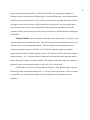
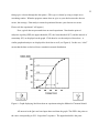
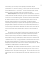
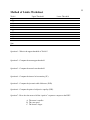
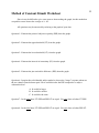
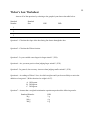
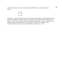
1
Precision and Accuracy
with
Classical Psychophysical Methods
A work in progress by (alphabetical order):
Alistair P. Mapp
York University, Toronto, Ontario, Canada
Hiroshi Ono
York University, Toronto, Ontario, Canada
Josée Rivest
York University, Toronto, Ontario, Canada
Kenzo Sakurai
Tohoku Gakuin University, Sendai, Japan
User’s Manual
2
Contents
Introduction................................................................................................ 3
Organization of the Package...................................................................... 4
Menu ................................................................................................. 4
Introduction............................................................................ 5
Measuring Precision & Accuracy.......................................... 5
Applying Precision & Accuracy ............................................ 5
Review Quiz............................................................................ 6
Sample Experiments .............................................................. 6
Sub-menus ....................................................................................... 6
Overview and Objectives ....................................................... 7
Operating Instructions........................................................... 7
Tutorial and Quiz................................................................... 7
Experiment and Data Analysis ............................................ 14
Psychophysical Dictionary ....................................................................... 19
Postscript .................................................................................................. 22
References................................................................................................. 29
Acknowledgements................................................................................... 31
Worksheets ............................................................................................... 32
Method of Limits .................................................................. 33
Method of Constant Stimuli................................................. 35
Method of Adjustment ......................................................... 37
Weber’s Law......................................................................... 39
Mueller-Lyer Illusion ........................................................... 41
Expt. l: JND and PSE with two
psychophysical methods....................................................... 43
Expt. 2: Mueller-Lyer Illusion
with different lengths of lines .............................................. 45
Expt. 3: Measuring the Ponzo Illusion ................................ 47
Introduction
This package introduces the psychophysical concepts of precision and accuracy. First
you will learn how to measure precision and accuracy with the method of limits, the method of
constant stimuli, and the method of adjustment. Then you will learn how to describe
experimental results in terms of precision and accuracy. In doing all of this, you will examine
how long one line must be to appear different or equal in length to another line. The smallest
difference that is reliably discriminated is called the just noticeable difference (JND) and the
average length that appears equal is called the point of subjective equality (PSE). Precision is
said to be high when the JND is small. Accuracy is said to be high when the PSE is close to the
actual value.
The two concepts, precision and accuracy, are closely related to concepts you encounter
in other psychology courses. Precision is related to the concept of variability (standard
deviation, quartile deviation, or range) discussed in a statistics course, and to the concept of
reliability or random error (“noise”) discussed in a course in measurement. Accuracy is closely
related to a central tendency (mean, median, or mode) discussed in a statistics course, and to the
concept of validity or “bias” discussed in a course in measurement.
As you go through this package, you will learn how to use the three psychophysical
methods presented and also learn the differences between precision and accuracy. This learning
process can be both easy and enjoyable. All you need to do is follow the instructions that appear
on your computer screen. When a question is asked or when a menu appears, respond to it by
moving the “mouse,” which moves the “pointer” on the screen. When several “buttons”
(options) are presented, use the mouse to move the pointer to the desired button and then “click.”
3
Organization of the Package
The manual is organized to reflect the design of the computer program it accompanies.
You will be presented with eight buttons (menu) on the screen; five of them will in turn present
four buttons (sub-menu). The heading of each section of the manual corresponds to the button
presented. If you are uncertain which button you should click, simply look under the
corresponding heading in this manual for further information.
Menu
In the menu, you may choose whichever button you wish in any order you wish. Your
first time through, however, go through the program in the order presented, since later parts
assume that you understand earlier parts.
Figure 2. Menu.
A summary of the function of each button is given below. More detailed information on
some of the buttons is included in later sections. Note that you will need a pencil and paper to
4
5
complete the tutorials. A calculator is provided in the program, but you may wish to use your
own.
Introduction
If this is your first time using the program, click this button and read the text presented.
This is where many important concepts are first introduced and defined. In addition, a
psychophysical dictionary is at your disposal that will further assist you in the understanding of
certain psychophysical concepts. This section gives you a general idea of how the many
concepts introduced in this package are interrelated and also outlines what you are expected to
learn from this package. In subsequent parts of the program, we assume that you understand this
material.
Measuring Precision and Accuracy
There are three buttons under this heading, namely, Method of Limits, Method of
Constant Stimuli and Method of Adjustment. If you click any of these buttons, a sub-menu on
the lower right side of the screen will appear. Figure 3 shows the sub-menu when the “Method
of Limits” is clicked. By clicking the sub-menu buttons, you gain experience with using one of
the psychophysical methods and learn to measure precision and accuracy. By going through the
three sub-menus for the different methods, you will learn how to measure precision and accuracy
with three different methods.
Applying Precision & Accuracy
There are two buttons under this heading, namely, Weber’s Law and Mueller-Lyer
Illusion. When you click either button, the sub-menu that appears is the same as that when you
click one of the buttons for the different methods. By clicking the buttons under Weber’s Law,
you will learn how the law describes precision for different lengths of lines and gain further
understanding of precision. By clicking the buttons under Mueller-Lyer Illusion, you will learn
how the illusion affects accuracy and gain further understanding of accuracy.
6
Review Quiz
This button leads to the quiz that tests your understanding of the material presented in
this package. Answer each multiple-choice question by clicking the choice corresponding to the
correct answer. If you choose the wrong answer, you will be asked to make another choice. If
you do not respond correctly after two attempts, the correct answer will appear on the screen, and
you will proceed to the next question. When you have finished the quiz, a summary of how well
you did will be displayed.
Sample Experiments
This part of the package provides hands-on experience in collecting data and drawing
conclusions. The three experiments are examples of experiments that can be done with this
package. Hopefully, these sample experiments will trigger ideas for generating your own
experiments.
Sub-menus
Below, the general function of each button in the sub-menu is first described, and then
later its specific function when a particular button on the Main Menu has been clicked is
described.
Figure 3. Menu with sub-menu for the Method of Limits now appears.
7
Overview and Objectives
Clicking this button gives you background information and a list of learning objectives
for a particular section.
Operating Instructions
Clicking this button leads to the explanation of how to use the program for the five
topics. For generating your own data in the “Tutorial and Quiz” and “Experiment and Data
Analysis” you must understand the instructions described here. (In the “Method of Adjustment,”
“Weber’s Law,” and the “Mueller-Lyer Illusion,” the type of judgments you are making is the
same and you can either click the buttons or use the arrow keys on the lower parts on the
keyboard for your responses. Try both procedures in the practice trials to see which you are
most comfortable using.) After you have read the instructions, click the “Practice Trials” button
for practice trials. Since no data are collected during these practice trials, experiment with your
responses. In these practice trials and in the tutorial, don’t think too much about the judgment
you are making; your first impression is fine. In all five topics, what you “see” is being
measured, not what you “think.”
Tutorial and Quiz
After you understand the “Operating Instructions,” you continue to “Tutorial and Quiz”
which leads you through an experiment, data analysis and a quiz. The program is designed for
you to generate your own data in working through the tutorials, as this hands-on experience is an
important part of the learning process. However, you can also use previously generated sample
data, if you are pressed for time.
The tutorials require you to estimate or calculate values in screen units from graphs and
tables. The term “screen units” is used because the actual length of a line is determined by the
size of your monitor. Worksheets required for the tutorials are located at the end of this manual.
8
Figure 4. Opening screen of the Tutorial and Quiz for the Method of Limits.
Once you have generated your data (or sample data), an explanation of the analysis will
appear. Make sure that you read and understand what is said here since you will need to perform
the analysis later. Then, questions designed to help you analyze your data are presented and you
can check your answers with the computer’s answers. The answers provided by the computer
are based on rounding to the first decimal place except for calculating the slope in Weber’s Law,
which rounds to the second decimal place. If you use a different rounding procedure or use a
calculator to do the detailed calculations, the answers may be slightly different. If a question
requires a numerical answer, use the keyboard to type in the appropriate numbers. You can also
enter the answer directly from the calculator by clicking the "record" button.
If you have a question about a calculation, you can use the “Calculation Help Menu” to
find the information you need. The Help menu provides explanations and equations and can
assist you in answering questions in the tutorial. If you have forgotten how to perform the
calculations required, just click the “Calculation Help” button. The menu will display a list of
9
topics related to the question asked. Click the desired topic; the appropriate definition or
formula to answer your question will then appear. From the Help menu, you can then return to
the Quiz and answer the question. If you cannot answer after two attempts, the correct answer
will appear on the screen, and you will proceed to the next question. It is also a good idea to
copy down the correct answer for each question on the appropriate worksheet because the
computer will not store your answers and you may need to use a specific number in subsequent
calculations.
Method of Limits. After reading the explanation of the data analysis, you will see your
data (or sample data) presented in a chart. You need not copy down this information since you
will have access to it throughout the tutorial. The chart displays your judgments for each
comparison stimulus length in each trial. An “S” indicates that the comparison stimulus
appeared shorter than the standard stimulus, and an “L” indicates that the comparison stimulus
appeared longer. An “=” indicates that the comparison and standard stimuli appeared equal in
length. The point of objective equality (POE) is the length at which the comparison stimulus is
physically equal to the standard stimulus; in this case it is 50 screen units.
Click ahead to see a chart of typical data (see Figure 5). Note that the response for the
POE length of the comparison stimulus was “=” on every trial except for one. If this is not true
for your data, you were probably making an error of habituation or expectation in your
responses.
10
Figure 5. Chart displaying typical data generated from the Method of Limits.
The Quiz for this method requires some calculation. For each trial, the lower threshold is
halfway between the smallest “=” and the first “S” response, and the upper threshold is halfway
between the largest “=” and the first “L” response. The mean lower threshold is the mean of the
lower thresholds from different trials; the mean upper threshold is the mean of the upper
thresholds from different trials. The mean PSE is midway between the mean lower and mean
upper thresholds or the sum of the two divided by two [(UT+LT)/2]. The JND is one half the
interval between the mean lower and mean upper thresholds or [(UT-LT)/2].
Method of Constant Stimuli. After reading the explanation of the data analysis, you
will see your data presented in a table. You need not copy down these data since you will have
access to this information in graphic form throughout the tutorial. The data table displays the
number of “longer than” responses made for comparison stimuli of various sizes. You will also
see the percentage of “longer than” responses plotted as a function of comparison size. The best
11
fitting ogive is drawn through the data points. (This ogive is drawn by using a simple curvesmoothing routine. When the program cannot draw an ogive to your data because the data are
erratic, the message, “Data analysis cannot be performed because your data are too erratic.
Please redo the experiment” will appear )
Next, typical data are presented from an actual experiment. Note that the point of
subjective equality (PSE), the upper threshold (UT), the lower threshold (LT), and the interval of
uncertainty (IU) are displayed on the graph. Click ahead to see the analysis of these data. A
similar graph and analysis are displayed for ideal data as well (see Figure 6). In this case, “ideal”
means that the data are derived from a cumulative normal distribution.
Figure 6. Graph displaying ideal data from an experiment using the Method of Constant Stimuli.
All answers in the Quiz are based upon data read from the graph. The PSE is the point on
the curve corresponding to 50% “longer than” responses. The upper threshold is the point
12
corresponding to 75% “longer than” responses while the lower threshold is the point
corresponding to 25% “longer than” responses. The JND is one half of the interval between the
lower and upper thresholds, i.e., one half the IU. You may find it helpful to apply a drafting
triangle or a corner of a sheet of paper on the screen to estimate these values.
Method of Adjustment. After reading the explanation of the data analysis, you will see
your data presented in a table and an histogram. You need not copy down this information since
you will have access to it throughout the tutorial. The data table displays the adjusted length of
the comparison stimulus for each trial. The histogram represents the number of times you
adjusted the comparison stimulus to each of several lengths. Note that the histogram is
constructed by dividing the range of comparison values into approximately equal intervals and
plotting the number of adjustments for each interval. If you continue through the analysis you
will see an histogram of ideal data that is bell-shaped. These data are “ideal” because they were
derived from a bell-shaped normal distribution that is expected if you had a large number of
trials.
All calculations in the quiz should be based upon the raw data presented in the table, not
upon data read directly from the histogram, because the data on the histogram represent the
number of responses in each two unit-wide bin. The PSE is the mean of the distribution of
adjusted lengths, and the JND is proportional to the standard deviation of this distribution (JND
= standard deviation x 0.6745). In a normal distribution, the range between the mean score plus
the standard deviation multiplied by 0.6745 and the mean score minus the standard deviation
multiplied by 0.6745 contains 50% of the scores and is sometimes called probably error. The UT
is one JND above the PSE, and the LT is one JND below the PSE.
Weber's Law. After reading the explanation of the data analysis, you will see your data
presented in a table. You need not copy down this information since you will have access to it
throughout the tutorial. Note the three columns in the table. The first column lists the size of the
standard stimulus, the second column reports the PSE, and the third column shows the size of the
JND.
13
Following this table, the program will display three graphs. Click ahead to see a graph of
the size of the JND as a function of the standard stimulus size for your data. The data points
represent the actual data values while the line is the best fitting straight line through the data.
You should note how well the straight line fits your data. Click ahead again to see what a graph
of the data looks like in an actual experiment. Notice that the straight line fits the data fairly well
and that if the size of the standard were close to zero the straight line would predict that the JND
would be close to zero. Click ahead to see a third graph of what the data should look like if
Weber's Law fits the data perfectly. Note that all data lie along a straight line and that if the
standard stimulus was zero, the JND would also be zero (see Figure 7).
Figure 7. Graph displaying Weber’s Law from an experiment producing ideal data.
Mueller-Lyer Illusion. After reading the explanation of the data analysis, click ahead to
see the ideal data presented in a table. Note the four columns in the data table. The first column
displays a picture of each type of standard stimulus. The second and third columns show the
JND and PSE for each standard. The final column reports the constant error calculated from
14
each standard stimulus based upon the POE of 50 screen units. Notice that the constant error for
the illusion is typically about 10% of the POE. The standard stimulus without flanking arrows
should have a small constant error. (Here it is zero).
Experiment and Data Analysis
Clicking this button allows you to design experiments for whichever topic you have
chosen from the Menu. The data analysis part of the program analyzes the data collected from
an experiment that you will design and perform. Unlike the tutorial, there are no quiz items to
answer. Data are displayed in both tables and graphs, and an explanation of the analysis, as
given in the tutorial, is available.
Figure 8. Opening screen of the Experiment and Data Analysis option for the Method of Limits.
Below are comments on the different variables that can be manipulated in the
“Experiment and Data Analysis.”
15
Measuring Precision & Accuracy. For each of the methods, the opening screen shown
in Figure 8, or a similar one, will appear and you can design an experiment to determine the
effects of changing one of the following experimental variables.
Standard stimulus: The length of the standard stimulus was set for 50 screen units in the tutorial.
You can vary the standard between 15 and 190 screen units.
Comparison stimuli: For the methods of limits and constant stimuli, you can vary the range of
the comparison stimulus values and the value of the midpoint of the range. The available ranges
are 5, 10, 15, 20 and 40 screen units; the available midpoints are 7 to 210 screen units. In the
tutorial the range was 10 units and the midpoint was 50 units. Since there are 21 equally spaced
comparison stimuli in the method of limits and 11 in the method of constant stimuli , the range of
10 units provided a 0.5-unit difference between the two “nearest” comparison stimuli for the
method of limits and a 1-unit difference for the method of constant stimuli. If you choose a
different range, the unit difference will automatically change proportionately; e.g., the range of
20 units would produce a difference of 1 unit for the method of limits and a difference of 2 units
for the method of constant stimuli. The range you choose must be larger than the IU and the
difference between the two “nearest” comparison stimuli must be smaller than the JND. You
will need a small range for a small standard stimulus and a larger one for a larger standard
stimulus. (The reason for this requirement should become apparent when you study Weber’s
law.) The midpoint will automatically change with the change in standard stimulus (POE), but
you may want to have the midpoint of a range different from the POE when you think that the
PSE will differ from the POE. In the method of adjustment, the range is set automatically to
20% of the standard stimulus and the midpoint is set to the POE. For example, if the standard
stimulus is 100 units, the range is set for 90 to 110 units.
Top line: You can set the top line to be either the standard stimulus or the comparison stimulus.
It is the standard stimulus in the tutorial.
Horizontal separation: While the standard stimulus and the comparison stimulus in the tutorials
come onto the screen at random locations (vis-à-vis their horizontal separation from each other),
16
you can choose to present the lines in fixed horizontal locations in your experiment. The
standard and comparison stimuli are set to appear at random screen locations, but if you want
them to appear in fixed locations, click the “fixed” button. Then, choose the desired separation
of the fixed locations. Possible separations vary between 0 and 195 screen units, depending on
the standard stimulus length. A separation of 0 means that the standard will be directly over or
under the comparison.
Vertical separation: You can change the vertical separation between the standard and the
comparison to be between 10 and 170 screen units.
Number of trials: You can vary the number of trials between 10 and 100 for the method of
limits, between 40 and 150 for the method of constant stimuli, and between 10 and 40 for the
method of adjustment.
Presentation order or Starting position: You can choose to have descending trials only,
ascending trials only, or counterbalanced between ascending and descending trials. This option
is not available in the method of constant stimuli.
Applying Precision and Accuracy. The experiments with Weber’s Law and the
Mueller-Lyer illusion in this package use the method of adjustment. Hence, the opening screen
that appears is like that of the method of adjustment and the computer chooses the range and the
midpoint of the comparison stimuli. As you can see in Figure 9, you can manipulate the
variables you did in the method of adjustment: top line, horizontal separation, number of trials
and starting position. Unlike the experiments with the method of adjustment, you can vary the
number of stimuli between 2 and 7. For the Mueller-Lyer illusion experiment, a menu very
much like that for the method of adjustment will appear but the horizontal separation may be
varied between 0 and 195 screen units and the vertical separation can be varied between 20 and
170.
17
Figure 9. Opening screen of the “Experiment and Data Analysis” for Weber’s Law.
Possible Experiments. Below are some experiments you might try. You should try to
create your own experiments as well, since the creative act of designing an experiment can be as
valuable as actually executing the design.
By choosing different values for the variables you can learn more about the topics. You
can vary the number of trials in different sections to learn about the stability of an obtained JND,
PSE, Weber fraction, or the extent of the Mueller-Lyer illusion as a function of the number of
trials. Also, you can use a small range of comparison stimulus values with a large standard
stimulus in the methods of limits and constant stimuli, and learn about these methods. You will
find that the JND cannot be measured when the set of comparison stimuli is not appropriate for
the standard stimuli. Such an experience would give you an idea of what you must take into
consideration in choosing the comparison stimuli when you want to use these methods to
18
measure the JND and the PSE for stimuli other than the lengths of lines, such as the amount of
light or weight.
Besides learning more about each topic, you can gain experience in designing your own
experiments. An experiment might involve systematically varying the horizontal or vertical
separation of the standard stimulus and comparison stimulus to discover changes in the JND,
Weber fraction, or the extent of the Mueller-Lyer illusion. Eliminating the random horizontal
placement of the comparison stimulus or placing the standard stimulus and comparison stimulus
closer together should allow subjects to develop more effective judgment strategies, which in
turn, should reduce the size of the JND or the extent of the illusion. Weber’s law is said to fail
under this condition (Weber, 1849) and you can design an experiment to find this out for
yourself.
Experiments need not be limited to manipulating the variables in the menu. You can
compare the three psychophysical methods with each other. (See Experiment I in the Sample
Experiments section and discussion of Figure 11 in this manual.) You may want to examine the
effect of different lengths of lines on the Mueller-Lyer illusion. (See Experiment II in the
Sample Experiments section of this manual.)
The “Experiment and Data Analysis” can be used in conjunction with some external
manipulation. You might hypothesize that subjects with glasses (or contact lenses) would
produce smaller JNDs than the same subjects not wearing glasses (or contact lenses). Subjects
could be asked to run the experiment twice, once with their glasses (or contact lenses) and once
without. Don’t forget to counterbalance the order of testing across subjects. You can also
measure the extent of the Ponzo illusion by attaching masking tape on the computer screen. (See
Experiment III in the Sample Experiments section.) How about measuring the verticalhorizontal illusion by attaching a sheet of paper with vertical and horizontal lines for a standard
stimulus? For more example experiments, see the worksheets on pages xx, yy, and zz of this
manual.
Psychophysical Dictionary
The following eighteen terms are defined in the dictionary:
1. Comparison (Variable) Stimuli: a set of stimuli judged relative to a standard stimulus. In the
method of limits, a series of comparison stimuli is presented in ascending (“less than” to “more
than”) or descending (“more than” to “less than”) order, and a subject judges the comparison
stimulus as “more than,” “equal to, ” or “less than” the standard stimulus for each trial. In the
method of constant stimuli, one of the comparison stimuli is randomly chosen for a trial, and a
subject judges the comparison stimulus as “more than” or “less than” the standard stimulus. In
the method of adjustment, a subject adjusts the comparison stimulus to appear equal to the
standard stimulus.
2. Constant Error: a systematic error in judgment in which the point of subjective equality (PSE)
is significantly larger or smaller than the point of objective equality (POE). For example, if you
consistently guess the height of a 9 meter high pole to be 10 meters, you would be making a
constant error of one meter. Constant error is defined as the point of subjective equality (PSE)
minus the point of objective equality (POE). A positive value indicates the mean judgment to be
larger than the real value and a negative value indicates the mean judgment to be smaller. The
absolute value of the constant error is inversely related to accuracy.
3. Counterbalancing: a technique for “removing” from the experimental results the effect of the
order of presentation. For example, if you asked a group of people to compare the tastes of Coke
and Pepsi, your experiment would be counterbalanced, if half of your subjects tasted Coke before
Pepsi and half tasted Pepsi before Coke.
4. Error of Expectation (Anticipation): the tendency to make a response before it is appropriate
to do so. If in the method of limits a subject anticipates the equal stimulus and responds “equal
to” prematurely, he/she would be making an error of expectation. For example, if a runner
started racing before the gun went off, he/she would be making an error of expectation.
5. Error of Habituation: the tendency to continue making the same response after that response
is no longer appropriate. For example, if in the method of limits a subject becomes accustomed
to making a “more than” judgment and continues making this response longer than necessary,
he/she would be making an error of habituation. Trying to stroke your beard when you shaved it
off yesterday, or going to last year’s locker the first day of classes are other examples of errors of
habituation.
6. Interval of Uncertainty (IU): the range of values of the comparison stimulus in which the
comparison stimulus cannot be reliably discriminated from the standard stimulus. The range is
two JNDs, and it spans from one JND below the PSE to one JND above the PSE. For example, a
10.001 cm-long comparison line would be within the interval of uncertainty for a standard
stimulus 10.000 cm long. As well, a comparison piece of cherry pie weighing 0.333 kg would
probably be within your interval of uncertainty for weight discrimination if the standard was a
piece of pie weighing 0.334 kg.
19
20
7. Just Noticeable Difference (JND): the smallest difference between stimuli that can be reliably
discriminated 50% of the time. The just noticeable difference (JND) is also known as the
difference threshold (DT) and the difference limen (DL). For example, if a line length of 10.3
cm is reliably judged longer when compared with a line length of 10 cm, the JND is 0.3 cm. In
the method of limits and the method of constant stimuli, the JND is one half of the interval of
uncertainty (IU). In the method of adjustment, the JND is 0.6745 multiplied by the standard
deviation of the responses. If a set of lights of various brightnesses were compared to a standard
light, it would be very easy to tell that some lights were brighter or dimmer than the standard
(more than one JND from the standard). Other lights from the set, however, would be difficult to
distinguish from the standard (less than one JND from the standard).
8. Lower Threshold (LT): the largest comparison stimulus reliably judged to be less than the
standard. In the method of limits, the lower threshold in a descending trial is defined as the
stimulus value halfway between the value of the last “equal to” response and the value of the
“less than” response; in an ascending trial, it is the stimulus value halfway between the last “less
than” response and the first “equal to” response. In the method of constant stimuli, the lower
threshold is the stimulus value that evokes the “more than” response 25% of the time, or the “less
than” response 75% of the time. In the method of adjustment, it is the mean of the subjects’
adjustments minus 0.6745 multiplied by the standard deviation (PSE-JND). For example, the
largest ice cream cone which you can tell is smaller reliably than a standard cone is a lower
threshold.
9. Normal Distribution: a distribution of scores whose graphic representation has a bell-shaped
form. For example, heights tend to be normally distributed. Very few adults are either
extremely tall (more than 2.1 meters or 7 feet) or extremely short (less than 1.2 meters or 4 feet),
while most adults are close to the average height (1.7 meters or 5 feet 8 inches for males - 1.6
meters or 5 feet 3 inches for females).
10. Ogive: an S-shaped curve in appearance; also called a “Sigmoid” curve. The curve takes
this shape when one plots the percentage or frequency of scores in a normal distribution that are
less than or equal to given values. For example, since heights follow a normal distribution, if we
were to plot the percentage of people whose heights are less than or equal to different values, this
curve would be shaped like an ogive.
11. Point of Objective Equality (POE): the point at which the comparison stimulus value
physically equals the value of the standard stimulus. For example, if the strength of a set of
perfumes were compared to a standard perfume whose strength was 7, then the POE would be 7.
12. Point of Subjective Equality (PSE): the point at which a comparison stimulus is judged equal
to the standard stimulus. In the method of limits, it is both the midpoint between the UT and LT
and the mean of the stimulus values that evoke “equal to” responses. In the method of constant
stimuli, it is the stimulus value that evokes the “more than” or “less than” response 50% of the
time. In the method of adjustment, it is the mean value of the adjustments. For example, if we
wanted to determine the perceived size of the moon, we might have subjects adjust a disk to
equal the perceived size of the moon. If the average adjusted size of the disk is 10 cm. squared,
then the PSE is 10 cm. squared.
13. Precision and Accuracy: two independent qualities of a set of judgments. Precision is said to
be high when the variability of the judgements (JND) is small. Accuracy is said to be high when
the central tendency of the judgements (PSE) is close to the actual value. For example, a set of
darts scattered evenly around the bull's-eye of a dartboard demonstrates low precision;
nonetheless, the accuracy is high, since the average dart position is the bull's-eye. (See Figure 10
in this manual.)
14. Response Bias: a procedural or nonsensory factor that influences responses to stimuli. The
errors of expectation and habituation are response biases that can be identified when using the
method of limits.
15. Standard Stimulus: the stimulus for which you wish to determine a psychophysical value,
and to which comparison stimuli are judged or adjusted. If you wish to determine the JND for a
10 cm line length, the 10 cm line that you use to do this is the standard stimulus.
16. Upper Threshold (UT): the smallest comparison stimulus reliably judged to be greater than
the standard. In the method of limits, the upper threshold in a descending trial is defined as the
stimulus value that is halfway between the last “more than” response and the first “equal to”
response; in an ascending trial, it is the stimulus value halfway between the last “equal to”
response and the “more than” response. In the method of constant stimuli, the upper threshold is
the stimulus value that evokes the “more than” response 75% of the time, or the “less than”
response 25% of the time. In the method of adjustment, it is the mean of the subject's
adjustments plus 0.6745 multiplied by the standard deviation (PSE + JND). As an example, the
smallest slice of bread you can still tell is larger reliably than a standard slice is an upper
threshold.
17. Variable Error: unsystematic error in judgments. The higher the JND, the larger the variable
error. A large variable error shows low precision; a small variable error shows high precision.
18. Weber's Law: a statement that the magnitude of the JND is a constant proportion of the
standard stimulus intensity. For example, a large person must lose more weight than a small
person before other people will notice that they lost weight. Mathematically, Weber’s Law is
expressed:
JND = K x S
where JND is the size of the just noticeable difference, K is a constant known as the Weber
fraction, and S is the size of the standard stimulus. Modern psychophysics has modified this
equation to take into account that perception starts at a non-zero value. The modified equation is
JND = K x S + C, where C is a constant.
21
Postscript
Although in casual speech the two words “precision” and “accuracy” are used
interchangeably, you must resist the temptation to do so in the context of psychophysical
measurement. I hope you no longer have this temptation after going through this package. Once
you grasp the distinction, it is difficult to figure out why this distinction gives students difficulty.
Perhaps, the difficulty is related to the concepts of precision and accuracy being statistical
abstractions. That is, one cannot make a statement about precision for a single judgment.
Precision and accuracy are abstractions or summaries of a set of judgments just as mean and
standard deviation are abstractions or summaries of a set of scores. To recapitulate, precision is
the opposite of variable error; accuracy is the opposite of constant error. They refer to two
independent aspects of a set of judgments. That is, knowing how precise subjects are in judging
the length of a line tells you nothing about how accurate they are; knowing how accurate they are
tells you nothing about how precise they are. To state the same in terms of the psychophysical
variables defined in the beginning of this package, knowing the size of the JND tells you nothing
about the distance between the POE and the PSE and vice versa. Precision and accuracy as
independent concepts are illustrated in Figure 10.
22
23
Figure 10. Illustration of precision and accuracy as independent concepts. Each column (A, C
and B, D) has the same precision and each row (A, B and C, D) has the same accuracy. In (A),
accuracy may not appear high because the “center” of the dart loci appears to be in the right-top
quadrant. This is an optical illusion due to the “slant” of the darts; the point defined by the
average horizontal location and that of the vertical location falls on the bull’s-eye.
Since precision and accuracy are independent, response bias or experimental procedure
can affect one without affecting the other. For example, in the method of limits, a response bias
of saying “equal to” would increase the size of the JND, and a bias of not saying "equal to"
would decrease the JND’s size. These biases would affect the precision but not the accuracy.
24
For another example, in the method of adjustment, if only descending trials are used, an error of
expectation would produce responses greater than the point of objective equality (POE). This
procedure would decrease accuracy (would produce a positive constant error) without affecting
precision. One can remove this constant error by counterbalancing the trials, i.e., presenting the
same number of ascending and descending trials. Shifts in the point of subjective equality (PSE)
on descending trials would be offset by shifts in the opposite direction on ascending trials.
However, this removal of the constant error decreases precision. That is, with this procedure, an
error of expectation produces adjustments greater than the PSE on descending trials and less than
the PSE on ascending trials.
Experimental procedures in the psychophysical method you choose should reflect
whether the focus of the experiment is on precision or accuracy. For example, precision was the
main interest in the examination of Weber’s Law; thus the concern should be with eliminating
any bias from the measurement of the JND. For this reason, counterbalancing the ascending and
descending trials in the method of adjustment would produce a larger variable error, if an error of
expectation or habituation was operating. If such an error is large, the method of constant
stimuli, which is free of the effect of this error, can be used. In contrast, accuracy, or lack of it,
was the main interest in measuring the extent of the Mueller-Lyer Illusion. The aim was to
measure the constant error due to “arrow direction,” free of any constant error resulting from
procedural or response bias. In this case, counterbalancing would remove the bias in the PSE
due to an error of either expectation or habituation. (A purist would also counterbalance the topbottom location of the standard stimulus to control for the tendency of a stimulus in the upper
visual field to appear as large as one in the lower visual field.) To summarize, it is important for
an experimenter to (a) be clear about what is being measured, precision or accuracy, and (b)
eliminate the possible sources of bias that can contaminate what is being measured.
Theoretically, all three methods should yield the same values for point of subjective
equality (PSE), just noticeable difference (JND), interval of uncertainty (IU), and upper and
lower thresholds (UT and LT), although the values for these variables were derived in a different
25
order in each method. (See Figure 11.) In the method of limits, the UT and LT were determined
first and then the IU, PSE, and JND were derived. In the method of constant stimuli, the UT,
PSE, and LT were determined first and then the IU and JND were derived. In the method of
adjustment, the PSE and JND were calculated first and then the IU, UT, and LT were derived. In
practice, however, the values from the different methods are seldom the same, as you probably
found out in doing the Sample Experiment 1. The different values come about because each
method is subject to different sources of bias and error. (To find out more about response bias,
or factors that affect our judgment, look into adaptation level theory and signal detection theory
cited in the reference section.)
26
Figure 11. Illustration of theoretically equal values of psychophysical variables obtained with
three methods. The meaning of the ideal data is different for different panels. The data on the
top panel are ideal in that responses to given stimulus values were always the same. If this were
true for the lower two panels, the two functions would have steps. The function on the second
panel is ideal in that the data is derived from the bell-shaped (normal) curve and that on the third
panel is ideal in that it is a bell-shaped curve. The tail ends of the curves in the second and third
panels are truncated to enlarge the relevant portions of the function.
27
Which method is the best? Each method has advantages and disadvantages, and hence no
single method is the best under all circumstances. The method of limits can be the least timeconsuming. The method of constant stimuli is the least sensitive to response biases, but it
requires many more trials. In addition, choosing the appropriate comparison stimuli to use with
this method requires a pilot experiment. The method of adjustment has the advantage that the
experimenter does not have to choose the comparison stimuli. Which method is best depends on
such factors as what psychophysical variable you are concerned with and time constraints.
This package, as an introduction to psychophysical methods, is incomplete in that it does
not discuss how to measure absolute threshold nor the newer methods. The three methods
discussed in this package can also be used to measure absolute threshold, i.e., a stimulus value
that can be detected 50% of the time. How to measure absolute threshold was not illustrated in
this package because the stimulus value near the absolute threshold is difficult to control without
additional equipment. By going through this package, however, it is easier to understand how to
measure absolute threshold. The latest methods of measuring thresholds are variations of the
method of limits and are known as the “staircase” and “PEST” (Parameter Estimation by
Sequential Testing) procedures. These methods were not considered here because they exceed
the scope of this package, but understanding the method of limits covered in this package will be
helpful in understanding these methods. (For further information, refer to one of the books listed
in the “References” section of this manual.)
The topic of psychophysics has a long history and is relevant to other topics in
psychology. The three methods in this package are those used by Fechner (1860/1966), who
founded the science of psychophysics. Weber’s law, which you learned about in this package,
served as a building block of what is known as Fechner’s law which attempts to state the relation
between the magnitude of a physical stimulus and the psychological experience caused by it.
Every area in psychology requires the measurement of variables, be it “anxiety” in clinical
psychology, “attitude” in social psychology, or “JND” in experimental psychology. Whatever
28
you want to measure, you should note how precise and accurate an obtained score is.
Sometimes the extent of inaccuracy itself is of interest, as in the Mueller-Lyer illusion you
measured. In this case, the goal is to measure the inaccuracy caused by the direction of arrows
and not by other factors such as the order of presentation. To do this, a counterbalancing
technique was used. Whatever area of psychology you pursue, the use of such a technique to
remove the undesirable inaccuracy is expected. I also hope this package serves as a first step in
going on to study the area of psychophysics. My hope is that what you have learned through this
package will serve you well in all areas of psychology and related disciplines.
References
Most perception textbooks provide a description of the concepts and the methods
discussed in this package. The following are a few recommended sources:
Introductory Readings
Coren, S. & Ward, L.M. (1989). Sensation & perception (3rd Ed.). U.S.A.: Harcourt Brace
Jovanovich.
Galanter, E. (1962). “Contemporary psychophysics.” In (T. Newcomb, ed.) New directions in
psychology. New York: Holt, Rinehart and Winston.
Goldstein, E.B. (1989). Sensation and perception. (3rd Ed.). Belmont, CA: Wadsworth.
Schiffman, H.R. (1990). Sensation and perception: An integrated approach (3rd Ed.). U.S.A.:
John Wiley & Sons.
Sekuler, R. & Blake, R. (1990). Perception (2nd Ed.). U.S.A.: McGraw-Hill.
More Advanced Readings
Baird, J.C., & Noma, E. (1978). Fundamentals of scaling and psychophysics. New York: John
Wiley & Sons.
Falmagne, J.C. (1986). Psychophysical Measurement and Theory. In K.R. Boff, L. Kaufman,
& J.P. Thomas (Eds.), Handbook of perception and human performance: Volume 1.
Sensory processes and perception (pp. 1-66). U.S.A.: John Wiley & Sons.
Fechner, G. T. (1860/1966). Elements of Psychophysics, Vol. 1. Translated by H. E. Adler.
New York: Holt, Rinehart and Winston.
Kling, J.W., & Riggs, L.A. (1971). Experimental psychology (3rd Ed.). New York: Holt,
Rinehart and Winston.
Underwood, B.J. (1979). Experimental psychology. New York: Appleton-Century-Crofts.
Weber, E. H. (1849). “Der Tastsinn und das Gemeingefuel.” In (R. Wagner, ed.)
Handworterbuch der Physiologie, III. Braunschweig: Bieweg.
29
Readings on Specific Questions
For a brief discussion of response bias and presentation order, see the Postscript in this
manual.
In the Weber’s Law tutorial, the study which supplies the data for the “Typical Data”
graph is:
Ono, H. (1967). “Difference threshold for stimulus length under simultaneous and
nonsimultaneous viewing conditions.” Perception and psychophysics, 2, 201-207.
The reason for the y-intercept being greater than zero in the graph is discussed in:
Galanter, E. (1962). “Contemporary psychophysics.” In (T. Newcomb, ed.) New directions in
psychology. New York: Holt, Rinehart and Winston.
and
Miller, G.A. (1947). “Sensitivity to changes in the intensity of white noise and its relation to
masking and loudness.” J. Acoust. Soc. Amer., 19, 609-619.
30
Acknowledgements
This package is based on two other packages, namely, Classical Psychophysical Methods
and Accuracy and Precision, which are distributed by Conduit. Some parts of this package are
the same as parts of the two original packages, and the contributions of Mark Wagner and
Kenneth Ono, the co-authors of the two original packages, are acknowledged for this package.
They were able to spend only limited time on this package because of their other commitments.
Their participation was greatly missed. There are a number of people who spent a considerable
amount of time on this package. Gayle Brock oversaw the whole project to its completion
through two summers. Mark Stock took over the programming chore, from Joe Porrovecchio
who started the programming with Kenzo Sakurai, and is primarily responsible for the final
software. Among the many people who worked through the packages and suggested
improvements, Raynald Comtois, Carol Dengis, Herb Goltz, Lorraine Gunther, Al Mapp,
Masaaki Okura, Haruhiko Ohtubo, Krista Phillips, Josee Rivest, Koichi Shibuta and Pete Trotter
were most helpful. The experiments listed in the Sample Experiments section were first
designed for a class taught by Al Mapp and Hiroshi Ono. The preparation of this package was
supported by The Institute for Space and Terrestrial Science (ISTS) and by Grant A0296 from
the Natural Sciences and Engineering Research Council of Canada.
31
Worksheets
Eight sets of worksheets are included in this section of the package. One each for five
tutorials and three for sample experiments. The worksheets for the tutorials provide space to
record data and to record the answers for the questions that will be asked by the computer. The
worksheets for the sample experiments provide space to record the results analyzed by the
computer, and to answer questions related to the experiments. The questions here do not appear
on the computer screen.
The sample experiments in this manual were designed to give you hands-on experience in
collecting data and drawing conclusions from these data. The sample experiments are presented
in a simple step-by-step fashion so that you can follow along with ease. However, if you are
finding the procedure for the sample experiments hard to follow, just ask your instructor for
assistance. In the first experiment, you will compare data collected by the Method of Limits and
the Method of Constant Stimuli. Experiment I (Condition A) and Experiment I (Condition B)
are designed to be completed by two students, but there is no reason why you cannot do it by
yourself. In the second experiment, you will examine the effects of varying the lengths of the
standard stimulus in measuring the Mueller-Lyer Illusion, and in the third experiment you will
examine the Ponzo Illusion using the Method of Adjustment.
It will be helpful if you have a pencil and some scrap paper.
32
33
Method of Limits Worksheet
Trial #
1
2
3
4
5
6
7
8
9
10
Upper Threshold
Lower Threshold
Sum
Mean
Question 1: What is the upper threshold of Trial #1?
Question 2: Compute the mean upper threshold.
Question 3: Compute the mean lower threshold.
Question 4: Compute the interval of uncertainty (IU).
Question 5: Compute the just noticeable difference (JND).
Question 6: Compute the point of subjective equality (PSE).
Question 7: How does the mean of all the “equal to” responses compare to the PSE?
A. The mean is smaller.
B. They are equal.
C. The mean is larger.
Question 8: Is there an error of expectation, habituation, or neither?
A. Expectation.
B. Habituation.
C. Neither.
Question 9: If one subject made only one “equal to” response on each trial and a second subject
averaged seven “equal to” responses on each trial, then which subject would produce the bigger
JND?
A. The first subject.
B. The second subject.
C. Both JNDs would be equal.
Question 10: If there are an equal number of ascending and descending trials, which subject,
from Question 9, would produce the bigger PSE?
A. The first subject (1 “equal to” response per trial).
B. The second subject (7 “equal to” responses per trial).
C. Both PSEs would be equal.
34
Method of Constant Stimuli Worksheet
Since it may be difficult to give exact answers from reading the graph, for this method an
acceptable correct answer has a range of +/- 0.5.
All questions may be answered by referring to the graph of your data.
Question 1: Estimate the point of subjective equality (PSE) from the graph.
Question 2: Estimate the upper threshold (UT) from the graph.
Question 3: Estimate the lower threshold (LT) from the graph.
Question 4: Estimate the interval of uncertainty (IU) from the graph.
Question 5: Estimate the just noticeable difference (JND) from the graph.
Question 6: Imagine that a left-handed subject tended to choose the “longer” response whenever
the two stimuli seemed almost equal. How would this alter the PSE compared to a subject
without this bias?
A. It would be larger.
B. It would be smaller.
C. It would be the same.
Question 7: In the ideal data, UT-PSE and PSE-LT are equal. For your data, calculate UT-PSE.
Question 8: In the ideal data, UT-PSE and PSE-LT are equal. For your data, calculate PSE-LT.
35
Question 9: UT-PSE and PSE-LT are both estimates of the “true” JND. Is the mean (average)
of these two estimates equal to the JND computed in question 5? (Answer Yes or No.)
36
37
Method of Adjustment Worksheet
For this method, your answers should be rounded off to one decimal place. Please be
aware that answers may differ slightly if the rounding procedure is different.
Trial #
1
2
3
4
5
6
7
8
9
10
11
12
13
14
15
16
17
18
19
20
Sum
Mean
Length
(Length - Mean)2
(Length - Mean)
Std. Dev.
Question 1: Compute the mean of your data.
Question 2: Compute the standard deviation.
Question 3: Compute the just noticeable difference (JND).
JND
38
Question 4: Compute the point of subjective equality (PSE).
Question 5: Compute the upper threshold (UT).
Question 6: Compute the lower threshold (LT).
Question 7: Compute the interval of uncertainty (IU).
Question 8: Which one of the following reflects how unreliable or variable your responses
were?
A.
B.
C.
D.
UT and LT.
PSE.
UT or LT.
JND and IU.
Question 9: If 10 units were added to each of your adjustments, which of the values you have
calculated would not change?
A.
B.
C.
D.
E.
PSE.
JND.
UT.
All would change.
None would change.
Question 10: In the method of adjustment, the comparison stimulus starts obviously “longer” or
“shorter” than the standard stimulus. Imagine that all the trials started with the obviously
“longer” stimulus and that the subject had a tendency to leave their finger on the arrow key too
long (i.e., an error of habituation). Which of the following would occur?
A.
B.
C.
D.
JND would increase.
JND would decrease.
PSE would increase.
PSE would decrease.
39
Weber’s Law Worksheet
Answer all of the questions by referring to the graph of your data or the table below.
Standard
Number
Standard
Size
PSE
JND
1
2
3
Question 1: Calculate the slope of the best fitting line drawn through the data.
Question 2: Calculate the Weber fraction.
Question 3: Is your variable error larger for larger stimuli? (Y/N).
Question 4: Are you more precise when judging larger stimuli? (Y/N).
Question 5: In general, does accuracy increase when judging smaller stimuli? (Y/N).
Question 6: According to Weber’s Law, for which weight would you be most likely to notice the
addition of ten grams? (Weber fraction for weight is 0.07).
A. 1 Kilogram.
B. 2 Kilogram.
C. 3 Kilogram.
Question 7: Assume that a weight discrimination experiment produced the following results:
Standard Stimulus
50 g
100 g
200 g
JND
2g
4g
8g
According to Weber’s Law, how large should the JND be for the standard stimulus of
400 g?
A. 10 g.
B. 12 g.
C. 16 g.
Question 8: Consider redoing the tutorial experiment with the Method of Constant Stimuli using
14 different comparison stimuli with the same stimulus value range for the three different line
lengths. Assume that the shortest comparison stimulus produced 20% “longer” responses for the
shortest comparison stimulus and 85% for the longest. If Weber's Law holds, can the
comparison stimuli range be the same for the longer lengths of lines? (Y/N).
40
41
Mueller-Lyer Illusion Worksheet
Answer all of the questions by referring to the table below.
Condition
Number
Standard
1
>--------<
2
I--------I
3
<-------->
JND
PSE
POE
Question 1: Does the direction of the arrows affect the size of the point of subjective equality
(PSE)? (Y/N).
Question 2: Compute the constant error for condition #1.
Question 3: Compute the constant error for condition #2.
Question 4: Compute the constant error for condition #3.
Question 5: For which condition are you most accurate?
Question 6: In which condition are you most precise?
Question 7: An experimenter found a constant error of 5 in a condition A and -5 in a condition
B. In which condition were subjects more accurate?
A. Condition A.
B. Condition B.
C. The conditions are equally accurate.
Question 8: In an experimental procedure using only descending trials, subjects displayed a
positive constant error. What is the probable cause of these results?
A. An illusion.
B. An error of expectation.
C. Both are possible.
42
Name: _____________________________
Student Number: _____________________
Expt. I: JND and PSE with two Psychophysical Methods
Purpose:
The purpose of this experiment is to collect data that will enable you to answer
the following question: Does the Psychophysical Method we use have any effect
on the results we obtain?
Method:
You will answer this question by performing a two condition, counterbalanced
experiment. In Condition A (Method of Constant Stimuli) you will measure the
JND, PSE etc., using the Method of Constant Stimuli, and in Condition B
(Method of Limits) you will measure the JND, PSE etc., using the Method of
Limits.
Procedure:
Step 1. From the Method of Constant Stimuli menu choose the option entitled
Experiment and Data Analysis.
Step 2. Perform the experiment by choosing the button entitled Begin
Experiment and record your data under the column labeled Method of
Constant Stimuli - Run 1 in the table below.
Step 3. Redo steps 1 and 2 above, however, this time use the Method of Limits,
and record your data under the column labeled Method of Limits - Run
1 in the table below.
Step 4. Have a friend perform the same two experiments but have him/her
perform them in the reverse order (i.e., Method of Limits first and
Method of Constant Stimuli second). Record your friend’s data under
the columns labeled Run 2 in the table below.
Step 5. Calculate the mean of Run 1 and Run 2 by adding the obtained values
and dividing the sum by 2. Record these results in the column labeled
Mean in the table below.
Step 6. Answer the questions on the following page.
Experiment Summary
Method of Constant Stimuli
Run 1
POE:
PSE:
JND:
Lower threshold:
Upper threshold:
IU:
Number of trials:
Run 2
Mean
Method of Limits
Run 1
Run 2
Mean
43
Name: _____________________________
Student Number: _____________________
Questions
1. You have learned that when using the Method of Limits subjects often make errors of
habituation and errors of expectation. Another common error associated with the Method of
Limits is that on a given trial subjects tend to make very few equal to responses. Until now
there has not been any name given to this type of error. What do you think this error should
be called? (Note: There is no right or wrong answer, so be creative.)
2. Assuming that the unnamed error discussed in question one did occur, how would you expect
the PSE and the JND as measured using the Method of Constant Stimuli to differ from the
PSE and the JND as measured using the Method of Limits? Why? (Hint: The error is
specific to the Method of Limits and does not occur in the Method of Constant Stimuli.)
3. Do your data show evidence of the error discussed in question one? Explain your answer.
4. What was the purpose of steps 4 and 5? In other words, if you had not performed those steps
what types of alternative explanations could be put forward to explain your results?
44
Name: _____________________________
Student Number: _____________________
Expt. II: Mueller-Lyer Illusion with two different line lengths
Purpose:
The purpose of this experiment is to collect data which will enable you to answer
the following question: What effect does varying the length of the standard
stimulus have on the Mueller-Lyer illusion?
Method:
You will answer this question by performing a two-condition experiment. In
Condition A (Short) you will measure the Mueller-Lyer illusion using a standard
stimulus of 30 units in length, and in Condition B (Long) you will measure the
illusion using a standard stimulus of 140 units in length.
Procedure:
Step 1. From the (In)accuracy and M-L illusion menu choose the option entitled
Experiment and Data Analysis.
Step 2. Set the length of the standard stimulus to 30 units by choosing the
appropriate arrow button.
Step 3. Perform the experiment by choosing the button entitled Begin
Experiment and record your data under the columns labeled Short in the
tables below.
Step 4. Redo the experiment, this time setting the length of the standard
stimulus to 140 units, and record your data under the columns labeled
Long in the tables below.
Step 5. Answer the questions on the following page.
Experiment Summary
JND
Arrow Direction
Short
PSE
Long
Short
Long
>--------<
I---------I
<------>
Short
POE:
Number of trials:
Top line:
Horizontal separation:
Vertical separation:
Presentation order:
Long
Constant Error
Short
Long
45
Name: _____________________________
Student Number: _____________________
Questions
1. According to your data, did the illusion occur for both the Short and the Long Condition?
Explain your answer (i.e., how do your data support your answer?).
2. From what you have learned about psychophysics, should the illusion have occurred for both
the Short and the Long Condition? Explain your answer?
3. Does your data "obey" Weber's Law? Explain your answer (i.e., what does Weber's Law
predict and how do your data agree or disagree with the Law?).
4. What did we forget to do in this experiment, and as a result of our forgetfulness what
alternative explanations can be put forward to explain your results?
46
Name: _____________________________
Student Number: _____________________
47
Expt. III: Measuring the Ponzo Illusion
Purpose:
Method:
Procedure:
The purpose of this experiment is to collect data which will enable you to answer
the following question: In what way does changing the apparent distance of the
standard stimulus and the comparison stimulus affect the PSE and the JND?
You will answer this question by performing a two-condition experiment. In
Condition A (No Ponzo Illusion) you will measure the JND, PSE etc., without
manipulating the apparent distance of the stimuli, and in Condition B (Ponzo
Illusion) you will measure the JND, PSE etc., after manipulating the apparent
distance of the stimuli.
Step 1. From the Method of Adjustment menu choose the option entitled
Experiment and Data Analysis.
Step 2. Set the length of the standard stimulus to 30 units, set the horizontal
separation to 0, and set the vertical separation to 100. (To accomplish
this step choose the appropriate buttons on the screen.)
Step 3. Perform the experiment by choosing the button entitled Begin
Experiment and record your data under the column labeled No Ponzo
Illusion in the table below.
Step 4. Redo steps 1 to 3 above, however, this time create a Ponzo illusion by
placing two strips of masking tape on the screen as illustrated in the
diagram below. Record your data under the column labeled Ponzo
Illusion in the table below.
Standard Stimulus
Masking Tape
Comparison Stimulus
Step 5. Answer the questions on the following page.
Experiment Summary
No Ponzo Illusion
POE:
PSE:
Constant error:
JND:
Lower threshold:
Upper threshold:
IU:
Ponzo Illusion
Name: _____________________________
Student Number: _____________________
Questions
1. In this experiment we "tricked" the visual system into thinking that the standard stimulus (top
stimulus) was farther away (more distant) than the comparison stimulus (bottom stimulus) by
using the cue of linear perspective. In a situation such as this the size-distance-invariancehypothesis predicts that when the standard stimulus and the comparison stimulus are
physically equal in length, the standard should appear longer than the comparison. Explain.
2. Does your data agree or disagree with the size-distance-invariance-hypothesis? Explain your
answer (i.e., how do your data support your answer?).
3. Assume that you did the experiment with the comparison stimulus on top and the standard
stimulus on the bottom. How would you expect the PSE and the JND to differ from the PSE
and the JND as measured with the standard on top and the comparison on bottom?
48