1
AMPL (A Mathematical Programming Language) at the University of
Michigan
Documentation (Version 2)
D. Holmes
[email protected]
23 June 1992
Updated 16 November, 1994
Updated 18 August, 1995
Contents
1 Introduction
2 AMPL: A Brief Description
2.1 The Model Section
2.1.1 Sets
2.1.2 Parameters
2.1.3 Variables
2.1.4 Objective
2.1.5 Constraints
2.1.6 An example
2.2 The Data section
2.3 Using AMPL interactively
2.4 Controlling the solver from within AMPL
1
2
: : : : : : : : : : : : : : : : : : : : : : : : : : : : : : : : : : : : : : : : : :
: : : : : : : : : : : : : : : : : : : : : : : : : : : : : : : : : : : : : : : : : : : : : :
: : : : : : : : : : : : : : : : : : : : : : : : : : : : : : : : : : : : : : : : : :
: : : : : : : : : : : : : : : : : : : : : : : : : : : : : : : : : : : : : : : : : : :
: : : : : : : : : : : : : : : : : : : : : : : : : : : : : : : : : : : : : : : : : : :
: : : : : : : : : : : : : : : : : : : : : : : : : : : : : : : : : : : : : : : : : :
: : : : : : : : : : : : : : : : : : : : : : : : : : : : : : : : : : : : : : : : : :
: : : : : : : : : : : : : : : : : : : : : : : : : : : : : : : : : : : : : : : : : : :
: : : : : : : : : : : : : : : : : : : : : : : : : : : : : : : : : : : : : :
: : : : : : : : : : : : : : : : : : : : : : : : : : : : :
3 AMPL at the University of Michigan
3.1 Using the IOE AMPL/Solver package AMPLUM
3.2 Using solvers directly
10
: : : : : : : : : : : : : : : : : : : : : : : : :
: : : : : : : : : : : : : : : : : : : : : : : : : : : : : : : : : : : : : : : : :
4 Technical Details
4.1 How AMPL interfaces with solvers
4.2 The AMPL package
4.3 AMPLUM details.
2
3
3
4
5
5
6
7
9
9
10
13
13
: : : : : : : : : : : : : : : : : : : : : : : : : : : : : : : : :
: : : : : : : : : : : : : : : : : : : : : : : : : : : : : : : : : : : : : : : : :
: : : : : : : : : : : : : : : : : : : : : : : : : : : : : : : : : : : : : : : : : :
13
14
16
1 Introduction
AMPL (A Mathematical Programming Language) [6] is a high-level language for describing mathematical
programs. AMPL allows a mathematical programming model to be specied independently of the data
used for a specic instance of the model. AMPL's language for describing mathematical programs closely
follows that used by humans to describe mathematical programs to each other. For this reason, modelers
may spend more time improving the model and less time on the tedious details of data manipulation and
problem solution.
A functional diagram of how AMPL is used is shown below. To start, AMPL needs a mathematical
programming model, which describes variables, objectives and relationships without refering to specic data.
AMPL also needs an instance of the data, or a particular data set. The model and one (or more) data les are
fed into the AMPL program. AMPL works like a compiler: the model and input are put into an intermediate
form which can be read by a solver. The solver actually nds an optimal solution to the problem by reading
in the intermediate le produced by AMPL and applying an appropriate algorithm. The solver outputs the
solution as a text le, which can be viewed directly and cross-referenced with the variables and constraints
specied in the model le.
Model
File
Data File 1
Data File 2
AMPL
AMPL
MPS (Text)
or Binary
File
OSL
Linear,
Integer
Programs
MINOS
ALPO
Linear,
Nonlinear
Programs
Linear,
Quadratic
Programs
Solver
Solution
File
A commercial version of AMPL has been ported to most UNIX workstations at the University of Michigan's Computer Aided Engineering Network (CAEN). AMPL may be used with several dierent mathematical program solvers, including MINOS version 5.4 ([1]), ALPO ([8]), CPLEX citecplex) and OSL ([5])
version 2. AMPL may be used interactively or may be used in batch mode. Used interactively, a modeler
may selectively modify both the model and its data, and see the changes in the optimal solution instantaneously. Used in batch mode, a modeler may obtain detailed and well-formatted solutions to previously
dened mathematical programs. A shell script that may be used on any UNIX platform has been developed
to simplify batch operation. Using this script, one can directly see the optimal solution to an AMPL problem
without knowing UNIX or the details of the CAEN network.
This documentation is arranged into two sections. The rst gives a brief introduction to the AMPL
mathematical programming language. A more detailed
1 description may be found in [6]. In addition, a
tutorial by the authors of AMPL is available ([7]). The second section describes the use of AMPL and
various solution packages on the CAEN network. Supporting technical details of the local AMPL interface
are also presented.
2 AMPL: A Brief Description
AMPL stands for \A Mathematical Programming Language", and is a high level language that translates
mathematical statements that describe a mathematical program into a format readable by most optimization
software packages. The version of AMPL implemented here at the University of Michigan will currently
model linear, mixed-integer, and nonlinear programs. The following description of the AMPL programming
language presupposes some knowledge of the format and nature of mathematical programs.
A complete description of a specic mathematical program requires both a functional description of the
relationships between problem data and the problem data itself. AMPL separates these two items into
separate sections, the model section and the data section. These sections are usually in separate les (i.e. a
separate model le and a data le), but may be combined into one or multiple les. The data section must
always follow the model section.
NOTE: The following sections describe the most important features of AMPL. Many features of AMPL described in the referenced documentation are not described here. A complete
reference may be found in the appendix of [6] available from the Engineering Library, call number QA402.5 F695
2.1 The Model Section
The general form for a linear program considered by AMPL is
X
max
(1)
i i
i2I
X
st
8 2
(2)
ij i j
i2I
P
P
Here, i ij and j are all parameters, and are Sets, i2I i i is the objective, and i2I ij i j are constraints.
The form of an AMPL model le closely follows that of the mathematical program stated above. Specifically, a model le is arranged into the following sections.
Declarations using the following keywords:
c x
a
c ;a
;
b
I
x
b
J
j
J
c x
a
x
b
set
param
var
arc
Objectives declared with:
maximize
minimize
Constraints
subject to
node
A prototype and example of each item is given below, followed by a full example of an AMPL model
le. For the purposes of explanation, we will consider a production planning model. Specically, we wish
to nd an optimal production schedule for a group of products given known demands, known (linear) costs,
and known requirements for raw materials for each unit of product produced. The example considered is
provided with the AMPL programming package. 2
2.1.1 Sets
Sets are arbitrary collections of objects that are assigned to variables or constraints. For example, in a
production planning example, a set may be a group of raw materials or products. AMPL also allows sets of
indexed integers to be used for the purposes of describing constraints or objectives. The prototype is:
set
[set name]
For example, a production planning model optimizes production of a set of products that are made from a
set if raw materials. AMPL groups these products and raw materials using the declarations
set P;
set R;
# Products
# Raw Materials
Note that a # comments out the rest of the AMPL line.
Let setexp be any valid set expression. Optional phrases that may be used when describing sets are
Keyword
dimen n
within (setexp)
:= (setexp)
default (setexp)
ordered [ by [ reversed ] set ]
circular [ by [ reversed ] set ]
Meaning
Denes the dimension of the set
Checks that declared set is a subset of (set expr.)
Species a value for the set.
Species default value for set.
The dened set has an order (possibly dened by set).
The dened set has a circular order (possibly dened by set).
The set used in the ordered keyword described above may be a real valued interval or an integral interval,
using the set description interval[a,b] or integer[a,b]. Several functions that dene and operate on
sets are available, including union, diff, symdiff, inter(section), cross (cartesian product), first(S),
last(S), and card(S).
More detailed examples of sets are given below.
set
set
set
set
U;
B := i..j by k;
D:= {i in C: x[i] in U};
V within interval[i,j);
set
set
set
set
A
C
E
W
:= 1..n;
ordered
:= D diff U
ordered by integer(a,b);
2.1.2 Parameters
Parameters are scalars, vectors, or matrices of known data. These may include limits of index sets, rhs
coecients, matrix entries, etc. The prototype declaration for parameters is
param
[name] f index1, index2, ... g attributes.. ;
where [name] is a required identier, index1, index2, ... are optional sizes or ranges for subscripts on
the data, and attributes states attributes the parameter must have, such as the possible range of values
the parameter may take. AMPL allows parameters to be dened in terms of other (previously dened)
parameters.
The attributes assigned to a parameter may be specied using the following keywords:
Keyword
binary
integer
symbolic
< <= = != > >= expression
default expression
in setexp
Meaning
Parameter must be either 0 or 1.
Parameter must be an integer.
Allows non-numeric parameters.
Parameter must satisfy expression.
Default in case parameter not dened in data section.
Parameter must be in setexp
Examples relevant to our production planning problem
3 include:
param T > 0;
param M > 0;
param a{R,P} >= 0;
param
param
param
param
b{R} >= 0;
c{P,1..T};
d{R};
f{R};
#
#
#
#
#
#
#
#
#
number of production periods
Maximum production per period
units of raw material i to manufacture
1 unit of product j
maximum initial stock of raw material i
estimated profit per unit of product in period t
storage cost per period per unit of raw material
estimated remaining value per unit of raw material
after last period
Note that a set of indices 1 2
may be written as {1..T}. Also note that the conditions >= 0 may
be used to restrict the ranges parameters may take.
Parameters may also be recursively dened, as long as a parameter denition only involves the results
of
previously
dened parameters. For example, the number of combinations of items taken at a time,
, may be dened using
;
; : : :; T
n
k
n
k
param comb {n in 0..N, k in 0..n} :=
if k = 0 or k = n then 1 else comb[n-1,k-1] + comb[n-1,k];
Piecewise linear terms may also be specied using AMPL. The prototype is << breakpoints ; slopes
var. There must be one more slope than the number of breakpoints, and the variable is dened as
below. For more information, please see the AMPL reference manual ([6]).
>>
2.1.3 Variables
The decision variables of a problem are specied using the same conventions as parameters. The prototype
declaration is
var
;
[name] f index1, index2, ... g fattributes
The attributes that a variable may have include those specied in the following table:
Keyword
binary
integer
<= >= = expression
:= expression
coeff constraint
Meaning
Variable must be either 0 or 1.
Variable must be an integer.
Variable must satisfy expression (bound).
Variable has initial guess expression.
Species coecient for a previously dened constraint.
Used for column generation. See AMPL reference manual ([6]).
Two examples that arise from a production planning problem are:
var x{P,1..T} >= 0, <= M; # units of product manufactured in period
var s{R,1..T+1} >= 0;
# stock of raw material at beg. of period
Networks may be modeled explicitly using AMPL. A special type of variable is the arc, which carries
ow and connects two nodes. The prototype of an arc denition is
f index1,.. g from f index1,.. g node
g node expression obj f index1,.. g objective expression
arc [name]
to index1,..
f
where the expression after to and obj denes the change in capacity along the arc or the cost (or prot) of
a unit of ow along that arc. For example, suppose we were managing a portfolio of investments and wanted
to minimize variable transaction costs along an arc describing a ow of money from one investment held for
one period to another in the following period. The arc may be described using
4
arc xaction {t in 1..T, i in investments[t], j in investments[t+1]} >= 0
from i to j (Return[i,t]) obj cost (XactionCost[i,j]*Discount[t]);
An example of the same arc with piecewise linear costs would be
arc xaction {t in 1..T, i in investments[t], j in investments[t+1]} >= 0
from i to j (Return[i,t]) obj cost << cutoff[i] ; (LoXactionCost[i,j]*
Discount[t]), HiXactionCost[i,j]*Discount[t]) >> xaction ;
2.1.4 Objective
The objective in a linear program is an inner product describing the function to be optimized. The AMPL
prototype for a linear program is:
maximize
[objective name]
: sum
f [index]
in
[Index Set] g [Parameter]
*
[Variable] + ... ;
More generally, nonlinear objectives, or objectives formed via column-generation may be formed. As an
example, consider
maximize profit:
sum {t in 1..T} ( sum {j in P} c[j,t]*x[j,t] - sum {i in R} d[i]*s[i,t] )
+ sum {i in R} f[i] * s[i,T+1];
# total over all periods of estimated profit - storage costs
# + value of raw materials left after last period
2.1.5 Constraints
Constraints are specied in much the same way as the objective function. However, the names of the
constraints may be subscripted. A prototype of a linear constraint declaration is:
sum
f [index]
f
Index Set:
... f <= , >= ,= g [Parameter]
subject to [constraint name] [index] in
in [Index Set] [Parameter] * [Variable] +
g
The semantics of linear constraints are best seen by examples. Using the production planning example,
a balance constraint relating the inventory in one period to the next would be
stock {i in R, t in 1..T}:
s[i,t+1] = s[i,t] - sum {j in P} a[i,j] * x[j,t];
# stock in next period = present period - raw materials
More generally, a prototype of a general constraint is
subject to
name indexing
[
initial dual
]
constraint expression
where initial dual is a guess as to the initial dual value of the constraint. Any linear or nonlinear expression
involving any number of variables or parameters may be used. Several built in functions are available, including all trigonometric functions, other transcendental functions, and random number generation functions.
1
Network constraints may be specied using the node keyword. Most nodes are transshipment nodes, i.e.
their ow in must equal their ow out. These nodes are simply declared using node. However, a source
or sink node must be declared dierently. A node with exogenous ow in or out must also be declared
dierently. Flow in and out of these nodes is identied using the net_in and net_out keywords. For
example, a transshipment problem with one factory, two customers, and several transshipment points would
be declared using
1
Distributions available are Beta, Cauchy, Exponential, Gamma, UniformInteger[0 22 4), Normal, Poisson, and Uniform.
5
;
node Factory: 0 <= net_in <= Max_production;
node Xshipnode { XShip_pts };
node Customer_node{ CustomerSet } : min_req <= net_out ;
There are many other constructs in the AMPL language which are not covered here. For a complete reference,
please consult [6].
2.1.6 An example
Putting the examples presented in the previous sections together, a complete AMPL model le describing
the production planning model would be:
#
#
#
#
#
#
#
#
#
#
#
#
#
#
#
#
#
From Bob Fourer's TOMS paper, June 1983
A factory can manufacture some number of different products
over the next T production periods. Each product returns a
characteristic estimated profit per unit, which varies from
period to period. The factory's size imposes a fixed upper
limit on the total units manufactured per period. Additionally,
each product requires fixed characteristic amounts of certain
raw materials per unit.
Limited quantities of raw materials must be stored now for use in
the next T periods. Each raw material has a fixed characteristic
storage cost per unit period. Any material still unused after
period T has a certain estimated remaining value.
What products should be manufactured in what periods to maximize
total expected profit minus total storage costs, adjusted for
the remaining value of any unused raw materials?
set P;
set R;
param T > 0;
param M > 0;
param a{R,P} >= 0;
# Products
# Raw materials
#
#
#
#
param b{R} >= 0;
#
param c{P,1..T};
#
param d{R};
#
param f{R};
#
#
var x{P,1..T} >= 0;
#
var s{R,1..T+1} >= 0; #
number of production periods
Maximum production per period
units of raw material i to manufacture
1 unit of product j
maximum initial stock of raw material i
estimated profit per unit of product in period t
storage cost per period per unit of raw material
estimated remaining value per unit of raw material
after last period
units of product manufactured in period
stock of raw material at beginning of period
maximize profit:
sum {t in 1..T} ( sum {j in P} c[j,t]*x[j,t] - sum {i in R} d[i]*s[i,t] )
+ sum {i in R} f[i] * s[i,T+1];
# total over all periods of estimated profit - storage costs
# + value of raw materials left after last period
subject to
prod {t in 1..T}:
sum {j in P} x[j,t] <= M;
# production in each period less than maximum
stock1 {i in R}:
6
s[i,1] <= b[i];
# stock in period 1 less than maximum
stock {i in R, t in 1..T}:
s[i,t+1] = s[i,t] - sum {j in P} a[i,j] * x[j,t];
# stock in next period = present period - raw materials
2.2 The Data section
Since the same model may be used for many dierent instances of data, AMPL reads data specic to a
problem from a separate section, denoted by the data; keyword. Data required by AMPL includes the
names of all dened sets and the values of each parameter declared in the model section. The general form
for an AMPL data le is
data;
set [set name] := [item 1],
param [parameter name] :=
end;
f item 2g, fitem 3 g ...
[value1] ...
;
;
As an example of a set declaration, suppose three dierent types of beer (lite, bud, and mich) were to be
produced in the above production planning example. The data le statement to declare these items is
set P := lite bud mich ;
set R := malt hops ;
Parameter data may be given to AMPL in many convenient formats. A parameter may be specied as
a scalar, a vector, a matrix, or a \matrix slice".
Consider the production planning example described above. We wish to describe the parameters a and
b, which give the number of raw material units necessary for the production of each unit of nished product
and their respective limits. Suppose the data is:
Raw Material
Malt
Hops
Finished Product
Lite Bud Mich Limit
5
3
1
400
1
2
3
275
This data may be given to AMPL using the following formats:
1. Scalars: Each parameter element may be enumerated using its full identier enclosed within brackets.
For example, the parameter a may be given as:
param
param
param
param
param
param
param
a [malt,lite] 5 ;
[malt,bud] 3 ;
[malt,mich] 1 ;
[hops,lite] 1 ;
[hops,bud] 2 ;
[hops,mich] 3 ;
b [malt] 400 [hops] 275 ;
2. Vectors: Parameters indexed by a single subscript may be declared using one parameter statement.
For example, the parameter b may be declared as
param b [malt] 400 [hops] 275 ;
7
3. Matrices: Perhaps the most convenient method for supplying matrix coecients is through a table.
Tables of data may be entered directly into a data le using an editor or may be generated using a
spread sheet. Tables are organized into columns and rows, with the relevant index names adjacent to
each. Using the above data, the parameter a may be given as
param a : lite
malt
hops
5
1
bud
3
2
mich :=
1
3
;
It is also possible to describe the transpose of a matrix by including the (tr) modier after the parameter name. This option is most useful when rows of a matrix are too long to work with conveniently.
For example, the parameter a may also be specied as
param a (tr) :
malt
lite
5
bud
3
mich
1
hops :=
1
2
3 ;
4. Matrix \Slices": Matrices of dimensions greater than 2 are dicult to specify conveniently using
the approach outlined above. So, it is possible to specify data along a \slice" of a matrix, or a specic
entry along one (or two) of the matrix's dimensions. AMPL recognizes these slices by substituting an
index name for a place holder (*) in the parameter name. The parameter a in the production planning
problem may be specied as
param a :=
[malt,*] lite 5 bud 3 mich 1
[hops,*] lite 1 bud 2 mich 3 ;
More than one place holder may be used in the declaration of a parameter. For example, a also could
have been specied as
param a :=
[*,*]
malt,lite 5 malt,bud 3 malt,mich 1
hops,lite 1 hops,bud 2 hops,mich 3 ;
Many other options for the description of data are available with the AMPL package. For a complete
description, see the AMPL documentation ([6]). A complete data le for the production planning problem
given above might look like:
data;
set P := lite bud mich ;
set R := malt hops ;
param T 3 ;
param M 40 ;
param a [malt,lite] 5 [malt,bud] 3 [malt,mich] 1
[hops,lite] 1 [hops,bud] 2 [hops,mich] 3 ;
param b [malt] 400 [hops] 275 ;
8
param c [lite,1] 25 [lite,2] 20 [lite,3] 10
[bud,1] 50 [bud,2] 50 [bud,3] 50
[mich,1] 75 [mich,2] 80 [mich,3] 100 ;
param d [malt] 0.5 [hops] 2.0 ;
param f [malt] 15 [hops] 25 ;
end;
2.3 Using AMPL interactively
AMPL also includes many commands which may be used to organize and solve a model, and to customize
AMPL's operation. When used interactively, AMPL's commands may be used to display the results of
intermediate calculations or intermediate solutions to a sequence of mathematical programming problems.
To run AMPL interactively, copy the le ampl_interactive from the IOE area to your current directory
by typing
azure% cp /afs/engin.umich.edu/group/engin/ioe/ampl/ampl_interactive .
and type ampl_interactive. You should receive an ampl: prompt. At this prompt, either quit ampl using
quit; or you can use one of the following commands:
Keyword
model;
data;
end;
include lename
display, print arglist
option envname, envvalue
solve
solution lename
write;
drop, add cons. name
shell '
command line '
;
reset;
quit
Meaning
Forces AMPL to accept model denitions.
Forces AMPL to accept data.
Forces AMPL to accept no more input for the current model.
Read in a separate le lename.
Display or print a list of expressions.
Change an option dened by envname to envvalue.
See AMPL reference manual for list of options.
Solve the currently dened problem.
Loads a solver's solution from lename.
Writes an MPS le or AMPL stub les.
Instructs AMPL not to transmit (transmit)
given constraint or objective.
Performs shell command.
Clear all model declarations and data.
Exit without writing any les.
Other commands may be found in the appendix of [6]. The display may be used to display or print any
data from either the model or the solution. Pieces of constraints and solutions may be obtained using dot
notation, which is very similar to structure notation in C. The dot notation for data is generically given as
constraint name.sux or variable name.sux. Suxes for variables include init, lb, ub, val, rc, and slack,
while suxes for constraints include body, dinit, dual, lb, lslack, and uslack. The slacks are always
dened with respect to the bounds on the variables and on the constraints. For example, any constraint
may be described as , so .lslack is
, . These values may also be used within the
context of column or row generation schemes.
lb
body
ub
body
body
lb
2.4 Controlling the solver from within AMPL
Solving particularly large or dicult problems may require a new algorithm (solver) or changes to the
particular parameters used by a solver. To change solvers (from the default) type
ampl: option solver
where solver is usually one of the following options:
9
solver ;
Hardware Program Used for
Solver name to input
RS/6000
OSL
Integer, Linear Programs
$ioe/ampl/solvers_AIX/osl
RS/6000 MINOS Nonlinear, Linear Programs $ioe/ampl/solvers_AIX/minos
Sun
CPLEX Linear, Integer Programs
$ioe/ampl/solvers_SunOS/cplex
Sun
MINOS Nonlinear, Linear Programs $ioe/ampl/solvers_SunOS/minos
HP
CPLEX Linear, Integer Programs
$ioe/ampl/solvers_HP-UX/cplex 2
where $ioe is /afs/engin.umich.edu/group/engin/ioe.
Most solvers are very exible. Almost all of the parameters they use can be changed while using AMPL
interactively. From the ampl: prompt (or within the model or data le), solver parameters can be changed
by typing (for example)
option osl_options " option 1, option 2,..., ";
Options are dependent on the particular solver used. For example, to limit the number of iterations used by
OSL and to show solution times, the AMPL input line should be used:
ampl: option osl_options "maxiter 1000 timing 1";
Options for OSL and MINOS can be found in the following les:
/afs/engin.umich.edu/group/engin/ioe/ampl/doc/README.osl
/afs/engin.umich.edu/group/engin/ioe/ampl/doc/README.minos
/afs/engin.umich.edu/group/engin/ioe/ampl/doc/README.cplex
3 AMPL at the University of Michigan
AMPL is available for two popular workstations on the CAEN network (Suns and IBMS). This section will
rst describe a system that automates the use of AMPL. We will then describe how to run AMPL interactively
or as stand alone package, and then how to use the solvers available with AMPL to nd optimal solutions
to the AMPL models. This section will be of particular interest to those who do not wish to bother with
the operational details of the AMPL package or of the solver packages. However, familiarity with the CAEN
system and some Unix exposure is assumed.
3.1 Using the IOE AMPL/Solver package AMPLUM
For those who do not wish to concern themselves with the technicalities of AMPL or of a particular optimization package, a shell script has been written to automate the generation of an optimal solution from a
AMPL model and data les. This shell does the following:
1. calls AMPL to process the model and data le into an intermediate format.
2. calls a solver to actually nd an optimal solution or determine infeasibility in the model.
3. calls a script which translates the solution obtained by the solverback to the original AMPL variable
and constraint names.
(The technical details of this implementation are given in the next section.)
The shell script is named amplum and resides in the AFS directory afs/engin.umich.edu/group/engin/ioe/ampl.
The prototype for the shell script amplum may be obtained by simply typing amplum without any arguments.
Doing so gives:
amplum ampl_files.. output_file [-m] [-s solver] [-o output] [-d debug]
where:
ampl_files.. is a list of [readable] model and/or data files.
output_file is an output file. [must not previously exist].
10
[solver]
=
=
=
=
=
=
=
[output] =
=
=
=
=
[debug]
minos : Default on all others. Solves LPs, NLPs.
alpo : Available on all platforms. Solves LPs.
cplex : Available on suns.
ip
: OSL Integer Programming
lpsens
: OSL Linear sensitivity analysis
lpintpt
: OSL LP w/ Barrier Method & Simplex
lpintptnosw : OSL LP w/ Barrier Method
0
1
2
3
4
:
:
:
:
:
No solution file, keep stub files.
Solution file, remove stub files [default].
Solution file, keep stub files.
Solution file w/ Sensitivity analysis, remove stub files. [OSL only]
Solution file w/ Sensitivity analysis, keep stub files. [OSL only]
= 0 : AMPLUM passes critical information and soln [default]
= 1 : AMPLUM passes all information from solver
-m : MPS files and stub files only.
NOTE: stub files are used by AMPL's
shank%
output processor.
NOTE: Some solvers may not be able to solve all types problems. In addition, not all solvers are available
on all machine types. If a solver is chosen which is not available on the machine you are logged into, the
following message is shown:
amplum mod.mod mod.dat oo -s osl
Option Not supported...
................. UM AMPL solver shell ................
Sorry, your choices are not currently supported. The
available solvers are given in the following table.
Machine
Solver->
osl
minos
alpo
cplex
---------------------------------------------------RS/6000
LP,MIP LP,NLP
LP
SunOS
LP,NLP
LP
LP,MIP
---------------------------------------------------Valid output options
0 - 4
0 - 2
0 - 2
Please rerun shell with appropriate combinations
amplum attempts to insure that the appropriate solver is called for the type of problem being solved, but
cannot distinguish dicult (i.e. nonlinear) models. For example, is there are binary or integer variables in
the formulation, CPLEX or OSL are the only solvers which may be used. Likewise, MINOS is the only solver
which will solve nonlinear problems.
For illustrative purposes, consider the production planning example given above and suppose the model
and data sections are given in the les mod.mod and mod.dat, respectively. Then a solution to the AMPL
le may be obtained by emulating (here, from a Sun) the sample shown below. Note that the CPLEX solver
is being used.
shank% amplum mod.mod mod.dat mod.out
................. UM AMPL solver shell ................
Solver: cplex
Stub : a_418.xxx
Output file: mod.out
Ampl files : mod.mod mod.dat
11
........... AMPL of 03Aug1995 times
.... AMPL: Processing MPS Files for
................ LP/IP: CPLEX times
umcplex: Input file: a_418.mps
1.9 real
0.0 user
shank%
cat mod.out
..............
formatter ....
.....................
Output file a_418.cpx
0.2 sys
Selected Objective Sense: MINIMIZE
Selected Objective Name: R0012
Selected RHS
Name: B
Problem Name
a_418.mps
Objective Value -140
Status
Optimal
Iteration
2
Objective
RHS
Ranges
Bounds
ROWS
NUMBER
1
2
3
4
5
6
7
8
9
10
11
12
COLUMNS
NUMBER
13
14
15
16
17
18
19
20
21
22
23
24
25
26
profit
B
......ROW......
(MIN)
AT
...ACTIVITY...
profit
prod[1]
prod[2]
prod[3]
stock1[malt]
stock1[hops]
stock[malt,1]
stock[malt,2]
stock[malt,3]
stock[hops,1]
stock[hops,2]
stock[hops,3]
.....COLUMN....
x[lite,1]
x[lite,2]
x[lite,3]
x[bud,1]
x[bud,2]
x[bud,3]
x[mich,1]
x[mich,2]
x[mich,3]
s[malt,1]
s[malt,2]
s[malt,3]
s[malt,4]
s[hops,1]
BS
BS
BS
UL
BS
BS
EQ
EQ
EQ
EQ
EQ
EQ
AT
-140
0
0
40
200
40
0
0
0
0
0
0
...ACTIVITY...
LL
LL
BS
LL
LL
LL
LL
LL
LL
BS
BS
BS
LL
BS
SLACK ACTIVITY
0
0
40
0
0
0
0
0
0
200
200
200
0
40
12
140
40
40
0
200
235
0
0
0
0
0
0
..INPUT COST..
25
20
10
50
50
50
75
80
100
-0.5
-0.5
-0.5
15
-2
..LOWER LIMIT.
-1.01E+75
-1.01E+75
-1.01E+75
-1.01E+75
-1.01E+75
-1.01E+75
0
0
0
0
0
0
1.01E+75
40
40
40
400
275
0
0
0
0
0
0
..LOWER LIMIT.
0
0
0
0
0
0
0
0
0
0
0
0
0
0
..UPPER LIMIT.
1
-0
-0
3.5
-0
-0
-0.5
-1
-1.5
-2
-4
-6
..UPPER LIMIT.
1.01E+75
1.01E+75
1.01E+75
1.01E+75
1.01E+75
1.01E+75
1.01E+75
1.01E+75
1.01E+75
1.01E+75
1.01E+75
1.01E+75
1.01E+75
1.01E+75
.DUAL ACT
20.5
11
0
44.5
39
37
68.5
67
84
0
0
0
13.5
0
.REDUCED
27 s[hops,2]
28 s[hops,3]
29 s[hops,4]
shank%
BS
BS
LL
40
40
0
-2
-2
25
0
0
0
1.01E+75
1.01E+75
1.01E+75
0
0
19
As can be seen above, the shell script substantially simplies the modeling process, and provides quite
readable output. Anyone is free to make changes to amplum for their own purposes, but does so at
their own risk. AMPL is governed by a site license with AT&T (Scientic Press), however, so is there
are any questions concerning AMPL's use or quoting its results, please check with the IOE department
([email protected]).
As always, any comments or improvements to the shell script given above or any other aspect of the use
of AMPL at the University of Michigan are greatly appreciated.
3.2 Using solvers directly
For particularly large or dicult problems, it may be desirable to exercise more control over a solver or to
change the slgorithm (or solver) used. Most solvers use the MPS le format, which is an industry standard
text-based format for specifying linear, integer, quadratic and stochastic programming problems.
To get an MPS le from an AMPL model, use amplum with the -m option. This le can be input directly
with any solver that accepts MPS format les. (See the gure on Page 2.) For example, there is a completely
customizeable front-end for OSL [3] which can be used with an MPS le. For the remainder of this section,
let $ioe be /afs/engin.umich.edu/group/engin/ioe.
A front end also exists for MINOS. On line documentation for these front ends are in:
$ioe/osl/doc/localosl.ps
$ioe/minos/minos.README
Further technical details regarding the AMPL-solver interface are given in the next section.
Variable and constraint names in MPS les are limited to 8 characters each. So, AMPL replaces each
\natural language" variable in the model le with a generic column name of the form (e.g.) C0000001. (Rows
are also treated in this way). Any solution given by a solver will also refer to these pseudo-column names.
To translate the row and column names in a solution le back to AMPL names, copy the les shown below
to your working directory
and type (e.g.)
Solver Directory
File
OSL $ioe/ampl/perls format_osl.perl
MINOS $ioe/ampl/perls format_minos.perl
CPLEX $ioe/ampl/perls format_gen.perl
<Output le> <stub name> > <output lename>
where stub name is the name used as an output le when amplum was called. (Note: format_m.perl should
also work for most other solvers.)
buteos% perl format_m.perl
4 Technical Details
This section will describe some technical details necessary to customize AMPL or understand (or modify)
the scripts associated with amplum.
4.1 How AMPL interfaces with solvers
AMPL has been linked directly to several production-quality mathematical programming solvers, including
, ,
(version 5.4), and alpo. AMPL may also be used to generate industry-standard MPSformat input les for use with other solvers that haven't been explicitly linked to AMPL.
When the solver is called with the solve command or as a separate program, AMPL writes the translated
model and data into several stub les, each of which contains data describing the mathematical program.
Stub les have the form stub.xxx, and are among those
13 listed below:
cplex osl minos
File
stub.adj
stub.env
stub.spc
stub.slc
stub.mps
Description
constant adde to objective values.
environment data.
MINOS \specs" le.
Eliminated constraints.
MPS model le.
File
stub.col
stub.fix
stub.row
stub.unv
stub.nl
Description
AMPL variable names.
Eliminated (xed) variables.
AMPL row names.
Unused variables.
Nonlinear data.
Directing AMPL which les to produce is covered in the next section.
Once the stub les have been written, AMPL passes the stub name followed by -AMPL to the solver.
The solver is then expected to write a le stub.sol containing the optimal primal and dual solutions to the
problem. AMPL then reads these in for further processing.
4.2 The AMPL package
AMPL is available on all Sun and RS/6000 AFS machines. The program is called amplx, and is located in
one of the following directories.
Platform Location
RS/6000 afs/engin.umich.edu/group/engin/ioe/ampl/ampl_AIX
Sun
afs/engin.umich.edu/group/engin/ioe/ampl/ampl_SunOS
NOTE: If you want to run AMPL repeatedly, putting the line (e.g.)
in your .cshrc le allows amplx
to be run by typing
.
may be run with several options. These options may be seen at any time from the UNIX prompt
by typing
, and are shown below.
setenv ampl = afs/engin.umich.edu/group/engin/ioe/ampl/ampl_AIX
$ampl/amplx
amplx
amplx "-?"
dice% cp /afs/engin.umich.edu/group/engin/ioe/ampl/ampl_AIX/amplx ./
dice% amplx "-?"
Usage: amplx [options] [file [file...]]
No file arguments means read from standard input, as does - by itself.
Options:
* = sets option keyletter_op (e.g. C_op for -C)
-Cn {0 = suppress Cautions; 1 = default; 2 = treat as error;}*
-D {print data read in (debug option)}
-F {force generation of := sets (debug option)}
-G {print generated data (debug option)}
-L {fully eliminate linear definitional constraints and var = decls}*
-M {print model (debug option)}
-O {print compiled model (debug option)}
-P {skip presolve -- same as "option presolve 0;" }
-S {substitute out definitional constraints (var = expression)}*
-T {show genmod times for each item}*
-enn {exit at nn-th error: default 10 or, for stdin, 0 (no exit)}*
-f {do not treat unavailable functions of constant args as variable}*
-ooutopt {specify -o? for details}*
-pnn {use nn decimal places in converting numbers to symbols}
-q {always quote output literals (under -D, -G, -M, -O)}
-s[seed] {seed for random numbers; -s means current time}*
-t {show times}*
-v {show version; -v? shows other -v options}
-z {lazy mode -- treat := as default (evaluate only as needed)}*
dice%
Output les (see the section \How AMPL interfaces with solvers" above) are written by specifying an -o
option to the amplx program. At any time, the output options may be obtained by typing amplx "-o?".
14
dice% amplx "-o?"
-o0 {no output}
-o! {no genmod and no output}
-obstub {generic binary format -- line -og, but binary
after the first 10 lines}
-oestub {nonlinear equations format (to be withdrawn -- superceded by -o b and -og)}
-ogstub {generic ASCII format: no MPS file, no .spc file,
full Jacobian in .nl file, otherwise like -omstub}
-om {MPS format to stdout, no other files written}
-omstub {MPS format to stub.mps,
names to stub.row & stub.col,
fixed vars to stub.fix,
unused vars to stub.unv
slack constraints to stub.slc
objective adjustments to stub.adj,
nonlinearities to stub.nl
MINOS SPECS to stub.spc}
-onstub {MPS format to <stdout>, otherwise like -omstub}
dice%
may be run either interactively or in batch mode. However, a solver must be dened before problems
can be solved. A list of the available solvers is given below.
amplx
Platform Location
Solvers
RS/6000 afs/engin.umich.edu/group/engin/ioe/ampl/solvers_AIX
OSL, MINOS, ALPO
Sun
afs/engin.umich.edu/group/engin/ioe/ampl/solvers_SunOS CPLEX3 , MINOS, ALPO
HP
afs/engin.umich.edu/group/engin/ioe/ampl/solvers_HP-UX
MINOS, ALPO
The best way to inform AMPL as to which solver to use is to use the setenv command. For example, if
an RS/6000 is being used with OSL, the command
setenv solver afs/engin.umich.edu/group/engin/ioe/ampl/solvers_AIX/osl
may be used to specify osl as the solver of choice for all future amplx runs. A sample interactive session that
solves the problem developed in the previous sections is shown below. Comments are also provided.
dice% amplx
( Set solver, note quotes )
ampl: option solver "/afs/engin.umich.edu/group/engin/ioe/ampl/solvers_AIX/osl"`
ampl: include mod.mod
( Read in model file )
ampl: include mod.dat
( Read in data file )
ampl: solve;
OSL: optimal solution
primal objective 10564
14 simplex iterations
ampl: display prod[1].dual;
( Display parts of the solution )
prod[1].dual = 0
ampl: display stock.dual;
stock.dual :=
hops 1
25
hops 2
27
hops 3
29
malt 1
11
malt 2
11.5
malt 3
12
;
15
ampl: quit
dice%
The best way to get a feel for how this works is to obtain the reference documentation and to try it out.
4.3 AMPLUM details.
is a shell script which completely processes AMPL input les using an appropriate solver. Assuming
that enough les are specied on amplum's command line, the script performs the following actions (in order):
1. Determine which les are input les and which is meant to be the output le. (Generally speaking the
output le is always the last le in the command line list). Also process other arguments.
2. Determine the most appropriate solver to call, depending on the architecture amplum is being run on
and the nature of the problem. (Note: this code in the script is a bit messy).
3. Prepend option auxfiles rc; to the model le and call the relevant version of amplx. If the -m
option is specied, stop with AMPL MPS output.
4. Call the relevant solver (OSL LP, OSL IP, MINOS, ALPO) for the architecture being run on. 4
5. Call an output Perl script (format_osl.perl or format_minos.perl, in .../ioe/ampl/perls) to
translate the column and row names assigned by AMPL (for the solver) back to the \natural language"
variable and cconstraint names specied in the model le.
All intermediate les (e.g. stub les) are of the form a_
, where
is the process number of the
amplum script (determined at runtime). Unless the -o 2 option is specied on the amplum command line,
these les are deleted after the model has been solved.
As mentioned in the previous section, tranlating the solver results to natural languange (AMPL) identiers is accomplished using Perl scripts located in .../ioe/ampl/perls. These scripts read in the relevant
.col and .row stub les and substitute in the names found in those les where necessary in the solver output
le. Further details can be found in the comments in each perl script.
amplum
xxxx
xxxx
References
[1] B.A. Murtaugh and M.A. Saunders, 1983. \MINOS 5.1 User's Guide," Technical Report SOL-83-20R,
Systems Optimization Laboratory, Stanford University, Stanford, California.
[2] CPLEX User's Manual, 1995. CPLEX Corp., Incline Villange, NV.
[3] D. Holmes, 1991. \Optimization Subroutine Library at the University of Michigan (Documentation)."
[4] International Business Machines Corporation, 1990. \Optimization Subroutine Library," Licensed Program Numbers 5688-137, 5601-469, 5621-013.
[5] International Business Machines Corporation, 1990. \Optimization Subroutine Library Guide and Reference Manual," Publication SC23-0519.
[6] R. Fourer, D. Gay, and B. Kernighan, 1990. AMPL: A Mathematical Programming Language,
Scientic Press, San Francisco, CA.
[7] D. Gay, 1992. \A Production Model: Maximizing Prots," tutorial available with AMPL package (Print
using makedoc in the AMPL subdirectory).
[8] R. J. Vanderbei, \ALPO: Another Linear Programming Optimizer," ORSA J. Computing, to appear.
Note:(11 November 1994). OSL does not appear to recognize general integer variables without specifying them in the
section. The Perl script fixip.perl is called prior to problem solution to x the MPS le to match the intent of the
modeler.-dfh
4
BOUNDS
16


![PLAS A O ]-OR](http://vs1.manualzilla.com/store/data/005852706_1-5db0b7ed584537f0e62af161fb124638-150x150.png)