Download Reducing False Alarms with Multi

300
320
200
300
100
additional minutes to trigger, and since operational conditions do not have a 30-minute time limit, we count this event
as correct. Two evidences are that the temperature still maintains a steep drop trend and Cd does start to build up at Td1
and Td2 .
After comparing the results from the three temperature
sensors, we make four observations. First, our approach
achieves repeatable detection results, because the results are
consistent across all three sensors. Second, one sensor is
enough to cover a large pipe segment for detection, because it
can detect blockage upstream and downstream to it. Temperature traces before and after the valve, Td1 and Td2 is almost
equivalent, shown by a high positive correlation (0.98) and
low standard deviation in differential (1.5 °C). Therefore, in
our case either of them is enough for the pipe section after
production-circulation branch, at least 20 m long to the next
junction. Three, our sensor placement shows minimal recirculation from the main line since the temperature falls even
downstream of the blockage (both Td1 and Td2 show similar
temperatures). Finally, the different responses upon blockage between Tu and the other two shows multiple sensors can
be used to locate blockages by distinguishing pipe locations
with and without flow.
In this section, we conclude that flow presence detection with auto-configuration achieves perfect result in
field tests. Therefore we next investigate the necessity of
auto-configuration by cross-comparing between the three
datasets.
Auto-Configuration of Temperature Measurement
In the previous review, we demonstrate that our flow presence detection is accurate with parameter auto-configuration
on quality and anomaly levels. We next show the need to
auto-configure the parameters of our temperature algorithm,
and that with auto-configuration deployment is robust to different wells and conditions.
We first show that baseline temperatures vary at different
pipe locations and times, and therefore we require different
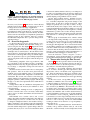
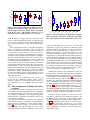
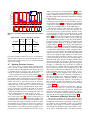
tuning parameters for different locations. The left graph in
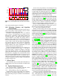
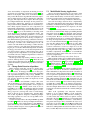
Figure 8 shows the basic statistics over the entire 6.5-hourlong temperature data, while the right one focuses on the
temperature under normal flow, excluding no-flow periods
PM
PM
PM
4:
58
3:
48
3:
05
PM
2:
35
1:
09
PM
240
PM
Figure 8. Two box-plots illustrate the difference in temperature between three location. The blue boxes cover
both the upper and lower quartile with a red median
mark in the center. The whiskers extend to 1.57 interquartile range, excluding outliers (red ’+’ marks).
4.5
260
T d2
:2
5
T d1
PM
Tu
12
T d2
:0
1
T d1
A
M
Tu
280
12
0
normal flow only
:0
1
all data
mote ADC
340
11
mote ADC
400
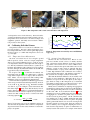
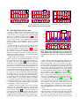
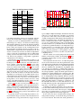
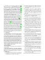
Figure 9. Box-plot illustrate the fluctuation of temperature when flow is normal at Tu during the experiment.
The x-axis tick labels are the starting time of each event.
caused by either pump-off or valve-close. We know that
temperatures of pipes vary, and they are affected by ambient temperature as well. With only one day for field experiments, we cannot allow the pipe to completely cool. In
addition, this statistics is not necessary because the overall and the normal-flow statistics are enough to prove that
temperatures vary. We find that the temperature upstream to
production-circulation branch-out (Tu ) is significantly different from the pair straddling the valve (Td1 and Td2 ), showing
by the different quartiles (blue boxes) in either plot. Hence,
auto-configuration is critical because one parameter setting
works on one location does not necessarily work on another.
For example, a reference value of 229 (ADC value) gives
100% accuracy on Tu , but would trigger three false positives
on sensor downstream to production valve (Td2 ).
Additional motivation for auto-configuration is that temperature changes constantly at the same location. Therefore
hand-tuning parameters on each sensor to cope with the location disparity is still insufficient. Figure 9 breaks down the
Tu temperature trace and compares between eight events only
when flow is normal. The temperature measurement fluctuation is significant, mostly caused by a noise combination
of diurnal amplitude, downhole change and back pressure
(Section 2.3). The first and last three boxes has no overlap with the other four, which suggests that maintaining a
fixed threshold during the whole time is likely to cause misdetections. Our further study confirm with this observation
and hence an adaptive temperature algorithm is necessary.
To address the above problems, our flow presence detection auto-configures the most important parameter—the
CUSUM reference value based on the training temperature under normal flows and pump shut-ins (details in Section 2.3). Our 100% accuracy shows it is effective (Section 4.4). More importantly, we find it is necessary because
if a uniform reference value were mis-configured above 229,
sensor downstream to production valve (Td2 ) would start to
trigger false positives.