Download SurvCalc manual 12March2012 - These are not the droids you are

SurvCalc
User Manual v1.2-2011-09-28
R.I.C.C. Francis
D. Fu
NIWA Technical Report 134
ISSN 1174-2631
March 2012
Published by NIWA
Wellington
2012
Enquiries to:
Science Communication, NIWA,
Private Bag 14901, Wellington, New Zealand
ISSN 1174-2631
© NIWA 2012
Citation:
Francis, R.I.C.C.; Fu, D. (2012). SurvCalc User Manual v1.2-2011-09-28.
. NIWA Technical Report 134. 54 p.
The National Institute of Water and Atmospheric Research
is New Zealand’s leading provider
of atmospheric, marine, and
freshwater science
Visit NIWA’s website at http://www.niwa.co.nz
Table of Contents
1.
INTRODUCTION ............................................................................................................. 5
1.1
Overview ................................................................................................................... 5
1.2
Relationship of SurvCalc to trawlsurvey ................................................................... 6
1.2.1
Extensions to trawlsurvey.................................................................................. 7
1.2.2
Excluded features of trawlsurvey ...................................................................... 7
1.2.3
Corrections to trawlsurvey ................................................................................ 7
1.3
Possible future extensions to SurvCalc ..................................................................... 8
2.
RUNNING SurvCalc ......................................................................................................... 9
3.
INPUT FILE SPECIFICATIONS ................................................................................... 10
3.1
The main input file .................................................................................................. 10
3.1.1
Commands defining the data ........................................................................... 11
3.1.2
Commands modifying the data ........................................................................ 14
3.1.3
Commands extending the data......................................................................... 16
3.1.4
Commands defining the calculations............................................................... 21
3.1.5
Commands defining output ............................................................................. 25
3.1.6
Examples of main input files ........................................................................... 27
3.1.7
Repeated commands in the main input file ..................................................... 31
3.2
4.
Other input files ....................................................................................................... 32
OUTPUT FILES .............................................................................................................. 33
4.1
Main output file ....................................................................................................... 33
4.1.1
4.2
5.
Tables in the main output file .......................................................................... 34
Output to flat files.................................................................................................... 36
4.2.1
Station-catch file.............................................................................................. 36
4.2.2
Output to stratum-catch file ............................................................................. 37
4.3
Catch-at-age data output .......................................................................................... 37
4.4
Precision of numbers in output files ........................................................................ 38
CALCULATIONS IN SurvCalc ..................................................................................... 39
5.1
Data and notation..................................................................................................... 39
5.1.1
Note on subcatches .......................................................................................... 41
5.1.2
Note on stations and strata without LF data .................................................... 41
5.1.3
Excluding stations and strata ........................................................................... 41
5.1.4
User preferences for fish-density variables ..................................................... 42
5.1.5
Calculation of c.v.s .......................................................................................... 42
5.1.6
Use of length-weight coefficients .................................................................... 42
5.2
Calculating fish densities......................................................................................... 43
5.3
Calculating biomasses ............................................................................................. 43
5.3.1
Calculating sub-population biomasses ............................................................ 43
3
5.4
5.4.1
Calculating LFs ....................................................................................................... 44
Calculating c.v.s for LFs ................................................................................. 45
5.5
Calculating phase-2 gains ........................................................................................ 46
5.6
Calculating projected c.v.s ...................................................................................... 47
5.7
Output for catch-at-age ............................................................................................ 48
6.
SurvCalc and 2-PHASE SURVEYS ............................................................................... 49
7.
REFERENCES ................................................................................................................ 51
8.
Appendix 1: Command block format ............................................................................. 52
9.
Appendix 2: The SurvCalc R library .............................................................................. 53
4
1.
INTRODUCTION
1.1 Overview
SurvCalc is a C++ computer program which analyses data from stratified random surveys. Its
primary purpose is to calculate estimates of biomass and/or length frequencies (LFs), and
associated coefficients of variation (c.v.s), from survey data. These data may be held either in
a database structured like the Ministry of Fisheries database trawl (Mackay 2000) or in flat
files. SurvCalc supersedes, and uses some code from, the program ‘trawlsurvey’ (Vignaux
1994).
Users of SurvCalc are urged to include their input files in an appendix to any report
describing the analysis of stratified random surveys. The main input file for SurvCalc has
been designed so that, taken together with this manual, it fully documents all the choices the
user makes in calculating biomass etc (e.g., the choice of stations to include, and how distance
towed is calculated if there is no recorded value). This will allow readers of survey reports to
replicate the analyses therein. When SurvCalc is run using data from flat files, rather than
from a database, these flat files should also be included in the report to complete the
documentation.
Each time SurvCalc is run it carries out one of the seven following tasks. The first three tasks
involve different types of calculations that may be made either during a survey or afterwards.
Each can be applied to analyse multiple species in multiple surveys (or trips) in a single run of
SurvCalc, and the species analysed may be different in different trips.
1. Task calc_biomass. Calculates biomasses, by stratum and overall. Can also calculate
biomasses for sub-populations defined by sex and/or length range (e.g., for males of length
between 20 cm and 80 cm). C.v.s are calculated for all biomasses. Optionally, calculates,
during a survey, projected biomass c.v.s (i.e., the c.v.s expected at the end of the survey given
the data to date – this can be useful during a 2-phase survey).
2. Task calc_LFs. Calculates LFs by station and/or stratum and/or overall. All LFs are
presented by sex (including a category for unsexed) and overall. The user can choose
between five alternative methods of scaling the LFs. C.v.s are not calculated for LFs.
3. Task calc_biomass_and LFs. Combination of tasks calc_biomass and
calc_LFs but only one method of LF scaling is allowed (scaling to represent estimated
numbers in the population) and c.v.s are optionally calculated for LFs by stratum and sex.
The next task will usually be used at sea at (or near) the end of phase 1 of a 2-phase survey
(Francis 1984). It can be applied only to a single trip (but can involve multiple species) and is
intended to provide information useful in deciding on the phase-2 allocation (i.e., how a
specified number of phase-2 stations should be allocated amongst the survey strata). Some
guidance on how SurvCalc should be used during a 2-phase survey is given in Section 6.
4. Task phase_2_calc. Calculates, separately for each species requested, the relative
gains (in terms of reduced variance of biomass estimates) associated with allocating varying
numbers of phase-2 stations in each stratum. From this information the optimum phase-2
allocation can be derived for each species.
The last three tasks simply reorganise the survey data and output it in a different form.
5. Task output_flat_files. Output data in one or more of seven types of flat file.
Depending on the type, each line of an output flat file may represent a stratum, a station, a
5
catch or subcatch record (i.e., a combination of a station and a species), or a length record
(i.e., a combination of station, species, subcatch, and length).
6. Task output_LW_coeffs. Output a table of length-weight coefficients. This shows
what length-weight coefficients are held in database rdb for each species so that the user can
decide whether to use these stored coefficients or to specify new coefficients. (See Section
5.1.6 for a description of how these coefficients are used in various calculations).
7. Task output_for_catch_at_age. Output a file (in either ‘survey’ or ‘survey.sub’
format, whichever is appropriate) for input to the catch-at-age software (Bull & Dunn 2002).
That is a file that can be read by the catch-at-age function import.length.data.
The remainder of this section compares SurvCalc with its predecessor, trawlsurvey, and
discusses some possible future extensions of SurvCalc. Sections 2 describes how to run
SurvCalc; Sections 3 and 4 describe the various input and output files, respectively; Section 5
documents the calculations in SurvCalc; and Section 6 discusses how SurvCalc output should
be used in 2-phase surveys.
1.2 Relationship of SurvCalc to trawlsurvey
This section is aimed at past users of the program trawlsurvey (Vignaux 1994) and may safely
be ignored by others. It is intended to help introduce these past users to the main features of
SurvCalc by comparing it with the earlier program.
From the user’s point of view a major difference between trawlsurvey and SurvCalc is the
way in which they define the analyses they want. For trawlsurvey this was done by entering
information via a series of blue screens, whereas for SurvCalc this information is written into
the main input file (in a command-block format similar to that for CASAL). This file,
together with the SurvCalc manual, will serve as a complete documentation of the analysis.
A second important difference concerns the computers on which each program will run and
their data requirements. trawlsurvey runs only on Unix machines and requires the survey data
to be in an Empress database structured like trawl (Mackay 2000). In contrast, SurvCalc runs
on both Unix and Windows machines and can access survey data either in flat files or in
Empress or Postgresql databases.
A third, more subtle, difference between the two programs is that the format of the output has
been tweaked so that it is easier to read it into R for plotting and further analysis (see
Appendix 2).
All the main calculations in trawlsurvey – of biomass and LFs – are exactly the same in
SurvCalc (in fact much trawlsurvey code was reused in SurvCalc). However, SurvCalc
includes several new features (see Section 1.2.1), discards a few features of trawlsurvey (see
Section 1.2.2), and corrects a couple of minor errors in that program (see Section 1.2.3).
Before describing these differences in functionality of the two programs it’s worth noting, for
the record, some technical programming differences. trawlsurvey is actually the combination
of two programs: an Empress 4GL interface, which is what the user sees (this generates all the
blue screens), and a C program, which is run, in batch mode, from that interface. SurvCalc is
a single C++ program.
6
1.2.1
Extensions to trawlsurvey
The following are the main features of SurvCalc that were not possible with trawlsurvey
(excluding those just mentioned).
– Biomass and LFs can be calculated for multiple trips and/or species in a single run.
– Data can be extracted from the trawl database and output in flat files of station data
(one line per station), stratum data (one line per stratum), catch data, and length data.
– Input files for use in the catch-at-age software can be output
– The analysis of potting surveys is more straightforward and sensible (i.e., the user will
not have to make up fake values for doorspread and distance towed).
– Sex-specific length-weight coefficients are allowed.
– The calculations for phase 2 of a 2-phase survey are much more extensive (see Section
6).
– The user can control the degree of precision (expressed as the number of significant
figures and/or decimal places) of each type of output.
1.2.2
Excluded features of trawlsurvey
1. trawlsurvey produces LFs as percentages (in the main output file) and as numbers (in
separate files, but some summary information for the numbers LFs is, confusingly, included
in the main output file). SurvCalc produces LFs only as numbers (LFs as percentages are
easily calculated from these).
2. SurvCalc does not allow the user to define bounds and interval for LFs (e.g., for lengths 20
cm to 50 cm in 2 cm steps). All SurvCalc LFs cover the full range of the data in 1-cm steps.
The length bounds are not well handled in trawlsurvey: it is not made clear that (oddly) they
apply to the percentage LFs and (confusingly) the summaries of the numbers LFs, but not to
the numbers LFs; also, the user is not informed when there are length data outside the
specified length bounds.
3. trawlsurvey outputs a table containing, inter alia, mean fish densities and biomass
estimates by stratum, where the density units – kg/km and kg/km2 – are chosen by the user,
although the biomass estimates are always based on densities in kg/km2. This is potentially
misleading because the obvious inference from this table is that the biomass estimates derive
from the presented densities. In SurvCalc, the densities in this table are always in kg/km2 (but
kg/km can be calculated, if requested, and output to separate station-catch and/or stratumcatch files).
1.2.3
Corrections to trawlsurvey
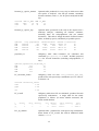
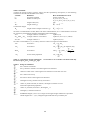
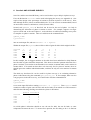
1. LFs for stations and species with more than one subcatch are not well handled in
trawlsurvey. For such stations there can be more than one record in the trawl table t_lgth
with the same station_no, species, and lgth, as in the following extract.
7
trip_code
tan0601
tan0601
station_no
79
79
species
HOK
HOK
subcatch_no
1
2
lgth
56
56
percent_samp
5.53
10.55
no_a
2
8
In trawlsurvey this will, misleadingly, produce two lines for length 56 cm in the LF for station
79 (but there’s no problem with stratum and overall LFs). This does not occur with SurvCalc.
2. Although the trawlsurvey blue screen says that there should be no overlap in the length
ranges of sub-populations, the program actually does allows overlap, and sometimes this
causes errors (e.g., when, accidentally, two identical length ranges were specified,
trawlsurvey produced just one sub-population biomass for this length range but this biomass
was too high by a factor of 2). SurvCalc allows overlap in length ranges and treats these
correctly.
1.3 Possible future extensions to SurvCalc
This section describes features that may be incorporated in future versions of SurvCalc,
depending on demand from users (and the coding effort required).
1. SurvCalc could be extended to analyse survey data in databases like scallop and oyster.
The structures of these databases are broadly similar to trawl, but with some relatively minor
differences that would have to be allowed for.
2. When designing new trawl surveys, there is a need to decide, on the basis of previous
survey data, how many stations need to be allocated to each stratum to achieve a target c.v..
One way this is currently done is in the following two steps: (a) extract data from previous
surveys in the trawl database, and (b) run the Splus function allocate (see Appendix 2). It
might be useful to combine these two steps in SurvCalc.
3. SurvCalc allows the calculation of biomasses of sub-populations defined by sex and length
(e.g., all males less than 30 cm long). This could be extended to allow the use of gonad-stage
data in defining sub-populations (e.g., all females of stage > 2). This would involve using
trawl tables t_fish_bio and/or t_lgth_stage, not currently used by SurvCalc.
4. SurvCalc could calculate length-weight coefficients for a species in a survey (or surveys).
Ideally, this calculation should (a) be robust to outliers, (b) include graphical output to show
the user how well the data fit the estimated curve and what range of lengths is well covered
by the relationship, and (c) include the ability to test for significant differences between the
parameters for males and females.
5. Some users have asked for the ability to calculate total biomass for large groups of species
(e.g., ‘all fish’, which means excluding invertebrates etc). This might involve using the
attribute descrptn in table species_master in database rdb to define groups of species.
6. Current options for LF scaling make no allowance for correlation in the samples (i.e., the
fact that, typically, the lengths of two fish from the same tow are more similar than those from
different tows). When more sophisticated scaling schemes are developed they should be
available in SurvCalc.
8
2. RUNNING SURVCALC
SurvCalc is run from the command prompt (in Windows or Unix) by typing a command like
SurvCalc -b -t stnfile > myfile. It uses information from the main input file and
possibly some flat files (all described in Section 3), makes certain calculations (documented
in Section 5), and writes results to the main output file (myfile in the preceding example),
and possibly other files (see Section 4). In the command line, between SurvCalc and >,
there must be one or more run-time arguments (which may occur in any order) as described
below.
The command line must include exactly one of following run-time arguments, which
describes the task required of SurvCalc:
Argument
-b
-l
-B
-2
Task
calc_biomass
calc_LFs
calc_biomass_and LFs
phase_2_calc
-o output_flat_files
-p output_LW_coeffs
-c output_for_catch_at_age
-h help
-L show license
Task description
calculate biomass
calculate LFs
calculate biomass and LFs
do calculations for allocating phase-2 stations in a
2-phase survey
only output flat files of data (to be used only in
conjunction with arguments -s, -t, -u, or -v)
output a table of length-weight coefficients (from
database rdb)
output a file (in either ‘survey’ or ‘survey.sub’
format, whichever is appropriate) for input to the
catch-at-age software
list all arguments
display the SurvCalc end user license
In addition, one or more of the following run-time arguments can be used to provide
information about input and output files:
Argument
-S [infile]
-T [infile]
-U [infile]
-V [infile]
-W [infile]
-X [infile]
-s [outfile]
-t [outfile]
-u [outfile]
-v [outfile]
Description
read stratum data from a flat file rather than a database; default value for
infile is stratum.in
read station data from a flat file rather than a database; default value for
infile is station.in
read catch data from a flat file rather than a database; default value for
infile is catch.in
read length data from a flat file rather than a database; default value for
infile is lgth.in
read subcatch data from a flat file rather than a database; default value for
infile is subcatch.in
read combined station and catch rate data from a flat file rather than a
database; default value for infile is station_catch.in
output a flat file of stratum data (one line per stratum); default value for
infile is stratum.out
output a flat file of station data (one line per station); default value for
outfile is station.out
output a flat file of catch data (one line per catch record); default value
for outfile is catch.out
output a flat file of length data (one line per length record); default value
for outfile is lgth.out
9
-w [outfile]
-x [outfile]
-y [outfile]
-f infile
output a flat file of subcatch data (one line per subcatch record); default
value for outfile is subcatch.out; to be used only with -o
output a flat file of combined station, catch, and catch rate data (one line
per station); default value for outfile is station_catch.out; to be used
only with -b, -B, or -l
output a flat file of combined stratum, catch, and catch rate data (one line
per stratum); default value for outfile is stratum_catch.out; to be
used only with -b, -B, or –l
alternative name for the main input file (e.g., -f ORH.slc means that
the main input file will be ORH.slc rather than the default input.slc)
SurvCalc obtains the data to be analysed either from an (Empress or PostgreSQL) database, or
from flat files (-S, -T,-U,-V, -W, and -X), but not both (e.g., you cannot provide station and
stratum flat files but expect SurvCalc to get catch and length data from the database). The flat
files that need to be provided depend on the run time task and some of the preferences
specified in the input file (e.g., biomass calculation involving no sub-populations and using
the ‘recorded’ catch preference requires stratum (-S), station (-T), and catch data files (-U), or
alternatively stratum (-S) and station-catch (-X) data files). SurvCalc will give error messages
if data provided are inconsistent with the run time task and preferences.
3.
INPUT FILE SPECIFICATIONS
SurvCalc requires a main input file (described in Section 3.1) which describes the data that
are to be analysed and specifies some details of the analyses and the desired output. The
actual data to be analysed are read either from an (Empress or PostgreSQL) database or from
user-provided flat files (described in Section 3.2).
3.1 The main input file
The main input file for SurvCalc has default name input.slc (but this name can be changed
if run-time argument -f is used – see Section 2). It uses a command-block format similar to
that used in CASAL. The order of command blocks within the main input file, and of
subcommands within a command block, is arbitrary (other conventions of this format are
described in Appendix 1).
The commands used in the main input file fall into five categories, depending on their
function, as follows.
Commands defining the data (Section 3.1.1). What data are to be analysed: what type of
survey (trawl or pot); which trip and species are to be analysed; which stations to use
from that trip; which database (if any) should be accessed and what additional data
should be extracted.
Commands modifying the data (Section 3.1.2). What changes should be made to the data
extracted from the database: stations can be reassigned to different strata (either
existing ones, or new user-defined strata); areas of existing strata can be changed.
Commands extending the data (Section 3.1.3). Non-database information needed for the
analyses: vulnerability and vertical availability for each station; areal availability for
each stratum; area fished (for pot surveys); length-weight coefficients.
10
Commands defining the calculation (Section 3.1.4). User’s preference for various options
in the calculations: how should the distance towed at each station be calculated (from
start and finish positions, or from recorded speed and time, etc.); what should be the
width swept at each station (the recorded doorspread or a specified constant); what subpopulations, if any, should biomass be calculated for; how should LFs be scaled;
information needed for phase-2 calculations and projected c.v.s.
Commands defining output (Section 3.1.5). What tables should be included in the output
file and what degree of precision should be used for different categories of output (fish
density, biomass, LF numbers, c.v., gain)?
Some examples of main input files are given in Section 3.1.6. Commands that may be (and
sometimes must be) repeated in the main input file are discussed in Section 3.1.7.
3.1.1
Commands defining the data
The commands in this section define what type of survey is to be analysed (trawl or pot),
which trip(s) and species are to be analysed, whether the data are to be read from a database
or flat files and, if the former, which stations to use from the specified trip(s).
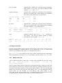
If the data are to be read from a database, some of all of the data in Table 1 will be extracted.
Which tables are extracted depends on the specific analysis.
Table 1: Database tables from which data may be extracted by SurvCalc, and the attributes
extracted from each table. The database and table names given are those for the original
implementation (on Empress at Greta Point); slightly different names might apply in other
situations.
Database
trawl
trawl
Table
t_stratum
t_station
Attributes extracted
trip_code, stratum, area_km2
trip_code, station_no, stratum, distance, lat_s, NorS_s, long_s, EorW_s,
lat_s, NorS_f, long_f, EorW_f, speed, dist_doors and any other
attributes included in @input_from_database.t_station_columns
trawl
t_catch
trip_code, station_no, species, weight
trawl
t_subcatch1
trip_code, station_no, species, subcatch_no, weight
trawl
t_lgth
trip_code, station_no, species, subcatch_no2, lgth, percent_samp, no_a,
no_m, no_f
rdb
lw_coeff
spp_code, sex lw_coeff_a, lw_coeff_b, lw_coeff_c
1
This table extracted only for task output_for_catch_at_age (see Section 5.7)
2
This attribute extracted only for task output_for_catch_at_age (see Section 5.7)
@survey_type
Type
Default
Effects
Notes
@trips
Type
Effects
Type of survey
String (must be either trawl or pot)
trawl
Determines which alternative variables and equations will be used in
calculations and what other input file commands are valid. Other types of
survey that may be allowed in future versions of SurvCalc include scallop
and oyster.
This command is not needed for trawl surveys.
The trip, or trips, that should be analysed
String vector, each member of which must be a valid trip code
Limits the data extracted from the database to that relating to the specified trip
or trips
11
@species
Label
Effects
Notes
codes
Command
Conditions
Type
Effects
The species to be analysed for a specified trip
A trip code (must be in the vector trips)
Defines any following subcommands as being @species subcommands for
the specified trip
Omit the label if only one trip is being analysed (i.e., if trips is of length 1).
Species codes
@species
Only one species can be analysed (i.e., codes must have length 1) if the task
is output_for_catch_at_age.
String vector, each member of which must be a valid species code
Limits the catch and/or length data extracted from the database for the
specified trip to that relating to the specified species.
@input_from_database The interface to the database to extract the data
Effects
Defines any following subcommands as being @input_from_database
Notes
Ignored if the user has provided flat file input data (with run-time
arguments -S, -T, -U, -V, or -W)
database
Command
Conditions
Type
Default
Effects
database
@input_from_database
Either Empress or Postgresql
String
Empress
Specifies the database from which the data are to be extracted.
hostname
Command
Conditions
Postgresql server name
@input_from_database
Only used for Postgresql database, and only needed when this database is
being accessed across a network (i.e., when SurvCalc is not running on the
machine on which the Postgresql database resides)
String
Specifies the machine name on which the Postgresql database resides.
Type
Effects
schema
Command
Conditions
Type
Default
Effects
schema name
@input_from_database
Only used for Postgresql database
String
trawl
Specifies the Postgresql schema name under which data tables are stored.
database_name
Command
Type
Default
Effects
database name
@input_from_database
String
trawl for Empress or fish for Postgresql
Specifies the database name in which data tables are stored.
t_station_columns
Command
Type
Conditions
Effects
the additional attributes to be extracted from t_station table
@input_from_database
String vector
The attributes must exist in t_station table of the database
Specifies the additional attributes to be extracted from t_station table.
12
@where
Label
Effects
Notes
Example
Restrict the selects from the database tables
A trip code (must be in the vector trips)
Restricts the records selected from one or more of database tables t_stratum,
t_station, t_catch, and t_lgth. Defines any following subcommands as being
@where subcommands for the specified trip.
Most users will want to use only subcommand t_station (to define the
station select). The label may be omitted if only one trip is being analysed
(i.e., if trips is of length 1).
The following command block restricts the stations selected to those for which
gear_perf is less than 3 and station_no is less than 100
@where
t_station gear_perf < 3 and station_no < 100
t_station
Command
Type
Effects
Notes
Restrictions for extracting station data
@where
String (must be a valid SQL Boolean expression)
Specifies criteria to restrict the selection of station data from t_station table.
SurvCalc automatically constructs an SQL to extract data from table t_station,
and this ends with a ‘where’ clause restricting this extraction to the specified
trip(s). SurvCalc will append t_station to this ‘where’ clause using ‘and’.
t_stratum
Command
Type
Effects
Notes
Restrictions for extracting stratum data
@where
String (must be a valid SQL Boolean expression)
Specifies criteria to restrict the selection stratum data from t_stratum table.
SurvCalc automatically constructs an SQL to extract data from table t_stratum,
and this ends with a ‘where’ clause restricting this extraction to the specified
trip(s). SurvCalc will append t_stratum_where to this ‘where’ clause
using ‘and’.
t_catch
Command
Type
Effects
Notes
Restrictions for extracting catch data
@where
String (must be a valid SQL Boolean expression)
Specifies criteria to restrict the selection catch data from t_catch table.
SurvCalc automatically constructs an SQL to extract data from table t_catch,
and this ends with a ‘where’ clause restricting this extraction to the specified
trip(s) and species. SurvCalc will append t_catch_where to this ‘where’
clause using ‘and’.
t_lgth
Command
Type
Effects
Notes
Restrictions for extracting length data
@where
String (must be a valid SQL Boolean expression)
Specifies criteria to restrict the selection catch data from t_lgth table.
SurvCalc automatically constructs an SQL to extract data from table t_lgth,
and this ends with a ‘where’ clause restricting this extraction to the specified
trip(s) and species. SurvCalc will append t_lgth_where to this ‘where’
clause using ‘and’.
13
3.1.2
Commands modifying the data
The commands in this section allow the user to modify the stratification in the data that have
been read in (either from a database or flat files). The following changes can be made:
stations can be reassigned to different strata (either existing ones, or new user-defined strata);
and areas of existing strata can be changed.
@change_strata
Label
Conditions
Effects
Notes
Examples
Reassign all stations in some strata to different strata (new or existing)
A trip code (must be in the vector trips)
It is a fatal error if there is any overlap between the stations affected by a
@change_strata command and a @reassign_strata command for
the same trip.
Defines any following subcommands as being @change_strata
subcommands for the specified trip. All stations from the specified trip that
were originally assigned to one of the strata listed in to are reassigned to the
corresponding stratum in from
Omit the label if only one trip is being analysed (i.e., if trips is of length 1).
The following example assigns all stations in stratum 0023 or 0025 to stratum
023A and all stations in stratum 0027 to stratum 0030
@change_strata
from
0023 0025 0027
to
023A 023A 0030
from
Command
Conditions
Type
Names of strata whose stations are to be reassigned
@change_strata
Each string in from must be an existing stratum name for the specified trip
String vector
to
Names of strata to which stations are to be reassigned
@change_strata
Each string in must be either an existing stratum or defined in command
@new_strata (i.e., must be in new_strata[trip].names)
String vector of same length as from
Command
Conditions
Type
@reassign_strata
Label
Conditions
Effects
Notes
Examples
stations
Command
Conditions
Type
Reassign some stations to different strata (new or existing)
A trip code (must be in the vector trips)
It is a fatal error if there is any overlap between the stations affected by a
@change_strata command and a @reassign_strata command for
the same trip.
Defines any following subcommands as being @reassign_strata
subcommands for the specified trip. Each station in stations is reassigned
to the corresponding stratum in strata
Omit the label if only one trip is being analysed (i.e., if trips is of length 1).
In the following example station 23 is reassigned to stratum 0012 and station
37 to stratum 012A
@reassign strata tan0601
stations 23 37
strata 0012 012A
Numbers of those stations which are to be reassigned to different strata
@reassign_strata
Each number in stations must be an existing station number for the
specified trip
Integer vector
14
strata
Command
Conditions
Type
@new_strata
Label
Effects
Notes
Example
Names of the strata to which stations are to be reassigned
@reassign_strata
Each string in strata must be an existing stratum name for the specified trip
or must be defined in command @new_strata (i.e., must be in
new_strata[trip].names)
String vector
Define new strata
A trip code (must be in the vector trips)
Defines any following subcommands as being @new_strata subcommands
for the specified trip.
Omit the label if only one trip is being analysed (i.e., if trips is of length 1).
Areal availabilities for the new strata will be assumed to be 1. Different
values, which are trip- and species-specific, may be set using command
@areal_availability
The following command creates new strata 003A and 003B for trip tan0601
with areas 2153 and 397, respectively, and areal-availabilities 1 and 0.8,
respectively
@new_strata tan0601
strata 003A 003B
areas 2153 397
strata
Command
Conditions
Type
Effects
Notes
Names of new strata
@new_strata
Must be different from the names of existing strata
String vector
Defines the names of new strata
A warning should be output if any string in names does not occur in either
change_strata[trip].to or reassign_strata[trip].strata
areas
Command
Type
Effects
Notes
Area (km2) of each new stratum
@new_strata
A numeric vector of the same length as names
Defines the areas of new strata
@change_stratum_area Change the areas of existing strata
Label
A trip code (must be in the vector trips)
Effects
Defines any following subcommands as being @change_stratum_area
subcommands for the specified trip. Changes the area of the strata with
names in names to the values in new_areas
Notes
Omit the label if only one trip is being analysed (i.e., if trips is of length 1).
Example
The following command block changes the area of strata 004A and 004B to
3152 and 793, respectively
@change_stratum_area tan0601
strata 004A 004B
new_areas 3152 793
strata
Command
Conditions
Type
Names of strata whose areas are to be changed
@change_stratum_area
Must be names of existing strata
String vector
new_areas
Command
Type
New areas for strata whose areas are to be changed
@change_stratum_area
Numerical vector
15
3.1.3
Commands extending the data
The commands in this section allow the user to extend the data to be analysed by providing
length-weight coefficients or setting the multiplicative factors which affect either the
calculation of fish density (vulnerability, vertical availability, and area fished – see Section
5.2) or the calculation of biomass from fish density (areal availability or population area – see
Section 5.3). Length-weight coefficients need be provided only if they are needed (see
Section 5.1.6) and if the default values in the database are not present or correct. Most of the
multiplicative factors have default values (1 for vulnerability and both areal and vertical
availability; the stratum area for population area). Other values must be provided separately
for each combination of trip and species. Note that vulnerability, vertical availability, and
area fished are associated with stations; areal availability and population area are associated
with strata.
@vulnerability
Label
Conditions
Effects
Notes
Examples
Vulnerability of a species to capture at each station in a trip
[trip_code]_[species_code]
Ignored if the user has provided station-catch data (-W). Must not be used
when survey_type = pot
Defines any following subcommands as being @vulnerability
subcommands. Specifies a vulnerability for the given species at all stations in
the given trip.
Each @vulnerability command block applies to one species in one trip.
The command may be omitted when the vulnerability of the species is 1 at all
stations in the trip.
The following command block specifies that the vulnerability of HOK in trip
tan0601 is 0.9 and 0.8 for stations 23 and 25, respectively, and 1 for all other
stations.
@vulnerability tan0601_HOK
default_value 1
other_stations 23 25
other_values 0.9 0.8
default_value
Command
Type
Default
Effects
Default value for vulnerability of the given species in the given trip
@vulnerability
Positive number
1
Defines the vulnerability of the given species in all stations in the given trip
except for those in other_stations
other_stations
Command
Conditions
Type
Effects
Stations at which the vulnerability differs from the default value
@vulnerability
Must be existing stations
Numeric vector
Specifies stations at which the vulnerability differs from the default value
other_values
Command
Type
Effects
Vulnerability values that differ from the default value
@vulnerability
Positive numeric vector of same length as other_stations
Specifies the vulnerabilities for those stations in other_stations
16
@vertical_availability Vertical availability of a species at each station in a trip
Label
[trip_code]_[species_code]
Conditions
Ignored if the user has provided station-catch data (-W). Must not be used
when survey_type = pot.
Effects
Defines
any
following
subcommands
as
being
@vertical_availability subcommands.
Specifies a vertical
availability for the given species at all existing stations in the given trip.
Notes
Each @vertical_availability command block applies to one species
in one trip. The command may be omitted when the vertical availability of the
species is 1 at all stations in the trip.
Examples
The following command block specifies that the vertical availability of HOK
in trip tan0601 is 0.8 and 1.2 for stations 33 and 35, respectively, and 1 for all
other stations.
@vertical_availability tan0601_HOK
default_value 1
other_stations 33 35
other_values 0.8 1.2
default_value
Command
Type
Default
Effects
Default value for vertical availability of the given species in the given trip
@vertical_availability
Positive number
1
Defines the vertical availability of the given species in all stations in the given
trip except for those in other_stations
other_stations
Command
Conditions
Type
Effects
Stations at which the vertical availability differs from the default value
@vertical_availability
Must be existing stations for the given trip
Numeric vector
Specifies stations at which the vertical availability differs from the default
value
other_values
Command
Type
Effects
Vertical availability values that differ from the default value
@vertical_availability
Positive numeric vector of same length as other_stations
Specifies the vertical availabilities for those stations in other_stations
@area_fished
Label
Conditions
Effects
Notes
Examples
default_value
Command
Type
Default
Effects
Area fished (m2) for a species at each station in a potting survey
[trip_code]_[species_code]
Must not be used except when survey_type = pot.
Defines any following subcommands as being @area_fished
subcommands. Specifies an area fished for the given species at all existing
stations in the given trip.
Each @area_fished command block applies to one species in one trip.
The following command block specifies that the area fished for BCO in trip
abc0601 is 27 m2 and 25 m2 for stations 33 and 35, respectively, and 30 m2 for
all other stations.
@area_fished abc0601_BCO
default_value 30
other_stations 33 35
other_values 27 25
Default value for area fished for the given species in the given trip
@area_fished
Positive number
None
Defines the area fished for the given species at all stations in the given trip
except for those in other_stations
17
other_stations
Command
Conditions
Type
Effects
Stations at which the area fished differs from the default value
@area_fished
Must be existing stations for the given trip
Numeric vector
Specifies stations at which the area fished differs from the default value
other_values
Command
Type
Effects
Area fished values that differ from the default value
@area_fished
Positive numeric vector of same length as other_stations
Specifies the areas fished for those stations in other_stations
@areal_availability
Label
Conditions
Effects
Notes
Examples
Areal_availability of a species at each stratum in a trip
[trip_code]_[species_code]
For each combination of trip and species to be analysed there must not be both
an @areal_availability command block and a @population_area
command block (use one or the other, or neither).
Defines any following subcommands as being @areal_availability
subcommands. Specifies an areal availability for the given species at all
existing strata in the given trip.
Each @areal_availability command block applies to one species in
one trip. The command may be omitted when the areal availability of the
species is 1 at all strata in the trip.
The following command block specifies that the areal availability of HOK in
trip tan0601 is 0.8 and 1.2 for strata 0003 and 0004, respectively, and 1 for all
other strata.
@areal_availability tan0601_HOK
default_value 1
other_strata 0003 0004
other_values 0.8 1.2
default_value
Command
Type
Default
Effects
Default value for areal availability of the given species in the given trip
@areal_availability
Positive number
1
Defines the areal availability of the given species in all strata in the given trip
except for those in other_strata
other_strata
Command
Conditions
Type
Effects
Strata in which the areal availability differs from the default value
@areal_availability
Must be existing strata for the given trip
String
Specifies strata in which the areal availability differs from the default value
other_values
Command
Type
Effects
Areal availability values that differ from the default value
@areal_availability
Positive numeric vector of same length as other_strata
Specifies the areal availabilities for those strata in other_strata
18
@population_area
Label
Conditions
Effects
Notes
Examples
Population area for species in each stratum in a trip
[trip_code]_[species_code]
For each combination of trip and species to be analysed there must not be both
an @areal_availability command block and a @population_area
command block (use one or the other, or neither).
Defines any following subcommands as being @population_area
subcommands. Specifies a population area for the given species at all existing
strata in the given trip. This is used to calculate areal availability, which is
population area divided by stratum area
Each @population_area command block applies to one species in one
trip. The command may be omitted when the population area of the species is
the same as the stratum area for all strata in the trip.
The following command block specifies that the population area of HOK in
trip tan0601 is 2957 and 1325 for strata 0003 and 0004, respectively, and
equal to the stratum area for all other strata.
@population_area
other_strata 0003 0004
other_values 2957 1325
other_strata
Command
Conditions
Type
Effects
Strata in which the population area differs from the stratum area
@population_area
Must be existing strata for the given trip
String
Specifies strata in which the population area differs from the stratum area
other_values
Command
Type
Effects
Population areas that differ from stratum area
@population_area
Positive numeric vector of same length as other_strata
Specifies the population area for those strata in other_strata
@lw_coeff
Label
Conditions
Effects
Notes
Examples
a, b, c
Command
Conditions
Type
Default
Length-weight coefficients for a species in a trip
[trip_code]_[species_code]
Needed only if length-weight coefficients are required for an analysis and the
user wants to use values different from those in database rdb. If this
command is used it must be repeated for each combination of trip and species
for which length-weight coefficients are required (see Section 5.1.6). If it is
not used, then all required length-weight coefficients will be read from rdb.
Defines any following subcommands as being @lw_coeff subcommands.
Specifies the coefficients used to calculate the weight of a fish (in g) from its
length (in cm).
Note that length-weight coefficients are not always required in analyses (see
Section 5.1.6).
The following command block specifies the length-weight coefficients
(independent of sex) for HOK in trip tan0601.
@lw_coeff tan0601_HOK
a 0.006
b 2.85
Length-weight coefficients [to calculate the weight of a fish (in g) from its
length (in cm)].
@lw_coeff
Use either a, b, and (optionally) c, or a_male, b_male, a_female,
b_female, and (optionally) c_male, c_female, a_unsexed,
b_unsexed, c_unsexed
Numeric
c = 1; no default for a or b
19
a_male, b_male, c_male, a_female, b_female, c_femaleLength-weight coefficients by sex [to
calculate the weight of a fish (in g) from its length (in cm)].
Command
@lw_coeff
Conditions
Use either a, b, and (optionally) c, or a_male, b_male, a_female,
b_female, and (optionally) c_male, c_female, a_unsexed,
b_unsexed, c_unsexed
Type
Numeric
Default
c_male = 1 and c_female = 1; no default for other coefficients
a_unsexed, b_unsexed, c_unsexed Length-weight coefficients for unsexed [to calculate the
weight of a fish (in g) from its length (in cm)].
Command
@lw_coeff
Conditions
Use either a, b, and (optionally) c, or a_male, b_male, a_female,
b_female, and (optionally) c_male, c_female, a_unsexed,
b_unsexed, c_unsexed
Type
Numeric
Default
c_unsexed = 1; no default for other coefficients
Notes
If length-weight coefficients are presented for males and females, but not for
unsexed fish, then the weight of an unsexed fish of a given length is calculated
as the average of the weights of a male and female of that length.
20
3.1.4
Commands defining the calculations
The commands in this section describe the user’s preference for various options in the
calculations. There are options associated with fish density (see Section 5.1.4), subpopulations defined by sex and/or length ranges (see Section 5.3.1), and the scaling of LFs
(see Section 5.4).
@preferences
Label
Conditions
Effects
Notes
distance_towed
Command
Conditions
Type
Default
Effects
Notes
width_swept
Command
Conditions
Type
Default
Effects
Notes
catch_weight
Command
Type
Default
Effects
Notes
User preferences for fish density calculations
A trip code (must be in the vector trips)
Ignored if: the task is output_lw_coeff; or if it is calc_LFs and
LF_scaling is not numbers_per_km2; or if the user has provided
station-catch data (-W).
Defines any following subcommands as being @preferences
subcommands for the specified trip.
Omit the label if only one trip is being analysed (i.e., if trips is of length 1).
User preference for calculation of distance towed at each station
@preferences
Must not be used when survey_type = pot
String vector containing one or more of the following options in order of
preference:
recorded_distance,
recorded_speed*time,
constant_speed*time, from_lat_lon
None
Defines the user preference for the method (or methods, in priority order) of
defining the distance towed at each station. Any station for which distance
towed can not be defined will be dropped from the analysis.
See Section 5.1.4 for more details about the options for distance_towed
User preference for defining width swept at each station
@preferences
Must not be used when survey_type = pot
String vector containing one or more of the following options in order of
preference:
recorded_doorspread,
constant_doorspread,
recorded_wingspread
None
Defines the user preference for the method (or methods, in priority order) of
defining the width swept at each station. Any station for which width swept
can not be defined will be dropped from the analysis.
See Section 5.1.4 for more details about the options for width_swept
User preference for calculation of catch weight at each station
@preferences
String vector containing one or more of the following options in order of
preference: recorded, calculated
None
Defines the user preference for the method (or methods, in priority order) of
defining the catch weight at each station. Any station for which catch weight
can not be defined will be dropped from the analysis.
See Section 5.1.4 for more details about the options for catch_weight
21
@sub_populations
Label
Conditions
Effects
Notes
Examples
sub-populations for which biomasses should be calculated
A species code (must be in species[trip].code for some trip in
trips)
Ignored
unless
the
task
is
one
of
calc_biomass,
calc_biomass_and_LFs, or phase_2_calc.
Defines any following subcommands as being @sub_populations
subcommands for the specified species.
For analyses covering more than one trip this command will affect the output
for the given species in all trips where that species is analysed.
The following command requests ORH biomass estimates for six subpopulations, and supplies labels to be used for these in the output file:
@sub_populations ORH
sexes
all all male male female female
Lmin
0
20
0
20
0
20
Lmax
20
80
20
80
20
80
labels A_sm A_lg M_sm M_lg
F_sm
F_lg
sexes
Command
Type
Effects
Sexes of sex-based sub-populations
@sub_populations
String vector containing one or more of all, male, female, and unsexed
Specifies the sex of each sub-population for the given species
Lmin, Lmax
Command
Type
Effects
Notes
Length bounds for each length-based sub-population
@sub_populations
Numeric vector of same length as sexes
Specifies length bounds for each sub-population for the given species
Sub-population includes all fish with Lmin ≤ length < Lmax
labels
Command
Type
Effects
User-supplied labels for sex-based sub-populations
@sub_populations
String vector of same length as sexes
Supplies labels for sub-population biomass estimates in the output
@constant_speed
Label
Conditions
Effects
Notes
value
Command
Type
Notes
Vessel speed to be used in calculating distance-towed
A trip code (must be in the vector trips)
Ignored if the user has provided station-catch data (-W). This command must
be provided for all trips in which constant_speed*time occurs in
preferences[trip]distance_towed. It will be ignored for other
trips.
Defines any following subcommands as being @constant_speed
subcommands for the specified trip.
Omit the label if only one trip is being analysed (i.e., if trips is of length 1).
User-supplied vessel speed for the given trip
@constant_speed
Number
This vessel speed will be used only for those stations in the specified trip in
which constant_speed*time is the selected option for calculating
distance towed (as specified in command @preferences)
22
@constant_doorspread Doorspread to be used in calculating the width swept
Label
A trip code (must be in the vector trips)
Conditions
Ignored if the user has provided station-catch data (-W). This command must
be provided for all trips in which constant_doorspread occurs in
preferences[trip]width_swept. It will be ignored for other trips.
Effects
Defines any following subcommands as being @constant_doorspread
subcommands for the specified trip.
Notes
Omit the label if only one trip is being analysed (i.e., if trips is of length 1).
value
Command
Type
Notes
User-supplied vessel doorspread for the given trip
@constant_doorspread
Number
This doorspread will be used only for those stations in the specified trip in
which constant_doorspread is the selected option for calculating width
swept (as specified in command @preferences)
@LF_scaling
Conditions
Method of scaling LFs
Ignored unless LFs are being calculated (i.e., the task is
calc_biomass_and_LFs
or
calc_LFs).
Option
numbers_in_population
is
obligatory
if
the
task
is
calc_biomass_and_LFs, and not allowed if it is calc_LFs.
String (must be one of unscaled,
numbers_per_1000,
numbers_per_tow,
numbers_per_hour,
numbers_per_km2,
numbers_in_population)
numbers_in_population in –B run, no default in –l run
Defines how LFs are scaled (see Section 5.4)
This command applies to all trips and species analysed. It can be omitted if
the task is calc_biomass, in which case there is only one LF_scaling
option.
Type
Default
Effects
Notes
@phase_2
Label
Conditions
Effects
Notes
User preferences for phase-2 gain calculations
A species code (must be in species[trip].code)
Ignored unless the task is phase_2_calc.
Defines any following subcommands as being @phase_2 subcommands.
If this command is used after some phase-2 stations have already been carried
out then you should use command @where to exclude these stations from this
analysis. It is not necessary to specify a trip for the phase-2 calculations
because it is a fatal error to request phase_2_calc when trips is of
length > 1.
algorithm
Command
Type
Default
Effects
Notes
Algorithm to be used in calculating gains
@phase_2
String (must be either mean_squared or variance).
mean_squared
Defines which algorithm will be used in calculating gain (see Section 5.5).
This sub-command is included only for completeness. Users should omit it
unless they have a very good reason to use the variance algorithm.
n_stations
Command
Type
Default
Effects
Maximum number of additional stations per stratum
@phase_2
Positive integer
None
Defines the maximum number of additional stations in each stratum for which
gains will be calculated (i.e., the number of columns in the output table of
gains – see Section 5.5).
23
@projected_cvs
Conditions
Effects
Example
Calculate projected biomass c.v.s during a survey
Ignored
unless
run_time
task
is
calc_biomass
or
calc_biomass_and_LFs. Can only be used in a single-trip analysis.
Calculates the projected biomass c.v.s (i.e., the c.v.s expected at the end of the
survey, given the data to date – see Section 5.6). Defines any following
subcommands as being @projected_cvs subcommands.
The following command block could be used during a 2-phase survey at the
time when all stations had been completed except for 2 in stratum 002A and 3
in stratum 002B.
@projected_cvs
strata
002A 002B
extra_stations
2
3
strata
Command
Conditions
Type
Effects
Strata that are not yet completed
@projected_cvs
There must already be at least two stations in all strata specified here
String vector of stratum names
Specifies which strata are not yet completed (i.e., those in which there are still
some more stations to be done)
extra_stations
Command
Type
Effects
Number of additional stations per stratum
@projected_cvs
Constant vector of same length as strata
Specifies how many more stations are to be done in each stratum named in
subcommand strata
24
3.1.5
Commands defining output
The main output file produced by SurvCalc contains obligatory and optional elements. The
commands in this section, together with command @station_data_columns in Section
3.1.1, allow the user to specify which optional elements should be included. They also
specify to what precision certain numbers (in both the main and other output files) should be
given.
@output_tables
Label
Conditions
Effects
Notes
Examples
Tables to include in the main output file
None
Ignored unless biomass or LFs are being calculated (i.e., the task is
calc_biomass, calc_biomass_and_LFs, or calc_LFs)
Defines any following subcommands as being @output_tables
subcommands.
See Section 4.1.1 for descriptions of all obligatory and optional tables of
biomass and LFs.
The following example requests tables of sub-population biomass and LFs by
stratum, but not LFs by station.
@output_tables
sub_biomass_by_stratum T
LFs_by_stratum T
LFs_by_station F
sub_biomass_by_stratum Output table(s) of sub-population biomass estimates (and c.v.s)
by stratum
Command
@output_tables
Conditions
Ignored unless biomass is being calculated (i.e., the task is calc_biomass
or calc_biomass_and_LFs).
Type
Logical
Default
False
Notes
A separate table is output for each combination of species and trip (but
excluding species for which no sub-populations have been defined).
biomass_by_species
Output table(s) of all population biomass estimates from a trip by
species and stratum
Command
@output_tables
Conditions
Ignored unless biomass is being calculated (i.e., the task is calc_biomass
or calc_biomass_and_LFs).
Type
Logical
Default
False
Notes
A separate table is output for each trip in which more than one species is
analysed, and this includes only those species in species[trip].codes.
This table does not include estimates of sub-population biomass.
biomass_by_species_stratum Output a table of all population biomass estimates by species
and stratum
Command
@output_tables
Conditions
Ignored unless biomass is being calculated (i.e., the task is calc_biomass
or calc_biomass_and_LFs).
Type
Logical
Default
False
Notes
A separate table is output for each trip in which more than one species is
analysed, and this includes only those species in species[trip].codes.
This table does not include estimates of sub-population biomass.
25
biomass_by_species_trip
Output a table of all population and sub-population biomass
estimates by species and trip
Command
@output_tables
Conditions
Ignored unless biomass is being calculated (i.e., the task is calc_biomass
or calc_biomass_and_LFs) and more than on trip is being analysed.
Type
Logical
Default
False
Notes
A single table is output, after all other outputs, which combines the
information in the biomass tables for each species-trip combination.
LFs_by_stratum
Output table(s) of LFs by stratum
Command
@output_tables
Conditions
Ignored unless LFs are being calculated (i.e., the task is calc_LFs or
calc_biomass_and_LFs).
Type
Logical
Default
False
Notes
A separate table is output for each combination of species and trip.
LFs_by_station
Command
Conditions
Type
Default
Notes
Output table(s) of LFs by station
@output_tables
Ignored unless LFs are being calculated (i.e., the task is calc_LFs or
calc_biomass_and_LFs).
Logical
False
A separate table is output for each combination of species and trip.
Number_measured Output table(s) of numbers of fish measured by stratum and sex
Command
@output_tables
Conditions
Ignored unless LFs are being calculated (i.e., the task is calc_LFs or
calc_biomass_and_LFs).
Type
Logical
Default
False
Notes
A separate table is output for each combination of species and trip.
LF_totals
Command
Conditions
Type
Default
Notes
Output table(s) of LF totals by stratum
@output_tables
Ignored unless LFs are being calculated (i.e., the task is calc_LFs or
calc_biomass_and_LFs).
Logical
False
A separate table is output for each combination of species and trip.
26
@output_precision
Label
Conditions
Effects
Notes
Examples
Precision of quantities in the output files
None
Ignored when the task is output_LW_coeffs.
Defines any following subcommands as being @output_precision
subcommands.
Use this command only if the default level of precision, as given in the
following example, is unsatisfactory. This command affects both the main
output file and files station.out, station_catch.out, and stratum_catch.out (see
Section 4.4 for more details).
The following example shows the default level and type of precision for all
output quantities.
@output_precision
quantity density biomass LF_number
cv
gain
type
sig_fig sig_fig sig_fig dec_place dec_place
precision
4
4
4
1
0
quantity
Command
Type
Type of quantity for which precision is being specified
@output_precision
String vector containing any or all of density, biomass, LF_number,
cv, gain
type
Command
Type
Type of precision being specified (significant figures or decimal places)
@output_precision
String vector of same length as quantity containing either sig_fig or
dec_place at each position
precision
Command
Type
Number of significant figures or decimal places for each quantity
@output_precision
Integer vector of same length as quantity
3.1.6
Examples of main input files
One simple way of creating a valid main input file is to edit an existing file. With that in
mind, here are three example files of increasing complexity. All could be used with tasks
calc_biomass or calc_biomass_and_LFs. They could also be used with task
calc_LFs if the LF scaling was specified (by adding a command like @LF_scaling
numbers_per_hour).
Example 1
The first example is for the simplest analysis: for one species in one trip (the
@vulnerability command in this file won’t usually be needed but is included in all three
examples because it illustrates a couple of useful points).
@trips
tan0617
@species tan0617
codes
HOK
@input_from_database
database Empress
@where
t_station gear_perf < 3 and station_no != 60
@preferences
distance_towed recorded_distance recorded_speed*time from_lat_long
width_swept recorded_doorspread
catch_weight
recorded calculated
27
@vulnerability tan0617_HOK
default_value 1
other_stations 71 72
other_values 0.8 0.8
@sub_populations
sexes all all
Lmin 0 60
Lmax 59 200
labels to60 60+
@output_tables
sub_biomass_by_stratum T
biomass_by_species F
biomass_by_species_stratum F
LFs_by_stratum T
LFs_by_station F
Number_measured T
LF_totals T
@output_precision
quantity density
biomass
type
dec_place dec_place
precision
0
0
LF_number
sig_fig
8
cv
dec_place
0
gain
dec_place
1
Example 2
The second example extends the first to analyse multiple species in one trip. It differs from
the first example in only two places. The first, at subcommand codes of command
@species specifies the additional species to be analysed. The second is required because
the command @sub_populations requires a label (a species code) when multiple species
are analysed. No sub-population biomasses will be calculated for the other species (HAK and
LIN) unless an additional @sub_populations command block (or blocks) is included
(with the appropriate label). Note also that, because of its label, the @vulnerability
command block has no effect on the biomass estimates for HAK and LIN.
@trips
tan0617
@species tan0617
codes
HOK HAK LIN
@input_from_database
database Empress
@where
t_station gear_perf < 3 and station_no != 60
@preferences
distance_towed recorded_distance recorded_speed*time from_lat_long
width_swept recorded_doorspread
catch_weight
recorded calculated
@vulnerability tan0617_HOK
default_value 1
other_stations 71 72
other_values 0.8 0.8
28
@sub_populations HOK
sexes all all
Lmin 0 60
Lmax 59 200
labels to60 60+
@output_tables
sub_biomass_by_stratum T
biomass_by_species F
biomass_by_species_stratum F
LFs_by_stratum T
LFs_by_station F
Number_measured T
LF_totals T
@output_precision
quantity density
biomass
type
dec_place dec_place
precision
0
0
LF_number
sig_fig
8
cv
dec_place
0
gain
dec_place
1
Example 3
The final example extends the second example to analyse multiple trips. Note that for each
trip a list of species to be analysed, a @where command, and a set of preferences is provided.
The @sub_populations command for HOK will apply to all trips for which this species
is to be analysed.
@trips tan0617 tan0714
@species tan0617
codes
HOK HAK LIN
@species tan0714
codes
HOK HAK
@input_from_database
database Empress
@where tan0617
t_station gear_perf < 3 and station_no != 60
@where tan0714
t_station gear_perf < 3
@preferences tan0617
distance_towed recorded_distance recorded_speed*time from_lat_long
width_swept recorded_doorspread
catch_weight
recorded calculated
@preferences tan0714
distance_towed recorded_distance recorded_speed*time from_lat_long
width_swept recorded_doorspread
catch_weight
recorded
@vulnerability tan0617_HOK
default_value 1
other_stations 71 72
other_values 0.8 0.8
29
@sub_populations HOK
sexes all all
Lmin 0 60
Lmax 59 200
labels to60 60+
@output_tables
sub_biomass_by_stratum T
biomass_by_species F
biomass_by_species_stratum F
LFs_by_stratum T
LFs_by_station F
Number_measured T
LF_totals T
@output_precision
quantity density
biomass
type
dec_place dec_place
precision
0
0
LF_number
sig_fig
8
30
cv
dec_place
0
gain
dec_place
1
3.1.7
Repeated commands in the main input file
The examples in Section 3.1.6 have shown that some commands can be repeated within the
main input file. When they are repeated, their labels show exactly what each command
applies to (either a trip, a species, or a combination of a trip and species). Some of these
commands must be repeated (e.g., @preferences must be repeated for each trip) and
others need not be because there is a default action when they are not repeated (e.g., when
@vulnerability is not repeated for a trip-species it is assumed to be 1 for all stations for
that trip-species). The requirements for all commands that may be repeated are summarised
in Table 2.
Labels may be omitted from these commands when this causes no ambiguity. For example,
those commands that are usually labelled by trip need no label (a) when they are intended to
apply to all trips, or (b) in a main input file that concerns only one trip. Similarly, if the file
concerns only one trip and one species then the commands normally labelled by trip and
species do not need a label.
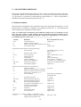
Table 2: Requirements for all commands that can be repeated in a main input file.
Label
trip
trip
trip
trip
trip
trip
trip
trip
trip
Must be
repeated?
Yes
Yes
No
No
No
No
No
Maybe1
Maybe1
species
species
No
Yes
No sub-populations
@vulnerability
trip & species
@vertical_availability
trip & species
@areal_availability
trip & species
@population_area,
trip & species
@area_fished
trip & species
@lw_coeff
species3 or trip & species
No
No
No
No
Yes
No2
All = 1
All = 1
All = 1
All = stratum area
Command
@species
@preferences
@where
@change_strata
@reassign_strata
@new_strata
@change_stratum_area
@constant_speed
@constant_doorspread
@sub_populations
@phase_2
1
Default action if
command not repeated
Use default selects
No changes
No changes
No new strata
No changes
Depends on @preferences; 2Only needed for trip-species combinations where length-weight
coefficients are required (see Section 5.1.6); 3Use species label when the same coefficients are to be
used for all trips.
31
3.2 Other input files
All input files other than the main one (see Section 3.1) are flat files. That is, files containing
columns of data, with the column names in the first line. Columns should be separated by
white space (i.e., spaces or tabs) and the order of the columns doesn’t matter. Missing values
should be entered as NULL. The user specifies which flat files (if any) SurvCalc should read
using the run-time arguments -S , -T, -U, -V, -W, or -X (see Section 2). Each row of the flat
file corresponds to: a stratum (with -S); or a station (with -T or -X); or a catch record (i.e., for
each station there must be a row for each species caught at that station) (with –U); or a
subcatch record (i.e., for each station there must be a row for each subcatch of species caught
at that station) (with –W); or a length record (i.e., for each station, species, and subcatch,
there must be a row for each length that occurs in the LF in that subcatch of that species at
that station) (with –V).
The columns, and column names, required for the stratum (-S), catch (-U), subcatch file (-W),
and length (-V) files are precisely those given in Table 1. For the station file (-T), the only
obligatory columns are station_no and stratum (and trip_code if there is more than one trip).
Which of the other columns from this table are required depends on command
@preferences (e.g., column dist_doors is not needed if preferences.width_swept
is constant_doorspread).
For the station-catch file (-X), the only obligatory columns are station_no, stratum, and a fish
density with a label like XYZ_kg_km2, where XYZ is a user-specified species code (which
need not be an official species code). There can be densities for more than one species (e.g.,
HOK_kg_km2, HAK_kg_km2). The only other optional column is trip_code (a userprovided code, which need not be an official trip code), which is required only if the user
wishes to analyse more than one survey. Note that vulnerabilities and vertical availabilities
can not be entered as columns in this file. When a station-catch file is used it is assumed that
the fish density columns are already adjusted for vulnerability and vertical availability.
32
4. OUTPUT FILES
Most output from SurvCalc goes to the main output file (Section 4.1), which is named in the
command line (e.g., myfile in the example command line at the beginning of Section 2). If
requested, additional output goes to one or more flat files (Section 4.2) or a catch-at-age data
file (Section 4.3). The precision of many numbers in the output files, as specified by
command @output_precision, is discussed in Section 4.4.
4.1 Main output file
The structure of this file is most simply illustrated by the following, which shows the
structure of the main output file expected when the input file is as in the last example in
Section 3.1.6 and the task is calc_biomass, calc_biomass_and_LFs, or calc_LFs
(the indenting in what follows is simply used to illustrate the structure of the file; it does not
occur in the actual file).
Header
SELECTIONS for trip tan0617:
PREFERENCES for trip tan0617:
Results for species HOK in trip tan0617
Results for species HAK in trip tan0617
Results for species LIN in trip tan0617
Tables for trip tan0617
SELECTIONS for trip tan0714:
PREFERENCES for trip tan0714:
Results for species HOK in trip tan0714
Results for species HAK in trip tan0714
Tables for trip tan0714
For tasks output_flat_files and output_for_catch_at_age the main output
file contains only the header. For task output_LW_coeffs, it contains the header plus a
table of length-weight coefficients.
The header contains general information about the particular run of SurvCalc, including the
command line, the date, the version of SurvCalc (this is useful if bugs are subsequently found
in the program), the user name, and, if the survey data have been extracted from a database,
the SQLs that were used to do this. If LFs are calculated then the last line in the header
describes the LF scaling.
The SELECTIONS section contains two lists: one of the selected strata (including their
effective areas) and one of the selected stations (including the stratum associated with each).
The PREFERENCES is simply a repeat of the information in command @preferences.
The results for a particular species and trip always starts with a list of exclusions (which
stations and strata are excluded, and why) and summaries of the numbers of stations and
strata that were selected and used. After this, the remaining output is in a series of tables,
some obligatory and others optional, the latter being requested with command
@output_tables.
33
4.1.1
Tables in the main output file
area_swept_factors
width_swept_m
distance_towed_km
Obligatory table when area swept is calculated; produced for
each species-trip combination. Summary statistics for the
two factors that define area swept.
mean
min
120.56 104
5.47
3.82
stratum_summary
stratum
0001
0002
...
max
129.7
5.76
Obligatory table when biomasses are being calculated;
produced for each species-trip combination. One line per
stratum and including mean fish densities, biomass and c.v.
NtowsHOK is the number of tows with non-zero catch for
HOK (or whatever the specified species is). The area is the
population area, as′ (which may differ from the stratum area
if
commands
@areal_availability
or
@population_area are used).
area Ntows NtowsHOK kg/km2 biomass cv.biomass
2150
4
3
9
19
71
1318
4
4
24
31
48
biomass
Obligatory table when biomasses are being calculated;
produced for each species-trip combination. One line (the
first, with label all) for the total biomass, and then one line
for each requested sub-population, with user-supplied labels.
Lower and upper bounds are estimate +/– 2 s.e.s.
population
all
to60
60+
...
lbound biomass
31601
46081
-114
846
11830
20001
sub_biomass_by stratum
ubound
60561
1807
28172
cv Nstations
16
97
57
90
20
90
Optional table produced for each species-trip combination.
Contains biomass estimates, and c.v.s, for a single species by
sub-population and stratum; the column labels are usersupplied for each sub-population.
stratum to60 cv_to60 60+ cv_60+
0001
726
66 639
85
0004
87
71 3345
50
...
biomass_by_species
species
HOK
HAK
...
lbound biomass
31601
46081
1827
2628
Optional table produced for every trip in which more than
one species is analysed. Like the biomass table above,
containing one line (total biomass) per species.
ubound cv Nstations
60561 16
97
3429 15
97
34
biomass_by_species_stratum
stratum HOK cv_HOK
0001
1365
74
0002
206
35
...
biomass_by_species_trip
Optional table produced for every trip in which more than
one species is analysed. One line per stratum, containing
biomass estimates, and c.v.s, for all species analysed for that
trip.
HAK cv_HAK
19
71
31
48
Optional table, presented at the end of the output from a
multi-trip analysis, containing all biomass estimates,
including those for sub-populations (but not stratum
biomasses). This table is simply the union of all the biomass
tables, ordered by species, and then by trip within species.
species
trip population
HOK
tan0601
all
HOK
tan0601
to60
HOK
tan0601
60+
HOK
tan0701
all
...
projected_cvs
lbound biomass
31601
46081
-114
846
11830
20001
29701
51315
ubound
60561
1807
28172
63517
cv Nstations
16
97
57
90
20
90
18
95
Obligatory table when biomasses are calculated and
command @projected_cvs is used. Includes projected
c.v.s for all total biomasses (including sub-populations, if
any).
species population projected_cv
HOK
all
10
HOK
to60
23
HOK
60+
11
HAK
all
16
LF_correction_factors
Obligatory table for task calc_biomass_and_LFs;
produced for each species-trip combination (see CFs and CF
in Section 5.4).
stratum correction_factor
0001
1.08
0002
1.08
...
all
1.04
LF_overall
L
32
33
...
Nfemale
1
8
LFs_by_stratum
Obligatory table when LFs are calculated; produced for each
species-trip combination. A single table for the whole
population as follows (N means number measured; SN
means scaled number).
Nmale
3
5
Nunsexed
0
0
Nall
4
13
SNfemale
2199.1
9259.1
SNmale SNunsexed
1783.3
0
16399.2
0
SNall
3983.2
25658.3
Optional table; produced for each species-trip combination.
Same format as LF_overall, but with an additional initial
column, stratum.
35
LFs_by_station
Optional table; produced for each species-trip combination.
Same format as LF_overall, but with an additional initial
columns, stratum and station.
Number_measured
Optional table; produced for each species-trip combination.
One line per stratum (and a final summary line) containing
the number of fish measured by sex and stratum.
stratum
0001
0002
...
All
Nfemale
624
302
Nmale Nunsexed
656
1
131
0
2501
LF_totals
1765
Nall
1281
433
9
4275
Optional table; produced for each species-trip combination.
One line per stratum (and a final summary line) containing
LF totals, and their c.v.s, by stratum and sex
stratum SNfemale
SNmale SNunsexed
SNall cv_female cv_male cv_unsexed cv_all
0001
1163734.1 1463051.0
5269.5 2632054.6
39
44
100
35
0002
161545.6
69949.2
0 231494.9
17
8
0
36
...
All
7732192.2 5210113.8 39712.7 12982019.0
12
18
70
12
gains
Obligatory table for task phase_2_calc; produced for
each species. One line per stratum, number of column
determined by subcommand n_stations.
stratum
0001
0002
...
1
16.8
8.5
2
11.2
4.3
3
8
2.6
4
6
1.7
5
4.7
1.2
6
3.7
0.9
7
3.1
0.7
8
2.5
0.6
9
2.2
0.5
10
1.8
0.4
4.2 Output to flat files
Flat files contain columns of data, with the column names in the first line. Each row of the
flat file corresponds to: a stratum (with -s or -y); or a station (with -t or -w); or a catch record
(with -u); or a subcatch record (with -w); or a length record (with –v).
For -s, -t, -u, -v, or -w the columns are the same as those extracted from the corresponding
table in the database (see Section 3.1.1), or as provided by the user (with -S,-T,-U, -V, or -W).
4.2.1
Station-catch file
A file of station-catch data is output with –x switch in the command line if run time task is
one
of
output_flat_files,
calc_biomass,
calc_LFs,
or
calc_biomass_and_LFs.
The file contains all the columns names in the station table plus three columns for each of the
species analysed, as well as two columns for each of the sub_populations defined by the user.
For species XYZ, these columns are XYZ_kg (the catch weight, Ci), XYZ_kg_km (the linear
density, LDi), and XYZ_kg_km2 (the areal density, ADi). For sub_population ABC of
species XYZ, the two columns are XYZ_ABC_kg (the catch weight, ci), and
XYZ_ABC_kg_km2 (the areal density, adi). For stations from trips in which species XYZ is
not analyzed NULL is entered for all columns associated with this species.
36
4.2.2
Output to stratum-catch file
A file of stratum-catch data is output with -y switch in the command line if run time task is
one
of
output_flat_files,
calc_biomass,
calc_LFs,
or
calc_biomass_and_LFs.
The file contains columns trip_code, stratum, and area_km2 plus three columns for each of
the species analysed. For species XYZ, these columns are XYZ_kg (stratum mean catch
weight, (ΣiCi)/ns), XYZ_kg_km (the linear density, LDs), and XYZ_kg_km2 (the areal
density, ADs). For strata from trips in which species XYZ is not analyzed NULL is entered
for all columns associated with this species.
4.3 Catch-at-age data output
The command ‘SurvCalc –c > myout’ run produces, for every combination of trip and species
in the input file, a file that can be read by the catch-at-age function import.length.data, as well
as a ‘main output file’ (‘myout’ in the above example), whose format is described in Section
4.1. The catch-at-age files are either in the ‘survey’ or ‘survey.sub’ format, with the latter
format being used if there are any subcatches for the given trip and species.
The names of the catch-at-age files are not specified by the user. They are constructed from
the species and trip names in the form LFttttttccc.i (for format ‘survey’) or LFttttttcccsub.i
(for format ‘survey.sub’), where tttttt is the trip code, ccc is the species code, and i is an index
used by SurvCalc to ensure that any existing files don’t get overwritten. For example, the
first time you do a ‘SurvCalc –c’ run for HAK in trip tan0901 SurvCalc will produce the
output file LFtan0901HOK.1 (or LFtan0901HOKsub.1 if there were any subcatches). If you
then do another ‘SurvCalc –c’ run for the same species and trip, in the same directory without
deleting the first output file, then the new output file will be LFtan0901HOK.2 (or
LFtan0901HOKsub.2).
The ‘survey’ format is as follows:
comment line
trip
number_of_strata
length-weight parameters: male_a male_b female_a female_b {optionally
unsexed_a unsexed_b}
one row for each stratum: stratum_name stratum_area n_tows
and then a table of length records, with a header row as follows:
stratum, tow, kg/km2, length, no_m, no_f, no_t
and a whole bunch of data rows.
The ‘survey.sub’ format is the same as this except that the final table of length records has
header row
stratum, tow, subsample, kg/km2, subsample_kg/km2 length,
no_m, no_f, no_t
and two additional columns (‘subsample’ = subcatch number, and ‘subsample_kg/km2’).
37
4.4 Precision of numbers in output files
The degree of precision (expressed as a number of significant figures or decimal places) for
each of five types of output quantities is controlled by command @output_precision
(Table 3). The default levels for each output type were set on the basis that c.v.s are unlikely
to fall below 1% (and are usually much higher). Note that negative numbers can be used for
decimal places (e.g., 12345.67 presented to -2 decimal places is 12300).
Table 3:
Description of the quantities whose precision is controlled by command
@output_precision and the default level of precision (a number of either significant figures or
decimal places) assigned to each.
Quantity
density
Default
precision
4 sig. figs
biomass
4 sig. figs
LF_number
4 sig. figs
cv
gain
1 dec. place
0 dec. place
Description
all columns of type XYZ_kg, XYZ_kg/km, or XYZ_kg/km2 in
station-data and stratum-data output files
column kg/km2 in stratum_summary table
column kg/km2 in catch-at-age output
all biomasses (including lower and upper bounds) in tables
stratum_summary,
biomass,
sub_biomass_by_stratum,
biomass_by_species, and biomass_by_species_stratum
all scaled numbers in LF tables (i.e., all columns whose labels start with
‘SN’)
all columns in biomass or LF tables whose labels start with ‘cv’
all numbers in gain tables (described in Section 4.1.1)
38
5. CALCULATIONS IN SURVCALC
This section contains detailed descriptions of the six types of calculation made by SurvCalc:
of densities (Section 5.2), biomasses (Section 5.3), LFs (Section 5.4), phase-2 gain (Section
5.5), projected c.v.s (Section 5.6) and catch-at-age data (Section 5.7). These are preceded by
definitions of the data and notation used (Section 5.1).
5.1 Data and notation
The data used in calculations come from three sources: the main input file (Section 3.1); flat
files (Section 3.2); and the trawl database (see beginning of Section 3.1.1). The notation used
in the calculations is explained in Tables 4 and 5.
Table 4: Variables used in calculations, their definitions, and how they are calculated or where
they come from. Where a second variable is given in parentheses, the first variable is for the
whole population and the second is the analogous variable for a sub-population. See Section 5.7
for additional notation used for task output_for_catch_at_age.
Variable
B (b)
n
m
CF
Definition
How calculated/where from
overall biomass (t)
equation (7)
number of strata in survey
number of strata with LF samples or zero catch
LF correction factor
equation (24)
i indexes the selected stations for the specified trip:
time towed (h)
ti
di
Ci (ci)
wi
vi
uvi
fi
ADi (adi)
LDi
distance towed (n.mile)
catch weight (kg)
width of tow (m)
vulnerability
vertical availability
effective area fished (m2)
areal density (kg.km-2)
linear density (kg.km-1)
s indexes the selected strata for the specified trip:
as
stratum area (km2)
ns
number of selected stations in stratum s
ms
number of selected stations in stratum s
where there is LF data or Ci = 0
uas
areal availability
as′
ADs (ads)
LDs
ADs,LF
ps
Bs (bs)
CFs
Ks
population area (km2)
mean areal density (kg.km-2)
mean linear density (kg.km-1)
mean areal density (kg.km-2)
over stations with LF data or Ci = 0
proportion of catch taken
in stations with LF data
biomass (t)
LF correction factor
LF scaling factor
k indexes sex (1 = male, 2 = female, 3 = unsexed, 4 = all):
length-weight coefficients (calculates
a k, b k, c k
weight in g from length in cm
39
calculated from time_s, time_f,
date_s, date_f
Table 6
Table 6 (equations (10, 11))
Table 6
from @vulnerability
from @vertical_availability
fi = 1852diwiviuvi or @area_fished
equation (1) or station-data file
equation (2)
area_km2
from @areal_availability or
stratum-data file
as′ = as uas
equation (3)
equation (4)
equation (19)
equation (10)
equation (6)
equation (21)
equation (18)
from @lw_coeff
Table 4 continued:
j indexes the records in table t_lgth for station i and the specified trip and species (so the following
variables are derived from attributes in this table)
Variable
Definition
How calculated/where from
pij
proportion sampled
percent_samp/100
Nijk
number of fish by sex
no_m (k=1), no_f (k=2),
no_a–no_m–no_f (k=3), no_a (k=4)
Lij
length of fish (cm)
lgth
Wijk
bk + ck ln Lij
weight of fish (g)
Wijk = ak Lij
weight of fish of length l and sex k (g)
Wlk = ak l
l indexes fish length
Wlk
bk + ck ln l
SN refers to scaled numbers of fish; MSN is the mean scaled numbers; SN ′ is scaled numbers corrected
for consistency with biomass estimates and length-weight relationships
SNilk
of length l and sex k at station i
equation (13)
′
SNslk MSNslk SN slk of length l and sex k in stratum s
equations (14 or 16, 17, and 20)
SNlk SN lk′
of length l and sex k
equation (22, 23)
TN refers to total numbers (i.e., LF totals), which are sums over length of scaled numbers
TN ik = l SNilk
TNik
for station i
∑
∑ SN ′
TN sk′
for stratum s
TN sk′ =
MTNsk
for stratum s
MTN sk =
TN k′
Table 5: Conventions used in summations.
for task output_for_catch_at_age.
Symbol
∑
∑
∑
∑
∑
∑
∑
∑
∑
∑
TN k′ =
for the whole population
i
i ,LF
the ms stations in stratum s in which lengths were measured
s
s ,LF
jk
jk ,sub
(& equation (28))
∑ MSN
l
slk
=
∑
i , LF
TN ik
ms
∑ SN ′
l
lk
See Section 5.7 for a further convention used only
Range of summation
the ns stations in stratum s
i ,LF2
slk
l
stations in which either some lengths were measured or total catch was zero
the n strata in the survey
the strata in which some lengths were measured
all length records (j) and all sexes (k) for station i
values of j and k such that, for station i, the length Lij and the sex k are
within the required sub-population
j ,l
l
l ,sex
values of j such that, for station i, the length Lij = l
all lengths, l, measured at station i
EITHER all lengths, l, for k=4, if a single set of length-weight coefficients is provided
OR all lengths for k = 1,2,3, if length-weight coefficients are provided by sex
40
5.1.1
Note on subcatches
The notation (Nijk, Lij) and formulae (see below) used here for data from the table t_lgth are a
bit more complicated than those of Vignaux (1994) because they allow for the possibility of
what are called (in database trawl) subcatches, which is to say more than one length sample
for a given species from a given station (e.g., one species in a catch may be divided roughly
into two parts, ‘small fish’ and ‘others’, with each part being weighed separately, and having
its own random length sample). This means that there may be two (or more) records in t_lgth
with the same values of trip_code, station_no, species, and lgth. The sum ∑ j ,l , used in
calculating an LF for each tow (see below), combines such records.
In trawlsurvey, this summation is not done, and this produces anomalies in the output station
LFs, as shown in the following example, in which there are two lines for fish of length 42 cm
in station 79. However, this error affects only the station LFs; the stratum and overall LFs
are OK.
stn
...
79
79
79
79
...
str
0017
0017
0017
0017
5.1.2
L Nall Nmale Nfemale Nunsexed
41
42
42
43
12
9
1
11
8
3
1
8
4
6
0
3
SNall SNmale SNfemale SNunsexed
0 338.11 225.41
0 253.58 84.53
0 14.77 14.77
0 309.94 225.41
112.70
169.06
0.00
84.53
0
0
0
0
Note on stations and strata without LF data
There can be two types of stations (or strata) without LF data: A, those with no catch of the
target species, and B, those with a non-zero catch from which no fish were measured. It is
important to notice that both types are excluded from the summations ∑ i ,LF (for stations)
and
∑
s ,LF
(for strata), but that only type B is excluded in defining the variables ms and m
and in the summation
5.1.3
∑
i ,LF2
.
Excluding stations and strata
For tasks calc_biomass, calc_LFs, calc_biomass_and_LFs, and phase_2_calc,
SurvCalc sometimes excludes some stations and/or strata because of inadequate data.
A station is excluded if A, it is not possible to calculate the fish density, ADi, because of
missing data (e.g., distance towed or width of tow missing, with no default provided) or B, the
stratum it is in is excluded. Note that criterion A does not apply when the task is calc_LFs
and @LF_scaling is not numbers_per_km2 (because fish densities are not calculated in
this case).
The criterion for excluding a stratum depends on the task. Stratum s is excluded if ns < 2 for
tasks calc_biomass and phase_2_calc, or if ms < 2 for task calc_biomass_and_LFs.
When sub-population biomasses are calculated then any stratum in which ps < 0.3 is excluded
(but only for these biomasses) (see Section 5.3.1).
41
5.1.4
User preferences for fish-density variables
When command @preferences is used (see Section 3.1.4) it specifies the user’s
preferences for the variables di, wi, and Ci. For each variable and station, the option used will
depend on what data are available. The first option should be used unless the required data
are not available, in which case the second option is used, unless the required data are not
available, etc. All stations for which it is not possible to calculate all three variables (di, wi,
Ci) are dropped from the analysis (and an appropriate error message is included in the main
output file). The options for each variable, and the associated values, are given in Table 6.
Table 6: Three variable with user-supplied calculation options, the associated sub-command of
@preferences, and the value of the variable according to the option used.
Variable Sub-Command
distance_towed
di
Option
recorded_distance
from_lat_lon
from_recorded_speed
from_constant_speed
Value
distance in t_station
calculated from following attributes in
t_station: lat_s, NorS_s, long_s,
EorW_s, lat_f, NorS_f, long_f, EorW_f
speed in t_station x ti
@constant_speed x ti
wi
width_swept
recorded_doorspread
constant_doorspread
recorded_wingspread
dist_doors in t_station
@constant_doorspread
dist_wings in t_station
Ci
catch_weight
recorded
weight1 in t_catch
Ci = 0.001∑ jk NijkWijk pij
calculated
1
Note that if there is no record in t_catch for the given species, station, and trip this means that Ci = 0.
5.1.5
Calculation of c.v.s
All c.v.s are calculated and presented as percentages. Unless otherwise stated, the c.v. of any
variable, X, is calculated as c.v.(X) = 100s.e.(X)/X.
5.1.6
Use of length-weight coefficients
Length-weight coefficients, ak, bk, ck, are not always required. They are used only in three
situations:
– when Ci is calculated, rather than being a recorded value (Table 6),
– when sub-population biomasses are calculated (see equation (11), Section 5.3.1), and
– when LFs are calculated and scaled to numbers in population (see calculation of CFs
and CF in Section 5.4).
42
5.2 Calculating fish densities
One or both of two types of densities may be calculated: areal (kg/km2) or linear (kg/km).
The former are always used for calculating either biomass or gains. The latter (not defined if
@survey_type is pot) are calculated only if requested (with commands
@station_data_columns and/or @stratum_data_columns) as output columns in
station or stratum tables.
When a station-catch input file is used (see Section 3.2) the station densities are read directly
from this file: ADi from columns with names like XYZ_kg_km2; LDi from columns with
names like XYZ_kg_km. Otherwise, they are calculated as
ADi = 106 Ci fi
(1)
LDi = 1000Ci (1.852di uvi vi )
Stratum mean densities are calculated as
( ∑ AD )
= ( ∑ LD )
(2)
ADs =
i
i
ns
(3)
LDs
i
i
ns
(4)
The s.e.s of areal densities are given by
(
2
s.e. ( ADs ) =  ∑ i ( ADi − ADs ) 
[n ( n
s
s
− 1)]
)
0.5
(5)
5.3 Calculating biomasses
Stratum and overall biomasses are calculated as
Bs = ADs as′ 1000
(6)
B = ∑s Bs
(7)
and their standard errors are calculated as
s.e. ( Bs ) = s.e. ( ADs ) as′ 1000
s.e. ( B ) = 
∑ s
5.3.1
2 0.5
s.e. ( Bs ) 

(8)
(9)
Calculating sub-population biomasses
The first step in calculating sub-population biomasses for each stratum is the calculation of
sub-population catches, ci, for each station.
In the special case of a stratum with zero catch (i.e., ΣiCi = 0), the sub-population catch is set
to 0 for all stations in that stratum.
For all other strata, a check is done to see whether there are enough LF data to warrant the
calculation of sub-population catches. This involves the calculation of the quantity
43
ps = ∑ i ,LF Ci
∑C
i
i
(10)
which is the proportion of the catch in stratum s that is from stations with LF data. Subpopulation biomass estimates will be unreliable in strata where ps is low. Any strata with
ps < 0.3 are dropped from the calculation of sub-population biomasses and a warning message
is included in the output file. Strata with 0.3 ≤ ps < 0.5 are included in the calculation of subpopulation biomasses but a warning message is printed.
Where ps ≥ 0.3, the sub-population catch for station i is estimated as
ci = Ci

∑
NijkWijk pij   ∑ jk NijkWijk pij 
 

jk ,sub
(11)
for each station with LF data, and
ci = Ci  ∑ i′,LF adi ′   ∑ i ′,LF ADi ′ 
(12)
for stations without such data.
The remaining calculations (of densities, adi and ads, biomasses, bs and b, and s.e.s, for ads, bs
and b) use the same equations as for population biomass (i.e., equations 1, 3, and 5-9) except
that each population variable is replaced by its sub-population analogue (as defined in Table
4).
5.4 Calculating LFs
The equation for calculating SNilk, the scaled LF for the ith tow, depends on which option has
been selected with command @LF_scaling:
unscaled

∑ j ,l Nijk

 1000∑ j ,l ( N ijk pij )
numbers_per_1000

 ∑ l ′  ∑ j ,l ′ ( N ijk pij ) 
SN ilk = 
numbers_per_tow
∑ j ,l ( Nijk pij )

 ∑ ( N ijk ( pij ti ) )
numbers_per_hour
j ,l


numbers_per_km2 or
6
∑ j ,l (10 N ijk ( pij fi ) ) numbers_in_population
(13)
For stations with zero catches, SNilk = 0 for all l and k.
How the stratum and overall LFs are calculated depends on the task. If it is calc_LFs these
are simple (i.e., unweighted) sums or averages, with no correction for stations or strata
without LFs:
∑ SN
( ∑ SN )

SN slk = 
i ,LF
for unscaled LFs
ilk
i ,LF
ilk
(14)
ms
44
otherwise
∑
( ∑

SN lk = 
s ,LF
SN slk
)
SN slk
s ,LF
for unscaled LFs
(15)
m
otherwise
These equations differ from those in trawlsurvey, where SNslk and SNlk are always calculated
as sums for a calc_LFs analysis. That is, SN slk = i ,LF SNilk and SNlk = s ,LF SN slk .
∑
∑
When the task is calc_biomass_and_LFs the stratum LFs are calculated by averaging
the station LFs, scaling using the population area, and then adjusting for strata with no LF
data
SN slk = MSN slk K s
(∑
MSN slk =
where
Ks =
ADs ,LF =
and
i ,LF
SNilk
as′ ADs
ADs ,LF
(∑
i ,LF
ADi
(16)
)
ms
(17)
(18)
)
ms
(19)
They are then corrected so that the estimated numbers of fish are consistent with the estimated
biomass and length-weight relationships
′ = SN slk CFs
SN slk
CFs = 106 Bs
where
∑
l ,sex
(20)
SN slkWlk
(21)
Overall LFs are calculated using
SN lk =
∑
s ,LF
SN slk
B
∑
B
s ,LF s
(22)
(note that for surveys in which there are LF data in all strata this equation becomes a simple
sum, SNlk =
∑ SN
s
slk
) and then corrected for consistency with the estimated biomass and
length-weight relationships
SNlk′ = SNlk CF
where
5.4.1
CF = 10 B
6
∑
l ,sex
SNlkWlk
(23)
(24)
Calculating c.v.s for LFs
C.v.s for LFs are calculated only when the task is calc_biomass_and_LFs, and then
only for corrected LF totals, TN sk′ (for each stratum) and TN k′ (for the whole population),
using the equations
c. v. ( TN sk′ ) = 100s.e. ( MTN sk ) MTN sk
45
(25)
c . v . ( TN k′ ) =
and
100
(∑
s .e . ( MTN sk ) K s2
s ,LF
2
∑
)
MTN sk K s
s ,LF
 ∑ i ,LF2 ( TN ik − MTN sk ) 2 

s .e. ( MTN sk ) = 


ms ( ms − 1)


where
0.5
(26)
0.5
(27)
The derivation of equations (26-27) is worth explaining. These c.v.s take into account only
the uncertainty arising from the variation in numbers between stations in the same stratum.
All other sources of uncertainty are ignored. Thus, because we can write
TN sk′ = MTN sk K s CFs
(28)
and we ignore uncertainty in Ks and CFs, c. v. ( TN sk′ ) = c. v. ( MTN sk ) , which leads to
equation (25). Similarly, we can write
TN k′ =
(∑
)

MTN sk K s 
s ,LF
B
 ∑ s ,LF Bs

CF 

but we ignore uncertainty in both the Ks and the term in square brackets.
c.v. ( TNk′ ) = c.v.
(∑
s ,LF
)
(29)
Thus
MTNsk Ks , which leads to equation (26).
5.5 Calculating phase-2 gains
Gains are calculated only when the task is phase_2_calc, and the calculations are based
on the equations in Francis (1984). When these calculations are done, it is assumed that the
selected stations (i.e., those defined by commands in Section 3.1.1, or included in the station
flat file, if there is one) are all the phase-1 stations in a 2-phase survey. Sometimes, for
logistical reasons, the calculations will be done before all phase-1 stations are completed
and/or after some phase-2 stations have been done. In this situation, the calculations should
use all completed phase-1 stations but not any of the phase-2 stations (to use phase-2 stations
in the calculations would effectively change the survey from 2-phase to multi-phase, and the
statistical behaviour of multi-phase surveys of this type are not known).
A table of gains will be calculated for each species in phase_2.species. If subpopulations are defined for any of these species, then an additional table of gains will be
calculated for each sub-population.
Each table of gains will have n rows (i.e., one per stratum) and phase_2.n_station
columns. Let Gse be the relative gain (i.e., the estimated reduction in the biomass variance)
associated with adding the eth extra station to the sth stratum. To calculate Gse, we need first
to calculate ADs (and ads if sub-populations are involved) and its s.e. (using equations 1, 3,
and 5).
The formula for Gse depends on whether phase_2.algorithm is
mean_squared or variance:
46

( as′ ADs )2

 ( ns + e − 1)( ns + e )
Gse = 
2
 ( as′ s.e. ( ADs ) ) ns
 ( n + e − 1)( n + e )
 s
s
mean_squared
(30)
variance
(for sub-populations, replace ADs by ads in this equation).
Before being output, each table of gains is to have maximum value 100 using the equation
Gse = 100Gse max s ( Gs1 )
(31)
5.6 Calculating projected c.v.s
Projected c.v.s are calculated for all biomasses (including those for sub-populations) when the
task is calc_biomass or calc_biomass_and_LFs and there is a @projected_cvs
command block (see Section 3.1.4) in the main input file. In these calculations, ns is the
number of stations already completed in stratum s, and es is the number of stations yet to be
completed (the latter being specified in the @projected_cvs command block). For the
projections it is assumed that, in each stratum, the mean and variance of the catch rates for the
remaining stations will be exactly the same as for the existing stations.
The calculations use the same equations as are used in the calculation of the usual biomass
c.v.s (i.e., equations (8) and (9)) except that, for strata that are not yet completed (i.e., those
specified in the @projected_cvs command block), s.e.(ADs) (or s.e.(ads) in the case of
sub-populations) in equation (8) is replaced by s.e.proj(ADs) (or s.e.proj(ads)) where these are
defined by
s.e.proj ( ADs ) = s.e. ( ADs ) ( ns
and
s.e.proj ( ad s ) = s.e. ( ad s ) ( ns
47
( ns + es ) )
( ns + es ) )
0.5
0.5
(32)
(33)
5.7 Output for catch-at-age
With task output_for_catch_at_age SurvCalc must read additional material from the
database (beyond what is given in Table 1) and may have to do some additional calculations.
The first additional material that must be read from the database is column subcatch_no,
from database table lgth. If this column is always equal to 1 there are no subcatches, so the
output will be in format ‘survey’ and no additional calculations are required. The column
kg/km2 in the output file (see Section 4.3) will contain ADi.
If there are any subcatches, the output will be in format ‘survey.sub’, column subsample
in the output file will be subcatch_no from table lgth, and column subsample_kg/km2
will contain the subcatch catch rate ADic, where c indexes the subcatches (for the species in
6
question) at station i, and ADic = 10 Cic fi .
Where Cic comes from depends on what option is being used for catch_weight (as specified in
the @preferences command – see Section 3.1.4). With option recorded, Cic is taken
directly from column weight in table t_subcatch (so SurvCalc must read columns trip_code,
station_no, species, subcatch_no, and weight from this table). With option calculated,
Cic = 0.001∑ jk ,c NijkWijk pij , where ∑ jk ,c means the sum over all sexes (k) and all length
records (j) in station i for which subcatch_no = c.
48
6. SurvCalc AND 2-PHASE SURVEYS
SurvCalc, and the associated R library, can be used in three ways to help in 2-phase surveys.
First, the R function allocate can be used in designing the survey (see Appendix 2). One
aspect of the design is the percentage of stations to be done in phase 1 of the survey. Note
that although Francis (1984) recommended this be 75%, the current recommendation, based
on much more extensive simulations, is 90% (Francis 2006).
Second, task phase2_calc of SurvCalc can be used at the end of phase 1 to help in
determining the allocation of phase-2 stations to strata. For example, suppose our target
species is hoki and, at the end of phase 1, we decide there is sufficient remaining survey time
to complete six phase-2 stations. Then we could insert the command block
@phase_2 HOK
n_stations 6
into our main input file, and run SurvCalc -2 > myfile.
Within the output file, myfile, there will be a table of gains for hoki which might look like
stratum
0001
0002
0003
0004
0005
1
19
62
100
96
43
2
15
44
60
64
32
3
12
33
40
46
25
4
10
26
29
34
20
5
8
21
21
27
16
6
7
17
17
21
14
In this example, the six biggest numbers in the table have been underlined to help illustrate
how the table of gains should be interpreted. This shows us that the optimum allocation for 6
phase-2 stations is one station in stratum 0002, two stations in stratum 0003, and 3 stations in
stratum 0004. If it turned out that there was time only for five phase-2 stations, then we
should ignore the smallest underlined number, and thus do only two extra stations in stratum
0003.
The third way that SurvCalc can be useful in 2-phase surveys is in evaluating alternative
phase-2 allocations using the command @projected_cvs. If, for example, hake was also
a target species in the above survey, we would need to add the command block
@phase_2 HAK
n_stations 6
to our main input file before running SurvCalc -2 > myfile. Then myfile would
contain two tables of gains (one for hoki, and one for hake), from which we could construct a
table like the following showing two alternative phase-2 allocations
stratum
0001
0002
0003
0004
0005
phase-2 allocation
for HOK
for HAK
0
2
1
2
2
1
3
1
0
0
So, which phase-2 allocation should we use: the one for hoki, the one for hake, or some
compromise between the two? To answer this question, the first thing to do is to find out
49
what c.v.s we might expect to get for the hoki and hake biomass estimates using each of the
above allocations. To evaluate the hoki allocation we would add the command block
@projected_cvs
strata
0002 0003 0004
extra_stations
1
2
3
and run SurvCalc -b > myfile. As well as calculating all the phase-1 biomass
estimates and c.v.s, this run will produce a table like
species population
HOK
all
HAK
all
…
projected_cv
18.3
25.7
giving estimates of the likely c.v.s at the end of the survey if we were to use the hoki
allocation. We can repeat this run, changing the allocation in the @projected_cvs
command block until, by trial and error, we find the most suitable phase-2 allocation.
Another reason for considering alternative phase-2 allocations is that some strata may be
more expensive (in terms of steaming time) to return to than others. Suppose, for example,
that in the above example stratum 0002 was so far away that including it in phase 2 would
mean that there was time for only five phase-2 stations.
Then we could use
@projected_cvs to compare the projected c.v.s from the following two alternative
allocations.
stratum
0001
0002
0003
0004
0005
Total
phase-2 allocation
with str 0002 without str 0002
0
0
1
0
2
2
2
3
0
1
5
6
The first of these allocations is what we get from the above table of gains if we allocate only
five phase-2 stations, and the second is the result of allocating six phase-2 stations but
ignoring stratum 0002.
Some practical considerations
In theory, the rule is that our phase-2 calculations (using either task phase2_calc, or task
calc_biomass with command @projected_cvs) should be done only after we have
finished all phase-1 stations, and before we have started phase 2. However, it is perfectly
acceptable to break this rule in some situations.
Remote strata provide a good reason to do phase-2 calculations before the end of phase 1.
After completing the phase-1 stations in a remote stratum we might want to use task
phase2_calc to work out, on the basis of the phase-1 stations completed to date, whether
we are likely to need any phase-2 stations in that stratum and, if so, approximately how many.
If it looks like some phase-2 stations will be needed in this stratum it is quite permissible to
do them immediately, before leaving the area.
50
Another reason to break the rule is if, part-way through phase 2, it becomes clear that the
actual number of phase-2 stations will differ from what was assumed, so that there is a need
to modify the original phase-2 allocation.
There is one rule about phase-2 calculations that should never be broken. That is, you must
never include catches from phase-2 stations when doing phase-2 calculations. Suppose, for
example, that during phase 1 you added two phase-2 stations (numbers, 32 and 33, say) in a
remote stratum. Then these stations must be excluded from any subsequent phase-2
calculations. This could be done using subcommand t_station station_no not in
(32,33) of command @where.
If you were already using this subcommand (say to
exclude stations with poor gear performance) then this restriction can be added as
t_station gear_perf < 3 and station_no not in (32,33) Similarly,
suppose you had completed 100 phase-1 stations (stations 1–100) and were part-way through
phase 2 when you wanted to repeat the phase-2 calculations. Then you could use
subcommand t_station station_no < 101 to exclude phase-2 stations from these
calculations.
7. REFERENCES
Bull, B.; Dunn, A. (2002). Catch-at-age user manual v1.06.2002/09/12. NIWA Internal
report 114. 23 p. (Unpublished report held in NIWA library, Wellington.)
Bull, B.; Francis, R.I.C.C.; Dunn, A.; McKenzie, A.; Gilbert, D.J.; Smith, M.H.; Bian, R.
(2008). CASAL (C++ algorithmic stock assessment laboratory): CASAL User
Manual v2.20-2008/02/14. NIWA Technical Report. 275 p.
Francis, R.I.C.C. (1984). An adaptive strategy for stratified random trawl surveys. New
Zealand Journal of Marine and Freshwater Research 18(1): 59-71.
Francis, R.I.C.C. (2006). Optimum allocation of stations to strata in trawl surveys. New
Zealand Fisheries Assessment Report 2006/23. 50 p.
Mackay, K.A. (2000). Database documentation: trawl. NIWA Internal report 73. 48 p.
(Unpblished report held in the NIWA library, Wellington. Latest electronic version
available
on
NIWA
intranet
at
http://seaspray.niwa.co.nz/stockmon/database%20documents)
Vignaux, M. (1994). Documentation of trawlsurvey analysis program. MAF Fisheries Greta
Point Internal Report 225. 44 p. (Unpublished report held in the NIWA library,
Wellington.)
51
8. APPENDIX 1: COMMAND BLOCK FORMAT
The main input file for SurvCalc uses a command-block format similar to that used in CASAL
(Bull et al. 2008). That is, this file consists of a series of command-blocks, which may occur
in any order. Each command-block either consists of a single command (starting with the
symbol @) and its arguments, or a command (starting with @) and an optional label and one
or more subcommands, i.e.,
@command arguments
or
@command [label]
[subcommand arguments]
[subcommand arguments]
[…]
Blank lines are ignored, as is extra white space between arguments. Comments beginning
with ‘#’ are ignored. If you want to remove a group of commands or subcommands using ‘#’,
then comment out the whole block, not just the first line. Alternatively, you can comment out
an entire block by placing curly brackets around the text that you want to comment out. Put in
a ‘{’ as the first character on the line to start the comment block, then end it with ‘}’. All lines
(including line breaks) between ‘{’ and ‘}’ inclusive are ignored. (These should ideally be the
first character on a line, but if not, then the entire line will be treated as part of the comment
block.)
Don’t put extra white space before a @ character (which must also be the first character on
the line). Make sure the file ends with a carriage return. Commands and subcommands must
consist of letters and/or underscores, and must not contain a full-point (‘.’).
There is no need to mark the end of a command block. This is automatically recognised by
either the end of the file or the start of the next command block, which is marked by the @ on
the first character of a line.
Also note that the commands, sub-commands, and arguments in the parameter files are case
sensitive.
Some commands can never have subcommands (such as @survey_type). If a command has
no subcommands, then it has to have arguments, which are placed on the same line as the
command. All other commands have no arguments, but have subcommands instead. Some
commands can be used multiple times and if they are they must have a different label each
time (see Table 2).
52
9. APPENDIX 2: THE SURVCALC R LIBRARY
This library can be downloaded from https://one.niwa.co.nz/display/FISHMOD/SurvCalc. It
contains two main functions: input.SurvCalc and allocate.
input.SurvCalc
Function input.SurvCalc simply reads the main output file of SurvCalc into R. Thus if
you have a SurvCalc output file myout in directory H:\proj\hok you can read this into the R
object hokout using the R command
hokout <- input.SurvCalc(‘H:/proj/hok/myout’)
or, alternatively
hokout <- input.SurvCalc(‘myout’,‘H:/proj/hok’)
The object hokout is a list of lists that is structured hierarchically, by trips and then species.
For example, all the output concerning trip buc8501 in myout is contained in the list
hokout$buc8501.
To
see
what
tables
are
there,
simply
type
names(hokout$buc8501), which may return something like
[1] "SELECTIONS"
"RUN PARAMETERS" "ORH" “OEO”
hokout$buc8501$SELECTIONS would contain information about the strata and stations
selected for this trip, and hokout$buc8501$"RUN PARAMETERS" would contain the
user-supplied preferences for distance towed, width swept, etc.
Similarly, typing names(hokout$buc8501$ORH) lists the output tables for ORH in trip
buc8501. For a description of all tables that can occur in a main output file from SurvCalc
see Section 4.1.
allocate
Function allocate is useful at the survey design phase. It uses historical data from
previous surveys in the same area to work out how many stations should be allocated to each
survey stratum. It can be used in two different ways, as illustrated by the following calls.
allocate(constraint=’cv’, limit=20, strata=mystrat, data=mydat)
allocate(constraint=’stations’, limit=20, strata=mystrat, data=mydat)
The first call calculates the minimum number of stations, and their allocation to strata, to
achieve a c.v. of 20%, whereas the second calculates the best allocation given that there will
be a total of 20 stations.
In both cases, mystrat should be a dataframe containing stratum information in the format
stratum
0001
0003
…
area
1245
347
minimum
3
3
maximum
20
15
53
with the last two columns specify the minimum and maximum number of stations allowed in
each stratum, and mydat should be a dataframe containing the historical data in the format
stratum survey
0001
tan0303
0001
tan0303
0001
tan0303
0002
tan0303
0002
tan0303
…
0001
tan0402
…
catch
3.7
2.5
12.1
4.2
2.8
5.3
where the last column contains catch rates (e.g., t km-1 or t km-2, etc).
The output from allocate is a list with three components: cv (the estimated c.v. achieved
by the calculated allocation); stations (the total number of stations); and allocation
(the allocation of those stations to the strata). For example, the output from the first call
above might look like the following
$cv
[1] 19.8
$stations
[1] 32
$allocation
stratum stations
1
0001
17
2
0002
12
3
0003
3
which would indicate that 32 stations (with 17, 12, and 3 in strata 0001, 0002, and 0003,
respectively) could be expected to achieve a c.v. of 19.8%.
It is not uncommon for surveys to have separate target c.v.s for two or more species. In this
case we would need to construct a different dataframe of historical catch rates for each
species, and run allocate with each of these in turn. In this case it is of interest to find out
what c.v. would be expected for one species if we used the optimal allocation for the other
species. This is easily done by modifying the strata dataframe so that for each stratum the
minimum and maximum numbers of stations are both set equal to the optimal number.
It’s important to understand that allocate is a very simple function, which makes no
allowance for the very real possibility that the distribution of fish in the survey being planned
may be quite different from that in the historical surveys. For this reason it is prudent to be
conservative in its use. For example, it is common to use allocate to determine a station
allocation that will achieve the target c.v.s in phase 1 of a 2-phase survey. Then, if fish
distributions during the survey differ substantially from those in previous surveys, so that the
target c.v.s are not met during phase 1, there is still a possibility that they will be met by the
end of phase 2.
54