1
APEX-MPI-MAN-0012
Atacama Pathfinder
EXperiment
Revision: 1.2.1
Release:
May 3, 2013
Category: 4
User Manual
Author:
H.Hafok
APEX Calibration and Data
Reduction Manual
Edward Polehampton,
Heiko Hafok
Keywords:
Calibration, APEX
Author Signature: H.Hafok
Date: May 3, 2013
Approved by: D.Muders
Signature:
Institute: MPIfR
Date:
Released by:
Signature:
Institute:
Date:
APEX
APEX Calibration and Data Reduction Manual
Change Record
Revision
Date
Author
0.0
0.1
0.2
0.3
1.0
1.1
1.2
1.2.1
2005-06-20
2005-09-14
2005-09-16
2009-02-02
2009-04-27
2010-03-08
2010-03-15
2013-05-03
E. Polehampton
E. Polehampton
E. Polehampton
H. Hafok
H. Hafok
H. Hafok
H. Hafok
D. Muders
Create Date: May 3, 2013
Section/
Page affected
All
All
All
All
All
All
All
Title
Page 2
Remarks
Initial Version
transfer to official format
minor updates, add script examples
revisited, including several changes
minor changes concerning the gain array , release version
added description of fsw modes
added preset of water
changed document category
Contact author: H.Hafok
APEX
APEX Calibration and Data Reduction Manual
Contents
1 Introduction
1.1
Calibrator aim . . .
1.2
Online case . . . . .
1.3
Offline . . . . . . . .
1.4
Internal data storage
.
.
.
.
.
.
.
.
.
.
.
.
.
.
.
.
4
4
4
5
6
.
.
.
.
.
.
.
.
.
.
.
.
.
.
.
.
.
.
.
.
.
.
.
.
.
.
.
.
.
.
.
.
.
.
.
.
.
.
.
.
.
.
.
.
.
.
.
.
.
.
.
.
.
.
.
.
.
.
.
.
.
.
.
.
.
.
.
.
.
.
.
.
.
.
.
.
.
.
.
.
.
.
.
.
.
.
.
.
.
.
.
.
.
.
.
.
.
.
.
.
.
.
.
.
.
.
.
.
.
.
.
.
.
.
.
.
.
.
.
.
.
.
.
.
.
.
.
.
.
.
.
.
2 Reduction of calibration observations
2.1
Calibration method . . . . . . .
2.2
Atmospheric model . . . . . . .
2.3
Channelwise calibration . . . .
2.4
Alternative calibration methods
2.5
Water vapour radiometer . . . .
.
.
.
.
.
.
.
.
.
.
.
.
.
.
.
.
.
.
.
.
.
.
.
.
.
.
.
.
.
.
.
.
.
.
.
.
.
.
.
.
.
.
.
.
.
.
.
.
.
.
.
.
.
.
.
.
.
.
.
.
.
.
.
.
.
.
.
.
.
.
.
.
.
.
.
.
.
.
.
.
.
.
.
.
.
.
.
.
.
.
.
.
.
.
.
.
.
.
.
.
.
.
.
.
.
.
.
.
.
.
.
.
.
.
.
.
.
.
.
.
.
.
.
.
.
.
.
.
.
.
.
.
.
.
.
.
.
.
.
.
.
.
.
.
.
.
.
.
.
.
.
.
.
.
.
7
. 7
. 9
. 10
. 10
. 11
3 Reduction of other heterodyne observing modes
3.1
Science data reduction . . . . . . . . . . .
3.2
Frequency Switch Observations . . . . . .
3.3
Position Calculation . . . . . . . . . . . .
3.4
Pointings . . . . . . . . . . . . . . . . . .
3.5
Focus . . . . . . . . . . . . . . . . . . . .
3.6
Skydip . . . . . . . . . . . . . . . . . . .
.
.
.
.
.
.
.
.
.
.
.
.
.
.
.
.
.
.
.
.
.
.
.
.
.
.
.
.
.
.
.
.
.
.
.
.
.
.
.
.
.
.
.
.
.
.
.
.
.
.
.
.
.
.
.
.
.
.
.
.
.
.
.
.
.
.
.
.
.
.
.
.
.
.
.
.
.
.
.
.
.
.
.
.
.
.
.
.
.
.
.
.
.
.
.
.
.
.
.
.
.
.
.
.
.
.
.
.
.
.
.
.
.
.
.
.
.
.
.
.
.
.
.
.
.
.
.
.
.
.
.
.
.
.
.
.
.
.
.
.
.
.
.
.
.
.
.
.
.
.
.
.
.
.
.
.
11
11
12
13
14
14
15
4 Offline Data Reduction
4.1
Basic functions . . . . . . . . . . . . . . . . . . . . . . . . .
4.1.1
help(methodName) . . . . . . . . . . . . . . . . . .
4.1.2
setInteractive(0|1) . . . . . . . . . . . . . . . .
4.1.3
setFitsDir(’directory’) . . . . . . . . . . . . .
4.1.4
setColdLoadParams(frontend, yfactor, tCold)
4.1.5
show and reset . . . . . . . . . . . . . . . . . . . .
4.1.6
reduce(ScanNum) . . . . . . . . . . . . . . . . . . .
4.2
Working with data entity objects . . . . . . . . . . . . . . . .
4.2.1
Displaying information: plotting and printing . . . .
4.2.2
Writing to CLASS . . . . . . . . . . . . . . . . . .
4.3
Further details for individual observing modes . . . . . . . . . .
4.3.1
Calibration . . . . . . . . . . . . . . . . . . . . . .
4.3.2
Pointing, focus, skydip . . . . . . . . . . . . . . . .
4.4
Reading a FITS file by hand . . . . . . . . . . . . . . . . . . .
4.5
Atmospheric model features . . . . . . . . . . . . . . . . . . .
4.5.1
plotATMspectrum . . . . . . . . . . . . . . . . . . .
.
.
.
.
.
.
.
.
.
.
.
.
.
.
.
.
.
.
.
.
.
.
.
.
.
.
.
.
.
.
.
.
.
.
.
.
.
.
.
.
.
.
.
.
.
.
.
.
.
.
.
.
.
.
.
.
.
.
.
.
.
.
.
.
.
.
.
.
.
.
.
.
.
.
.
.
.
.
.
.
.
.
.
.
.
.
.
.
.
.
.
.
.
.
.
.
.
.
.
.
.
.
.
.
.
.
.
.
.
.
.
.
.
.
.
.
.
.
.
.
.
.
.
.
.
.
.
.
.
.
.
.
.
.
.
.
.
.
.
.
.
.
.
.
.
.
.
.
.
.
.
.
.
.
.
.
.
.
.
.
.
.
.
.
.
.
.
.
.
.
.
.
.
.
.
.
.
.
.
.
.
.
.
.
.
.
.
.
.
.
.
.
.
.
.
.
.
.
.
.
.
.
.
.
.
.
.
.
.
.
.
.
.
.
.
.
.
.
.
.
.
.
.
.
.
.
.
.
.
.
.
.
.
.
.
.
.
.
.
.
17
17
17
17
17
17
17
18
18
18
20
20
20
21
22
23
23
Create Date: May 3, 2013
.
.
.
.
Page 3
Contact author: H.Hafok
APEX
1
APEX Calibration and Data Reduction Manual
Introduction
1.1
Calibrator aim
The APEX Calibrator is the online and offline reduction pipeline software for observations at the APEX
telescope. It will read raw data MBFITS files and reduce these depending on the content. It will analyse
automatically pointing, focus, skydip, calibration and astronomical observations in various modes for
heterodyne receivers and bolometers, taking proper care of different observing modes and scan types.
For spectral heterodyne obeservations the calibration pipeline will produce CLASS files containing
calibrated data. For Bolometer observations the APEX Calibrator will produce quicklook results by
using certain BoA routines. For the latter the results may differ compared to a precise interactive analysis.
For the online case the subscan number is also supplied, so that the reduction can proceed sequentially
for each subscan whilst the scan is observed. For offline processing more parameters can be specified to
further contrain the processing (e.g. FeBe, BaseBand1 ). Calibrations are stored internally in Python
dictionaries so that they can be applied tho the following scans. Pointing, focus, skydip and calibration
information is also stored and the latest value can be retrieved by the online system so that these can be
applied to the telescope.
All observing mode specific decisions and data storage that is independent of the frontend type (heterodyne
or bolometer) is taken care of within the CalibController module. Heterodyne and bolometer specific
reduction is then carried out by the HeterodyneReducer and BolometerReducer respectively. The
bolometer reduction makes use of the Bolometer Analysis (BoA) software. Heterodyne processing makes
use of the Reducer (for science data) or Calibrator (for calibrations) to perform standard reduction.
1.2
Online case
The interface of the apexCalibrator modules with the main control software is via the apexOnlineCalibrator. Methods within the apexOnlineCalibrator module call those with the same name within the
CalibController. The online reduction is started when the scan number and subscan number are sent
to the CalibController via apexOnlineCalibrator. The sequence of operations for different observing
modes are shown in Fig. 1.
The basic method within the CalibController is:
– Find the corresponding FITS file (in MBFITSDirectory) with name APEX-<ScanNum>-∗.fits (using
getFitsFile()).
– Determine the observing mode for this Scan. A basic ScanInfo entity is filled from the file which
containes observing mode, used frontend, backend, subscans etc. .
– Make a list of all (unique) subscan numbers present within the FITS file that has just been read.
– Check that the supplied subscan number exists within this list.
– Make a list of all (unique) FeBes present within the FITS file (these are determined from the ScanInfo
entity.
– Reset SciDic. This is the internal dictionary where reduced science data are stored.
– Read the required subscan(s) from the FITS file and perform observing mode specific data reduction
for each FeBe and BaseBand using any Reference and Calibration data previously stored.
– Make a basic display of the results.
– Write the calibrated data to CLASS.
1 FeBe = frontend/backend combination. BaseBand is an integer which specifies a group of backend ’sections’ (physical
inputs) that share the same frequency setup
Create Date: May 3, 2013
Page 4
Contact author: H.Hafok
APEX
APEX Calibration and Data Reduction Manual
Observing
Scan Number
Subscan Number
Engine
Open FITS file
Get Observing mode from FITS file
Check Subscan number exists in this scan
Loop over FeBe/BaseBands:
Calibration
SCANTYPE:
Science Data
Skydip
ONOFF
MAP
POINT
FOCUS
SKYDIP
CAL
MAP (CALs in MAPs)
HOT
COLD
SKY
OBSTYPE:
(SUBSTYPE)
ON
REF
Sum Integrations
Save to
RawCalDic
Sum Integrations
If switched observation
separate and combine phases
Sum Channels
Sum Integrations
Save to
RefDic
Calculate GAIN ARRAY
Sum Channels
If CalEntity:
else:
Use CalEntity to get
counts on hot and cold load
Calculate Airmass
Calculate sky and reciever temperature
Separate phases for switched observations
Sum Integrations if not OTF
Calculate power on sky
When more than 2 points:
When SKY and HOT present:
Find best reference
Use CSO mode
When SKY, HOT and COLD present:
Fit with exponential
Apply Calibration using
best reference
matching Calibration
Use ATM model to calculate opacity
CalEntity
If spectral line observation:
Save to
SkydipDic
SciEntity containing TA*
Calculate calibration and system temperatures
Save to
CalDic
ON
ONOFF
RASTER (MAP)
OTF
POINT
Return opacity
FOCUS
Return forward efficiency and opacity
For continuum obs:
Save bandpasses to
SciDic
Write to CLASS
Save to
SciDic
Combine subscans
from same scan direction
Write to CLASS
Fit with Gaussian
Save to
PointingDic
Return Offset
Sum Channels
Fit with quadratic
Save to
FocusDic
Return Offset
Figure 1: Sequence used for calibration of heterodyne data.
1.3
Offline
In offline mode, the user can recreate CLASS files from the raw MBFITS data. This may be necessary to
achieve the optimum combination of calibrations, Ons and Reference subscans. There is also the possibility to refit pointing, focus or skydip data (e.g. using different fitting modes for skydips) and there are
basic tools to plot bandpasses/spectra. Offline processing is run from a dedicated Python command line
interface from which specific methods and help are available, provided by the apexOfflineCalibrator.
This is a user friendly interface to the methods contained in the CalibController module. It makes use
of the same underlying code as for online reduction, ensuring that exactly the same results can be achieved
as during the actual observations. It is also possible to create reduction scripts using the offline commands.
Create Date: May 3, 2013
Page 5
Contact author: H.Hafok
APEX
1.4
APEX Calibration and Data Reduction Manual
Internal data storage
Raw and reduced data are stored internally as Python ’entity objects’. These consist of the data themselves, plus relevant methods needed to work on/plot the data. The basic data object is the ObsEntity.
This contains attributes equal to all the header and binary table entries in an MBFITS file from SCAN,
FEBEPAR, ARRAYDATA and DATAPAR tables (see MBFITS definition; Polehampton et al. 2005).
Calibration data and reduced science data are stored in extended objects which also contain the calibration parameters. The actual data (raw or reduced) is always stored in the ARRAYDATA DATA attribute.
The results of processing pointing, focus and skydip observations are written to special objects (see
Sect. 4.3.2 for details of the attributes). These contain only the results of fitting the reduced data and are
used for both heterodyne and bolometer processing.
The CalibController contains several attributes to store the reduced data entities so that they can be
used with subsequent subscans. In the offline case, these appear as attributes of the internal object.
internal.CalDic
Calibration information is stored in CalEntity objects. These are filled when a Calibration scan
is sucessfully reduced and saved to the CalDic, which is a Python dictionary with keys equal to
(<FeBe>,<BaseBand>). Only one CalEntity is stored for each FeBe/BaseBand combination. This
means that if the observing frequency for an FeBe/BaseBand combination changes, a new CalCold must
be measured and reduced. When Science data is reduced, the CalDic is consulted to find a matching
CalEntity. If none is found, then no calibration is applied and the resulting data are saved to CLASS
as (ON−OFF)/OFF per default. In the offline mode it is possible to store the resulting data also as
(ON−OFF).
internal.RefDic
References are stored in ObsEntity objects. These are stored in the RefDic, which is a dictionary of dictionaries. The first level is labelled by (<FeBe>,<BaseBand>), with each FeBe/BaseBand combination
containing references labelled with keys REF1, REF2... Before a reference is used, the FeBe/BaseBand and
frequency are checked with the ON subscan. The Reference closest in time to the ON is chosen. In the
online case, the RefDic is reset for every new Scan (ie. only References within a scan are considered).
In the offline case, it is only reset by calling the resetRefs() method and References from other scan
numbers can be applied.
internal.SciDic
Reduced science data are stored in SciEntity objects. These combine the information in the raw
data (ObsEntity) with the calibration that was applied (CalEntity), ie. all the information needed
to write the CLASS header. This is a dictionary of dictionaries. The first level has keys labeld by
(<FeBe>,<BaseBand>). The second level has keys labelled by <subscan number>. It is reset every
time the CalibController is called (as after every call, all the reduced data is written to CLASS and so
is not needed any more). The resulting Calibration entity stays valid until a new calibration was reduced
successfully.
There are also other internal dictionaries to store the data from Pointing, Focus and Skydip observations
and for raw data from CalCold observations. Raw calibration data are reset for every new calibration
scan processed.
internal.RawCalDic
internal.PointingDic
internal.FocusDic
internal.SkydipDic
Create Date: May 3, 2013
Page 6
Contact author: H.Hafok
APEX
2
2.1
APEX Calibration and Data Reduction Manual
Reduction of calibration observations
Calibration method
The calibration of heterodyne spectral line and continuum data is carried out using an extension of the
’chopper wheel method’ used for millimetre observations (Ulich & Haas 1976). This involves using the
difference in temperature between one or two standard loads and the blank sky to calibrate the absolute
temperature scale of the data and remove the spectral variations of the atmosphere across the bandpass.
The following sections describe how these observations are processed to determine the calibration factors.
The method is based on the following equation to obtain the observed source antenna brightness
temperature corrected for atmospheric attenuation, radiative loss and rearward scattering and spillover:
TA∗ = Tcal ∗ (Con − Cref )/(Chot − Csky )
(1)
This contains 3 steps: 1) subtract the atmosphere and receiver offsets per channel using the difference
between receiver counts on source and on a reference position (Con − Cref ); 2) divide out the spectral
shape of the bandpass and atmosphere using the difference between counts on a hot load and the
blank sky (Chot − Csky ); and 3) correct the absolute temperature level using a single calibration factor,
(Tcal ). The quantity (hot−sky) is known as the gain array. This calibration assumes that the spectral
shape of the atmospheric emission does not change significantly between the measurements of Cref
and Csky (where the ref measurement is made close in time to the on-source observation and the sky
measurement is made as part of a load calibration observation). At APEX we use a slighly modified
formula with a normalization to account for changes over the bandpass with the gain array (hot−sky)/sky :
TA∗ = Tcal ∗
Con − Cref
Cref
Chot − Csky
Csky
(2)
The standard method used to calculate (Tcal ) at APEX uses a SKY−HOT−COLD calibration measurement with the Atmospheric Transmission at Microwaves model (ATM; Pardo et al. 2001).
The first stage of the process is to determine the calibration factor (either channelwise or a scalar for
the whole band) using HOT, COLD and SKY total power measurements. Each subscan is first summed
over the spectral channels (as a default we remove 4% of the edge channels to account for edge effects)
and divided by total integration time to obtain total counts per second over the band. These values
are used to determine the measured power emitted by the sky, which is then used as the input for
the atmospheric model to estimate an average water value for the band. this is used to calculate the
opacities. For the scalar mode which is the default for the online case the opacities are set to the same
value for each channel. Using this the absolute calibration factor is then calculated individually for each
channel in the spectrum.The gain array cancels from the equation and the bandpass shape is removed by
(hot−cold). However, in practice it is much more accurate to remove both the bandpass and atmosphere
using (hot−sky) - although the atmospheric model is accurate enough to calibrate the overall level across
the band it is not accurate enough to remove the small scale spectral shape of the atmospheric emission
without very careful optimization.
The method used to obtain the calibration is based on the emitted power of the sky and calibration loads.
The counts on sky, hot and cold can be defined in terms of the emitted power (e.g. Pardo et al. 2005),
taking into account both sidebands,
s
s
s
Csky = K[ηl (1 − exp (−τ s A))Patm
+ (1 − ηl )Pspill
+ ηl exp (−τ s A)Pbg
]/(1 + G)]
i
i
i
+KG[ηl (1 − exp (−τ i A))Patm
+ (1 − ηl )Pspill
+ ηl exp (−τ i A)Pbg
]/(1 + G) + KPrec + Coff ](3)
s
i
Chot = K(Phot
+ GPhot
)/(1 + G) + KPrec + Coff
(4)
s
i
Ccold = K(Pcold
+ GPcold
)/(1 + G) + KPrec + Coff
(5)
where K=proportionality constant between counts and power, A=airmass, Patm =power emitted by
the atmosphere, ηl =forward efficiency (= rear spillover, blockage, scattering and ohmic efficiency),
Create Date: May 3, 2013
Page 7
Contact author: H.Hafok
APEX
APEX Calibration and Data Reduction Manual
Pspill =spillover power received from the rearward hemisphere, optics etc., Pbg =power received from
cosmic background (at sub-mm wavelengths this term is negligible), Prec =receiver noise power, Coff =offset
in counts before proportionality with power, τ = zenith opacity and G=sideband gain ratio (=image/signal
band gain ratio). The superscripts s and i denote power spectra in the signal and image bands. These
equations are an extension of the standard millimetre/submillimetre method which approximates the
received power by equivalent Rayleigh-Jeans brightness temperatures (e.g. Mangum 2002).
When an astronomical source is introduced into the beam with a spectral line located in the signal band,
the counts on source can be defined as,
Csource = Csky + K[ηl Psource exp (−τ s A))]
(6)
The power spectrum of the hot and cold loads can be considered to follow the Planck distribution for a
blackbody with constant temperature. This allows the power in signal and image bands to be calculated
from their measured temperatures,
2hν 3 /c2
exp [hν/kT ] − 1
B(Tload , ν s ) + GB(Tload , ν i )
=
1+G
B(T, ν) =
(7)
Pload
(8)
To match with standard radio astronomical definitions, the source power and receiver noise must then be
converted to brightness temperatures using the Rayleigh-Jeans approximation,
c2
(9)
2kν 2
However, it is important to make this conversion only once the final power has been calculated because in
the submillimetre and teraHz domain, the Rayleigh-Jeans approximation breaks down and the relationship
between power and brightness temperature is not linear.
TB (ν) = P (ν)
Equations 3, 4 and 5 can then be combined to determine the absolute calibration factor, Tcal . The method
used is as follows:
– Sum over channels to obtain total counts per second Chot ,Ccold ,Csky (per default ignoring first and
last 4% of channels, in offline mode it is possible to give a validity range in channels)
– Estimate spillover power using a empirical determined formula for the ”flash” receiver, which is in
fact receiver depended due to different optics and losses:
Pspill (ν) = 0.2B(Thot , ν) + 0.8B(Tamb , ν)
s
Pspill =
(10)
i
Pspill (ν ) + GPspill (ν )
1+G
(11)
– Calculate receiver noise power and convert to brightness temperature:
Prec =
Pcold Chot − Phot Ccold
Ccold − Chot
(12)
A receiver dark signal must be nulled during hardware comissioning, otherwise Coff , then Prec will
show an offset of Coff (Phot − Pcold )/(Chot − Ccold ).
Trec = Prec
c2
2kν 2
(13)
where ν = (ν s + Gν i )/(1 + G).
– Calculate sky temperature:
s
i
PAsky = [ηl (1 − exp (−τ s A))Patm
+ Gηl (1 − exp (−τ i A))Patm
]/(1 + G) + (1 − ηl )Pspill (14)
C
−
C
hot
sky
PAsky = Phot − (Phot − Pcold )
(15)
Chot − Ccold
Tsky = PAsky − (1 − ηl )Pspill
Create Date: May 3, 2013
(16)
Page 8
Contact author: H.Hafok
APEX
APEX Calibration and Data Reduction Manual
– Calculate airmass from measured elevation in SKY measurement (using curved atmosphere)
– Use the ATM model to determine the water content of the atmosphere (taking the sideband gain
ratio into account).
– Calculate opacity in signal and image bands (either as a single value for the whole band (setCalMode(calResolution=’scalar’) or channelwise (setCalMode(calResolution=’atmRes—full’), which
is very time consuming).
– Calculate absolute calibration factor.
For spectral line observation (with line in only the signal band):
Tcal =
(Phot − PAsky )(1 + G) c2
ηl exp(−τs A)
2kνs2
(17)
For continuum observation (assuming source power is equal in signal and image bands):
Tcal =
(Phot − PAsky )(1 + G)
c2
ηl exp(−τs A) + Gηl exp(−τi A) 2kν 2
(18)
where ν = (ν s + Gν i )/(1 + G).
– Calculate system temperature accounting for both sidebands:
Csky
Tsys = Tcal
Chot − Csky
(19)
where Tcal is defined by equation 18.
The airmass calculation uses a curved atmosphere using an Earth radius of 6370 km and atmospheric
height of 5.5 km.
The receiver dark signal, Coff only affects the receiver and system temperatures as it cancels from the
other equations. Currently no correction for Trec or Tsys is implemented if a measured value of Coff exists.
This must be adjusted during hardware installation and commissioning.
2.2
Atmospheric model
The atmospheric model, ATM (Pardo et al. 2001), is run using a Python wrapper to access 4 FORTRAN
subroutines. We use a version of ATM from 2003 (the current version of ATM being developed for ALMA
uses a C++ interface). The 4 FORTRAN subroutines were written by J. Pardo and D. Muders specially
for APEX and give access to the main modules of ATM for which the source code is not freely available.
The ATM model is used to determine the average sky opacity across the band from the SKY, HOT and
COLD measurements. The basic method works by optimising the precipitable water vapour column so
that the sky emission produced by the model matches the power calculated from the SKY, HOT and
COLD measurements (equation 15). The tolerance in Pmodel − Psky is set to 1×10⁻¹⁸ W m−2 sr−1
(approximately 0.01% of the measured power). Both signal and image sidebands are taken into account.
The model is run using 20 points across the band(taken into account existing lines), which are then
averaged to obtain the final result. The optimisation algorithm is the same as the one used at the IRAM
30m telescope and usually converges within 3 or 4 iterations. The obtained water value is used to retrieve
the final opacity at zenith. It is a combination of H2 O lines and continuum, O2 lines and continuum, plus
minor contributions from O3 , CO and N2 O either channelwise or for the whole band.
The power spectrum of the atmosphere differs significantly from a blackbody and is given by the solution
to the radiative transfer equations (Pardo et al. 2005). However, the model can output an effective
blackbody temperature at the observing frequency as well as the equivalent power level. We use the
power level directly.
Model input parameters
Create Date: May 3, 2013
Page 9
Contact author: H.Hafok
APEX
APEX Calibration and Data Reduction Manual
– scale height of water distribution = 1.3 km. This has been measured with radiosonde observations
which show that the actual value varies during the day. Giovanelli et al. (2001) quote a value of
1.13 km for the median atmosphere over Chajnantor and Delgado et al. (2003) quote an average
value of 1.5 km. Therefore we have adopted 1.3 km.
– top of atmospheric profile = 45.0 km.
– The tropospheric lapse rate is read from the telescope system - a value of −6.5 K km−1 is used (this
is also used to calculate the refraction correction).
2.3
Channelwise calibration
Internally all relevant properties of the calibration are vectors of the size of the spectral channels of the
used spectrometer band. In the used calibration algorithm the water, although also a vector of the same
size, is treated as one value for the whole band, as we expect the same water for each spectral channel in
the band. From this value the opacity is calculated for the signal and the image band. These are always
vectors but there are set to a constant value as a default.
It is possible to calculate these vectors channelwise by setting the calResolution to ”atmRes” or ”full”.
In ’atmRes’ mode the opacities are calculated in chuncks of 128 channels, which is the highest possible resolution of the used ”ATM” FORTRAN library. In the ”full” mode the opacity is calculated channel by channel. This part of the algorithm is very time consuming (a few minutes to an
hour for 16000 channels) and therefore only for offline use. One can select it with the command
setCalMode(calMode=’newATM’,calResolution=’atmRes|full|scalar’)
2.4
Alternative calibration methods
Several alternative less accurate methods are available to calculate the atmospheric opacity used in
the calibration. The simplest of these is to assume that the atmosphere is a single slab with constant
temperature. This makes use of equation 14 with the assumption that the effective blackbody temperature
of the atmosphere is equal to the measured ambient value. This requires a SKY-HOT-COLD calibration
measurement to determine PAsky . For online reduction, the value obtained is always printed with the
output of the ATM model as a simple check of the opacity. For offline reduction it can actually be used
in the calculation of Tcal by setting the calibration mode to ’noATM’ (see Sect. 4.1).
If only counts on SKY and the HOT load are measured (and as a first estimate after the SKY and HOT
subscans in a regular SKY-HOT-COLD calibration scan), the ’CSO’ mode can be used. This method is
based on the assumption that Thot = Tatm = Tspill . Although at APEX Thot is not equal Tatm . Therefore
we set Tamb = Tatm = Tspill If this is substituted into equations 3, 4 and 5, the following quantities can be
defined,
K[ηl Tsource exp (−τ A)
Csource − Coff
=
Coff
Coff
Chot − Csky
K[ηl Thot exp (−τ A)
=
=
Csky
Csky
CCSO =
(20)
Cgain
(21)
(22)
It is then clear that the antenna temperature on source can be calculated from,
TA∗ = Tamb
CCSO
Cgain
(23)
equivalent to setting Tcal = Tamb in equation 1. Note: this is for DSB data - yet to implement
proper treatment for other cases. The CSO mode can be selected using calibration mode ’CSO’ (see
Sect. 4.1). Frequent observations show that at APEX the CSO mode is only a very rough estimate for
the calibration. We see deviations of the order of 30-60%.
Another possibility which leads to much better results is to predefine a receiver gain factor and a physical
cold load temperature using setColdLoadParams(frontend, yfactor, tCold). Then the Calibrator creates
a ”fake” COLD load measurement from the observed ”HOT”. Using this schema it is possible to perform
Create Date: May 3, 2013
Page 10
Contact author: H.Hafok
APEX
APEX Calibration and Data Reduction Manual
a standard calibration reduction using the ’ATM’. This is available in the online mode via a CORBA
function and in the OFFLINE mode(see 4.1).
2.5
Water vapour radiometer
The measured sky emission temperatures from the water vapour radiometer are included as a monitor
point in the MBFITS file. For each calibration the precipitable water vapour column (PWV) is calculated
from these measurements using the apexRadiometer software based on the same version of the ATM
model as the calibration schema for astronomical measuerments (Pardo et al. 2001). We use also the
same site specific Model input parameters as e.g. the tropospheric lapse rate. As the radiometer measures
PWV every minute, the values can be used with the atmospheric model to determine real time variations
in opacity at the observing frequency. However, this can not entirely replace the calcold method as the
counts on sky, hot and cold loads are still required to calculate Tcal (equation 18). At the moment the
radiometer water vapour is only used as a backup for calibrations when the optimization for the water
vapour is not converging, which is quite often the case for good atmospheric conditions (PWV < 1mm)
at 230 GHz. In that case the water obtained from the radiometer is used to calculate the opacities in the
observed backend band.
3
Reduction of other heterodyne observing modes
3.1
Science data reduction
Science data reduction involves the treatment of ON and REF subscans in combination with calibration
observations to produce a final calibrated product. Observing mode specific reduction is carried out in
the HeterodyneReducer module with a final on observation (On) and an off observation (BestOff)
object produced. This pair is then passed to the Reducer module which performs a standard subtraction
and uses equation 1 to apply the calibration to TA∗ if possible.
The detailed procedure is as follows:
– A list of subscan numbers (within the current scan) is supplied (can be one or many). If a subscan
cannot be processed it will be skipped and will not appear in the final CLASS file
– A matching CalEntity is selected (from CalDic) for this FeBe/BaseBand combination if available
– Loop over Subscan Numbers:
If subscan is a REF:
sum the individual Integrations
save to internal reference dictionary, RefDic
If subscan is an ON:
prepare an On object and a BestOff object (taking account of the observing mode)
send these to the Reducer
save the result to the SciDic
– Write the contents of the SciDic to a CLASS file
The observation definition used by the HeterodyneReducer is based on the following keywords from
MBFITS:
Observing mode −→ SCANTYPE = POINT/FOCUS/CAL/SKYDIP/OTF/ONOFF/RASTER
(RASTER can also be called MAP)
Switching mode −→ SWTCHMOD = TOTP/FSW/CAL/WOBSW/NONE
(BEAMSW/HORNSW/LOADSW cannot be processed)
Create Date: May 3, 2013
Page 11
Contact author: H.Hafok
APEX
APEX Calibration and Data Reduction Manual
Subscan type −→ OBSTYPE = ON/REF or SKY/HOT/COLD
The BestOff is selected by comparing the mid-time in the ON object for the subscan (for otf the mid-time
of the full subscan) with all the REF objects that match the FeBe/BaseBand. The REF with closest
time is selected as the BestOff. In the online case, the reference dictionary is emptied when a new scan
number is started. This means only REFs from the same scan as the ON are considered. As the subscans
(also in offline mode are sequencially added allways the closest REF before the observation is selected.
Of course it is possible to process in offline mode the REF observation after the subscan. In that case
the nearest one (maybe after the selected ON subscan is selected) No interpolation of REF objects is
currently carried out but this could be added later.
The Reducer module is then supplied with On and BestOff. In addition, calibration information is
supplied if a CalEntity exists in the CalDic with matching FeBe/BaseBand and reference frequency.
The On and Off are then divided by integration time to obtain counts per second. There are two modes
to combine the On and Off. These are divMode = ’normal’ or divMode = ’divideOff’.
In the ’normal’ mode:
If no calibration information for this observation setup present −→
If CalEntity present −→ Tcal ×(ON−OFF)/GAIN −→ TA∗
where GAIN=(HOT−SKY)
(ON−OFF)
The result is stored in ARRAYDATA DATA of a new SciEntity. The remaining attributes of the SciEntity
are filled from the On and CalEntity objects.
In the ’divideOff’ mode:
If no calibration information for this observation setup present −→ (ON−OFF)/OFF
If a suitable CalEntity is present −→ Tcal ×((ON−OFF)/OFF)/GAIN −→ TA∗
In this mode, the calibration observation must also have been processed using divMode = ’divideOff’.
Then the Gain Array is formed by (HOT−SKY)/SKY. This (divMode = ’divideOff’) is the default
mode to calibrate at the APEX telescope.
3.2
Frequency Switch Observations
Frequency Switch is an observing mode in which the receiver switches between an observing frequency and
an offset frequency. The big advantage is that no reference position is needed so that one can stay always
on source. Nevertheless it is possible to observe a reference position which enhances the baseline, which is
normally rather bad in frequency switch, but so the noise is limited to the one of the reference position.
At APEX both modes are supported. Depending on the observing mode (with, without a reference, a
switched calibration) and the chosen divMode it is possible to reduce frequency switch observations in
different ways. First I will summarize the online modes. In the online case divMode is always set to
’divideoff’. Offline it is possible to set the divMode to ’normal’: The calibration observation can be done
either switched with two phases or in total power:
divmode ’divideoff’, unswitched calibration , no reference position:
TA∗ = Tcal /GAIN × (ONphase1 − ONphase2 )/ONphase2
(24)
divmode ’divideoff’, switched calibration, no reference position mode:
TA∗ = (Tcal phase1 + Tcal phase2 )/(GAINphase1 + GAINphase2 ) × (ONphase1 − ONphase2 )/ONphase2
Create Date: May 3, 2013
Page 12
(25)
Contact author: H.Hafok
APEX
APEX Calibration and Data Reduction Manual
divmode ’divideoff’, switched calibration, reference position (OF Fphase1 , OF Fphase2 ):
TA∗ = Tcal phase1 /GAINphase1 × (ONphase1 − OFFphase1 )/OFFphase1
−Tcal phase2 /GAINphase2 × (ONphase2 − OFFphase2 )/OFFphase2
(26)
In the offline mode one can switch to :
divmode ’normal’, unswitched calibration, no reference position:
TA∗ = Tcal /GAIN × (ONphase1 − ONphase2 )
(27)
divmode ’normal’, switched calibration, no Reference pos:
TA∗ = Tcal phase1 /GAINphase1 × ONphase1 − Tcalphase2 /GAINphase2 × ONphase2
3.3
(28)
Position Calculation
One important issue is the calculation of positions. Normally position information is retrieved from the
DATAPAR table (see MBFits documentation). For multi feed/ pixel receivers we have to take array
rotation during an observation into account. Here two effects must be mentioned. The rotation of the
equatorial coordinate system with respect to an azimuth-elevation system (change of the paralactic angle)
and in the case for receivers located in the nasmyth foci of the telescope a nasmyth rotation due to differen
elevation angle. Both effects are calculated in the beamRotation.py module which is used to set up the
observations and to reduce the observations.
At APEX an array receiver like champ can be operated in three modes:
– CABIN: The array/receiver dewar is fixed according to the CABIN coordinate system.
– HORIZ: The array is rotated in such a way that it compensates for the nasmyth rotation in the
horizontal Az./El system. The mirror is moved to a fixed position at the beginning of the subscan.
The pixel offset coordinates (true angles) are constant in the horizontal system with elevation. They
change slighty within the subscan.
– EQUA: The array is rotated in such a way that it compensates for the nasmyth rotation and earth
rotation for each subscan. The array is kept constant for a subscan. The pixel coordinates are constant in the equitorial system with azimut, elevation and time. They rotate slightly within a subscan.
During the reduction of a scan with a array receiver. The used derotation mode is read out and compared
to actually used coordinate system. We use the commanded mode. So if an observation was taken in the
equatorial system and the derotation mode was set to equatorial we take the positions as there are. Tests
have shown that the error of the taken positions is less then one arcsec for the used on-the-fly scans. If
the observation was taken in equatorial coordinates the derotator was set to CABIN mode, so the array
was fixed during the observation the calibration pipeline takes into account the nasmyth rotation and the
paralactic rotation for a receiver located in the nasmyth focus (e.g. CHAMP+).
Create Date: May 3, 2013
Page 13
Contact author: H.Hafok
APEX
3.4
APEX Calibration and Data Reduction Manual
Pointings
All Pointing observations are first processed using the science data reduction method described in the
previous section. This takes care of switched observations and any references and calibrations. In case
of wobbler switched pointing observations the off-phase is treated as a reference.If a reference is not
present, the first 10% of the scan will be used to subtract the continuum. Therefore the result of a
pointing observation is always (ON−OFF)/OFF. If a CalEntity is available, the result is TA∗ . Currently
only continuum on-the-fly pointing reduction is possible, and line pointing fits must be carried out in
CLASS using the lpoint.class script. For continuum observations, the result is fitted with a Gaussian
profile plus baseline and the offset, width and amplitude are displayed. Errors on each of these quantities
are also calculated.
Detailed reduction:
The scan direction is read from the MBFITS keyword SCANDIR (ALAT or ALON) located in the DATAPAR
table. If this keyword is not present, the program attempts to determine the scan direction from the
offsets in the DATAPAR table. Only the Feed listed as the Reference Feed in the FEBEPAR table is used
to calculate the pointing correction. Offsets are read from the LATOFF and LONGOFF keywords depending
on whether direction is ALAT or ALON, and stored internally. This allows any number of subscans with the
same scanning direction to be combined.
In the online case, the subscans are supplied one at a time and after every one, the program attempts a
fit to the current Azimuth and Elevation data. The graphical display is divided into 2, with the latest fit
displayed for Az/El scans. If there are multiple FeBe/BaseBands then the data for each are reduced in
turn (and displayed together in online mode).
When a new subscan is received with the same scan number, the data are included and the appropriate
plot is updated, looping through each FeBe/BaseBand combination in turn. It is not possible to combine
data from more than one scan. When a new pointing scan is received, the internal data are initialised
and a new set of correction coefficients is determined. The fit results are saved for each FeBe/BaseBand
combination. The results from one previous pointing scan are also saved.
Repeated subscans in the same scanning direction are combined to improve the fit - this is achieved by
simply using the points from both in the fit (no averaging or rebinning is done).
Pointing coefficients are determined by fitting a Gaussian with straight baseline to the data - ie. a least
squares fit with 5 free parameters:
(x − B)2
+ D + Ex
(29)
F = A exp −4 ln 2
C2
The results for the centre of the Gaussian, B, are stored for Azimuth and Elevation in a Python dictionary
containing pointing objects for each FeBe/BaseBand combination. This can be accessed by the system
via the CalibController method getPointingResults(FeBe, BaseBand). Errors are calculated for
each of the fitted parameters by examining ∆χ2 as each parameter is varied away from its best fit value
(re-optimising the other parameters at each point, see Lampton et al. 1976). The RMS in the baseline
(calculated >2 FWHM away from Gaussian centre) is used as a measure of the data errors.
Pointing data are written to CLASS - but note that this sets the data on an evenly spaced grid.
Spectral line pointing observations are also possible at the telescope. However, the fit to determine
pointing offsets is not carried out in the apexCalibrator. Individual spectra are written to CLASS and the
lpoint.class script is used to carry out the fit.
3.5
Focus
All Focus observations are first processed using the science data reduction method. This takes care of
switched observations and any references and calibrations. However, no reference observation is used and
Create Date: May 3, 2013
Page 14
Contact author: H.Hafok
APEX
APEX Calibration and Data Reduction Manual
so if a calibration is applied, the result is in units of the system temperature and not antenna temperature.
Focus data are stored internally in a dictionary containing focus objects for each FeBe/BaseBand
combination. These are updated with each new focus subscan that is processed from the current scan
(only subscans within a single scan are used). The internal data is automatically reset when reduction
of a new scan is started. The plot display is updated after each Focus subscan is processed, with a fit
performed after 3 or more subscans have been processed.
The focus positions are read from the MONITOR table DFOCUS X Y Z keyword (but will eventually
be read from the DATAPAR table).The normal way of measuring the focus is doing a continuum
observation using the APEX pocket backend. For spectral line data, all channels are summed to produce
total power. All Feeds are stored but in the online case only the reference feed displayed and fitted. The
fit is a quadratic to determine the best offset in mm which is returned and stored in the internal focus
dictionary. Focus data are not written to CLASS.
3.6
Skydip
Skydip measurements are made by measuring the total power on sky at different elevations. The
relationship between measured power on sky, PAsky , and airmass, A, can be determined from equation 14.
The atmospheric power in this equation can either be found using the ATM model or by assuming a
simple single-slab atmosphere with constant temperature (e.g. Chamberlain et al. 1997).
In the single-slab model,
PAsky = ηl (1 − exp (−τ A))Patm + (1 − ηl )Pspill
(30)
where PAsky is measured by comparing counts on sky with those on hot and cold loads (see equation 15)
and Patm and Pspill contain contributions from both sidebands. This results in a single average value for
the opacity over both sidebands.
By default, skydips are fitted using this exponential function with the sky opacity, forward efficiency and
atmospheric temperature as free parameters. Spillover temperature is kept fixed, with its value set by
equation 11. During offline processing, several other options are available and these are listed in Table 1.
Each of the fit methods makes various assumptions and approximations and may give better results
depending on which parameter is required to be determined.
In the exponential fit, the asymptote at infinite airmass is set by both the forward efficiency and
atmospheric emission. A small change in one can be compensated by changing the other and their errors
are highly correlated. This means that it is important to get a good value for Patm in order to accurately
determine the efficiency. In stable conditions, good results can be achieved by allowing it as a free
parameter in the fit. However, the resulting value should be examined to see if it makes qualitative sense
before trusting the efficiency - this is done by inverting the Planck equation to determine an effective
blackbody temperature.
In order to check the atmospheric temperature, it can either be fixed to a reasonable value in the fit (e.g.
assuming a blackbody with temperature equal to the measured ambient temperature) or the efficiency
can be fixed to a reasonable value and the data re-fitted with just 2 parameters: τ and Patm . This is
done in the reduce() command using the fixedTatm parameter as a physical Temperature in K (e.g.
reduce(scanNumer,subscanNumber,skydipMode=”exp2free”,fixedTatm=270.0). In general, fixing the
atmospheric temperature to the ambient value gives similar forward efficiencies to the fit with Patm free
but with a larger scatter when many datasets are analysed. This indicates that Tamb is not always
a good estimator of Tatm . It should be emphasized that this works quite well for frequencies ¡ 345
GHz. For higher frequencies one sees numerical instabilities. It may be not possible to describe the
atmosphere with one single temperature in the submillimeter domain. This may also explain the following.
At the JCMT for SCUBA skydips, they use a slightly more sophisticated variant of the slab model,
by setting up an exponential temperature profile for the atmosphere and integrating to determine the
Create Date: May 3, 2013
Page 15
Contact author: H.Hafok
APEX
APEX Calibration and Data Reduction Manual
Table 1: Skydip fitting modes. Fixed parameters are read from the CalEntity object and can therefore
be set by hand in the offline reduction using the method setCalParam() (see Sect. 4.3.1).
For the 2 parameter exponential fit it is possible to set the atmospheric temperature to a fixed value in the reduce command.
reduce(scanNumer,subscanNumber,skydipMode=”exp2free”,fixedTatm)
Skydip Mode
lin
exp2free
exp3free
expfixeff
expsimple
atm3free
atmfixts
atmfixeff
atmfixwater
atmfreets
atmfixed
Fit description
Linear
2 parameter exponential fit
3 parameter exponential fit
2 parameter exponential fit
Free exponential fit
ATM model fit
ATM model fit
ATM model fit
ATM model fit
ATM model fit
ATM model fit
Free parameters
τ , ηl
τ , ηl
τ , ηl , Tatm
τ , Tatm
4 free parameters
Tspill , ηl , NH2 O
ηl , NH2 O
NH2 O
ηl
Tspill , NH2 O
none
Fixed parameters
Tspill = Thot
Tatm = Tamb
Limitations, Comments
sky
Fails if TA
> Tamb
Tatm could be set in the reduce() method
ηl , Tspill
Tspill
Tspill , ηl
Tspill , NH2 O
ηl
Tspill , ηl , NH2 O
only determines τ
gives τs , τi
gives τs , τi
gives τs , τi
τ fixed
gives τs , τi
fixed to calcold values
effective temperature. Comparison of the results from these skydips shows a good correlation with the
opacity measured by the CSO 225 GHz tipping radiometer although they discarded 20% of the results at
350 GHz and 50% of the results at 650 GHz due to bad fits (Archibald et al. 2002).
Alternatively, the atmospheric temperature can be set using the atmospheric model. In this case, the
model is used to set up a temperature profile for the atmosphere, based on the measured weather
conditions. The opacity in both signal and image bands is then calculated at the observing frequency and
a radiative transfer calculation used to predict TAsky for each airmass. Forward efficiency and precipitable
water vapour (NH2 O ) are varied to obtain best fit. The atmospheric model can be used with varying
numbers of free parameters (see Table 1) but always takes longer to calculate than the exponential fits
because a full model has to be calculated for each point in every iteration of the minimisation routine.
If a calibration observation has been made and PAsky can be calculated, there is the further option to carry
out a linear fit (using mode lin). This mode assumes that Pamb = Patm = Pspill in order to simplify
equation 30 to linear form,
(31)
ln [Pamb − PAsky ] = ln [ηl Pamb ] − τ A
Note that this is slightly different to the technique used at the CSO because it does not involve the
assumption that Tamb = Thot . This is a good assumption for the CSO where the hot load is located in the
open dome and probably close to ambient temperature, but not for APEX where the hot load is inside
the cabin and usually hotter than ambient temperature. The method used here only works if PAsky < Pamb .
In most of the allowed skydip fitting modes, the spillover temperature is kept fixed. This is because tests
have shown that in general it does not significantly affect the results of the fit (although this may not be
true at higher frequencies).
If the observation is made in spectral line mode, the total power is calculated by summing over all
channels. If a valid CalEntity is present, the counts on hot and cold load are used to calculate PAsky (or
ln [Pamb − PAsky ] for the linear mode). This is entered into an internal dictionary, SkydipDic, where an
array is built up as the subscans at different airmasses are made. If there is no valid measurement of hot
and cold load, only counts on sky are stored. The airmass is calculated from the elevation using a curved
atmosphere. In the online mode, a fit is attempted when there are 3 points or more, with the best fitting
values of efficiency, opacity at zenith and atmospheric temperature saved in SkydipDic. Only subscans
within the current scan are included in the calculation - when the scan number changes, the skydip object
for that FeBe/BaseBand is reset to start a new fit. Outlying points are ignored for the final fit by clipping
data above 2σ from an initial fit. By default the fit is carried out to the reference feed only.
Create Date: May 3, 2013
Page 16
Contact author: H.Hafok
APEX
4
4.1
4.1.1
APEX Calibration and Data Reduction Manual
Offline Data Reduction
Basic functions
help(methodName)
Help for all of the methods used in the apexOfflineCalibrator can be obtained at the command line by
typing:
APEXCAL> help(methodName) (Note: without quotation marks)
General help including a list of all available methods can be obtained using:
APEXCAL> help(apexcal)
(Note that help() with no method name enters the standard Python help environment - to exit from this
use ctrl-D).
4.1.2
setInteractive(0|1)
This command toggles between interactive mode setInteractive(1) and batch mode setInteractive(0).
In interactive mode one has to press ”return” for each fronend/backend combination per subscan.
4.1.3
setFitsDir(’directory’)
The raw data directory containing APEX MBFITS files is set by default to be $APEXRAWDATA. In order
to change this use:
APEXCAL> setFitsDir(’directory’)
If directory is not specified, it will use the current directory.
4.1.4
setColdLoadParams(frontend, yfactor, tCold)
With this comand it is possible to set a cold load parameter by hand. After setting this a fake COLD in
a SKY, HOT Calibration is created from the HOT measurement using the yfactor and a physical tCold
temperature given in the command. The preset is valid until a real SKY,HOT,COLD calibration for a
given frontend backend combination is processed.
4.1.5
show and reset
Results of the processing are stored in internal dictionaries2 . The contents of these can be summarised
(and reset) using the following methods:
APEXCAL>
APEXCAL>
APEXCAL>
APEXCAL>
APEXCAL>
APEXCAL>
showCals()
showRefs()
showSci()
showPointing()
showFocus()
showSkydip()
APEXCAL> resetCal()
APEXCAL> resetRefs()
(contains only data from previous call to reduce())
APEXCAL> resetPointing()
APEXCAL> resetFocus()
APEXCAL> resetSkydip()
2 Python dictionaries are used as the basic internal data storage medium. This allows many objects to be stored in a single
named structure. Access to individual data objects is achieved by specifying the dictionary ’key’ in square brackets after the
dictionary name (e.g. internal.SciDic[(’FLASH460-PBE A’,1)], where (’FLASH460-PBE A’,1) is the ’key’ giving the FeBe
and baseband).
Create Date: May 3, 2013
Page 17
Contact author: H.Hafok
APEX
4.1.6
APEX Calibration and Data Reduction Manual
reduce(ScanNum)
The simplest way to use the apexCalibrator offline is with the method:
APEXCAL> reduce(ScanNum)
In this case the whole scan is reduced (looping over all FeBe/BaseBand combinations) and the result
stored in internal.SciDic or internal.CalDic (for CalColds), and written to CLASS (for everything
except Focus and Skydip). A final fit is plotted for Pointing, Focus and Skydip observations. By default,
the CLASS file is named with the project ID of the scan and written to the current directory. This can
be changed using:
APEXCAL> setClassName(filename,directory)
To restrict the processing, several keywords can be defined, e.g.:
APEXCAL> reduce(7572, subscan=1, FeBe=’FLASH460-PBE A’, BaseBand=1)
The mode used to calibrate the data can be set using:
APEXCAL> setDivMode() ←− can be ’normal’ or ’divideOff’ (see Section 3)
APEXCAL> setCalMode(calmode=’newATM|oldATM|noATM’, calResolution=’scalar|atmRes|full’)
(see Section 2)
The ability to restrict the processing using the keywords in the reduce() method means that the
processing is very flexible. Weird combinations of scan numbers and subscans can be combined - e.g. to
process a calcold using different scan numbers:
APEXCAL> reduce(7574, subscan=1, FeBe=’FLASH460-PBE A’, BaseBand=1) ←− SKY
APEXCAL> reduce(7575, subscan=2, FeBe=’FLASH460-PBE A’, BaseBand=1) ←− HOT
APEXCAL> reduce(7577, subscan=3, FeBe=’FLASH460-PBE A’, BaseBand=1) ←− COLD
To reduce an ONOFF with ON and OFF in different scans:
APEXCAL> reduce(7578, subscan=1, FeBe=’FLASH460-PBE A’, BaseBand=1) ←− OFF
APEXCAL> reduce(7579, subscan=2, FeBe=’FLASH460-PBE A’, BaseBand=1) ←− ON
−→ leads to a final calibrated ObsEntity in internal.SciDic[(’FLASH460-PBE A’,1)][’2’]
Reset any internally stored reference objects:
APEXCAL> resetRef()
Reset any internally stored calibration objects:
APEXCAL> resetCal()
4.2
4.2.1
Working with data entity objects
Displaying information: plotting and printing
The raw and processed data within the apexCalibrator are stored as ’Entity Objects’, each of which
contains data from a single subscan. The data within one of these objects can be examined using several
methods to plot or print its contents. A simple method to determine the details of the object attributes
(names, types and sizes) is the standard Python print statement:
APEXCAL> print obsEntity
These attributes and their format/shape follow the standard MBFITS definition.
However, this does not print the value of individual attributes that are arrays. This must be done
individually for each attribute:
APEXCAL> print obsEntity.ARRAYDATA DATA
Create Date: May 3, 2013
Page 18
Contact author: H.Hafok
APEX
APEX Calibration and Data Reduction Manual
An empty entity object can be created using,
APEXCAL> myEntity = ObsEntity()
The attributes of the ObsEntity are either numarray arrays, python lists of strings or single strings. This
means that standard python numerical methods can be applied to the data. This includes methods to
examine the contents of an attribute, for example:
APEXCAL> print myEntity.ARRAYDATA DATA.shape ←− find the shape of the data array
(200, 3, 2048) ←− in this case: 200 integrations , 3 feeds and 2048 channels.
APEXCAL> print myEntity.DATAPAR INTEGTIM.sum() ←− sum all the integration times to find the
total
20.00000000
APEXCAL> print myEntity.ARRAYDATA DATA.type() ←− find the python type of the data
Float64
Calibration information is stored in an extended version of the ObsEntity, called a CalEntity. The extra
information contained in a CalEntity can be printed using,
APEXCAL> calEntity.printCal()
The final reduced data are stored in science entities (SciEntity) which are a combination of the
ObsEntity and CalEntity.
The actual data are contained in the ARRAYDATA DATA attribute. This can be plotted using ppgplot. For
multi-channel data, a simple bandpass spectrum can be plotted by specifying the integration number and
feed number (default values are integNum=1 and feedNum=1):
APEXCAL> obsEntity.plotSpectral(integNum, feedNum)
Postscript plots can be obtained by adding the desired filename:
APEXCAL> obsEntity.plotSpectral(integNum, feedNum, psName=’myPath/myFile.ps’)
In these plots the x-axis is always velocity. For calibrated data, the y-axis is TA∗ , otherwise it is counts.
On-the-fly data are plotted as 2D spectra by default. It is possible to plot other data with multiple
integrations in 2D by using:
APEXCAL> obsEntity.plotAsOTF(feedNum)
To plot the reduced and calibrated data stored in internal.SciDic,
APEXCAL> plotSci(FeBe, baseband)
For continuum observations, the data are usually plotted against integration number (except for several
special cases: e.g. pointings where offset in arcseconds is used):
APEXCAL> obsEntity.plotContinuum(feedNum)
There are also several methods to plot the final results of pointing, focus and skydip observations - see
Sect. 4.3.2.
All the plot methods have several extra keywords that can be used to get multiple plot windows on the
same page. The default behaviour is to start a new page for each plot. In order to obtain multiple plots
per page, specify the number of panels using (e.g.) numPlots = 2. To ensure that a new page is not
started for the second plot renew must be set to be 0. To close the ppgplot device (more important for
postscript output), the last plot panel must have numPlots = 1 to show that no more plots are expected.
For example,
APEXCAL> obsEntity.plotContinuum(feedNum=1, numPlots=2, renew=1) ←− this plots first Feed in
top half of a new page
Create Date: May 3, 2013
Page 19
Contact author: H.Hafok
APEX
APEX Calibration and Data Reduction Manual
Table 2: Plotting and fitting combinations.
SCANTYPE
POINT
POINT
FOCUS
SKYDIP
all other
SCANDIR
ALAT
ALON
x-axis
DATAPAR LATOFF
DATAPAR LONGOFF
FOCUSPOS
Airmass
INTEGRATIONS
Fit
Gaussian
Gaussian
Quadratic
Exp, lin or ATM
none
Result
centre, amplitude, width (& errors)
centre, amplitude, width (& errors)
x-offset
depends on skydip fit mode
none
APEXCAL> obsEntity.plotContinuum(feedNum=2, numPlots=1, renew=0) ←− this adds the second
Feed to the previous plot in the lower half of the page
For pointing observations, a Gaussian fit can be made to the data from a single subscan by including the
extra keyword, dofit = ‘DOFIT’. This only works for pointing data as focus and skydip fits require data
from multiple subscans. The special plot methods for these observing modes must be used instead (see
Sect. 4.3.2). To obtain the pointing result from a single subscan contained in myEntity,
APEXCAL> pointingResult = myEntity.plotContinuum(feedNum, dofit=’DOFIT’)
APEXCAL> print pointingResult
(1.23, 100.0, 20.0), (0.2, 1.2, 0.3)
where the result gives (centre, amplitude, width) of the Gaussian fit and their respective errors.
4.2.2
Writing to CLASS
In order to specify the filename and directory to be used for writing data to CLASS, the following method
can be used:
APEXCAL> setClassName(filename=’June2004.apex’,directory=’./’)
The defaults if one of these keywords are omitted are a filename based on the project ID of the scan in
the current directory.
To check the current values for CLASS filename and directory:
APEXCAL> showClassFile()
Although the reduced data are written automatically to CLASS during the reduce() method, this can
also be done manually for single entity objects using:
APEXCAL> writeClass(obsEntity)
obsEntity is either a single SciEntity or a Python dictionary of SciEntities. If calibration information
is not included, it will be set to default values in the CLASS file. On-the-fly observations are written as
individual spectra rather than using the CLASS OTF data format.
The current CLASS file is always closed after writing if the above methods are used.
4.3
4.3.1
Further details for individual observing modes
Calibration
The CalEntities that are currently stored in internal.CalDic can be examined using:
APEXCAL> showCals()
2 internal Calibration Objects stored
internal.CalDic[(’FLASH810-PBE A’, 2)]
FeBe name: FLASH810-PBE A, Baseband: 2, Frequency:
Scan 6885
Create Date: May 3, 2013
Page 20
461.040768GHz
Contact author: H.Hafok
APEX
APEX Calibration and Data Reduction Manual
internal.CalDic[(’FLASH460-PBE A’, 1)]
FeBe name: FLASH460-PBE A, Baseband: 1, Frequency:
Scan 6885
461.040768GHz
The results show the content of the calibration dictionary and the keys needed to retrieve the data.
In order to allow the effect of the different parameters on the calibration to be investigated, the following method allows one or more parameter to be fixed by hand before reducing a calibration observation,
APEXCAL> setCalParam(attrName, fixedValue)
The method works by fixing one of the attributes in the CalEntity. To fix more than one parameter,
the method should be called multiple times. Some of the attributes that would be reasonable to change
are ’Thot’, ’Tcold’, ’Tamb’, ’Pamb’, ’humidity’, ’LapseRate’, ’Bandwidth’, ’Feff’, ’Beff’,
’GainImage’, ’Tspill’ (note that the units of Bandwith are GHz). It is important to preset the
parameters with the required numerical type and shape, e.g. Feff is an Numerical array with the size of
the number of feeds.
APEXCAL> setCalParam(’Feff’,Numeric.array([0.85]))
In addition this method can be used to adjust the channel range that is used to calculate the total power
on SKY, HOT and COLD. In this case the command is (for example),
APEXCAL> setCalParam(’ChanRange’,[20,2028])
It is possible to preset the precipitable water vapour column (PWV) using
APEXCAL> setCalParam(’Water’,0.5)
If the water value (in mm precipetable water vapor) is preset, the ATM Library is only used to calculate
the corresponding opacities.
To change the frequency at the centre of the band used in the ATM model, attrName can be set to
’Freq LO’ to change the frequency of the signal band, or to ’Freq IF’ to change the frequency of the
image band. Note that these frequencies should be entered in GHz.
The effect of the fixed parameter is limited to the next time a calibration scan is processed and after that
is forgotten. The changes show up in the attributes of the CalEntity that is produced. These attributes
can be checked using the printCal() method,
APEXCAL> internal.CalDic[(’FLASH460-PBE A’, 1)].printCal()
4.3.2
Pointing, focus, skydip
The results of processing pointing, focus and skydip observations are written to special objects and stored
in internal dictionaries with key names equal to (<FeBe>,<BaseBand>). These dictionaries and their
attributes are:
internal.PointingDic
internal.FocusDic
internal.SkydipDic
scan
result (Az off, El off) in arcsec
previousResult
amplitude (Az, El)
width (Az, El)
object
scan
result (offset in mm)
previousResult
object
feed
useFeeds [Nfeeds]
scan
result (η, τ , Tatm )
previousResult
feed
useFeeds [Nfeeds]
power [Nsubs, Nfeeds]
Create Date: May 3, 2013
Page 21
Contact author: H.Hafok
APEX
APEX Calibration and Data Reduction Manual
feed
counts [Nsubs, Nfeeds]
longCounts [Nsubs×Nints]
dataUnit (for counts)
longOffsets [Nsubs×Nints] (degrees) offsets [Nsubs] (mm)
latCounts [Nsubs×Nints]
axis (e.g. ’Z’, ’X-TILT’..)
latOffsets [Nsubs×Nints] (degrees)
dataUnit (for longCounts and latCounts)
dataUnit (for power)
airmass [Nsubs]
fitType (see Table 1)
calEntity
An overview of the data that is currently saved is given by:
APEXCAL> showPointing()
APEXCAL> showFocus()
APEXCAL> showSkydip()
The internal data storage can be reset using:
APEXCAL> resetPointing()
APEXCAL> resetFocus()
APEXCAL> resetSkydip()
The ObsEntity method plotContinuum() can be used for plotting individual pointing subscans (see
Sect. 4.2.1), but there are also special methods available to plot the results that have already been
calculated and are stored in the internal dictionaries described above. These are,
APEXCAL> plotPointing(FeBe, BaseBand)
APEXCAL> plotFocus(FeBe, BaseBand)
APEXCAL> plotSkydip(FeBe, BaseBand)
Pointing data are only stored for the reference feed but for focus and skydip, the data for other feeds can be
accessed using the feedNum keyword in these methods (feedNum=’Ref’ for reference feed). For skydips, the
fitting method can be changed using the fitType keyword. However, the fit type must be compatible with
the original processing of the data - for example, if the data were not originally processed with the linear fit
option selected, a linear fit cannot be performed here. The possible values for fitType are given in Table 1.
The additional keywords for multiple plot panels described in Sect. 4.2.1 are also accepted by these
methods and hardcopy can be obtained by using psName = ’filename’. For skydips there is an
additional option to overplot results from the different fitting methods using the keyword oplotFit. The
fits to overplot should include renew = 0, oplotFit = 1, and numPlots should be set to zero until the
final call when numPlots = 1 will close the ppgplot device. For example,
APEXCAL> plotSkydip(FeBe, BaseBand, numPlots = 0, renew = 1, oplotFit = 0, fitType =
’exp3free’)
APEXCAL> plotSkydip(FeBe, BaseBand, numPlots = 0, renew = 0, oplotFit = 1, fitType =
’exp2free’)
APEXCAL> plotSkydip(FeBe, BaseBand, numPlots = 1, renew = 0, oplotFit = 1, fitType =
’ATMfixTs’)
If there is a spike or bad value in the data that is not removed automatically (the skydip fit includes a
2σ clip), the data can be edited by hand before calling one of these plot routines. Data points set to a
blanking value of -999 will not be included in the fit.
4.4
Reading a FITS file by hand
FITS files can be read into the apexOfflineCalibrator in several stages. The first involves reading all
the data in the file and creating a dataset object. The second stage involves creating ObsEntity objects
for single subscans within the FITS file. These ObsEntity objects are used in the further processing of
the data and have associated methods and attributes that are easier to manipulate than the full FitsFile
object.
The directory containing the FITS file can be set using:
APEXCAL> setFitsDir(’/home/FitsFiles/’)
Create Date: May 3, 2013
Page 22
Contact author: H.Hafok
APEX
APEX Calibration and Data Reduction Manual
The file is found automatically within this directory from the scan number (assuming the standard APEX
convention for file names) and read using:
APEXCAL> dataset = internal.getDatasetForScan(scanNum)
Now we can define a ScanInfo entity which has methods to rerieve basic information from the dataset, like
the scan mode, the obs mode, the scan geometry, used frontend-backends, basebands etc...
APEXCAL> import Entities
APEXCAL> scanInfo=Entities.ScanInfoEntity()
After it is defined and initialized it can be filled with the dataset.
APEXCAL> scanInfo.fill(dataset)
The data within this object can then be accessed using getter methods:
APEXCAL> scanInfo.getBasebandList(’FLASH460-FFTS1’)
APEXCAL> scanInfo.getFeBeList()
APEXCAL> scanInfo.getInstrument()
APEXCAL> scanInfo.getNumPhases()
APEXCAL> scanInfo.getObsMode()
APEXCAL> scanInfo.getObsTypeList(’FLASH460-FFTS1’)
APEXCAL> scanInfo.getScanMode()
APEXCAL> scanInfo.getSubscanNum()
APEXCAL> scanInfo.getSubscanNumList()
APEXCAL> scanInfo.getSubscanTypeList()
APEXCAL> scanInfo.getSwitchMode()
However, for easier use within Python, individual subscans for each FeBe/BaseBand combination can be
filled into an ObsEntity object. This object contains attributes equal to the MBFITS keywords and is
the basic data structure used in all further processing methods. The ObsEntity object is filled from the
dataset object using:
APEXCAL> myEntity=ObsEntity()
APEXCAL> myEntity.fill(dataset,subscan,’FLASH460-FFTS1’,baseBand)
Monitor points must be filled individually:
APEXCAL> myEntity.fillMonitorPoint(dataset,MonitorPointKey,subscan)
The resulting ObsEntity object can be worked with as described in Section 4.2.
4.5
Atmospheric model features
the following method(s) can be called to use the atmospheric model features in the offline mode.
4.5.1
plotATMspectrum
This command plots the results of the atmospheric model for a certain frequency range,
APEXCAL> plotATMspectrum(minFreq, maxFreq, Airmass=1.0, Tamb=270.0,
Pamb=550.0, Alt=5.098, Hum=20.0, water=1.0, oldATM=0, newATM=1,
write=0, numberPoints=100)
where minFreq and maxFreq are in GHz. The other optional parameters can be used to tailor the model
- the defaults are shown above. If write = 1 then it writes the results to an ascii file.
The routine runs the model between minFreq and maxFreq in numberPoints steps an dplots the
atmospheric emission temperature.
Create Date: May 3, 2013
Page 23
Contact author: H.Hafok
APEX
APEX Calibration and Data Reduction Manual
References
Archibald, E. N., Jenness, T., Holland, W. S., et al. 2002, MNRAS, 336, 1
Chamberlain, R. A., Lane, A. P., & Stark, A. A. 1997, ApJ, 476, 428
Delgado, G., Otárola, A., Belitsky, V., et al. 1999, The Determination of Precipitable Water Vapour at
Llano de Chajnantor from Observations of the 183 GHz Water Line, ALMA Memo 271.1
Delgado, G., Rantakyrö, F. T., Pérez Beaupuits, J. P., & Nyman, L.-Å. 2003, Some Error Sources for
the PWV and Path Delay Estimated from 183 GHz Radiometric Measurements at Chajnantor, ALMA
memo 451
Giovanelli, R., Darling, J., Henderson, C., et al. 2001, PASP, 113, 803
Lampton, M. L., Margon, B., & Bowyer, S. 1976, ApJ, 208, 177
Mangum, J., 2002, Load Calibration at Millimeter and Submillimeter Wavelengths, ALMA memo 434
Pardo, J. R., Cernicharo, J., & Serabyn, E. 2001, IEEE Trans. on Antennas and Propagation, 49, 1683
Pardo, J. R., Serabyn, E., & Wiedner, M. C. 2005, Icarus, in press
Pardo, J. R., Wiener, M. C., Serabyn, E., et al. 2004, ApJSS, 153, 363
Polehampton, E. T., Hatchell, J., & Muders, D. 2005, Multi-Beam FITS Raw Data Format, APEX-IFDMPI-0002
Ulich, B. L. & Haas, R. W. 1976, ApJSS, 30, 247
van der Tak, F. 2005, The APEX Water Vapour Radiometer, APEX report
Waters, J. 1976, Absorption and emission by atmospheric gases, in Methods of Experimental Physics, M.
Janssen (Ed.), 12B, 142
Create Date: May 3, 2013
Page 24
Contact author: H.Hafok