Download Uncertainty Plug-in User`s Manual

Uncertainty Analysis User's Manual
Symbolic Nuclear Analysis Package (SNAP)
Version 1.2.2 - October 25 2012
Applied Programming Technology, Inc.
240 Market St., Suite 208
Bloomsburg PA 17815-1951
DAKOTA Uncertainty Plug-ins Users Manual
Applied Programming Technology, Inc.
by Ken Jones and Dustin Vogt
Copyright © 2012
***** Disclaimer of Liability Notice ******
The Nuclear Regulatory Commission and Applied Programming Technology, Inc. provide no express warranties and/or guarantees and further
disclaims all other warranties of any kind whether statutory, written, oral, or implied as to the quality, character, or description of products and
services, its merchantability, or its fitness for any use or purpose. Further, no warranties are given that products and services shall be error free
or that they shall operate on specific hardware configurations. In no event shall the US Nuclear Regulatory Commission or Applied Programming
Technology, Inc. be liable, whether foreseeable or unforeseeable, for direct, incidental, indirect, special, or consequential damages, including but
not limited to loss of use, loss of profit, loss of data, data being rendered inaccurate, liabilities or penalties incurred by any party, or losses sustained
by third parties even if the Nuclear Regulatory Commission or Applied Programming Technology, Inc. have been advised of the possibilities of
such damages or losses.
Table of Contents
1. Introduction ......................................................................................................
1.1. Uncertainty Analysis Approach ............................................................
2. Installation ........................................................................................................
3. Uncertainty Stream Type .................................................................................
3.1. DAKOTA Properties Tab .....................................................................
3.2. Variables Tab ........................................................................................
3.3. Probability Distributions Tab ................................................................
3.4. Report Configuration ............................................................................
4. Job Stream Steps ..............................................................................................
4.1. AptPlot Data Extraction Step ................................................................
4.2. DAKOTA Uncertainty Step ..................................................................
A. Wilks Sample Computation ............................................................................
B. Order Statistic Method ....................................................................................
Index .....................................................................................................................
1
1
4
6
7
9
14
17
19
19
20
22
23
26
iii
Uncertainty Analysis Plug-ins
Chapter 1. Introduction
The Symbolic Nuclear Analysis Package (SNAP) consists of a suite of integrated
applications designed to simplify the process of performing thermal-hydraulic analysis.
SNAP provides a highly flexible framework for creating and editing input for engineering
analysis codes as well as extensive functionality for submitting, monitoring and
interacting with the analysis codes. The modular plug-in design of the software allows
functionality to be tailored to the specific requirements of each analysis code.
DAKOTA Uncertainty Analysis is provided as a SNAP plug-in. This plug-in provides a
parametric job stream type and a job step that, when used together, perform uncertainty
analysis. Both the stream type and plug-in leverage DAKOTA (Design Analysis Kit for
Optimization and Terascale Applications), an open-source toolkit developed at Sandia
National Laboratories. DAKOTA is used to generate random variates and to evaluate
response data generated by an analysis code.
Resources for DAKOTA, including the lateI wst builds and User's Guides, are available
at http://dakota.sandia.gov.
1.1. Uncertainty Analysis Approach
The general sequence of steps for performing an Uncertainty Analysis on a best-estimate
model are outlined below:
1.
2.
3.
4.
5.
6.
7.
8.
9.
Specify Uncertainty Analysis input such as sampling method, number of samples,
etc.
Select the set of input parameters to be modified.
Assign probability distributions to each input parameter.
Generate the sets of random variates.
Generate an input file for each set of random variates.
Execute each case.
Extract response data from each case run.
Calculate uncertainty and sensitivity results.
Compile a report summarizing the Uncertainty Analysis.
The SNAP Uncertainty Analysis plug-in automates this process.
The first five steps are performed in the Model Editor prior to submitting the runs for
execution. A DAKOTA Uncertainty Analysis parametric job stream is first created in
a Job Stream enabled model. The configuration is defined as a property of the stream,
including the selection of input parameters, definition and assignment of probability
distributions, and input requirements given to the DAKOTA software such as the
sampling method, number of samples, and the random seed.
When assembling the parametric tasks, each probability distribution function (PDF)
produces one random variate per sampling iteration. The distribution specifies a
1
Uncertainty Analysis Plug-ins
Introduction
rule for how its random variates are applied to input parameters: each variate is
treated as a replacement value, offset or coefficient. In addition, the PDF specifies its
type (normal, log-normal, uniform, log-uniform, triangular, exponential, beta, gamma,
Gumbel, Frechet, Weibull or histogram) and associated parameters (such as mean and
standard deviation for a normal distribution). Certain distributions allow specifying
optional range constraints that clip the range of values generated by the distribution. For
example, normal distributions allow both an optional minimum and maximum, while
uniform provides neither, as its only parameters are essentially bounds. The distributions
are mapped to model variables; this distribution to variable mapping determines how the
model is adjusted by the random samples.
In addition to defining the uncertainty configuration on the stream, it must utilize
two custom stream steps to facilitate uncertainty analysis. The first, the AptPlot data
extraction step, is used to pull the response data from the code results. The second handles
running DAKOTA with the extracted results. Once both steps have been added and
configured, the stream can be submitted.
When submitting the stream, a random sampling is made for each parametric task.
The client uses DAKOTA to generate random variates for each probability distribution
function. The variates are then applied to the identified input parameters and the input
model is generated. Before exporting the model, a model check will be performed. Based
on the uncertainty stream configuration, the input may be filtered out if it does not pass
the model check without errors. Once the input is written or omitted, the modifications
made to the model are reverted, and the next sample is taken (if more are required) or
the complete input set is bundled for uncertainty stream execution.
During stream execution, the modified inputs are individually run through a user-defined
sequence of stream steps; this can be as simple as a single code run or as complex as a
chain of restarts that involves multiple analysis codes. The only requirement made by
uncertainty is that the parametric sequence ends in a data extraction step: response data
is pulled from plot files into a format understood by the DAKOTA Uncertainty step.
This is where the AptPlot Extract Data step is applied: it executes a user-defined AptPlot
script used to read the plot file, extract the appropriate response data, and write it to an
ASCII file for later use.
After all of the cases have been executed and their response files have been generated,
a parametric fan-in operation is performed to gather the results of each case to a
common location. The uncertainty analysis step processes these individual response files
to prepare an input file suitable for use by DAKOTA. Once the data is assembled, the
DAKOTA executable is run with the generated input. The DAKOTA output will include
confidence levels, response function probability distributions, and other properties the
user has specified in the initial setup. After this step has run, a final report generation
stage is executed in the stream.
The generated report summarizes the DAKOTA results and includes a description
of results obtained from each of the individual calculations. The report will include
a description of the modified parameters for each of the cases and identify which
2
Uncertainty Analysis Plug-ins
Introduction
runs completed successfully and which ones failed. Key metrics are provided for each
response, such as a cumulative distribution function covering the entire result set. A
summary of the uncertainty run configuration can also be provided; this summary
covers the input parameters modified by the uncertainty run (along with their original
values) linked to a description of the probability distribution function that provided the
variations.
3
Uncertainty Analysis Plug-ins
Chapter 2. Installation
Before uncertainty analysis can be performed, a DAKOTA executable must be installed
in SNAP. On Windows systems, a DAKOTA binary is installed automatically by
the plug-in installer. On other operating systems, you will need to install DAKOTA
manually.
This section assumes that you have already installed the DAKOTA Uncertainty Analysis
SNAP plug-in through the SNAP installer.
Installing DAKOTA
Follow these steps to install DAKOTA:
1.
Create a Dakota folder in your SNAP installation directory. On most systems, the
case for the folder name will have to match the indicated folder name exactly.
2.
If you do not already have a DAKOTA binary for your system, download one from
http://dakota.sandia.gov
3.
Copy the DAKOTA binary into the Dakota folder as with one of the following
names: dakota.exe, dakota.sh or simply dakota. Again, the filename will
have to be completely lowercase on most systems.
If you are using the Cygwin-dependent public release of DAKOTA for Windows,
you may need to copy certain library files from the DAKOTA distribution bin
folder into the SNAP Dakota folder. You can also copy the contents of the entire
bin folder for simplicity.
4.
Depending on your system, you may need to set executable permissions on the
DAKOTA binary. Ask your local system administrator for more information about
setting the appropriate permissions.
This places DAKOTA in a location where your local SNAP installation can invoke it to
generate random variates.
DAKOTA Application Definition
Full use of the DAKOTA Uncertainty Analysis plug-in requires a DAKOTA application
definition in your SNAP configuration. This application definition is added for you
automatically, but will require adjustment if you had to install DAKOTA manually and
did not use the file name dakota.
1.
2.
Open the Configuration Tool.
Expand the Applications list and select DAKOTA. The path specified in the Local
Location for this application uses the ${SNAPINSTALL} keyword to indicate the
location of your SNAP installation.
4
Uncertainty Analysis Plug-ins
Installation
3.
4.
Adjust the path to reflect the correct file name of the DAKOTA executable.
Save the SNAP Configuration: either press the Save button in the toolbar or select
File > Save from the main menu.
AptPlot Data Extraction
The Uncertainty Analysis plug-in provides a job stream step that uses AptPlot to extract
data from plot files. Similar to DAKOTA, an Extract Data application definition will be
created for you automatically. However, if you do not have AptPlot installed, or install
it in a folder other than the default, you will need to follow these steps.
1.
Install AptPlot. The AptPlot installer and installation instructions can always be
found at http://www.aptplot.com.
2.
Open the Configuration Tool.
3.
Expand the Applications list and select Extract Data.
4.
Set your Local Location as the path to either AptBatch.exe or aptbatch.sh
in your AptPlot installation bin directory. If you installed AptPlot to the default
directory, the default Local Location will usually be correct.
5.
Save the SNAP Configuration: either press the Save button in the toolbar or select
File > Save from the main menu.
5
Uncertainty Analysis Plug-ins
Chapter 3. Uncertainty Stream Type
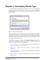
To start performing uncertainty analysis in SNAP, create a new job stream. When
creating the stream, you will be prompted to select a stream type. Select DAKOTA
Uncertainty from this list. This type of stream forms the foundation for uncertainty
analysis in SNAP.
Figure 3.1. Select Stream Type Prompt
After creating the stream, you will need to edit the stream's DAKOTA configuration.
This defines the basic structure of an uncertainty analysis, including how many random
samples must be generated, what figures of merit must be examined, the probability
distributions that define random variates applied to the model, and which random variates
are mapped to which model variables.
The DAKOTA configuration is edited via the Parametric Properties attribute of the
uncertainty stream. Editing this property opens the Edit Uncertainty Configuration
window. The configuration is split across multiple tabs:
•
DAKOTA Properties Tab - the high-level properties for the uncertainty analysis,
such as sample count, figures of merit, and so on.
•
Variables Tab - defines which model variables are mapped to probability
distributions.
•
Probability Distributions Tab - specifies the probability distributions that define the
generated random variates.
•
Report Configuration - configures the OpenDocument Format report generated by
DAKOTA steps.
6
Uncertainty Analysis Plug-ins
Uncertainty Stream Type
The Undo and Redo buttons at the bottom of the editor can be used to revert any changes
made to the configuration since the editor was opened. This history is cleared when the
editor is dismissed.
Press the OK button to accept the changes made to the configuration; if the configuration
is invalid, a prompt will be displayed indicating the error. You can discard changes made
in the editor at any time by either pressing the Cancel button or closing the window.
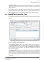
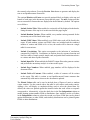
3.1. DAKOTA Properties Tab
The DAKOTA Properties panel implements the high-level properties for the uncertainty
analysis.
Figure 3.2. DAKOTA Basic Configuration
Set the Number of Samples to the number of random samplings applied to the model.
The Calculate Samples button to the right of this field can be used to compute the
required number of tasks for the indicated Order and Probability and Confidence
intervals according to the Wilks method. This calculation is described in more detail in
Wilks Sample Computation.
The Random Seed field can be used to override the seed used to generate pseudo-random
numbers in DAKOTA. Select the check box and enter a value to specify an explicit seed.
When set to a specific value, DAKOTA will generate the same sequence of values every
time the stream is run. If left unset, DAKOTA will generate its own seed based on the
current time.
7
Uncertainty Analysis Plug-ins
Uncertainty Stream Type
Note
Setting the seed will maintain a constant series of variates assuming the rest
of the configuration remains the same. For example, changing the number or
configuration of the probability distributions will change the generated values.
The Sampling Method specifies another constraint on random value generation. With
Monte-Carlo, each random variate is produced from its distribution independent of other
variates; a "good" spread of variates across the distribution is never guaranteed (although
it is likely for a large number of samples). When set to Latin Hypercube, the distribution
is sliced into equally likely bins, and a random value is produced from each bin. The
number of bins is equal to the number of samples needed. By design, the Latin Hypercube
method assures that the distribution will be more easily covered with fewer samples.
Note
Activating the Order value indicates that the order statistic approach is being
used. This disables the sampling method buttons after setting them to MonteCarlo. See Order Statistic Method for more information.
Input Error Handling indicates how the uncertainty stream handles samples that cause
a model to fail its model check. By default, model check errors are ignored and the
sample is used regardless. The stream can also choose to simply filter out any samples
that produce model check errors. The third option uses the Replacement Factor field
to create substitutes for failed samples. When using the replacement strategy for an
uncertainty stream with n samples and a replacement factor of k, the stream will generate
a pool of n+(k*n) inputs. Inputs are taken from this pool, filtering out inputs that fail
model check with errors, until either n samples are selected or the pool is exhausted.
Figures of Merit
A figure-of-merit (FOM) is a single scalar value calculated from the results of a
single analysis code run. The bulk of DAKOTA uncertainty analysis is oriented around
analyzing and correlating FOM values across the parametric tasks (where each task
represent a set of random samples). The Figures of Merit table is used to indicate which
FOMs are expected for uncertainty analysis. The process of extracting the response
values from the data is handled within the stream by the AptPlot Extract Data step (see
AptPlot Data Extraction Step).
Note
"Figure of merit" is approximately synonymous with the term "response
function" found in DAKOTA literature.
Each FOM is defined by an upper and lower limit flag, used to compute the tolerance
interval/limits from the response data. The FOM names and upper/lower limit flags are
edited directly in the table. An uncertainty stream must specify at least one figure of
merit.
Each FOM may also specify a description, which will be carried through to the report
generated by DAKOTA Uncertainty steps (see DAKOTA Uncertainty Step). Editing the
description displays an editing dialog, as shown in Figure 3.3.
8
Uncertainty Analysis Plug-ins
Uncertainty Stream Type
Figure 3.3. Description Dialog
There are two types of description: short and long. The short description is limited to 256
characters and will be shown most places the FOM is referenced, such as above tables
listing the FOM data. Long descriptions may be edited as either an explicit block of text
or as a reference to a model note. The long description is only displayed in the final
section detailing DAKOTA-calculated results for the response, including its cumulative
distribution function, mean, etc.
When Long Description Type is set to Model Note, a set of buttons appear used to edit
the note reference. These buttons are, in order: selecting the note (the selection dialog can
be used to create a new note), edit the referenced note, and create and display a preview
of the note as an OpenDocument Format file. When set to Explicit, a text area appears
in which to enter or edit the long description.
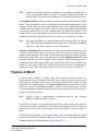
3.2. Variables Tab
Variable definitions control how the input model is varied for each set of random
samples. This tab is composed of a central table, where model variables are mapped to
probability distributions (see Probability Distributions Tab), and table controls used to
add, remove, and reorder rows. The first two columns in the table indicate the name of
the variable and the probability distribution it maps to. The remaining read-only columns
indicate additional values of interest pulled from the referenced variable and probability
distribution.
9
Uncertainty Analysis Plug-ins
Uncertainty Stream Type
Figure 3.4. Model Variables Configuration
Note
The Variable Model column only appears in Engineering Template models.
This column indicates the source model for the indicated variable.
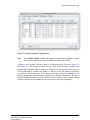
Creating a new variable reference opens a completion dialog, shown in Figure 3.5
and Figure 3.6. This process is broken into two steps. When selecting variables in an
Engineering Template model, a combo box is displayed at the top of the dialog, used to
select which model's variables are displayed. The tree on the left displays a hierarchy
of available variable categories. This category hierarchy is entirely determined by the
plug-in, though most will automatically support user-defined real numerics. The list on
the right displays the model variables for the selected category. Once a model variable
has been selected, the Next button can be used to move on to the second step.
10
Uncertainty Analysis Plug-ins
Uncertainty Stream Type
Figure 3.5. Referencing a model variable: Step 1
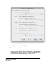
The second step is used to select or create a probability distribution for the reference. You
can select or copy an existing distribution, or create a new distribution with one of the
three variate application rules: Scalar, Additive and Factor. The figure below shows all
available options; model variables may exclude certain application rules, which affects
which choices are actually shown.
11
Uncertainty Analysis Plug-ins
Uncertainty Stream Type
Figure 3.6. Reference a model variable: Step 2
The full list of options are as follows:
•
Select - use a probability distribution that has already been defined. The list of
available distributions will include all factor distributions and any scalar and additive
distributions that have matching units. If the mapped variable does not allow a
certain application rule, distributions of that type will not be listed.
12
Uncertainty Analysis Plug-ins
Uncertainty Stream Type
•
Scalar - create a new scalar distribution, where random variates replace the nominal
value. When this value is selected, the Units drop-down indicates the units that may
be applied to the model variable.
•
Additive - create a new additive distribution, where random variates are added to
the nominal value. Like Scalar, the units for Additive distributions must match the
model variable. See the note below for more information on Additive distribution
units.
•
Factor - create a new factor distribution, where nominal values are multiplied by
randoms variates. Factor distributions do not specify units and can be applied to any
model variable.
•
Copy - copy the selected distribution with a new name. The list of available
distributions follows the same constraints as Select.
The descriptions for the distribution rules illustrate the general case for how random
variates are applied to model variables based on the rule. Individual model variables may
handle them differently, for example setting a mode flag based on the rule while always
replacing the model variable with the variate.
Note
Additive distributions will automatically use "difference" units for units with
offsets in their conversion. For example, a "temperature difference" unit is used
for temperature variables, where 1 degree Kelvin or Celsius is converted to 1.8
degrees Fahrenheit instead of -457.87 and 33.8, respectively. This keeps the
amount added to the nominal value consistent regardless of the unit mode used
in the model. Note that your Additive distribution must still be defined in the
"base" units so that it matches the model variable.
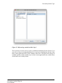
Multiple variables can reference the same probability distribution if necessary. Selecting
cells in the Distribution column displays an editor used to change the reference. Pressing
the editor Select button opens a distribution selection dialog, as shown in Figure 3.7.
13
Uncertainty Analysis Plug-ins
Uncertainty Stream Type
Figure 3.7. Selecting a probability distribution
One random variate is generated per probability distribution definition in each parametric
task, allowing the user the flexibility to consistently apply a single variate across multiple
values.
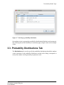
3.3. Probability Distributions Tab
The Distributions tab is used to specify the probability distributions that define random
variate generation. Each probability distribution created in the dialog corresponds to
exactly one random variate generated per parametric task.
14
Uncertainty Analysis Plug-ins
Uncertainty Stream Type
Figure 3.8. Editing the probability distributions
The list on the left shows the distribution. Select an item in the list to display its
properties in the rest of the dialog. The central area is used to modify distribution
properties, including name, type, and type-specific parameters. The uncertainty plug-in
supports the following types of probability distribution: normal (Gaussian), log-normal,
uniform, log-uniform, triangular, exponential, beta, gamma, Gumbel, Frechet, Weibull
and histogram. Type-specific parameters are displayed in the Distribution Parameters
section. Additionally, the right-most section of the tab displays a visualization of the
probability distribution through its density and cumulative distribution functions. The
graphs are updated as the distribution parameters are modified.
Note
The icon next to each distribution is a direct indication of its type. Also, the
model indicator shown in the distribution list only appears in Engineering
Templates.
The normal, log-normal, and triangular distributions allow clipping a probability
distribution via optional Min and Max fields. When the distribution is clipped, the skew
applied to the unbound probability density function is displayed as a blue curve, with the
clipped region shown in gray. The cumulative distribution curve is also adjusted for the
clipped region, as shown in the figure.
New distribution definitions are specified as either a Factor, Additive, or Scalar
distribution, which dictates how a generated random variate is applied to nominal values.
15
Uncertainty Analysis Plug-ins
Uncertainty Stream Type
Figure 3.9. Creating a new probability distribution
The full list of options are as follows:
•
Model - distributions in an Engineering Template model must also specify the model
they apply to. Distributions can only be mapped to variables with matching models.
•
Scalar - create a new scalar distribution, where the random variate replaces the
nominal value. When this value is selected, the Units drop-down is used to select the
units for the new distribution. Distributions may only be matched to model variables
with matching units.
•
Additive - create a new additive distribution, where the random variate is added to
the nominal value. Like Scalar, the units for Additive distributions must be defined.
See the note below for more information on Additive units.
•
Factor - create a new factor distribution, where the random variate is multiplied
against the nomainl value. Factor distributions can be applied to any model variable.
Factor distributions are indicated with a percentage sign (%) next to their name.
•
Copy - copy the selected distribution with a new name.
The descriptions for the distribution rules illustrate the general case for how random
variates are applied to model variables based on the rule. Individual model variables may
16
Uncertainty Analysis Plug-ins
Uncertainty Stream Type
handle them differently, for example setting a mode flag based on the rule while always
replacing the model variable with the variate.
Note
Additive distributions will automatically use "difference" units for units with
offsets in their conversion. For example, a "temperature difference" unit is used
for temperature variables, where 1 degree Kelvin or Celsius is converted to 1.8
degrees Fahrenheit instead of -457.87 and 33.8, respectively. This keeps the
amount added to the nominal value consistent regardless of the unit mode used
in the model. Note that your Additive distribution must still be defined in the
"base" units for those model variables it will map to.
3.4. Report Configuration
The Report tab specifies properties of the report generated by a DAKOTA Uncertainty
step (see DAKOTA Uncertainty Step).
Figure 3.10. Editing the Report Configuration
Title Page allows setting a model note that will be used as the first page shown in the
report. Front Matter is similar: the contents of the selected note will be displayed after
the title page and table of contents. The buttons for both fields have the same functions.
Press the blue Select button to select an existing note. Press the red Edit button to edit
17
Uncertainty Analysis Plug-ins
Uncertainty Stream Type
the currently selected note. Press the Preview Note button to generate and display the
note as an OpenDocument Format file.
The optional Header and Footer text provide optional labels to display at the top and
bottom of each page in the document (except the title page). The misc section provides
access to numerous features that are displayed in the document by default. The options
are as follows:
•
Include Section Titles. When enabled, a section title will be displayed in the header,
listing the name of the top-level section on which the page begins.
•
Include Random Variates. When enabled, every random variate generated for the
uncertainty run will be listed in the report.
•
Include FOM Values. When enabled, every FOM value result will be listed in the
report. If both random variates and FOM values are included and the combined
number of variates and FOMs is five or less, the results will be shown in a single
table for convenience.
•
Include Correlations. This option corresponds to the inclusion of correlations
computed by DAKOTA. Correlations are broken down by response function and
listed as a table of simple, partial, simple rank, and partial rank correlations relative
to variates and other response functions.
•
Include Input File. When enabled, the DAKOTA input file used to generate variates
and perform the uncertainty analysis is written to the report.
•
Include Page Numbers. When enabled, page numbers will be displayed in the
document footer.
•
Include Table of Contents. When enabled, a table of contents will be written
to the report. This table is written as an OpenDocument Format construct that
automatically adds entries whenever the document is updated.
The Plotted Values table can be used to include plots of figures of merit or random
variate samples. Use the controls above the table to add, remove and reorder entries.
Adding a row will display a completion dialog used to select the plotted data. By
default, the values are plotted against the iteration index that each variate or response
corresponds to. Alternatively, select the check-box in the Use Independent column to
enable plotting against another FOM or distribution. Once enabled, use the cell editor
in the Independent column to select the second set of data. FOM data can be plotted
against distributions or other FOMs, and similarly distributions can be plotted against
FOMs or other distributions.
18
Uncertainty Analysis Plug-ins
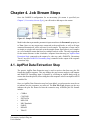
Chapter 4. Job Stream Steps
Once the DAKOTA configuration for an uncertainty job stream is specified (see
Chapter 3, Uncertainty Stream Type), you will need to add steps to the stream.
Figure 4.1. Sample Uncertainty Stream
Model nodes that represent the parametric inputs must have the Parametric property set
to True. Once set, any stream steps connected to the model node, as well as all steps
connected downstream, will be run once for each sample. The sequence of steps can be
as simple as a single code run (such as in the sample stream figure above) or as complex
as a set of multiple restarts that involves multiple analysis codes. The only requirement
for the stream structure is that it includes a response extraction step (see AptPlot Data
Extraction Step) connected to the output of a code step, and a DAKOTA Uncertainty
"fan-in" step (see DAKOTA Uncertainty Step) connected to the output of the response
extractions step.
4.1. AptPlot Data Extraction Step
The generic AptPlot Data Extraction step is used to retrieve data from any plot file
format that AptPlot supports. This step bridges the gap between analysis code outputs
and DAKOTA Uncertainty input. It operates by executing an AptPlot batch script to
extract data from the plot file, then writing the scalar response values in an AptPlot ASCII
variables file.
Once an AptPlot Data Extraction step has been added, several properties must be set
to indicate how the responses are retrieved. The Plot File Type property on the step
indicates the plot file format fed into the extraction step. Available plot file formats
include:
•
•
•
•
•
•
•
•
COBRA
CONTAIN
EXTDATA
MELCOR
NRC Databank
PARCS
RELAP5
TRACE
19
Uncertainty Analysis Plug-ins
Job Stream Steps
Once the file format is specified, the Plot File Data property will need to indicate whether
the plot file has been demultiplexed (a process in which the data is optimized for plotting)
or uses a standard multiplexed plot file. After both of these properties have been set, you
can connect the analysis code step's plot file output to the extract step input.
Note
If you do not see your code listed here, it may use an existing format for its
plot file output, such as EXTDATA. Consult the analysis code user's manual
for more information.
The AptPlot Script property is used to specify the AptPlot batch commands used to
extract response data from the plot file. Editing this property opens a batch command
editor, shown in the figure.
Figure 4.2. Edit Batch Script Dialog
Generated commands bookend the user-specified script; these commands cover opening
the plot file, saving required scalar values (one for each figure of merit requested
by the DAKOTA configuration), and writing the ASCII variable file. The generated
commands cannot be modified. The remainder of the script can be edited to define how
the response data is extracted from the plot file. Consult the AptPlot user's manual for
more information on supported batch script commands.
Note
During stream execution, the ${PlotFile} token is automatically replaced
with the path to the plot file.
Once the script is complete, press the OK button to confirm the changes. You can discard
your modifications at any time by pressing the Cancel button or closing the window.
4.2. DAKOTA Uncertainty Step
The DAKOTA Uncertainty step performs the uncertainty analysis. This is a “fan-in” step:
it takes a file-set produced by a set of parametric steps and runs only once. The DAKOTA
20
Uncertainty Analysis Plug-ins
Job Stream Steps
Uncertainty step, informed by the set of extracted results and a DAKOTA Wrapper XML
file (packaged with the stream by the DAKOTA configuration), aggregates the response
function data into a format understood by DAKOTA, executes DAKOTA in post-run
mode, and organizes the results into the required locations.
The DAKOTA step also creates reports. The uncertainty plug-in generates an
OpenDocument Format (ODF) report detailing the completed uncertainty analysis.
Reports provide a summary of the entire analysis, documenting the configuration input
to DAKOTA, analysis code execution results and the uncertainty and sensitivity results.
ODF has been chosen for its freely available support (ODF can be viewed through the
OpenOffice.org suite, an ODF plug-in for Microsoft Office, etc.).
Generated reports are composed of a formal listing of the DAKOTA configuration
and results, as defined by the DAKOTA configuration (see Report Configuration). The
generation process leverages AptPlot to generate cumulative distribution function plots
of the response for inclusion in the document. Plots of the random variates may also
be included. These extra plots may be defined by either a single variate-generating
probability distribution, which will yield a plot of variates plotted against their iteration
index, or as a pair of distributions, where the variate values for each iteration will form
a complete XY coordinate.
21
Uncertainty Analysis Plug-ins
Appendix A. Wilks Sample
Computation
The Uncertainty Analysis plug-in employs a method for computing sample sizes based
on the Wilks Method, described in the paper Determination of Sample Sizes for Setting
Tolerance Limits by S. S. Wilks. The method is used to determine a number of random
samplings that must be made to assure a certain degree of confidence that a given
probable range of inputs have been covered. The computation has been modified slightly
to account for the order of the order statistic method (see Order Statistic Method).
Given the probability P, confidence C, and number of figures of merit R (aka response
functions), the algorithm for computing the samples is described by the following
pseudo-code:
n = 0
beta = 0
while beta < C
beta = 0
n = n + 1
for j in 0 to n – R
product = innerProduct(...)
beta = beta + product
return n
Where innerProduct(...) is defined as:
When the order of the order statistic (O) is non-zero, and di is the number of bounds on
response function i, the number of response functions (R) is replaced by the following
expression:
22
Uncertainty Analysis Plug-ins
Appendix B. Order Statistic Method
The Order specified in the DAKOTA configuration is used to define a response matrix
created for the DAKOTA Uncertainty report.
The response matrix computation takes several variables as input. It starts out with a
table of response data. Each column in this table represents one figure of merit (FOM),
each row represents a random sampling iteration. From there, the Order value is used to
trim and sort the table based on the upper and lower limit flags for each FOM.
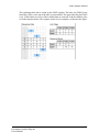
The process for creating the response matrix is best described by example. Consider the
following table data from a hypothetical uncertainty run of twelve samples with three
FOM values per iteration. In this case, we will say that the DAKOTA configuraiton
specifies an order of 2, with upper and lower limit flags (T for true and F for false) as
shown in the figure.
The second figure represents the table after handling FOM1. It starts by sorting table
rows by values in the column for FOM1. Then, since the lower limit flag for FOM1 is
set to true and the order is set to two, the top two rows in the table are removed (these
rows represent the smallest values in FOM1). The number of rows removed at any step
is always equal to the order value. The largest FOM1 value from the clipped rows is set
as the lower value in the response matrix, and the process moves on to FOM2.
23
Uncertainty Analysis Plug-ins
Order Statistic Method
Note
An upper limit value is not defined in the response matrix for FOM1, since the
upper limit flag is set to false.
The third figure represents the table after handling FOM2. Once again, it sorts the
available table rows by values in the column for FOM2 (note that the two rows "removed"
in the previous step did not move and are not considered). As the lower and upper limit
flags for FOM2 are both set to true, two rows are removed from both the top and the
bottom of the remaining data. The lower response value is once again set to the largest
value from the two rows removed at the top, while the upper limit response value is taken
from the smallest value from the two rows removed from at bottom. The response for
FOM2 is now complete, so the process moves on to FOM3.
24
Uncertainty Analysis Plug-ins
Order Statistic Method
The remaining table data is sorted on the FOM3 column. This time, the FOM1 lower
limit flag is false, so the top of the table is not modified. The upper limit flag for FOM3
is set, so the bottom two rows of the available data are removed, with the smallest value
set in the response matrix. The response matrix is now complete, as shown in the figure.
25
Uncertainty Analysis Plug-ins
Index
I
installation, 4
AptPlot, 5
DAKOTA, 4
intro, 1
U
uncertainty analysis, 1
uncertainty steps, 19
AptPlot Data Extract, 19
DAKOTA Uncertainty, 20
uncertainty stream, 6
general, 7
model variables, 9
probability distributions, 14
report configuration, 17
W
Wilks sample computation, 22
26
Uncertainty Analysis Plug-ins