1
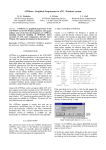
International Conference on Power Systems Transients – IPST 2003 in New Orleans, USA
Implementation of new features in ATPDraw version 3
Hans K. Høidalen1, Bruce A. Mork2, Laszlo Prikler3 , and James L. Hall4
(1) Dept. of Electrical Engineering, the Norwegian University of Science and Technology,
N-7491
Trondheim, Norway (e-mail: [email protected]), (2) Dept. of Electrical Engineering, Michigan
Technological University, Houghton, MI49931-1295, USA, (3) SYSTRAN Engineering Services, Viola u. 7,
H-2013 Pomáz, HUNGARY, (4) Bonneville Power Administration, Portland, OR 97208-3621, USA
II. NEW COMPONENTS
Abstract – The paper addresses the new features in the
ATPDraw program with focus on the technical aspects of
line/cable and transformer modeling. Version 3 of the
program supports directly the supporting routines LINE- and
CABLE CONSTANTS, CABLE PARAMETERS, and
BCTRAN of ATP-EMTP. The paper finally outlines the
advanced, multilevel grouping facility and the new support of
$Parameter and Pocket Calculator.
ATPDraw now directly supports line, cable and
transformer modeling via LINE/CABLE CONSTANTS,
CABLE PARAMETERS and BCTRAN supporting
routines of ATP. The user operates directly with technical
data in the circuit. ATP-EMTP is automatically executed to
produce the electrical models included in the final data
case.
Keywords – Graphical preprocessor, line, cable, and transformer
modeling, CAD, ATP-EMTP
A. Line/cable modeling
To add a line or cable to the circuit, the user first
specifies a 1-9 phase line/cable model. The input dialog
box of this circuit element is shown in fig. 2. In this
dynamic dialog box the user specifies if the component is a
cable (with or without enclosing pipe) or an overhead line.
Then the geometrical and material parameters can be
entered under Data. Under Standard data the ground
resistivity (only homogenous ground supported), the initial
frequency and the line/cable length are specified. Finally
the user selects the suitable electrical model under Model
along with special frequency and fitting data required in
each case. It is straightforward to switch between the
various electrical models (Pi, Bergeron, JMarti, Semlyen,
and Noda) and ATPDraw handles all the formats, apart
from special multiple pi-sections. Only those cases that
really produce an electrical model are supported. Fig. 2
illustrates a JMarti specification of a 750 kV overhead line
given in fig. 3.
In a cable data case the user can easily switch between
CABLE CONSTANTS and CABLE PARAMETERS. The
first supports a flexible grounding scheme and the Semlyen
model, while the second supports additional shunt
capacitance/conductance and the Noda model. For each
cable in the system the user can specify data for the core,
sheath and armor and copy data between cables.
Selecting View will display the cross section. This gives
a quick overview of the system so obvious errors can be
avoided. In the View module zooming is supported as well
as clipboard support of the graphics. This feature is
particularly useful for cable systems as it also shows which
conductor is grounded as illustrated in fig. 4.
I. INTRODUCTION
ATPDraw is a graphical preprocessor to the ATP-EMTP
[1, 2] on the MS Windows platform. In the program the
user can build up an electric circuit, using the mouse, by
selecting predefined components from an extensive palette
[3, 4]. Both single phase and 3-phase components are
supported. ATPDraw generates the ATP file in the proper
format based on "what you see is what you get". ATPDraw
takes care of the node naming process. All kinds of circuit
editing
facilities
(copy/paste,
grouping,
rotate,
export/import, undo/redo) are available. Most of ATP’s
standard components as well as TACS are supported, and
in addition the user can create new objects based on
MODELS [5] or Data Base Modularization [1]. ATPDraw
has a standard Windows layout, supports multiple
documents and offers a large Windows help file system.
Fig. 1. Layout of ATPDraw's main screen, including the
component selection menu
1
International Conference on Power Systems Transients – IPST 2003 in New Orleans, USA
corrections could be to change the frequency for which the
transformation matrix is calculated at.
Fig. 4. Specification of Cable data under Cable Parameters
(grounding is fixed) and View of the cross section. Grounded
conductors appear in the background color.
Fig. 2. Line/Cable dialog box. Upper: Selection of system type
(line or cable), standard data (grounding and frequency) and
Model data (type of model and frequency). Lower: Specification
of conductor data.
13.2 m
At tower
= 41.05 m
Midspan
= 26.15 m
Fig. 5. Verification of the JMarti line in fig. 2, positive sequence.
The accuracy is highest around the transformation matrix
frequency (Freq. matrix ) 1000 Hz.
At tower
= 27.9 m
Midspan
= 13.0 m
17.5 m
Separ=60 cm
Alpha=45 °
NB=4
Fig. 3. Cross section of 750 kV overhead line.
An important part is the Verify module that supports two
method of model verification. The first one is called LINE
MODEL FREQUENCY SCAN [1]. This method compares
the model with the exact PI-equivalent in the frequency
domain. Calculation of impedances in the zero and positive
sequence and the mutual sequence impedance between two
circuits of 6-phase systems is supported. The user can
specify which circuit the conductors belong to and
optionally ground conductors. Fig. 5 shows the verification
of the model in fig. 2-3. The method can be used to verify
if the model is suitable for the typical transients occurring
in the study. For the JMarti line verified in fig. 5
Fig. 6. Verification of the 750 kV power line in fig. 2-3.
The second method is called POWER FREQUENCY
CALCULATION. This method calculates the short circuit
impedances and the open circuit reactive power charging
in the zero and positive sequence as well as mutual transfer
impedance for multi-circuit systems at power frequency.
Such values are typically available benchmark data for
systems in operation. Fig. 6 shows the verification of the
model in fig. 2-3. The method can be used to verify if the
2
International Conference on Power Systems Transients – IPST 2003 in New Orleans, USA
parameters used for the system is correct. Typical
problems could be overhead line heights and ground
resistivity etc.
When the user clicks on the Run ATP or the OK button
of the Line/Cable dialog box (fig. 2) ATPDraw executes
ATP and automatically transforms the punched file into a
library file on data base module format ready to be used in
the electrical circuit.
2
æ VH ö
÷÷
Z *H - L = Z L - H × çç
è VH - VL ø
(1)
Z *L -T = Z L -T
×
×
Z
V
V
Z
×
V
Z
×
V
Z *H -T = H - L H 2 L + H -T H + L -T L
VH - VL
VH - VL
(V H - V L )
where ZL-H, ZL-T, and ZH-T are the Imp. [%] values from
*
*
fig. 7 (lower) and Z H - L , Z L -T , and
written to the BCTRAN file.
B. Transformer modeling
Z H* -T are the values
In version 3.5 of ATPDraw, BCTRAN is supported
directly in the same way as lines/cables. ATPDraw
supports single and 3-phase transformers with up to 3
windings. All types of phase shifts for D- and Y-connected
windings are supported, and a special handling of autotransformers is included. Handling of the nonlinear
magnetization branch is also incorporated both manually
and automatic. In a new View module the user can get a
picture of the nonlinear characteristic and easily transforms
the voltage/current rms-value characteristic into a
fluxlinked/peak-current characteristic.
Fig. 7 shows the BCTRAN dialog box with data based
on the test report of a 290 MVA transformer shown in
table I.
Table I Transformer test report, 290 MVA 50 Hz.
Main
data
[kV]
HS
LS
Open
circuit test
LS
432
16
[A]
Coupling
290
290
E0 [kV] (%) [MVA]
388
10465
I0 [%]
YNj
d5
P0 [kW]
12 (75)
14 (87.5)
15 (93.75)
16 (100)
17 (106.25)
[kV]
290
290
290
290
290
[MVA]
0.05
0.11
0.17
0.31
0.67
ek, er [%]
83.1
118.8
143.6
178.6
226.5
Pk [kW]
290
14.6, 0.24
704.4
Short
circuit test
HS/LS
432/16
[MVA]
Fig. 7. BCTRAN dialog box. Specification of data according to
tab. I. Upper: Open circuit data. Lower: Short circuit data
Under Factory test the user can choose either the open
circuit test or the short circuit test as shown in fig. 7. Under
the open circuit test the user can specify where the test was
performed and where to connect the excitation branch.
Normally the lowest voltage is preferred, but stability
problems for delta-connected nonlinear inductances could
require the lowest Y-connected winding to be used. The
user can choose between the HV and LV, and TV winding
for a three-winding transformer. The excitation voltage and
current is specified in % and the losses in kW. With
reference to the ATP RuleBook [1], the values at 100 %
voltage is used directly as IEXPOS=Curr [%] and
LEXPOS=Loss [kW]. The user can specify up to 6 point
on the magnetizing curve.
The reference current in the open circuit case is
I ref = 290 MVA/( 3 × 16 kV) = 10.5 kA
Under Structure in fig. 7, the user specifies the number
of phases, the number of windings, the type of core (not
supported yet, except for single-phase cores, triplex), and
the test frequency. The dialog box format adapts the
number of windings and phases. The user can also request
the inverse L matrix as output by checking AR Output. An
Auto-add nonlinearities button appears when an external
magnetizing branch is requested as explained below.
Under Ratings the nominal line-voltage, rated power,
and type of coupling is specified. Connections A (autotransformer), Y and D are available and all possible phase
shifts are supported. The specified line voltage is
automatically scaled to get the winding voltage VRAT. If
an Auto-transformer is selected for the primary and
secondary winding (HV-LV) the impedances are
recalculated as shown in section 6.7 in [2]:
C. Nonlinearities
How to handle the nonlinear open circuit characteristic
is specified under the Positive core magnetization group in
fig. 7. Specifying Linear internal will result in a linear core
representation based on the 100 % voltage values. It is also
3
International Conference on Power Systems Transients – IPST 2003 in New Orleans, USA
The calculated Irms-Urms characteristic can be
automatically transformed to an i-l (current-fluxlinked)
characteristic (by an internal SATURA-like routine [1, 2]).
Selecting the Lm-flux will allow to display the i-l
characteristic similar to fig. 9, and to copy it directly to
nonlinear inductances of type 93 and 98.
The user can choose to Auto-add nonlinearities under
Structure and in this case the magnetizing inductance is
automatically added to the final ATP-file as a type 98
inductance. ATPDraw connects the inductances in Y or D
dependent on the selected connection for actual winding
for a 3-phase transformer. In this case the user has no
control of the initial state of the inductor(s). If more control
is needed Auto-add nonlinearities should not be checked.
The user must then create separate nonlinear inductances
and copy the i-l characteristic.
possible to handle the saturation. Typically the
magnetization inductance can be added externally. To
accomplish this the user has to select External Lm. The
inductive part of the magnetization current at 100 %
voltage is then subtracted and the remaining open circuit
current becomes equal to the resistive part:
IEXPOS[%] = 100 × ( P × 10 -3 [ MVA] /( SPOS[ MVA]) (2)
= 178.6 /(10 × 290) = 0.0616%
where SPOS is equal to the Power [MVA] specified
under Ratings for the winding where the test is performed,
and P is equal to the open circuit Loss [kW] at 100 %
voltage. The current in the magnetizing inductance, ref.
fig. 8 is then calculated as
I rms [ A] =
10 × SPOS [ MVA]
3 × Vref [kV ]
(Curr[%])2 - æçç
Loss[kW ] ö
÷÷
è 10 × SPOS [ MVA] ø
2
(3)
Fig. 10 shows a simulation of the open circuit excitation
current into the low voltage side, applying 16 kV line
voltage.
where Vref is actual rated voltage specified under
Ratings, divided by
3 for 3-phase Y- and Autoconnected transformers. Curr, Loss, and Volt are taken
directly from the open circuit data. The factor 3 in (3) is
used only for the 3-phase case. The Urms values are then
Volt [%]
× Vref [kV ]
(4)
calculated as U rms =
100
50.0
[A]
37.5
ITA
ILA
IBCT
ILA-C
25.0
12.5
Irms
0.0
Urms
IBCT ITA
-12.5
BCT
-25.0
Fig. 8. Definition of the Irms-Urms quantities.
ILA
-37.5
Selecting Lm-rms under the View/Copy group and then
the button View+ will display the nonlinear characteristic
for the positive sequence system as shown in fig. 9.
-50.0
0
5
10
15
[ms]
20
Fig. 10. Open circuit currents at nominal voltage.
Fig. 11 shows the measured no-load current of the at the
same transformer. The line-current in phase A is shown
together with the phase current A to C. This figure fits
qualitively well with fig. 10. The peaks of the line-current
are a bit higher, particularly the second peak on the
positive part that is produced by the phase current ILA-C.
The current in phase A into the D-coupled inductors, ILA
shown in fig. 10 consists of two peaks each half period.
The first one comes from the current in the inductance in
branch A-B (ILA-B) and the second one comes from branch
A-C. In (3) it is assumed that the current in each saturation
inductor for a D-connected winding is equal to the phase
current divided by 3 . This is a doubtful assumption
however, since the three involved inductances will go into
saturation at different times.
Nonlinear inductances with initial fluxlinked condition
are added to ATPDraw. This is straightforward for type 93
inductances while type 96 and 98 require special treatment.
A hidden DC voltage source is connected in series with the
inductor lasting for one time step and with amplitude of
l(0)/dt where l(0) is the user specified initial fluxlinked
Fig. 9. Viewing the magnetization characteristic.
A similar characteristic can also be calculated for the
resistive part. If zero sequence data are available they can
be specified in fig. 7 as well.
4
International Conference on Power Systems Transients – IPST 2003 in New Orleans, USA
condition. The voltage source (and the required ideal
transformer for non-grounded inductances) is hidden in the
graphical drawing.
in
out
60
ITA
ILA-C
[A]
40
Fig. 12 Compressing a 3-phase rms-meter in TACS.
20
Fig. 13 shows a more advanced case where a 6-pulse
thyristor bridge with TACS control [6] is grouped into a
single object with the AC-frequency, the firing delay angle
and the RC values of the snubber-circuits as data
parameters. This is equal to example Exe_6g.adp in the
ATPDraw distribution.
0
-20
-40
POS
-60
0
5
10
15
1
3
5
4
6
2
Freq
Freq
20
[ms]
Fig. 11. Measurement of excitation currents at nominal voltage.
Angle
NEG
180
In addition these components offer the user to select
the fluxlinked output just like any other branch output. To
support this ATPDraw adds a TACS branch voltage
integrator automatically. Also an extra node will appear
where the user can specify the fluxlinked name.
III. NEW EDIT OPTIONS
Fig. 13. 6-pulse Thyristor Bridge grouped into a single object.
Two new mayor edit options were added to ATPDraw
version 3. These are multilevel grouping and support of
text string parameters.
B. Parameters
ATPDraw version 3 supports ATP's $Parameters and
Pocket Calculator. This implies that the user can specify a
6-character text string for most data parameters and later
assign a value to this variable globally. This is particularly
useful when a data value is used several times in a circuit.
In such a case all equal data parameters could be given the
same text string name. The time consuming and risky
procedure of clicking up a lot of windows to change the
common value can thus be avoided. ATPDraw takes care
optimal resolution by adding '_' characters to the text
string.
The Pocket Calculator feature allows a data value to be a
function of the simulation number in a multiple run. Fig.
14 shows an example where the rms value of the open
circuit current for the transformer model in fig. 7 is
calculated as a function of the excitation voltage from 1217 kV. The External Lm and the Auto-add nonlinearities
options are selected.
The amplitude of the voltage source is given the text
string variable 'AMP'. This variable is then later assign a
value under ATP|Settings as shown in fig. 15. The Number
of simulations is set to 6 and this will enable the Pocket
Calculator feature. The amplitude is defined as a function
of the simulation number KNT. The constant value 816.5
is equal to 1000 × 2 / 3 .
A. Grouping
This option is a powerful tool to increase the readability
of the circuit drawings and for reuse of frequent subcircuits. Typical examples are grouping of TACS blocks
into control system units and creation of 3-phase
components. A group can be exported and imported
making it possible to build up a library of frequent used
sub-circuits. ATPDraw supports multilevel grouping.
The grouping process is called Compress and the user is
free to select which of the data and nodes to be external
and accessible from the outside. If two data parameters are
given the same name they seen as one from the outside. It
is also possible to let a nonlinear characteristic become
external.
A simple example is shown in fig. 12 where a 3-phase
rms-meter is constructed. The user first selects a group,
then Edit|Compress. In this dialog box the external
data/nodes are specified. Finally, a single default icon (that
can be modified) replaces the sub-circuit. The data
parameters are the frequency used in the TACS device 66
and the type of input (voltage=90, current=91) to TACS
for the three phases. These show up as only two parameters
in the final rms-meter object.
5
International Conference on Power Systems Transients – IPST 2003 in New Orleans, USA
special/miscellaneous ATP options like ABSOLUTE
U.M. DIMENSIONS etc.
· The file system is substantially changed. The ATPDraw
distribution consists of 4 files (along with the examples);
The executable program, two help files and the standard
component library (ATPDraw.scl) which contains the
format of about 200 standard components. The user save
his work in a project file, which contains all the files
required to edit, run, and distribute the data case.
· A User’s Manual [3] that documents ATPDraw version
is divided in six parts. Parts 1-3 introduce ATPDraw and
explain how to get started with the program. Part 4 is a
Reference manual for all menus and components. Part 5
is the Advanced manual that covers the new features
presented in this paper, along with how to create new
components (Modules or MODELS). Part 6 is an
Application manual with several practical examples.
U
Fig. 14. ATPDraw-circuit for calculation of rms-values.
IV. DISCUSSION/CONCLUSION
ATPDraw version 3 covers line, cable, and transformer
modeling. The Verify part of overhead lines functions well,
while problems still exist for cable systems. Verification of
Noda models is not supported. The support of BCTRAN
still needs improvements and increased knowledge about
how to handle 3-legged cores and D-connected
magnetizing branches, including the nonlinearity in the
magnetization losses. Saturation can be automatically
added externally to the BCTRAN linear matrix model
connected and in D- or Y-couplings. D-coupled nonlinear
inductances can some times cause numerical problems so
connecting the magnetization branch at the Y-coupled
winding closest to the core is recommended.
The new edit features Grouping and Parameters simplify
and open up new possibilities in modular circuit
construction.
Fig. 15. Assigning a value to the text string 'AMP'.
Fig. 16 compares the measured rms-values of the open
circuit currents (from tab. I) with the calculated (from fig.
14). The resistive part of the magnetizing branch is fixed at
the 100 % voltage value.
80
Meas Calc
I0 [Arms]
60
40
ACKNOWLEDGEMENT
20
The work on ATPDraw is possible due to financing
from U.S. Dept. of Energy, Bonneville Power
Administration and Pacific Engineering Corporation.
Francisco Gonzalez Molina and Sung Don Cho advised the
development of the BCTRAN support.
U0 [kV]
0
12
13
14
15
16
17
Fig. 16. Comparison of measured and calculated rms-values of
open circuit currents.
REFERENCES
C. Other options
ATPDraw version 3 also supports some other new
features. Among these are
· Rubber-band connections. When this option is selected,
connections behave like rubber-bands and follows a
moving component/group. This is useful when larger
parts of a circuit are moved.
· Automatic lis-file error detection. After the ATP
execution the lis-file can be automatically examined for
error/warning messages. The user can select 5 different
and typical flags.
· Free format ATP-file input. The user now has the option
to insert text strings directly into the ATP-file at
predefined positions. These text-strings follow the
project file. This will enable an indirect support of
[1] Alternative Transients Program (ATP) - Rule Book,
Canadian/American EMTP User Group, 1987-1998.
[2] H. W. Dommel et.al., Electromagnetic Transients Program
Reference Manual (EMTP Theory Book, Prepared for BPA,
Aug. 1986.
[3] L. Prikler, H.K. Høidalen, ATPDraw version 3.5 for Windows
9x/NT/2000/XP User’s Manual, SEfAS TR F5680, ISBN 82594-2344-8, Aug. 2002.
[4] H. K. Høidalen, L. Prikler, J.Hall, "ATPDraw- Graphical
Preprocessor to ATP. Windows version", Proc. IPST,
pp. 7-12, June 20-24, 1999, Budapest-Hungary.
[5] L. Dubé, Models in ATP, Language manual, Feb. 1996.
[6] N. Mohan, Computer Exercises for Power Electronics
Education, Dept. Electrical Engineering, University of
Minnesota, 1990.
6