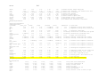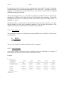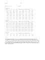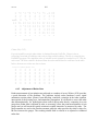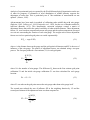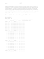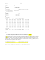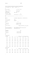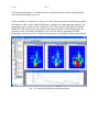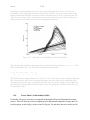
1
WATFLOOD / WATROUTE Hydrological Model Routing & Flow Forecasting System SINCE 1972 Developed for Surveys and Information Branch Ecosystem Science and Evaluation Directorate ENVIRONMENT CANADA by Nicholas Kouwen, Ph.D., P.Eng., F.ASCE Distinguished Professor Emeritous Department of Civil Engineering University of Waterloo Waterloo, Ontario, Canada N2L 3G1 519-922-2602 E-mail: kouwen@ uwaterloo.ca http://www.watflood.ca First Edition: March 1986 Last Revision: Sep., 2014 Copyright (C) by N. Kouwen, 1986 - 2014 (This manual may be reproduced whole or in part providing acknowledgements are given.) Jan. 2014 ii IMPORTANT NOTE: WATFLOOD programs now read onlyGreenKenue format files. Old file formats are no longer supported. A program called trns.exe can convert old formats to theGreenKenue formats. See Chapter 14 DISCLAIMER The WATFLOOD software is furnished by N. Kouwen and the University of Waterloo and is accepted and used by the recipient upon the express understanding that N. Kouwen and the University of Waterloo make no warranties, either express or implied, concerning the accuracy, completeness, reliability, usability, performance, or fitness for any particular purpose or the information contained in this manual, to the software described in this manual, and to other material supplied in connection therewith. The material is provided "as is". The entire risk as to its quality and performance is with the user. The forecasts produced by the WATFLOOD software are for information and discussion purposes only and are not to be relied upon in any particular situation without the express written consent of N. Kouwen or the University of Waterloo. Jan. 2014 iii WATFLOOD - with Grouped Response Units WATFLOOD is an integrated set of computer programs to forecast flood flows or do simulations for watersheds having response times ranging from one hour to several weeks. Continuous long term simulation can be carried out by chaining events. The emphasis of the WATFLOOD system is on making optimal use of remotely sensed data, radar-rainfall data, LANDSAT or SPOT land use and/or land cover data can thus be directly incorporated in the hydrologic modeling. WATFLOOD is the first hydrological model to preserve the distributed nature of a watershed's hydrologic and meteorological variability without sacrificing computational efficiency. This has been accomplished through the use of Grouped Response Units, in which process parameters are tied to land cover and land cover mixes can vary from basin element to basin element. This approach is becoming more popular each year. The basic premise of the GRU method is that vegetation and/or land use is the predominant hydrological indicator of hydrological response. The system is completely modular but has a consistent data structure throughout. It has been under continuous development since 1972. Several Master and Ph.D. research programs have provided the rationale incorporated in the software but programs have all been written or adapted by the author. Jan. 2014 iv TABLE OF CONTENTS 1. WATFLOOD USER’S MANUAL ........................................................................ 1-1 1.1. Introduction ................................................................................................................................................ 1-1 1.2. Approach ..................................................................................................................................................... 1-1 1.3. Getting Started ........................................................................................................................................... 1-4 1.3.1 Overview ............................................................................................................................................. 1-4 1.3.2 Installation - WINDOWS .................................................................................................................... 1-5 1.3.3 Installation DOS: ................................................................................................................................. 1-5 1.3.4 File Structure in WATFLOOD ............................................................................................................ 1-6 1.3.5 Minimum File Requirements ............................................................................................................... 1-7 1.3.6 File Naming Convention ...................................................................................................................... 1-8 1.3.7 GREENKENUE compatibility ............................................................................................................ 1-8 1.3.8 Event Configuration File (event\yyyymmdd.evt) ................................................................................ 1-9 1.3.9 Meaning of the flags in the event file ................................................................................................ 1-13 1.3.10 Multiple Events for Continuous Modelling (Chaining) ..................................................................... 1-15 1.3.11 Creating event files ............................................................................................................................ 1-15 1.4. WATFLOOD TUTORIAL ...................................................................................................................... 1-19 1.4.1 WATFLOOD for WINDOWS - SADLY, IT’s GONE ................................................................... 1-19 1.4.2 DOS (Disk Operating System)........................................................................................................... 1-19 1.4.3 Use Existing Event (e.g., Demonstration Program) ........................................................................... 1-20 1.4.4 Create New Event (inactive) ............................................................................................................. 1-20 1.4.5 Demonstration.................................................................................................................................... 1-20 1.4.6 Editing Files ....................................................................................................................................... 1-21 1.4.7 Initiating Snow Accounting ............................................................................................................... 1-21 1.4.8 Scale Factors ...................................................................................................................................... 1-23 1.5. WATFLOOD Programs - file requirements .......................................................................................... 1-24 1.5.1 Read CAPPI (RADMET) ................................................................................................................. 1-25 1.5.2 Adjust (or Calibrate) Radar Data (CALMET) ................................................................................... 1-25 1.5.3 Distribute Rainfall Data (RAGMET)................................................................................................. 1-25 1.5.4 Distribute Snow Course Data (SNW) ................................................................................................ 1-27 1.5.5 Distribute Soil Moisture Data (MOIST) ............................................................................................ 1-27 1.5.6 Distribute Temperature Data (TMP) .................................................................................................. 1-27 1.5.7 Run SPL9 (SPL) ................................................................................................................................ 1-27 1.5.8 Single Event Mode ............................................................................................................................ 1-28 1.5.9 Forecast Without Optimization Mode ............................................................................................... 1-28 1.5.10 Forecast With Optimization Mode..................................................................................................... 1-28 1.5.11 Model Calibration Mode.................................................................................................................... 1-28 1.5.12 Debug Mode ...................................................................................................................................... 1-29 1.5.13 Forecast Mode Without RADAR Image Scaling ............................................................................... 1-29 1.5.14 Forecast Mode With RADAR Image Scaling .................................................................................... 1-29 1.5.15 Stage Hydrographs (STGPLT) (Provisional) ..................................................................................... 1-30 1.5.16 Flow Animation in GreenKenue ........................................................................................................ 1-31 1.6. Setting Up a New Event (Out of order) .................................................................................................. 1-32 1.7. Debugging SPL ......................................................................................................................................... 1-34 1.7.1 Common Problems ............................................................................................................................ 1-34 Jan. 2014 v 1.8. Output Files............................................................................................................................................... 1-36 1.9.1 Do’s ................................................................................................................................................... 1-39 1.9.2 Don’t’s ............................................................................................................................................... 1-40 1.9. Known problems ....................................................................................................................................... 1-40 1.10. Help (free for students – others: not so much) ...................................................................................... 1-40 2. HYDROLOGICAL MODEL ................................................................................ 2-1 2.1. Introduction ................................................................................................................................................ 2-1 2.2. Modeling Aspects ........................................................................................................................................ 2-1 2.2.1 Surface Storage .................................................................................................................................... 2-2 2.2.2 Infiltration ............................................................................................................................................ 2-3 2.2.3 Initial Soil Moisture ............................................................................................................................. 2-5 2.3. Potential Evapotranspiration .................................................................................................................... 2-5 2.3.1 Priestley - Taylor Equation .................................................................................................................. 2-6 2.3.2 Hargreaves Equation ............................................................................................................................ 2-7 2.4. Actual Evapotranspiration (by T. Neff.)................................................................................................. 2-9 2.4.1 Soil Moisture Coefficient..................................................................................................................... 2-9 2.4.2 Soil Temperature Coefficient............................................................................................................. 2-10 2.4.3 Forest Vegetation CoefficientFTALL................................................................................................ 2-10 2.4.4 Calculating AET from PET – land classes......................................................................................... 2-11 2.4.5 Calculating AET – water class (lakes) ............................................................................................... 2-11 2.5. Interception (by T. Neff.) ....................................................................................................................... 2-11 2.6. Interflow .................................................................................................................................................... 2-13 2.7. UZ to LZ Drainage (or Ground Water Recharge) ................................................................................ 2-14 2.8. Overland flow ........................................................................................................................................... 2-14 2.9. Base Flow................................................................................................................................................... 2-15 2.10. Total Runoff .............................................................................................................................................. 2-16 2.11. Routing Model .......................................................................................................................................... 2-16 2.11.1 Main channel flow: ............................................................................................................................ 2-17 2.11.2 Channel flow & overbank flow: ........................................................................................................ 2-18 2.11.3 Lake effect on routing <<new ......................................................................................................... 2-18 2.11.4 Bankfull – Drainage area relationship ............................................................................................... 2-18 2.12. Wetland Routing (Bank Storage Model) ................................................................................................ 2-19 2.12.1 Wetlands - Fens and Bogs ................................................................................................................. 2-21 2.13. Lake Routing............................................................................................................................................. 2-21 2.13.1 Reservoirs and Large Lakes ............................................................................................................... 2-21 2.13.2 Instream Lakes (numerous) ............................................................................................................... 2-22 2.14. Lake Evaporation ..................................................................................................................................... 2-22 Jan. 2014 vi 2.15. Snowmelt Model ....................................................................................................................................... 2-23 2.15.1 Temperature Index Model ................................................................................................................. 2-23 2.15.2 Radiation-Temperature Index Algorithm........................................................................................... 2-25 3. WATERSHED DATA REQUIREMENTS............................................................ 3-1 3.1. Georeference Requirements ...................................................................................................................... 3-1 3.2. Setting Up a New Watershed ..................................................................................................................... 3-1 3.2.1 Mandatory Files (Summary) ................................................................................................................ 3-2 3.2.2 Steps to Set Up a New Watershed ....................................................................................................... 3-3 3.2.3 Watershed Data .................................................................................................................................... 3-4 3.3. Basin File ..................................................................................................................................................... 3-5 3.3.1 Entering Watershed Coordinates ......................................................................................................... 3-5 3.3.2 Data Separators (Headings) ................................................................................................................. 3-8 3.3.3 River Invert Elevation (ELV) .............................................................................................................. 3-8 3.3.4 Grid Drainage Area (FRAC).............................................................................................................. 3-10 3.3.5 Drainage Directions (S) ..................................................................................................................... 3-10 3.3.6 River Classification (IBN) ................................................................................................................. 3-11 3.3.7 Contour Density (IROUGH) .............................................................................................................. 3-11 3.3.8 Channel Density (ICHNL) ................................................................................................................. 3-12 3.3.9 Routing Reach Number (IREACH) ................................................................................................... 3-13 3.3.10 Fetch (8 directions) <<new !! ........................................................................................................... 3-13 3.3.11 Land Cover Classes (IAK) ................................................................................................................. 3-15 3.3.12 Class Numbering - order of entering land cover classes .................................................................... 3-17 3.3.13 Wetlands – Splitting Bogs and Fens .................................................................................................. 3-17 3.3.14 Combining and Reordering Classes ................................................................................................... 3-18 3.3.15 Non-Contributing Areas .................................................................................................................... 3-20 3.3.16 Basin File (bsnm_SHD.r2c) for UTM Coordinates ......................................................................... 3-23 3.3.17 Basin File (.SHD) for UTM Coordinates ......................................................................................... 3-30 3.3.18 Basin File for Geographical Coordinates (LATLONG) .................................................................... 3-34 3.4. Setting up Sub-watersheds << new!! ...................................................................................................... 3-34 3.4.1 Creating a sub-watershed subbsnm_shd.r2c file << new!! .............................................................. 3-34 3.4.2 Creating reduced met & tmp files << new!! .................................................................................... 3-35 3.5. Additional Required Files ........................................................................................................................ 3-36 3.5.1 BSNM.PDL File for UTM Coordinates............................................................................................. 3-36 3.6. Additional Optional Files (New 2012) ..................................................................................................... 3-38 3.6.1 Optional Storage-Discharge curves for lakes & reservoirs ................................................................ 3-38 3.6.2 BSNM.PAR File ................................................................................................................................ 3-39 3.6.3 CALMET.PAR File ........................................................................................................................... 3-39 3.7. Mean and Max grid elevations for lapse rate applications - New ........................................................ 3-39 3.8. Watershed data summary ........................................................................................................................ 3-40 4. MODEL PARAMETERS AND OPTIMIZATION ................................................. 4-1 4.1. Parameter File ............................................................................................................................................ 4-1 4.2. General Parameters in the .par File .......................................................................................................... 4-9 vii Jan. 2014 4.2.1 4.2.2 4.2.3 4.2.4 4.2.5 4.2.6 Example of Global Parameters .......................................................................................................... 4-11 River and Basin parameters ............................................................................................................... 4-12 Hydrological (Surface) Parameters .................................................................................................... 4-12 Snowmelt Parameters ........................................................................................................................ 4-14 Monthly ET data ................................................................................................................................ 4-14 Interception Parameters ..................................................................................................................... 4-15 4.3. Monthly_climate_normals (replaced by daily temperature differences Jan. 2014)............................ 4-15 4.4. Snow Cover Depletion Curve (SDC) ....................................................................................................... 4-15 4.5. Optimization (Updated April 10, 2010) .................................................................................................. 4-17 4.5.1 Hints for Successful Optimization ..................................................................................................... 4-17 4.5.2 Pattern Search .................................................................................................................................... 4-18 4.5.3 Optimization – Dynamically Dimensioned Search DDS ................................................................... 4-21 4.5.4 Optimization Hints............................................................................................................................. 4-30 4.5.5 Pattern Search (Currently not operational) ........................................................................................ 4-31 4.5.6 Dynamically Dimensioned Search DDS ............................................................................................ 4-36 4.6. Trouble shooting ....................................................................................................................................... 4-36 4.7. Parameter Sensitivity Analysis (beta version)........................................................................................ 4-39 5. MODEL INITIALIZATION................................................................................... 5-1 5.1. Initial Snow Cover ...................................................................................................................................... 5-1 5.1.1 Sample Initial Point Snow Water Equivalent File ( yyyynndd_crs.pt2): ............................................. 5-1 5.1.2 Sample of Gridded Snow Water Equivalent Map ................................................................................ 5-2 5.2. Initial Soil Moisture.................................................................................................................................... 5-4 5.3. Sample Point Initial Soil Moisture File (_PSM.r2c) (Soild moisture Data):.......................................... 5-4 5.4. Sample of Gridded Initial Soil Moisture Map (_gsm.r2c)....................................................................... 5-5 5.5. Initial Channel Storage .............................................................................................................................. 5-6 5.6. Initial Lower Zone Storage ........................................................................................................................ 5-6 6. RAINFALL DATA PROCESSING ...................................................................... 6-1 6.1. Introduction ................................................................................................................................................ 6-1 6.1.1 Rain Gauge Data File (_RAG.tb0)....................................................................................................... 6-2 6.1.2 Distribution of Gauge Precipitation ..................................................................................................... 6-3 6.1.3 Modified Distribution of Precipitation................................................................................................. 6-4 6.1.4 Precipitation lapse rate (rlapse)............................................................................................................ 6-5 6.2. Disaggregation of rainfall (smrflg=y)........................................................................................................ 6-5 6.3. Precipitation Data (yyyymmdd_met.r2c) - Input to SPL ....................................................................... 6-6 6.4. Radar Precipitation Data ........................................................................................................................... 6-8 6.4.1 Unadjusted Radar File (.RAD) ............................................................................................................ 6-8 6.4.2 Adjustment of Radar Data ................................................................................................................... 6-9 viii Jan. 2014 6.4.3 6.4.4 7. CALMET.PAR File ........................................................................................................................... 6-11 Calibrated Radar File (_MET.r2c) ..................................................................................................... 6-11 FLOW DATA ...................................................................................................... 7-1 7.1. Streamflow Files ......................................................................................................................................... 7-1 7.1.1 Example streamflow file ...................................................................................................................... 7-1 7.1.2 Water Survey Card format ................................................................................................................... 7-3 7.1.3 Observed Stage Input – Under construction ........................................................................................ 7-4 7.1.4 Flow Station Area Check ..................................................................................................................... 7-4 7.2. Reservoir Release File ................................................................................................................................ 7-5 7.2.1 Natural lake and uncontrolled reservoirs ............................................................................................. 7-7 7.2.2 Initial reservoir levels .......................................................................................................................... 7-8 7.2.3 Natural flows ....................................................................................................................................... 7-9 7.3. Reservoir Inflow Files ................................................................................................................................ 7-9 7.4. Diversions (BETA Jan/09) ....................................................................................................................... 7-10 8. TEMPERATURE DATA ..................................................................................... 8-1 8.1. Example of Point Temperature File: ........................................................................................................ 8-1 8.2. Modified Distribution of temperature ...................................................................................................... 8-2 8.3. Temperature lapse rate (tlapse) ................................................................................................................ 8-3 8.4. Example of a Gridded Temperature File tempr\yyyymmdd_tem.r2c ................................................. 8-3 8.5. Daily Temperature Differences (for ET calculations) << new!! ............................................................ 8-4 9. RADIATION DATA............................................................................................. 9-1 10. OUTPUT FILES ............................................................................................... 10-1 10.1. Plotting hydrographs (observed vs. computed) ..................................................................................... 10-3 10.2. Spl.txt File – IOPT=1 ............................................................................................................................... 10-4 10.2.1 File Names from the Event File ......................................................................................................... 10-4 10.2.2 Land cover by Sub-basin .................................................................................................................. 10-5 10.2.3 Information on Flags.......................................................................................................................... 10-5 10.2.4 Reservoir Locations and Operating Rules ......................................................................................... 10-5 10.2.5 Information for Each Grid ................................................................................................................. 10-5 10.2.6 Summary for Grids ............................................................................................................................ 10-6 10.2.7 Cummilative Statistics for Each Event .............................................................................................. 10-7 10.2.8 Repeated for Each Event.................................................................................................................... 10-7 10.2.9 Gridded channel flows Spl_flow.r2c ................................................................................................. 10-8 10.2.10 Supplementary files ........................................................................................................................... 10-8 10.3. Rff.txt File ................................................................................................................................................. 10-8 Jan. 2014 ix 10.4. Outfiles.txt File ....................................................................................................................................... 10-10 11. WATROUTE..................................................................................................... 11-1 11.1. How to use WATROUTE......................................................................................................................... 11-5 11.2. RUNOFF (_rff) RECHARGE (_rch) and and LEAKAGE (_lkg) file creation with WATFLOOD . 11-6 11.3. Recharge files for MODFLOW ............................................................................................................. 11-11 11.4. WATROUTE output >>NEW<< ........................................................................................................... 11-12 11.5. Combining WATFLOOD runoff and MODFLOW leakage .............................................................. 11-12 12. INTERFACING WITH GREENKENUE........................................................... 12-13 12.1. How to debug with GreenKenue: .......................................................................................................... 12-15 13. WATFLOOD OPTIONS.................................................................................... 13-1 13.1. Precipitation Adjustment File (PAF) ...................................................................................................... 13-1 13.2. Wetland Model.......................................................................................................................................... 13-2 13.3. Shifting Precipitation Grids? (grid shifting) ........................................................................................ 13-4 13.4. Tracer Model (Trish Stadnyk’s PhD) .................................................................................................... 13-5 13.5. Climate Input Sensitivity << new!! ....................................................................................................... 13-7 14. CONVERSION TO GREENKENUE FORMATS (TRANSLATE) ..................... 14-1 14.1. STEP 1 ....................................................................................................................................................... 14-1 14.2. STEP 2 ....................................................................................................................................................... 14-1 14.3. STEP 3 ....................................................................................................................................................... 14-2 14.4. STEP 4 ....................................................................................................................................................... 14-4 14.5. STEP 5 ....................................................................................................................................................... 14-5 14.6. STEP 6 ....................................................................................................................................................... 14-7 14.7. STEP 7 ....................................................................................................................................................... 14-8 14.8. STEP 8 ....................................................................................................................................................... 14-8 15. PROGRAM REVISIONS .................................................................................. 15-1 15.1. List of Revisions ........................................................................................................................................ 15-1 Jan. 2014 x 16. BIBLIOGRAPHY .............................................................................................. 16-8 16.1. General References ................................................................................................................................... 16-8 16.2. References - Radar ................................................................................................................................. 16-12 17. WATFLOOD/KENUE WORKSHOP (2 DAYS) ................................................ 17-1 17.1. Installing Watflood & GreenKenue ........................................................................................................ 17-1 17.2. Working with GreenKenue...................................................................................................................... 17-2 17.2.1 Creating the watershed file for WATFLOOD ................................................................................... 17-2 17.3. Post processing with GreenKenue......................................................................................................... 17-10 18. INDEX .............................................................................................................. 18-1 Jan. 2014 xi TRADEMARKS WATFLOOD is a registered trademark of N. Kouwen. IBM is a registered trademark of International Business Machines Inc. Intel is a registered trademark of Intel Corporation. MS is a registered trademark of Microsoft Corporation. GRAPHER is a registered trademark of Golden Software. Use of the above terms will not be further acknowledged further in this manual. NOTICE The programs described herein belong to N. Kouwen and the University of Waterloo. The programs are distributed free of charge at http://www.watflood.ca Updates may be posted without notice at http://www.watflood.ca This software and manual are not intended for the hydrologically naïve. Jan. 2014 xii ACKNOWLEDGEMENTS Development of WATFLOOD was begun in 1972 while I was employed as a visitor at the Conservation Authorities Branch of the Ontario Ministry of Natural Resources as a flood forecasting system. Mr. Don McMullen in his capacity as hydrometeorologist for the Province of Ontario initiated this project. WATFLOOD/SPL9 has been made possible through: 1. The University of Waterloo through computing and office facilities. 2. The National Engineering and Science Research Council of Canada through Grant No. 7982, from 1972 -2010 3. The Ontario Ministry of Natural Resources who provided the initial incentive and support to undertake the work. 4. The Grand River Conservation Authority through access to flow records and now, field testing. 5. The Alberta Research Council by providing radar data and support for a field evaluation. 6. Surveys and Information Systems Branch, Ecosystem Science and Evaluation Directorate of Environment Canada for providing contract funding to demonstrate and implement the WATFLOOD system. The support of Shin Young Shiau and Raymond Bordages are appreciated. 7. Atmospheric Environment Service, King City Radar Observatory. Drs. Paul Joe and Clif Crozier, John Scott, Ron Ruff and Marie Falla deserve special thanks for the Radar Data Aquisition system that they have developed especially for testing the WATFLOOD flood forecasting system. Thesis work by Jack Gorrie, Greig Garland, Ted Cooper, Tao Tao, John Donald, Al Pietroniro, Frank Seglenieks, Todd Neff, Luis Leon, Bob McKillop and Trish Stadnyk has provided part of the research incorporated in the WATFLOOD/SPL9 software. The snow routines were written by Dr. John Donald and the evaporation component was written by Todd Neff under cosupervision with Prof. Ric Soulis. These two parts are major components of the WATFLOOD system. Tricia Stadnyk converted the program from F77 to F95 with dynamic memory allocation during a work term, wrote the wetland – bank storage module, and has written the tracer model as part of her thesis work.. These contributions are gratefully acknowledged. N. Kouwen. October 2, 2014 Jan. 2014 1-1 1. WATFLOOD USER’s MANUAL 1.1. Introduction The model SPL9 is a combination of a physically-based routing model and a conceptual hydrological simulation model of a watershed. As with most hydrological models, it represents only a small part of the overall physical processes occurring in nature. The model is aimed at flood forecasting and long-term hydrologic simulation using distributed precipitation data from radar or numerical weather models. The processes modeled include interception, infiltration, evaporation, snow accumulation and ablation, interflow, recharge, baseflow, and overland and channel routing (Kouwen et al., 1993). The model is programmed in FORTRAN 95 with dynamic memory allocation to make it suitable for use on any modern computing platform. Typically, the program takes approximately 6 minutes to run for a 1,000,000 km2 watershed with a 15 km grid (4000 grid points), 1-year simulation, and hourly time steps on a 3.2 Ghz Pentium 4™. The following sections describe the model and the input requirements. In addition to SPL9, there are a number of support programs to provide for data preparation and output presentation. The programs RADMET and RAGMET may be used to convert radar and rain gauge data to the square grid SPL9 input format; BSN may be used to assemble and create a 'basin file' for SPL9; and MAKE_EVT may be used to create event files. Two methods are available for optimization: the Pattern Search (PS) (Hooke and Jeeves, 1961) and the Dynamically Dimensioned Search (DDS) (Tolson and Shoemaker (2007). The model can be run to automatically determine which combination of parameters best fit measured conditions. The hydrological parameters for optimization are soil permeability, soil retention, a recharge factor, an interflow coefficient, overland flow roughness, melt factor, base temperature and a sublimation factor. For channel and lake routing the following parameters can be optimized: channel roughness, a lower zone coefficient and exponent, wetland conductivity and porosity and an instream lake damping coefficient. 1.2. Approach A simple example will serve to show why weighted averages for the parameters that define the runoff characteristics of a watershed should not be considered. Take a one hectare city block and divide it into two parts, 2/3rds of the area is grassed and the remaining 1/3rd is impervious. If the US Soil Conservation Service (SCS) method is used to determine runoff, and the soil curve number for the grass is taken as 50, the weighted SCS number will be 67 and runoff will not commence until approximately 25 mm of rain have fallen (USDA, 1968). However, the impervious area will contribute runoff almost as soon as the precipitation starts. Using the same scenario, if the rational method is applied to the same area, a peak flow calculated using only the impervious area will be larger than using the whole area. Jan. 2014 1-2 These inconsistencies have been known for a long time and led to the development of hydrological models, which did not require the averaging of the watershed parameters. The first of these, where runoff was computed separately, was using the Road Research Laboratory Method (Terstriep and Stall, 1996) followed by many others. The general trend has been to model areas of uniform hydrologic response such as the method developed by Leavesly and Stannard (1995) who introduced the Hydrologic Response Unit (HRU) method. During the last 15-20 years, “pixel models” have been developed where the hydrology is modelled at the scale of the pixel of LANDSAT or SPOT imagery or the resolution of the digital terrain data as for the TOPMODEL (Beven et al., 1995) or the MIKE SHE model (Refsgaard and Storm, 1995). However, the problem is where to make the cutoff for the smallest area that can be modelled. Often the determining factors are the image resolution and/or the computer resources available. This seems a rather arbitrary criterion, which is not based on hydrological considerations. The WATFLOOD method is based first on a definition of the resolution of the meteorological data available and second, on the level of detail required in the output, for instance, the size of the smallest watershed for which information is sought. Once these general parameters are established, a model grid is chosen to reflect these points. On very large watersheds on the subcontinental scale, where the meteorological data may be provided by a numerical weather model with a resolution of 25 km (or better), a 25 km grid size will be appropriate. On the other hand, for a small 100 km2 watershed, where the precipitation may be provided by radar at a 1 km resolution, a 1 km grid would be more appropriate. Any land cover image will reveal differences between neighbouring pixels. Unless a model grid size is chosen that is equal to the land cover pixel size, either the hydrologic parameters will have to be averaged or different hydrological units will have to be grouped. The WATFLOOD system is based on the latter. Using remotely sensed land cover data, pixels are classified to a number of land cover classes and the ratio of each land cover in each computation grid is determined. The runoff response from each hydrologically significant sub-group in each grid is calculated and routed downstream. With this method, there is no requirement for grids or sub-basins to be hydrologically homogeneous. So, the grid size can be chosen to conveniently match the resolution of the meteorological data or reflect the detail required in the model output. Figure 1.1 shows the above concept. In this example, a land cover image is classified into 4 hydrologically significant groups A, B, C and D. There are 25 pixels with 8 in group A, 11 in group B, 2 in group C, and the remaining 4 in group D (i.e., 32% in group A, 44% in group B, 8% in group C and 16% in group D). WATFLOOD combines all pixels in one group for computational purposes. The pixels of one group do not have to be contiguous and their location in the grid is not considered significant with respect to routing. The runoff from a grouped set of pixels is routed by a two step procedure, first overland flow to the channel system and second, channel flow to the next grid. For the grid in Fig. 1.1, there are four hourly runoff computations and four overland flow routing segments. The flows are then combined for the grid. It is as if there are four sub-watersheds in this grid in a pie-shaped configuration, with each segment contributing runoff according to its Jan. 2014 1-3 percent coverage. The four runoff amounts are added in each grid and routed downstream from grid to grid. Figure 1.1 - Group response unit and runoff routing concept (Donald, 1992) Figure 1.2 shows an array of grids where each grid may have a different makeup of land cover fractions. The essential property of this arrangement is that the parameters are associated with the land cover classes A, B, C and D. All grids in this method have the same hydrological parameters, even though the land cover makeup of each grid is not the same. The advantages of this scheme are: 1) the parameters can be used in other physiographically similar watersheds without recalibration, and 2) the parameters do not have to be recalibrated if land use in the watershed changes over time. For the latter, only the land cover map and the fractions in each grid need to be redefined. While in the literature the debate about computing runoff from ungauged watersheds continues, the GRU method offers the best hope for doing so correctly. Given the DEM and a landcover map, parameters for the land covers present will be available from gauged watersheds. The important point is that with the GRU method, the parameters are not associated with the makeup of the relative amounts of each land cover. One important requirement for the model is that it is a necessity to always model a goodly number of watersheds simultaneously – whether they be nested or not. The number will depend on the number of land covers present. The greater the number of land covers, the greater the need for a larger number of stream gauges included in the modeling. 1-4 Jan. 2014 B A C A B D C B A A C D A - Land cover class 1 B - Land cover class 2 C - Land cover class 3 D - Land cover class 4 B D A B C D C D A B C D Figure 1.2 - Schematic of the GRU pixel grouping model and channel routing scheme 1.3. Getting Started 1.3.1 Overview The WATFLOOD programs are mostly a set of FORTRAN programs for DOS, compiled in Visual Fortran Ver. 6.6.0. All computations can be run in DOS, as well as on various Unix platforms (SUN Solaris, SGI and Linux systems). All programs have been or will be converted to the Fortran 95 standard with dynamic memory allocation. All executables for WINDOWS/DOS are available free at www.watflood.ca. For UNIX applications, the programs will need to be re-compiled on specific platforms. You will need at least 25 Mb of disk space on your hard disk to get started. 1-5 Jan. 2014 1.3.2 Installation - WINDOWS Currently, because of the new file formats (described in this manual) the WINDOWS GUI version of WATFLOOD is no longer available. The programs can be executed using the WINXX interface but is is actually easier to use the WATFLOOD model on DOS. 1.3.3 Installation DOS: Create a directory (folder), called SPL. It works best if it is in the root directory of any drive. Download all executables from the Executables link (32 or 64 bit as appropriate), gr10k.zip (gr10k example data set) and manualnn.pdf files to the \SPL directory. Log to the \spl directory and unzip gr10k.zip to put the demo files in the \SPL directory. The directory structure should look like Section 1.3.4 NOTE: When extracting files in Windows, usually a new folder is created and files do not end up with the same path. You may (will) need to move files to get them in the path as given in Section 1.3.4 Set the path: Right click on Computer and go to Properties. Click on Advanced System Settings and go to Environment Variables and select Path under System variables: Click on EDIT and add ;c:\spl to the end of the Path line and click OK: Then restart your computer 1-6 Jan. 2014 Note: You can ignore setting your path and do like some users: have the executables in the working directories. But it often leads to trouble with out of date executables strewn throughout computers and backups. 1.3.4 File Structure in WATFLOOD The entire WATFLOOD system is installed under the \SPL directory. This directory should be in the root directory. The following file structure works well: Drive:\SPL |--- |--- GR10K - some batch files |--BASIN - watershed files, parameter files |--DDS - DDS working directory << new!! |--DDS_bsnm - DDS output << new!! |--DDS_best - best DDS input/output files << new!! |--EVENT - event files |--DIVER - diversion and withdrawal files << new!! |--LEVEL - initial lake level and recorded lake level files << new!! |--LKAGE - leakage (ground water discharge) files |--MOIST - initial soil moisture files |--RADAR - radar ASCII files from RFA pictures |--RADCL - adjusted radar or rain gauge files |--RADUC - unadjusted radar files |--RAING - rain gauge data files |--RCHRG - recharge files |--RESULTS - model results DEFAULT << new!! |--RESRL - reservoir release files |--RUNOF - surface runof & interflow files |--SNOW1 - snow course and climate data |--STRFW - streamflow or river stage files |--TEMPG - point temperature files << new!! |--TEMPR - gridded temperature files |--WINDS - wind direction and speed files << new!! SAUG |--BASIN |--|--etc. 1-7 Jan. 2014 The reason for the use of the dr:\spl\bsnm\results directory if to make the use of post processors easier. If the results are always in the same place, programs such as GreenKenue or GRAPHER can always find the required files. Some users prefer to use a RESULTS folder in another directory. For this, edit the outfiles.new (Section 10.4) file and insert the proper path and save the file as outfiles.txt in the working directory. 1.3.5 Minimum File Requirements In addition to files for specific events, the following files are required before the WATFLOOD (SPLX.exe or SPLD.exe) model can be executed: :basinfilename :parfilename :pointdatalocations :snowcoverdepletioncurve :streamflowdatafile :reservoirreleasefile :snowcoursefile :griddedinitsnowweq :griddedinitsoilmoisture :griddedrainfile :griddedtemperaturefile BASIN\gr10k_shd.r2c BASIN\GR10K.par BASIN\GR10K.pdl BASIN\GR10K.sdc strfw\19930101_str.tb0 resrl\19930101_rel.tb0 snow1\19930101_crs.pt2 snow1\19930101_swe.r2c moist\19930101_gsm.r2c radcl\19930101_met.r2c tempr\19930101_tem.r2c Other files are needed for various preprocessors In this example, gr10k is the bsnm. With the exception of bsnm.map and bsnm_shd.r2c files, these files may be modified copies from the gr10k demonstration files. For each event, the following files are required as a minimum: Streamflow file Gridded precipitation file strfw\yyyymmdd_str.tb0 radcl\yyyymmdd_met.r2c If evaporation is to be considered, a temperature file is required: Gridded temperature file tempr\yyyymmdd_tem.r2c If snow accumulation is to be considered, the temperature file (above) and the snow course file to initialize the swe is required: Gridded snow water equivalent file If reservoirs and/or lakes are present: snow1\yyyymmdd_swe.r2c 1-8 Jan. 2014 Reservoir release or rule file resrl\yyyymmdd_rel.tb0 The names of the directories (folders) are suggested names. If everyone uses the same name structure and names, it is much easier for users to understand each others setup. (And over 40 years of experience has shown it to be efficient). For details on setting up a new watershed, please refer to Section 3.2 1.3.6 File Naming Convention To help identify files and keep them organized, the file names should follow the following convention as shown in an event file for the Grand River: Watershed files Watershed file - shd file only BASIN\gr10k.xxx BASIN\gr10k_shd.r2c Point Temporal data files Point values Gridded temporal files xxxxx\19930101_xxx.tb0 xxxxx\19930101_xxx.tp2 xxxxx\19930101_xxx.r2c Any file that refers to an event has the date YYYYMMDD while files that are fixed for a watershed have a name that identifies the watershed BSNM=GR10K in this case, where BSNM is used throughout this manual to refer to the watershed or basin name. Unit number 98 is reserved for scratch files Unit number 99 is reserved for the xxx_info.txt file where xxx is the executable’s name such as snw, spl, moist, etc. Note: The event file names YYYYMMDD are used only to identify files. Files can also be called YYYY_TEM.r2c etc. if the files are annual data sets or YYYYMM_TEM.r2c etc. for a specific month, or YYYYMMDD_TEM.r2c etc. if the event starts on a specific day. Note: As of 2006, all data files will beGreenKenue compatible file formats and the names will reflect the type of file. For instance, tempr\19930101.tem will become tempr\19930101_tem.r2c GreenKenue will be able to load these files directly. 1.3.7 GREENKENUE compatibility With the exeption of a few files, all files in the WATFLOOD system will be theGreenKenue formats (pt2, tb0, r2c, etc.). Thus all files can be displayed inGreenKenue. GreenKenue creates the basinname.map file – which is arguable the most important file to get right in WATFLOOD. 1-9 Jan. 2014 Please note that in the file headers (meta data): For UTM coordinates the Zone and Ellipsoid are required. For LATLONG only the Ellipsoid is required, do not use the Zone line. For CARTESIAN coordinates, do not use Zone of Ellipsoid lines. 1.3.8 Event Configuration File (event\yyyymmdd.evt) The event file contains a list of all the files that relate to a specific event. All WATFLOOD programs except BSN.EXE refer to this file to determine which files are active for a particular job such as distributing rainfall or calibrating radar. The simulation length of an event is set by the number of hours of streamflow in the yyyymmdd_str.tb0 file. So if you want to run for 744 hours but have only 240 hours of data, enter missing data (-1.00) for the last 504 hours. Of course there will need to be precip and temperature etc. data for that period. New in 2008: The event file is now free format and the entrees can be in any order for SPLX versions after 9.5.08 for the PC only. However, only backslashes \ can be used in the filenames, which makes the new parser unusable in UNIX for the time being. Length of events: if you are planning to run long time series, use annual events. For short runs you may use month long events. Monthly events or shorter are intended for operational use. If you are planning to do climate change runs, use annual events. If you are planning say 40 year long runs, monthly events are awkward in use. There is no limit on the number of chained events as of Dec. 26/08 ALSO – In Canada, start simulations Oct. 1 if possible (or even earlier in the North) to ensure the proper accumulation of snow for the winter unless you have snowcourse data to initialize the SWE. It is perfectly ok to have a 3 month long event as the first event (recommended even). The following file is an example of an event file used by all WATFLOOD programs except BSN.EXE. The format of the event file is NO LONGER fixed. The keywords are important and are allotted 30 characters. Data fields may be left blank in this file only. The order will not matter and only lines with data used for the particular job will need to be included. Section 0 also shows which files are Mandatory and which are Optional for each program. Example of an EVENT file: This example is for a 1 year long simulation. The user edits the file to add the event list at the bottom. The reason for reading the number of events to follow is so an event file can be set up to run a long time series (say 100 years) but has the option of running just the first few years (say as 1-10 Jan. 2014 a calibration run) by just changing Note: Older versions of SPL will NOT read this version of the event file. The current version of SPL will read older versions of the eve the number of events to follow but leaving the list intact. nt file as long as the keywords are exactly as below. Highlighted lines with no data may be left out of the list. The order of the entrees does not matter except that the section beginning with :noeventstofollow must be at the end of the event file – including the # symbol and then the list of events as shown below. In this example, there are two special purpose lines of data: :griddedevaporation :initlakelevel evapo\30000101_evp.r2c level\30000101_ill.pt2 which are needed for the Great Lakes model only. The event parser allows the inclusion of any files that are needed for special applications of WATFLOOD such as files for the isotope and water quality models. In the future, the output files will also be included in the event files so the outfiles.txt files will no longer be needed. # :filetype :fileversionno :year :month :day :hour # :snwflg :sedflg :vapflg :smrflg :resinflg :tbcflg :resumflg :contflg :routeflg :crseflg :Kenueflg :picflg :wetflg :modelflg :shdflg :trcflg :frcflg :initflg :grdflg :ntrlflg :nudgeflg :resetflg :divertflg :pafflg :fliflg .evt 9.8 3000 01 01 0 y n y n n n n n n n n n n n n n n n n n n n y n n # Jan. 2014 :intsoilmoisture :rainconvfactor :eventprecipscalefactor :precipscalefactor :eventsnowscalefactor :snowscalefactor :eventtempscalefactor :tempscalefactor :tempscalefactor # :hoursraindata :hoursFlowData :deltat_report :spinupevents # :basinfilename :parfilename :channelparfile :pointdatalocations :snowcoverdepletioncurve :waterqualitydatafile # :pointsoilmoisture :pointprecip :pointtemps :pointnetradiation :pointhumidity :pointwind :pointlongwave :pointshortwave :pointatmpressure :pointsnow :pointdrain :pointdsnow # :streamflowdatafile :reservoirreleasefile :reservoirinflowfile :snowcoursefile # :radarfile :rawradarfile :clutterfile :griddedinitsnowweq :griddedinitsoilmoisture :griddedinitlzs :griddedrainfile :griddedsnowfile :griddedtemperaturefile :griddednetradiation :griddedhumidityfile :griddedwind :griddedlongwave :griddedshortwave :griddedatmpressure :griddedsnow :griddeddrain 1-11 0.25 0.25 0.25 0.25 0.25 1.00 1.00 0.00 0.00 0.00 0.00 0.00 0.00 744 744 1 1 basin\mack_shd.r2c basin\mack.par basin\mack_ch_par.r2c basin\mack.pdl basin\mack.wqd basin\mack.sdc moist\30000101_psm.pt2 raing\30000101_rag.tb0 tempg\30000101_tag.tb0 humid\30000101_hum.tb0 snowg\30000101_snw.tb0 drain\30000101_drn.tb0 dsnow\30000101_dsn.tb0 strfw\30000101_str.tb0 resrl\30000101_rel.tb0 resrl\30000101_rin.tb0 snow1\30000101_crs.pt2 raduc\30000101.rad radar\30000101.scn radar\30000101.clt snow1\30000101_swe.r2c moist\30000101_gsm.r2c radcl\30000101_met.r2c tempr\30000101_tem.r2c humid\30000101_hum.r2c snowg\30000101_snw.r2c drain\30000101_drn.r2c Jan. 2014 :griddeddsnow :griddedrunoff :griddedrecharge :griddedleakage :griddedevaporation :initlakelevel # :noeventstofollow # event\30000201.evt event\30000301.evt event\30000401.evt event\30000501.evt event\30000601.evt event\30000701.evt event\30000801.evt event\30000901.evt event\30001001.evt event\30001101.evt event\30001201.evt eof 1-12 dsnow\30000101_dsn.r2c runof\30000101_rff.r2c rchrg\30000101_rch.r2c lkage\30000101_lkg.r2c evapo\30000101_evp.r2c level\30000101_ill.pt2 11 1-13 Jan. 2014 1.3.9 Meaning of the flags in the event file 1 2 3 4 Flag: snwflg sedflg vapflg smrflg 5 resinflg 6 tbcflg 7 resumflg 8 9 contflg routeflg 10 crseflg 11 12 kenueflg picflg 13 wetflg Result if ‘y’ snowmelt routines will be used sediment production and routing routines will be used Evaporation turned on (need temperature files) Precip. data will be smeared - e.g., precip. entered once every 24 hours will be ‘disaggregated’ over the whole time increment of the data instead of taken as an hourly amount in the first hour. If =’y’, precip is disaggregated only for that event. If =’a’, the subsequent smrlflg entries will be ignored and smrlflg set =’y’ for the whole run. reservoir inflow data required and computed reservoir inflows will be compared. This flag is set in event.evt and used for all subsequent events. The following files will be written in the working directory so a run can be continued with the same state variables: resume.txt flow_init.r2c soil_init.r2c These files will not be written partway through a run even if the tbcflg=’y’) the resume.txt, flow_init.r2c & soil_init.r2c files will be used to initialize state variables - allows the program to resume a time series as if it was executed as a continous run NEW: for resumflg = ‘s’, only the soil_init.r2c file will be read but the lzs and all flow variables will be initialized with streamflow. continue the statistics from previous run via resume.txt file = ‘y’ For watroute write: \spl\bsnm\runof\yyyymmdd_rff.r2c \spl\bsnm\rchrg\yyyymmdd_rch.r2c \spl\bsnm\lkage\yyyymmdd_lkg.r2c \spl\bsnm\flow_init.r2c = ‘q’ write the tb0 files for flow 1D (no computed outflow from designated reaches) This flag is set in event.evt and used for all subsequent events. read snow course data to replace resume file data =’y’ update the swe at the beginning of any event with this value =’u’ update swe at any time with yyyymmdd_swe.r2c SPL check each day if there is a swe update file when =’u’ Create \spl\bsnm\results\watflood.wfo file for GreenKenue Create \spl\bsnm\results\pic.txt file for flow animation w/ MAPPER.exe Use coupled wetland-channel routing. This flag is set in event.evt and used for all subsequent events. 1-14 Jan. 2014 14 modelflg 15 16 shdflg Trcflg 17 frcflg 18 initflg 19 grdflg 20 ntrlflg 21 nudgeflg 22 resetflg 23 divertflg 24 25 pafflg fliflg ='i' run watroute with surface flow & interflow only ='l' run watroute for surface and groundwater leakage routing ='r' run watroote for surface to channel and recharge thru lz This flag is set in event.evt and used for all subsequent events. Replace the watershed file basin\bsnm.shd for next event Use the tracer module. This flag is set in event.evt and used for all subsequent events. Use fractionization module (under development). This flag is set in event.evt and used for all subsequent events. Write flow_init.r2c file for WATROUTE (Initial flow for each grid) Write lzs_init.r2c file for WATROUTE (Initial lzs for each grid) If =’y’ will write r2c files for flow, swe & evaporative loss gridflow.r2c, swe.r2c & evap.r2c respectively If =’y’ and the rel file for the first event has coefficients for ALL lakes and reservoirs, any release data in the rel file will be ignored and flows routed according to the rule (coefficients). All event files will have to have ntrlflg=’y’ or: If =’a’, the subsequent ntrlflg entries will be ignored and ntrlflg set =’y’ for the whole run. If =’a’ all computed flows for all events this run will be replaced by observed flows at all flow stations. If=’1’ computed flows as designated in event no. 1 will be replaced by observed flows. (Designation is by setting value1 = 2 in the yyyymmdd_str.tb0 file for the first event) The default = ‘n’ if not specified in the event file. However, if Value1 = 2 in any yyyymmss_str.tb0 file for any station, the computed flow for that station and that event (only) will replaced by the observed flow. See Section 7 also. If = ‘y’ will reset the sums of precip, interception evaporation, evaporation and sublimation = 0.0 during the first week of October. This to allow the plotting of these with snow pillow and/or snowcourse data which is effectively a cumulative precip until the snow melts. If =’y’ will use diversion flow data = default If =’g’ will generate lake St. Joseph diversion flow – special case for Winnipeg River only If =’y’ generate Precipitation Adjustment Factors (PAF) If =’y’ routing data updated on-the-fly with yyyymmdd_fli.r2c which can be generated at the end of a run with tbcflg =’y’ or generated with FLI.exe Jan. 2014 1-15 1.3.10 Multiple Events for Continuous Modelling (Chaining) Up to 500 successive events can be sequentially linked to run a continuous simulation for up to 500 years. Runs can also be chained using resume.txt soilinit.r2c & flowinit.r2c files removing any limit on the length of a simulation. In the example, a continuous simulation of 12 months duration is required. The first event file would be event\19930101.evt and the successive events are as shown at the bottom of the event file after the line how many events are to follow the first event.. It is a good idea to leave the event\19930101.evt as the original event name and to call the extended event 1993.evt. That way, they can be differentiated. Example of event file extended to add a sequence of events: :noEventsToFollow # event\19930201.evt event\19930301.evt event\19930401.evt event\19930501.evt event\19930601.evt event\19930701.evt event\19930801.evt event\19930901.evt event\19931001.evt event\19931101.evt event\19931201.evt EOF 11 If the event file is set up to run with 100 events to follow, a shorter run can be done by just changing the number of events to follow while leaving the list of events complete. If everything went OK, you should be able to run WATFLOOD, using the demo files for the Grand River in Ontario, Canada, without a message that you are running a demonstration program. See WATFLOOD TUTORIAL starting in the next section. TRICK: To check that all files for a long model run are properly set up so the whole sequence will execute set iopt = 99 in the par file. This will run ONLY the fist few time steps in the model before going to the next event and will quickly run through all the input files. If the model ends “normally” it will probably run all the events in a long simulation. 1.3.11 Creating event files The old event files have old event names that are not compatible with theGreenKenue formats. Instead of editing all the old evt files, just run MAKE_EVT.exe in the working directory and a complete set of event files will be created. In the event files, there will be several file names created that are not needed for many applications. The event file is used by nearly all WATFLOOD programs such as RAGMET, TMP, SNW, MOIST, SPLX, etc. Each application Jan. 2014 1-16 has it’s own need for certain files associated wich a given event. All required files for all programs (except BSN.exe) are in the event file. To create a set of new event files: while in the working directory, run MAKE_EVT.EXE and make the proper entries as in the example below. Please note that new keywords in the event file will not be recognized by the other, older executables like SPL, RAGMET etc. Jan. 2014 1-17 C:\spl\gr10k>make_evt ******************************************************** * * * WATFLOOD (TM) * * * * Program make_evt Nov. 04, 2013 * * * * Version 9.9 * * * * (c) N. Kouwen, 1972-2013 * * * ******************************************************** Please see file evt_info.txt for information re: this run event selection program warning: no damage yet, but if you enter the name of an existing event, all old files by that name and the series of events following will be over written. enter ^c or ^break to stop Enter the no of events to create: 12 No. of months per event file (1 or 12) If you are going to run long sequences - e.g. 40 years use 12 months per event - i.e. yearly events If you do not, you will have many many files. Use 12 month events unless you actually need month-long events for some reason 1 type in start of event - eg. yyyy mm dd hh please stick with this convention so radar files work 1993 01 01 00 will you be running the snow melt routines? y/n Note: temperature data needed for this option y enter the snow conversion factor e.g. 1.0 is snow wat. eq. in mm, 25. if in inches 1 y will you be running the evaporation routines? y/n Note: temperature data needed for this option will you be disaggregating precipitation? y/n y what is your disaggregation rate mm/hr ? 1 What reporting time step would you like in files? This should not be shorted than the str file Dt 6 n will you be reservoir/lake inflow files? y/n Jan. 2014 y 1-18 will you be using wetland coupling? y/n name of shd & par files: eg. gr10k, saug 8 char max gr10k if names correspond WARNING: Existing evt files may be overwritten if names correspond Hit Ctrl C to abort Hit enter to continue recent change(s): 8/12/2011 - `ensimflg` has been replaced by `kenueflg` in the new evt file Pre-existing programs will not accept `kenueflg` & will produce an error Please update all executables New exec`s will recognize ensimflg & kenueflg so there is no need to edit your data files Hit enter to continue event\19930101.evt event\19930201.evt . . . event\19931101.evt event\19931201.evt A file called events\events_to_follow.txt has been written This list can be used in the first event file of a connected set of events ******************************************************** * * * WATFLOOD (TM) * * * * Program make_evt Nov. 04, 2013 * * * * Version 9.9 * * * * (c) N. Kouwen, 1972-2013 * * * ******************************************************** Please see file evt_info.txt for information re: this run Normal ending C:\spl\gr10k> ... created ... created ... created ... created 1-19 Jan. 2014 1.4. WATFLOOD TUTORIAL WATFLOOD is now only available for DOS (or UNIX by special arrangement) Section 1.3 is a quick introduction to running the program. This tutorial is somewhat more detailed 1.4.1 WATFLOOD for WINDOWS - SADLY, IT’s GONE Due to repeated incompatible changes in VisualBasic™ by Microsoft and upgrades to the WATFLOOD model, it has become impossible to maintain the WATFLOOD for WINDOWS program. Furthermore, it just slows things down. In addition, most new file formats have been made free format or space delimited. This removes the need for spreadsheet-type input pages to format the files. Some users manage to do all their WATFLOOD actions within the window environment. However, all programs are DOS based and only a few simple commands are needed to do all the work. This tutorial is now DOS based. One advantage of this is that this tutorial can then be easily used by UNIX users. 1.4.2 DOS (Disk Operating System) DOS is the command level operating system. The WATFLOOD user needs only learn a few simple commands. The use of batch files is very helpful to speed up repetitive tasks. (more on this later.) For a complete list of DOS commands, open a CMD window & type: To get a list of extensions for a command (e.g. DIR) type: help dir Etc. help ( = enter) 1-20 Jan. 2014 1.4.3 Use Existing Event (e.g., Demonstration Program) For this tutorial, it is assumed that the demonstration dataset for the Grand River and the executables are set up on the C: drive with the file structure as shown in Section 1.3. For nonDOS users, a Directory is a Folder. To make life easy, batch files can be set up in the c:\spl directory. Since this directory is in your path (if you have followed the instructions in Section 1.3), a batch file becomes a command. For example, create a ce.bat file in c:\splx with the following content: copy event\%1 event\event.evt Then log in to the working directory with the following commands: C: Cd spl\gr10k Ce 1993.evt will put you on the C: drive will make C:\spl\gr10k your working directory will make 1993.evt your active event file Because the .bat file is in the path, the command will be found and executed no matter what your current working directory is. The event file has the names of all input files needed for a particular simulation. 1.4.4 Create New Event (inactive) Allows the user to set up a new set of data files for a new event. In DOS, run the program EVENTS.EXE and answer the questions. A new set of files for precip., streamflow, etc. will be created. All values in these files will be -1 for missing data (-99 for missing temperature data) and the data will have to be entered through the menus or replaced by data from external sources (e.g. numerical weather model data and/or streamflow from archives). Please see Section ????? for an example. 1.4.5 Demonstration The file structure is explained in Section 1.3 Getting Started. Create the c:\spl directory and unzip the file SPLDADA.ZIP into the \spl folder Current Watershed: C:\spl\gr10k (assuming that you are on the C: drive) Event Name: 930103.evt 1-21 Jan. 2014 1.4.6 Editing Files There are no templates for editing the WATFLOOD files but all input files can be viewed graphically in GreenKenue. All new file formats except the event file are free format – space delimited. So it is important not to leave spaces in names and descriptors and not leave blanks for missing data. In a formatted file, a blank is read as zero but this is not the case in a space delimited file. The new formats are to a large extent self-explanatory. It should be possible to edit these files in a spreadsheet. All WATFLOOD files are described in detail in Chapters 3 to 0. 1.4.7 Initiating Snow Accounting The snow routine in SPL9 can be accessed by inserting a y in column 41 on line 1 of the event file. For snow, an expanded parameter file is required as described below. Event file to include snow melt # :filetype :fileversionno :year :month :day :hour # :snwflg :sedflg :vapflg :smrflg :resinflg :tbcflg :resumflg :contflg :routeflg :crseflg :Kenueflg :picflg :wetflg :modelflg :shdflg :trcflg :frcflg # :intsoilmoisture :rainconvfactor :eventprecipscalefactor :precipscalefactor :eventsnowscalefactor :snowscalefactor :eventtempscalefactor :tempscalefactor # :hoursraindata .evt 9.4 1993 01 01 00 y n y n n n n n n n n n y n n n n 0.00 0.00 0.00 744 <required 0.25 0.25 0.25 0.25 0.25 1.00 1.00 0.00 0.00 1-22 Jan. 2014 :hoursflowdata # :basinfilename :parfilename :pointdatalocations :waterqualitydatafile # :pointsoilmoisture :pointprecip :pointtemps # :streamflowdatafile :reservoirreleasefile :reservoirinflowfile :snowcoursefile # :radarfile :rawradarfile :clutterfile :griddedinitsnowweq :griddedinitsoilmoisture :griddedinitlzs :griddedrainfile :griddedtemperaturefile :griddedrunoff :griddedrecharge :griddedleakage # :noeventstofollow # event\19930201.evt event\19930301.evt event\19930401.evt event\19930501.evt event\19930601.evt event\19930701.evt event\19930801.evt event\19930901.evt event\19931001.evt event\19931101.evt event\19931201.evt eof 744 basin\gr10k_shd.r2c basin\gr10k.par basin\gr10k.pdl wqual\gr10k.wqd moist\19930101_psm.pt2 raing\19930101_rag.tb0 tempg\19930101_tag.tb0 strfw\19930101_str.tb0 resrl\19930101_rel.tb0 snow1\19930101_crs.pt2 raduc\19930101.rad radar\19930101.scn radar\19930101.clt snow1\19930101_swe.r2c moist\19930101_gsm.r2c lzstr\19930101_lzs.r2c radcl\19930101_met.r2c tempr\19930101_tem.r2c runof\19930101_rff.r2c rchrg\19930101_rch.r2c lkage\19930101_lkg.r2c <required <required 11 NOTE: Unused entries are removed The use of a "y" or "Y" for the snwflg invokes the melt routines. The default is "no snow melt". The lines marked <required show the additional files required to run the snow melt component. The Snow cover Depletion Curve (sdc) is no longer used but the data is included in the par file. The next two files yymmdd.swe and yymmdd.tem are the gridded initial snow water equivalent (swe) and the temperature (tem) files. The yyyymmdd_tem.r2c file is normally in hourly time steps. If data is not available hourly, the hours with no data are treated as missing data and the last known temperature is used. The frame header has the time of the data. The program just looks for the next frame with data and fills in the missing hours with the temperature of the last known hour. 1-23 Jan. 2014 The _swe.r2c file is required only for the first event but can be used at the beginning of each subsequent event to update the swe on the watershed by setting the crseflg=y in the event file for that event. For instance, in the event\19930401.evt the crseflg can be set to ‘y’ and the swe would be updated for April 1, 1993. The computed value in the model would be discarded. NEW March/14 For forecasting applications the SWE can be updated on any day of the simulation if the crseflg=u For instance, in the event\20140315.evt the crseflg can be set to ‘u’ for the event that covers this data and the program will check each day of the simulation if there is an update swe file. The swe would be updated for Mar 15, 2014 on the fly. The computed value in the model would be discarded 1.4.8 Scale Factors Precipitation and temperature data can be adjusted up or down for individual events, all events or by type of precipitation. For precipitation, this is particularly important if some source of data is known to have a bias one way or the other. In the event file, the scaling factors can be set as follows: Item: (variable name in code) :rainconvfactor (conv) 1.00 :eventprecipscalefactor (scale) 1.00 :precipscalefactor (readscale,scaleall) 0.00 :eventsnowscalefactor (scalesnw) 0.00 :snowscalefactor (readscalesnw,scaleallsnw) 0.00 :eventtempscalefactor (scaletem) 0.00 :tempscalefactor (readscaletemp,scalealltem) 0.00 Purpose: This is to convert data units for say inches to mm or tenths of mm to mm for this event only. Scale the precip, for current event only. if(scale.eq.0.0) scale=1.0 Will scale all the precip in all the events in a run if precipscalefactor>0.0 Read in the first event of a run only. Overrides eventprecipscalefactor. Scale snow precip when temp<0oC in current event only if(scalesnw.eq.0.0) scalesnw=1.0 Will scale all snow precip in all events when temp<0oC if snowscalefactor>0.0 Overrides eventsnowscalefactor. Will adjust temperatures in current event if set ≠ 0.0 Will adjust temperatures in all events if set ≠ 0.0 in the first event. Overrides eventtempscalefactor. Jan. 2014 1-24 1.5. WATFLOOD Programs - file requirements WATFLOOD is a set of programs. Most are pre-processors and some are post processors. The table below summarizes the set. Task Read CAPPI Calibrate Radar Distribute Rainfall Distribute Snowcourse Distribute Initial Soil Moisture Distribute Temperature Run SPLD (debug) Run SPLX (Speed) Calculate Statistics Program & Purpose RADMET.EXE Converts the radar data file to a SPL9 compatible format. This program has to be adapted for each radar source. CALMET.EXE Fills in missing radar data with rain gauge data if available. It can also be used to adjust the radar data using Brandes method if the parameters are set to do so. RAGMET.EXE This program will distribute gauge rainfall using a distance weighting technique. Can be used when no radar data is available at all or you want to ignore radar data. SNW.EXE This entry will distribute snow course data with a distance weighting technique. SNW.EXE This entry will distribute initial soil moisture data with a distance weighting technique. TMP.EXE Will convert point temperatures to gridded temperature fields. SPLD.EXE. Compiled for maximum error diagnostics in Visual Fortran 6. Input/output file(s) yyyymmdd.scn yyyymmdd.rad SPLX.EXE. Same as above but compiled for speed and a minimum of error diagnostics. STATS.EXE Will calculate a number of statistics for the run See section 1.3.5 Files listed in outfiles.txt yyyymmdd.rad yyyymmdd_met.r2c Bsnm.pdl yyyymmdd.rag yyyymmdd_met.r2c Bsnm_shd.r2c yyyymmdd_crs.pt2 yyyymmdd_swe.r2c Bsnm_shd.r2c yyyymmdd_psm.pt2 yyyymmdd_gsm.r2c Bsnm.pdl yyyymmdd.tag yyyymmdd_tem.r2c See section 1.3.5 Files listed in outfiles.txt results\spl.csv results\stats.txt 1-25 Jan. 2014 All programs except stats.exe are executed while in the working directory (e.g. c:\spl\gr10k) The stats program is executed while in the c:\spl\bsnm directory. The entrees are arranged in the order that they are normally executed. Not all programs need to be run for a complete sequence. For instance, to use radar data, the Read CAPPI, Calibrate Radar, and SPLX will have to be executed. Alternatively, Distribute Rainfall, Run SPLX will also be a complete sequence (assuming of course that all other files listed as minimum requirements exist – see Sect. 1.3.5. Distributing the Snowcourse data is an optional activity, depending on whether there is snow or not. Notes: RADMET.exe & CALMET.exe are not usable now – nor converted to GK. 64 bit versions have 64 attached to the names – names as given on http://www.watflood.ca 1.5.1 Read CAPPI (RADMET) RADMET converts the radar data to a rainfall field for the default watershed and surrounding area. This is a custom program that is written to access radar data in the format provided by the radar facility. In the test programs, the radar data consists of a 2 km by 2 km grid containing rainfall data from the King City radar in southern Ontario. Since the formats of radar data vary depending on the source, this program will have to be adapted for each location. In the test program, this program (RADMET) extracts the radar data for the default watershed, converts the data to the proper grid size and writes a RAD file in the \SPL\BSNM\RADUC subdirectory. 1.5.2 Adjust (or Calibrate) Radar Data (CALMET) CALMET will combine a radar rainfall file with rain gauge data using the Brandes radar rain gauge adjustment algorithm (Section 6.4.2). If there is missing radar data, rain gauge data will be distributed by itself. Should there be missing rain gauge data, radar is adjusted using the last available adjustment factors. 1.5.3 Distribute Rainfall Data (RAGMET) RAGMET creates a file using the raing\yyymmdd_rag.tb0 file with point precipitation and distributes precipitation using a distance weighting method to each grid in the domain. The input files are basin\bsnm.pdl and raing\yyyymmdd_rag.tb0 and the output file is radcl\yyymmdd_met.r2c The event file is used to get these file names. For details please see Chapter 6 Note: The extents of the met and tem files are determined by the values given in the bsnm.pdl file. The domain for the met & tem files can be larger than the domain of the shd file. Jan. 2014 1-26 1-27 Jan. 2014 1.5.4 Distribute Snow Course Data (SNW) Water equivalent snow cover amounts are distributed over the watershed using a distance weighting method identical to the rainfall distribution application. The program separates snow cover into land cover classes. The input files are basin\bsnm_shd.r2c and snow1\yyyymmdd_crs.pt2 and the output file is snow1\yyymmdd_swe.r2c. The event file is used to get these file names. The file snow1\yyyymmdd_crs.pt2 is based on snow course data. For details please see Section 5 Note: The extent of the swe and gsm files is the same as the size of the domain in the shd file. 1.5.5 Distribute Soil Moisture Data (MOIST) Initial soil moisture amounts amounts are distributed over the watershed using a distance weighting method identical to the rainfall distribution application. The program separates soil moisture by land cover classes. The input files are basin\bsnm_shd.r2c and moist\yyyymmdd_psm.pt2 and the output file is moist\yyymmdd_gsm.r2c. The event file is used to get these file names. For details please see Section 5.2 Note: The extent of the swe and gsm files is the same as the size of the domain in the shd file. 1.5.6 Distribute Temperature Data (TMP) Required only if the snowmelt or evaporation routines are invoked. TMP creates a file using the tempg\yyymmdd_tag.tb0 file with point temperatures and distributes temperature using a distance weighting method to each grid in the domain. The input files are basin\bsnm.pdl and tempr\yyyymmdd_tag.tb0 and the output file is tempr\yyymmdd_tem.r2c. The event file is used to get these file names. Note: The extents of the met and tem files are determined by the values given in the bsnm.pdl file. The domain for the met & tem files can be larger than the domain of the shd file. For details please see Chapter 0 1.5.7 Run SPL9 (SPL) There are two versions of SPL9: SPLD and SPLX. They are the same except that SPLD is compiled to run in the DEBUG mode. It will provide error messages pointing to problems in the code. SPLD is slow in execution. SPLX is compiled for maximum execution speed but provides 1-28 Jan. 2014 no debugging information. 64 bit versions have 64 added to the names. If a problems such as division by zero or exceeding array dimensions occur when running SPLX, run SPLD with the same data set, record the error message and send it to [email protected]. 1.5.8 Single Event Mode With this option, the model is run just once for all the rainfall data previously entered. The soil moisture is not optimized. The initial soil moisture values used for the simulation are the values in the moist\yyyymmdd_psm.pt2 file. If this file is not found, the values listed in the EVENT file are used. 1.5.9 Forecast Without Optimization Mode This selection will result in a run by SPL where the soil moisture entered in the event file by a previous soil moisture optimization run will be used along with all entered rainfall data. This rainfall can include forecast rainfall. Forecast rainfall can be entered in the Enter Rainfall Menu in the same way that recorded rainfall is entered. This option can be used to try different future rainfall scenarios. Soil moistures are optimized only by executing the “Forecast With Optimization Mode”. 1.5.10 Forecast With Optimization Mode This mode optimizes soil moisture during the initial rise of the hydrograph for the period when rainfall and streamflow are available. This choice will run the model in the forecast mode. SPL9 will run up to about 10 evaluations to match the initial soil moisture to the initial streamflow data. It will do this for the duration of the rainfall or limit the optimization period to the number of hours specified when the streamflow data is saved with the F1 key or the period of rainfall, whichever is less. So if 24 hours of recorded rainfall and streamflow have been entered, this option will run the model a number of times to fit the calculated to the measured hydrographs. Once the optimization is complete, the model will run for the modeling period when the event was initiated, thus giving a forecast with the data that has been entered for the 24 hours. It is assumed that in the operational mode we will have the rainfall and streamflow data for the same period, i.e. from the start of the event until the time the forecast is made. This method of adjusting for all the errors is not desirable and is essentially a makeshift approach that will eventually be replaced by methods to adjust the precipitation fields. While it is a common practice to do this, it is not a good one. 1.5.11 Model Calibration Mode Jan. 2014 1-29 This mode is intended for experienced users and for development purposes. In this mode, the user can completely destroy the model. However, with experience and proper care, this mode can fine tune the model for local watershed conditions. The parameters provided with the WATFLOOD software are those values found to work in Southern Ontario, Canada and elsewhere for a broad range of watershed conditions. In the parameter optimization mode, up to 100 parameters can be optimized. The method is further described under "Model Parameters and Optimization” - Section 4.5. 1.5.12 Debug Mode The Debug mode is primarily for model development and can be used to print the values of most state variables used in the program. The files are sent to the \results directory. Routing variables are sent to RTE.TXT, reservoir stuff to RES.TXT, optimization data to OPT.TXT, and runoff to RFFn.TXT. The n in RFFn.TXT refers to the number of the land cover class. A more detailed explanation of the output file is given in Chapter 10. When the program is run in the Debug mode, a debug level is specified in the basin\bsnm.par file. The level can be set from 0 to 5. The higher the level, the more stuff is printed. A value of 0 is the value for normal runs and is the fastest to execute. A value of 1 will produce the results\rffn.txt files (where n=1-9). A value higher than 2 is used for program development only. For optimization, the debug level is set to 0. 1.5.13 Forecast Mode Without RADAR Image Scaling When the CALMET program is executed in this mode, rain gauges are used to fill in missing radar data but rain gauges are ignored when radar data is available. The entire RADAR filed is scaled according to the scaling factor stipulated in the active EVENT file. 1.5.14 Forecast Mode With RADAR Image Scaling The RADAR rainfall values are scaled by an equal amount for the entire watershed by a factor that minimizes the root mean square error of the computed flows for the period that streamflow and radar data are available. Jan. 2014 1-30 1.5.15 Stage Hydrographs (STGPLT) (Provisional) When appropriate information is provided through the BASIN\BSNM.STR file (now replaced by basin\bsnm.str, stage hydrographs can be plotted and damage elevations shown on the plot. The F2 key toggles between flow hydrographs and stage hydrographs. The two are not necessarily at the same location. From DOS, enter the STGPLT command. An example plot follows. Example of an expanded stage hydrograph: Figure 1.3 – Stage hydrograph for a selected location on the Gran River In the stage plot (above) the blue lines (if present) represent the levels for which warnings have been programmed in the \spl\bsnm\basin\bsnm.rag file (See gr10k demo files). Pressing the numeral 1 for the lowest line, 2 for the next line up and so on, will print the warning messages on the screen and change the affected blue line to a red line. In the above example for a site just below a dam, the peaks of the hydrograph just touch the first warning line as shown at the bottom of the figure. In this case, it appears that the dam was operated only to prevent flooding in the W. Montrose Camp. Jan. 2014 1-31 1.5.16 Flow Animation in GreenKenue Whe the model is executed there is an option to create a watflood.wfo file with varuious state variables that can then animated in GreenKenue. The grids shown correspond to the computational units in the watershed. In the figure below, The flows in the main stem and tributaries of the Grand River (Ontario) are colour coded to the flows a point in time. This 2-D plot can show the progression of the flood wave downstream Figure 1.4 2 dimensional representation of the flows in the main stem and tributaries of the Grand River Jan. 2014 1-32 1.6. Setting Up a New Event (Out of order) The program EVENTS.EXE will create a template of a set of files. All data will be shown as missing data and can be replaced with actual data by the user. This program is very useful for creating the headers for each file. Currently under repair. E:\spl\GR10K> E:\spl\GR10K>events event selection program Warning: no damage yet, but if you enter the name of an existing event, all old files by that name will be overwritten. Enter ^C or ^break to stop. Type in start of event - e.g., yy mm dd hh Please stick with this convention so radar files work: 92 10 13 00 event name = 921013 Will you be running the snow melt routines? y/n y Enter the snow conversion factor: e.g., 1.0 is snow water equivalent in mm, 25.0 if in inches 1.0 Basin name - e.g. gr10k, saug, hmbr, thms, redd, etc. gr10k Conversion factor to convert rain files to mm 1.0 Enter the initial soil moisture: Enter -1 if you have antecedent precip. data at rain gauges or enter average watershed value between 0.0 and 0.33 0.25 If you enter a -1, the values at the gauges will be asked for later, after other data has been entered. -1 The duration of the event that can be simulated depends on the time step of the recorded streamflow. A total of 744 flows can be compared. So, you can run one month. Jan. 2014 1-33 If you want to run a longer period, chain the events. No matter what, SPL9 runs at 1 hr intervals when there is rain, which is always entered at hourly dt`s. Enter the streamflow time increment in hours [kt] 1 Number of hours of streamflow (max = 8784) 120 Will input be flows ? y/n y Enter the climate data time increment in hrs. 12 hours should be the maximum to reflect daily fluctuations. 6 (The program will now print some reference data.) (If event exists, confirmation for erasing existing files will be requested) Enter initial soil moisture at each gauge. No blanks please, -1 for missing data. You have to enter at least 1 +ve value. at CAMBRIDGE GA 0.3 at Elora ............etc. More junk is printed out and the program ends. Notes: For the streamflow and temperature files, different time intervals can be used. For instance, daily recorded flows and a temperature every 12 hours can be used. When you are prompted for the number of hours of streamflow, it refers to the length of the event. So, if you are running for one month of 31 days, the number of hours of streamflow is 744. The time interval could be 1, 6, or 24. The length of the temperature file is the same (744 in this case) but the time interval can be different. Finally, the rainfall record can be of shorter length. This is to save disk space. Quite often we have a rainfall event that is a lot shorter than the length of the hydrograph. So, why bother to store all the zeros? 1-34 Jan. 2014 1.7. Debugging SPL The first entry in the PAR file sets the debug level for SPL. As the value is raised from 0 to 5, more state variables in the model are printed in the various files in the results directory. There are separate files for various parts of the program. The RFFxx.txt files are for the runoff subroutine, the RTE.txt is for the routing subroutine and the RES.txt refers to the reservoir and lake routing subroutine. Values of the state variables in each of the classes are printed. The feature exists to allow the user to check that the internal working of the model is in order. For instance, one can check that there is more infiltration in a forest than in a barren area. The continuity of the routing equations can be checked, as can all important processes. The output has headings that correspond to the variable names in the Hydrologic Model Section. In addition. State variable values can be written to the results\WATFLOOD.wfo file and viewed in GK. SPL has been compiled in two ways: one for maximum debugging SPLD.EXE and the other for maximum speed SPLX.EXE. If an error appears when running SPLX, not much useful information is printed out. (The operative word is "useful" here.) When this happens, run SPLD and the source of the error may become clear. 1.7.1 File errors Common Problems Problem: Visual FORTRAN does not seem to like tabs in the data files. Sometimes old output files are write protected and the program cannot write to a file. The error message is obscure. Disk full errors. Usually obvious. Read errors Computing errors When executing SPLX.EXE with the result of say division by zero or floating point overflow. Remedy: Replace tabs with blanks Delete old output files and try to run the program again. Sometimes the files are write protect and cannot be deleted. Only a reboot seems to work (Thanks Bill Gates). This error has not been seen for some time. When running a long set of events, don’t use debug modes. Reduce size of the watflood.wfo file forGreenKenue by specifying 24 hour time increments and/or fewer varables. Check the spl.txt file to see how far the program was able to read the data. Use debug=1 in the .par file. Much of the input data is echoed in the spl.txt file. Run the debug program SPLD.EXE to determine the line of code where the error occurred. E-mail the details to [email protected] and hope that the error can be located. Most often is is useful to send all the files in an event causing the problem. 1-35 Jan. 2014 -ve storage errors slopes too steep for manning’s n or Manning’s n too low for steep slopes. Also, check overbank Manning’s n – it could be too low. coefficients change in rel files from one event to the next - if grid is in a lake or reservoir min time step in the par file too long Example Crash: Run with SPLD.EXE and get: forrtl: severe (59): list-directed I/O syntax error, unit -5, file Internal -Directed Read Image PC Routine Line Source spld.exe 006490B9 Unknown Unknown Unknown spld.exe 00648F17 Unknown Unknown Unknown spld.exe 006480F4 Unknown Unknown Unknown spld.exe 00648529 Unknown Unknown Unknown spld.exe 00636783 Unknown Unknown Unknown spld.exe 00635FFD Unknown Unknown Unknown spld.exe 004129C4 EF_MODULE_mp_PARS 870 EF_Module.f spld.exe 00415A7D EF_MODULE_mp_PARS 1424 EF_Module.f spld.exe 00415CBC EF_MODULE_mp_PARS 1471 EF_Module.f spld.exe 00519B68 READ_FLOW_EF 107 read_flow_ef.f spld.exe 0058B5D5 SUB 197 sub.f spld.exe 004BFA9C OPTIONS 186 options.f spld.exe 0058A809 SPL9 1122 spl9.f spld.exe 00675449 Unknown Unknown Unknown spld.exe 00665064 Unknown Unknown Unknown kernel32.dll 7C817067 Unknown Unknown Unknown In this case, the error was cause by an unrecognized projection when reading the yyyymmdd_str,tb0 file: :Projection :Ellipsoid :Zone LAMBERT_AZIMUTHAL NONE NONE All you need is: :Projection CARTESIAN And leave out the other two lines. \ instead of / in the event files If you get output on the screen like this: Jan. 2014 1-36 ****************************************** * * * ver=9.5.55 Feb. 11/09 * * runtime 10:10:21 * * rundate 2009-02-20 * * * * debug level 1 ynynnnnnnnynnnnnnn * * channel type 0 123456789012345678 * * * * WATFLOOD(tm) * * * * copyright (c) by n kouwen 1985-2008 * * university of waterloo, canada * * * ****************************************** gr10k_shd.r2c gr10k.par basin basin strfw resrl snow1 resrl radcl tempr ****************************************** * Writing a WATFLOOD.WFO file * ****************************************** Old format met files not accepted Please create EF _met.r2c files & rerun This happens when you probably have forward slashes / in the event files. Forward slashed are required in UNIX. When the file names are as highlighted above, the name is truncated at the forward slash. 1.8. Output Files Most output from SPL is written to the \RESULTS directory and overwrites previous output files. If you want to save any of these files (for instance the plot and list files), they have to be renamed and/or saved in another directory. Each time you run SPLX.EXE an outfiles.new file is created that list the default SPLX output file set. You can edit this file to send the files anywhere you would like but you need to make sure the specified directories are created first. Jan. 2014 1-37 Jan. 2014 1-38 Default file name File use results/error.r2s Gridded streamflow error for each sub-basin results/error.xyz Gridded streamflow error for each sub-basin results/evap.txt Evaporation data echo and variable tracking results/evapsep.txt results/evt_means.csv Mean observed and computed flow by event results/gridflow.r2c Grid outflow inGreenKenue format – set kenueflg = ‘y’ results/lake_sd.txt Lake information (levels etc.) results/leakage.dat Gridded recharge in hourly timestep. (for MODFLOW say) results/min_max_lake_elevations Minimum & maximum lake/reservoir levels & range results/opt.txt Optimization tracking file results/peaks.txt Event peaks – observed and computed results/pic.txt Mapper – flow animation (under repair) results/qdwpr.txt Reach inflows in DWOPER format results/res.txt Reservoir data echo and variable tracking results/resin.txt Reservoir inflows if known results/rff##.txt State variables land cover class ## – hourly time step (set iopt=1 in .par) results/rff.txt Useless file results/rte.txt River routing data echo and variable tracking results/sed.csv Sediment data echo and variable tracking results/snw.csv Snow data echo and variable tracking results/snw.txt Snow data echo and variable tracking results/snwdebug.txt Snow data echo and variable tracking results/spl.csv Observed and computed flows for plotting programs (Grapher, Excel) results/spl.plt Observed and computed flows for SPLPLT.EXE results/spl.txt Data echo mostly results/spl_dly.csv Observed and computed daily streamflows (if hourly input is used) results/spl_mly.csv Observed and computed monthly streamflows (if shorted dt is used) results/stg.plt Observed and computed stage for STGPLT.EXE results/strout.1 Computed .str files – can be used to compare new vs. old runs results/swe.r2c Gridded SWE – set kenueflg = ‘y’ results/tracer.csv Various streamflow components depending on choice of tracer results/tracer_debug.csv Tracer variable tracking results/tracerMB.csv Tracer variable tracking results/tracerWET.csv Wetland tracer variable tracking results/tracerWETMB.csv Tracer variable tracking results/volumes.txt Event volumes – observed and computed results/watbal1.csv Water balance at program initiation results/watbal2.csv Water balance at program termination results/watflood.wfo SPLX output forGreenKenue input results/wetland.csv Wetland data echo and variable tracking scratch5 scratch6 spl_info.txt Program warnings and errors 1-39 Jan. 2014 Do’s and dont’s 1.9.1 Do’s To allow the creation of a precipitation adjustment file (PAF), the flow stations must be ordered in the downstream direction Do group (order) the stations by region or land cover dominance for easier calibration. (In Canada, use the order of the WSC station numbers). Do avoid sub-watersheds smaller or of the order of the area of one grid. Probably they are not useful although they can give good results. No more than one flow station can be located in one grid. Do check the modeled drainage area for each station against the published drainage area for that station. Frac and drainage directions can be adjusted for each grid to get matching areas at reported watershed areas. When adjusting flow paths, when you change a drainage direction for a grid, make sure the new receiving grid has a lower elevation.Turn on: “Show Cell Labels” when the elevation and drainage directions are shown in the GK view. Do avoid sub-watersheds smaller or of the order of the area of one grid. Probably they are not useful although they can give good results. No more than one flow station can be located in one grid. When adjusting flow paths, when you change a drainage direction for a grid, make sure the new receiving grid has a lower elevation. Use the 10 profiles for the 10 longest river reaches generated by the BSN.EXE program to spot flat reaches in the river when these are caused by flat spots in the DEM. Flat reaches cause lake-like routing conditions and result in really flat hydrograhs that do not represent reality. This can be avoided by entering a minimum slope when executing the BSN.EXE program. A minimum slope of 0.0001 works quite well. You can also extract river flow profiles in GK. Use yearly events for long simulations. If your data is daily precip use RAGMET.exe to disaggregate the daily amounts If your temperature is daily max and min, create a yyyymmdd_tag.tb0 file to reflect diurnal fluctuations. 4 or 6 hour time intervals are ok. If you lack programming skills, create 12 hour increments alternating the high and low temperatures. If your flow data is daily, do create yyyymmdd_str.tb0 files with 24 hour increments. SPLX.exe will automatically calculate daily means for comparisons. In Canada, it is preferable to use lat-long coordinates to enable use of theGreenKenue data base of the Canada Water Survey drainage layer. It is also better if you cross UTM zones. When using lat-long coordinates, to have roughly square grids, your E-W grid size must be approxiamately 1.5 times your N-S grid size in the southern part of the country. This varies with lattidue of course. For the map file, make sure you leave blank rows and columns outside the boundaries of the watershed outline. (GK will do this automatically but if you set you own origin, extent & delta’s you need to ensure you do this also) 1-40 Jan. 2014 When setting up a new map file, locate your origin and chose your deltax and deltay such that the WATFLOOD grid lines coincide with major lat-long grid lines (or you will go batty looking at the 2-D graphics in GK) The drainage path, by following the drainage directions from grid-to-grid, MUST pass through the lake or reservoir outlet. Check the computed lake levels to ensure they are not continually increasing decreasing over time. An accumulation or loss of water in lakes can seriously distort the runoff amounts at downstream gauging stations. Level data is in the lake_sd.csv file. 1.9.2 Don’t’s Do not make the grid size too small. It just wastes time & probably does not give better results. Do not expect an indiscriminate optimization of a whole bunch of parameters to give results that are any good. Do not resample a DEM to match the WATFLOOD grid size Do not resample a land cover map to match the WATFLOOD grid size Do not use polygons in GreenKenue to obtain the land cover percentages for WATFLOOD – use GEOTIF’s. Convert polygons to a geotiff. (Poligons within polygons result in double counting of the land cover class) Do not divide daily precipitation into 24 eaqual amounts. Just enter the deltat in the header, enter the data at that time increment and let RAGMET disaggregate Note: The frame numbers in the r2c files are no longer used to indicate the time of the frame. The time stamp is used to match the data to the model clock. 1.9. Known problems In WATFLOOD, the deltat values are required in hours. In GreenKenue, the time interval is in seconds. This results in the wrong x-axis lables in GK when plotting time series. This does not apply to the watflood.wfo file which is compatible with GK. This problem would have been fixed long ago except for the problems it would create with 1000’s of old watflood files. 1.10. Help (free for students – others: not so much) You can get help by sending details of the problem to Nick Kouwen: E-MAIL [email protected] Please send the set of files that give you grief to [email protected] But leave out the gridded precipitation and temperature files which can be re-generated (unless they are from weather models). Jan. 2014 2-1 2. HYDROLOGICAL MODEL 2.1. Introduction The model SPL9 is a physically-based simulation model of the hydrologic budget of a watershed. As with such models, it represents only a small part of the overall physical processes occurring in nature. The model is aimed at flood forecasting and long term f simulation using distributed precipitation data from radar or numerical weather models. The processes modeled include interception, infiltration, evaporation, snow accumulation and ablation, interflow, recharge, baseflow, and overland and channel routing. The model is programmed in FORTRAN 95 with dynamic memory allocation to make it suitable for use on any modern computing platform. Typically, the program takes approximately 6 minutes to run for a 1,000,000 km2 watershed with a 15 km grid (4000 grid points), 1-year simulation, and hourly time steps on a 3.2 Ghz Pentium 4™. The following sections describe the model and the input requirements in detail. In addition to SPL9, there are a number of support programs to provide for data preparation and output presentation. The programs RADMET and RAGMET may be used to convert rain gage data to the square grid SPL9 input format; BSN may be used to assemble and create a 'basin file' for SPL9. The model features the Hooke and Jeeves (1961) automatic pattern search optimization algorithm taken from Monro (1971). The program can be run to automatically determine which combination of parameters best fit measured conditions. The parameters for optimization are soil permeability, overland flow roughness, channel roughness, depression storage, and an upper zone depletion factor. After optimization, a new parameter file called NEW.PAR is automatically put on disk. 2.2. Modeling Aspects Before describing the watershed model in detail, it should be pointed out that with the equations describing the runoff-routing process, the values of many parameters need to be determined. While some may be assigned standard well-known values, others may be subject to great variations and uncertainty. Where possible, standard values are used, but those parameters which cannot be predicted are fitted using a pattern search optimization technique. In the following sections, those parameters which are optimized are shown. The modeling process begins with the addition of rainfall to the watershed. The various processes shown in Fig. 2.1 are described below. 2-2 Jan. 2014 Figure 2.1 - Schematic of the runoff algorithm 2.2.1 Surface Storage The ASCE Manual of Engineering Practice No. 37 for the design and construction of sanitary and storm sewers (ASCE, 1969) gives typical values of retention for various surface types. Table 2.1 is a listing of depression storage for various conditions and values are seen to vary greatly. Because of the uncertainty associated with depression storage, this is one of the parameters included for optimization, but it is ranked 5th out of 5 in priority. As with interception, it is assumed that the limiting value of depression storage Ds is reached exponentially (Linsley et al., 1949): Ds = Sd ( 1 - e-kPe ) (2.1) where Ds is the depression storage, Pe is the accumulated rainfall excess, Sd is the maximum value of depression storage and is reached exponentially depending on the cumulative rainfall and k is a constant. 2-3 Jan. 2014 Table 2.1 - Surface detention values. _______________________________________________________ Type of Surface Detention (mm) (ASCE, 1969) SPL9 _______________________________________________________ Impervious urban areas 1.25 1.25 Pervious urban areas 3.0 2.0 Smooth cultivated land 1.3 - 3.0 2.0 Good pasture 5.0 3.0 Forest litter 8.0 10.0 _______________________________________________________ 2.2.2 Infiltration Due to the importance of the infiltration process in runoff calculations, but also because infiltration capacity is such a highly variable quantity, this process requires a great deal of attention in any hydrologic model. Many formulae are used (see for instance Viessman et al., 1977) and the choice always is left open to criticism. However, in keeping with the underlying philosophy of keeping the model based on identifiable physical processes, the Philip formula (Philip, 1954) is chosen as representing the important physical aspects of infiltration process. It also readily incorporates the notion of surface detention. The Philip formula is identical to the Green-Ampt equation (Green & Ampt, 1911) except that it includes the head due to surface ponding as well as the capillary potential. The Green-Ampt approach assumes the ponding head is insignificant when compared to the potential head. Figure 2.2 is a schematic of the infiltration process. The Philip formula (Philip, 1954) expresses the rate of infiltration as: dF ( m mo )( Pot D1) K 1 dt F where: F t K m = = = = m0 Pot D1 = = = total depth of infiltrated water in mm. time in hour hydraulic conductivity in mm/hour (optimized) the average moisture content of the soil to the depth of the wetting front initial soil moisture content - based on API calculation or input capillary potential at the wetting front in mm. depth of water on the soil surface (2.2) 2-4 Jan. 2014 Equation 2.2 represents the physical process of infiltration in that the pressure gradient acting on the infiltrating water is used to determine the flow using Darcy's Law. Because of the uncertainty of its effective value over the basin, it is an optimized parameter. The values of K range from 2 mm/hr for forested areas to 0.3 mm/hr for bare or sparsely vegetated areas. These values are very low but this is because water tends to flow to low areas and infiltrate from ponds. The result is that when the value of K is expressed for the whole area, its effective value is greatly reduced because of large areas that do not contribute to infiltration except for short periods. UZ storage IZeffective storage porosity drainage LZ storage Figure 2.2 - Schematic of the infiltration process Initially, the infiltration capacity is very high because of the shallow depth of the wetting front. This causes a very large pressure gradient inducing high infiltration. However, as the wetting front descends, the pressure gradient is quickly reduced, thus reducing the potential infiltration rate. Using the information in Philip (1954) relating permeability to capillary potential, the following relationship provides the capillary potential: Pot = 250 log (K) + 100 where: Pot K = = the capillary potential in mm hydraulic conductivity in mm/s. (2.3) 2-5 Jan. 2014 The potential head calculated by Eq. 2.3 compares very well with values reported by Rawls and Brakensiek (1983). Water depth on the soil surface is continually modified to reflect the net precipitation input, infiltration, and overland flow discharge. 2.2.3 Initial Soil Moisture SPL is a three layer model: UZ IZ LZ Upper zone storage (saturated) Intermediate zone storage (unsaturated) Lower zone storage (saturated) The initial moisture mo refers to the moisture content of the intermediate zone (IZ) and through the Philip formula, affects the infiltration rate of rain and melt water. The initial value of mo is related to the antecedent precipitation index by: mo = API/100 (2.4) with a maximum value equal to the porosity of the soil. The API in hour i is given by: APIi = K (APIi-1) + Pi (2.5) where K is a recession constant and in the model is represented by A5 and Pi is the precipitation in hour i in mm. During the simulation, the API is modified on an hourly basis for each element according to: mo (t+t) = A5 * mo (t) + Pi/100 (2.6) where A5 is an optimized parameter (approximate value is 0.985 -0.998 on an hourly basis). When the temperature < 0 OC the soil moisture is not changed. 2.3. Potential Evapotranspiration T. Neff. Any one of three methods for estimating evapotranspiration can be used. Where radiation data are available, the Priestley-Taylor equation (Eq. 2.7) can be used to estimate the potential evapotranspiration (PET). The radiation data resides in a gridded format in the ET\DDMMYY.FLX files. Where only temperature data are available, the Hargreaves equation can be used to estimate the potential evapotranspiration (Eq. 2.9). Gridded hourly temperature data are required for the snow melt simulation. Where neither temperature nor radiation data are available, the original method of estimating evapotranspiration from published values can be 2-6 Jan. 2014 used. It should be noted that these published values are considered to be the potential evapotranspiration rates (possibly measured by a class A evaporation pan), similar to those potential rates estimated by the Priestley-Taylor and Hargreaves equations. 2.3.1 Priestley - Taylor Equation The Priestley-Taylor model (Priestley and Taylor, 1972) is a modification of Penman’s more theoretical equation. Used in areas of low moisture stress, the two equations have produced estimates within 5% of each other (Shuttleworth and Calder, 1979). An empirical approximation of the Penman combination equation is made by the Priestley-Taylor to eliminate the need for input data other than radiation. The adequacy of the assumptions made in the Priestley-Taylor equation has been validated by a review of 30 water balance studies in which it was commonly found that, in vegetated areas with no water deficit or very small deficits, approximately 95% of the annual evaporative demand was supplied by radiation (Stagnitti et al., 1989). It is reasoned that under ideal conditions evapotranspiration would eventually attain a rate of equilibrium for an air mass moving across a vegetation layer with an abundant supply of water, the air mass would become saturated and the actual rate of evapotranspiration (AET) would be equal to the Penman rate of potential evapotranspiration. Under these conditions evapotranspiration is referred to as equilibrium potential evapotranspiration (PETeq). The mass transfer term in the Penman combination equation approaches zero and the radiation terms dominate. Priestley and Taylor (1972) found that the AET from well watered vegetation was generally higher than the equilibrium potential rate and could be estimated by multiplying the PETeq by a factor () equal to 1.26: PET s Ta s Ta Kn Ln 1 w v (2.7) where Kn is the short-wave radiation, Ln is the long-wave radiation, s(Ta) is the slope of the saturation-vapour pressure versus temperature curve, is the psychrometric constant, w is the mass density of water, and v is the latent heat of vaporization. Although the value of may vary throughout the day (Munro, 1979), there is general agreement that a daily average value of 1.26 is applicable in humid climates (De Bruin and Keijman, 1979; Stewart and Rouse, 1976; Shuttleworth and Calder, 1979), and temperate hardwood swamps (Munro, 1979). Morton (1983) notes that the value of 1.26, estimated by Priestley and Taylor, was developed using data from both moist vegetated and water surfaces. Morton has recommended that the value be increased slightly to 1.32 for estimates from vegetated areas as a result of the increase in surface roughness (Morton, 1983; Brutsaert and Stricker, 1979). Generally, the coefficient for an expansive saturated surface is usually greater than 1.0. This means that true equilibrium potential evapotranspiration rarely occurs; there is always some component of advection energy that increases the actual evapotranspiration. Higher values of , ranging up to 1.74, have been recommended for estimating potential evapotranspiration in more arid regions (ASCE, 1990). 2-7 Jan. 2014 The coefficient may also have a seasonal variation (De Bruin and Keijman, 1979), depending on the climate being modeled. The study by DeBruin and Keijman (1979) indicated a variation in with minimum values occurring during the mid-summer when radiation inputs were at their peak, and maxima during the spring and autumn (winter values were not determined) when in relation to advective effects, radiation inputs were large. The equation has performed very well, not only for open water bodies, but also for vegetated regions. The satisfactory performance of the equation is probably because the incoming solar radiation has some influence on both the physiological and the meteorological controls of evapotranspiration. A value of 1.26 has been used for alpha throughout. Temporal variations in alpha as suggested by researchers are emulated by the conversion factors used in the calculation of AET from the PET which is described below. Estimates of PET using the Priestley-Taylor equation have been adjusted as a function of the difference in albedo at the site where measurements of radiation have been made (albe), and the land classes with differing albedo (alb). In the adjustment, it is assumed that the ground heat flux (which should be included in the net all-wave radiation data if it is available) contributes 5% of the overall energy. The remaining 95% of the potential evapotranspiration estimate is scaled as a function of the difference in albedo: PET 0.05 PET 0.95 PET 2.3.2 1 alb . 1 albe (2.8) Hargreaves Equation The Hargreaves model is empirical in nature and with some recent modifications (Hargreaves and Samani, 1982) takes the form: 1 PET 0.0075 Ra Ct t 2 Tavg. d (2.9) where PET is the potential evapotranspiration rate (mm d-1), Ra is the total incoming extraterrestrial solar radiation in the same units as evaporation (mm for WATFLOOD), Ct is a temperature reduction coefficient which is a function of relative humidity (wa), t is the difference between the mean monthly maximum and mean monthly minimum temperatures (F) {mxmn in the monthly_climate_normals.txt file), and Tavg.d is the mean temperature (F) in the time step. WATFLOOD uses a modified version of this equation to account for measuements of temperature in degrees Celcius. A relationship between the temperature reduction coefficient and the relative humidity has been regressed from measurements made at 18 locations in the United States to account for the reduction in PET with increased relative humidity: C t 0.035100 w a C t 0125 . 1 3 w a 54% w a 54% (2.10) 2-8 Jan. 2014 The following empirical simplifications permit the use of the formula with the sole input of temperature data, latitude ( in degrees), and the Julian day (J) to estimate incoming solar energy (Duffie and Beckman, 1980): Ra 15392 . d r ws sin sin cos cos sin ws (2.11) where dr is the relative distance between the earth and the sun given by: 2 J d r 1 0.033 cos 365 (2.12) is the solar declination (radians) defined by: 2 J 1.405 365 0.4093 sin (2.13) and ws is the sunset hour angle (radians) given by: w s arccos tan tan (2.14) With these modifications, the Hargreaves equation is more universally applicable, as it does not require the observed solar input. A number of independent investigations have compared the estimates of evapotranspiration from different models. The Hargreaves equation consistently produces accurate estimates of potential evapotranspiration (as measured using energy balance techniques, the Penman combination equation, or lysimetric observations), and in some cases, much better than estimates made using other methods (Hargreaves and Samani, 1982; Mohan, 1991; Saeed, 1986). Mohan (1991) found the Hargreaves equation to have a high correlation with the Penman combination equation for estimates of average weekly evapotranspiration in humid regions. The reason for the success with such an empirical model is because of the theory which it reflects. In a comparison with the Penman combination equation, the model considers the following: the incoming solar energy (Ra), the average amount of energy removed in the form of sensible heat from the amount available for evaporation (t), an approximation of the ratio of s(Ta) to the sum of s(Ta) and by using the temperature (T), and a reduction in the driving gradient when the vapour pressure deficit is small (Ct). NEW (Jan. 2014) NOTE: The use of the Hargreaves equation is currently under revision to use the new Hargreavs and Samani (1985) method. 2-9 Jan. 2014 2.4. Actual Evapotranspiration (by T. Neff.) 2.4.1 Soil Moisture Coefficient Up to three coefficients have been applied to reduce the calculated PET to the AET. The first coefficient, the Upper Zone Storage Indicator (UZSI), estimates the evapotranspiration as a function of the soil moisture (UZS). Evapotranspiration is assumed to occur at the potential rate if the soil moisture is at a level of saturation (SAT) since the PET equations have been shown to provide accurate estimates under these conditions. The rate of evapotranspiration is reduced to a fraction of the potential evapotranspiration for values of soil moisture below the saturation down to zero at the permanent wilting point (PWP). The fraction is calculated by interpolating the soil moisture between the soil moisture capacity at saturation and the permanent wilting point at 1.0 and 0, respectively. That is: UZS PWP UZSI SAT PWP 1 2 (2.15) The root of the fraction is used to simulate the increased difficulty with which moisture is extracted by vegetation as the soil dries. WATFLOOD does not calculate the percent soil moisture; instead, the model calculates the moisture in the upper layer of soil as a depth of water, the Upper Zone Storage (UZS). During the calibration of the model, the value of the field capacity, called the retention factor (RETN), is optimized. Drainage from the upper zone storage is constrained to zero when the UZS is less than the RETN. Values of UZS below the RETN cannot be drained by the gravitational force, which is the driving force in the interflow and drainage to lower soil layers. Volumes of water in the Upper Zone Storage that are less than the RETN can only be drained by evapotranspiration. In this way, RETN is similar to the volume of water at which point the soil moisture is equivalent to the field capacity. Therefore, a theoretical depth (FULL) at which 100 percent of the soil pores is full of water can be calculated as the ratio of the RETN to the field capacity (FCAP). FULL RETN FCAP (2.16) Theoretical depths of the PWP and SAT can be estimated by specifying the percent soil moisture at the permanent wilting point and at the saturation point (SPORE), and calculating the product of these values with FULL. PWP FFCAP FULL (2.17) SAT SPORE FULL (2.18) 2-10 Jan. 2014 2.4.2 Soil Temperature Coefficient The second reduction coefficient (FPET2) applied to the PET to reduce it to the AET is based on the total number of the degree-days. The number of degree-days is accumulated beginning on January 1. Initially, the value of the degree-day will decrease to a negative number (approximately -500 for the Grand River in Ontario) and then rises when heat is added in the spring. Internal to the code, the accumulation of degree-days is reset on this minimun-value day of each year. The value of actual TTO is written out to the file \results\evap.txt for each hour for the “test” grid and for the largest % land cover class in that grid and should be used for establishing the value of Temp3. Temp3 should not be less than 0.0. For the Grand River, a value of 200 seems to work well. The higher this value, the slower will be the start of evaporation in the spring. It is best to experiment with the value of Temp3 until the spring hydrograph and the soil moisture values are reasonable. You can also use the rffn.txt file to plot cumulative precip and evaporation to see if the evaporated water amounts are what you would expect during the non-frozen months. FPET2 is calculated as follows: FPET2 TTO TTOMIN 0.02 FPET21.0 Temp3 (2.19) where TTO are the accumulated degree-days after January 1 of each year and TTOMIN is the lowest value reached during the winter. The initial value of TTO can be set with the TTON parameter in the .par file. 2.4.3 Forest Vegetation CoefficientFTALL The third coefficient used to reduce the PET is a function of the vegetation type. For tall vegetation, it has been shown that the evapotranspiration is significantly less than the potential rate (Price, 1987; Black et al., 1984; Giles et al., 1985; Spittlehouse and Black, 1981; McNaughton and Black, 1973). Typical values of AET from tall vegetation range from 60-90% of the PET. Stagnitti et al. (1989) used a coefficient of reduction of 0.60 for the Priestley-Taylor evapotranspiration to estimate the AET from tall vegetation. Past simulations have successfully used a reduction coefficient of 0.70 applied to the PET rate for the coniferous land classification. However, this parameter can be changed in the ET parameter file. FTALL 0.70 for Tall Vegetation FTALL 1.00 for Short Vegetation 2-11 Jan. 2014 2.4.4 Calculating AET from PET – land classes The final reduction in transpiration is a function of the interception. Evaporation of intercepted water is assumed to occur preferentially to soil water transpiration. The sum of the atmospheric resistance and stomatal resistance to water evaporating from stomatal cavities is assumed to be greater than the atmospheric resistance to water evaporating from the surface of the vegetation. In each time step, the transpiration is reduced to zero during periods when interception evaporation (IET) is occurring. When the IET is less than the PET the reduction coefficients are applied to the difference to determine the rate of transpiration. Finally, AET PET if PET < IET, AET ( PET IET) UZSI FPET2 FTALL ETP if PET IET, AET PET UZSI FPET2 FTALL ETP if IET 0, and AET = PET for water (rivers / lakes) (2.20) This estimate of AET is the combination of the water transpired from vegetation and the water evaporated from bare soils and open water. 2.4.5 Calculating AET – water class (lakes) Evaporation from a water body is calculated as AET=FPETPET 2.5. Interception (by T. Neff.) The procedure used for tracking interception storage and IET follows the model developed by Linsley et al. (1949). This method calculates the total possible interception as the sum of the maximum canopy storage (h) and the amount of IET during the storm event (mm). Typical values of maximum canopy storage for deciduous forests range from 1.2-1.5mm/m2 (Rowe, 1983). During the dormant season these storage values should be reduced accordingly to reflect the loss of leaf area. Logically, land classes with less dense vegetation will have lower values of h. The amount of water in interception storage is reduced through IET which is estimated as a function of the PET in mm. During a precipitation event, the rate of interception evaporation is assumed to equal the rate of PET from a saturated surface because the interception surface is open to the atmosphere and is covered with water. Researchers have shown that, in fact, the evaporation rate of intercepted water can be well in excess of the potential rate (Stewart, 1977; Stewart and Thom, 1973). Therefore, after the cessation of precipitation, the IET rate is set to the product of the PET and a factor (FPET) which can range up to 4.0. Interception evaporation continues at this rate until the storage is reduced to zero, at which point IET is zero, or another precipitation event occurs and IET is reset to the potential rate. This increase (FPET) in the PET is substantiated by the fact that with precipitation there can be considerable wind-producing 2-12 Jan. 2014 advective conditions which are not completely accounted for by the temperature and radiationbased equations. The FPET factor is not applied during the storm event because of the high humidity that usually exists concurrently with precipitation. These short-term increases in humidity are not considered when using longer-term averages of humidity for input data. Thus, IET FPET PET (2.21) where: FPET = 1.0 during a precipitation event, and FPET 3.0 after rainfall cessation The fraction F of the total precipitation captured in interception storage (V), in mm, is calculated as a fraction of the sum (X2) of the maximum storage and the interception evaporation, in mm: V F X2 (2.22) X 2 h IET h FPET PET (2.23) and The value of F depends on the total precipitation from the beginning of the storm. By defining the fraction as some function of the base of the natural logarithm to an exponent equal to the total precipitation since the beginning of the storm (Pi in mm), the rate of interception is established as decaying exponentially. That is to say, the rate of interception decreases as water is intercepted and is given by: fraction e Pi (2.24) X2 and V X2 e Pi (2.25) X2 As a result of evaporating the intercepted water at the potential rate, the amount of water lost from interception storage can exceed the maximum value of the storage. While under certain conditions it might be possible for the volume of interception evaporation to exceed the interception storage (periods of moderate precipitation and highly advective conditions), this is not likely for the typical situation, particularly when h is relatively small compared to the PET. The IET has therefore been limited to the lesser of the h or the PET. This constraint affects the interception evaporation and interception storage for land classes with small values of h (e.g. the Fen class). Thus, X 2 h FPET PET if PET h (2.26) or X 2 h FPET h if PET h (2.27) 2-13 Jan. 2014 For each time step in each element and in each land class, the throughfall is calculated as the precipitation less the amount of precipitation captured in the interception storage: Throughfall Precipitation (Vt Vt 1 ) PET (2.28) where t indicates the time step. It is assumed that the intercepted water can only be removed from interception storage through evaporation. Lack of interception detention can be approximated by increasing the total throughfall (reducing h), although the timing of the throughfall would not be precise. 2.6. Interflow Infiltrated water is initially what is commonly referred to as the Upper Zone Storage (UZS). Water within this layer percolates downward or is exfiltrated to nearby water courses, and is called interflow. Interflow is represented by a simple storage-discharge relation: DUZ = REC * (UZS-RETN) *Si (2.29) where: DUZ REC UZS RETN Si = = = = = is the depth of upper zone storage released as interflow in mm a dimensionless coefficient (optimized) water accumulation in the upper zone region in mm retention internal slope (land surface slope) REC is a coefficient, which cannot be predicted, and is therefore estimated through optimization. Values of REC are expressed as the depletion fraction per hour of the UZ storage that is drained off each hour when the internal slope (overland slope) is 1.0( i.e. a, 45oslope). DUZ is calculated simultaneously with UZ to LZ drainage (see below). Reasonable values for REC are approximately 1 - 10. The best way to set an initial value for this parameter is to plot the value Figure 2.6.1 Shows how the internal slope of a grid is related to the contour density within that grid. The greater the number of countours in a grid, the steeper the slope and the quicker the overland flow and interflow. Interflow is assumed to be Darcian flow so proportion to the gradient. 2-14 Jan. 2014 Figure 2.6.1 - Internal slope 2.7. UZ to LZ Drainage (or Ground Water Recharge) Upper zone to lower zone drainage is a simple function as for interflow: DRNG = AK2 * ( UZS - RETN) (2.30) and is calculted simultaneously to the interflow. If the combined interflow and drainage depths exceed the available upper zone storage, the amounts are prorated according to the amouts calculated. AK2 is an intermideate zone (IZ) resistence parameter and RETN is the specific retention of the soil in the upper zone. Retained water can be evaporated but not drained. The state of the IZ is not considered to affect this process at this point, although it does affect the value of mo and, as a result, affects the infiltration rate. 2.8. Overland flow When the infiltration capacity is exceeded by the water supply, and the depression storage has been satisfied, water is discharged to the channel drainage system. The relationship employed is based on the Manning formula and takes the form: 2-15 Jan. 2014 Qr = ( D1 - Ds )1.67 Si0.5 A / R3 (2.31) Where: Qr = channel inflow in m3/s D1= surface storage in mm Ds = depression storage capacity in mm (optimized) A = the area of the basin element in m2 R3 = combined roughness and channel length parameter (optimized) The R3 parameter lacks physical meaning in that it includes roughness, drainage density effects, and the effects of the shape of elementary contributing areas (for instance, average overland flow path before the water reaches a stream). For a basic time step of one hour, values of R3 range from 1.0 for impervious surfaces in urban areas to approximately 100 for forested areas. These values serve only to show the relative effects of surface roughness and drainage density. Because of its nature, R3 obviously can only be evaluated through optimization. In SPL9, Eqs. 2.1 to 2.27 are used separately for each land class in each computational element. 2.9. Base Flow The initial base flow discharge is determined from a measured stream hydrograph at the basin outlet. The base flow contributed by each basin sub-element is found by prorating it to the total basin area. A ground water depletion function is used to gradually diminish the base flow. Ground water is replenished by drainage of the UZS (Eq. 2.30). QLZ = LZF * LZS PWR (2.32) where: LZF = lower zone function PWR = exponent on the lower zone storage in the lower zone funnction. There is only one LZS for each grid. All classes, except impervious surfaces, within an element contribute to the same LZS. For flood forecasting, the model is not sensitive to this value because the events modeled are of relatively short duration and base flow is assumed not to change a great deal during the simulation. In addition, in the areas studied, base flow is insignificant compared to flood flows. However, for long-term simulation, this parameter takes on added significance and low flows especially are significantly affected by LZF and PWR. These values should be optimized with 2-16 Jan. 2014 longer periods that have dry and wet periods. Not enough experience has been accumulated to indicate what the range of values might be. Initial calibrations indicate values of LZF = 10-6 to 10-4 and PWR = 1.5 - 2.5 but values may end up outside these ranges. Dry weather flows are sensitive to the initial base flow. For this reason, it is important to start long term simulations during a dry spell, when river flows are base flow only, and not higher due to recent UZ drainage contributions. 2.10. Total Runoff The total inflow to the river system is found by adding the surface runoff from both the pervious and the impervious areas, the interflow, and the base flow. These flows are all added to the channel flow from upsream grids and routed though the grid to the next downstream grid. 2.11. Routing Model The routing of water through the channel system is accomplished using a storage routing technique. More sophisticated routing models are available but the application of such models does not appear to promise more accurate flood forecasts than the simple routing model. In fact, for large watersheds, differences between the routing methods may well be smaller than the noise in the data (Ponce, 1990). When the hydrologic errors are also considered, the use of more sophisticated and necessarily more computationally intensive methods are not warranted for flood forecasting on rivers where dynamic effects can be ignored. In addition, simple routing can be based on a minimal amount of river cross-section and profile data. The method involves a straightforward application of the continuity equation: I1 I 2 O1 O 2 S2 S1 2 2 t (2.33) where I1,2 = O1,2 S1,2 t = = = inflow to the reach consisting of overland flow, interflow, baseflow, and channel flow from all contributing upstream basin elements in m3/s outflow from the reach in m3/s storage in the reach in m3 time step of the routing in seconds The subscripts 1 and 2 indicate the quantities at the beginning and the end of the time step. The flow is related to the storage through the Manning formula as described in detail below.. 2-17 Jan. 2014 The channel inflow is the sum of the discharge entering the channel at the upstream boundary (Q), and any lateral flow (qin) added or removed by hydrologic processes during the current time step: (2.34) I Q q in where I, Q, and qin are in cubic meters per second. The lateral flow (qin) is the sum of interflow (qint), overland flow (q1), baseflow (qlz), precipitation falling on the stream (qstream), less evaporation (qloss): q in q q int q1 q lz q stream q loss (2.35) The original cross section shape for WATFLOOD was triangular and the roughness coefficient R2 in the par file included the effects of varying width-depth ratios. However, most river cross sections are rectangular with flat bottoms and near vertical sides. To make the channel section more realistic and also to allow use of the familiar Manning’s n instead of R2, the program was been modified (Rev. 9.2.11, September 2005). If the titles R1n and R2n are used instead of R1 and R2 on the par file, the program will expect Manning’s n as the roughness parameter. ALSO, the width-depth ratio widep for the river channel in the par file must be specified for all channels as well as the channels through wetlands. The overbank cross section is assumed to be triangular with a constant width to depth ratio of 100:1. The left and right overbank areas are combined into one computational unit. Figure 2.3 Representative river cross section 2.11.1 Main channel flow: The following notation is used: y = depth of flow = d+h w = main channel width A = Main channel cross sectional area of the flow R = hydraulic radius main channel Over = overbank area (not shaded) Start with Manning’s formula: 2-18 Jan. 2014 Q 2 1 1 AR 3 S 2 n A= wy Assume: R~y Q (2.36) so R~A/w 1 1 A1.667 S0.5 n w 0.667 (2.37) This formula works for the main channel flow only. 2.11.2 Channel flow & overbank flow: A triangular cross-section is assumed with a width-depth ratio of 100. The overbank area is the total cross sectional flow area – bankfull area: overbank area = wh + 100h2 (2.38) Solve for h using the quadratic equation: h Q 1 1 4 100 overbankarea 2 100 (2.39) 0.17 1 1 over h w 1.333 S0.5 A1.667S0.5 0.667 n ob nw (2.40) 2.11.3 Lake effect on routing <<new In some locations there are hundreds of small lakes along creeks and rivers that greatly affect the timing of the hydrograph. For a small number of lakes, or just the larger ones, storage-discharge relationships can be set up in the rel.tb0 files (See Section Error! Reference source not found.). To account for the effect of many small, the parameter Rlake can be used as a multiplier to Manning’s n. It can be optimized. 2.11.4 Bankfull – Drainage area relationship A requirement for running SPL9 is a relation to give the bankfull channel cross sectional area at any point in the basin. This is accomplished by measuring the channel width and depth at various points in the watershed, computing the bankfull cross sectional area and fitting a relation such that the channel cross-section area is given as a function of drainage area (Fig. 2.4). This relation is used to determine if the flow exceeds the channel's capacity at any point at any time. 2-19 Jan. 2014 Drainage Area vs. Bankfull Area Bankfull Area in m^2 6 5 4 3 2 1 0 0 50 100 150 200 250 300 Drainage Area in Km^2 Figure 2.4 Example of bankfull area as a function of drainage area Two equations can be used to calculate the bankfull cross sectional area. The original WATFLOOD equation is: Bankfull area = aa2+aa3*(drainage area)aa4 (2.41) This expression is difficult to fit unless an optimization scheme is used. To allow a function to be derived using MS EXCEL™, the following function is used if aa4 is set to 0.0: Bankfull area = 10.0(aa2*log(drainage area)) + aa3 (aa4 = 0.0) (2.42) The aa2, aa3 and aa4 parameters can be specified for each river class in the .par file. 2.12. Wetland Routing (Bank Storage Model) The design of the wetland routing routine is based on the work of McKillop (1997). The wetland routing routine has been provided in McKillop’s Appendix B-1. Any water within the channel is routed using channel routing, and any water in wetland storage is routed using wetland routing. The interaction between the wetland and the channel is governed by the DupuisForchheimer discharge formula as described by Bear (1979): qo wet1, 2 kcond 2 2 (h wet1, 2 h cha ) 1, 2 2 (2.43) 2-20 Jan. 2014 where: qowet is the lateral wetland outflow in cubic meters per second kcond is the hydraulic conductivity in meters per second, hwet is the height of water in the wetland in meters hcha is the height of water in the channel in meters The wetland outflow is positive if it is from the wetland into the channel, and turns negative if the channel feeds the wetland. In the model, qowet is the outflow per km of channel-wetland interface so Eq. 2.43 is multiplied by 2*gridlength. Figure 2.5 graphically illustrates the hydrologic interaction of the wetland and the channel: evaporation (qswevp) precipitation (qswrain) precipitation (qstream) evaporation (qloss) q1 interflow (qint) WETLAND - qowet + CHANNEL baseflow (qlz) Figure 2.5: Hydrologic interaction between the wetland and the channel. During wetland-storage routing, the lateral inflow (qin) contributing to total channel inflow (I) from equation 2.40 is reduced to the sum of streamflow (qstream) and wetland outflow (qowet), less the evaporation losses (qloss): q in q in q stream q loss qo wet (2.45) If water is moving from the channel into the wetland, qowet will be negative and will therefore reduce the total channel inflow (I). The lateral interflow (qint), overland flow (q1), and baseflow (qlz) instead contribute to the wetland inflow (qiwet), and not the channel inflow (qin): qi wet q int q1 q lz q swrain q swevp (2.46) where all flows are in cubic meters per second. The flow contribution from precipitation (qswrain) is calculated in the wetland runoff routine and is added directly onto the wetland surface, and qswevp is the evaporation loss off of the wetland surface from the wetland evaporation routine. The wetland outflows (qowet 1,2) contribute to the inflows I1 and I2 of equation 2.33. qowet can be +ve or –ve depending on the relative water levels in the channel and the wetland. Thus, the 2-21 Jan. 2014 wetland routing routine uses the same storage continuity relationship as was used for channel routing. To use the wetland (or bank storage) model, three properties of the wetland are require to be entered in the parameter file: wetland width, wetland porosity (theta), the hydraulic resistance coefficient for the Dupuis-Forchheimer equation (kcond), and the channel width to depth ratio (widep). The wetland width is calculated by BSN.EXE by taking the fraction of the grid composed of wetlands (fracwet) times the grid area divided by the reach length of the main channel in the grid. I.e., it is an average wetland width and is assumed the border the channel on both banks. Theta, widep and kcond are entered in the .par file. To use the wetland or bank storage function, the wetland flag (wetflg) must be set to ‘y’ in the event file. Further, theta can be used as a switch to turn on or off the wetland function in a particular river class. When theta is set to a –ve value, the wetland routine is bypassed for that river class. 2.12.1 Wetlands - Fens and Bogs If only one wetland class is present in the map file, it can be either coupled or uncoupled from the flow routing by the wetfld. However, in many actual situations, wetlands are divided into fens and bogs which are hydraulically coupled and uncoupled from the river passing through the grid. With bsn.exe, wetlands can be separated into bogs and fens. Usually a split of approximately 15-20% gives good results. Please see Section 3.3.13 for instructions in this regard. 2.13. Lake Routing 2.13.1 Reservoirs and Large Lakes A lake can be modelled using a two step procedure. First mark each grid that is all or part of a lake with a reach number in the map file except if a streamflow station is located near the lake within the grid or if the grid is part of a gauged watershed. (The program will not produce a hydrograph if a station is in a lake grid and the watershed area will be incorrect if the grid is part of the lake). Number the lakes from 1 to the number of lakes. If a lake covers all or part of multiple adjoining grids, mark each grid touched by that lake with the same reach number. The land in a grid will still be treated as land for the purpose of calculating runoff but when a grid is marked as a lake, channel routing is replaced by the lake routing module. Reservoirs with controlled outlets should also be marked as lakes and should be placed ahead of the naturally controlled outlets. See Section 3.3.9 for an example of setting up the reach numbers in the bsnm.map file. Once the lakes have been located, the outlets should be located in the outlet grid and entered into the yyddmm.rel file as shown in Sect. 0. Water is routed through the lakes using a user-specified function. Either a power function Outflow b1 Storageb 2 or a polynomial like (2.47) 2-22 Jan. 2014 Outflow b1 * storage b2 * storage2 b3 * storage3 b4 * storage4 b5 * storage5 (2.48) must be used. If b3, b4 and b5 =0.0, a power function with coefficients b1 and b2 is assumed. If b3 or b4 or b5 0.0, a polynomial is assumed. For the latter, b3 must have a value although b4 and/or b5 can be 0.0. However, it is very important that the coefficient of the highest order term is +ve. Also, the function must be monotonically increasing and must be forced through the origin. Each function should be plotted to ensure that the function reasonable represents the data of the storage-discharge curve. An example input file is shown in Section 0. For controlled reservoirs, the releases must be entered in the resrl\yymmdd_rel.tbo file. The controlled reservoirs are indicated by b1 and b2 = 0.0 in the header of the yymmdd.rel file. NOTES: If all lakes have rule curves and there are no release data in the rel files, do not enter any data under the :EndHeader line OR, if you do, be sure to put in the proper number of lines for that event. (no of hours/deltat) If values are entered in the first event and –ve values are entered for b1-b5 for subsequent events, only the values given for the first event will be used. By entering values for a later event, new rules can be imposed at a later date. 2.13.2 Instream Lakes (numerous) There are situations where there are many small lakes too numerous to program with storagedischarge rules. For these lakes, the channel in each grid will be widened to preserve the water surface area as determined from the land cover map. To include the hydrograph attenuation characteristics, Manning’s n is modified for that grid according to the formula: R2n = r2n(n) * water_area(n) / channel_area(n) * a2 (2.48a) for water_area(n) > channel_area(n) where a2 is a coefficient specified in the parameter file and channel_area is the default channel area based on the watershed’s geomorphology. 1.0 is a good starting value and can be adjusted up or down depending on the timing of hydrographs downstream from reached with many lakes. One or two small lakes do not have much of an effect. 2.14. Lake Evaporation Lake evaporation can only occur for open water. There is no ice cover model in WATFLOOD but there is a work-around using the snow cover depletion curves (SDC). Snow is accumulated on water in the same fashion as on land. Since water is assumed to be ice covered if there is snow, the SDC curve can be used to specify how much of the water area is snow covered for a given amount of SWE, it in effect specifies how much of the water area is covered with ice. The data below indicates there are 2 points on the SDC curve for class no. 5. For zero depth of snow, the snow covered area is 0.0 while for 10 mm of SWE, the snow covered area is 100 % (1.000) 2 5 -600.000 water ii=5 2-23 Jan. 2014 0.000 1.000 0.000 10.000 sca(j),depth(j) This means that when 10 mm of SWE has accumulated, the lake will be 100% frozen over and evaporation is halted. If the 10.000 is changed to 100.00, it will mean that the lake will not be 100% covered until 100 mm of SWE have fallen as snow. In this way, the rate of freeze up and open water can be controlled. The reverse happens during the thaw. 2.15. Snowmelt Model J. Donald and L. Hamlin. In WATFLOOD, snow-free and snow covered areas are modelled separately. Initially, for a deep snow pack, 100% of the area will be covered but as the snow melts, bare ground will appear. Following this, energy to melt snow is applied only to the snow covered area and as the snow covered area is reduced, surface storage and upper zone storage for the previously snow covered are is transferred to the snow free area. 2.15.1 Temperature Index Model The temperature index algorithm used in the WATFLOOD/SPL9 is based on the National Weather Service River Flow Forecast system by Anderson (1973). The well-known algorithm is used in many operational models and is given by Eq. 2-35: M = MF (Ta - Tbase) (2.35) where M is the daily snowmelt depth (mm), MF is the melt factor, rate of melt per degree per unit time (mm C-1h-1), Ta is the air temperature (0C), and Tbase is the temperature at which the snow begins to melt (0C). The general heat balance is divided into two phases: melt and non-melt periods. For non-melt periods (i.e., snow pack is not ripe), there are two possibilities. The snow pack can either be heating or cooling, depending on the temperatures of the air and the snow pack. The snow cover heat deficit (represented as mm of water equivalent) provides a cumulative account of the heat required to warm the snow pack to the “ripe” phase. The change in heat deficit is based on the difference between the Antecedent Temperature Index (ATI) and the air temperature (Ta) as well as the addition of any precipitation (i.e., snow, Sf). The change in heat of the snow surface (Hs), when the air temperature is less than or equal to 0 oC during a time step, is expressed as: S Ta Δ H s = NMF(ATI 1 - Ta 2 ) - f 160 (2.36) where Hs is the change in heat deficit (mm of water equivalent), NMF is the negative melt factor – rate of change in heat deficit based on air temperature per unit time (mm.oC/day), ATI is 2-24 Jan. 2014 the antecedent temperature index, and Sf is the amount of snow fallen per unit time represented as snow water equivalent (SWE) in mm. The first portion of Eq. 2-36 accounts for the difference between the snow pack surface temperature and the overlying air temperature converted to mm of water equivalent using the negative melt factor (NMF). In the NWSRFS model (Anderson, 1973), the value of the negative melt factor increased through the ablation period based on a sine curve function having a typical maximum value of 0.500 mm.hr-1.C-1. In WATFLOOD, the negative melt factor does not vary through the ablation period and its value is set in the parameter file for each vegetation class. Donald (1992) found that values of 0.200 mm.hr-1.C-1 produced reasonable results. The latter portion of Eq. 2-36 represents the change in heat resulting from the addition of new snow assuming that the temperature of the snow is equal to the air temperature (where Ta is less than or equal to 0 C). If the air temperature is greater than 0 C, the change in heat (s) is assumed to equal zero and the heat deficit is reduced by the maximum probable melt as calculated in Eq. 2-35 (i.e., snow pack is warmed by the amount of maximum probable melt). The Antecedent Temperature Index (ATI) in Eq. 2-36 is based on the transient heat flow equation for semi-infinite solids as reproduced in Eq. 2-37: T(x, t) To erf { x 2 αt } (Ti To) (2.37) where T(x, t) is the temperature at some depth "x" at time "t" (C), To is the altered surface temperature (C), Ti is the original surface temperature(C), is the thermal diffusivity (m2/s) (.c which gives a value of 3.9710-07 for typical value listed below), is the thermal conductivity (Wm-2C-1) (common value for snow is 0.25 for a density of 300kgm-3), and c is the specific heat of snow (KJkg-1C--1) (assume that it can be approximated by cice = 2.1 KJkg1 C-1). In WATFLOOD, the erf function is expressed by the lumped term "tipm", and can be altered in the parameter file for each land cover class. This is important because it supposedly accounts for the changes in temperature resulting from all the energy fluxes acting on the snow pack which vary substantially between different vegetation regimes. Theoretically, this parameter should also vary through the ablation period based on changes in snow pack density. However, in both Anderson's model (Anderson, 1973) and in WATFLOOD, it is held constant to simplify the computations. This simplification is used as snow pack densities can vary significantly both temporally and spatially, which results in difficulties in temporally updating operational models. Hence, an average value of the snow pack density is set (in the parameter file) for each vegetation class and is typically in the range of 0.10 to 0.35. The Antecedent Temperature Index (ATI) is adjusted each time step using Eq. 2-38, which follows the same theory as Eq. 2-37. The only difference between the two equations is that the latter represents only the change in temperature of a solid resulting from a change in air temperature, whereas Eq. 2-38 supposedly represents all the energy fluxes acting on a snow pack. 2-25 Jan. 2014 ATI2 ATI1 tipm(Ta ATI1) (2.38) where ATI1 is the Antecedent Temperature Index at time "t-1" (C) and ATI2 is the Antecedent Temperature Index at time "t" (C). Anderson (1973) comments on typical values for "tipm" which can theoretically vary between 0 and 1 but commonly are between 0.1 (deep surface layer) and 0.5 (shallow surface layer). In his initial study using the NWSRFS model, Anderson found that a value of 0.5 produced reasonable results. In a later report by Anderson (1976) a value of 0.1 was used. Donald (1992) used value of 0.2 and managed to achieve good results for the Grand River basin in southern Ontario. In all studies to date using WATFLOOD, a value of 0.2 has been used primarily because of the lack of understanding of what the parameter actually represents. There is an interrelationship between the tipm and NMF parameters as the value of tipm controls the magnitude of the Antecedent Temperature Index (ATI) (see Eq. 2-38). Anderson (1973) suggests fixing the value of tipm and using optimization techniques to determine the value for the negative melt factor (NMF). WATFLOOD doesn't allow for either parameter to be optimized but both are specified in the parameter file. Donald (1992) used values of 0.20 for both the NMF and the tipm parameters for all vegetation classes and this produced good results for the Grand River basin in southern Ontario. The application of this algorithm in the SPL9 model varies from most other applications because an hourly time step is used to estimate the amount of snowmelt. Some authors have suggested that hourly time increments should not be used for temperature index models as the hour-to-hour fluctuations in melting conditions are controlled largely by the radiation component of the energy budget (Rango and Martinec, 1995). However, recent studies using the temperature index model included in SPL9 have shown that remarkably good results can be obtained (see Donald, 1992; Seglenieks, 1994; Hamlin, 1996). The transferability of these parameters in time and space can be problematic and sometimes leads to poor validation results. Another difference is that in WATFLOOD, the snow cover depletion curves are for each of the land cover classes rather than for sub-watersheds as in Anderson (1973). 2.15.2 Radiation-Temperature Index Algorithm The radiation-temperature index model (Eq. 2-39), recently incorporated (but not avaialble to users) into the WATFLOOD model (Hamlin, 1996), is a combination of the temperature index and the surface radiation budget, as proposed by Martinec and de Quervain (1975), Ambach (1988), and Martinec (1989): M = MF (Ta-Tbase) + rn R (2.39) where M is snowmelt depth (mm), MF is the melt factor, rate of melt per degree per unit time (mm. 0C -1.hr-1), Ta is the average air temperature over the time unit (0C), Tbase is the base temperature at which the snow will begin to melt (0C), rn is the conversion factor for energy flux Jan. 2014 2-26 density to mm of snowmelt per hour (mm.h-1.(W.m-2)-1), and R is the net all-wave radiation acting on the snow pack (W.m-2). The first portion of the equation represents the turbulent energy components of the energy budget, namely the sensible and latent heat exchanges. The latter portion of Eq. 2-39 incorporates the surface radiation budget similar to that used in energy balance models. This landscape-based algorithm should provide a more stable parameterization than the temperature index algorithm since the radiative and turbulent energy components of the energy budget are separated creating a more physically-based model because it circumvents any lack of correlation found between net all-wave radiation and air temperature. The same snow pack heat balance accounting system used in the temperature index model is also used for the radiation-temperature index model. No adjustments are made to the snow pack heat balance to incorporate a radiation component as this would significantly complicate the model and require considerably more detailed information about the spatial variations of terrain, aspect, vegetation cover and meteorologic conditions. The most significant being the variations in net long- and short wave radiation acting on the snowpack resulting from spatially varying vegetation cover densities. Jan. 2014 3-1 3. WATERSHED DATA REQUIREMENTS 3.1. Georeference Requirements All basin and rainfall data is based on coordinate system. The UTM or LAT-LONG coordinates are convenient for this purpose, but any grid can be used. The grid origin is at the bottom left hand corner of the map, with north at the top. This cannot be changed. In any case, it is the usual way we look at maps. The grid for all the goereferenced data is originally entered in the MAP file either manually through the MAPUTIL program, fromGreenKenue or from the MAPMAKER program. The MAP file is then transformed into a _SHD.r2c file using the BSN.exe program. The output from BSN.exe is the "basin file", with all coordinates converted to a local grid. However, the UTM or lat-long coordinates listed in the SHD file are subsequently used by all programs that set up georeferenced data files for SPL9. There must be at least one blank row and column surrounding the watershed boundary as shown in Figure 3.1. This is to accommodate a receiving grid at the watershed outlet. In addition, rain gauges that are located outside the watershed and are to be included for adjustment of the RADAR data have to be located on the grid. So the grid may be extended well outside the watershed to include the precipitation gauges but the penalty is larger RAD and MET files. Initial steps: 1. Create a bsnm.map file manually or with the use of GreenKenue, MAPMAKER.exe or TOPAZ 2. Run BSN.exe to create bsnm_shd.r2c 3.2. Setting Up a New Watershed The following is an overview of what is required to set up the files for a new watershed. The details of the data requirements and formats are found in Section 3.3 3-2 Jan. 2014 3.2.1 Mandatory Files (Summary) BSNM is the designation for the basin name such as gr10k, colum,……. The following files are requred in the drive: \spl\bsnm\basin directory: File name Purpose Dr:/spl/bsnm/BASIN\bsnm.map Contains all the watershed data in a gridded format. Created manually or by mapmaker. Data can be entered through Maputil - a Visual Basic Program. Dr:/spl/bsnm/BASIN\bsnm_shd.r2c Converted bsnm.map file to a watershed file as used by SPL. Some data is converted- e.g., elevations are converted to slopes. Dr:/spl/bsnm/BASIN\bsnm_par.csv Contains the parameters for SPL Dr:/spl/bsnm/BASIN\bsnm.sdc No longer needed. Values incorporated in the par file. ……\BASIN\monthly_climate_normals Under revision – to be peplaced by daily temperature differences in r2c files Dr:/spl/bsnm/basin/evap.dat A table of climatic monthly evaporation. Can be used in lieu of calculating ET based on temperature and/or radiation data. Dr:/spl/bsnm/BASIN\bsnm.pdl Has the coordinates for the precipitation, snow course and temperature stations. Used to create new .rag, .snw and .tag files by the program events.exe (not yet implemented). Also has the coordinates for the streamflow gauging stations and reservoir and lake outlet locations. Used to set up new .str and .rel files for new events by events.exe (not yet implemented). 3-3 Jan. 2014 3.2.2 Steps to Set Up a New Watershed 1) Give the watershed a shortened name that identifies it - e.g. BSNM (Replace BSNM with your own creation). 2) Create new folders (directories): \SPL\BSNM \SPL\BSNM\BASIN \SPL\BSNM\BSFLW \SPL\BSNM\EVAPO \SPL\BSNM\EVENT \SPL\BSNM\LKAGE \SPL\BSNM\MOIST \SPL\BSNM\RADAR \SPL\BSNM\RADCL \SPL\BSNM\RADUC \SPL\BSNM\RAING \SPL\BSNM\TEMPG \SPL\BSNM\RCHRG \SPL\BSNM\RESRL \SPL\BSNM\SNOW1 \SPL\BSNM\STRFW \SPL\BSNM\TEMPR (required) (required) (required) (required) (required) (required) (required) 3) The following files have to be created and placed in the \SPL\BSNM\BASIN subdirectory. Once these files are in place, every thing else is automatic. For the following files, see the example data files. BSNM.MAP - The data has to be taken from topographic maps and remotely sensed land cover data. The grid size should be such that the drainage pattern is reasonably well preserved. There is no specific requirement for the number of elements. Ten is fine if there are only two gauges and the drainage pattern and drainage areas are preserved. Also, the size of the meteorological stimuli must be considered. A 10 km by 10 km grid is sort of an upper limit if thunderstorms are involved. To date, from one to 7000 grids to represent a watershed have been used successfully with grid sizes ranging from 1 to 25 km. To create the .MAP file, draw the watershed on the grid as in the example in Figure 3.1. For a manual setup, make about 10 copies of the grid, one for each part of the data. There are several options to make the .map file automatically using TOPAZ, GreenKenue and MAPMAKER. Intructions for making .map files are detailed in the GreenKenue manual. The 3-4 Jan. 2014 instructions below provide a step-by-step set of instructions to create a .map file manually and provide the reasons for the use of the various data. For a computer assisted setup (it isnot automatic!) please see Chapter 17. This Chapter presents a step-by-step set of instruction to set up a new watershed. Once the .map file is complete, it is used as input to the BSN.exe program. BSN.exe will produce several files but the one to use is called NEW_SHD.R2C. This file has to be renamed to BSNM_SHD.R2C. This is the watershed file to be read by SPL. 3.2.3 Watershed Data Two watershed files are used to organize all the watershed data required by WATFLOOD. The first retains the layout of the map and imagery from which the data is derived and has the file extention of .map. The second is a condensation of the data to a format that preserves all the information but reduces the memory requirements of the programs. Its file type is .SHD. In essence, elements outside the watershed being modelled do not use up space in the computer memory. This is accomplished by using vector arrays instead of matrix arrays within the executable. Figure 3.1below is an example of a watershed map (Grand River in Ontario, Canada). 3-5 Jan. 2014 Figure 3.1 - Example watershed map showing UTM coordinates in km, basin outline, reservoirs, rain gauge stations, grid size and drainage directions. (NOTE: UTM coordinates must be entered in meters ) Notes: The example data files are based on this figure. There is a minimum of 1-grid buffer around the watershed. The receiving element may be, but does not have to be, within this border. Each grid is referenced in its bottom - left corner. So the grid is from 500000 - 590000 in the east-west direction and 4790000 to 4910000 the north-south direction. 3.3. Basin File A WATFLOOD watershed map can be created automatically using GreenKenue. This methodology is fully described in its manual. Capter 17 is a tutorial for a 2-day workshop showing the step-by-step process. Chapter 12 shows the use ofGreen as a post processor. It also shows theGreenKenue map for the Grand River watershed shown in Fig. 3.1 The watershed map can also be created manually and this actually serves as a good training excersise leading to a better understanding of the model. Previously, a VB interface could be sued to enter and properly format the data for the next step of creating a condensed watershed file. 3.3.1 Entering Watershed Coordinates Step 1. The first thing to do is make a drawing of the watershed as in Figure 3.1. Step 2. Create a file called bsnm.map and enter the meta data as shown below. Enter the watershed coordinates, being very careful to get the right grid coordinates. See notes 3 and 4 above. The menu below appears only when the NewWatershed menu item is selected. The number of land cover classes is also entered here (Maximum = 16, not 10). The program MAPUTIL run in WINDOWS provides templates for entering the map data and performs some simple checks on the land use data. It ensures only that the data is formatted properly, not that it is correct. To set up a new watershed, the first thing is to create a basin file. Once the grid dimensions are entered, the values will not reappear and can only be altered by editing the SPL\BSNM\BASIN\BSNM.MAP file. But once the grid corners have been entered, the remainder of the MAP data can be entered in properly dimensioned templates. If an existing map file is being modified, the file can be opened from the Open File menu. In this example, the c:\spl\gr10k\basin\gr10k.map file is being opened. Jan. 2014 3-6 This header data is stored in the .MAP file in the following self-explanitor formats. 3-7 Jan. 2014 Note: Only UTM, Cartesian and LATLONG are allowed For UTM, the Datum & Zone are required For Cartesian, Datum & Zone are not allowed For LATLONG, Datum is required and Zone is not allowed These have to be consistent for all files for a given watershed. UTM format: # :CoordSys UTM :Datum GRS80 :Zone 17 # :xOrigin 500000.000 :yOrigin 4790000.000 # :xCount 9 :yCount 12 :xDelta 10000.000 :yDelta 10000.000 # :contourInterval 30.500 :imperviousArea 33 :classCount 5 :elevConversion 0.3048 #-----------------------------------------------------------------------:endHeader Cartesian format: # :CoordSys Cartesian # :xOrigin 500000.000 :yOrigin 4790000.000 # :xCount 9 :yCount 12 :xDelta 10000.000 :yDelta 10000.000 # :contourInterval 30.500 :imperviousArea 33 :classCount 5 :elevConversion 0.3048 #-----------------------------------------------------------------------:endHeader 3-8 Jan. 2014 LATLONG format: # :CoordSys LATLONG :Datum GRS80 # :xOrigin -77.500000 :yOrigin 43.000000 # :xCount 301 :yCount 201 :xDelta 0.025000 :yDelta 0.025000 # changed contour interval :contourInterval 1.00000 < changed contour interval :imperviousArea 0 :classCount 6 :elevConversion 1.000000 #-----------------------------------------------------------------------:comment File created from 3 arc second DEM :comment river class 5 added for Spencerville nk Nov. 15/03 # :endHeader Contour Interval Impervious Area Classcount ElevConversion contour interval in meters – usually =1 when automatic procedures are employed, otherwise as on the map used. Used when land cover classification yields “urban area” but only a % of urban area is impervious. The value given is the % of urban area that is impervious. Remainder of the area is added to class 1 So class 1 should represent lawns if % Urban Area is > 0 number of land cover classes in each grid (max=16) Classcount includes the impervious class. r S.I. Units= 1 0.305 for Imperial Units Default is 1.0 (if zero is entered) Once all the data has been entered and stored in the BSNM.MAP file, the program BSN.EXE is run to convert the MAP file to a bsnm_SHD.r2c file. 3.3.2 Data Separators (Headings) All data blocks in the bsnm.map files are separated by a blank line or a line that has a user defined header. Examples are shown below. These names are not used for any particular purpose. 3.3.3 River Invert Elevation (ELV) Jan. 2014 3-9 The elevations of the elements refer to the elevation of the main channel in the square at its midpoint between the element boundaries. The best way to get this elevation is to mark the locations where contours cross the rivers or streams. The midpoint elevations can then be interpolated. Note the border of blank elements surrounding the basin. Only one element is used as the receiving square (elv.= 850). More receiving elements are possible but they must all have the same elevation. This is automatic if the receiving elements are all in the same lake but if this is not the case, dummy receiving-elements must be used. That is, there will have to be at least two elements outside the watershed: one with the proper elevation and the second with an elevation common to all watershed outlets. Care should be taken that successive downstream elements have lower stream bottom elevations. If this rule is violated, negative slopes result with dire consequences in SPL9. Also, the contributing areas to each streamflow gauge will be wrong. These points can be checked in the new_format.shd output file (no longer used by SPL). The slopes as listed in column # 5 should all be positive and the drainage area at the bottom grid should correspond to the Water Survey of Canada drainage area for the gauge. The BSN output file NEW_SHD.R2c (used by SPL) can be checked usingGreenKenue. It is quite helpful, and really essential, to produce a square grid outline of the watershed (Fig. 3.1) to aid with the coding. There are: Channel Elevation (ELV) 0 0 0 0 0 0 0 0 0 0 0 0 0 1700 1700 0 0 0 0 0 0 0 1625 1635 0 0 0 0 0 0 0 1575 1600 1600 0 0 0 0 0 1550 1575 1490 1590 0 0 0 0 1375 1475 1500 1415 1550 0 0 0 1350 1310 1400 1370 1330 1400 1275 0 0 1300 1200 1290 1200 1275 1300 1230 0 0 0 1140 1100 1040 1125 1025 1075 0 0 0 1225 1125 985 965 1100 1130 0 0 0 0 1200 915 875 1050 0 0 0 0 0 0 0 830 0 0 0 3-10 Jan. 2014 3.3.4 Grid Drainage Area (FRAC) The drainage area of the basin cannot be closely matched if only rectangular border elements are used. There is a provision in SPL9 to accept partial elements. An example of the required data is shown below. The data is the percentage of each element FRAC within the basin. The 0's denote the blank rows. It is possible to adjust basin boundaries using these ratios. See for instance the values of 35 and 165 below. A zero in the top left hand entry means the areas are % of a full grid area. Drainage Area (FRAC) 0 0 0 0 0 0 0 0 0 0 0 0 0 10 60 0 0 0 0 0 0 0 20 100 0 0 0 0 0 0 0 72 100 68 0 0 0 0 0 72 72 120 72 0 0 0 0 68 100 100 91 50 0 0 0 40 100 93 120 50 101 60 0 0 10 90 118 165 35 31 110 0 0 0 95 65 165 45 146 65 0 0 0 40 98 100 100 80 12 0 0 0 0 19 85 85 22 0 0 0 0 0 0 0 0 0 0 0 In this case, the nominal grid size is 100 km2, and the area in the 2 top line are 10 and 60 km . When a -1 is placed in the top left element, the area values for each grid are expected in km2. If the first two lines read as below, then: Drainage Area (FRAC) -1 0 0 0 0 0 0 0 0 0 0 0 0 10 60 0 0 0 . . 3.3.5 In this case, the areas of the two grids2 shown are 10 and 60 km . (The same as above 2because the grid is 100 km .) Drainage Directions (S) Each grid drains into a lower grid. One of the eight possible directions is recorded for each grid. Figure 3.1 shows the coding for the possible directions. Priority lies with the largest channel in the square. When no channel is shown, or many creeks drain the element, use the predominant drainage direction. An grid cannot be split but FRAC can be used to apportion parts of a grid to neighbouring grids. Drainage direction (S) 0 0 0 0 0 0 0 0 0 0 0 0 0 4 4 0 0 0 3-11 Jan. 2014 0 0 0 0 0 0 0 0 0 0 0 0 0 0 3 2 0 0 0 0 0 0 0 4 4 4 2 2 0 0 0 0 4 4 6 3 3 2 2 0 3.3.6 3 3 2 6 4 4 4 4 2 0 4 4 4 4 5 4 2 4 4 0 0 5 6 6 5 6 5 5 6 0 0 0 0 0 4 4 6 6 0 0 0 0 0 0 0 0 0 0 0 0 River Classification (IBN) A classification of the element depending on river type and groundwater regime. For instance, rivers or streams can be classified according to their nature: upland versus lowland rivers, meandering versus straight. Up to sixteen classes can be used. Each class can be given different main channel and flood plain Manning’s n parameter as R2n and R1n respectively. So river class 1 is assigned roughness R2n for the channel and R1n for the flood plain. Note: The LZF and PWR parameters are also assigned to each river class. River 0 0 0 0 0 0 0 0 0 0 0 0 0 0 2 0 2 2 0 2 2 0 5 5 0 0 5 0 0 5 0 0 0 0 0 0 Class 0 0 0 0 1 1 0 1 1 0 1 1 2 1 1 2 2 5 2 5 5 2 5 3 5 5 3 5 5 5 5 5 5 0 0 0 3.3.7 (IBN) 0 0 0 0 0 0 1 0 0 1 0 0 1 0 0 5 0 0 3 4 0 3 4 0 3 4 0 5 5 0 5 0 0 0 0 0 Contour Density (IROUGH) The surface slope of each element is calculated by: slope # of contours contour int erval X 100 grid length (3.1) This is used in the runoff calculations. The input is the number of contours crossing a line equal in length to the grid length. Draw the line in such a way that the line lies within the grid but crosses the maximum number of contours (Fig. 3.2). The contours can go up or down continuously or can go up and then down or visa versa. They can go up and down many times. The program calculates an average land slope (not the channel slope) in each grid. If the same contour crosses the line more than once, count each crossing. Remember that slope is perpendicular to the contours. 3-12 Jan. 2014 When automatic methods are used to obtain the contour count based on a DEM, the contour interval is usually set to 1 m. The contour count will vary with grid size. If the grid size is 2 km for instance, and the average overland (internal) slope is 10%, the contour count will be 200. (The previous limit of 99 has been removed as long as the free file format is used). For the example below, the countour density is 14. There are 14 contours crossing the line in this example. The line length = grid length. Contour IROUGH 0 0 0 0 0 0 0 0 0 0 0 0 0 0 0 0 0 0 2 1 0 1 1 2 0 1 2 2 0 1 2 2 0 0 2 2 0 0 2 2 0 0 0 2 0 0 0 0 Density 0 1 1 2 1 1 2 2 2 2 2 0 0 1 1 1 2 2 1 2 1 1 2 0 0 0 1 1 2 1 2 2 2 1 1 0 0 0 0 0 0 0 2 1 2 1 0 0 0 0 0 0 0 0 0 0 0 0 0 0 Fig. 5 Contour Density The contour density is well correlated with a slope found by first calculating for each pixel in a DEM the steepest slope in all directions, and then averaging the slopes found for each pixel in a grid cell. 3.3.8 Channel Density (ICHNL) Channel density is the number of channels traversing the element. This refers to main channels. If there are 2, 3, or up to 5 equally sized channels traversing the elements, that is the number coded. If a major stream passes through the square, the number is 1. The data is used only for routing streamflow and thus is not used in elements which have no upstream contributing area. But elements within the basin must have a value between 1 and 5. Channel Density (ICHNL) 0 0 0 0 0 0 0 0 0 3-13 Jan. 2014 0 0 0 0 0 0 0 0 0 0 0 0 0 0 0 3 3 3 0 0 0 0 0 0 0 3 2 2 2 3 3 0 0 0 0 0 2 4 4 3 2 2 3 0 3.3.9 2 2 2 5 3 3 3 2 2 2 0 3 3 2 2 2 1 2 3 2 1 0 0 3 3 3 2 3 3 2 4 5 0 0 0 0 0 0 4 2 3 5 0 0 0 0 0 0 0 0 0 0 0 0 0 Routing Reach Number (IREACH) In some situations, the user may wish to route flows outside the SPL program, for instance where back water or tidal effects have to be taken into account. For this purpose, a reach number can be inserted for those elements where channel inflows are desired as output in a separated file. The output will be in DWOPER format 8F10.3 in the \results\rte.lst file. A block of zeros is required where there is no external routing. This block is also used to group elements into one or a number of reservoirs or lakes to allow an accounting of reservoir storage and/or reservoir level reporting. (See section on Lake routing). Reach 0 0 0 0 0 0 0 0 0 0 0 0 0 0 0 0 0 0 0 0 0 0 0 2 0 0 0 0 0 0 0 0 0 0 0 0 Number (IREACH) 0 0 0 0 0 0 0 0 0 0 0 0 0 0 0 0 0 0 0 0 0 0 0 0 0 0 0 0 0 0 0 0 1 0 0 0 0 0 1 0 0 0 0 0 0 0 0 0 0 0 3 0 0 0 0 0 0 0 0 0 0 0 0 0 0 0 0 0 0 0 0 0 Format: 999I2 In this example there are three reservoirs. The numbers 1 to 3 correspond to the reservoir locations in the resrl\yymmdd.rel file. In this example, the Belwood reservoir (No. 1) is located in two grids (not in reality) and the outlet is in the bottom grid. 3.3.10 Fetch (8 directions) <<new !! 3-14 Jan. 2014 A lake evaporation model is under development by Trish Stadnyk and her students at the University of Manitoba. To accomodate this model, the fetch for each grid in a lake is required for 8 posible wind directions. Eight fields of data have been added to the bsnm_shd.r2c file between the reach numbers and the land cover classes.The fetch is automatically calculated by bsn64x.exe for each grid marked as a reach. You will see these listed in attribute list as highlighted below : :AttributeName 1 Rank :AttributeName 2 Next :AttributeName 3 DA :AttributeName 4 Bankfull :AttributeName 5 ChnlSlope :AttributeName 6 Elev :AttributeName 7 ChnlLength :AttributeName 8 IAK :AttributeName 9 IntSlope :AttributeName 10 Chnl :AttributeName 11 Reach :AttributeName 12 GridArea :AttributeName :AttributeName :AttributeName :AttributeName :AttributeName :AttributeName :AttributeName :AttributeName 13 14 15 16 17 18 19 20 FetchNE FetchE FetchSE FetchS FetchSW FetchW FetchNW FetchN :AttributeName 21 Bare :AttributeName 22 forest :AttributeName 23 crops :AttributeName 24 wetland :AttributeName 25 water :AttributeName 26 impervious 3-15 Jan. 2014 3.3.11 Land Cover Classes (IAK) The next groups of data indicate the percentage of each grid in each land use/soil classification group (IAK). In the example below, the land use/cover classes were obtained from LANDSAT false colour imagery. The last class in the file is (now – since 2006) the Impervious Class. The percent impervious can be replaced by the percent urban area but then the % impervious area has to be specified in the map file header: :imperviousArea 33 If it is specified as 33%, then 33% of the urban area is taken as impervious and the remainder, 67% is added to Class #1 which should normally be grass (urban areas are mostly impervious and lawns). Any number of land cover classes can be specified (classcount). These are: 1 2 3 4 . . classcount -3 classcount -2 classcount -1 classcount bare ground forests crops . . . glaciers wetlands water impervious The first classcount-4 can be reduced to a fewer number but the last four are always to be specified with the names and the order as shown above if present. Important note: Water & impervious are required classes If present, the last four classes need to be in the order above If glaciers, wetlands, water and impervious are present you will need to have at least one other class. When specifying classcount in the .MAP file, specify the total number of classes including the impervious class (new). bare 0 0 0 0 0 0 0 0 0 0 0 0 class=1 0 0 0 0 0 0 0 0 0 0 0 0 0 0 0 0 0 0 0 0 0 0 0 0 Jan. 2014 0 0 0 0 0 0 0 0 0 0 0 0 0 0 0 0 0 0 0 0 0 0 0 0 0 0 0 0 0 0 0 0 0 0 0 0 0 0 0 0 0 0 0 0 0 0 0 0 0 0 0 0 0 0 0 0 0 0 0 0 0 0 0 0 0 0 0 0 0 0 0 0 forest class =2 34 27 25 23 18 28 22 19 29 26 24 25 27 22 31 19 20 23 27 26 24 26 24 21 20 19 11 15 20 20 27 20 21 23 25 19 24 20 18 16 23 16 14 19 30 16 9 15 8 9 11 15 25 27 9 14 11 10 14 20 27 24 29 9 6 6 9 11 18 20 23 17 3 4 6 8 13 13 14 29 25 14 10 16 13 12 13 16 28 34 9 12 10 7 11 10 26 27 25 9 4 4 11 13 21 17 19 15 all vegetation class=3 57 64 64 68 72 65 74 70 43 66 67 67 66 74 64 76 63 62 68 67 70 71 71 75 73 72 75 80 67 70 63 62 75 73 66 68 71 71 76 77 42 72 74 58 46 80 86 80 85 84 79 74 56 53 87 81 84 85 79 62 58 56 60 90 89 84 85 79 73 68 63 63 93 92 89 86 78 73 61 52 63 79 86 78 63 62 76 61 55 51 79 83 81 77 59 49 55 51 62 87 92 91 79 75 63 73 67 64 wetland class=n-1 (=4) 6 6 7 3 5 4 2 3 20 5 5 6 4 2 2 3 11 4 3 4 3 1 2 1 3 5 4 2 7 4 6 10 1 1 7 7 1 5 3 3 17 7 6 7 14 1 0 2 2 2 4 6 9 7 0 1 2 1 2 8 9 11 3 0 0 2 1 4 4 8 5 2 0 0 0 1 2 1 4 8 2 4 0 2 2 2 2 3 4 3 0 0 1 0 2 2 4 10 2 0 0 0 1 2 3 3 3 1 water class=n (=5) 1 0 1 2 3 0 0 0 0 0 0 0 0 0 0 0 0 0 0 0 0 0 0 0 0 0 0 0 0 0 0 0 0 0 0 0 0 0 0 0 11 0 0 0 0 0 0 0 0 0 0 0 0 1 0 0 0 0 0 4 0 0 0 0 0 3 0 0 0 0 0 0 0 0 0 0 0 0 3 0 0 3-16 Jan. 2014 3-17 0 0 0 0 1 0 0 2 0 0 0 0 0 1 2 0 0 0 0 0 0 0 0 1 0 0 2 Impervious Area (=6) 0 0 1 1 1 1 0 6 6 1 2 0 0 1 1 0 4 8 0 1 0 0 1 1 1 2 8 0 2 1 2 5 1 1 0 4 0 1 1 1 2 3 3 11 7 1 2 1 1 2 2 2 6 8 1 0 1 0 1 4 3 6 5 0 2 3 1 3 1 2 5 15 1 1 2 3 2 9 14 7 6 1 1 1 18 19 6 15 8 9 9 1 4 13 25 34 11 8 7 2 2 2 5 7 9 3 7 14 EOF expected here, unless bankfull capacities provided. Note 1: At this point the bankfull capacities in cms of the stream in each element can be entered. If no data is provided, a value is assumed for the purpose of doing the animation. This assumed value may be grossly in error. This capability is currently an undocumented feature. 3.3.12 Class Numbering - order of entering land cover classes In 2006 when all files were changed toGreenKenue formats, a break was made with the old order of having the impervious class first. There were several reasons for this, including the need to have the impervious class treated the same as the other (pervious) classes to enable the isotope model. The last 4 classes – if present – must be in this order: glaciers wetlands water impervious The keywords must be as shown!! 3.3.13 Wetlands – Splitting Bogs and Fens As mentioned in Section 2.12, wetlands can be either coupled or uncoupled from the flow routing by the wetfld. Usually a split of approximately 15-20% gives good results. Only one wetland class is specified in the map file. To split the wetlands into two, enter the % of wetland you wish to couple to the channel, in the example below 20%: Jan. 2014 3-18 Enter the split: % of wetland coupled to channel only if you have two identical sets of wetland land cover gridsas the 2 classes before the water class in the land use section of the map file Enter 0 if you have just 1 block of wetland cover Split = 20 With a split > 0, an additional wetland class will be added to the shd file (i.e. one more than the map file). They will both becalled ‘wetland’. The last one, before the ‘water’ class will be the coupled wetland class. The last 5 classes – if present – must be in this order: glaciers wetlands wetlands water impervious Note (important): The par and sdc files need to be edited to ensure that the number of classed are the same as in the shd file. The parameters for both wetlands can be the same. 3.3.14 Combining and Reordering Classes Often land cover maps in GEOTIF format have too many classes. Often some, such as pasture, grass, savanna etc. can be combined. This can be accomplished with a class_combine.csv file or the class_combine.txt file. If both files are present in the basin directory, the csv file will be used. The class_combine.csv file is more user-friendly than the class_combine.txt file Jan. 2014 3-19 Example of the class_combine.csv file as edited in Excel: class_combine_version LANDCOVER class_0 cloud Shadow water non_vegetated_land snow_ice rock_rubble exposed_barren developed shrubland shrub_tall shrub_low wetland wetland‐treed wetland‐shrub wetland‐herb herb grassland arg‐cropland agr‐pasture open_water prennial_snow_ice decidious_forest Evergreen_forest mixed_forest developed_open_space developed_low_intensity developed_medium_intensity developed_high_intensity herbaceous barren_land crops wetlands_woody hay_pasture wetlands_herbaceous shrub‐rock_rubble coni coni‐dense coni‐open coni‐sparse broadleaf broadleaf‐dense broadleaf‐open broadlead‐sparse mixedwood mixedwood‐dense mixedwood‐open mixedwood‐sparse 2 RED=US GEOBASE Class_combine 0 1 11 2 12 3 20 4 30 5 31 6 32 7 33 8 34 9 50 10 51 11 52 12 80 13 81 14 82 15 83 16 100 17 110 18 121 19 122 20 131 21 132 22 141 23 142 24 143 25 151 26 152 27 153 28 154 29 171 30 181 31 182 32 190 33 191 34 195 35 202 36 210 37 211 38 212 39 213 40 220 41 221 42 222 43 223 44 230 45 231 46 232 47 233 48 attribute # 10 2 4 11 8 9 8 8 12 7 7 7 10 10 10 10 10 2 1 2 11 9 3 4 3 12 12 12 12 7 8 1 10 2 10 8 4 4 5 4 3 3 3 3 6 6 6 6 water grass coniferous water barren glacier barren barren impervious shrub shrub shrub wetland wetland wetland wetland wetland grass crops grass water glacier deciduous coniferous deciduous impervious impervious impervious impervious shrub barren crops wetland grass wetland barren coniferous coniferous coniferous coniferous deciduous deciduous deciduous deciduous mixed mixed mixed mixed 1 2 3 4 5 6 7 8 9 10 11 12 crops grass deci coni coni mixed shrub barren glacier wetland water imperviou 8 9 10 11 12 13 14 15 16 17 18 19 20 21 22 23 24 25 26 27 28 29 30 31 32 33 34 35 36 37 38 39 40 41 42 43 44 45 46 47 48 49 50 51 52 53 54 55 The third column is the class order as in the .map file and the 4th column has the order of the shd file. I.e. column 3 is mapped to column 4. 3-20 Jan. 2014 Example class_combine.txt: 1 2 3 4 5 6 7 8 9 10 11 12 13 14 15 16 9 1 1 1 1 2 2 2 3 4 5 8 7 6 7 0 Urban and Built-Up Land Dryland Cropland and Pasture Irrigated Cropland and Pasture Cropland/Grassland Mosaic Cropland/Woodland Mosaic Grassland Shrubland Savanna Deciduous Broadleaf Forest Evergreen Needleleaf Forest Mixed Forest Water Bodies Wooded Wetland Barren or Sparsely Vegetated Wooded Tundra Mixed Tundra The first colum is the class number in the map file generated by GreenKenue with the descriptions in the 3rd column.. The class in the map file is then entered into the class number in the 2nd column. For instance, classes 2, 3, 4 & 5 are combined into class 1 in the shd file. Class 1 in the map file becomes class 9 in the shd file and so on. This is handy if you already have a par file for a similar physiographic area and want to set up the land cover classes in the shd file to match these. 3.3.15 Non-Contributing Areas For regions where areas have been identified as “non-contributing”, the addition of the file nca.r2s to the working directory of BSN.exe (usually the basin\ sub-directory) will prompt BSN.exe to read a file of point data with values of 1 for points contributing to the river flows and 0 for points not contributing. There are two ways of using the nca data and the methods can not be used simultaneously: 1. The area of each cell can be reduced by the amount of non-contributing area in that cell. For instance, if the cell area is 100 km2 and the nca = 35%, the effective area of the cell will be 65 km2. Each cell is treated o its own. The non-contributing area will then be completely ignored in the model. 2. Each of first two land cover classes can be split into separate land covers. For instance, if the first two land cover files in the shd file are crops and grass, these can be split into four classes crops, nca_crops, grass and nca_grass. In this case, the nca can be made to behave differently from the contributing area. For instance, the depression storage of the nca can be made much larger thus allowing runoff for very large precipitation events. Also, the contributing and non-contributing areas can have different recharge characteristics. In this way, the runoff from the non-contributing area can be vastly reduced and alse be required to surpass certain runoff thresholds. NOTE: You need to make extra classes in the par file as needed. Jan. 2014 3-21 The following is an example of the first few lines & columns the nca.r2s file: ######################################################################## :FileType r2s ASCII EnSim 1.0 # Canadian Hydraulics Centre/National Research Council (c) 1998-2010 # DataType 2D Rect Scalar # :Application GreenKenue :Version 3.1.55 :WrittenBy NK :CreationDate Tue, Jun 07, 2011 08:37 AM # #----------------------------------------------------------------------# :Projection LATLONG :Ellipsoid WGS84 # :xOrigin -104.617280 :yOrigin 49.776797 # :xCount 9574 :yCount 3520 :xDelta 0.0009 :yDelta 0.0009 :Angle 0.000000 # :EndHeader 1 1 1 1 1 1 1 1 1 1 1 1 1 1 1 1 1 1 1 1 1 1 1 1 1 1 1 1 1 1 1 1 1 1 1 1 . . . 1 1 1 1 1 1 1 1 1 1 1 1 1 1 1 1 1 1 1 1 1 1 1 1 1 1 1 1 1 1 1 1 1 1 1 1 . . . . . For grids points in non-contributing areas the value will be 0. BSN.exe counts the number of 1 & 0 points in each WATFLOOD cell and calculated the fraction of a cell that is not contributing and multiplies that times the original cell area. The cell areas can be subsequently viewed by loading the bsnm_shd.r2c file into GreenKenue. Steps for making the R2S File: A)In GIS 1. Convert the shapefile to Raster, resoulution 100m=0.0009 degrees 2. Use “spatial analysis tools “ to reclass data (non-contributing) = 0 and nodata (contributing=1 3. Convert from Raster to ASCII format B) In GreenKenue: Load the ASCII file, assign the projection and ellipsoid (and zone if UTM) and save it as (filename).r2s file Jan. 2014 3-22 The user will be prompted by BSN.exe at the appropriate stage of the program’s execution –e.g.: . . nca.r2s file found non-contributing areas will be subtracted from frac for for each cell You can not subtract nca from frac if you want to split land cover classes into contributing & non-contributing Do you want to continue with this adjustment of frac? y or n: n frac will NOT be adjusted for nca but the class areas may be depending on your answer opened input file:nca.r2s :Projection LATLONG :Ellipsoid WGS84 # :xOrigin -115.2218 :yOrigin 48.81422 :xCount 13164 :yCount 6296 :xDelta 8.9999998E-04 :yDelta 8.9999998E-04 reading the nca file Grid extents of non-contributing areas: xorigin_nca -115.2218 eastlimit -103.3742 yorigin_nca 48.81422 northlimit 54.48063 counting pixels calculating the nca on each cell writing the nca,xyz file nca.xyx written done computing non contributing areas Would you like to split any classes into contributing and non-contributing? You can only split the first `n` classes in the shd file (not the map file) e.g. if crops & grass are the first 2 you can split these by answering 2 If you want to split only the first one enter 1 - for no split, enter 0 2 is the maximum How many? 2 You have elected to split . .etc. 2 classes Jan. 2014 3-23 3.3.16 Basin File (bsnm_SHD.r2c) for UTM Coordinates The watershed data as read by the model (SPLX.exe) is created by BSN.exe, which reads information obtained from maps (manually or using GreenKenue, MAPMAKER or TOPAZ). Example run with BSN.exe: (responses are highlighted) Actual program output may vary. C:\spl\gr10k\BASIN>bsn ******************************************************** * * * WATFLOOD (TM) * * * * Program BSN Version 10 Mar 13, 2008 * * * * (c) N. Kouwen, 1972-2008 * * * ******************************************************** Please see file bsn_info.txt for information re: this run VERY IMPORTANT CHANGE: In the bsnm.map file the impervious area is now the LAST class - not the first The no of classes is now the TOTAL number - including the impervious class Please change the .map file accordingly if you have not yet done so. Sorry for the inconvenience NK Hit enter to continue - Ctrl C to abort error in bsn_responses.txt Previous responses have been found: Map file = gr10k.map Par file =════════════════════════════════════════════════════════════ Author = Wetland split = 0.0000000E+00 Minimum slope = 0.0000000E+00 Please re-enter the values Enter the basin (map) file name: gr10k.map Enter the parameter (par) file name if you want a bsnm_par.r2c file for watroute other wise, hit return gr10k.par <<OPTIONAL Enter your name or initials nk gr10k.par 3-24 Jan. 2014 Enter the grid you would like included in the simulation This should NOT be the receiving grid!!!! There can only be one (1) outlet with this option example: 6639 Hit Return to use whole dataset <<OPTIONAL GreenKenue compatible free format map file expected :CoordSys UTM :CoordSys UTM :Datum GRS80 :Zone 17 # :xOrigin 500000.0 :yOrigin 4790000. :xCount 9 :yCount 12 :xDelta 10000.00 :yDelta 10000.00 :contourInterval 1.000000 :imperviousArea 10 :classCount 6 :elevConversion 0.3050000 #------------------:endHeader Computed nominal grid size= 10000.00 please check above numbers & hit enter to continue (hit enter here if ok) Enter the split: % of wetland coupled to channel only if you have two identical sets of wetland land cover gridsas the 2 classes before the water class in the land use section of the map file Enter 0 if you have just 1 block of wetland cover Split = 0 Number of classes now includes the impervious class Number of classes stipulated = 6 Is this correct? y or n y before allocating area17 area17 allocated Often DEM have flat spots filled and you end up with unwanted flat spots in your river profile It causes severe flattening of the hydrographs Enter the minimum allowable river slope that you have in your sustem - e.g. 0.0001 3-25 Jan. 2014 Min accepted value = 0.0000001 Max value accepted is 1.0 (45 degrees!) .0001 No of river classes found in the map file = 5 This should match the number specified in the par file Bare forest crops wetland water impervious end of map file reached Note: impervious area > 0 in the header 89 % of the impervious class (urban) has been subtracted from class 6 and added to class 1 Class 1 should be a land cover compatible with the pervious areas in urban areas (eg. grass) ios= -1 No bankfull values found Default assumed frac_2d( 1 6)= 0.000 - please check Basin # not coded @ grid # 47 @ 1 # contours not coded @ grid # 47 @ 1 # channels not coded @ grid # 47 @ 1 next grid = 0 @ grid # 47 @ 1 Possible cause: wrong drainage direction Errors OK if last receiving grid !!!!!!!!!!!!! 6 6 6 6 elv=253.150 elv=253.150 elv=253.150 elv=253.150 Please see new_format.shd file for -ve slope location nrvr= 5 ver 9.300000 parameter file version number in rdpar - problem opening BASIN\evap.dat file zero values are inserted for evap.dat parameter file read na,naa/ 47 frame= 1 frame= 2 frame= 3 frame= 4 frame= 5 frame= 6 frame= 7 frame= 8 frame= 9 frame= 10 frame= 11 frame= 12 frame= 13 frame= 14 46 written written written written written written written written written written written written written written 3-26 Jan. 2014 frame= 15 frame= 16 frame= 17 frame= 18 new_shd.r2c written frame= 1 frame= 2 frame= 3 frame= 4 frame= 5 frame= 6 frame= 7 frame= 8 frame= 9 frame= 10 frame= 11 written written written written written written written written written written written written written written written new_ch_par.r2c written wfo_spec.new written new.pdl written finished finished finished finished finished finished finished finished finished finished finished finished finished finished finished finished finished finished finished finished writing writing writing writing writing writing writing writing writing writing writing writing writing writing writing writing writing writing writing writing profil01.dat river01.dat profil02.dat river02.dat profil03.dat river03.dat profil04.dat river04.dat profil05.dat river05.dat profil06.dat river06.dat profil07.dat river07.dat profil08.dat river08.dat profil09.dat river09.dat profil10.dat river10.dat No. of errors found in the map file = No. of errors found in the map file = No. of errors found in the map file = 0 0 0 new_shd.r2c has been written Please rename new_shd.r2c or replace the bsnm_shd.r2c Normal ending C:\spl\gr10k\BASIN> 3-27 Jan. 2014 This basin file for SPL9 must have the file type as _SHD.r2c to differentiate it from other files. The following example is the basin file for the Grand River watershed above Galt in Ontario. The file is described below for information only. Note that north is down & south is up. WATFLOOD reads only this shd file. The older formats are no longer supported. However, bsn.exe does produce the old format as shown in sections 3.3.17 and 3.3.18 because it is easier to directly compare the attributes of 2 or more grids. ######################################## :FileType r2c ASCII EnSim 1.0 # # DataType 2D Rect Cell # :Application EnSimHydrologic :Version 2.1.23 :WrittenBy nk :CreationDate 2011-12-02 12:38 # #--------------------------------------:SourceFileName gr10k.map :NominalGridSize_AL 10000.000 :ContourInterval 1.000 :ImperviousArea 0.100 :ClassCount 6 :NumRiverClasses 5 :ElevConversion 1.000 :TotalNumOfGrids 47 :numGridsInBasin 46 :DebugGridNo 23 # # :Projection UTM :Zone 17 :Ellipsoid GRS80 # :xOrigin 500000.00000 :yOrigin 4790000.00000 # :AttributeName 1 Rank :AttributeName 2 Next :AttributeName 3 DA :AttributeName 4 Bankfull :AttributeName 5 ChnlSlope :AttributeName 6 Elev :AttributeName 7 ChnlLength :AttributeName 8 IAK :AttributeName 9 IntSlope :AttributeName 10 Chnl :AttributeName 11 Reach :AttributeName 12 GridArea :AttributeName 13 Bare :AttributeName 14 forest :AttributeName 15 crops :AttributeName 16 wetland :AttributeName 17 water :AttributeName 18 impervious # :xCount 9 :yCount 12 :xDelta 10000.00000 :yDelta 10000.00000 # :EndHeader 0 0 0 0 0 47 0 0 0 0 0 30 45 46 40 0 0 0 29 35 43 44 37 34 0 0 33 38 41 36 42 39 0 23 31 25 32 26 24 28 0 20 22 16 19 21 17 27 0 0 18 14 12 15 10 0 0 0 0 11 8 13 7 0 0 0 0 0 9 5 6 0 0 0 0 0 4 3 0 0 0 0 0 0 1 2 0 0 0 0 0 0 0 0 0 0 0 0 0 0 0 0 0 0 0 0 0 45 46 47 46 0 0 0 35 43 45 46 46 37 0 0 38 43 43 42 44 42 0 31 33 41 41 36 26 39 0 31 31 22 32 32 26 28 0 0 22 16 14 21 15 0 0 0 0 14 13 15 13 0 0 0 0 0 13 13 13 0 0 0 0 0 5 5 0 0 0 0 0 0 4 3 0 0 0 0 0 0 0 0 0 0 0 0 0 0 0 0 0 0 0 0 0 0 0 0 0 0 0 0 0 0 0 0 0 0 Jan. 2014 3-28 .0000000E+00 .0000000E+00 .0000000E+00 .0000000E+00 .0000000E+00 .0000000E+00 .0000000E+00 .0000000E+00 .0000000E+00 .0000000E+00 .0000000E+00 .1900000E+02 .2628000E+04 .3520000E+04 .2200000E+02 .0000000E+00 .0000000E+00 .0000000E+00 .4000000E+02 .1380000E+03 .2524000E+04 .6930000E+03 .9199999E+02 .1200000E+02 .0000000E+00 .0000000E+00 .7680000E+03 .8330000E+03 .1453000E+04 .2120000E+03 .5930000E+03 .2350000E+03 .0000000E+00 .9999999E+01 .6730000E+03 .1180000E+03 .1170000E+04 .1670000E+03 .3100000E+02 .1700000E+03 .0000000E+00 .4000000E+02 .5330000E+03 .3650000E+03 .1200000E+03 .8850000E+03 .1010000E+03 .6000000E+02 .0000000E+00 .0000000E+00 .6800000E+02 .2720000E+03 .1000000E+03 .8350000E+03 .5000000E+02 .0000000E+00 .0000000E+00 .0000000E+00 .0000000E+00 .7200000E+02 .7200000E+02 .6940000E+03 .7200000E+02 .0000000E+00 .0000000E+00 .0000000E+00 .0000000E+00 .0000000E+00 .7200000E+02 .2900000E+03 .6800000E+02 .0000000E+00 .0000000E+00 .0000000E+00 .0000000E+00 .0000000E+00 .3000000E+02 .1600000E+03 .0000000E+00 .0000000E+00 .0000000E+00 .0000000E+00 .0000000E+00 .0000000E+00 .9999999E+01 .6000000E+02 .0000000E+00 .0000000E+00 .0000000E+00 .0000000E+00 .0000000E+00 .0000000E+00 .0000000E+00 .0000000E+00 .0000000E+00 .0000000E+00 0.000 0.000 0.000 0.000 0.000 0.100 0.000 0.000 0.000 0.000 0.000 0.000 3.267 438.100 586.767 3.767 0.000 0.000 0.000 0.000 6.767 23.100 420.767 115.600 15.433 2.100 0.000 0.000 0.000 128.100 138.933 242.267 35.433 98.933 39.267 0.000 0.000 1.767 112.267 19.767 195.100 27.933 5.267 28.433 0.000 0.000 6.767 88.933 60.933 20.100 147.600 16.933 10.100 0.000 0.000 0.000 11.433 45.433 16.767 139.267 8.433 0.000 0.000 0.000 0.000 0.000 12.100 12.100 115.767 12.100 0.000 0.000 0.000 0.000 0.000 0.000 12.100 48.433 11.433 0.000 0.000 0.000 0.000 0.000 0.000 5.100 26.767 0.000 0.000 0.000 0.000 0.000 0.000 0.000 1.767 10.100 0.000 0.000 0.000 0.000 0.000 0.000 0.000 0.000 0.000 0.000 0.000 0.000 0.0000000 0.0000000 0.0000000 0.0000000 0.0000000 0.0000000 0.0000000 0.0000000 0.0000000 0.0000000 0.0000000 0.0000000 0.0086925 0.0012200 0.0013725 0.0053375 0.0000000 0.0000000 0.0000000 0.0000000 0.0030500 0.0042700 0.0021350 0.0027450 0.0048526 0.0009150 0.0000000 0.0000000 0.0000000 0.0012200 0.0024802 0.0016775 0.0030500 0.0012940 0.0015250 0.0000000 0.0000000 0.0030500 0.0018300 0.0053917 0.0048800 0.0045750 0.0007625 0.0047275 0.0000000 0.0000000 0.0032350 0.0033550 0.0027450 0.0051850 0.0028037 0.0026959 0.0013725 0.0000000 0.0000000 0.0000000 0.0019825 0.0022875 0.0007625 0.0025925 0.0041175 0.0000000 0.0000000 0.0000000 0.0000000 0.0000000 0.0022875 0.0025925 0.0022875 0.0030500 0.0000000 0.0000000 0.0000000 0.0000000 0.0000000 0.0000000 0.0018332 0.0033550 0.0023724 0.0000000 0.0000000 0.0000000 0.0000000 0.0000000 0.0000000 0.0005392 0.0010675 0.0000000 0.0000000 0.0000000 0.0000000 0.0000000 0.0000000 0.0000000 0.0022875 0.0019825 0.0000000 0.0000000 0.0000000 0.0000000 0.0000000 0.0000000 0.0000000 0.0000000 0.0000000 0.0000000 0.0000000 0.0000000 0.0 0.0 0.0 0.0 0.0 253.2 0.0 0.0 0.0 0.0 0.0 0.0 366.0 279.1 266.9 320.2 0.0 0.0 0.0 0.0 373.6 343.1 300.4 294.3 335.5 344.6 0.0 0.0 0.0 347.7 335.5 317.2 343.1 312.6 327.9 0.0 0.0 396.5 366.0 393.5 366.0 388.9 396.5 375.1 0.0 0.0 411.8 399.6 427.0 417.9 405.7 427.0 388.9 0.0 0.0 0.0 419.4 449.9 457.5 431.6 472.8 0.0 0.0 0.0 0.0 0.0 472.8 480.4 454.5 485.0 0.0 0.0 0.0 0.0 0.0 0.0 480.4 488.0 488.0 0.0 0.0 0.0 0.0 0.0 0.0 495.6 498.7 0.0 0.0 0.0 0.0 0.0 0.0 0.0 518.5 518.5 0.0 0.0 0.0 0.0 0.0 0.0 0.0 0.0 0.0 0.0 0.0 0.0 0. 0. 0. 0. 0. 10000. 0. 0. 0. 0. 0. 0. 10000. 10000. 10000. 10000. 0. 0. 0. 0. 10000. 10000. 10000. 10000. 14142. 10000. 0. 0. 0. 10000. 14142. 10000. 10000. 14142. 10000. 0. 0. 10000. 10000. 14142. 10000. 10000. 10000. 10000. 0. 0. 14142. 10000. 10000. 10000. 14142. 14142. 10000. 0. 0. 0. 10000. 10000. 10000. 10000. 10000. 0. 0. 0. 0. 0. 10000. 10000. 10000. 10000. 0. 0. 0. 0. 0. 0. 14142. 10000. 14142. 0. 0. 0. 0. 0. 0. 14142. 10000. 0. 0. 0. 0. 0. 0. 0. 10000. 10000. 0. 0. 0. 0. 0. 0. 0. 0. 0. 0. 0. 0. 0 0 0 0 0 0 0 0 0 0 0 0 5 5 5 5 0 0 0 0 5 5 5 5 5 5 0 0 0 5 5 5 3 3 4 0 0 5 5 2 5 3 3 4 0 0 2 2 2 5 5 3 4 0 0 0 2 2 2 5 5 0 0 0 0 0 2 1 1 1 0 0 0 0 0 0 1 1 1 0 0 0 0 0 0 1 1 0 0 0 0 0 0 0 1 1 0 0 0 0 0 0 0 0 0 0 0 0 0.0000000 0.0000000 0.0000000 0.0000000 0.0000000 0.0000000 0.0000000 0.0000000 0.0000000 0.0000000 0.0000000 0.0000000 0.0132000 0.0160000 0.0156000 0.0092000 0.0000000 0.0000000 0.0000000 0.0000000 0.0133000 0.0127000 0.0128000 0.0130000 0.0113000 0.0129000 0.0000000 0.0000000 0.0000000 0.0078000 0.0160000 0.0068000 0.0088000 0.0179000 0.0149000 0.0000000 0.0000000 0.0038000 0.0107000 0.0103000 0.0134000 0.0103000 0.0119000 0.0127000 0.0000000 0.0000000 0.0074000 0.0088000 0.0067000 0.0078000 0.0151000 0.0133000 0.0207000 0.0000000 0.0000000 0.0000000 0.0049000 0.0102000 0.0043000 0.0093000 0.0084000 0.0000000 0.0000000 0.0000000 0.0000000 0.0000000 0.0083000 0.0094000 0.0066000 0.0072000 0.0000000 0.0000000 0.0000000 0.0000000 0.0000000 0.0000000 0.0079000 0.0062000 0.0033000 0.0000000 0.0000000 0.0000000 0.0000000 0.0000000 0.0000000 0.0050000 0.0034000 0.0000000 0.0000000 0.0000000 0.0000000 0.0000000 0.0000000 0.0000000 0.0044000 0.0032000 0.0000000 0.0000000 0.0000000 0.0000000 0.0000000 0.0000000 0.0000000 0.0000000 0.0000000 0.0000000 0.0000000 0.0000000 0 0 0 0 0 0 0 0 0 0 0 0 3 2 1 5 0 0 0 0 3 2 2 2 4 5 0 0 0 3 2 2 3 2 3 0 0 3 2 3 3 2 3 2 0 0 3 2 4 3 1 3 4 0 0 0 2 4 3 2 2 0 0 0 0 0 2 5 2 3 0 0 0 0 0 0 2 2 3 0 0 0 0 0 0 2 3 0 0 0 0 0 0 0 2 3 0 0 0 .0000000E+00 .0000000E+00 .0000000E+00 .0000000E+00 .0000000E+00 .0000000E+00 .0000000E+00 .0000000E+00 .0000000E+00 .0000000E+00 .0000000E+00 .0000000E+00 Jan. 2014 3-29 0 0 0 0 0 0 0 0 0 0 0 0 0 0 0 0 0 0 0 0 0 0 0 0 0 0 0 0 0 0 0 0 0 0 0 0 0 0 0 0 0 3 0 0 0 0 0 2 0 0 0 0 0 0 0 0 0 0 0 1 0 0 0 0 0 0 0 0 0 0 0 0 0 0 0 0 0 0 0 0 0 0 0 0 0 0 0 0 0 0 0 0 0 0 0 0 0 0 0 0 0 0 0 0 0 0 0 0 0 0 0 0 0 0 0 0 0 .0000000E+00 .0000000E+00 .0000000E+00 .0000000E+00 .0000000E+00 .0000000E+00 .0000000E+00 .0000000E+00 .1900000E+08 .8500000E+08 .0000000E+00 .0000000E+00 .4000000E+08 .9799999E+08 .1000000E+09 .0000000E+00 .0000000E+00 .9500000E+08 .6500000E+08 .1650000E+09 .0000000E+00 .9999999E+07 .9000000E+08 .1180000E+09 .1650000E+09 .0000000E+00 .4000000E+08 .1000000E+09 .9300000E+08 .1200000E+09 .0000000E+00 .0000000E+00 .6800000E+08 .1000000E+09 .1000000E+09 .0000000E+00 .0000000E+00 .0000000E+00 .7200000E+08 .7200000E+08 .0000000E+00 .0000000E+00 .0000000E+00 .0000000E+00 .7200000E+08 .0000000E+00 .0000000E+00 .0000000E+00 .0000000E+00 .2000000E+08 .0000000E+00 .0000000E+00 .0000000E+00 .0000000E+00 .9999999E+07 .0000000E+00 .0000000E+00 .0000000E+00 .0000000E+00 .0000000E+00 0.000 0.000 0.000 0.000 0.000 0.084 0.000 0.000 0.000 0.000 0.121 0.230 0.315 0.103 0.000 0.000 0.009 0.169 0.178 0.056 0.142 0.000 0.000 0.019 0.028 0.019 0.084 0.131 0.000 0.019 0.028 0.009 0.028 0.009 0.018 0.000 0.000 0.009 0.000 0.009 0.037 0.028 0.000 0.000 0.009 0.009 0.019 0.019 0.019 0.000 0.000 0.000 0.009 0.019 0.028 0.028 0.000 0.000 0.000 0.000 0.046 0.009 0.009 0.000 0.000 0.000 0.000 0.009 0.009 0.000 0.000 0.000 0.000 0.000 0.009 0.009 0.000 0.000 0.000 0.000 0.000 0.000 0.000 0.000 0.000 0.000 0.000 0.000 0.000 0.216 0.000 0.000 0.000 0.000 0.072 0.112 0.103 0.271 0.000 0.000 0.165 0.135 0.125 0.134 0.168 0.000 0.000 0.062 0.082 0.137 0.135 0.146 0.000 0.062 0.061 0.094 0.113 0.188 0.204 0.000 0.146 0.112 0.104 0.146 0.204 0.278 0.000 0.000 0.153 0.083 0.093 0.115 0.155 0.000 0.000 0.000 0.165 0.242 0.163 0.144 0.000 0.000 0.000 0.000 0.206 0.214 0.235 0.000 0.000 0.000 0.000 0.245 0.214 0.000 0.000 0.000 0.000 0.000 0.222 0.316 0.000 0.000 0.000 0.000 0.000 0.000 0.000 0.000 0.000 0.000 0.000 0.000 0.000 0.649 0.000 0.000 0.000 0.000 0.794 0.602 0.505 0.573 0.000 0.000 0.804 0.656 0.646 0.784 0.642 0.000 0.000 0.918 0.878 0.821 0.729 0.667 0.000 0.918 0.857 0.885 0.814 0.760 0.694 0.000 0.844 0.857 0.885 0.823 0.633 0.598 0.000 0.000 0.816 0.885 0.866 0.823 0.763 0.000 0.000 0.000 0.794 0.442 0.735 0.763 0.000 0.000 0.000 0.000 0.639 0.765 0.745 0.000 0.000 0.000 0.000 0.724 0.765 0.000 0.000 0.000 0.000 0.000 0.747 0.653 0.000 0.000 0.000 0.000 0.000 0.000 0.000 0.000 0.000 0.000 0.000 0.000 0.000 0.031 0.000 0.000 0.000 0.000 0.000 0.020 0.021 0.042 0.000 0.000 0.021 0.021 0.021 0.021 0.032 0.000 0.000 0.000 0.010 0.021 0.000 0.042 0.000 0.000 0.000 0.010 0.041 0.042 0.082 0.000 0.010 0.020 0.010 0.021 0.000 0.093 0.000 0.000 0.020 0.021 0.021 0.042 0.062 0.000 0.000 0.000 0.031 0.179 0.071 0.062 0.000 0.000 0.000 0.000 0.103 0.010 0.010 0.000 0.000 0.000 0.000 0.020 0.010 0.000 0.000 0.000 0.000 0.000 0.020 0.020 0.000 0.000 0.000 0.000 0.000 0.000 0.000 0.000 0.000 0.000 0.000 0.000 0.000 0.010 0.000 0.000 0.000 0.000 0.000 0.010 0.021 0.000 0.000 0.000 0.000 0.000 0.010 0.000 0.000 0.000 0.000 0.000 0.000 0.000 0.042 0.000 0.000 0.000 0.051 0.000 0.000 0.000 0.000 0.000 0.000 0.000 0.000 0.000 0.122 0.000 0.000 0.000 0.000 0.000 0.000 0.000 0.000 0.000 0.000 0.000 0.000 0.116 0.000 0.000 0.000 0.000 0.000 0.000 0.000 0.000 0.000 0.000 0.000 0.000 0.000 0.000 0.000 0.000 0.000 0.000 0.000 0.000 0.000 0.000 0.000 0.000 0.000 0.000 0.000 0.000 0.000 0.000 0.000 0.000 0.000 0.000 0.000 0.009 0.000 0.000 0.000 0.000 0.013 0.026 0.035 0.011 0.000 0.000 0.001 0.019 0.020 0.006 0.016 0.000 0.000 0.002 0.003 0.002 0.009 0.015 0.000 0.002 0.003 0.001 0.003 0.001 0.002 0.000 0.000 0.001 0.000 0.001 0.004 0.003 0.000 0.000 0.001 0.001 0.002 0.002 0.002 0.000 0.000 0.000 0.001 0.002 0.003 0.003 0.000 0.000 0.000 0.000 0.005 0.001 0.001 0.000 0.000 0.000 0.000 0.001 0.001 0.000 .0000000E+00 .0000000E+00 .8500000E+08 .2200000E+08 .1000000E+09 .7999999E+08 .4500000E+08 .1460000E+09 .3500000E+08 .3100000E+08 .5000000E+08 .1010000E+09 .9100000E+08 .5000000E+08 .1200000E+09 .7200000E+08 .1000000E+09 .6800000E+08 .1000000E+09 .0000000E+00 .6000000E+08 .0000000E+00 .0000000E+00 .0000000E+00 0.000 0.000 0.000 0.000 0.074 0.000 0.066 0.000 0.047 0.000 0.056 0.000 0.000 0.000 0.000 0.000 0.000 0.000 0.000 0.000 0.000 0.000 0.000 0.000 0.000 0.000 0.000 0.000 0.289 0.000 0.302 0.000 0.240 0.000 0.247 0.000 0.000 0.000 0.000 0.000 0.000 0.000 0.000 0.000 0.000 0.000 0.000 0.000 0.000 0.000 0.000 0.000 0.567 0.000 0.542 0.000 0.656 0.000 0.577 0.000 0.000 0.000 0.000 0.000 0.000 0.000 0.000 0.000 0.000 0.000 0.000 0.000 0.000 0.000 0.000 0.000 0.041 0.000 0.083 0.000 0.052 0.000 0.113 0.000 0.000 0.000 0.000 0.000 0.000 0.000 0.000 0.000 0.000 0.000 0.000 0.000 0.000 0.000 0.000 0.000 0.021 0.000 0.000 0.000 0.000 0.000 0.000 0.000 0.000 0.000 0.000 0.000 0.000 0.000 0.000 0.000 0.000 0.000 0.000 0.000 0.000 0.000 0.000 0.000 0.008 0.000 0.007 0.000 0.005 0.000 0.006 0.000 0.000 0.000 0.000 0.000 0.000 0.000 0.000 0.000 .0000000E+00 .0000000E+00 .1200000E+08 .6500000E+08 .1100000E+09 .6000000E+08 .0000000E+00 .0000000E+00 .0000000E+00 .0000000E+00 .0000000E+00 .0000000E+00 .0000000E+00 .0000000E+00 .0000000E+00 .0000000E+00 .0000000E+00 .0000000E+00 .0000000E+00 .0000000E+00 .0000000E+00 .0000000E+00 .0000000E+00 .0000000E+00 3-30 Jan. 2014 0.000 0.000 0.000 0.000 0.000 0.000 0.000 0.000 0.001 0.000 0.001 0.000 0.000 0.000 0.000 0.000 0.000 0.000 3.3.17 Basin File (.SHD) for UTM Coordinates For the time being, the previous format created by BSN.EXE filename= new_format.shd (as well as the new_shd.r2c) will be kept. It can be used for information only. It is useful to look at the data when GreenKenue is not available to the user or to look at the data in column format. The basin file for SPL9 should have the file type as _SHD to differentiate it from other files. The following example is part of the basin file for the Grand River watershed above Galt in Ontario. The entire file is created by the program called BSN, which reads information obtained from maps. This program is described later in Section . The file is described below for information only. # # :Created : 12:38:46 02-12-2011 :InputFileName gr10k.map # :CoordSys UTM :datum1 GRS80 :Zone 17 # :xOrigin 500000.000 :yOrigin 4790000.000 # :xCount 9 :yCount 12 :xDelta 10000.000 :yDelta 10000.000 # :NominalGridSize_AL 10000.000 :ContourInterval 1.000 :ImperviousArea 0.100 :ClassCount 5 :NumRiverClasses 5 :ElevConversion 1.000 # :TotalNumOfGrids 47 :numGridsInBasin 46 :DebugGridNo 23 # :endHeader Notes: There is a border of 0's surrounding the basin to accommodate a receiving grid - #47 in this example. Also, the border surrounding the watershed can accommodate rain gauges to adjust the RADAR data field. The borders can be enlarged to accommodate more gauges. This would only be needed if there is a need to calibrate radar data using precip gauges outside the minimum 3-31 Jan. 2014 domain. Precip gauges can be outside the domain and still be included in the distabce weighting scheme in the programs RAGMET.EXE and TEMP.EXE. The receiving element 47 is outside the watershed. If there are more than 1 receiving elements, they must be the last rows in the .SHD file. If there are multiple watershed outlets, the receiving cell elevation must be lower than any cell elevation within any of the watersheds. This is to ensure that all receiving cells are at the bottom of the BSNM.SHD file. These receiving cells must all have a cell size of 0.0 to ensure that no computations are carried out for that cell. This section is the .shd file as read by SPL9: n, next, row, col, 1 4 11 5 2 3 11 6 3 5 10 6 4 5 10 5 5 13 9 6 6 13 9 7 7 13 8 7 8 13 8 5 9 13 9 5 10 15 7 7 11 14 8 4 12 14 7 5 13 15 8 6 14 16 7 4 15 21 7 6 16 22 6 4 17 26 6 7 18 22 7 3 19 32 6 5 20 31 6 2 21 32 6 6 22 31 6 3 23 31 5 2 24 26 5 7 25 41 5 4 26 36 5 6 27 28 6 8 28 39 5 8 29 35 3 3 30 45 2 4 31 33 5 3 32 41 5 5 33 38 4 3 34 37 3 8 35 43 3 4 36 42 4 6 37 46 3 7 38 43 4 4 39 42 4 8 40 46 2 7 41 43 4 5 42 44 4 7 43 45 3 5 44 46 3 6 45 46 2 5 46 47 2 6 47 0 1 6 da, 10.000 60. 160. 30. 290. 68. 72. 72. 72. 50. 72. 100. 694. 272. 835. 365. 101. 68. 120. 40. 885. 533. 10.000 31. 118. 167. 60. 170. 40. 19. 673. 1170. 768. 12. 138. 212. 92. 833. 235. 22. 1453. 593. 2524. 693. 2628. 3520. 0.000 bankfull, cha_slope, elv, ch_lenth,iak,int_slope,chnl,reach,frac,imperv classes 1.76667 0.0022875 518.5 10000. 1 0.00440 2 0 0.10 0.00 0.01 0.22 10.10 0.0019825 518.5 10000. 1 0.00320 3 0 0.60 0.00 0.01 0.32 26.77 0.0010675 498.7 10000. 1 0.00340 3 0 1.00 0.00 0.01 0.21 5.10 0.0005392 495.6 14142. 1 0.00500 2 0 0.20 0.00 0.01 0.24 48.43 0.0033550 488.0 10000. 1 0.00620 2 0 1.00 0.00 0.01 0.21 11.43 0.0023724 488.0 14142. 1 0.00330 3 0 0.68 0.00 0.01 0.23 12.10 0.0030500 485.0 10000. 1 0.00720 3 0 0.72 0.00 0.03 0.14 12.10 0.0025925 480.4 10000. 1 0.00940 5 0 0.72 0.00 0.02 0.24 12.10 0.0018332 480.4 14142. 1 0.00790 2 0 0.72 0.01 0.05 0.21 8.43 0.0041175 472.8 10000. 5 0.00840 2 0 0.50 0.00 0.02 0.15 12.10 0.0022875 472.8 10000. 2 0.00830 2 0 0.72 0.00 0.01 0.16 16.77 0.0007625 457.5 10000. 2 0.00430 3 0 1.00 0.00 0.02 0.09 115.77 0.0022875 454.5 10000. 1 0.00660 2 0 1.20 0.00 0.03 0.16 45.43 0.0022875 449.9 10000. 2 0.01020 4 0 1.00 0.00 0.01 0.08 139.27 0.0025925 431.6 10000. 5 0.00930 2 0 0.91 0.00 0.02 0.11 60.93 0.0027450 427.0 10000. 2 0.00670 4 0 0.93 0.00 0.00 0.10 16.93 0.0026959 427.0 14142. 3 0.01330 3 0 1.01 0.00 0.03 0.28 11.43 0.0019825 419.4 10000. 2 0.00490 2 0 0.68 0.00 0.01 0.15 20.10 0.0051850 417.9 10000. 5 0.00780 3 0 1.20 0.00 0.01 0.15 6.77 0.0032350 411.8 14142. 2 0.00740 3 0 0.40 0.00 0.00 0.15 147.60 0.0028037 405.7 14142. 5 0.01510 1 1 0.50 0.00 0.04 0.20 88.93 0.0033550 399.6 10000. 2 0.00880 2 0 1.00 0.00 0.01 0.11 1.76667 0.0030500 396.5 10000. 5 0.00380 3 0 0.10 0.00 0.02 0.06 5.27 0.0007625 396.5 10000. 3 0.01190 3 0 0.31 0.00 0.02 0.20 19.77 0.0053917 393.5 14142. 2 0.01030 3 0 1.18 0.00 0.01 0.09 27.93 0.0045750 388.9 10000. 3 0.01030 2 0 0.35 0.00 0.01 0.19 10.10 0.0013725 388.9 10000. 4 0.02070 4 0 0.60 0.01 0.06 0.25 28.43 0.0047275 375.1 10000. 4 0.01270 2 0 1.10 0.01 0.05 0.24 6.77 0.0030500 373.6 10000. 5 0.01330 3 0 0.40 0.00 0.01 0.16 3.27 0.0086925 366.0 10000. 5 0.01320 3 0 0.19 0.01 0.12 0.07 112.27 0.0018300 366.0 10000. 5 0.01070 2 2 0.90 0.00 0.03 0.06 195.10 0.0048800 366.0 10000. 5 0.01340 3 0 1.65 0.00 0.03 0.11 128.10 0.0012200 347.7 10000. 5 0.00780 3 0 0.95 0.00 0.02 0.06 2.10 0.0009150 344.6 10000. 5 0.01290 5 0 0.12 0.01 0.07 0.29 23.10 0.0042700 343.1 10000. 5 0.01270 2 0 0.98 0.02 0.17 0.14 35.43 0.0030500 343.1 10000. 3 0.00880 3 3 0.45 0.01 0.08 0.14 15.43 0.0048526 335.5 14142. 5 0.01130 4 0 0.80 0.02 0.14 0.17 138.93 0.0024802 335.5 14142. 5 0.01600 2 0 0.65 0.00 0.03 0.08 39.27 0.0015250 327.9 10000. 4 0.01490 3 0 0.65 0.01 0.07 0.30 3.77 0.0053375 320.2 10000. 5 0.00920 5 0 0.22 0.01 0.10 0.27 242.27 0.0016775 317.2 10000. 5 0.00680 2 0 1.65 0.00 0.02 0.14 98.93 0.0012940 312.6 14142. 3 0.01790 2 0 1.46 0.01 0.13 0.15 420.77 0.0021350 300.4 10000. 5 0.01280 2 0 1.00 0.02 0.18 0.12 115.60 0.0027450 294.3 10000. 5 0.01300 2 0 1.00 0.01 0.06 0.13 438.10 0.0012200 279.1 10000. 5 0.01600 2 0 0.85 0.03 0.23 0.11 586.77 0.0013725 266.9 10000. 5 0.01560 1 0 0.85 0.04 0.32 0.10 0.10000 0.0000000 253.2 10000. 0 0.00000 0 0 0.00 0.01 0.08 0.22 Where: N= NEXTI = YY = XX = DA = CH CAP = SLOPE = Grid number - gives order of computation Receiving cell number (must be more than N) Row number from bottom left corner of the grids Column number from left side of the grids Drainage area in km2 Bankfull cross-section area of river channel in m2 River slope in m/m 1 0.75 0.65 0.77 0.72 0.77 0.74 0.76 0.44 0.64 0.76 0.79 0.87 0.73 0.89 0.82 0.89 0.60 0.82 0.82 0.84 0.63 0.86 0.92 0.69 0.89 0.76 0.58 0.66 0.80 0.79 0.86 0.81 0.92 0.57 0.66 0.73 0.64 0.88 0.54 0.57 0.82 0.67 0.65 0.78 0.60 0.51 0.65 5 0.02 0.02 0.01 0.02 0.01 0.01 0.06 0.18 0.10 0.06 0.03 0.02 0.07 0.02 0.04 0.01 0.09 0.02 0.02 0.01 0.00 0.02 0.00 0.08 0.01 0.04 0.11 0.05 0.02 0.00 0.00 0.04 0.00 0.04 0.02 0.00 0.03 0.01 0.08 0.04 0.02 0.04 0.02 0.02 0.02 0.02 0.03 0.00 0.00 0.00 0.00 0.00 0.00 0.00 0.12 0.00 0.00 0.00 0.00 0.00 0.00 0.00 0.00 0.00 0.00 0.00 0.00 0.12 0.00 0.00 0.00 0.00 0.00 0.00 0.00 0.00 0.00 0.05 0.00 0.00 0.02 0.00 0.04 0.00 0.00 0.00 0.00 0.00 0.00 0.01 0.00 0.01 0.02 0.01 3-32 Jan. 2014 ELV = IBN = INTSLOPE = CHNL = REACH = FRACT = 6,1,2….N = River bed elevation at mid-cell point Basin number or river class number The internal slope in each grid (Land slope in m/m) No. of channels draining through the cell Reach number for lake, reservoir and/or external routing Ratio of cell size to nominal cell size Fractions in each land cover class. Impervioius fraction first. Water last. This example of the basin file is the required format for SPL9. The proper format is automatically created by the program BASIN. Note that the last six columns in each row should add up to 1.0 to preserve the proper drainage area of each element. Thus for element 46 (highlighted), 12% of the area is impervious, 23% is in land use/cover class 1 (barren), 10% is in class 2 (forest), 51% is in class 3 (low vegetation, crops), 2% is in class 4 (wetland), and 2% is in class 5 (water). SPL9 checks that this sum is 100% and will correct the values if necessary. Any corrections made are listed in the SPL.ERR file in the working directory for a watershed. Important notes: Note 1: An important thing to check is that the drainage areas at the streamflow stations are correct. The .SHD file can be examined to see that this is the case. The coordinates of the gauges have to be carefully placed to accomplish this. To do this, locate the gauges on the watershed template (a grid such as the one in Figure 3.1 in the previous section). Then use the following part to determine the element number that has the gauge: Suppose that the gauge is at the outlet of element # 46. The computed drainage area at that location is found in the fourth column for element number 46 as 3520 km2. This should match the Water Survey drainage area. . . 45 46 47 46 47 0 2 2 1 5 6 6 2628. 3520. 0.000 438.10 0.0040000 586.77 0.0045000 0.10000 0.0000000 915.0 10000. 875.0 10000. 830.0 0. 5 5 0 0.00610 0.00610 0.00000 2 1 0 0 0 0 0.85 0.08 0.17 0.11 0.60 0.02 0.01 0.85 0.12 0.23 0.10 0.51 0.02 0.02 0.00 0.03 0.06 0.22 0.65 0.03 0.01 Note 2: Sometimes –ve slopes are calculated if the elevations and the drainage directions are not properly entered. The bsn_info.txt will show the slopes in column 7. The problem can be easily shown and fixed in GreenKenue by loading the .map file with the elevations and the drainage directions shown and importing the .shd to show the slope as points with 2 divisions below and above a slope of 0.0 as shown below. The red points show the locations of the –ve slopes. Jan. 2014 3-33 Figure 6 – Debugging the .map file with GreenKenue Jan. 2014 3-34 3.3.18 Basin File for Geographical Coordinates (LATLONG) When the BSN.EXE program reads a file for goegraphical coordinates, the header for the bsnm.shd file is as follows: # :Created : 13:57:31 03-08-2004 :InputFileName ont_new5.map # :CoordSys LATLONG :Datum GRS80 # :xOrigin -75.8000031 :yOrigin 44.5999985 # :xCount 56 :yCount 42 :xDelta 0.0250000 :yDelta 0.0250000 # :NominalGridSize(AL) 2329.877 :ContourInterval 1.000 :ImperviousArea 0.000 :ClassCount 6 :NoRiverClasses 5 :ElevConversion 1.000 :# :Total#ofGrids 1025 :#GridsInBasin 1022 :Debug_grid_no 756 # :endHeader The explanation for the format is the same as for the bsnm.map file in Section 3.3 3.4. Setting up Sub-watersheds << new!! When working with large watersheds, it can be advantageous to set up sub-watersheds as separate watershed files so they can be run independently. This is very useful for optimization as run times can be greatly reduced. For instance, if you wish to optimize on just one sub-watershed to concentrate on one dominant land or river class. 3.4.1 Creating a sub-watershed subbsnm_shd.r2c file << new!! First a bsnm_shd.r2c file needs to be created. Then point data needs to be distributed as per usual, only the grid extents will be those of the sub-watershed. All point data for the total watershed can be used directly. Flow stations outside the sub-watersheds will just be ignored. The following steps are required: 3-35 Jan. 2014 1. 2. 3. 4. Set up a new watershed folder complete with all the sub-folders as in Section 1.3.4 Copy bsnm\basin\bsnm.map to the new subbsnm\basin\ folder Delete the old bsn_responses.txt file. A new format file will be created Run BSN.exe and enter the rank of the last sub-watershed grids you want to model – usually grids with a flow gauge. You need to enter only the rank of most downstream flow station if there are upstream flow stations. The rank of any grid can be determined by loading the bsnm_shd.r2c file in GreenKenue and overlaying the flow_station.xyz file. 5. Rename new.pdl subbsnm.pdl and new_shd.r2c subbsnm_shd.r2c 6. Edit the event files and replce bsnm by subbsnm 7. Run RAGMET.exe and TMP.exe to distribute precipitation and temperature data for all events. The domain size will match the new sub-basin extents as specified in the new pdl file. (RAGMET & TMP use the pdl file to set the domain limits) 8. Distribute initial soil moisture and swe for the first event with MOIST.exe and SNW.exe (MOIST & SNW use the shd file to set the domain limits) 9. Copy the subbsnm\basin\wfo_spec.new to subbsnm\wfo_spec.txt (and edit if needed) 10. Run SPLX.exe and edit the outfiles.new file for the next run or copy the outfiles.txt file from another watershed before executing SPLX. 11. Enjoy! Note: 1. As of January, 2011 multiple sub-watersheds can be extracted from the original map file. 2. All point data files can be used without modification. Stations and/or reservoirs outside the reduced domain will simple be ignored. Once BSN.exe is executed, a new format bsn_responsed.txt file will be available for subsequent runs. Example bsn_responses.txt file: 2 lwin18.map nk 3 1366 1602 1610 20.0000 0.0005 3.4.2 version # map file name blank for WATFLOOD/ file name for WATROUTE who dunnit 3 subwatersheds to be modelled rank of outlet #1 rank of outlet # rank of outlet # % wetland to be coupled with the channel minimum slope to eliminate flat spots Creating reduced met & tmp files << new!! If point precipitatin and temperature data is available, with RAGMET.exe and TMP.exe gridded precipitation and temperature files will be created to match the reduced sub-watershed domain. However, some applications have met.r2c and tem.r2c files created externally, possibly for very large domains. Although these can be read directly as long as the watershed domain is covered and the grid coincides, it can slow execution, especially for repeated runs. Reducing the domain of the met & tmp files can be easily accomplished by creating subdirectories in the radcl and tempr directories radcl\new_grid & tempr\new_grid and executing 3-36 Jan. 2014 SPLX.exe. The new files will be automatically created. Next, backup the original files and copy these new met & tem files to the radcl & tempr directories respectively. They are then ready for use. 3.5. Additional Required Files 3.5.1 BSNM.PDL File for UTM Coordinates This file contains the streamflow station, reservoir and damage location coordinates. In the example below, there are 9 gauge locations, 3 reservoirs, 6 damage sites, and a number of messages at each damage sites. The grid specifications are used for the precipitation and temperature distribution programs RAGMET & TMP. The grid for the precipitation (and also temperature) field can be larger than the watershed grid. However, the grid size must be the same and the grids must coincide. This will allow grid-shifting of the precipitation to create “spaghetty plots”. For LATLONG coordinates, the files are the same except the values are entered as degrees wuth the appropriate number of decimal places. 3.5.1.1 Example of a.pdl file created by BSN.EXE: # :FileType bsnm.pdl :CoordSys UTM :datum1 GRS80 :Zone 17 # :xOrigin 500000.000 :yOrigin 4790000.000 # :xCount 9 :yCount 12 :xDelta 10000.000 :yDelta 10000.000 # :NoPrecipStations 1 # 545000.0 4850000. centerville # :NoSnowCourses 1 # 545000.0 4850000. centerville # :NoTempStations 1 # 545000.0 4850000. centerville # :NoFlowStations 1 # 545000. 4850000. centerville 0.000E+00 0.000E+00 0.000E+00 0.000E+00 # :NoReservoirs 1 # 545000. 4850000. centerville 0.000E+00 0.000E+00 0.000E+00 0.000E+00 # :NoDamageSites 1 # 0 0.000E+00 3-37 Jan. 2014 You can change the above file with real numbers as in the example below: 3.5.1.2 Example of a user modified .pdl file: # :FileType :CoordSys :Datum :Zone # :xOrigin :yOrigin # :xCount :yCount :xDelta :yDelta # :NoPrecipStations # 558000. 4820000. 535000. 4814000. 553000. 4843000. 555000. 4860000. 562000. 4821000. 520000. 4871000. 548000. 4805000. 501000. 4802000. 500000. 4811000. # :NoSnowCourses # 547000. 4832000. 556000. 4799000. # :NoTempStations # 530000. 4900000. 530000. 4800000. # :NoFlowStations 554000. 4801000. 545000. 4833000. 556000. 4860000. 570000. 4823000. 530000. 4849000. 559000. 4833000. 560000. 4820000. 539000. 4830000. 556000. 4860000. bsnm.pdl UTM GRS80 17 500000.000000 4790000.000000 9 12 10000.000000 10000.000000 9 GuelphColl Waterloo ShandDam GrandVall GuelphArb MtForest PrestonWP Startford W_W_Airpt 2 EloraResSt ShadesMil 2 Wormwood LoganFarm 9 Galt 0.829E+02 0.173E+01 0.660E+01 0.043E+00 W.Montrose 0.000E+00 0.000E+00 0.000E+00 0.000E+00 Marsville 0.482E+02 0.256E+01 0.354E+00 0.226E+00 Eramosa 0.261E+02 0.176E+01 0.420E+00 0.250E+00 Drayton 0.345E+02 0.241E+01 0.000E+00 0.626E+00 ArmstrongM. 0.289E+02 0.200E+01 0.300E-01 0.330e+00 Guelph 0.000E+00 0.000E+00 0.000E+00 0.000E+00 Elmira 0.000E+00 0.000E+00 0.000E+00 0.000E+00 Waldemar 0.000E+00 0.000E+00 0.000E+00 0.000E+00 # :NoReservoirs 3 # 554000. 4843000. Belwood .00000 .00000 .00000 .00000 523000. 4836000. Conestogo .00000 .00000 .00000 .00000 559000. 4827000. Guelph .00000 .00000 .00000 .00000 # :NoDamageSites 6 # 550000. 4800000. Galt 6.112E-02 0.618E+00 0.000E+00 0.000E+00 0.000E+00 540000. 4810000. Bridgeport 5.411E-02 0.663E+00 0.000E+00 0.000E+00 0.000E+00 545000. 4833000. W.Montrose 9.479E-02 0.567E+00 0.000E+00 0.000E+00 0.000E+00 530000. 4820000. St.Jacobs 1.966E-01 0.473E+00 0.000E+00 0.000E+00 0.000E+00 520000. 4840000. Drayton 6.473E-01 0.273E+00 0.000E+00 0.000E+00 0.000E+00 560000. 4820000. Hanlon 3.301E-02 0.821E+00 0.000E+00 0.000E+00 0.000E+00 # :DamageDetails 3-38 Jan. 2014 # Galt Galt 573 Galt 638 Galt 950 Galt 1550 Bridgeport Brid 335 Brid 400 Brid 1130 Brid 1370 Brid 1700 W.Montrose W.Mo 106 W.Mo 125 W.Mo 283 W.Mo 675 St.Jacobs St.J 566 Drayton Dray 255 Hanlon Hanl 255 :eof 3.3 3.5 4.4 5.8 2.85 3.15 4.9 5.5 6.0 1.45 1.6 2.6 3.45 3.0 2.9 3.1 4 On shoulder Hwy. 24 Over Hwy. 24 Over Bank at Riverside B.B. Serious flooding starts 1974 Flood 5 Warn Bingeman Park or Wat. Reg. Police Bingeman Park = Flooded Issue advisory to Village Close Bridge St./ Sandbag end of street/ warn residents Evacuate residents 4 Warn W. Montrose Camp or Wat. Reg. Police West Montrose Camp Flooded Flooding of roads and houses 1974 Flood 1 Channel Capacity 1 Channel Capacity 1 Channel Capacity (Approx) 3.6. Additional Optional Files (New 2012) Optional Stage Hydrographs The hydrographs can be entered as stage or flow hydrographs. For flow hydrographs, the fields after the station names are left blank. For stage hydrographs, the stage values are converted to flow using the following function: flow a 3 a1 (stage a4 )a 2 (3.2) In this equation, a4 is the datum for the flow metering station. a1, a2 and a3 are fitted parameters. The flow & stage measurement stations can be mixed. The first parameter a1 is used as a flag. If it is 0.0, the hydrograph values are assumed to be flows. Otherwise they are used as stage and converted. All values in the results/spl.csv file are in flow units of m3/s and can be used to check if the conversion is properly made from stage to flow. 3.6.1 Optional Storage-Discharge curves for lakes & reservoirs Associated with the BASIN\bsnm.pdl file is the ability to program a lake storage-discharge curve for routing through natural lakes. The first two entrees b1 and b2 after the lake outlet (reservoir outlet) coordinates are used in the simple power function: outflow b1storageb 2 (3.3) Values for b1 and b2 of 10-11 and 1.75 respectively are reasonable first trial values. The initial storage of a lake is determined by a backward calculation from the initial flow at a downstream station. 3-39 Jan. 2014 The third, fourth & fifth entrees b3, b4, and b5 are used if the best fit is a polinomila. See Section 0 for more details and an example. 3.6.2 BSNM.PAR File The makeup of the par file is described in detail in Chapter 4 Copy a parameter file from another watershed and modify as needed for the land and river classes. 3.6.3 CALMET.PAR File This file is used only for radar calibration using the CALMET.EXE program. Please refer to 6.4.3 3.7. Mean and Max grid elevations for lapse rate applications - New In moutainous terrain the use of lapse rates for temperature and precipitation are required to account for the orographic effects on temperature and precipitation. While the WATFLOOD model cannot possibly mimic the atmospheric processes producing precipitation such as the carryover of higher precipitation on the leeward side of mountain crests for instance, the incorporation of lapse rates make it possible to still take in the elevation effects. The midpoint elevation of the grid’s main channel is already incorporated in the map file and is converted to channel slope for the shd file. However, this channel elevation may not be the most desirable to use for the calculation of the grid’s temperature and precipitation amounts. For this purpose, if a file called dem.r2s is created by saving the dem in GreenKenue as an r2s file in the basin directory, BSN.exe will look for this file and if found, create two files called elv_means.r2c and elv_max.r2c Be sure to assign a Projection and and Ellipsoid to the DEM in GreenKenue before saving it or you will have to edit the r2s file to add it. Once these files elv_means.r2c & elv_max.r2c are in the basin directory, RAGMET.exe will find elv_max.r2c and replace the channel elevations in the shd file with these highest grid elevations. TMP.exe will find elv_means.r2c and replace the channel elevations in the shd file with these average grid elevations. The temperature and precipitation adjustments using the lapse rates tlapse and rlapse respectively will be based on the mean and max grid elevations respectively Based on modeling in the Alberta Rocky Mountains, use of the mean grid elevation works best for the temperature elevation adjustment. However, for the precipitation, the maximum (or highest) grid elevation appears to work best. Likely this is because the orographically induced airflow is most addected by the higher elevations. Jan. 2014 3-40 See Sections 6-5 8-3 for the precipitation and temperature lapse rate discussions. 3.8. Watershed data summary Once all these directories and files are created, you can run WATFLOOD. First you have to create an event file, enter and distribute some rainfall data, and run SPL. Log to the \SPL\BSNM directory and run MAKE_EVT. Enter the appropriate data. Some times it takes a couple of tries to get started - you can not correct the data if it has been entered incorrectly. This will create two files in the EVENT directory: EVENT.EVT and YYMMDD.EVT. Please see sections 1.3.11. The EVENT.EVT file is always the active file. Once you have more than one event entered, you can run any event by copying the YYMMDD.EVT file into the EVENT.EVT file. This makes the YYMMDD.EVT file the active event file. You can also make multiple event files with this program by entering the desired numbers. Before attempting to run a new watershed, run the Grand River (GR10K) demonstration data set to ensure that everything is installed properly. Jan. 2014 4-1 4. MODEL PARAMETERS AND OPTIMIZATION 4.1. Parameter File The parameter file contains most of the parameters used in SPL9. There are others in the program, which are not likely to ever need changing. Any of these parameters can be handled by the optimization routine, but the selection depends on the programming in subroutine OPTIONS. The parameters to be optimized can be chosen from a list in part 2 of the parameter file. The possible choice list can only be changed by changing the source code. A complete parameter file is shown in two parts below. The first part contains the parameters used for normal runs. The second part is used for optimization runs and is now free format – i.e. blanks between entries. Notes: 1. The impervious class is now like any other – it needs all parameters. 2. The par file should be edited in Excel and saves as a CSV file 3. Recent changes are highlighted in yellow WARNING: When editing and saving a parameter file in Excel™ there can be unintended consequences. If you are getting weird results, like no runoff, upper zone storage or something like that, it is likely that Excel™ inserted some weird invisible characters in the file. To find these, compare results\parfile.csv to the par file that was read by the program. Blanks in the file saved by Excel™ seem to be troublesome and should be removed. Note that files saved from Excel™ look like this: . . #,,,,,,,,,,,,,,,, :RoutingParameters,,,,,,,,,,,,,,,, :RiverClasses,6,,,,,,,,,,,,,,, :RiverClassName, default ,rky_steep ,rky_flat ,fluvial ,wetl_low ,wetl_pry ,,,,,,,,,, :flz,1.70E-04,7.00E-05,7.00E-05,2.10E-04,1.07E-03,2.91E-03,# lower zone oefficient,,,,,,,,, :pwr,2.17,2.1,2.1,3.34,2.73,3.16,# lower zone exponent,,,,,,,,, :r1n,0.04,0.04,0.04,0.04,0.04,0.04, # overbank Manning`s n ,,,,,,,,, :r2n,0.037,0.044,0.015,0.03,0.024,0.043, # channel Manning`s n ,,,,,,,,, :mndr,1,1,1,1,1,1,# meander channel length multiplier,,,,,,,,, :aa2,1.1,1.1,1.1,1.1,1.1,1.1,# channel area intercept = min channel xsect area,,,,,,,,, :aa3,4.30E-02,4.30E-02,4.30E-02,4.30E-02,4.30E-02,4.30E-02,# channel area coefficient,,,,,,,,, . .etc New: Important program revision: The code reading the bsnm_par.csv file is now a parser which looks for key words. There are now sections of parameters – for instance: :GlobalParameters . Jan. 2014 4-2 . EndGlobalParameters Etc. These sections can be rearranged in order in their entirety. Within each sections, the entries can be rearranged in order but entries cannot be moved from one section to another. The following programs read the par file: SPLX64.exe & SPLd64.exe, RAGMET.exe, TMP.exe and DDS_WFLD_REV3.exe All these programs work in unison and should be updated together. Jan. 2014 4-3 Part 1 - for normal runs New sections highlighted :FileType, WatfloodParameter, 10.10,# parameter file version number :CreationDate ,2011-12-02 09:37:40 :GlobalParameters :iopt, 1,# debug level :itype, 0,# channel type - floodplain/no :itrace, 4,# Tracer choice :a1, -999.999,# ice cover weighting factor :a2, 1.000,# Manning`s correction for instream lake :a3, 0.050,# error penalty coefficient :a4, 0.030,# error penalty threshold :a5, 0.985,# API coefficien :a6, 900.000,# Minimum routing time step in seconds :a7, 0.900,# weighting - old vs. new sca value :a8, 0.100,# min temperature time offset :a9, 0.333,# max heat deficit /swe ratio :a10, 2.000,# exponent on uz discharce function :a11, 0.010,# bare ground equiv. veg height for ev :a12, 0.000,# min precip rate for smearing :fmadjust, 0.000,# snowmelt ripening rate :fmalow, 0.000,# min melt factor multiplier :fmahigh, 0.000,# max melt factor multiplier :gladjust, 0.000,# glacier melt factor multiplier :rlapse, 0.000000,# precip lapse rate mm/m :tlapse, 0.000000,# temperature lapse rate dC/m :elvref, 0.000,# reference elevation :rainsnowtemp, 0.000,# rain/snow temperature :radiusinflce, 300.000,# radius of influence km :smoothdist, 35.000,# smoothing diatance km :flgevp2 , 2.000,# 1=pan;2=Hargreaves;3=Priestley-Taylor :albe , 0.110,# albedo???? :tempa2, 50.000,# :tempa3, 50.000,# :tton , 0.000,# :lat , 50.000,# latitude :chnl(1), 1.000,# manning`s n multiplier :chnl(2), 0.900,# manning`s n multiplier :chnl(3), 0.700,# manning`s n multiplier :chnl(4), 0.700,# manning`s n multiplier :chnl(5), 0.600,# manning`s n multiplier :EndGlobalParameters # :RoutingParameters :RiverClasses, 5 :RiverClassName, upper_gr ,conestoga ,speed ,eramosa ,lower_gr , :flz, 0.100E-05, 0.100E-05, 0.271E-04, 0.154E-04, 0.209E-05,# :pwr, 3.20 , 3.00 , 2.00 , 2.20 , 2.60 ,# :r1n, 0.200E-01, 0.200E-01, 0.200E-01, 0.200E-01, 0.200E-01,# :r2n, 0.105E-01, 0.997E-01, 0.258E-01, 0.109E-01, 0.181E-01,# lower zone oefficient lower zone exponent overbank Manning`s n channel Manning`s n Jan. 2014 4-4 :mndr, 1.00 , 1.00 , 1.00 , 1.00 , 1.00 ,# meander channel length multiplier :aa2, 1.10 , 1.10 , 1.10 , 1.10 , 1.10 ,# channel area intercept = min channel xsect area :aa3, 0.430E-01, 0.430E-01, 0.430E-01, 0.430E-01, 0.430E-01,# channel area coefficient :aa4, 1.00 , 1.00 , 1.00 , 1.00 , 1.00 ,# channel area exponent :theta, 0.700 , 0.700 , 0.700 , 0.700 , 0.700 ,# wetland or bank porosity :widep, 10.0 , 10.0 , 10.0 , 10.0 , 10.0 ,# channel width to depth ratio :kcond, 0.800 , 0.800 , 0.800 , 0.800 , 0.500 ,# wetland/bank lateral conductivity :pool, 0.00 , 0.00 , 0.00 , 0.00 , 0.00 ,# average area of zero flow pools :rlake, 0.00 , 0.00 , 0.00 , 0.00 , 0.00 ,# in channel lake retardation coefficient :EndRoutingParameters # :HydrologicalParameters :LandCoverClasses, 6 :ClassName ,bare_soil ,forest ,crops ,wetland ,water ,impervious ,# class name :ds, 1.00 , 10.0 , 2.00 , 0.100E+10, 0.00 , 1.00 ,# depression storage bare ground mm :dsfs, 1.00 , 10.0 , 2.00 , 0.100E+10, 0.00 , 1.00 ,# depression storage snow covered area mm :rec, 2.00 , 2.00 , 2.00 , 0.900 , 0.100 , 0.900 ,# interflow coefficient :ak, 2.94 , 12.0 , 3.00 , 400. , -0.100 , 0.100E-10,# infiltration coefficient bare ground :akfs, 0.300E-01, 1.20 , 3.00 , 400. , -0.100 , 0.100E-10,# infiltration coefficient snow covered ground :retn, 40.0 , 70.0 , 40.0 , 0.400 , 0.100 , 0.100 ,# upper zone retention mm :ak2, 0.200E-01, 0.100 , 0.200E-01, 0.200E-01, 0.100E-02, 0.100E-10,# recharge coefficient bare ground :ak2fs, 0.200E-01, 0.100 , 0.200E-01, 0.200E-01, 0.100E-02, 0.100E-10,# recharge coefficient snow covered ground :r3, 0.197 , 0.848E-01, 0.197 , 0.898E-01, 0.400E-01, 4.00 ,# overland flow roughness coefficient bare ground :r3fs, 0.100 , 0.100 , 0.200 , 0.100 , 0.400E-01, 4.00 ,# overland flow roughness coefficient snow covered grnd :r4, 1.00 , 10.0 , 10.0 , 10.0 , 10.0 , 10.0 ,# overland flow roughness coefficient impervious area :fpet, 3.00 , 2.00 , 3.00 , 3.00 , 1.00 , 1.00 ,# interception evaporation factor * pet :ftall, 1.00 , 0.700 , 0.700 , 1.00 , 0.00 , 1.00 ,# reduction in PET for tall vegetation :flint, 1.00 , 1.00 , 1.00 , 1.00 , 1.00 , 1.00 ,# interception flag 1=on <1=off :fcap, 0.150 , 0.150 , 0.150 , 0.150 , 0.150 , 0.150 ,# not used - replaced by retn (retention) :ffcap, 0.100 , 0.100 , 0.100 , 0.100 , 0.100 , 0.100 ,# wilting point - mm of water in uzs :spore, 0.330 , 0.330 , 0.330 , 0.330 , 0.330 , 0.330 ,# soil porosity :fratio, 1.00 , 1.00 , 1.00 , 1.00 , 1.00 , 1.00 ,# int. capacity multiplier :EndHydrologicalParameters # :SnowParameters :fm, 0.100, 0.080, 0.090, 0.080, 0.100, 0.150,# melt factor mm/dC/hour :base, -2.000, -2.000, -2.000, -2.000, -2.000, 2.500,# base temperature dC :fmn, 0.100, 0.100, 0.100, 0.100, 0.100, 0.100,# -ve melt factor :uadj, 0.000, 0.000, 0.000, 0.000, 0.000, 0.000,# not used :tipm, 0.100, 0.100, 0.100, 0.100, 0.100, 0.100,# coefficient for ati :rho, 0.333, 0.333, 0.333, 0.333, 0.333, 0.333,# snow density :whcl, 0.035, 0.035, 0.035, 0.035, 0.035, 0.035,# fraction of swe as water in ripe snow Jan. 2014 4-5 :alb, 0.180, 0.110, :sublim_factor, 0.000, 0.000, :idump, 1, 2, redistribution :snocap, 6000.000, -600.000, :nsdc, 2, 2, allowed :sdcsca, 1.000, 1.000, :sdcd, 200.000, 200.000, :EndSnowParameters # :InterceptionCapacityTable :IntCap_Jan, 0.110, 1.200, :IntCap_Feb, 0.110, 1.200, :IntCap_Mar, 0.110, 1.200, :IntCap_Apr, 0.110, 1.200, :IntCap_May, 0.600, 1.600, :IntCap_Jun, 0.600, 1.900, :IntCap_Jul, 0.600, 1.900, :IntCap_Aug, 0.600, 1.900, :IntCap_Sep, 0.600, 1.900, :IntCap_Oct, 0.350, 1.200, :IntCap_Nov, 0.110, 1.200, :IntCap_Dec, 0.110, 1.200, :EndInterceptionCapacityTable # :MonthlyEvapotranspirationTable :Montly_ET_Jan, 0.0, 0.0, :Montly_ET_Feb, 0.0, 0.0, :Montly_ET_Mar, 0.0, 0.0, :Montly_ET_Apr, 0.0, 0.0, :Montly_ET_May, 0.0, 0.0, :Montly_ET_Jun, 0.0, 0.0, :Montly_ET_Jul, 0.0, 0.0, :Montly_ET_Aug, 0.0, 0.0, :Montly_ET_Sep, 0.0, 0.0, :Montly_ET_Oct, 0.0, 0.0, :Montly_ET_Nov, 0.0, 0.0, :Montly_ET_Dec, 0.0, 0.0, :EndMonthlyEvapotranspirationTable # :OptimizationSwitches :numa, 0,# PS optimization 1=yes 0=no :nper, 1,# opt 1=delta 0=absolute :kc, 5,# no of times delta halved :maxn, 2000,# max no of trials :ddsflg, 0,# 0=single run 1=DDS :errflg, 7,# 1=wMSE 2=SSE 3=wSSE 4=VOL :EndOptimizationSwitches # :APILimits 0.110, 0.000, 3, 0.110, 0.000, 4, 0.110, 0.000, 5, 0.110,# albedo 0.000,# sublimation factor ratio 6,# receiving class for snow -600.000, 2, -600.000, 2, -600.000, 2, 1.000, 150.000, 1.000, 150.000, 1.000, 1.000, 0.650, 0.650, 0.650, 0.650, 1.060, 1.560, 1.560, 1.560, 1.000, 0.650, 0.650, 0.650, 0.650, 0.650, 0.650, 0.650, 0.850, 1.000, 1.000, 1.000, 1.000, 0.650, 0.650, 0.650, 0.110, 0.110, 0.110, 0.110, 0.110, 0.110, 0.110, 0.110, 0.110, 0.110, 0.110, 0.110, 0.010,# 0.010,# 0.010,# 0.010,# 0.010,# 0.010,# 0.010,# 0.010,# 0.010,# 0.010,# 0.010,# 0.010,# 0.0, 0.0, 0.0, 0.0, 0.0, 0.0, 0.0, 0.0, 0.0, 0.0, 0.0, 0.0, 0.0, 0.0, 0.0, 0.0, 0.0, 0.0, 0.0, 0.0, 0.0, 0.0, 0.0, 0.0, 0.0, 0.0, 0.0, 0.0, 0.0, 0.0, 0.0, 0.0, 0.0, 0.0, 0.0, 0.0, 0.0,# 0.0,# 0.0,# 0.0,# 0.0,# 0.0,# 0.0,# 0.0,# 0.0,# 0.0,# 0.0,# 0.0,# -600.000,# max swe before redistribution 2,# no of points on scd curve - only 1 1.000,# snow covered area - ratio=1.0 100.000,# swe for 100% snow covered area interception interception interception interception interception interception interception interception interception interception interception interception monthly monthly monthly monthly monthly monthly monthly monthly monthly monthly monthly monthly capacity capacity capacity capacity capacity capacity capacity capacity capacity capacity capacity capacity jan feb mar apr may jun jul aug sep oct nov dec evapotranspiration evapotranspiration evapotranspiration evapotranspiration evapotranspiration evapotranspiration evapotranspiration evapotranspiration evapotranspiration evapotranspiration evapotranspiration evapotranspiration mm mm mm mm mm mm mm mm mm mm mm mm jan feb mar apr may jun jul aug sep oct nov dec mm mm mm mm mm mm mm mm mm mm mm mm Jan. 2014 4-6 :a5dlt, -0.100E-02 :a5low, 0.980 :a5hgh, 0.999 :EndAPILimits # :HydrologicalParLimits :ClassName ,bare_soil ,forest ,crops ,wetland ,water ,impervious ,# class name # infiltration coefficient bare ground :akdlt, -0.020, -0.020, -0.020, -0.020, -0.020, -0.020, :aklow, 0.400, 0.040, 0.004, 0.040, 0.040, 0.040, :akhgh, 50.000, 20.000, 0.050, 5.000, 5.000, 5.000, # infiltration coefficient snow covered ground :akfsdlt, -0.020, -0.020, -0.020, -0.020, -0.020, -0.020, :akfslow, 0.004, 0.040, 0.004, 0.040, 0.040, 0.040, :akfshgh, 0.500, 20.000, 0.050, 5.000, 5.000, 5.000, # interflow coefficient :recdlt, -0.200E-01, -0.200E-01, -0.200E-01, -0.200E-01, -0.200E-01, -0.200E-01, :reclow, 0.500E-03, 0.500E-03, 0.500E-03, 0.500E-03, 0.500E-03, 0.500E-03, :rechgh, 0.100 , 0.100 , 0.100 , 0.100 , 0.100 , 0.100 , # overland flow roughness coeff bare ground :r3dlt, -0.200E-01, -0.200E-01, -0.200E-01, -0.200E-01, -0.200E-01, -0.200E-01, :r3low, 1.00 , 1.00 , 1.00 , 1.00 , 1.00 , 1.00 , :r3hgh, 25.0 , 10.0 , 25.0 , 10.0 , 10.0 , 10.0 , # interception evaporation factor * pet :fpetdlt, -0.200E-01, -0.200E-01, -0.200E-01, -0.200E-01, -0.200E-01, -0.200E-01, :fpetlow, 0.500E-01, 0.500E-01, 0.500E-01, 0.500E-01, 0.500E-01, 0.500E-01, :fpethgh, 3.00 , 3.00 , 3.00 , 3.00 , 3.00 , 3.00 , # reduction in PET for tall vegetation :ftalldlt, -0.200E-01, -0.200E-01, -0.200E-01, -0.200E-01, -0.200E-01, -0.200E-01, :ftalllow, 0.100 , 0.100 , 0.100 , 0.100 , 0.100 , 0.100 , :ftallhgh, 1.00 , 1.00 , 1.00 , 1.00 , 1.00 , 1.00 , # multiplier for interception capacity :fratiodlt, -1.00 , -1.00 , -1.00 , -1.00 , -1.00 , -1.00 , :fratiolow, 0.100 , 0.100 , 0.100 , 0.100 , 0.100 , 0.100 , :fratiohgh, 10.0 , 10.0 , 10.0 , 10.0 , 10.0 , 10.0 , # upper zone retention mm :retndlt, -0.200E-01, -0.200E-01, -0.200E-01, -0.200E-01, -0.200E-01, -0.200E-01, :retnlow, 0.100E-01, 0.100E-01, 0.100E-01, 0.100E-01, 0.100E-01, 0.100E-01, :retnhgh, 0.300 , 0.300 , 0.300 , 0.300 , 0.300 , 0.300 , # recharge coefficient bare ground :ak2dlt, -0.200E-01, -0.200E-01, -0.200E-01, -0.200E-01, -0.200E-01, -0.200E-01, :ak2low, 0.100E-03, 0.100E-03, 0.100E-03, 0.100E-03, 0.100E-03, 0.100E-03, :ak2hgh, 0.100 , 0.100 , 0.100 , 0.100 , 0.100 , 0.100 , # recharge coefficient snow covered ground :ak2fsdlt, -0.200E-01, -0.200E-01, -0.200E-01, -0.200E-01, -0.200E-01, -0.200E-01, :ak2fslow, 0.00 , 0.00 , 0.00 , 0.00 , 0.00 , 0.00 , :ak2fshgh, 0.100 , 0.100 , 0.100 , 0.100 , 0.100 , 0.100 , :EndHydrologicalParLimits # :GlobalSnowParLimits # snowmelt ripening rate Jan. 2014 4-7 :fmadjustdlt, -1.00 :fmadjustlow, 0.100 :fmadjusthgh, 1.00 # min melt factor multiplier :fmalowdlt, -0.100 :fmalowlow, 0.00 :fmalowhgh, 0.750 # max melt factor multiplier :fmahighdlt, -0.100 :fmahighlow, 0.750 :fmahighhgh, 1.50 # glacier melt factor multiplier :gladjustdlt, -0.100 :gladjustlow, 0.500 :gladjusthgh, 1.50 :EndGlobalSnowParLimits # :SnowParLimits :ClassName ,bare_soil ,forest ,crops ,wetland ,water ,impervious ,# class name # melt factor mm/dC/hour :fmdlt, -0.500E-01, -0.500E-01, -0.500E-01, -0.500E-01, -0.500E-01, -0.500E-01, :fmlow, 0.500E-01, 0.500E-01, 0.500E-01, 0.500E-01, 0.500E-01, 0.500E-01, :fmhgh, 0.450 , 0.500 , 0.450 , 0.550 , 0.550 , 0.550 , # base temperature dC :basedlt, -0.200E-02, -0.200E-02, -0.200E-02, -0.200E-02, -0.200E-02, -0.200E-02, :baselow, -5.00 , -5.00 , -5.00 , -5.00 , -5.00 , -5.00 , :basehgh, 5.00 , 5.00 , 5.00 , 5.00 , 5.00 , 5.00 , # sublimation factor OR ratio :subdlt, -0.100E-02, -0.100E-02, -0.100E-02, -0.100E-02, -0.100E-02, -0.100E-02, :sublow, -0.500E-01, -0.500E-01, -0.500E-01, -0.500E-01, -0.500E-01, -0.500E-01, :subhgh, 0.500 , 0.500 , 0.500 , 0.500 , 0.500 , 0.500 , :EndSnowParLimits # :RoutingParLimits :RiverClassName, upper_gr ,conestoga ,speed ,eramosa ,lower_gr , # lower zone oefficient :flzdlt, -0.200E-01, -0.200E-01, -0.200E-01, -0.200E-01, -0.200E-01, :flzlow, 0.100E-06, 0.100E-06, 0.100E-06, 0.100E-06, 0.100E-06, :flzhgh, 0.100E-03, 0.100E-03, 0.100E-03, 0.100E-03, 0.100E-03, # lower zone exponent :pwrdlt, -0.200E-01, -0.200E-01, -0.200E-01, -0.200E-01, -0.200E-01, :pwrlow, 0.300 , 0.300 , 0.300 , 0.300 , 0.300 , :pwrhgh, 4.00 , 4.00 , 4.00 , 4.00 , 4.00 , # channel Manning`s n :r2ndlt, 0.200E-01, 0.200E-01, 0.200E-01, 0.200E-01, 0.200E-01, :r2nlow, 0.100E-01, 0.100E-01, 0.100E-01, 0.100E-01, 0.100E-01, :r2nhgh, 0.100 , 0.100 , 0.100 , 0.100 , 0.100 , # wetland or bank porosity :thetadlt, -0.200E-01, -0.200E-01, -0.200E-01, -0.200E-01, -0.200E-01, :thetalow, 0.100 , 0.100 , 0.100 , 0.100 , 0.100 , :thetahgh, 0.600 , 0.600 , 0.600 , 0.600 , 0.600 , Jan. 2014 4-8 # wetland/bank lateral conductivity :kconddlt, -0.200E-01, -0.200E-01, :kcondlow, 0.100 , 0.100 , :kcondhgh, 0.900 , 0.900 , # in channel lake retardation coefficient :rlakedlt, -0.100 , -0.100 , :rlakelow, 0.00 , 0.00 , :rlakehgh, 3.00 , 3.00 , :EndRoutingParLimits # :GlobalParLimits # precip lapse rate :rlapsedlt, -0.100 :rlapselow, 0.100 :rlapsehgh, 1.00 # temperature lapse rate :tlapsedlt, -0.100 :tlapselow, 0.100 :tlapsehgh, 1.00 # radius of influence :radinfldlt, 1.00 :radinfllow, 0.00 :radinflhgh, 400. # smoothing distance :smoothdisdlt, 1.00 :smoothdislow, 0.00 :smoothdishgh, 100. :EndGlobalParLimits # -0.200E-01, 0.100 , 0.900 , -0.200E-01, 0.100 , 0.900 , -0.200E-01, 0.100 , 0.900 , -0.100 0.00 3.00 -0.100 0.00 3.00 -0.100 0.00 3.00 , , , , , , , , , NEW – used by RAGMET.exe and TMP.exe Note: The names of the land cover classes are used as keys for certain classes. Currently, the ‘glacier’ ‘wetland’ and ‘water’ classes depend on the proper name in the proper place. The last 3 classes should be wetland, water & impervious in that order if present. The par file is a CSV file. Also, the keywords are case sensitive. All upper case, all lower case or first letter capitalized are accepted. New: The initial values for optimization are no longer in the last section of the par file – i.e. they are not repeated and appear only in the top part of the file. Only the limits and flags to indicate which parameters will be optimized are in the bottom part of the file. New: The section :GlobalParLimits has been added as of Jul. 26/11 New: fratio has been added as of Dec. 2/11. This ratio is a multiplier for the interception capacity for each class. All monthly values are multiplied on a class by class basis and fratio can be optimized with DDS Jan. 2014 4-9 4.2. General Parameters in the .par File # - lines starting with a number sign are comment lines. These can only be used at the top of the file. Ver is the file version number. New versions of the par file require up-to-data executables. Old par files can be read with current executables (up to a point). IOPT is a debugging option ranging from 0 to 5. The higher the number, the more stuff is printed out. Almost all relevant variables can be printed out this way. The IOPT=2, the program will print its whereabouts to the screen and is used to find errors while coding and so is not of much use to the user. When IOPT>=1, the rffnn.txt files are written. When NUMA is set to a value > 1, iopt is set to 0 and all debug output is suppressed. ITYPE refers to the type of valley in the watershed. When the rivers have flood plains, ITYPE = 0, and when there are none, ITYPE = 1. This might seem backwards, but most rivers have flood plains, so this is the default. For ITYPE = 1, the land is very flat and channels are incised. When the channel is full, no more water is drained from the land – i.e., overland flow is shut off and water remains ponded but can infiltrate. NUMA is a flag that is used to set the mode of operation of the program. These options can be set in the WATFLOOD menu. When NUMA > 0, IOPT is set to 0 and the GreenKenue flag is set to off. I.e. all debug and visualization output is suppressed to help speed the optimization rum. Within the program, NUMA is re-assigned a value = the number of parameters being optimized by counting how many delta values in part 2 of the PAR file are > 0. NUMA= 0 >1 = -11 = -1 Single run - no optimization at all. The length of the rainfall period is set in the STRMFW file by MHTOT. For instance, if NL = 96 and MHTOT = 24, 24 hours of rainfall is used and a 96 hour hydrograph is calculated and compared to a measured 96 hour hydrograph if available. Optimization is turned on. Number of parameters to be optimized will be calculated in the program and will depend on which parameters are selected for optimization. See Sec. 4.3 for more details. The soil moisture is optimized for the period that data is available as given by MHTOT. For instance, when MHTOT (in the .STR file) = 24, the soil moisture is adjusted on a sub-basin by sub-basin (up to five) basis. The sub-basins are delineated by the NBSN variable in the .MAP and .SHD files. The optimization error is calculated for the MHTOT period and is the least squared error of the computed flows. In other words, the soil moisture is adjusted to match the initial part of the computed hydrograph to the measured hydrograph. The optimized soil moistures are written to a new EVENT file. The last run is for the entire forecast period but uses only the first MHTOT hours of rainfall. The SPLPLT output will show the time of the forecast with a vertical line followed by a broken line for the remaining measured flows. The calculated flows are shown by solid line. The program is run once on the forecast mode. Previously optimized soil moistures are used (listed in the EVENT file) and rainfall until MHTOT are used. 4-10 Jan. 2014 = -12 = -2 The SPLPLT output will show the time of the forecast with a vertical line followed by a broken line for the remaining measured flows. The calculated flows are shown by solid line. This mode is used after using NUMA = -11. The precipitation field is optimized by scaling the entire MET file. This is an option designed specifically for the use of RADAR, when often the entire RADAR precipitation field is underestimated. The optimization is done for the first MHTOT hours of data. The calculated SCALE is written to the EVENT file. The last run is for the entire forecast period but uses only the first MHTOT hours of rainfall. The SPLPLT output will show the time of the forecast with a vertical line followed by a broken line for the remaining measured flows. The calculated flows are shown by solid line. Same as -1 but the soil moistures in the MET file are used if present and the SCALE parameter in the EVENT file is used to scale the rainfall fields. This is used when RADAR data is adjusted by scaling the entire RADAR field. The program is in the forecast mode with just one run. The SPLPLT output will show the time of the forecast with a vertical line followed by a broken line for the remaining measured flows. The calculated flows are shown by solid line. The other parameters (NPER,KC,MAXN)are described in Sec. 4.4. IW is an undocumented parameter. In the next line, shown above, the first number is soil porosity, and the second is an exponent. When IX = 1, it does nothing, and that is probably the best way to have it. When it has other values, the effects are unknown. TYPEO, and NBSN are described under "Optimization" Section. 4-11 Jan. 2014 4.2.1 Example of Global Parameters :GlobalParameters :iopt :itype :itrace :a1 :a2 :a3 :a4 :a5 :a6 :a7 :a8 :a9 :a10 :a11 :a12 :fmadjust :fmalow :fmahigh :gladjust :rlapse :tlapse :elvref :rainsnowtemp :radiusinflce :smoothdist :flgevp2 :albe :tempa2 :tempa3 :tton :lat :chnl(1) :chnl(2) :chnl(3) :chnl(4) :chnl(5) :EndGlobalParameters Typical value 1 0 4 ‐999.999 1 0.05 0.03 0.985 900 0.9 0.1 0.333 1 0.01 1 0 0 0 0 0.01 0.004 0 0 300 35 2 0.11 50 50 0 0 1 0.9 0.7 0.7 0.6 Description # debug level # channel type ‐ floodplain/no # Tracer choice # ice cover weighting factor # Manning`s correction for instream lake # error penalty coefficient # error penalty threshold # API coefficien # Minimum routing time step in seconds # weighting ‐ old vs. new sca value # min temperature time offset # max heat deficit /swe ratio # exponent on uz discharce function # bare ground equiv. veg height for ev # min precip rate for precip disaggregation # snowmelt ripening rate # min melt factor multiplier # max melt factor multiplier # glacier melt factor multiplier # precip lapse rate mm/m # temperature lapse rate dC/m # reference elevation # rain/snow temperature # radius of influence km # smoothing diatance km # 1=pan;2=Hargreaves;3=Priestley‐Taylor # albedo???? # # # # latitude (of centre of watershed)*** # manning`s n multiplier** # manning`s n multiplier** # manning`s n multiplier** # manning`s n multiplier** # manning`s n multiplier** **Special parameter for channel efficiency – 5 values only (not 4, not 6) Ch = Channel efficiency factor – more channels through the grid mean lower velocities. First entry is for 1 main channel while the last entry is for headwater grids and 5 channels are assumed. *** NEW – use lat = 0 to trigger use of lat based solar angles and temperature differences 4-12 Jan. 2014 4.2.2 River and Basin parameters The following 11 lines are dimensioned for river classes. The river roughness and ground water classes are grouped together. In the case where a river class cannot be associated with a ground water class, you would have two river classes with the same river roughness but different ground water parameters. lzf* pwr* R1n* R2n* mndr = = = = lower zone drainage function parameter (optimized) lower zone drainage function exponent (optimized) flood plain Manning’s n (NOTE: R1n = case sensitive !!!) river channel Manning’s n (optimized) (R2n = case sensitive !!!) Meandering factor. 1.0 for straight rivers, and a higher number to reflect the extra length of river compared to a straight one. aa2, aa3 & aa4 constants in Equations 2.41 and 2.42 theta = porosity of the wetland or channel bank widep = width/depth ratio for the bankfull channel kcond = conductivity of the wetland(bank) – channel interface pool = average area of zero flow in channels with riffles & pools rlake = a multiplier for channel resistance depending on the lake area in each grid FLZ, PWR, R2n, kcond, theta & rlake are normally determined through optimization or manual fitting. Note:. The value to be used in any specific grid is set in the fourth field in the bsn.map file under the heading 'basin number'. For instance, meandering rivers can be specified as 1, intermediate rivers with flood plains can be listed as 2, and upland rivers can be listed as 3. Determine which rivers can be grouped from a roughness point of view. The slope is explicitly taken care of already in the _shd.r2c file. 4.2.3 Hydrological (Surface) Parameters The following 11 lines are parameters dimensioned for up to 16 land cover classes, not including water. In the case where you would have a land cover class that has two or more distinct soil types, you would have two classes with the same vegetation parameters but different soil parameters. Similarly, two land cover classes on the same soil would have the same soil parameters but different vegetation parameters. DS, REC, AK, RETN, AK2, R3 and R4 are grouped by land use/cover classes while R1n, R2n, lzf and pwr are grouped by river type. The name extension fs refers to the snow covered ground parameters. The parameter names are listed and are defined as follows: nel roughness (optimized) For each of the land cover classes: Jan. 2014 4-13 :HydrologicalParameters :LandCoverClasses #classcount :ClassName # class name :ds # depression storage bare ground mm :dsfs # depression storage snow covered area mm :rec # interflow coefficient :ak # infiltration coefficient bare ground :akfs # infiltration coefficient snow covered ground :retn # upper zone retention mm :ak2 # recharge coefficient bare ground :ak2fs # recharge coefficient snow covered ground :r3 # overland flow roughness coefficient bare ground :r3fs # overland flow roughness coefficient snow covered grnd :r4 # overland flow roughness coefficient impervious area :fpet # interception evaporation factor * pet :ftall # reduction in PET for tall vegetation :flint # interception flag 1=on <1=off :fcap # not used ‐ replaced by retn (retention) :ffcap # wilting point ‐ mm of water in uzs :spore # soil porosity :fratio # int. capacity multiplier :EndHydrologicalParameters REC, AK, AKFS, RETN, AK2, AK2FS, fratio (and sometimes fpet & ftall) are normally determined through optimization or manual fitting. 4-14 Jan. 2014 4.2.4 Snowmelt Parameters :SnowParameters :fm :base :fmn :uadj :tipm :rho :whcl :alb :sublim_factor :idump :snocap :nsdc :sdcsca :sdcd :EndSnowParameters # Melt factor (mm/oC/hr) (optimized) # Base Temp. for melt calculations (oC) (optimized) # ‐ve melt factor # Wind function # ATI Decay/Attenuation parameter # Snow density for converting WE to depth for use in SDC's (relative to rho H2O) #a factor between approximately 0.5 and 1.0 to reduce the melt rate in the early melt season. # albedo # sublimation factor ratio # receiving class for snow redistribution # max swe before redistribution # no of points on scd curve ‐ only 1 allowed # snow covered area ‐ ratio=1.0 # swe for 100% snow covered area Additional Snowmelt parameters: Fmadjust = Fmalow Fmahigh = = Gladjust = a factor between approximately 0.5 and 1.0 to reduce the melt rate in the early melt season. lower limit on melt factor reduction upper limit on melt factor reduction (<1.0) or melt factor enhancement (>1.0) a glacier melt enhancement factor. Will melt glacier ice at gladjust*(melt potential) after the fresh snow has melted. A factor of 1.5 – 2.0 seems appropriate. Once the snow is melted off a glacier, the ice will melt at a rate gladadj times the rate of snow melt. MF, BASE, NMF are normally determined through optimization. 4.2.5 Monthly ET data The columns are by land cover class and the rows by month in the section starting with: :MonthlyEvapotranspirationTable in the par.csv file. 4-15 Jan. 2014 4.2.6 Interception Parameters The columns are by land cover class and the rows by month in the section starting with: :InterceptionCapacityTable In the par.csv file. fratio has been added as of Dec. 2/11. This ratio is a multiplier for the interception capacity for each class. All monthly values are multiplied on a class by class basis and fratio can be optimized with DDS 4.3. Monthly_climate_normals (replaced by daily temperature differences Jan. 2014) This now a separate file called monthly_climate_normals.txt month jan feb mar apr may jun jul aug sep oct nov dec mxmn 10.2 12.3 12.1 12.3 14.3 14.2 13.8 14.0 13.1 10.6 8.2 9.3 humid 59.5 60.5 62.5 55.5 50.0 54.5 59.0 58.5 63.5 58.0 64.5 62.5 pres 95.1 95.1 95.1 95.1 95.1 95.1 95.1 95.1 95.1 95.1 95.1 95.1 mxmn = the difference between the mean monthly maximum and mean monthly minimum temperatures in oC (it is converted to oF in the program). humid = mean monthly relative humidity in percent pres = mean monthly atmospheric pressure in kPa 4.4. Snow Cover Depletion Curve (SDC) This is part of the parameter file that characterizes the snow cover. The data consists of two points on a simplified snow cover depletion graph as shown below: 4-16 Jan. 2014 The maximum snow accumulation that is allowed in each land cover class is SDCD Generally this is 150 cm but in forested areas the limit is set to infinity (sort of). . Each SDCD value has a corresponding value for SDCSCA. The SDC can have any number of points up to 10 but generally 2 will suffice and only 2 are allowed in the current par file format. The snow covered area is given as a ratio, in this case either 0% for a snow depth =0.0 cm and 1.0 for a snow depth of 10 cm in the above diagram. The program expects one set of values for each land cover class, including the impervious area. idump = snocap = nsdc = sdcsca = sdcd = is the class number where snow is relocated if the snocap for the class is exceeded. If –ve, no redistribution. the maximum snow accumulation before redistribution number of points on the sdc curve = 2 snow covered area associated with a value for sdcd amount of snow for associated sdcsca 4-17 Jan. 2014 4.5. Optimization (Updated April 10, 2010) Two methods are available for optimization: the Pattern Search (PS) (Hooke and Jeeves, 1961) and the Dynamically Dimensioned Search (DDS) (Tolson and Shoemaker (2007). The PS is completely internal to the WATFLOOD model executable SPLX.exe. The DDS method is external and required two additional executables namely DDS.exe and DDS_wfld_rev1.exe. Some additional files are also needed. However, both methods depend on the same part of the par file to set initial values, upper and lower constraints and flags for selecting the parameters to be optimized. Optimization can be performed over a specific duration or part of the hydrograph. The value of the objective function is calculated for only those events and streamflow stations which have a value of 1 in the data line beginning with the keyword Value1 The last section of data in the parameter file is for optimization. The columns correspond to the land cover columns as in the upper part of the file. This section is identical for both the PS and DDS schemes. For the PS, the delta value provides the initial step size for the search and acts as a flag +ve/-ve to activate the PS or not. For DDS, the delta value acts only as a flag +ve/-ve to activate the DDS or not. In the example below, MF and BASE will be optimized if either NUMA or DDSFL is given a value = 1. If one is set = 1 the other must be set = 0!! Note: - there is just one value for A5 BEEP: SPLX will produce two short beeps whend finished. To turn these annoying beeps off when optimizing, create a file called beep.txt in the working directory and have the word off on the first line as the first 3 characters. 4.5.1 Hints for Successful Optimization Anderson (1973) outlines the do's and don'ts when using optimization and his comments are adopted to the present case: a) Select initial values for each parameter. (Parameters from previously calibrated watershed are a very good start. Average river roughness can be used.) b) Simulate the entire calibration data period and look for obvious problems. Perhaps the rainfall is very "spotty" and the gauge record does not represent the rainfall field very well. Such events are useless for calibration. A very good check on the precipitation is to perform a run for the calibration period and animate the precipitation in GreenKenue. In GreenKenue, plot the cummulative precipitation for the run and check for unrealistic patterns. 4-18 Jan. 2014 c) Perform a trial-and-error calibration of the model. This gives an indication how sensitive the model is to the various parameters. Use IOPT = 1 (debug level) and look at the output in \RESULTS\RFFnn.txt, where nn is the class number (1-9). All state variables and some fluxes for each class in the designated debug grids are written to this file and you can check if the processes are being modeled properly. You can see where the water goes. You can change any parameter in the parameter file, including those not included in the automatic optimization. (Grapher templates are available, contact [email protected]) Trial and error: Adjust Manning’s n (R2n) so the hydrograph peaks coincide in time. If you have coupled wetlands, use textbook Manning’s n values and adjust the wetland conductivity kcond and porosity (theta). Adjust the base temperature so the initial rise of the computed melt hydrograph coincides in time with the observed hydrograph. Initially, you can keep the base temperature the same for all classes and let PS or DDS find their best values. Adjust the sublimation factor sublm to get roughly the right amount of water in the melt hydrograph. Adjust temp3 so you get about the right amount of melt runoff in the summer & fall. Adjust pwr and lzf so the low flow recession curves have the same slope on a plot of Log(flow) vs. time. Once you have reasonable results, you can tweak the parameters automatically. Always make sure the processes are reasonable: use the rffnn plots and GreenKenue animations & time series of the state variables to ensure they are realistic, You can also use the tracer option (Section 13.4) to plot the base flow hydrograph as well as the observed and computed hydrographs. d) Perform the Pattern Search or the Dynamically Dimensioned Search optimization for fine tuning the parameters. e) Analyze the results and repeat steps c) and d) if necessary. As with Anderson's snow model: "most of the parameters are so interrelated that it is impossible to change one and hold all the others constant". The PS technique, as opposed to other methods, handles this situation fairly well. However, as with other steepest ascent methods, if you are not on the right hill to begin with, you will not get to the global optimum. Anderson (1973, Sect. 5.6) gives a detailed account of how to optimize the model parameters. With DDS, it is recommended that a number or trials are done, each with several hundred to a thousand evaluations. The parameter set with the most realistic and/or scores can then be chosen. 4.5.2 Pattern Search 4.5.2.1 Selecting Parameters for Optimization 4-19 Jan. 2014 The following values need to be defined for optimization: numa nper kc maxn ddsfl trce 0 1 5 1010 0 1 optimization 0=no 1=yes opt delta 1-absolute 0-fraction no of times delta halved max no of trials DDS optimization tracer flag – under construction NUMA is used as a flag for optimization. When NUMA is not equal to 0, all debugging output is suppressed. NUMA is calculated in the program when set to 1. KC is the resolution sought in the optimization. The change DDELTA is halved KC times when the error can no longer be reduced for a given DDELTA level. MAXN is the maximum number of evaluations of the model allowed in a single run. Usually 1000 is appropriate. The parameter files will be updated whenever an iteration produces a lower error as a new parameter file called NEW.PAR, which can then be renamed to be the parameter file specified in the event file event\yymmdd.evt. The new.par file will be a parameter set that produced the lowest error value. However, the user must always check that the parameter set is viable by looking at the process plots (from the rffn.txt files) and be validating on other data. DDELTA has a dual purpose. It is the incremental change of the parameters, as a ratio of the initial value of the parameter. If -ve, the parameter will not be optimized. If +ve, the parameter will be included in the list of optimized parameters. Up to 50 parameters can be optimized in one run but this large number is discouraged. It is better to select a process and optimize the parameters associated with that process. E.g., melt: Optimize only MF and BASE. NPER = 1, the delta values are a fraction of the parameter value. = 0, the delta value is an absolute amount. (1/10th of the par value = a good start) CHECKL & CHECKH are the lower and upper constraints on the parameters. The values shown above were found to be reasonable limits for the Grand River basin in Ontario. PARAMETER - the initial value is given in the last column of the parameters being optimized. If ddelta is +ve, the values in the top part of the table are used. If ddelta is -ve, values in the bottom part of the table will be used. Note: The parameter table will be changed as follows: for -ve ddelta's, the parameter values in the lower part will be synchronized with the top part; for +ve ddelta's, the parameter values in the top part will be synchronized with the lower part. In the example above, only the first two values of AK will be optimized if IOPT 1. Often during optimization, some parameter values will drift to their limits. It is important that the limits be reasonable. For instance, in forests, if the permeability is set so low that all rainfall 4-20 Jan. 2014 becomes surface runoff, the value has to be wrong because most rainfall, if not all, is infiltrated. So actually, there is not much point optimizing AK for a forest class – just make sure all rain infiltrates. For AKFS you may want to have a lower value as there can be frozen soil impeding infiltration during the melt period. When optimizing parameters, it is a good idea to gradually extend the limits if it is found that the parameters are drifting to the limits. However, this should be done manually, all the while checking that the processes are properly modeled. This can be checked by setting NUMA = 0 and IOPT = 1 (line 1). Optimization data is written to the results\opt.txt file and can be used to plot the error versus iteration number for each of the parameters optimized. This will show the progress of the optimization. Ideally, the parameters do not drift to the specified limits. 4.5.2.2 Error Criterion The optimization criterion is to minimize the normalized RMS error of the flows. The total error is calculated by: n RMS Meanflow i 1 where n is the number of streamflow stations used for comparison. 4.5.2.3 Error calculation A provision is made to select the stations to include in the error calculation by a sequence of binary flags in the first line of data of the strfw\XXXXXX.str file. Example: # :ColumnMetaData :ColumnUnits :ColumnType :ColumnName :ColumnLocationX :ColumnLocationY :Coeff1 :Coeff2 :Coeff3 :Coeff4 :Value1 :EndColumnMetaData :EndHeader m3/s m3/s m3/s m3/s m3/s float float float float float GRND/GALT W._MONTROSE GRND/MARSVIL ERAMOSA/GUEL CONEST/DRAYT 554000. 545000. 556000. 570000. 530000. 4801000. 4833000. 4860000. 4823000. 4849000. 0.000E+00 0.000E+00 0.000E+00 0.000E+00 0.000E+00 0.000E+00 0.000E+00 0.000E+00 0.000E+00 0.000E+00 0.000E+00 0.000E+00 0.000E+00 0.000E+00 0.000E+00 0.000E+00 0.000E+00 0.000E+00 0.000E+00 0.000E+00 1 1 1 0 1 4-21 Jan. 2014 In this example, there are 5 streamflow stations and all but the 4th station are used in the error calculation. These flags can change from one event to the next. If all values in the highlighted line are 0, no error will be calculated for that event. Example: These are the flag lines in each of three .str files for three events that are chained: 0 1 1 0 1 1 0 1 1 0 0 0 0 1 1 0 1 1 0 1 1 0 1 1 0 1 1 In this example, the error for all stations used for comparison will not be included in the total error for the first event. The error for stations 1, 2, 3, 5, 6, 7, 8, and 9 will be used for the second and third events. Thus, flow station 4 is ignored (so could be used for validation). 4.5.3 Optimization – Dynamically Dimensioned Search DDS 4.5.3.1 Specifying Parameters for Optimization The following values need to be defined as follows for DDS optimization in the par file: :numa, :ddsflg, :errflg, 0,# PS optimization 1=yes 0=no 1,# 0=single run 1=DDS 5,# 1=wMSE 2=SSE 3=wSSE 4=VOL 5=weighted volume numa = 0 disables the pattern search ddsflg = 1 activates and deactivates components of SPLX.exe for the DDS search. It disables all non-essential output and ensures the objective function value is written in the DDS directory (folder) errflg = 1-8: stipulated which objective function to employ First create an additional directory called \DDS at the same level as basin\, event\, etc. The following additional files are required in the DDS directory: 4.5.3.2 DDS_init.txt – 15 lines initially, lines are truncated here: ! Comment lines 1 & 2: READ WITH WORD WRAP OFF. Input control fil . . . ! <- Text inputs must in columns 1-24, otherwise . . . basinname !3 compact name for DDS output file subdirecto . . . watflood_batch.bat !4 .exe or .bat application name (no file exte . . . 10 !5 number of optimization trials to run (1 to . . . 300 !6 maximum number of objective function evalua . . . 134382176 0 !8 Print flag: "0" saves all DDS outputs (max . . . 3 !9 DDS initialization procedure. Enter 1, 2 . . . !!!!!!!!!!!!!!!!!!!!!!! !10 On NEXT LINE, enter any other comments to . . . test1 4-22 Jan. 2014 1 0.2 !!!!!!!!!!!!!!!!!!!!!!! save_best.bat !12 !13 !14 !15 MAX problem (enter "-1") or MIN problem (e . . . r_val, DDS neighborhood size parameter (0. . . . BLANK LINE. Watclass specific input, can be blank - na . . . Once the DDS program sequence is started, more lines will be added to this file. To initialize the DDS process, only these 15 lines are needed. Above, the lines are truncated. Below, the whole line is shown. Each row is for one line in the DDS_init.txt file. In the table below, the complete explanation is given for each line. The example is for the Fork Rivers in Minnesota. “!n” refers to the line number in the DDS_init.txt file. ! Comment lines 1 & 2: ! basinname watflood_batch.bat 1 300 134382176 0 3 !!!!!!!!!!!!!!!!!!!!!!! test1 1 0.2 !!!!!!!!!!!!!!!!!!!!!!! save_best.bat 0 20 1 !!!!!!!!!!!!!!!!!!!!!!! 0.5000000E-01 4.000000 1 0.5000000E-01 4.000000 1 etc. 18 more sets of 3 READ WITH WORD WRAP OFF. Input control file for Fortran DDS ver1.1 algorithm. Inputs start on line 3. <- Text inputs must in columns 1-24, otherwise free format for numeric inputs. Some lines can be blank. !3 compact name for DDS output file subdirectory to be created (24 characters max) !4 .exe or .bat application name (no file extension) to generate obj func value. Leave BLANK if User compiles DDS1 program & their objective function together. !5 number of optimization trials to run (1 to 1000) !6 maximum number of objective function evaluations per optimization trial (7 is minimum) !7 seed value !8 Print flag: "0" saves all DDS outputs (max # files) or "1" to save only summary info (min # of files) !9 DDS initialization procedure. Enter 1, 2 or 3. Three options: 1) use random initial solutions 2) Use "initials.txt" to initialize via DDS program structure, initials.txt is matrix of initial sol's: rows-> #sol's, cols-> DVs 3) Use Watclass model input files to extract initial decision variables (coding in user obj. func evaluator program handles case 3 !10 On NEXT LINE, enter any other comments to save about this run (100 char max): !12 MAX problem (enter "-1") or MIN problem (enter "1") !13 r_val, DDS neighborhood size parameter (0.2 is default). Allowable range is (0.0, 1.0]. Controls std dev of perturbation. !14 BLANK LINE. !15 Watclass specific input, can be blank - name of .exe or .bat application (no file extension) to run every time DDS finds a new best solution. !16 Always 0 for WATFLOOD*** !17 No of parameters to be optimized !18 Always 1 for WATFLOOD !19 Decision variable limits follow (20 in this case): 3 lines for each parameters to be optimized by DDS 4-23 Jan. 2014 *** For WATFLOOD, there is no differentiation for individual, river or cover classes. Line 17 is used to specify the total number of parameters to be optimized. This is different from other DDS applications. Variables_in.txt – example: . . 3.000000 1.500000 4.690000 4.840000 0.6410000 0.4440000 etc. one value for each parameter to be optimized by DDS This file is used to pass the parameters being optimized between DDS.exe, DDS_WFLD.exe and SPLX.exe. For DDS, the parameter values for each evaluation are decided by DDS.exe and are passed to SPLX.exe in the variables_in.txt file. The constraints and flags are in the DDS_init.txt file which remains unchanged throughout the DDS run (hey – it’s an initialization file). First time through, the coupler DDS_WFLD.exe extracts the parameters to be optimized from the WATFLOOD par file and converts the parameters to the first variables_in.txt file. This file is then read by DDS.exe only at the start of the optimization trial. Subsequently, DDS.exe creates new sets of parameters which are then used by SPLX.exe (evaluations) to compute the sum of squared errors. These sets of parameters from DDS.exe are converted from the variables_in.txt file written by DDS.exe to an new WATFLOOD par file that can be read by SPLX.exe. The function of each of the executables is: DDS.exe is the master program controlling the flow of the process and produces a sequence of parameters to be tried based on the successive values of the objective function calculated by SPLX.exe SPLX.exe is the WATFLOOD model DDS_WFLD_rev4.exe is the coupler between DDS.exe and SPLX.exe – i.e. it converts the DDS_p parameter file format to WATFLOOD parameter file format and vice versa. Note: All programs need to be updated at the same time to ensure that the parsers will be able to read updated list of keywords in varios files – especially the event file. Jan. 2014 4-24 4.5.3.3 Watflood_batch.bat DDS_WFLD_rev3.exe cd .. splx64.exe cd dds With radius of influence and smoothing distance also being optimized: DDS_WFLD_rev4.exe cd .. ragmet64x.exe tmp64x.exe splx64.exe cd dds The par_csv file has been modified as of Jul. 26/11 to have the limits to the precipitation and temperature lapse rates, the radius of influence and the smoothing distance. DDS.exe is the controlling program and has the DDS directory as its working directory. It is loaded once and remains in charge. However, it shells out and runs the watflood_batch.bat file which first runs the coupler DDS_WFLD.exe, then moves up one directory level to the watershed working directory (where SPLX.exe is normally executed), runs SPLX.exe (which spews out a new value of the objective function) and then goes back to the DDS directory to some more work itself. If DDS_exe finds a better solution, it then shells out to run the commands in save_best.bat : save_best.bat copy variables_in.txt copy ..\basin\gr10k_par.csv copy ..\results\spl.csv copy ..\stats.txt You can add other files you wish best\variables_in.txt best\gr10k_par.csv best\spl.csv best\stats.txt to keep DDS.exe creates a directory called DDS_gr10k\ and another best\ where it saves its work as specified in the save_best.bat file. (It is up to you what you want to save) 1. DDS is the active program and shells out to runs two batch files a. watflood_batch.bat -> runs the coupler & splx b. save best .bat -> takes best files to now and saves them in the dds\best directory 2. DDS reads the objective function written by splx in function_out.txt 4.5.3.4 Function_out.txt (objective function) 0.6245 This file has just one entry: the value of the objective function calculated by SPL.exe and read by DDS_p.exe 4-25 Jan. 2014 Different objective functions can be specified by the line in the par file with the keyword errflg. Eight objective functions are available. 1. Weighted sum of Squared errors recommended by Brian Tolson - DDS originator: where O = observed flow for hour j P = predicted flow for hour j nhr = no if hours of record l = station number no = no of flow stations and station weight = 2. Sum of squared errors SSE: 3. Sum of squared errors weighted with mean flow: 4. Volume only unweighted (does not work too well): where nl = number of observations for station l 1. Volume weighted: 6. Weighted sum of absolute errors: Jan. 2014 4-26 7. Nash Efficiency (to be minimized) 8. Nash Efficiency using log(Ol,j) and log(Pl,j) - emphasizes low flows 4.5.3.5 Mean Observed Flows For the Nash efficiency calculation, the mean observed flows are required before SPLX is executed. This file is written at the conclusion of each SPLX run. If the number of stations are changed, you will get an error message to that effect. Simply delete the file and run SPLX to get a new mean_observed.txt file with the current flow & reservoir inflow data. 4.5.3.6 DDS process The coupler runs in two modes: first to write the dds_init.txt file and an initial par file and then to modify the par file. Here is the sequence: 1. Edit the dds_init file to have the proper values in lines 3, 5 & 6. You need only the first 15 lines to start. 2. The first 15 lines of the dds_init.txt file have to be there to initialize a run. The other lines from 16 on are written by the connector (=coupler) 3. The coupler reads the initial par file and based on what pars are flagged for optimization and writes the flagged parameter limits in dds_init.txt in lines 20 & on (lower limit, upper limit & a flag =1 to optimize this par – the 3rd entry is always 1) (in the original MESH setup, you set your limits and picked you pars here) (The initial values and limits are set in an initial par file that could be called basin\bsnm_start_par.csv 4. The coupler reads the variables_in.txt file and it has to have -999.0 as the value to start the run. The coupler then replaces the -999.0 with the actual par values it digs out of the par files – those that are flagged. So the variables_in.txt files has the actual parameters while the dds_init.txt file has the limits. 5. You can now run the coupler while in the dds directory and you should see a rewritten dds_init.txt file and a variables_in.txt file with the limits and par values respectively filled in. This is a good check before running DDS. The basin\bsnm.par file should now be rewritten and be the same as before. If this works then: 6. Edit the variables_in.txt files to have -999.0 again. 7. Now run DDS and it should go on and on and on and on and on and on and on and on and on and on and on and on a. DDS shells out and runs watflood_batch.bat i. This runs the coupler which I have called dds_wfld.exe This creates the 1. dds_init.txt file and 4-27 Jan. 2014 2. variables_in.txt file and a new 3. basin\forks.par file ii. And hey, it runs splx which writes function_out.txt b. Back in DDS, it ingest the value of the objective function i. it ingest the value of the objective function ii. and spews out a new set of parameters in values_in.txt iii. and IF the objective function has improved, will shell out and run save_best.bat to save the best par file so far. I also keep the spl.csv file so I can use grapher to see how things are going. c. DDS shells out again and runs watflood_batch.bat i. This runs the coupler again and so creates new 1. Basin\forks.par file using the values in variables_in.txt file from DDS 2. note the dds_init.txt file is no longer needed ii. And hey, it runs splx with the new par file and writes function_out.txt d. Back to b. 8. You can use the go.bat file as shown below to automate this process. Go.bat: copy ..\basin\gr10k_start_par.csv ..\basin\gr10k_par.csv copy variables_in_start.txt variables_in.txt copy c:\spl\splx64.exe ..\splx64.exe del dds_log.txt del pre-emption_value.txt dds_wfld_rev4 dds_p For just testing the set up use a bat file: Test.bat: copy ..\basin\gr10k_start_par.csv ..\basin\gr10k_par.csv copy variables_in_start.txt variables_in.txt copy c:\spl\splx64.exe ..\splx64.exe del dds_log.txt del pre-emption_value.txt dds_wfld_rev4 Put go.bat in the \dds directory bsnm_start.par is the WATFLOOD parameter file you want to start with (in the \basin directory) variables_in_start.txt has the value -999.9 in line one. dds is the pre-emptions enables DDS executable 4-28 Jan. 2014 4.5.3.7 Monitoring a DDS run A number of files are created during a DDS run. Some self explanatory files are in the dds\dds_bsnm and dds\best directories. In the \dds dirrectory a file called dds_log.txt file shows the SSE valueafter each event. A blank line is between each evaluation. This file can be plotted to show the progress of the trial. Copy the first evaluation to a separate file called dds_log_run1.txt so the first trial can be shown on the plot a below: 1600000 Sum of Squarred Errors - SSE 1200000 800000 400000 0 1 13 25 37 49 61 73 ID # - months 85 97 109 121 st Figure 4.4.1. - Each line is the SSE of an evaluation. Red line = 1 evaluation. Lines to the left of the red line are for evaluations terminated early with pre-emption. 4.5.3.8 Speeding up DDS You can make multiple simultaneous DDS runs by setting up multiple identical watershed files e.g. gr10k_1 gr10k_2 etc. Just give each run a different seed value in line 7 of the DDS_init.txt file. You can do these runs on different computers or as I do, on a 12 cpu computer with 4 SSD’s. My experience has shown that running multiple DDS runs on one hard drive can lead to its early failure. 4.5.3.9 Analysis of multiple trials Three trials of DDS usually suffices to indicate some sonsistency in the outcomes. However, when analyzing the results, it is useful to see the range of each optimized 4-29 Jan. 2014 parameter and their value wrt. Other land cover classes. The files summary.txt found in each DDS trial report can be combined into one file as below (one line for each trial): variable obj_fn 0.242454E+06 0.261004E+06 0.244470E+06 0.253440E+06 0.225530E+06 0.230213E+06 0.245022E+06 0.247493E+06 theta 1 0.387656E+00 0.443512E+00 0.736029E+00 0.184952E+00 0.161244E+00 0.514956E+00 0.684374E+00 0.418768E+00 kcond 1 0.582581E+00 0.197076E+00 0.680491E+00 0.265174E+00 0.534536E+00 0.640026E+00 0.688238E+00 0.695592E+00 radin -1 0.355959E+03 0.390479E+03 0.318999E+03 0.180663E+02 0.263214E+03 0.315302E+03 0.343077E+03 0.364348E+03 smoot -1 0.204289E+02 0.274989E+02 0.178311E+02 0.649235E+02 0.174199E+02 0.232514E+02 0.248711E+02 0.166421E+02 The headings can be found in a file called ……\dds\summary_header.txt written by the coupler each time DDS is started. The headings match the parameter names with the columns. With this file you can look at the ranges and you could even try to average the values for all trial for each variable and make up a par file with these averages. Trials with unreasonable parameter values can be thrown out. 4.5.3.10 Analysis of multiple trials – Part 2 A program called PAR_C.exe can read any number of par files and compare the values of those parameters that are flagged for optimization. Simply make a list of the par files you want to compare: d:\spl\wpegr\dds\best\wpegr_par.csv g:\spl\wpegr\dds\best\wpegr_par.csv m:\spl\wpegr\dds\best\wpegr_par.csv n:\spl\wpegr\dds\best\wpegr_par.csv and run the program. The output will be in the working directory and looks like this: sublim_rate: 1 crops_1 2 grass_2 3 decid_3 4 decid_4 5 decid_5 6 conif_6 7 everg_7 8 mixed_8 9 mixed_9 10 mixed_10 11 mixed_11 12 tr_rck_12 13 burns_13 14 fr_cut_14 15 bogs_15 16 bogs_16 17 openbog17 18 wetland 19 wetland 0.020 0.010 0.009 0.023 0.028 0.011 0.015 0.002 0.019 0.041 0.018 0.001 0.032 0.011 0.024 0.001 0.020 0.017 0.017 0.033 0.001 0.001 0.017 0.036 0.006 0.028 0.007 0.023 0.013 0.004 0.004 0.042 0.032 0.027 0.005 0.024 0.036 0.036 0.033 0.042 0.015 0.031 0.005 0.011 0.032 0.040 0.010 0.021 0.006 0.010 0.001 0.027 0.018 0.001 0.033 0.003 0.003 0.035 0.014 0.001 0.040 0.015 0.003 0.012 0.015 0.023 0.024 0.006 0.002 0.017 0.007 0.026 0.001 0.018 0.037 0.037 4-30 Jan. 2014 20 21 water imper_21 0.000 0.021 0.000 0.021 0.000 0.021 0.000 0.021 The values are not shown for the parameters that were not optimized. I.e., the table above shows the optimized sublimation rate for 21 land cover classes resulting from 4 DDS trials. Ideally, all values in one line are close in value but the column with the least number of outliers should be favoured. 4.5.4 Optimization Hints To optimize a parameter set for any area, it is probably best to first set the river roughness parameter R2 so that the peaks of the computed hydrographs coincide with the peaks of the observed hydrographs. This is most easily done manually but can be refined automatically later. However, these parameters are fairly independent – i.e. they do not interact too much with other parameters. The first parameters to adjust are the lower zone function (LZF) and the lower zone exponent (PWR). These parameters have a great effect on the recession curve and the peak flow because they can be viewed as the foundation for the hydrograph. Sometimes LZF and PWR can only be optimized automatically if the volume of runoff in the computed hydrograph is correct (or at least close). If the volume of the hydrograph is not correct, the values of LZF and PWR will compensate for the incorrect runoff volume by simply increasing or depleting the groundwater storage. You can check this by plotting LZS in any of the rffnn .txt files. To chose parameters for optimization in the bsnm.par file, set the delta values to a +ve number. Parameters with a – ve delta value will not be optimized in the run. The best way to adjust LZF and PWR is to plot the hydrograph with the log of the computed and observed flows plotted against time. You have the correct values when the groundwater recession curves of the computed and observed hydrographs are parallel. If the hydrograph volumes are incorrect, step 4 should be carried out first. WARNING: It is very important that for a long term simulation the lower zone storage (LZS) does not continually increase. In an automatic optimization run, the LZS can be traded off with evaporation. If the evaporation is too low, the LZS can wrongfully compensate!!!! 1. Next, in cold regions, the melt factor (MF) and the base temperature (BASE) should be optimized. These parameters really affect the timing and the rate of the melt. The base temperature affects the initial rise of the hydrograph while the melt factor has more affect on the peak flow. These parameters do trade off somewhat in that if the base temperature is low, the melt factor should also be low, other wise the snow would melt too rapidly. 2. In mountainous terrain, the lapse rates for precipitation and temperatures should also be optimized unless you have these values from other sources. If glaciers are present, the glacier adjustment factor should also be optimized. 3. The radius of influence & smoothing distance can be done in conjunctin with 4. 4. Then the evaporation should be checked by looking at the total annual runoff volume in the results\precip.txt. If the runoff volume is too large, and assuming that the precipitation and stream flow data is reasonably correct, the evaporation can often be increased by simply raising the soil moisture retention (RETN). Usually this is done manually although it can be part of an optimization run. However, as with the river roughness, this is a fairly independent parameter. The interception storage capacity (H1, H2, …Hn) Jan. 2014 4-31 also dramatically affects evaporation as all the intercepted water is evaporated. However, we do not have that much latitude in choosing this number because these values are closely associated with vegetation type. 5. Next, you are probably ready for an optimization run with just the wetland parameters for porosity and conductivity (THETA and KCOND) if wetlands are present and you have delineated them in the land cover map. To run the wetland option, the wetland flag has to be set to ‘y’ and the values for THETA have to be +ve. 6. If all the above steps are successful, you are ready for a full blown optimization run. Below is an example of the optimization of six parameter sets in one run for a total of 32 parameters. In this case there are 6 land cover classes for MF and BASE and 5 river classes for LZF, PWR, THETA, and KCOND. 4.5.5 Pattern Search (Currently not operational) For the Pattern Search, it is very important to monitor the optimization process. First of all, reasonable lower and upper constraints need to be set on each parameter. Next, is seems more useful to use absolute values for the parameter increments DELTA. This is set in the parameter file by setting NPER = 0 Before starting an optimization run, the upper and lower portion of the parameter file should be synchronized. This is done by setting all delta values except one to a –ve number and setting the parameter value whose delta is +ve to the same value in both the top and the lower part of the parameter file. Then run just one iteration of the program – i.e. start an optimization run on just that one parameter and then just hit ctrl C after the first iteration and the appearance of the message “new parameter file written”. This will synchronize the upper and lower part of the table. Once you have selected your parameters to be optimized, set the limits and the intervals, start the program. Often an optimization run can takes days if not weeks, depending on the size of the watershed and the duration of the simulation. Usually a two or three year run will do nicely if the run covers both a wet and a dry year. Once you have a number of evaluations approximately equal to the number of parameters times 10, you will have a good idea of where the run is headed. Below is an example of an optimization run once steps 1 to 5 were completed for the BOREAS SSA watershed (White Gull). The heavy descending dark line is the error value and is the same in each of the six plots. Each of the six plots is for one parameter in each of the land or river classes. In this case, there are six land cover classes and five river classes. There are as many wetland classes as there are river classes. The data is in the output file results\opt.txt With luck, you will see the dramatic kind of reduction in the error that is shown in these plots. After about 200 evaluations, the error is still being reduced but at a much slower rate. In this example, the melt factor MF has hit a lower constraint of 0.05 for classes 1 and 3. Similarly, some of the base temperatures have hit the upper and lower constraints of 276 and 271 degree Kelvin. The base temperature increment is one degree K (or C) which is too large and should be reduced to 0.1O. Jan. 2014 4-32 At you own discretion, other parameters can be included in the optimization. There are no hard and fast rules for doing this work but this approach works in this case. The basic presumption is that the initial parameter set is reasonable. The GRU method to some extent precluded a problem that many people experience, namely, that there are multiple parameter sets the fit the data equally well. However, this problem is largely avoided with the GRU method as long as multiple stream flow gauges are used for the optimization. In addition, the more varied the subwatersheds are, the more likely you are to obtain a unique parameter set. The parameters will uniquely be associated with a land cover or river class. In the future, we hope to have a universal parameter set which will greatly reduce the need for lengthy calibrations. 4.5.5.1 Optimization for the BOREAS Southern Study Area (SSA) Jan. 2014 4-33 Jan. 2014 4-34 Jan. 2014 4-35 Jan. 2014 4.5.6 4-36 Dynamically Dimensioned Search DDS While the PS incrementally changes the parameter values, the DDS does a random search of the parameter set. One has to be much more patient. With the pattern search when using the plots shown above, you can generally see when the best value of the objective function is being approached and you can cut off the search. With DDS this is not so evident as there is no pattern to the evaluations (guess why!?) There are no hard and fast rules about for instance how many evaluations to run for say a DDS run with 30 parameters but something like 1000 evaluations for 3 trials is not unreasonable. (Each trial produces a parameter set). For a run on say 3000 grids for a 10 year calibration period this can take several weeks. The originator of the DDS program suggest the number usually reflects your deadline. Based on limited experience with DDS and WATFLOOD, a strategy that seems to work is to do a short run with say 200-300 evaluations on the most important parameters (i.e. the ones that are most likely to produce the greatest gains and perhaps 10-15 parameters or fewer) and then to free up other parameters and run more evaluations. Your own experience in this will be the most valuable as each situation is different. Ideally, as with the PS, the constraints should not be too loose. First of all, the initial values need to reflect the processes reasonably well. A manual fitting should be carried out as described in Section Error! Reference source not found. or a parameter set from a previously calibrated similar watershed should be used. As the evaluations continue, the best-so-far par set is saved in the best/ directory. Ideally, the parameters should not be at the constraints, or at least not remain there. If they do, the constraints should be re-examined. However, occasionally, there may be a problem with the data. For instance, if the evaporation seems unreasonable high, the precipitation may have been over estimated, or visa versa. 4.6. Trouble shooting Occasionally, weird things happen. For instance, in the plot below, odd undulations appeared in the hydrographs throughout an entire watershed as shown in figure below: Jan. 2014 4-37 At first glance, it would appear that these undulations would have their origin in the routing scheme. At check of the routing parameters revealed nothing unusual. In this case, the modeller has to drill down into the model to determine the origin of the problem. Various state variables are loaded into GreenKenue (below) where time series can be extracted and plotted. After checking a few variables, the lzs was found to be undulating in the same manner as the river flow and it appeared throughout the watershed. Next, with iopt set to 1, all state variables are plotted as in the next figure. This can be done for each land cover class. It turned out that the problem originated in class 3, in this case the agricultural area, which is the most dominant in this watershed. Everything appears normal in the bottom two plots which show the snow cover information and the inputs. The lzs shows the undulations and the unusual item that stands out is that the uzs for both the bare and snow covered areas are way above the retention of 40 mm although eventually they settle down to this value. But note that the uzs drops in steps! In the model, drainage of the uz ca not occur when the temperature is below 0oC and we note that periodically, the temperature, shown in the top plot is just above this value. The problem was caused by a value for the upper zone to lower zone drainage parameter ak2 and ak2fs that was much too low. This caused an initial buildup of water in the uz which could then drain at intervals when the temperature rose above. Thus a problem that appeared to be a routing problem was not that at all. Jan. 2014 4-38 4-39 Jan. 2014 4.7. Parameter Sensitivity Analysis (beta version) When deciding which parameter should be used in an optimization run, it is helpful to optimize just those parameters to which the outcome is sensitive. First chose which erro criteria is to be used. The routing and snow parameters most affect timing of the hydrograph so the error criteria should be one which reflects timing. The RMS error and the Nash-Sutcliffe efficiency are sensitive to hydrograph timing. The hydrological parameters mostly affect the volume of runoff. The objective functions dealing with volume are most sensitive to volumetric errors. Of course RMS errors to a large extent cover both timing and volumetric errors. To do a sensitivity study, set the DDS flag ddsfl = -1 and pick the appropriate objective function errfl = ?? in the basin\bsnm.par file. Also, chose a suitable number of events, The number of times SPLX.exe has to execute is 12 * (# optimizable flow parameters) + 24 *(# optimizable hydrological parameters). For a larg watershed with many river types and land cover classes this can add up to a long run time (weeks even) so it is prudent to carefully chose the number of events. When ddsfl is set to -1, you will be confronted by two questions as below. Depending on your priority, you can chose to run the sensitivity sequence on one or the other or both, The routing sensitivity is performed first. y/n is case sensitive. Example: Do you want sensitivities on the routing parameters? y/n y Do you wnat sensitivities on the hydrol. parameters? y/n y Please enter the % delta you would like to use: 10% is not a bad value 10 OK, thank you base value = 25.44884 ----------------------flz: sensitivity -10%( 1 = 6.4995199E-02 25.43230 sensitivity +10%( 1 = -5.5694107E-02 25.46302 sensitivity -10%( 2 = 7.6132521E-02 25.42947 . . Please see `sensitivities.txt` in working directory for a summary of the sensitivities pwr: sensitivity -10%( . 1 = 1.234047 25.13479 Jan. 2014 4-40 Output file: sensitivity.txt in the working directory: Routing parameters: param upper_gr conestoga speed flz -10% 0.065 0.076 0.259 +10% -0.056 -0.075 -0.225 pwr -10% 1.234 0.223 4.098 +10% -0.509 -1.089 -2.000 r2n -10% -0.046 -0.010 -0.089 +10% 0.040 -0.009 0.083 theta -10% 0.069 -0.176 0.133 +10% -0.003 0.119 -0.076 kcond -10% -0.171 0.115 0.016 +10% 0.149 -0.119 -0.013 rlake -10% 0.000 0.000 0.000 +10% 0.000 0.000 0.000 Hydrological parameters: param bare_soil forest crops imperv rec -10% 0.000 0.071 0.284 +10% 0.000 -0.064 -0.276 ak -10% 0.000 0.000 -0.033 +10% 0.000 0.000 0.041 . . . r3 -10% 0.000 0.000 -0.001 +10% 0.000 0.000 -0.001 mf -10% 0.000 -0.001 -0.321 +10% 0.000 -0.014 0.376 base -1dC 0.000 -0.041 0.737 +1dC 0.000 0.088 -0.116 . . eramosa lower_gr -1.127 1.005 -0.013 0.011 -18.711 12.560 -0.227 0.097 0.121 -0.126 -0.009 0.010 -0.032 0.000 -0.022 0.024 0.188 -0.168 0.006 -0.005 0.000 0.000 0.000 0.000 wetland water 0.000 0.000 0.000 0.000 0.000 0.000 0.000 0.000 0.000 0.000 0.000 0.000 0.000 0.000 0.000 0.000 0.000 0.000 -0.017 0.002 0.000 0.000 0.000 0.000 -0.014 -0.029 0.000 0.000 0.000 0.000 5-1 Jan. 2014 5. MODEL INITIALIZATION 5.1. Initial Snow Cover Please see Section 4.2.4 for a description of the snow parameters. The initial snow data is obtained from snow course located in and near the watershed. The snow course values are distributed over the watershed according to a distance squared weighting scheme using SNW.exe program. The grid information is obtained from the bsnm_shd.r2c file as specified in the event file. 5.1.1 Sample Initial Point Snow Water Equivalent File ( yyyynndd_crs.pt2): The file header is self explanatory. In this file, the class count includes the impervious class. In this example there are 2 snow courses and 6 land cover classes. The unitConversion can be used to convert any measurement to mm of snow water equivalent. The initial heat deficit factor can be used to control the beginning of the melt. If the snow pack is ripe at the time the measurements were taken, the value should be 0.0. The snow will melt as soon as the temperature rises above 0oC. The maximum value accepted is set by the A9 parameter in the parameter file. A9 is used as an upper limit throughout the snow simulation period. The program SNW.EXE will read the snow course data and create the gridded snow water equivalent file (yyyymmdd_swe.r2c). There is a line of data for each snow gauge location. First the easting and northing and then station name, followed by the snow water equivalent (SWE) for each land cover class. Missing data is denoted by a –ve number. ######################################################################### :FileType pt2 ASCII GreenKenue 1.0 # # DataType GreenKenue PT2 Set # :Application GreenKenue :Version 2.1.23 :WrittenBy NK :CreationDate Fri, Jul 14, 2006 08:08 AM # #-----------------------------------------------------------------------# :Name Point Snow Water Equivalent # :Projection UTM :Zone 17 :Ellipsoid GRS80 # :SampleTime 1993/01/01 0:00:00.000 # :UnitConversion 1.0 Jan. 2014 5-2 :InitHeatDeficit 0.33 # :AttributeName 1 StationName :AttributeType 1 text :AttributeName 2 Class1 :AttributeType 2 float :AttributeName 3 Class2 :AttributeType 3 float :AttributeName 4 Class3 :AttributeType 4 float :AttributeName 5 Class4 :AttributeType 5 float :AttributeName 6 Class5 :AttributeType 6 float :AttributeName 7 Class6 :AttributeType 7 float :EndHeader 556000.0 4799000.0 "Cambridge" 1.0 3.0 20.0 1.0 0.0 3.0 547000.0 4932000.0 "Wormwood" 20.0 3.0 1.0 1.0 3.0 0.0 5.1.2 Sample of Gridded Snow Water Equivalent Map The following data is based on the snow course values listed for the UTM coordinates in Section 5. The gridded snow cover file is created when the program SNW.EXE is run to distribute the snow. The grid information is obtained from the bsnm_shd.r2c file as specified in the event file to ensure that the swe grid matches the _shd file. A GreenKenue format file called yyyymmdd_swe.r2c is produced by SNW.EXE and can be loaded into GreenKenue where it can be viewed for each land cover class. Note: the fields for each class are not separated by headers as in the time series yyyymmdd_met.r2c and yyyymmdd_tem.r2c files. It all runs together. South is at the top of each class segment. ######################################## :FileType r2c ASCII GreenKenue 1.0 # # DataType 2D Rect Cell # :Application GreenKenue :Version 2.1.23 :WrittenBy snw.exe :CreationDate 2006-10-19 11:40 # #--------------------------------------# :Name Snow Water Equivalent # :Projection UTM :Ellipsoid GRS80 :Zone 17 # :xOrigin 500000.000 :yOrigin 4790000.000 5-3 Jan. 2014 # :SourceFile # :AttributeName 1 :AttributeName 2 :AttributeName 3 :AttributeName 4 :AttributeName 5 :AttributeName 6 # # :xCount :yCount :xDelta :yDelta # :SampleTime # :UnitConverson :InitHeatDeficit # :endHeader 3.4 2.8 2.2 3.6 2.9 2.3 4.0 3.3 2.6 4.7 3.9 3.2 5.7 4.9 4.2 6.9 6.3 5.6 8.4 8.0 7.5 10.1 10.0 9.7 11.9 12.0 12.0 13.6 13.9 14.2 15.1 15.6 16.1 16.3 16.9 17.5 3.0 3.0 3.0 3.0 3.0 3.0 3.0 3.0 3.0 3.0 3.0 3.0 . . .etc. snow1\19930101_crs.pt2 Class Class Class Class Class Class 1 2 3 4 5 6 9 12 10000.000 10000.000 1.000 0.330 1.7 1.7 1.9 2.5 3.5 5.0 7.1 9.5 12.0 14.4 16.5 18.0 3.0 3.0 3.0 3.0 1.3 1.3 1.5 2.0 3.0 4.5 6.6 9.2 12.0 14.5 16.7 18.2 3.0 3.0 3.0 3.0 1.1 1.0 1.2 1.7 2.7 4.2 6.3 9.0 11.8 14.5 16.7 18.3 3.0 3.0 3.0 3.0 1.0 1.0 1.2 1.7 2.6 4.1 6.2 8.8 11.6 14.2 16.4 18.0 3.0 3.0 3.0 3.0 1.3 1.2 1.4 1.9 2.8 4.3 6.3 8.7 11.4 13.9 16.0 17.5 3.0 3.0 3.0 3.0 1.6 1.6 1.8 2.3 3.2 4.6 6.5 8.7 11.1 13.4 15.4 16.9 3.0 3.0 3.0 3.0 < class 1 < class 2 Jan. 2014 5-4 5.2. Initial Soil Moisture The initial soil moisture data can be obtained obtained from various sources such as remote sensing, other models or the Antecedent Precipitation Index (API). The program MOIST.EXE will read the point soil moisture data yyyymmdd_psm.pt2 and create the gridded initial soil moisture file yyymmdd_gsm.r2c for all land covers. Helpful Hint: If retention values (RETN) in the par file are large (say 150 – 200 mm) and youa re in a dry climate, you may not have any flow in the first year ifyou set your initial soil moisture in the moist\yyymmdd_psm.pt2 file too low. Values around 0.25 are usually a good start. If you find that your initial flows are too high, you can lower this. 5.3. Sample Point Initial Soil Moisture File (_PSM.r2c) (Soild moisture Data): The file header is self explanatory. The unitConversion can be used to convert any measurement to the fraction of soil water present. There is line of data for each gauge location. First the easting and northing , then the station namefollowed by the soil moisture for each land cover class. The initial soil moisture can be obtained using the API method as described in Section 2.2.3 ######################################################################### :FileType pt2 ASCIIGreenKenue 1.0 # # DataType GreenKenue PT2 Set # :Application GreenKenue :Version 2.1.23 :WrittenBy watsond :CreationDate Mon, Feb 28, 2005 12:08 PM # #-----------------------------------------------------------------------# :Name Point Soil Moisture # :Projection UTM :Zone 17 :Ellipsoid GRS80 # :SampleTime 1993/01/01 0:00:00.000 # :UnitConversion 1.0 # :AttributeName 1 StationName :AttributeType 1 text :AttributeName 2 Class1 :AttributeType 2 float :AttributeName 3 Class2 :AttributeType 3 float :AttributeName 4 Class3 :AttributeType 4 float 5-5 Jan. 2014 :AttributeName 5 Class4 :AttributeType 5 float :AttributeName 6 Class5 :AttributeType 6 float :AttributeName 7 Class6 :AttributeType 7 float :EndHeader 558000.0 4820000.0 "GuelphCol" 0.1 0.2 0.3 0.4 0.5 0.6 535000.0 4814000.0 "Waterloo" 0.12 0.22 0.32 0.42 0.52 0.62 554000.0 4843000.0 "ShandDam" 0.15 0.25 0.35 0.45 0.55 0.65 5.4. Sample of Gridded Initial Soil Moisture Map (_gsm.r2c) The following data is based on the initial soil moisture values listed for the UTM coordinates in Section Error! Reference source not found.. This file is created when the program MOIST.EXE is run to distribute the initial soil moisture. The grid information is obtained from the bsnm.shd file as specified in the event file. An GreenKenue format file called yyyymmdd_gsm.r2c is produced by MOIST.EXE and can be opened by GreenKenue where it can be viewed for each land cover class. Note: the fields for each class are not separated by headers as in the time series yyyymmdd_met.r2c and yyyymmdd_tem.r2c files. It all runs together. South is at the top of each class segment. :Name # :Projection :Ellipsoid :Zone # :xOrigin :yOrigin # :SourceFile # :AttributeName :AttributeName :AttributeName :AttributeName :AttributeName :AttributeName # # :xCount :yCount :xDelta :yDelta # :SampleTime # :UnitConverson Initial Soil Moisture UTM GRS80 17 500000.000 4790000.000 moist\19930101_gsm.r2c 1 2 3 4 5 6 Class Class Class Class Class Class 1 2 3 4 5 6 9 12 10000.000 10000.000 1.000 5-6 Jan. 2014 # :endHeader 0.12 0.12 0.12 0.12 0.12 0.12 0.12 0.12 0.12 0.13 0.13 0.13 0.13 0.13 0.13 0.13 0.13 0.13 0.13 0.13 0.13 0.13 0.13 0.13 0.22 0.22 0.22 0.22 0.22 0.22 0.22 0.22 0.22 0.23 0.23 0.23 . . .etc. 0.12 0.12 0.12 0.12 0.13 0.13 0.13 0.13 0.13 0.13 0.13 0.13 0.22 0.22 0.22 0.22 0.23 0.23 0.12 0.12 0.12 0.12 0.14 0.14 0.14 0.13 0.13 0.13 0.13 0.13 0.22 0.22 0.22 0.22 0.24 0.24 0.11 0.11 0.10 0.12 0.15 0.15 0.14 0.14 0.13 0.13 0.13 0.13 0.21 0.21 0.20 0.22 0.25 0.25 0.11 0.11 0.10 0.12 0.15 0.15 0.14 0.14 0.13 0.13 0.13 0.13 0.21 0.21 0.20 0.22 0.25 0.25 0.11 0.11 0.11 0.12 0.13 0.14 0.14 0.13 0.13 0.13 0.13 0.13 0.21 0.21 0.21 0.22 0.23 0.24 0.11 0.11 0.12 0.12 0.13 0.13 0.13 0.13 0.13 0.13 0.13 0.13 0.21 0.21 0.22 0.22 0.23 0.23 0.12 0.12 0.12 0.12 0.13 0.13 0.13 0.13 0.13 0.13 0.13 0.13 0.22 0.22 0.22 0.22 0.23 0.23 < class 1 < class 2 5.5. Initial Channel Storage The initial flow conditions in the drainage network are computed by pro-rating the initial flow given in the yyymmdd_str.tb0 file according to the relative values of the drainage areas of a grid and the flow station. A multy-pass proceedure is used to gica an initial flow for each grid. Then these flows are used to compute an initial channel storage based on the storage-discharge curve entered with the r2n parameters in the bsnm.par file. For this reason, it is useful (if not very important) to enter initial flows in the yyyymmdd_str.tb0 file for the first event. If flows are not known, a monthly average for the locatin might work. 5.6. Initial Lower Zone Storage The initial lower zone storage storage is computed based on the initial flow in each grid. The lzf and pwr parameters are used to derive the initial lower zone storage. (In a future version it will be possible to read a yyyymmdd_lzs.r2c file to initialize the lower zone storage). 6-1 Jan. 2014 6. RAINFALL DATA PROCESSING In WATFLOOD, gauge rainfall amounts are primarily used as a basis for adjusting radar rainfall measurements and to fill in missing radar rainfall measurements.. The weight parameter is entered as a program argument for CALMET.EXE, RAGMET.EXE, The default weighting for distributing precipitation is distance squared. I.e. the default weight parameter is 2. However, if you want the distribution pf precip to be more like Thiessen poligons, you can make the weight = 10 by issuing the command: calmet 10 ragmet 10 or 6.1. Introduction A number of rainfall files are used by WATFLOOD. The files have the following extensions: .SCN .RAD _RAG.tb0 _MET.r2c File Type .SCN Directory Location \RADAR .RAD \RADUC _RAG.tb0 _MET.r2c \RAIN \RADCL Usage RADAR ASCII file in resolution of the radar for the whole radar field RADAR ASCII files converted to the SPL grid for the modeling area Point rain gauge data Distributed rain gauge data or adjusted radar data SPL9 uses the _MET.r2c file as the rainfall input file for the hydrologic simulation. The MET file can be created from rain gauge information alone using RAGMET, from radar data (_RAD.r2c) alone by copying the file, or from a radar file that is adjusted with rain gauge data with CALMET. The RAD file is the data extracted from the RADAR data by a program called RADMET for the particular watershed being modeled. The raw radar data has file extension .SCN. RADMET has to be customized for each radar source because of the different formats in use. The _RAD.r2c file has the same format as the _MET.r2c file but the format of SCN depends on the radar source. For many recent applications of WATFLOOD, precipitation and temperature files have been generated by numerical weather models (NWM). Often these data are produced in a format very similar to the RAG files and on a grid different from the watershed file. For these cases, the RAGMET program can be used to convert the NWM files to MET files by using each NWM grid as a precip gauge. Please contact N. Kouwen for details. Jan. 2014 6.1.1 6-2 Rain Gauge Data File (_RAG.tb0) The rain gauge data file yyyymmdd_rag.tb0 is used by the program RAGMET to create a georeferenced rainfall data file yymmdd_met.r2c for SPL9. It is also used by CALMET.EXE (Calibrate Radar in the Run menu) to adjust radar data files. The _RAG.tb0 file for an event over the Grand River watershed is formatted as follows: ######################################## :FileType tb0 ASCII GreenKenue 1.0 # # DataType GreenKenue Table # :Application GreenKenue :Version 2.1.23 :WrittenBy nk :CreationDate 2006-09-29 08:52 # #--------------------------------------# :SourceFile grca data # :Name Precipitation # :Projection UTM :Ellipsoid NAD83 :Zone 17 # :StartDate 13-10-1954 :StartTime 02:00 :DeltaT 1 # :UnitConversion 1.0 # :ColumnMetaData :ColumnUnits mm mm :ColumnType float float :ColumnName GuelphCol Waterloo :ColumnLocationX 558000. 535000. :ColumnLocationY 4820000. 4814000. :Elevation 1400. 915. :EndColumnMetaData :EndHeader mm float ShandDam 554000. 4843000. 1490. optional This format is more or less self explanatory. The coordinate system is UTM, LATLONG or Cartesian. All lines in this header are required eventhough data may not excist for some entries. If the Datum or Zone are not known, the word UNKNOWN will be accepted. This data is just for information for the user. The program only requires an acceptable entry for CoordSys. The remaining headings are all required. The UnitConversion allows data to be converted by the program. For instance, if the measurement units are in 1/10ths of mm, the conversion factor is 10.0 6-3 Jan. 2014 The station names and coordinates are also space delimited so do not leave blanks in the names. Note: The initial soil moisture is no longer the first line in this file. It is now in a separate file as described in Section 5.2. What follows is the hourly rainfall in the units specified above. A unitConversion of 1.0 indates that the values are in mm. Each column corresponds to one station listed above. 0.80 19.70 0.80 10.70 1.80 2.00 5.30 0.80 0.50 0.50 0.30 0.80 2.80 . . 0.00 1.00 0.30 0.50 1.00 0.00 0.00 2.00 0.80 0.50 0.50 12.00 1.50 10.00 2.00 2.00 3.00 2.00 1.00 1.00 0.50 0.50 2.00 2.00 20.00 2.50 8.00 1.00 2.00 2.00 1.50 0.50 0.50 0.00 0.00 1.50 0.00 0.50 0.30 0.50 0.50 0.00 0.00 0.50 0.30 0.30 0.00 1.00 0.30 0.50 0.50 0.00 0.00 1.50 0.30 0.20 The data format is free format but a column with of 10 makes the file readable. Notes: 1. Missing data is entered as -1. Missing data and zero rainfall are treated differently in the rainfall distribution program. -ve values are ignored while zero values are distributed as such. When there is missing data at a precipitation station, the value of nearby gauges will used for the grid. 2. The line length is limited to 4096 characters 3. If the elevation of the first station is greater than 0 then all stations must have an elevation and the lapse rate (rlapse) should have a value in the par file 6.1.2 Distribution of Gauge Precipitation RAGMET.EXE is for distribution of gauge rainfall. Rainfall amounts for each square grid element of the watershed were determined using a modified version of the Reciprocal Distance Weighting Technique (Wei and McGuiness, 1973). The weights were assumed to be an inverse function of the distance between the grid element midpoint and the rain gauge (Wei and McGuiness, 1973; Dean and Snyder, 1977). 6-4 Jan. 2014 The major limitation of this method is that the estimation of rainfall never results in values greater than the largest amount observed or less than the smallest (NWS, 1972). This method also assigns rainfall to each grid element regardless of the areal extent of the actual rain event (Dalezios, 1982). RAGMET.EXE will read the yymmdd.rag file and create a yymmdd_met.r2c file. The yymmdd_met.r2c can be laoded into GreenKenue and animated. Timeseries of precipitatin can be extracted also. Caution: Each time RAGMET.exe is executed, the existing yyyymmdd_met.r2c file is overwritten. If the existing file is the one created by another program or imported from outside WATFLOOD, it should be renamed prior to running RAGMET.exe or the filename in the event file should be changed.. 6.1.3 Modified Distribution of Precipitation This section is identical to section8.2 6.1.36.1.3 for temperature.. For straight distance weighting, distant stations can have an influence at a grid, especially grids at watershed boundaries where the grid is well outside the group of precipitation stations. Another problem arises when a station consistently over or underestimates precipitation which results in “bullseyes” when cumulative precip is plotted in 2D. NEW To overcome this, two coefficients can be used by RAGMET.exe. These are read from basin\bsnm_par.csv in the appropriate line: :radiusinflce, :smoothdist, 300.000,# radius of influence km 35.000,# smoothing diatance km To include all stations in the weights for all grids, chose a large min. radius of influence, e.g. a distance larger than the largest dimension of the watershed. To smooth the precipitation field, insert a distance from each station location where you want its effect to be reduced. The greater this number, the more smoothing of the precip field will be effected. It is best to try different values until the cumulative precipitation field for the complete simulation period looks acceptably smooth. Set the radius of influence just large enough so the whole watershed will have precipitation. Set the minimum distance just large enough to get a nice looking interpolation between stations. (Check this in loading the cumulative precipitation in a wfo file into GreenKenue) The radius of influense & the smoothing distance can be optimized using DDS. 6-5 Jan. 2014 6.1.4 Precipitation lapse rate (rlapse) The lapse rate and a reference elevation (usually sea level) can be set in the par file. When Rlapse ≠ 0.0 the precipitation will be adjusted depending on the grid elevation. This came into effect with rev. 9.5.63 Sept. ’09. Prior, the lapse rate would only be used for snow melt but the base temp can be used in addition to account for large elevation changes where land cover is correlated to elevation as in high mountains. The elevation of each precip. Station must be given in the yyyymmdd_rag.tb0 file. If not present, sea level is assumed. rlapse = lapse rate in mm / 1 m elevation Example - how to determine the precipitation lapse rate: At each gauging station, the point (or gauge) precip is reduced to a sea level (or other reference) value by precip(n)= precip (n)/(1+sta_elv(n)*rlapse) So the higher the lapse rate, the lower will be the sea level value. With rlapse = 0, no change. Then after the sea level precip is distributed with a value for each grid, the correction is reversed for each grid precip (i,j)= precip (i,j)*(1.0+elev_grid(i,j)*rlapse) So if the change is say +610 mm for 1 km (1000 m) higher than a value of say 9150 mm at a gauge, we have at 1000 m higher 9150 + 610 = 9150 * (1.0 + 1000 * rlapse) (9760/9150 – 1.0)/1000 = .00007 = rlapse If the precipitatin lapse rate is not known, it can be optimized with DDS. 6.2. Disaggregation of rainfall (smrflg=y) If daily precipitation is entered in the rag file, the amounts will be disaggregated by entering rainfall in the yyyymmdd_met.r2c file in hourly amounts until the total amount is entered. If the daily amount is greater than 24 mm, the amount will be divided by 24 and 24 equal hourly amounts will be used. To use this feature, the smrflg must be ‘y’ in the event files and a value for A12 must be specified in the par file. If A12 = 0.0 or -1.0 a value of 1 mm/hr will be assumed. Smaller time increments can also be used, for instance deltat = 6 hrs. In this case 6 equal mounts will be used if the 6 hour precipitation is 6 mm or greater. Jan. 2014 6-6 If you would like a different method of disaggregation (e.g. SCS 12 hr. S curve), you can do this by converting your 24 hr values to disaggregated hourly values in the rag file before running RAGMET.exe. 6.3. Precipitation Data (yyyymmdd_met.r2c) - Input to SPL The _MET.r2c file for an event over the Grand River Watershed follows: The GreenKenue format file called yyyymmdd_met.r2c is produced by RAGMET.exe and can be loaded into GreenKenue where it can be animated and time series extracted for each grid. The watershed dimensions are taken from the bsnm_shd.r2c file. Hours with no data are simply missing frames. Zero precipitation is assumed when a frame is missing. NOTE: The frame numbers are the hour from the start time of the file. The time stamp is not read by WATFLOOD but is used by GreenKenue to do the animation. If there is missing data, say 10 hours, the frame numbers will have 10 missing frames. For example, if there is data for hours 1, 11, 27 only, there will be three frames in the data with frame numbers 1, 11 & 27. ######################################## :FileType r2c ASCII GreenKenue 1.0 # # DataType 2D Rect Cell # :Application GreenKenue :Version 2.1.23 :WrittenBy ragmet.exe :CreationDate 2008-07-03 10:32 # #--------------------------------------# :Name Precipitation # :Projection UTM :Ellipsoid NAD83 :Zone 17 # :xOrigin 500000.0000000 :yOrigin 4790000.0000000 # :SourceFile raing\19541013_rag.tb0 # :AttributeName 1 precipitation :AttributeUnits mm # :xCount 9 :yCount 12 :xDelta 10000.0000000 :yDelta 10000.0000000 Jan. 2014 # :UnitConverson # :endHeader :Frame 1 0.77 0.70 0.65 0.77 0.66 0.50 0.81 0.71 0.50 0.91 0.88 0.89 1.03 1.08 1.21 1.14 1.22 1.37 1.20 1.29 1.41 1.24 1.31 1.39 1.25 1.30 1.37 1.25 1.29 1.34 1.25 1.28 1.31 1.24 1.27 1.29 :EndFrame :Frame 2 14.68 14.10 13.70 14.54 13.63 12.00 14.80 13.97 12.00 15.46 15.17 15.22 16.21 16.40 17.07 16.81 17.19 17.89 17.20 17.57 18.11 17.42 17.73 18.11 17.54 17.78 18.05 17.59 17.78 17.98 17.61 17.76 17.91 17.62 17.73 17.85 :EndFrame :Frame 3 1.50 1.49 1.47 1.52 1.50 1.50 1.54 1.52 1.50 . .etc. 6-7 1.0000000 1 "1954/10/13 3:00:00.000" 0.68 0.79 0.86 0.92 0.97 0.50 0.79 0.85 0.92 0.99 0.50 0.80 0.80 0.94 1.05 1.06 1.23 1.15 1.17 1.19 1.51 2.00 2.00 1.51 1.35 1.63 2.00 2.00 1.62 1.45 1.57 1.68 1.68 1.58 1.47 1.49 1.55 1.55 1.51 1.44 1.42 1.46 1.47 1.44 1.41 1.37 1.40 1.41 1.39 1.37 1.34 1.35 1.36 1.36 1.34 1.31 1.32 1.33 1.32 1.32 1.02 1.05 1.10 1.19 1.28 1.35 1.38 1.38 1.36 1.34 1.32 1.30 2 "1954/10/13 4:00:00.000" 14.27 16.12 17.52 17.95 18.01 12.00 16.86 18.73 18.64 18.40 12.00 19.70 19.70 19.06 18.67 16.63 18.64 19.23 19.07 18.79 18.46 20.00 20.00 19.22 18.89 18.89 20.00 20.00 19.25 18.91 18.72 19.16 19.24 19.05 18.82 18.49 18.77 18.86 18.80 18.67 18.30 18.49 18.58 18.57 18.51 18.16 18.30 18.37 18.39 18.36 18.04 18.15 18.22 18.24 18.24 17.95 18.04 18.09 18.12 18.13 17.98 18.23 18.43 18.56 18.64 18.66 18.62 18.53 18.42 18.31 18.21 18.12 3 "1954/10/13 5:00:00.000" 1.43 1.31 1.22 1.23 1.30 1.50 1.20 1.02 1.12 1.27 1.50 0.80 0.80 1.10 1.32 1.37 1.38 1.43. The starting hour and date is used to coordinate the radar and precipitation gauge data. In CALMET, the radar adjustment program, the radar and rain gauge data are matched up. If there is no radar data but there is rain gauge data, the rain gauge data (raing/yymmdd_rag.tb0) is used as in RAGMET, the rainfall distribution program. If there is radar but no rain gauge, the radar data is used unadjusted. 6-8 Jan. 2014 6.4. Radar Precipitation Data 6.4.1 Unadjusted Radar File (.RAD) The program RADMET reads the watershed grid information and extracts the radar data for the default watershed from the SCN file in \SPL\RADAR and converts the data to the grid layout of the watershed. At this stage, the 2 km by 2km data of the SCN file is converted to the 4 by 4 or 10 km by 10 km grid of the watershed data. The resulting file has the extension RAD and has the same format as the MET files. It is located in the RADUC (unadjusted radar data) subdirectory. Since this file has the same format as a MET file, it can be copied into the RADCL subdirectory and used directly (unadjusted) by SPL9 to simulate an event. The area covered may be larger than the grid required to cover the watershed so that the rain gauges located outside the watershed can be included for the purpose of adjusting the radar data. The grid information is stored in the XXXX.GRD and XXXX.SHD files in the BASIN subdirectory of each watershed. BASIN\GRAND10K.PAR BASIN\GRAND10K.SHD RESRL\8609A.REL STRFW\8609A.STR 86 09 10 0 .00 HOUR= 1 0 .1 .1 .1 .1 .0 .1 .1 .1 .0 .1 .1 .1 .0 .0 .1 .0 .0 .0 .1 .2 .0 .0 .0 .1 .2 .0 .0 .0 .1 .2 .0 .0 .1 .1 .2 .0 .0 .0 .1 .2 .0 .0 .0 .1 .1 .0 .0 .0 .2 .1 .1 .1 .1 .2 .1 .2 .1 .1 .1 .0 HOUR= 2 0 .6 .4 .2 .1 .0 .4 .2 .2 .1 .0 .2 .2 .2 .1 .1 .1 .1 .1 .1 .0 .0 .0 .0 .0 .0 .0 .0 .0 .0 .0 . . .5 .8 .4 1.0 .6 .4 .3 .3 .7 .5 .2 .1 .2 .1 .1 HOUR= 16 0 3.4 1.4 1.0 .9 .7 1.1 .8 1.0 .9 .8 .6 .9 .8 1.9 3.3 .9 1.4 2.5 2.1 1.7 1.0 1.0 .9 .8 .4 .7 .4 .4 .5 1.1 .4 .6 .6 2.3 3.7 06 9 1.0 .1 .1 .1 .2 .3 .3 .3 .2 .2 .1 .1 .4 .2 .3 .2 .2 .3 .3 .3 .2 .1 .0 .1 .2 .6 .5 .6 .7 .2 .2 .2 .1 .0 .0 .1 .3 .4 .3 .6 .7 1.6 .6 .2 .1 .0 .0 .0 .0 .0 .0 .0 .0 .0 .0 .0 .1 .1 .0 .0 .0 .5 .4 .5 .8 .0 .0 .0 .0 .4 .7 2.5 .5 .3 .2 .1 .3 .2 .1 .3 .3 .2 .5 .3 .1 1.1 1.8 3.4 .7 .3 1.8 4.5 1.3 1.8 1.3 .5 .5 1.9 3.9 2.0 1.9 1.1 1.3 .4 1.6 2.4 1.6 .6 .4 .7 2.2 2.0 2.2 6-9 Jan. 2014 .9 1.0 .2 .2 .0 .0 .2 .1 .4 .3 HOUR= 17 1.3 2.1 2.0 1.8 .9 .8 .3 .4 .6 .5 .8 .6 .7 .5 .5 .4 .8 .6 1.3 .1 .0 .1 .1 0 1.6 2.6 1.0 .4 .5 .6 .4 .3 .4 2.5 .2 .0 .0 .0 3.7 .2 .4 .2 .1 2.7 .3 .3 .1 .0 3.6 .4 .5 .1 .0 .9 1.0 .8 .1 .1 2.2 2.2 1.0 .1 .1 1.7 2.3 1.2 1.0 .5 .4 .3 .3 .2 2.7 2.1 1.3 2.0 .7 .5 .3 .2 .1 2.1 1.2 3.7 1.5 .4 .4 .4 .3 .1 1.5 3.1 5.9 1.1 .3 .4 1.6 2.0 .0 2.1 4.3 6.2 1.5 1.0 2.2 4.7 3.7 .2 3.5 4.8 4.7 1.5 3.3 4.5 3.7 2.3 .5 continued Clutter file (.CLT) For each rainfall event, the radar clutter is obtained from the RAD file. Clutter is due to reflections from land of buildings and result in false rainfall readings. The file is created by the RADMET program. The minimum value of rainfall in each element is recorded in a CLT file for each event. The false rainfall is deducted from the radar rainfall data for each hour. In the table below, the non-zero values are due to clutter. clutter raduc\8609a.clt .0 .0 .0 .0 .0 .0 .0 .0 .0 .0 .0 .0 .0 .0 .0 .0 .0 .0 .0 .0 .0 .0 .0 .0 .0 .0 .0 .0 .0 .0 .0 .0 .0 .0 .0 .0 .0 .0 .0 .0 .0 .0 .0 .0 .0 .0 .0 .0 .0 .0 6.4.2 .0 .0 .0 .0 .0 .0 .0 .0 .0 .0 .0 .1 .1 .0 .0 .0 .0 .0 .0 .0 .5 .4 .5 .7 .0 .0 .0 .0 .0 .0 .0 .0 .3 .6 1.6 .5 .2 .1 .0 .0 Adjustment of Radar Data Radar measurements of precipitation are subjected to a number of errors. Wilson (1976) provides a good discussion of the problems. The problems include radar (hardware) errors, signal attenuation, terrain echoes (clutter), beam blocking, wind drift, variations in the radar equation, interception of the freezing layer, and anomalous propagation. It is difficult to correct the radar data deterministically. So, hydrologists often wish to adjust radar data by comparing it to rain gauge data. Radar data is adjusted in order to accurately reflect the point measurements of rain gauges and yet still retain the spatial variation in rainfall intensities as measured by radar. The gauge amounts are used as the absolute amounts while the radar provides the relative values for the area between the gauges. The resulting rainfall field is referred to as adjusted or calibrated radar data. 6-10 Jan. 2014 Analysis of experimental projects reported by the World Meteorological Organization on the use of radar for purposes of estimation of areal distribution of rainfall intensity supports the adjustment of radar data. This is particularly true if "the conditions of measurement are not optimal" (Nemec, 1985). Advancements have been made in methods of calibrating radar rainfall data with rain gauges (Dalezios, 1982; Collier et al., 1983; Krajewski et al., 1983), but the use of Brandes method is sufficient (Brandes, 1975). This deterministic correction technique created a matrix of adjustment factors that reflect the spatial variability of radar-rainfall estimates. These adjustment factors, Gi, were based on comparison between rain gauge and the radar measurements averaged over an area surrounding the location of each rain gauge. The weight each of these adjustment factors received at a particular grid point was varied exponentially: WTi = exp(-r2/EP) (5.1) where r is the distance between the gauge and the grid point in kilometers and EP is the area of influence of the rain gauge. The matrix of adjustment factors was obtained using a two-pass process. The first pass produced a first estimate, F1, for each grid point: N F1 WT G i i i 1 N (5.2) WT i i 1 where N is the number of rain gauges. The difference Di between the first estimate grid point calibration F1 and the initial rain gauge calibration G1 was then calculated for each gauge location: Di = Gi - F1 (5.3) where F1 was taken at the grid point nearest the rain gauge rather than at the gauge itself. The second pass reduced the area of influence EP in the weighting function by 1/2 and the second pass estimate of the adjustment factor was then computed as: N F 2 F1 WT D i i 1 N WT i i 1 i (5.4) 6-11 Jan. 2014 Significant changes were introduced into the Brandes' calibration technique. Brandes performed his objective technique on storm totals, which had been smoothed using a spatial filter. Radar and gauge rainfall amounts show great variations when compared for short durations. When storm totals are used, the agreement improves. Non-smoothed hourly rainfall data were used to preserve the areal and temporal rainfall variations. These variations are important for hydrologic simulation because of the non-linearity of the rainfall- runoff process. The rainfall at a rain gauge must have exceeded 2.5 mm while the adjustment factor was limited to the range from 0.1 to 10 in order to concentrate on hydrologically significant rainfall amounts and to eliminate unrealistic ratios. It has also been determined that Brandes method can lead to erroneous adjustment factors when high precipitation gradients are present in the rainfall field. The above limits on the adjustment values alleviate problems which might be caused by gradients. 6.4.3 CALMET.PAR File This file is used only for radar calibration using the CALMET.EXE program. Copy this file from the gr10k\basin example: # :NoHoursMovingAverage :GaugeAreaOfInfluence :DebugLevel :Gauge/RadarLowerBound :Gauge/RadarUpperBound :RadarThreshold # ma ep1 ibug rlow rhigh cutoff 1 100 0 0.5 1.5 0.00 - the no. of hours of the moving average - the area of influence of the gauge – 100 km2 is a good start - the debug level - the lowest acceptable gauge/radar ratio - is the highest acceptable ratio - the radar cutoff value Special notes: If data from the precip. gauges is available, it will be distributed in the same way it is distributed in the ragmet.exe program. If you do not want to adjust the radar data with precip.gauge data but just fill in missing radar data, set rlow = 1.0 and rhigh = 1.0 as in the example above. If ma is set to a value greater than 1, the adjustment factors are calculated for the period lasting ma hours before the current time but applied only to the current hour of precip. data. The adjustment factor applied this hour is based on the last ma hours of observed data. 6.4.4 Calibrated Radar File (_MET.r2c) Jan. 2014 6-12 Radar precipitation data is notoriously inaccurate as far as the absolute amounts of rainfall are concerned. For a single measurement, the radar measurement may be off by a factor of five and even more. However, as the data is averaged over time and space, the errors are reduced and accuracies within 30% have been reported for the total rainfall during an event over a medium sized watershed. Typically, results within 60% are considered good and are usable for hydrologic purposes. For a very good discussion on accuracy of radar precipitation measurement, see Collier (1987). This example is the old format but is still accepted for UTM coordinates only. BASIN\gr10k.PAR BASIN\gr10k.SHD RESRL\930103.REL STRFW\930103.STR 93 01 03 00 115 0.33 1 HOUR= 0 0 moist 0.33 0.33 0.33 0.33 0.33 0.33 0.33 0.33 0.33 0.33 0.33 0.33 0.33 0.33 0.33 0.33 0.33 0.33 0.33 0.33 0.33 0.33 0.33 0.33 0.33 0.33 0.33 0.33 0.33 0.33 0.33 0.33 0.33 0.33 0.33 0.33 0.33 0.33 0.33 0.33 0.33 0.33 0.33 0.33 0.33 0.33 0.33 0.33 0.33 0.33 0.33 0.33 0.33 0.33 0.33 0.33 0.33 0.33 0.33 0.33 0.33 0.33 0.33 0.33 0.33 0.33 0.33 0.33 0.33 0.33 0.33 0.33 HOUR= 1 1 Radar 1.0 1.0 1.0 0.1 0.0 0.0 1.0 1.0 1.0 0.8 0.3 0.0 1.0 1.0 1.0 1.0 0.6 0.0 1.0 1.0 1.0 1.0 0.8 0.0 1.0 1.0 1.0 1.0 1.0 0.4 1.0 1.0 1.0 1.0 1.0 1.0 1.0 1.0 1.0 1.0 1.0 1.0 1.0 1.0 1.0 1.0 1.0 1.0 1.0 1.0 1.0 1.0 1.0 1.0 1.0 1.0 1.0 1.0 1.0 1.0 1.0 1.0 1.0 1.0 1.0 1.0 1.0 1.0 1.0 1.2 1.2 1.0 HOUR= 2 1 Radar 1.0 1.0 1.1 1.2 1.1 1.0 1.0 1.0 1.1 1.2 1.1 1.0 1.0 1.0 1.0 1.0 1.0 1.1 1.0 1.0 1.0 1.1 1.4 1.2 1.0 1.0 1.0 1.0 1.4 1.2 1.0 1.0 1.0 1.0 1.0 1.1 1.0 1.0 1.0 1.0 1.1 1.2 1.0 1.0 1.0 1.0 1.0 1.3 1.0 1.0 1.0 1.0 1.0 1.0 1.0 1.0 1.0 1.0 1.0 1.0 1.0 1.0 1.0 1.0 1.0 1.0 1.0 1.0 1.0 1.0 1.0 1.0 HOUR= 3 1 Radar 1.0 1.0 1.0 1.0 1.0 1.0 1.0 1.0 1.0 1.0 1.0 1.0 . 1.0 = starting time of simulation # hrs,smc,month,conv 0.33 0.33 0.33 0.33 0.33 0.33 0.33 0.33 0.33 0.33 0.33 0.33 0.33 0.33 0.33 0.33 0.33 0.33 0.33 0.33 0.33 0.33 0.33 0.33 0.33 0.33 0.33 0.33 0.33 0.33 0.33 0.33 0.33 0.33 0.33 0.33 0.0 0.0 0.0 0.0 0.0 0.3 0.8 1.0 1.0 1.0 1.0 1.0 0.0 0.0 0.0 0.0 0.0 0.0 0.0 0.4 0.8 1.0 1.0 1.0 0.0 0.1 0.0 0.0 0.0 0.3 0.0 0.2 0.1 0.6 1.0 1.0 1.0 1.0 1.0 1.0 1.0 1.0 1.6 1.4 1.0 1.0 1.0 1.0 1.0 1.0 1.0 1.0 1.0 1.0 1.3 1.9 1.2 1.0 1.0 1.0 1.0 1.0 1.0 1.0 1.0 1.0 1.0 1.4 1.0 1.0 1.0 1.0 1.0 1.0 1.0 1.0 1.0 1.0 6-13 Jan. 2014 . . 0.0 0.0 HOUR= HOUR= HOUR= 0.0 0.0 . . . 0.0 0.0 0.0 HOUR= 0.0 0.0 0.0 0.0 0.0 0.0 0.0 0.0 0.0 0.0 0.0 0.0 hour= 64. 62. 58. 60. 66. 68. 68. 66. 66. 66. 67. 64. 0.0 0.0 -58 -59 60 0.0 0.0 0.0 0.0 1 1 1 0.0 0.0 0.0 0.0 0.0 0.0 Radar Gauge Radar 0.0 0.0 0.0 0.0 0.0 0.0 0.0 0.0 0.0 0.0 0.0 0.0 0.0 0.0 0.0 0.0 0.0 0.0 0.0 0.0 0.0 0.0 0.0 115 0.0 0.0 0.0 0.0 0.0 0.0 0.0 0.0 0.0 0.0 0.0 0.0 -999 68. 67. 64. 65. 68. 72. 71. 69. 67. 63. 64. 64. 0.0 0.0 0.0 1 0.0 0.0 0.0 0.0 0.0 0.0 0.0 0.0 0.0 0.0 0.0 0.0 0.0 0.0 0.0 0.0 0.0 0.0 0.0 0.0 0.0 0.0 0.0 0.0 0.0 0.0 0.0 0.0 0.0 0.0 0.0 0.0 0.0 0.0 0.0 0.0 0.0 0.0 0.0 0.0 0.0 0.0 Radar 0.0 0.0 0.0 0.0 0.0 0.0 0.0 0.0 0.0 0.0 0.0 0.0 70. 72. 74. 71. 72. 76. 73. 69. 68. 65. 65. 65. 71. 73. 79. 77. 74. 74. 72. 68. 65. 65. 67. 70. 69. 70. 78. 79. 78. 74. 74. 68. 66. 66. 70. 72. 66. 69. 79. 75. 77. 76. 73. 75. 67. 67. 76. 74. 0.0 0.0 0.0 0.0 0.0 0.0 0.0 0.0 0.0 0.0 0.0 0.0 0.0 0.0 0.0 0.0 0.0 0.1 0.0 0.0 0.0 0.0 0.0 0.0 0.0 0.0 0.0 0.0 0.0 0.0 0.0 0.0 0.0 0.0 0.0 0.0 Summary of 58. 60. 67. 61. 72. 69. 67. 64. 68. 66. 70. 67. 74. 69. 74. 70. 73. 75. 77. 79. 76. 80. 77. 80. 0.0 0.1 0.0 0.0 0.0 0.3 0.0 0.1 0.1 0.0 0.0 0.0 rainfall: 54. 57. 61. 57. 61. 75. 64. 70. 74. 79. 79. 72. Notes on the gridded rain file: The adjusted radar file and the distributed rainfall file are mutually exclusive. They have the same name and only one or the other can be used in SPL9. The adjusted radar file is created by CALMET and the distributed rainfall file is created by RAGMET. The adjusted radar file can have segments of data originating from rain gauges, as might be required when radar data is not available. In the record, in the header for each hour, the origin of the data is noted in columns 22-26. The entire radar rainfall field can be scaled to match observed hydrograph. This can be done manually by changing the scale variable in the event file or automatically by running the automatic scaling option in the run menu in WATFLOOD. When scaling is used, only the data originating from radar is affected. Hourly data fields headed by ‘Gauge’ labels are not affected. Jan. 2014 6-14 To scale data originating from other sources, the ‘conv’ factor in line 5 of the .met file can be changed. For instance, a factor of 2 will double the amount of rainfall applied. (Please experiment to ensure program behaves as intended.) The last hour shown as -999 is the total rainfall for the event. 7-1 Jan. 2014 7. FLOW DATA Streamflow data is used for the following purposes: Model calibration 1) Soil moisture or radar precipitation adjustment 2) Validation of the simulations 3) Channel storage initialization 4) Initialization of lower zone storage 5) The model can run without streamflow data but in this way there is no way of telling how well the model is performing or if gross errors might exist in the input data. The simulation length of an event is set by the number of hours of streamflow in the yyyymmdd_str.tb0 file. Reservoir release files (yyyymmdd_rel.tb0) are also required if reaches (lakes & reservoirs) have been designated in the map & shd files. The rel files do not need data if the coefficients of the lake outlet are specified. See Section 7.2 7.1. Streamflow Files 7.1.1 Example streamflow file The yyyymmdd_str.tb0 file contains recorded flows at various sites in the watershed in GreenKenue format. This file can be loaded into GreenKenue and plotted as a time series and compared to computed flows extracted from the WFO file. The header contains the geographical reference and the start time and date. The station coordinates are entered as shown in the usual x-y order. The next four lines are the coefficients that are needed to convert stage to flow. The next line of data in the yyyymmdd_STR.tb0 file is used to select the stations to be included in the error calculation for optimization. 1 indicates calculate the error, and a 0 means to pass over the station but plot the results anyways. (Variable is NOPT). ######################################## :FileType tb0 ASCII GreenKenue 1.0 # # DataType GreenKenue Table # :Application GreenKenue :Version 2.1.23 :WrittenBy translate. Jan. 2014 7-2 :CreationDate 2006-09-28 15:42 # #--------------------------------------# :SourceFile strfw\19930101.str # :Name Streamflow # :Projection UTM :Ellipsoid NAD83 :Zone 17 # :StartTime 00:00:00.00 :StartDate 1993/01/01 :DeltaT 1 :RoutingDeltaT 1 # :FillFlag # :ColumnMetaData :ColumnUnits m3/s m3/s m3/s :ColumnType float float float :ColumnName GRND/GALT W. MONTROSE GRND/MARSVIL :ColumnLocationX 554000. 545000. 556000. :ColumnLocationY 4801000. 4833000. 4860000. :Coeff1 0.000E+00 0.000E+00 0.000E+00 :Coeff2 0.000E+00 0.000E+00 0.000E+00 :Coeff3 0.000E+00 0.000E+00 0.000E+00 :Coeff4 0.000E+00 0.000E+00 0.000E+00 :Value1 2 2 2 :EndColumnMetaData :EndHeader -1.100 -1.000 33.000 -1.100 -1.000 32.700 -1.000 -1.000 31.200 -1.000 -1.000 30.500 -1.000 -1.000 29.100 -1.000 -1.000 19.800 -1.000 -1.000 27.000 -1.000 -1.000 26.300 -1.000 -1.000 25.000 -1.000 -1.000 25.600 . . The coefficients can be used for applications where only stage data is available which can be converted to flows using a polinomial function. (Section 1.3.9) Value1 is used to flag whether the observed flows will be used to calculate the error function for DDS or the pattern search. value1(n) = 0 station not included for objective function calculation value1(n) = 1 station is included for objective function calculation These values must be set in each str file in a continuous simulation. Shortcut: 7-3 Jan. 2014 To avoid having to edit a number of str files, value1 can be set in the first event's str file by setting just one of the values = -1 Thus having a line like: :Value1 -1 0 1 will mean that for ALL events, the first and third set of observed flows will be used to calculate the objective function and station 2 will be ignored through out. For subsequent events, the line with Value1 will be ignored. Value1 is also used to indicate whather the flows should be “nudged” at flow stations. See also Section 1.3.8. For Value1 = 2 for any flow station, then the computed values for flow are replaced by the observed value for the designation stations for the current event only. This can be -1.0 for missing flows so be careful with this. However, a –ve value in the first event for any station will mean only the numbers in the first event will be used. I.e. you can nudge the flows at a partuculat station by setting Value1= -2 in the str file for the first event. You can alo accomplish this by setting Value1 = 2 for the first event with the nudgeflg = 1 (one) in the first event file will nudge all the flows for the designated flow stations for all events in this run. Note: In the event file, for nudgeflg = a , all computed flows at all flow stations will be replaced by observed flows. All entries for Value1 are over ridden by this flag and set to 2 7.1.2 Water Survey Card format Streamflow files may also be read using the Canada Water Survey Card format. The header is the same as for the COLUMN format but for the FileFormat flag. Use WS_CARD instead of COLUMN as the flag. The example below is for daily flows. The data is taken directly from HYDAT for the month of January, 2002. # :FileType .str :CoordSys CARTESIAN :datum unknown :Zone unknown :FileFormat WS_CARD :FillFlag n # :StartDate 01-01-2002 :StartTime 0 :00 # :NoFlowStations 2 :NoHoursData 744 :NoHoursUsed 744 :DeltaT 24 :Routing DeltaT 1 :UnitConversion 0. # FtMcMurry Athabasca 947000. 1014000. 7-4 Jan. 2014 342000. 597000. 0.00000E+00 0.00000E+00 0.00000E+00 0.00000E+00 0.00000E+00 0.00000E+00 0.00000E+00 0.00000E+00 1 1 # :endHeader 107BE001002011 65.4B 66.8B 107BE001002012 70B 70B 107BE001002013 60B 59B 107DA001002011 120B 118B 107DA001002012 117B 118B 107DA001002013 116B 116B 7.1.3 66B 66.3B 66.7B 68B 66B 63B 57B 55B 53B 117B 117B 115B 119B 118B 120B 116B 116B 112B 66B 65.1B 64.4B 60B 60B 60B 52B 51B 50B 113B 110B 111B 115B 118B 120B 109B 108B 110B 66B 69.4B 61B 62B 50B 51B 114B 116B 119B 116B 109B 109B 31 52B 31 109B Observed Stage Input – Under construction WARNING #1: IY and JX are the coordinates of the stream gauging stations. Some care must be taken so that the layout of the elements (drainage directions) is realistic. Check that the drainage areas computed by BSN agree reasonable well with the drainage areas associated with the gauge locations. A gauge location placed on the east or north grid limit is actually placed in the grid to the east or north respectively. A location placed on the west and south limit of the grid or anywhere within the grid will include the area of that grid in the upstream basin area. WARNING #2: Only the gauge locations listed in the first event of a chained set of events is used to locate the flow station for the whole run. If a station is relocated partway through a run, it would have to be entered as a separate station. This is rev. 9.2.18 Oct. 16/05. Next is the streamflow data, of stations across in the order listed above, in cms. The first flow value must be one time increment after the beginning of the simulation. The flow at time = 0 is not read in. The flows during the first time step are assumed steady in all grids and set equal to the flows at the end of the time step (the ones read in). The time increment for the flows may be larger than one hour. 7.1.4 Flow Station Area Check If the file ..\basin\flow_station_info.txt with the station name, y and x coordinates (UTM or LATLONG) and the drainage area in km2 is provided, SPLX will create a file called area_check.xyz in the working directory. This new file allows the drainage areas to be checked very easily for any run. It is written as an xyz file so the file can be entered into GreenKenue to plot the modeled flow station locations. This is useful if the actual flow station locations are plotted also and the model flow stations have been moved to obtain the proper drainage areas. Example input file: ..\basin\flow_station_info.txt 7-5 Jan. 2014 BLACK_WASH JOCK_RIVER GULL_RIVER BURNT_RIVER MADAWASKA MISSISSIPPI MAGNETWAN TRENT_RIVE NAPANEE_R PETAWAWA BLANCHE_RIV DUMOINE . . . -79.282 -75.85 -78.819 -78.65 -77.467 -76.286 -80.479 -77.767 -76.838 -77.417 -79.879 -77.817 44.713 45.25 44.732 44.701 45.283 45.053 45.772 44.371 44.334 45.888 47.889 46.35 1520 539 1280 1270 5800 2620 2850 9090 694 4120 1780 3760 The location can be 12 characters maximum. The data is space delimited so be sure there are no spaces in the names. Example output file: area_check.xyz x -79.283 -75.850 -78.817 -78.650 -77.517 -76.283 -80.483 -77.783 -76.830 -77.350 -79.883 -77.817 y 44.700 45.250 44.733 44.700 45.333 45.050 45.767 44.367 44.340 45.883 47.883 46.350 1 2 3 4 5 6 7 8 9 10 11 12 BLACK_WASH JOCK_RIVER GULL_RIVER BURNT_RIVER MADAWASKA MISSISSIPPI MAGNETWAN TRENT_RIVE NAPANEE_R PETAWAWA BLANCHE_RIV DUMOINE actual 1520. 539. 1280. 1270. 5800. 2620. 2850. 9090. 694. 4120. 1780. 3760. model 1569. 531. 1243. 1267. 5393. 2280. 2739. 9291. 676. 4126. 1694. 3723. % diff 3. -2. -3. 0. -8. -15. -4. 2. -3. 0. -5. -1. % % % % % % % % % % % % . . A third file changed_areas.txt is created if the drainage areas in the flow files are different from the drainage areas in the resume file. 7.2. Reservoir Release File The yyyymmdd_REL.tb0 file has the reservoir locations and releases. If this file does not exist, the no of reservoirs is assumed to be 0. If there are no reservoirs, do not have a yyyymmdd_rel.tb0 file. If all lakes have rule curves (values for Coeff1 – Coeff5)and there are no release data in the rel files, do not enter any data under the :EndHeader line (not even 0’s) OR, if you do, be sure to put in the proper number of lines for that event. (event no of hours/DeltaT) ForSPL, the event length is not known until the program has read to the end of the precip files. For WATROUTE, the event length is not known until the program has read to the end of the runoff files. Jan. 2014 7-6 ######################################## :FileType tb0 ASCII GreenKenue 1.0 # # DataType GreenKenue Table # :Application GreenKenue :Version 2.1.23 :WrittenBy translate.exe :CreationDate 2006-09-28 15:42 # #--------------------------------------# :SourceFile resrl\19930101.rel # :Name ReservoirReleases # :Projection UTM :Ellipsoid NAD83 :Zone 17 # :StartTime :StartDate :DeltaT 1 # :ColumnMetaData :ColumnUnits m3/s m3/s m3/s :ColumnType float float float :ColumnName BELWOOD CONESTOGO GUELPH :ColumnLocationX 554000. 523000. 559000. :ColumnLocationY 4843000. 4836000. 4827000. :Coeff1 0.000E+00 0.000E+00 0.000E+00 :Coeff2 0.000E+00 0.000E+00 0.000E+00 :Coeff3 0.000E+00 0.000E+00 0.000E+00 :Coeff4 0.000E+00 0.000E+00 0.000E+00 :Coeff5 0.000E+00 0.000E+00 0.000E+00 :EndColumnMetaData :EndHeader 7.500 1.000 1.000 7.500 1.000 1.000 7.800 1.000 1.000 7.500 1.000 1.000 7.500 1.000 1.000 7.500 1.000 1.000 7.500 1.000 1.000 . . . The header is the usual and self explanatory. The locations are the location of the reservoir or lake outlet. Care has to be taken that they are on the river as modeled. Notes: SPL accepts 24 hour data: 1 line of data for each day witht eh deltat set = 24 Do not have 23 lines with -1.0 for the ‘missing’ data. The value is assumed to be the release at the beginning of the time step. The yyyymmdd_REL.tb0 file has the reservoir locations and releases. Jan. 2014 7.2.1 7-7 Natural lake and uncontrolled reservoirs The 5 coefficients give the operating rule a for each lake or uncontrolled reservoir– see Section 3.6. The operating rule has to be programmed for each individual reservoir but five parameters are reserved for this purpose. Controlled reservoirs need a table of the releases in cms. Values are not required for each time step. If there is a negative value, the last positive value is carried forward by the program. The storage-discharge rules for natural lakes can be entered by way of the 5 coefficients. If the coefficients are specified, releases are omitted. If controlled and natural lakes are present, the controlled reservoirs must be listed ahead of the natural lakes. Below is an example for Tabacco Creek for a watershed with many farm ponds. An Excel spreadsheet is used to fit polinomials or power functions to each of the storage-discharge curves. Figure 6.1 Example of a storage-discharge curve (Subbasin 55 below) (Please note that the order of the terms is reversed below) Subbasin_56 Subbasin_55 Subbasin_53 Subbasin_50 Subbasin_13 Subbasin_5 Subbasin_6 Subbasin_4 545000 548000 549000 545000 545000 542000 544000 545000 5462000 5462000 5462000 5463000 5469000 5471000 5471000 5471000 6.05E-05 5.95E-06 4.06E-10 1.50E-04 3.72E-04 2.29E-02 3.33E-08 1.13E-04 1.27E-09 -9.93E-11 4.80E-10 -2.10E-08 -1.51E-07 2.21E-01 1.54E+00 -1.71E-08 -4.10E-13 1.08E-15 -1.71E-14 -1.26E-12 2.72E-11 0.00E+00 0.00E+00 1.52E-12 1.40E-17 -1.22E-20 1.73E-19 5.77E-17 0.00E+00 0.00E+00 0.00E+00 -8.50E-17 0.00E+00 7.80E-26 0.00E+00 5.46E-20 0.00E+00 0.00E+00 0.00E+00 2.42E-21 If a power function provides the best fit, only the first two parameters are used (B1 and B2). If a polinomial is used, it must be a 3, 4 or 5 parameter polinomial. It is important that the polinomial be monotomically increasing and the it does not dip down after the last point. For this reason, the coeficient for the highest order term must be positive and the function should be plotted to ensure is is monotomically increasing. A 3rd, 4th or 5th order function can be tried and the best one meeting these requirements can be chosen. Sometimes extra points added to the data set can be used to force the function to behave. 7-8 Jan. 2014 Important: You must ensure that the curve is monotomically increasing!!!! The curve must go through the origin (0,0) of the graph!!!! For this case, the coefficients will look like: :ColumnLocationX :ColumnLocationY :Coeff1 :Coeff2 :Coeff3 :Coeff4 :Coeff5 5462000. 545000. 9.35E-05 -1.34E-08 6.45E-13 0.00E+00 0.00E+00 5462000. 548000. 5.95E-06 -9.93E-11 1.08E-15 -1.22E-20 7.80E-26 5462000. 549000. 3.45E-06 2.01E-10 -1.05E-14 1.26E-19 0.00E+00 5471000. 542000. 2.29E-02 2.21E-01 0.00E-00 0.00E-00 0.00E-00 ETC. STORE STORE 2 STORE 3 STORE 4 STORE5 Notes: 1. the first three have polynomial functions of different orders while the 4th is a power function (with just 2 values) 2. USE MORE SIGNIFICANT FIGURES – e.g. 9.085703E-07 3. If you have a stage-discharge curve, you can convert it it a storage-discharge curve using the lake area(s) given in results\res.txt 7.2.2 Initial reservoir levels There are also situations where the initial reservoir levels and/or storages as well as the elevation-storage curve need to be entered so the the lake_sd.csv file can provide useful lake elevation and storage data. For instance, computed lake or reservoir levels can be compared to observed values and used for calibration or validation of the model. Below is an example of how the coefficients are entered for the reservoir at LG4. Note that the 2nd reservoir has no data and the last three are natural lakes with power functions to perform the lake routing as described in Section Error! Reference source not found. The elevation-storage function is: Elevation = coeff3(datum) + coeff4*storagecoeff5 Notes: The datum is the elevation of the reservoir when the storage = 0.0 The value of coeff1 must be 0.000E+00 Example storage-elevation for a reservoir: :ColumnMetaData :ColumnUnits :ColumnType :ColumnName :ColumnLocationX :ColumnLocationY :Coeff1 :Coeff2 :Coeff3 :Coeff4 m3/s float LG4 601253.8 5966798.7 0.000E+00 2.800E+02 2.595E+02 0.220E-05 m3/s m3/s m3/s m3/s LF1 656836. 6005960. 0.000E+00 0.000E+00 0.000E+00 0.000E+00 lk1 790000. 5880000. 0.200E-13 0.175E+01 0.000E+00 0.000E+00 lk2 770000. 5900000. 0.200E-13 0.175E+01 0.000E+00 0.000E+00 lk3 700000. 5940000. 0.200E-13 0.175E+01 0.000E+00 0.000E+00 7-9 Jan. 2014 :Coeff5 :EndColumnMetaData 7.2.3 0.750E+00 0.000E+00 0.000E+00 0.000E+00 0.000E+00 Natural flows There may be situations where presently lakes and reservoirs are regulated and you have rel files with releases, but you would like carry out a simulation for flows under natural conditions. If there were no lakes or reservoirs originally, you may simply move the rel files out of the resrl folder (save them somewhere) and run with a shd file with no reaches specified. For the case where pre-existing lakes became regulated, you may run with natural flows by using the ntrlflg in the first event file: :ntrlflg y AND the yyyymmdd_rel.tb0 file for the first event must have the coefficients for each lake or reservoir. The rel file will be read ONLY for the first event and the coefficients kept for the entire run. This is a nice feature for climate change scenarios, where operating rules are not known and only the water availability is required. 7.3. Reservoir Inflow Files Reservoir inflows if known can be entered as a set of observed flows with a format similar to the streamflow file. An output file called results\resin.csv similar to the spl.csv file will be created so reservoir observed and computed inflows can be easily compared. Errors can also be calculated. To use this option, the resinflg in the event files must be set to ‘y’ and the .rin file must exist for all events. This flag is set in event.evt and used for all subsequent events. The time increment in the resin.csv file is the same as the interval in the input yyyymmdd.rin file. The following is an example of a reservoir inflow file yyyymmdd.rin ######################################## :FileType tb0 ASCII EnSim 1.0 # # DataType Time Series # :Application EnSimHydrologic :Version 2.1.23 :WrittenBy mh_write_lakeinflow_tb0.f=MH6.exe :CreationDate 2013-09-12 09:36 Jan. 2014 7-10 # #--------------------------------------:SourceFile lake_inflow_data # :Name lakeInflows # :Projection LATLONG :Ellipsoid WGS84 # :StartDate 1985/01/01 :StartTime 00:00:00.0 # :DeltaT 24 # :ColumnMetaData :ColumnUnits cms cms cms :ColumnType float float float :ColumnName L_o_t_Woods Lac_Seul L_St_Joseph :ColumnLocationX -94.5131 -93.1990 -90.2010 :ColumnLocationY 49.7844 50.6333 51.1000 :Value1 1 1 1 :EndColumnMetaData :endHeader 300.900 140.300 33.100 227.300 190.300 32.300 240.300 226.800 139.800 233.200 224.000 140.500 89.500 224.600 87.200 Etc. 7.4. Diversions (BETA Jan/09) This feature has had limited testing. Please report any problems. To divert flow from one grid to another, the program will automatically divert flow if the file diver\yyyymmdd_div.tb0 is present and listed in the event file such as: . # :streamflowdatafile :reservoirreleasefile :reservoirinflowfile :diversionflowfile :snowcoursefile strfw\19900101_str.tb0 resrl\19900101_rel.tb0 resrl\19900101_rin.tb0 diver\19900101_div.tb0 snow1\19900101_crs.pt2 # . . An example of a diversion file is: ######################################## :FileType tb0 ASCII EnSim 1.0 # # DataType Time Series Jan. 2014 7-11 # :Application EnSimHydrologic :Version 2.1.23 :WrittenBy mh_write_flow_tb0.f=MH3.exe :CreationDate 2009-01-23 09:20 # #--------------------------------------:SourceFile flow_data # :Name diversion(s) # :Projection LATLONG :Ellipsoid WGS84 # :StartDate 1990/01/01 :StartTime 00:00:00.0 # :AttributeUnits 1.0000000 :DeltaT 24 # :ColumnMetaData :ColumnUnits m3/s :ColumnType float :ColumnName 05QB006 :ColumnLocationX -91.4583 :ColumnLocationY 50.8694 :ColumnLocationX1 -91.4500 :ColumnLocationY1 50.8330 :value1 1 :EndColumnMetaData :endHeader 87.200 87.900 87.200 86.400 85.700 . . . . In this case, it is the Lake St. Joseph diversion into the English River at water survey station 05QB006. The first X-Y location is the grid where the flow is taken and the second location X1 and Y1 is the grid where the water is diverted to. Jan. 2014 7-12 There are some serious rules associated with diversions: 1. If the origin of the water is grid within the watershed it must be in a grid that is part of a lake or reservoir and the grid will have to have a reach number. (Running out of water in the lake has consequences). 2. If the origin of the flow is outside the watershed, the origin of the water X & Y must be one of the outlet grids (the very last grid in the shd file is the safest). 3. If the destination of the water is within the watershed, the flow can be added to any X1 Y1 grid – it does not have to be a lake or reservoir. 4. If the destination of the water is outside the watershed, it must be added to one of the outlet grids (again, the very last grid in the shd file is the safest). Notes: If you make the origin or destination of the flow to a grid that is not part of the watershed (as in the shd.r2c file) you will get an error of some sort. The value of value1 is meaningless. Any value will do. It is used to count the number of columns of data. If the value of the flow diversion is always the same, all you have to do is have a yyyymmdd_div.tb0 file for the first event and the program will divert the last flow value in the file for the remainder of the simulation run. If the diverted flow changes some number of events later, just have a new yyyymmdd_div.tb0 file for that event with the proper flows, which will be used from that time onwards. Don’t get funny & reverse the origin and destination and have –ve flows as these flows will be set to 0.0. Reversible flows (such as pumped storage) can be accommodated by having 2 diversions with the origin & destinations in reverse order and having only +ve flows in each column. The events.exe program will put the diversion file name in the list of files but if the yyyymmdd_div.tb0 file is not present, the diversion code will just be bypassed. Jan. 2014 8-1 8. TEMPERATURE DATA As with rainfall, temperatures are required for each grid. In old versions, only daily maximum and minimums are required and the program calculates hourly data using a simple cosine function between highs and lows. In the current SPL9 version, only hourly temperatures are used. Since climate data is generally collected or predicted at specific point locations, this data needs to be converted into a grid format. SPL9 reads only gridded data. The example files below show the temperature data in point and gridded formats. The program TMP.EXE converts point temperature time series to gridded temperature time series. The tag file has not been converted to the GreenKenue format yet. The default weighting for distributing temperature is distance squared. I.e. the default weight parameter is 2. However, if you want the distribution of temperature to be more like Thiessen poligons, you can make the weight = 10 by issuing the command: tmp 10 8.1. Example of Point Temperature File: FLN = tempr\yymmdd_tag.tb0 ######################################## :FileType tb0 ASCII GreenKenue 1.0 # # DataType GreenKenue Table # :Application GreenKenue :Version 2.1.23 :WrittenBy nk :CreationDate 2006-09-29 08:52 # #--------------------------------------# :SourceFile wormwood_data # :Name Temperature # :Projection UTM :Ellipsoid NAD83 :Zone 17 # :StartDate 01-01-1993 :StartTime 01:00 :DeltaT 1 # :UnitConversion 0.0 # 8-2 Jan. 2014 :ColumnMetaData :ColumnUnits :ColumnType :ColumnName :ColumnLocationX :ColumnLocationY :Elevation :EndColumnMetaData :EndHeader -7.92 -4.92 -9.73 -6.73 -10.85 -7.85 -12.00 -9.00 -12.97 -9.97 -13.57 -10.57 dC dC float float Wormwood Logan_farm 530000. 560000. 4900000. 4800000. 1700. 1140. <- Optional . The format is similar to the rain gauge file described in Sec. 6.1.1 Notes: Missing data should be entered as –99.9 (or anything less than -99.0, e.g. -999.0). The line length is limited to 4096 characters If the elevation of the first station is greater than 0 then all stations must have an elevation and the lapse rate (tlapse) should have a value in the par file 8.2. Modified Distribution of temperature This section is identical to section 6.1.36.1.3 for precipitation. For straight distance weighting, distant stations can have an influence at a grid, especially grids at watershed boundaries where the grid is well outside the group of precipitation stations. Another problem arises when a station consistently over or underestimates precipitation which results in “bullseyes” when cumulative precip is plotted in 2D. To overcome this, two coefficients can be used by TMP.exe. These are read from basin\bsnm_par.csv in the appropriate line: :radiusinflce, :smoothdist, 300.000,# radius of influence km 35.000,# smoothing diatance km To include all stations in the weights for all grids, chose a large min. radius of influence, e.g. a distance larger than the largest dimension of the watershed. To smooth the temperature field, insert a distance from each station location where you want its effect to be reduced. The greater this number, the more smoothing of the precip field will be effected. It is best to try different values until the cumulative precipitation field for the complete simulation period looks acceptably smooth. Set the radius of influence just large enough so the whole watershed will have precipitation. 8-3 Jan. 2014 Set the smoothing distance just large enough to get a nice looking interpolation between stations. (Check this in loading the precipitatin field in a wfo file into GreenKenue) The radius of influense & the smoothing distance can be optimized using DDS. NEW 8.3. Temperature lapse rate (tlapse) The lapse rate and a reference elevation (usually sea level) can be set in the par file. When tlapse ≠ 0.0 the temperature will be adjusted depending on the grid elevation. In addition to the lapse rate, the base temp for the snow routine can be used in addition to account for large elevation changes where land cover is correlated to elevation as in high mountains. rlapse elvref = = lapse rate in dC / 1 m elevation elevation reference for temperature data. The temperature lapse rate can be optimized with DDS. Reasonable limits should be set. 8.4. Example of a Gridded Temperature File tempr\yyyymmdd_tem.r2c The TMP.EXE program produces a GreenKenue format r2c file with a file name yyyymmdd_tem.r2c This file can be loaded in GreenKenue where it can be animated and time series extracted on each grid. For missing frames, the temperature of the last frame is in the simulation. Hours with no data are simply missing frames. The last temperature read is used until a new frame with data is encountered. Note: The frame numbers are the hour from the start time of the file. The time stamp is not read by WATFLOOD but is used by GreenKenue to do the animation. If there is missing data, say 10 hours, the frame numbers will have 10 missing frames. For example, if there is data for hours 1, 11, 27 only, there will be three frames in the data with frame numbers 1, 11 & 27. ######################################## :FileType r2c ASCII GreenKenue 1.0 # # DataType 2D Rect Cell # :Application GreenKenue :Version 2.1.23 :WrittenBy translate.exe :CreationDate 2006-09-28 15:42 # #--------------------------------------# :Name Mackenzie # :Projection UTM :Ellipsoid UTM Jan. 2014 8-4 :Zone 17 # :xOrigin 500000.000 :yOrigin 4790000.000 # :SourceFile tempg\19930101_tem.tb0 # :AttributeName 1 Temperature :AttributeUnits # :xCount 9 :yCount 12 :xDelta 10000.000 :yDelta 10000.000 # # :endHeader :Frame 1 1 " 0/1/1 1:00:00.000" -5.1 -5.0 -5.0 -4.9 -5.0 -5.0 -5.1 -5.3 -5.4 -5.1 -5.0 -4.9 -4.9 -4.9 -5.0 -5.1 -5.3 -5.4 -5.2 -5.1 -5.0 -5.0 -5.0 -5.1 -5.2 -5.4 -5.5 -5.4 -5.2 -5.1 -5.1 -5.1 -5.2 -5.4 -5.5 -5.7 -5.6 -5.5 -5.4 -5.4 -5.4 -5.5 -5.6 -5.8 -5.9 -6.0 -5.9 -5.9 -5.8 -5.9 -5.9 -6.0 -6.1 -6.1 -6.4 -6.4 -6.4 -6.4 -6.4 -6.4 -6.4 -6.4 -6.4 -6.8 -6.9 -7.0 -7.0 -7.0 -6.9 -6.8 -6.8 -6.7 -7.2 -7.3 -7.4 -7.5 -7.4 -7.3 -7.2 -7.1 -7.0 -7.5 -7.6 -7.7 -7.7 -7.7 -7.6 -7.5 -7.3 -7.2 -7.6 -7.8 -7.8 -7.9 -7.8 -7.8 -7.6 -7.5 -7.3 -7.7 -7.8 -7.9 -7.9 -7.9 -7.8 -7.7 -7.6 -7.4 :EndFrame :Frame 2 2 " 0/1/1 2:00:00.000" -6.9 -6.8 -6.8 -6.8 -6.8 -6.8 -6.9 -7.1 -7.2 . . etc. 8.5. Daily Temperature Differences (for ET calculations) << new!! A new feature (Jan. 2014) is the use of daily temperature differences (between the min & max temperature) for the 1985 version of the Hargreaves and Samani ET model (Hargreaves and Samani, 1985). A file is generated by tmp64x.exe at the same time as the yyyymmdd_tem.r2c file and named as specified in the event file: :griddedtemperaturefile :griddeddailydifference tempr\19810101_tem.r2c tempr\19810101_dif.r2c There is one frame for each day as in the eaxamle below. Jan. 2014 8-5 ######################################## :FileType r2c ASCII EnSim 1.0 # # DataType 2D Rect Cell # :Application WATFLOOD :Version 2.1.23 :WrittenBy tmp.exe :Weight used 2 :CreationDate 2014-01-25 21:38 # #--------------------------------------# :Name Gridded Temprature Differences # :Projection UTM :Ellipsoid GRS80 :Zone 17 # :xOrigin 500000.0000 :yOrigin 4790000.0000 # :SourceFile tempg\19930101_tag.tb0 # :AttributeName 1 dailyTemperatureDifferences :AttributeUnits degreeCelcius # :xCount 9 :yCount 12 :xDelta 10000.0000 :yDelta 10000.0000 # # :endHeader :Frame 1 1 "1993/1/1 01:00:00.000" 6.7 6.7 6.7 6.7 6.7 6.7 6.7 6.7 6.7 6.7 6.7 6.7 6.7 6.7 6.7 6.8 6.7 6.7 6.7 6.7 6.7 6.8 6.7 6.8 6.7 6.8 6.7 6.7 6.7 6.7 6.7 6.7 6.8 6.7 6.7 6.7 6.7 6.7 6.7 6.8 6.7 6.7 6.7 6.7 6.7 6.7 6.7 6.7 6.7 6.8 6.7 6.7 6.7 6.7 6.7 6.7 6.7 6.7 6.7 6.7 6.7 6.7 6.7 6.7 6.7 6.7 6.7 6.7 6.7 6.7 6.7 6.7 6.7 6.7 6.7 6.7 6.7 6.7 6.7 6.7 6.7 6.7 6.7 6.7 6.7 6.7 6.7 6.7 6.7 6.7 6.7 6.7 6.7 6.7 6.7 6.7 6.7 6.7 6.7 6.7 6.7 6.7 6.7 6.7 6.7 6.7 6.7 6.7 :EndFrame :Frame 2 2 "1993/1/2 01:00:00.000" 4.1 4.1 4.1 4.1 4.1 4.1 4.1 4.1 4.1 4.1 4.1 4.1 4.1 4.1 4.1 4.1 4.1 4.1 4.1 4.1 4.1 4.1 4.1 4.1 4.2 4.1 4.1 4.1 4.1 4.1 4.2 4.1 4.1 4.2 4.1 4.1 4.1 4.1 4.1 4.1 4.1 4.1 4.1 4.1 4.1 . . Jan. 2014 Etc. 8-6 Jan. 2014 9-1 9. RADIATION DATA The format of the radiation input is the same as that for the gridded temperature input. Radiation data can be gridded using the same utility program (TMP.EXE) as the one used to grid the temperature data. The gridded radiation data will eventually reside in the following file: \spl\BSNM\RFLUX\YYMMDD.FLX Jan. 2014 10-1 10. OUTPUT FILES Most output from SPL is written to the \RESULTS directory and overwrites previous output files. If you want to save any of these files (for instance the plot and list files), they have to be renamed and/or saved in another directory. Please see Section 10.2 for details and examples. Most of the files are used for program development and in general, the higher the value of IOPT in the parameter file, the more data will be printed to these files. The default filenames are set in the program and each time SPL is executed, a file called outfiles.new (Section 10.4) will be written with these default names each time the SPL program is executed. The outfiles.new file can be edited and renamed outfiles.txt. When SPL finds the outfiles.txt file, the output will be written in to the files listed. This feature can be used to direct the output files to another location (disk or directory). This can be useful if you wish to run SPL on more than one watershed on one disk at a time. Also, all the GRAPHER files are set up to read the C: drive. So, it is easy to direct the output to C: by changing filename(51)='results/spl.txt' to filename(51)= results/spl.txt'. Similar changes can be made to the other filenames. Files can be sent to different locations. Just be sure that the directories exist for the files, as SPL cannot make directories on-the-fly. SPL.TXT is a listing of the most important output as it provides a summary of the modeling parameters, the initial soil moisture, the total precipitation on each element, the runoff at each streamflow gauge station and the errors. SPL.PLT, SPL.CSV, STG.PLT, and SPL.PIC are the files for hydrograph plots, stage plots and the animation programs, respectively. The SPL.CSV file can be imported to EXCEL, GRAPHER or other programs for subsequent analysis of the output. Other files are written when the DEBUG mode is set to 1 or higher. A brief description of each file and/or its use follows. Most of the files have headings that relate to topics covered in Chapter 2. In the table below, a ** indicates a very useful, frequently used file, a * represents a file used by other programs and a blank entry is a file used for serious debugging. These files by default are written in the \results directory: 10-2 Jan. 2014 File Name Spl.txt ** Opt.txt Res.txt Rff.txt Rte.txt Pic.txt * Snw.txt Spl.plt * Stg.plt * Spl.csv ** Snw1.txt Snw.plt Strout.(1 - 10) Evapout.txt Sed.csv Qdwpr.txt Junk.txt Qout.txt Resin.txt Evap.txt Rff(1 - 10).txt ** Purpose Diagnostic output file. Input data is echoed and a summary of precipitation and flow is written in gridded format as well as in a station format. Flags used in the program are listed. For higher values of the IOPT flag (Section 4.1), more information is written to this file. Used by splplt.exe. Parameter values and errors are written for each iteration when optimizing Reservoir information when running with IOPT >0 Runoff information for impervious areas Echoed streamflow data and gridded information about the initialization of streamflow and lower zone storage based on streamflow. Shows more data with higher IOPT. Gridded bankfull index values used by the mapper.exe program to do the watershed animation Diagnostic data for the melt routines Pairs of observed/computed streamflow used by splplt.exe (DOS) to plot flow hydrographs Computed streamflow used by stgplt.exe (DOS) to plot stage hydrographs Similar to spl.plt but with comma's between the columns. For use as import files to other programs (e.g., Excel, Grapher). The columns in spl.csv are measured, observed, measured, observed, ........... for stations 1, 2, 3, ........... respectively. Diagnostic file for melt routines with IOPT>0 Gridded initial snow data Streamflow output in the same format as the input streamflow strfw\yymmdd.str. This file can be used as input to subsequent SPL runs and these data can then be compared to the new results using the plotting programs, spreadsheets or GRAPHER. Not used now. Sediment routine output. Sediment concentration graphs. (Not for general use). Reach inflows that can be used directly as input to DWOPER - the NWS Dynamic Wave Operational Model. These reaches can also be lakes or reservoirs. As the name implies. Used for program development. For program development. Reservoir inflows. Used if reservoir inflow (yymmdd.rin) files are used and resinflg is set =’y’. Compares computed to observed reservoir inflows. Similar to spl.csv file. For program development. Runoff process written to files for each land cover class. Can be used to plot graphs of UZS, LZS and many other variables. Used as an information and diagnostic tool. 10-3 Jan. 2014 Tot.txt Watbal(1&2).txt ** Watflood.wfo ** wetland.csv ** lake_sd.csv ** 10.1. Diagnostic tool for program development. Water balance calculations. This file is a summary of the starting and final state variable values for the run. It provides some reassurance that all water is accounted for. A discrepancy of approximately 1% is acceptable and is due to round-off. File read by GreenKenue Hydrologic for displaying results. Use the wfo_spec.txt file to specify the time step and which element should be included. Please see Chapter 0 Lists all wetland state variables for the debug grid specified in the bsnm_shd.r2c file. Time series can be plotted in Excel or Grapher. Some of the state variable can also be included in the Watflood.wfo file and so animated. Lake elevation, storage, inflow and outflows and some other derived variables are listed & can be plotted as time series. For instance, computed lake levels can be compared with observed lake leves in a separate file. Plotting hydrographs (observed vs. computed) Observed and computed hydrographs can be easily plotted with Excel or GRAPHER using the results\spl.csv file. The first column is the time in hours from the beginning of the simulation and thereafter pairs of columns are the observed and computed hydrographs at flow stations. A file in the working directory called flowstation_location.xyz lists the stations and the column letters for plotting: 554000.000 545000.000 556000.000 570000.000 530000.000 559000.000 560000.000 539000.000 556000.000 4801000.000 4833000.000 4860000.000 4823000.000 4849000.000 4833000.000 4820000.000 4830000.000 4860000.000 1 2 3 4 5 6 7 8 9 GRND_GALT W_MONTROSE GRND_MARSVIL ERAMOSA_GUEL CONEST_DRAYT SPD_ARMST_MI GUELPH ELMIRA WALDERMAR b d f h j l n p r c e g i k m o q s 3520. 1170. 694. 235. 365. 167. 593. 118. 694. For example, to plot the observed and computed hydrographs for Elmira, just open the results\spl.csv file in Excel and plot columns p & q in the same line plot. The plotting program called GRAPHER from Golden Software is highly recommended for this purpose as it allows the use of templates for creating many plots on one page and single plots with data from different files. 10-4 Jan. 2014 10.2. Spl.txt File – IOPT=1 The spl.txt file is the most important initial diagnostic tool. When iopt=1, it repeats much of the crucial watershed input data and the first check is to see that this data is ingested properly. 10.2.1 File Names from the Event File Event no. 1 Input files from event.evt Unit no. = 31 file no 1 = Unit no. = 32 file no 2 = Unit no. = 33 file no 3 = Unit no. = 43 file no 13 = Unit no. =290 file no 40 = Unit no. =289 file no 39 = Unit no. = 35 file no 5 = Unit no. = 44 file no 14 = Unit no. = 50 file no 20 = Unit no. =276 file no 26 = Unit no. =277 file no 27 = Unit no. =278 file no 28 = Unit no. =279 file no 29 = Unit no. =280 file no 30 = Unit no. = 36 file no 6 = Unit no. = 37 file no 7 = Unit no. = 38 file no 8 = Unit no. =285 file no 35 = Unit no. = 39 file no 9 = Unit no. = 41 file no 11 = Unit no. = 42 file no 12 = Unit no. =286 file no 36 = Unit no. =287 file no 37 = Unit no. =288 file no 38 = Unit no. = 40 file no 10 = Unit no. =284 file no 34 = Unit no. = 45 file no 15 = Unit no. = 49 file no 19 = Unit no. =271 file no 21 = Unit no. =272 file no 22 = Unit no. =273 file no 23 = Unit no. =274 file no 24 = Unit no. =275 file no 25 = Unit no. =281 file no 31 = Unit no. =282 file no 32 = Unit no. =283 file no 33 = EVENT\19930201.EVT EVENT\19930301.EVT EVENT\19930401.EVT EVENT\19930501.EVT EVENT\19930601.EVT EVENT\19930701.EVT EVENT\19930801.EVT EVENT\19930901.EVT EVENT\19931001.EVT EVENT\19931101.EVT EVENT\19931201.EVT BASIN\GR10K_shd.r2c BASIN\GR10K.par BASIN\GR10K.pdl BASIN\GR10K.sdc BASIN\GR10K.wqd moist\19930101_psm.pt2 raing\19930101_rag.tb0 tempg\19930101_tag.tb0 strfw\19930101_str.tb0 resrl\19930101_rel.tb0 resrl\19930101_rin.tb0 snow1\19930101_crs.pt2 raduc\19930101.rad radar\19930101.scn radar\19930101.clt snow1\19930101_swe.r2c moist\19930101_gsm.r2c radcl\19930101_met.r2c tempr\19930101_tem.r2c runof\19930101_rff.r2c rchrg\19930101_rch.r2c lkage\19930101_lkg.r2c 10-5 Jan. 2014 10.2.2 Land cover by Sub-basin SPL writes a file called class_distribution.txt file in the working directory: yy -114.183 -115.569 -114.139 -108.479 -112.875 -112.844 -110.678 -114.050 -113.816 -112.711 -110.297 -106.643 -105.806 xx 49.814 51.175 52.028 49.844 49.708 49.333 50.043 51.050 52.277 51.467 50.903 52.140 52.924 l 1 2 3 4 5 6 7 8 9 10 11 12 13 name AA023 BB001 CB001 HD036 AD007 AE006 AJ001 BH004 CC002 CE001 CK004 HG001 HH001 frac 1.00 1.00 1.00 1.00 1.00 1.00 1.00 1.00 1.00 1.00 1.00 1.00 1.00 imp 0.00 0.00 0.00 0.00 0.00 0.00 0.01 0.07 0.00 0.00 0.00 0.00 0.01 classes 19 0.00 0.20 0.00 0.11 0.03 0.00 0.12 0.35 0.00 0.12 0.00 0.02 0.00 0.00 0.00 0.00 0.00 0.14 0.01 0.02 0.00 0.01 0.08 0.00 0.00 0.07 0.00 0.02 0.01 0.14 0.04 0.19 0.00 0.14 0.03 0.09 0.00 0.01 0.00 0.00 0.00 0.00 0.00 0.00 0.00 0.00 0.00 0.00 0.00 0.02 0.00 0.00 0.45 0.38 0.03 0.00 0.07 0.23 0.05 0.16 0.21 0.00 0.00 0.00 0.00 0.18 0.00 0.80 0.94 0.72 0.61 0.75 0.29 0.48 0.97 0.61 0.74 0.95 0.00 0.00 0.00 0.06 0.01 0.04 0.08 0.00 0.00 0.01 0.38 0.21 0.00 0.05 0.07 0.03 0.00 0.03 0.00 0.01 0.08 0.03 0.00 0.00 0.00 0.02 0.00 0.04 0.00 0.00 0.00 0.02 0.01 0.02 0.01 0.01 0.01 0.03 0.00 This file shows the percent cover of each land cover class for each of the sub_basins in the watershed. This is very helpful for optimizing the parameters as the dominant class in the sub watershed should yield he greatest sensitivity in the hydrograph. Keep in mind also the upstream watersheds which also have an influence of course. 10.2.3 Information on Flags precip data not smeared temperature fields changed by 0.0 degrees C ID= 744 1 Lapse rate set to 0.0, Ref. Elv. set to 0.0 1 1. 0. qlzfrac = 1.00 in runof5 <<<<<<< 10.2.4 Reservoir Locations and Operating Rules i 1 ires(i) jres(i) 6 6 b1(i) 0.00000 b2(i) 0.00000 b3(i) 0.00000 b4(i) 0.00000BELWOOD 2 5 3 0.00000 0.00000 0.00000 0.00000CONESTOGO 3 4 6 0.00000 0.00000 0.00000 0.00000GUELPH . . . 10.2.5 Information for Each Grid lst: the maximum calculated flows are: 10-6 Jan. 2014 n . . yyy(n) xxx(n) da(n) qmax(n) sump(n) 1 2 3 4 5 6 11 11 10 10 9 9 5 6 6 5 6 7 10.0 60.0 160.0 30.0 290.0 68.0 4.8 30.1 48.2 6.8 76.3 15.3 140.5 133.9 139.7 146.7 134.9 126.4 44 45 46 3 2 2 6 5 6 693.0 2628.0 3520.0 100.6 302.2 434.5 129.3 140.2 147.1 10.2.6 Summary for Grids final soil moisture for each element is: 0.30 0.30 0.30 0.30 0.30 0.30 0.30 0.30 0.30 0.30 0.30 0.30 0.30 0.25 0.24 0.30 0.30 0.30 0.30 0.30 0.30 0.30 0.21 0.25 0.30 0.30 0.30 0.30 0.30 0.30 0.30 0.21 0.20 0.18 0.30 0.30 0.30 0.30 0.30 0.21 0.21 0.19 0.18 0.30 0.30 0.30 0.30 0.23 0.22 0.21 0.20 0.19 0.30 0.30 0.30 0.20 0.21 0.21 0.20 0.20 0.19 0.19 0.30 0.30 0.21 0.20 0.20 0.19 0.20 0.19 0.18 0.30 0.30 0.30 0.20 0.18 0.19 0.19 0.19 0.20 0.30 0.30 0.30 0.20 0.19 0.19 0.19 0.21 0.21 0.30 0.30 0.30 0.30 0.20 0.20 0.21 0.20 0.30 0.30 0.30 0.30 0.30 0.30 0.30 0.30 0.30 0.30 0.30 precip. on each element in mm, scaled by 1.00 0. 0. 0. 0. 0. 0. 0. 0. 0. 0. 0. 141. 134. 0. 0. 0. 0. 0. 147. 140. 0. 0. 0. 0. 0. 144. 135. 126. 0. 0. 0. 141. 145. 135. 128. 0. 0. 145. 142. 142. 146. 140. 0. 132. 138. 140. 143. 140. 137. 0. 137. 142. 138. 134. 139. 134. 0. 0. 139. 127. 127. 129. 132. 0. 0. 129. 134. 131. 129. 140. 0. 0. 0. 132. 140. 147. 144. 0. 0. 0. 0. 0. 0. 0. runoff from each grid in mm 0. 0. 0. 0. 0. 0. 0. 0. 0. 0. 0. 153. 111. 0. 0. 0. 0. 0. 96. 87. 0. 0. 0. 0. 0. 95. 93. 85. 0. 0. 0. 89. 100. 92. 84. 0. 0. 100. 87. 87. 97. 89. 0. 92. 95. 85. 93. 94. 96. 0. 93. 93. 75. 91. 101. 97. 0. 0. 90. 87. 86. 87. 90. 0. 0. 87. 90. 90. 85. 93. 0. 0. 0. 90. 94. 98. 91. 0. 0. 0. 0. 0. 0. 133. 131. 136. 146. 0. 0. 0. 0. 0. 0. 0. 0. 0. 0. 0. 0. 0. 0. 0. 0. 0. 0. 0. 0. 90. 90. 93. 95. 0. 0. 0. 0. 0. 0. 0. 0. 0. 0. 0. 0. Jan. 2014 10-7 0. 0. 0. 0. 0. losses from each grid in mm 0. 0. 0. 0. 0. 0. 0. 0. 0. 0. 0. 0. 0. 0. 1. 0. 0. 0. 0. 1. 0. 0. 0. 1. 1. 0. 0. 1. 1. 1. 0. 1. 1. 1. 1. 0. 1. 1. 1. 1. 0. 0. 1. 1. 1. 0. 0. 1. 1. 1. 0. 0. 0. 1. 1. 0. 0. 0. 0. 0. runoff coefficient 0. 0. 0. 0. 0. 0. 0. 0. 0. 109. 0. 0. 0. 0. 65. 0. 0. 0. 0. 66. 0. 0. 0. 63. 69. 0. 0. 69. 61. 61. 0. 69. 69. 61. 65. 0. 68. 65. 54. 68. 0. 0. 65. 69. 67. 0. 0. 68. 67. 69. 0. 0. 0. 68. 67. 0. 0. 0. 0. 0. runtime 0: 0: 0 0/ 0/ 0 0. 0. 0. 0. 0. 0. 1. 1. 1. 1. 1. 1. 1. 1. 1. 0. 0. 0. 0. 1. 1. 1. 1. 1. 1. 1. 1. 0. 0. 0. 0. 0. 0. 0. 1. 1. 1. 1. 0. 0. 0. 0. 0. 0. 0. 0. 0. 0. 0. 0. 0. 0. 0. 83. 63. 69. 68. 66. 67. 73. 68. 66. 67. 0. 0. 0. 0. 67. 65. 64. 70. 72. 68. 66. 63. 0. 0. 0. 0. 0. 0. 0. 68. 69. 68. 65. 0. 0. 0. 0. 0. 0. 0. 0. 0. 0. 0. 0. 0. 0. 10.2.7 Cummilative Statistics for Each Event runtime 14:13:58 2007-02-13 location area precip o/ro<->c/ro c/ro(t) GRND 3520. 137. 57. 56. 78. OSA/GUEL CON 1170. 141. 58. 46. 65. DERMAR 694. -10. 51. 46. 76. 235. 133. 52. 58. 90. 365. 141. 26. 42. 83. 167. 137. 81. 65. 100. 593. 130. 49. 67. 95. 118. 138. 0. 0. 54. 694. 137. 42. 52. 76. Dv% nash qp/m qp/c -2. 0.8 507. 451. -22. 0.7 219. 109. -10. 0.7 262. 154. 11. 0.3 29. 52. 64. 0.9 98. 88. -20. 0.6 60. 29. 36. 0.6 54. 74. -1. -99.0 0. 28. 23. 0.8 181. 154. . . 10.2.8 Repeated for Each Event . . 0. 0. 68. 69. 67. 59. 59. 0. 0. 68. 68. 34. 65. 65. 0. 0. 0. 70. 68. 90. 63. 0. 0. 0. 0. 0. 0. 0. runtime 14:13:59 2007-02-13 location area precip o/ro<->c/ro c/ro(t) GRND 3520. 182. 57. 56. 98. OSA/GUEL CON 1170. 186. 61. 46. 76. DERMAR 694. -10. 51. 46. 98. 235. 184. 54. 60. 127. 70. 60. 0. 0. 0. 0. 0. 0. Dv% nash qp/m qp/c -2. 0.8 507. 451. -24. 0.7 219. 109. -10. 0.7 262. 154. 10. 0.3 29. 52. 10-8 Jan. 2014 365. 167. 593. 118. 694. 187. 184. 180. 182. 183. :filetype :fileversionno :year :month :day 26. 43. 81. 65. 51. 68. 0. 0. 44. 53. .ev 9.300000 1993 3 1 109. 134. 121. 75. 98. 65. -20. 34. -1. 19. 0.9 0.6 0.6 -99.0 0.8 98. 60. 54. 0. 181. 88. 29. 74. 28. 154. Statistics are given at the end of each event and the final statistics at the end of the file. 10.2.9 Gridded channel flows Spl_flow.r2c A gridded r2c file is written continuously for the entire run (so it can become very large). This file is viewable in GreenKenue. 10.2.10 Supplementary files Flow_station_location.xyz Spl_info.txt 10.3. Rff.txt File The results\rffn.txt file can be used the plot the time series of the state variables (in bold red) and many other variables in one of the n land cover classes in one grid. The file can be imported to Excel or Grapher for plotting the time series. The headings of the columns are shown in the table on the next page. Variable Time intevt evt p sump sumr fake fakefs sca snowc d1 d1fs sumf sumffs uzs uzsfs Units hours mm mm mm mm mm mm/hour mm/hour fraction mm mm mm mm mm mm mm Variable description interception evaporation soil evaporation precipitation cumulative precipitation net precipitation (hitting the ground) infiltration capacity infiltration capacity under snow snow covered area snow water equivalent surface storage surface storage under snow cumulative infiltration cumulative infiltration under snow upper zone storage upper zone storage under snow 10-9 Jan. 2014 lzs q1 q1fs qint qintfs qlz drng drngfs qr mm cms cms cms cms cms mm mm cms qstream strloss sumrff fexcess glmelt fmadjust sq1 sq1fs sqint sqintfs sdrng sdrngfs slzinflw sqlz Month jul_day heat_def Tempv Tempvmin Rh Psmear Punused API Sublim sumsublim v wcl cms cms mm mm mm mm mm mm mm mm mm mm mm mm o C o C Percent mm mm mm mm mm mm lower zone storage (ground water) surface flow from land cover class n surface flow from snow covered area for land class n interflow (to channels) from class n interflow from snow covered areas in class n lower zone outflow upper zone drainage in time step upper zone drainage under snow covered area in time step flow contribution from grid = q1+q1fs+qint+qintfs+qls for all classes in grid precipitation input to water surface (rivers & lakes) evaporation from water surfaces (rivers & lakes) cumulative runoff available heat for snow melt glacier melt maybe melt factor adjustment for ripeness cumulative surface runoff cumulative surface runoff under snow cumulative interflow cumualtive interflow under snow cumulative drainage cumulative interflow under snow cumulative lower zone inflow for all classes in a grid cell cumulative lower zone outflow for a grid month Julian day heat deficit in snow pack temperature in degree Celcius minimum temperature for the day set at 00:00 + A8 hours calculated relative humidity Amount of precip smeared Amount of precip remaining Antecedent precipitation index = mo in the model Amount of new snow sublimated Cummilative sublimated snow. Interception storage Free water in the snow pack 10-10 Jan. 2014 10.4. Outfiles.txt File This file is a list of all output files created by the SPLxx.EXE program. It can be edited and used to redirect the output to any desitred drive and directory. This can be usedfull if more than one watershed is being modelled at the same time. After editing the file. Rename or copy this file to outfiles.txt. The SPLxx.EXE program will look for this file and use it if it exists. The FORnnn files are scratch files or unused unit numbers. See Section 1.8 for a description of the output files. results/spl.txt results/opt.txt results/res.txt results/rff.txt results/rte.txt results/pic.txt results/snw.txt results/spl.plt results/stg.plt results/spl.csv results/snw1.csv results/snw.csv results/strout.1 results/snwdebug.txt results/watflood.wfo results/error.xyz results/error.r2s results/wetland.csv results/sed.csv results/qdwpr.txt results/spl_dly.csv results/qout.txt results/resin.txt results/evap.txt results/evt_means.csv results/peaks.txt results/volumes.txt results/spl_mly.csv results/leakage.dat results/lake_sd.txt results/rff1.txt results/rff2.txt results/rff3.txt results/rff4.txt results/rff5.txt results/rff6.txt results/rff7.txt results/rff8.txt results/rff9.txt results/tracer.csv results/tracerMB.csv results/tracer_debug.csv results/tracerWET.csv results/tracerWETMB.csv scratch4 results/watbal1.csv results/watbal2.csv spl.err scratch5 scratch6 11-1 Jan. 2014 11. WATROUTE WATROUTE is a gridded routing model made up of a subset of the SPL program. It does not incorporate wetland routing as the wetland incorporates hydrological as well as routing processes. As a stand-alone model the executable is rte.exe To run WATROUTE one or two of the three files are required as input and need be be entries in the event file. :griddedrunoff :griddedrecharge :griddedleakage runof\19930101_rff.r2c rchrg\19930101_rch.r2c lkage\19930101_lkg.r2c Required Optional Optional These files may be generated by any hydrological model or land surface scheme. The files are gridded hourly data sets in GreenKenue r2c format as shown below. In addition, a flow_init.r2c file is required in the working directory. This file can be generated by executing WATFLOOD with the routeflg= y or with flowinit.exe. To initialize the WATROUTE program, initial flows in the yyyymmdd_str.tb0 file are required for flowinit.exe The _rff file is the sum of surface runoff and interflow (including snow melt) from all land cover classes in a grid in mm. The runoff is normalized for the nominal grid (i.e. frac=1.0). The _rch file is the recharge from the upper zone to the lower zone in mm The _lkg file is the leakage (lower zone discharge) to the stream in mm. The sum of these two files is the total inflow to the stream in each grid. The leakage is normalized for the nominal grid (i.e. frac=1.0). SPL can create these files by setting the routeflg in the event file = y as shown in Section 11.2 Similarly, runof.exe will create these files. The parameter file is the same for WATROUTE and SPL if splx.exe or spld.exe area used as the executables. For rte.exe, the bsnm_ch_par.r2c file is the parameter file. It is generated by bsn.exe when a new_shd.r2c file is created. At the same time, bsn.exe will combine the map & par file into a gridded par file – for rte.exe only. To use WATROUTE (rte.exe), simply create files of surface runoff and groundwater discharge in this format. Example _rff.r2c file (routeflg=y) ######################################## :FileType r2c ASCII GreenKenue 1.0 # # DataType 2D Rect Cell # Jan. 2014 11-2 :Application GreenKenue :Version 2.1.23 :WrittenBy spl.exe :CreationDate 2006-07-25 09:07 # #--------------------------------------# :Name Gridded Channel Inflow # :Projection UTM :Zone 17 :Ellipsoid NAD83 # :xOrigin 500000.000 :yOrigin 4790000.000 # :SourceFile radcl\19930101_met.r2c # :AttributeName 1 channel_inflow :AttributeUnits mm # :xCount 9 :yCount 12 :xDelta 10000.000 :yDelta 10000.000 # :UnitConverson 0.000 # :endHeader :Frame 1 1 "1993/1/1 1:00:00.000" 0.00000 0.00000 0.00000 0.00000 0.00000 0.00000 0.00000 0.00000 0.00000 0.00000 0.00000 0.00000 0.00000 0.00000 0.00000 0.00000 0.00000 0.00000 0.00000 0.00000 0.00000 0.00000 0.00000 0.00000 0.00000 0.00000 0.00000 0.00000 0.00000 0.00000 0.00000 0.00000 0.00000 0.00000 0.00000 0.00000 0.00000 0.00000 0.00000 0.00000 0.00000 0.00000 0.00000 0.00000 0.00000 0.00000 0.00000 0.00000 0.00000 0.00000 0.00000 0.00000 0.00000 0.00000 0.00000 0.00000 0.00000 0.00000 0.00000 0.00000 0.00000 0.00000 0.00000 0.00000 0.00000 0.00000 0.00000 0.00000 0.00000 0.00000 0.00000 0.00000 :EndFrame :Frame 2 2 "1993/1/1 2:00:00.000" 0.00000 0.00000 0.00000 0.00000 0.00000 0.00000 0.00000 0.00000 0.00000 0.00000 0.00000 0.00000 0.00000 0.00000 0.00000 0.00000 0.00000 0.00000 0.00000 0.00000 0.00000 0.00000 0.00000 0.00000 . . Example _rch.r2c file (routeflg=y) ######################################## :FileType r2c ASCII GreenKenue 1.0 # # DataType 2D Rect Cell # :Application GreenKenue :Version 2.1.23 :WrittenBy spl.exe :CreationDate 2006-07-25 09:07 # #--------------------------------------# :Name Gridded Recharge # :Projection UTM 0.00000 0.00000 0.00000 0.00000 0.00000 0.00000 0.00000 0.00000 0.00000 0.00000 0.00000 0.00000 0.00000 0.00000 0.00000 0.00000 0.00000 0.00000 0.00000 0.00000 0.00000 0.00000 0.00000 0.00000 0.00000 0.00000 0.00000 0.00000 0.00000 0.00000 0.00000 0.00000 0.00000 0.00000 0.00000 0.00000 0.00000 0.00000 0.00000 0.00000 0.00000 0.00000 0.00000 0.00000 0.00000 0.00000 0.00000 0.00000 Jan. 2014 11-3 :Zone 17 :Ellipsoid NAD83 # :xOrigin 500000.000 :yOrigin 4790000.000 # :SourceFile radcl\19930101_met.r2c # :AttributeName 1 recharge :AttributeUnits mm # :xCount 9 :yCount 12 :xDelta 10000.000 :yDelta 10000.000 # :UnitConverson 0.000 # :endHeader :Frame 1 1 "1993/1/1 1:00:00.000" 0.0000 0.0000 0.0000 0.0000 0.0000 0.0000 0.0000 0.0000 0.0000 0.0000 0.0000 0.0000 0.0000 0.0000 0.0000 0.0000 0.0000 0.0000 0.0000 0.0000 0.0000 0.0000 0.0000 0.0000 0.0000 0.0000 0.0000 0.0000 0.0000 0.0000 0.0000 0.0000 0.0000 0.0000 0.0000 0.0000 0.0000 0.0000 0.0000 0.0000 0.0000 0.0000 0.0000 0.0000 0.0000 0.0000 0.0000 0.0000 0.0000 0.0000 0.0000 0.0000 0.0000 0.0000 0.0000 0.0000 0.0000 0.0000 0.0000 0.0000 0.0000 0.0000 0.0000 0.0000 0.0000 0.0000 0.0000 0.0000 0.0000 0.0000 0.0000 0.0000 0.0000 0.0000 0.0000 0.0000 0.0000 0.0000 0.0000 0.0000 0.0000 0.0000 0.0000 0.0000 :EndFrame :Frame 2 2 "1993/1/1 2:00:00.000" 0.0000 0.0000 0.0000 0.0000 0.0000 0.0000 0.0000 0.0000 0.0000 0.0000 0.0000 0.0000 0.0000 0.0000 0.0000 0.0000 0.0000 0.0000 0.0000 0.0000 0.0000 0.0000 0.0000 0.0000 0.0000 0.0000 0.0000 0.0000 . . Example _lkg.r2c file (routeflg=y) ######################################## :FileType r2c ASCII GreenKenue 1.0 # # DataType 2D Rect Cell # :Application GreenKenue :Version 2.1.23 :WrittenBy spl.exe :CreationDate 2006-07-25 09:07 # #--------------------------------------# :Name Gridded Leakage # :Projection UTM :Zone 17 :Ellipsoid NAD83 # :xOrigin 500000.000 :yOrigin 4790000.000 # :SourceFile radcl\19930101_met.r2c # :AttributeName 1 leakage :AttributeUnits mm # 0.0000 0.0000 0.0000 0.0000 0.0000 0.0000 0.0000 0.0000 0.0000 0.0000 0.0000 0.0000 0.0000 0.0000 0.0000 0.0000 0.0000 0.0000 0.0000 0.0000 0.0000 0.0000 0.0000 0.0000 0.0000 0.0000 0.0000 0.0000 0.0000 0.0000 0.0000 0.0000 11-4 Jan. 2014 :xCount 9 :yCount 12 :xDelta 10000.000 :yDelta 10000.000 # :UnitConverson 0.000 # :endHeader :Frame 1 1 "1993/1/1 1:00:00.000" 0.00000 0.00000 0.00000 0.00000 0.00000 0.00000 0.00000 0.00000 0.06034 0.06034 0.00000 0.00000 0.06034 0.06034 0.06034 0.00000 0.00000 0.06034 0.06034 0.06034 0.00000 0.06034 0.06034 0.00360 0.04923 0.00000 0.06034 0.06034 0.04537 0.04923 0.00000 0.00000 0.06034 0.04537 0.04537 0.00000 0.00000 0.00000 0.04537 0.05187 0.00000 0.00000 0.00000 0.00000 0.05187 0.00000 0.00000 0.00000 0.00000 0.05187 0.00000 0.00000 0.00000 0.00000 0.05187 0.00000 0.00000 0.00000 0.00000 0.00000 :EndFrame :Frame 2 2 "1993/1/1 2:00:00.000" 0.00000 0.00000 0.00000 0.00000 0.00000 0.00000 0.00000 0.00000 0.06006 0.06006 0.00000 0.00000 0.06006 0.06006 0.06006 0.00000 0.00000 0.06006 0.06006 0.06006 . 0.00000 0.06034 0.06034 0.04250 0.09269 0.04923 0.04923 0.05187 0.05187 0.05187 0.05187 0.00000 0.00000 0.06034 0.06034 0.04250 0.09269 0.09269 0.04923 0.05187 0.05187 0.00000 0.00000 0.00000 0.00000 0.00000 0.06034 0.07966 0.07966 0.07966 0.00000 0.00000 0.00000 0.00000 0.00000 0.00000 0.00000 0.00000 0.00000 0.00000 0.00000 0.00000 0.00000 0.00000 0.00000 0.00000 0.00000 0.00000 0.00000 0.06006 0.06006 0.04234 0.00000 0.06006 0.06006 0.04234 0.00000 0.00000 0.06006 0.07922 0.00000 0.00000 0.00000 0.00000 . . . . Example flow_init.r2c file (routeflg=y) ######################################## :FileType r2c ASCII GreenKenue 1.0 # # DataType 2D Rect Cell # :Application GreenKenue :Version 2.1.23 :WrittenBy spl.exe (sub) :CreationDate 2006/11/13 14:25 # #--------------------------------------:SourceFileName strfw\19930101_str.tb0 # :Projection # :xOrigin 500000.000 :yOrigin 4790000.000 # :AttributeName 1 qi1 :AttributeName 2 qo1 :AttributeName 3 store1 :AttributeName 4 over :AttributeName 5 lzs # :xCount 9 :yCount 12 :xDelta 10000.000 :yDelta 10000.000 # :EndHeader 0.000E+00 0.000E+00 0.000E+00 0.000E+00 0.000E+00 0.000E+00 0.000E+00 0.000E+00 0.000E+00 0.000E+00 0.756E+00 0.471E+01 0.000E+00 0.353E+00 0.258E+01 0.591E+01 0.000E+00 0.292E+02 0.267E+02 0.161E+02 0.000E+00 0.470E+02 0.133E+02 0.379E+01 0.000E+00 0.399E+00 0.171E+01 0.112E+02 0.000E+00 0.000E+00 0.214E+00 0.426E+01 0.000E+00 0.000E+00 0.000E+00 0.000E+00 11-5 Jan. 2014 0.000E+00 0.176E+00 0.993E+01 0.998E+00 0.121E+02 0.310E+01 0.000E+00 0.614E+00 0.756E+01 0.488E+01 0.179E+01 0.105E+02 0.000E+00 0.000E+00 0.105E+01 0.349E+01 0.129E+01 0.974E+01 0.000E+00 0.000E+00 0.000E+00 0.858E+00 0.921E+00 0.776E+01 0.000E+00 0.000E+00 0.000E+00 0.000E+00 0.845E+00 0.301E+01 0.000E+00 0.000E+00 0.000E+00 0.000E+00 0.309E+00 0.163E+01 0.000E+00 0.000E+00 0.000E+00 0.000E+00 0.101E+00 0.602E+00 0.000E+00 0.000E+00 0.000E+00 0.000E+00 0.000E+00 0.000E+00 0.000E+00 0.000E+00 0.000E+00 0.000E+00 0.000E+00 0.000E+00 0.000E+00 0.000E+00 0.000E+00 0.399E+00 0.296E+02 0.473E+02 0.000E+00 0.000E+00 0.766E+00 0.284E+01 0.272E+02 0.134E+02 0.000E+00 0.000E+00 0.474E+01 0.594E+01 0.162E+02 0.476E+01 0.000E+00 0.176E+00 0.300E+01 0.999E+00 0.122E+02 0.311E+01 0.000E+00 0.613E+00 0.758E+01 0.490E+01 0.179E+01 0.780E+01 0.000E+00 0.000E+00 0.106E+01 0.350E+01 0.130E+01 0.975E+01 0.000E+00 0.000E+00 0.000E+00 0.862E+00 0.925E+00 0.777E+01 0.000E+00 0.000E+00 0.000E+00 0.000E+00 0.851E+00 0.302E+01 0.000E+00 0.000E+00 0.000E+00 0.000E+00 0.313E+00 0.163E+01 0.000E+00 0.000E+00 0.000E+00 0.000E+00 0.102E+00 0.604E+00 0.000E+00 0.000E+00 0.000E+00 0.000E+00 0.000E+00 0.000E+00 0.000E+00 0.000E+00 0.000E+00 0.000E+00 0.000E+00 0.000E+00 0.000E+00 0.000E+00 0.000E+00 0.505E+04 0.313E+06 0.424E+06 0.000E+00 0.000E+00 0.117E+05 0.294E+05 0.249E+06 0.117E+06 0.000E+00 0.000E+00 0.818E+05 0.109E+06 0.176E+06 -0.142E+07 0.000E+00 0.381E+04 0.997E+07 0.183E+05 0.103E+06 0.378E+05 0.000E+00 0.129E+05 0.676E+05 0.513E+05 0.205E+05 0.210E+08 0.000E+00 0.000E+00 0.162E+05 0.418E+05 0.263E+05 0.102E+06 0.000E+00 0.000E+00 0.000E+00 0.139E+05 0.154E+05 0.893E+05 0.000E+00 0.000E+00 0.000E+00 0.000E+00 0.230E+05 0.380E+05 0.000E+00 0.000E+00 0.000E+00 0.000E+00 0.154E+05 0.330E+05 0.000E+00 0.000E+00 0.000E+00 0.000E+00 0.299E+04 0.125E+05 0.000E+00 0.000E+00 0.000E+00 0.000E+00 0.000E+00 0.000E+00 0.000E+00 0.000E+00 0.000E+00 0.000E+00 0.000E+00 0.000E+00 0.000E+00 0.000E+00 0.000E+00 -0.427E+00 -0.819E+02 -0.109E+03 0.000E+00 0.000E+00 -0.660E+00 -0.313E+01 -0.837E+02 -0.182E+02 0.000E+00 0.000E+00 -0.250E+02 -0.282E+02 -0.450E+02 0.000E+00 0.000E+00 -0.159E+00 0.000E+00 -0.389E+01 -0.401E+02 -0.351E+01 0.000E+00 -0.916E+00 -0.163E+02 -0.107E+02 -0.322E+01 0.000E+00 0.000E+00 0.000E+00 -0.141E+01 -0.763E+01 -0.178E+01 -0.258E+02 0.000E+00 0.000E+00 0.000E+00 -0.182E+01 -0.167E+01 -0.210E+02 0.000E+00 0.000E+00 0.000E+00 0.000E+00 -0.158E+01 -0.878E+01 0.000E+00 0.000E+00 0.000E+00 0.000E+00 -0.309E+00 -0.369E+01 0.000E+00 0.000E+00 0.000E+00 0.000E+00 -0.241E+00 -0.144E+01 0.000E+00 0.000E+00 0.000E+00 0.000E+00 0.000E+00 0.000E+00 0.000E+00 0.000E+00 0.000E+00 0.000E+00 0.000E+00 0.000E+00 0.000E+00 0.000E+00 0.000E+00 0.190E+03 0.190E+03 0.189E+03 0.000E+00 0.000E+00 0.190E+03 0.189E+03 0.188E+03 0.190E+03 0.000E+00 0.000E+00 0.189E+03 0.187E+03 0.187E+03 0.787E+02 0.000E+00 0.187E+03 0.187E+03 0.471E+02 0.176E+03 0.912E+02 0.000E+00 0.642E+02 0.653E+02 0.633E+02 0.173E+03 0.175E+03 0.000E+00 0.000E+00 0.646E+02 0.614E+02 0.608E+02 0.172E+03 0.000E+00 0.000E+00 0.000E+00 0.588E+02 0.601E+02 0.584E+02 0.000E+00 0.000E+00 0.000E+00 0.000E+00 0.581E+02 0.558E+02 0.000E+00 0.000E+00 0.000E+00 0.000E+00 0.555E+02 0.551E+02 0.000E+00 0.000E+00 0.000E+00 0.000E+00 0.549E+02 0.543E+02 0.000E+00 0.000E+00 0.000E+00 0.000E+00 0.000E+00 0.000E+00 11.1. 0.577E+00 0.301E+01 0.181E+01 0.107E+01 0.694E+00 0.000E+00 0.823E+00 0.000E+00 0.710E+00 0.000E+00 0.000E+00 0.000E+00 0.000E+00 0.000E+00 0.000E+00 0.000E+00 0.000E+00 0.000E+00 0.422E+00 0.000E+00 0.195E+01 0.224E+00 0.115E+02 0.428E+01 0.608E+00 0.302E+01 0.182E+01 0.107E+01 0.695E+00 0.000E+00 0.827E+00 0.000E+00 0.714E+00 0.000E+00 0.000E+00 0.000E+00 0.000E+00 0.000E+00 0.000E+00 0.000E+00 0.000E+00 0.000E+00 0.619E+04 0.000E+00 0.294E+05 0.643E+04 0.219E+06 0.346E+05 0.213E+05 0.188E+05 0.412E+05 0.119E+05 0.105E+05 0.000E+00 0.137E+05 0.000E+00 0.189E+05 0.000E+00 0.000E+00 0.000E+00 0.000E+00 0.000E+00 0.000E+00 0.000E+00 0.000E+00 0.000E+00 -0.439E+00 0.000E+00 -0.200E+01 0.159E-01 -0.101E+02 -0.676E+01 0.680E+00 -0.554E+01 -0.154E+01 -0.150E+01 -0.121E+01 0.000E+00 -0.184E+01 0.000E+00 -0.170E+01 0.000E+00 0.000E+00 0.000E+00 0.000E+00 0.000E+00 0.000E+00 0.000E+00 0.000E+00 0.000E+00 0.192E+03 0.000E+00 0.191E+03 0.191E+03 0.789E+02 0.117E+03 0.913E+02 0.114E+03 0.899E+02 0.115E+03 0.171E+03 0.000E+00 0.575E+02 0.000E+00 0.553E+02 0.000E+00 0.000E+00 0.000E+00 0.000E+00 0.000E+00 0.000E+00 0.000E+00 0.000E+00 0.000E+00 0.000E+00 0.000E+00 0.000E+00 0.000E+00 0.000E+00 0.000E+00 0.000E+00 0.000E+00 0.000E+00 0.000E+00 0.000E+00 0.000E+00 0.000E+00 0.000E+00 0.000E+00 0.000E+00 0.000E+00 0.000E+00 0.000E+00 0.000E+00 0.000E+00 0.000E+00 0.000E+00 0.000E+00 0.000E+00 0.000E+00 0.000E+00 0.000E+00 0.000E+00 0.000E+00 0.000E+00 0.000E+00 0.000E+00 0.000E+00 0.000E+00 0.000E+00 0.000E+00 0.000E+00 0.000E+00 0.000E+00 0.000E+00 0.000E+00 0.000E+00 0.000E+00 0.000E+00 0.000E+00 0.000E+00 0.000E+00 0.000E+00 0.000E+00 0.000E+00 0.000E+00 0.000E+00 0.000E+00 How to use WATROUTE WATROUTE is a sub-set of SPL modules and has three options. It is activated by setting modelflg = r, l or i in the event file and the routeflg must be set to n. The routeflg overrides the modelflg. WATROUTE can be used for channel and lake routing only. The wetland option can not be used with WATROUTE because wetland computations involve hydrological processes that are not included in WATROUTE. WATROUTE Options: Routing option l: Route surface, interflow and ground water (lower zone discharge or leakage) through the channel network using the _rff and _lkg files. For example, the _rff file could be 11-6 Jan. 2014 generated by SPL or another model (why would you?) and the _lkg file could be generated by a groundwater model and routed through the lower zone and channel by WATROUTE. For testing, WATFLOOD will produce the _rff and _lkg files if the routeflg is set to y. In the event file set: :modelflg l or Routing option r: If an external model produces runoff _rff and recharge _rch, WATROUTE will add the recharge to the lower zone and route it to the stream where surface water and interflow will be added for the total channel inflow. These flows will then be routed through the channel network. Both the rff and rch files are generated by WATFLOOD and routed through the lower zone and channel by WATROUTE for testing purposes. In the event file set: :modelflg r or Routing option i: Route only surface flow through the channel network using the _rff file. This might be needed if a model produced only one channel inflow per grid (combined surface, interflow and groundwater flow). For a single input, only the i option can be used. In the event file set: :modelflg i 11.2. RUNOFF (_rff) RECHARGE (_rch) and and LEAKAGE (_lkg) file creation with WATFLOOD These files are created to allow WATFLOOD to be linked to other software or models. This data already can be incorporated in the watflood.wfo file for viewing in GreenKenue To create these files: 1. Set flag the routeflg in the event file = ‘y’ 2. Create a runoff, rchrg and lkage subdirectories in the working directory e.g. spl\gr10k\runof, spl\gr10k\rchrg and spl\gr10k\lkage 3. Provide names for files in the event files as shown below: :griddedrunoff :griddedrecharge :griddedleakage runof\yyyymmdd_rff.r2c rchrg\yyyymmdd_rch.r2c lkage\yyyymmdd_lkg.r2c 11-7 Jan. 2014 Note: The reason the files are not in the results directory and are not included in the outfiles.new file is that they are out put files of WATFLOOD and input files for WATROUTE or other models and are part of the information flow of the modeling. The results (or other user specified directory) directory is reserved just for non-reusable model output. The rff file is a file of hourly grids of the sum of surface runoff and interflow. It is the direct runoff resulting from rainfall or snow melt. It is formatted to be read by WATROUTE. The units are mm averaged for the nominal grid size.. The .rch file is a file of hourly grids of recharge in mm. When SPL is run in this mode, the water is added to the lower zone storage as usual. The .lkg is a file of hourly grids of groundwater flow (from the lower zone) to the channel. The user may like to run SPL with the lower zone outflow (leakage) turned off. Simply set the LZF = -ve in the parameter file. The units are mm averaged for the nominal grid size. There are 12 flags: 1 2 3 4 Flag: Snwflg Sedflg Vapflg Smrflg 5 Resinflg 6 Tbcflg 7 Resumflg 8 Contflg Result if ‘y’ snowmelt routines will be used sediment production and routing routines will be used Evaporation turned on (need temperature files) Precip. data will be smeared - e.g., daily precip. entered once every 24 hours will be disaggregated or ‘smeared’ over part or all of the whole day instead of taken as an hourly amount for the first hour of the day. Please see Section 6.2 reservoir inflow data required and computed reservoir inflows will be compared a resume.txt file containing all state variable values at program termination will be written the resume files will be used to initialize state variables - allows the program to resume a time series as if it was executed as a continous run resume.txt, flow_init.r2c & soil_init.r2c files will be used to initialize state variables - allows the program to resume a time series as if it was executed as a continous run NEW: for resumflg = ‘s’, only the soil_init.r2c file will be read but the lzs and all flow variables will be initialized with streamflow. continue the statistics from previous run via resume.txt file 11-8 Jan. 2014 9 Routeflg 10 crseflg 11 12 13 14 Kenueflg Picflg Wetflg modelflg 15 16 17 19 shdflg trcflg frcflg grdflg 20 ntrlflg 21 nudgeflg = ‘y’ write for watroute.exe \spl\bsnm\runof\yyyymmdd_rff.r2c and \spl\bsnm\rchrg\yyyymmdd_rch.r2c \spl\bsnm\lkage\yyyymmdd_lkg.r2c \spl\bsnm\flow_init.r2c = ‘q’ write the tb0 files for flow 1D (no outflow from designated reaches) read snow course data to replace resume file data =’y’ update the swe at the beginning of any event with this value =’u’ update swe at any time with yyyymmdd_swe.r2c SPL check each day if there is a swe update file when =’u’ Create a \results\watflood.wfo file for GreenKenue write the results/pic.txt file for mapper Use coupled wetland-channel routing if ='i' run watroute with surface flow only if ='l' run watroute for surface and groundwater leakage routing if ='r' run watroute for surface to channel and recharge thru lz replace the watershed file basin\bsnm.shd for next event use the tracer module use isotope fractionation if=’y’ will write r2c files for flow, swe & evaporative loss gridflow.r2c, swe.r2c & evap.r2c respectively If=’y’ and the rel file for the first event has coefficients for ALL lakes and reservoirs, any release data in the rel file will be ignored and flows routed according to the rule (coefficients) If=’a’ all computed flows for all events this run will be replaced by observed flows at all flow stations. If=’1’ computed flows as designated in event no=1 will be replaced by observed flows. (Designation is by setting value1 = 2 in the yyyymmdd_str.tb0 file for the first event) The default = ‘n’ if not specified in the event file. However, if Value1 = 2 in any yyyymmss_str.tb0 file for any station, the computed flow for that station and that event (only) will replaced by the observed flow. See Section 7 also. Example of an EVENT file to create the runoff, leakage and recharge files with the relevant entries bolded: # :fileType :fileVersionNo :year :month .evt 9.7 2000 10 11-9 Jan. 2014 :day :hour # :snwflg :sedflg :vapflg :smrflg :resinflg :tbcflg :resumflg :contflg :routeflg :crseflg :Kenueflg :picflg :wetflg :modelflg :shdflg :trcflg :frcflg :initflg # :intSoilMoisture :rainConvFactor :eventPrecipScaleFactor :precipScaleFactor :eventSnowScaleFactor :snowScaleFactor :eventTempScaleFactor :tempScaleFactor # :hoursRainData :hoursFlowData :deltat_report # :basinFileName :parFileName :channelparfile :pointDataLocations :snowCoverDepletionCurve :waterqualitydatafile # :pointsoilmoisture :pointprecip :pointtemps :pointnetradiation :pointhumidity :pointwind :pointlongwave :pointshortwave :pointatmpressure # :streamflowdatafile :reservoirreleasefile :reservoirinflowfile :snowcoursefile # 01 00 y n y n n n n n y n a n n n n y n n 0.25 0.25 0.25 0.25 0.25 1.00 1.00 0.00 0.00 0.00 0.00 0.00 744 744 24 BASIN\glake_shd.r2c BASIN\glake.PAR BASIN\glake_ch_par.r2c BASIN\glake.pdl BASIN\glake.sdc BASIN\glake.wqd moist\20001001_psm.pt2 raing\20001001_rag.tb0 tempg\20001001_tag.tb0 strfw\20001001_str.tb0 resrl\20001001_rel.tb0 resrl\20001001_rin.tb0 snow1\20001001_crs.pt2 11-10 Jan. 2014 :radarfile :rawradarfile :clutterfile :griddedinitsnowweq :griddedinitsoilmoisture :griddedinitlzs :griddedrainfile :griddedsnowfile :griddedtemperaturefile :griddednetradiation :griddedhumidity :griddedwind :griddedlongwave :griddedshortwave :griddedatmpressure :griddedrunoff :griddedrecharge :griddedleakage # :noeventstofollow # raduc\20001001.rad radar\20001001.scn radar\20001001.clt snow1\20001001_swe.r2c moist\20001001_gsm.r2c radcl\20001001_met.r2c tempr\20001001_tem.r2c runof\20001001_rff.r2c rchrg\20001001_rch.r2c lkage\20001001_lkg.r2c 0 Example of an EVENT file to use the runoff, leakage and recharge files with the relevant entries bolded: # :snwflg :sedflg :vapflg :smrflg :resinflg :tbcflg :resumflg :contflg :routeflg :crseflg :Kenueflg :picflg :wetflg :modelflg :shdflg :trcflg :frcflg :initflg # :intSoilMoisture :rainConvFactor :eventPrecipScaleFactor :precipScaleFactor :eventSnowScaleFactor :snowScaleFactor :eventTempScaleFactor :tempScaleFactor # :hoursRainData y n y n n n n n n n a n n i, r or l n y n n 0.25 0.25 0.25 0.25 0.25 1.00 1.00 0.00 0.00 0.00 0.00 0.00 744 11-11 Jan. 2014 :hoursFlowData :deltat_report # :basinFileName :parFileName :channelparfile :pointDataLocations :snowCoverDepletionCurve :waterqualitydatafile # :pointsoilmoisture :pointprecip :pointtemps :pointnetradiation :pointhumidity :pointwind :pointlongwave :pointshortwave :pointatmpressure # :streamflowdatafile :reservoirreleasefile :reservoirinflowfile :snowcoursefile # :radarfile :rawradarfile :clutterfile :griddedinitsnowweq :griddedinitsoilmoisture :griddedinitlzs :griddedrainfile :griddedsnowfile :griddedtemperaturefile :griddednetradiation :griddedhumidity :griddedwind :griddedlongwave :griddedshortwave :griddedatmpressure :griddedrunoff :griddedrecharge :griddedleakage # :noeventstofollow # 11.3. 744 24 BASIN\glake_shd.r2c BASIN\glake.PAR BASIN\glake_ch_par.r2c BASIN\glake.pdl BASIN\glake.sdc BASIN\glake.wqd << gridded par file moist\20001001_psm.pt2 raing\20001001_rag.tb0 tempg\20001001_tag.tb0 strfw\20001001_str.tb0 resrl\20001001_rel.tb0 resrl\20001001_rin.tb0 snow1\20001001_crs.pt2 raduc\20001001.rad radar\20001001.scn radar\20001001.clt snow1\20001001_swe.r2c moist\20001001_gsm.r2c radcl\20001001_met.r2c tempr\20001001_tem.r2c runof\20001001_rff.r2c rchrg\20001001_rch.r2c lkage\20001001_lkg.r2c 0 Recharge files for MODFLOW WATFLOOD can write files in the format for MODFLOW (a groundwater model). If MODFLOW and WATFLOOD have same grid. To create this file, set the route flag to m. 11-12 Jan. 2014 Example .rch file (routeflg=m) Recharge in mm: ju= 0.0 0.0 0.0 0.0 0.0 0.0 0.0 0.0 0.0 0.0 0.0 0.0 0.0 0.0 0.0 0.0 0.0 0.0 0.0 0.0 0.0 0.0 0.0 0.0 0.0 0.0 0.0 0.0 0.0 0.0 0.0 0.0 0.0 0.0 0.0 0.0 0.0 0.0 0.0 0.0 0.0 0.0 0.0 0.0 0.0 0.0 0.0 0.0 Recharge in mm: ju= 0.0 0.0 0.0 0.0 0.0 0.0 0.0 0.0 0.0 0.0 0.0 0.0 0.0 0.0 0.0 0.0 0.0 0.0 0.0 0.0 0.0 0.0 0.0 0.0 0.0 0.0 0.0 0.0 0.0 0.0 0.0 0.0 0.0 0.0 0.0 0.0 0.0 0.0 0.0 0.0 0.0 0.0 0.0 0.0 0.0 0.0 0.0 0.0 Recharge in mm: ju= 0.0 0.0 0.0 0.0 0.0 0.0 0.0 0.0 0.0 0.0 0.0 0.0 0.0 0.0 0.0 0.0 0.0 0.0 0.0 0.0 0.0 0.0 0.0 0.0 . . . 11.4. 1 rows= 0.0 0.0 0.0 0.0 0.0 0.0 0.0 0.0 0.0 0.0 0.0 0.0 0.0 0.0 0.0 0.0 0.0 0.0 0.0 0.0 0.0 0.0 0.0 0.0 2 rows= 0.0 0.0 0.0 0.0 0.0 0.0 0.0 0.0 0.0 0.0 0.0 0.0 0.0 0.0 0.0 0.0 0.0 0.0 0.0 0.0 0.0 0.0 0.0 0.0 3 rows= 0.0 0.0 0.0 0.0 0.0 0.0 0.0 0.0 0.0 0.0 0.0 0.0 11 columns= 0.0 0.0 0.0 0.0 0.0 0.0 0.0 0.0 0.0 0.0 0.0 0.0 0.0 0.0 0.0 0.0 0.0 0.0 0.0 0.0 0.0 0.0 0.0 0.0 0.0 0.0 0.0 0.0 0.0 0.0 0.0 0.0 0.0 0.0 0.0 0.0 11 columns= 0.0 0.0 0.0 0.0 0.0 0.0 0.0 0.0 0.0 0.0 0.0 0.0 0.0 0.0 0.0 0.0 0.0 0.0 0.0 0.0 0.0 0.0 0.0 0.0 0.0 0.0 0.0 0.0 0.0 0.0 0.0 0.0 0.0 0.0 0.0 0.0 11 columns= 0.0 0.0 0.0 0.0 0.0 0.0 0.0 0.0 0.0 0.0 0.0 0.0 0.0 0.0 0.0 0.0 0.0 0.0 9 0.0 0.0 0.0 0.0 0.0 0.0 0.0 0.0 0.0 0.0 0.0 0.0 9 0.0 0.0 0.0 0.0 0.0 0.0 0.0 0.0 0.0 0.0 0.0 0.0 9 0.0 0.0 0.0 0.0 0.0 0.0 1 1 1 1 1 1 1 1 1 1 1 1 0 0 0 0 0 0 0 0 0 0 0 0 /jz,ju-1 /jz,ju-1 /jz,ju-1 /jz,ju-1 /jz,ju-1 /jz,ju-1 /jz,ju-1 /jz,ju-1 /jz,ju-1 /jz,ju-1 /jz,ju-1 /jz,ju-1 24 24 24 24 24 24 24 24 24 24 24 24 1 1 1 1 1 1 1 1 1 1 1 1 /jz,ju-1 /jz,ju-1 /jz,ju-1 /jz,ju-1 /jz,ju-1 /jz,ju-1 /jz,ju-1 /jz,ju-1 /jz,ju-1 /jz,ju-1 /jz,ju-1 /jz,ju-1 48 48 48 48 48 48 2 2 2 2 2 2 /jz,ju-1 /jz,ju-1 /jz,ju-1 /jz,ju-1 /jz,ju-1 /jz,ju-1 WATROUTE output >>NEW<< Instead of a results\spl.csv file, WATROUTE will write results\wrt.csv This allows a comparison of the spl.csv produced by the hydrological model and whe wrt.csv file which is produced by WATROUTE. For the modelflg = ‘r’ or ‘l’, the results should be very close. 11.5. Combining WATFLOOD runoff and MODFLOW leakage Under construction Jan. 2014 12-13 12. Interfacing with GREENKENUE GREENKENUE is a pre- and post-processor for WATFLOOD/SPL. It can create the bsnm.map input file from DEMs and Landcover maps. It can also display all the important state variables and the runoff produced in each grid as well as each grid outflow for each timestep. To do this, SPL creates the \results\watflood.wfo file that can be opened from GreenKenue. This file tends to get very large so the wfo_spec.new file is created in the basin folder whenever bsn.exe is used: 3.0 Version Number 102 AttributeCount 1 ReportingTimeStep Hours 0 Start Reporting Time for GreenKenue (hr) 8784 End Reporting Time for GreenKenue (hr) 0 1 Temperature 1 2 Precipitation 1 3 Cumulative Precipitation 1 4 Lower Zone Storage Class 1 5 Ground Water Discharge m^3/s 1 6 Grid Runoff 1 7 Grid Outflow 1 8 Weighted SWE 1 9 Wetland Depth 1 10 Channel Depth 0 11 Wetland Storage in m^3 0 12 Wetland Outflow in m^3/s 0 13 Depression Storage Class 1 0 14 Depression Storage Class 2 0 15 Depression Storage Class 3 0 16 Depression Storage Class 4 0 17 Depression Storage Class 5 0 18 Depression Storage Class 6 0 19 Depression Storage (Snow) Class 1 0 20 Depression Storage (Snow) Class 2 0 21 Depression Storage (Snow) Class 3 0 22 Depression Storage (Snow) Class 4 0 23 Depression Storage (Snow) Class 5 0 24 Depression Storage (Snow) Class 6 0 25 Snow Water Equivalent Class 1 0 26 Snow Water Equivalent Class 2 0 27 Snow Water Equivalent Class 3 0 28 Snow Water Equivalent Class 4 0 29 Snow Water Equivalent Class 5 0 30 Snow Water Equivalent Class 6 0 31 Snow Covered Area Class 1 0 32 Snow Covered Area Class 2 0 33 Snow Covered Area Class 3 0 34 Snow Covered Area Class 4 0 35 Snow Covered Area Class 5 0 36 Snow Covered Area Class 6 0 37 Upper Zone Storage Class 1 0 38 Upper Zone Storage Class 2 0 39 Upper Zone Storage Class 3 0 40 Upper Zone Storage Class 4 0 41 Upper Zone Storage Class 5 0 42 Upper Zone Storage Class 6 <<< see note below**** Jan. 2014 0 0 0 0 0 0 0 0 0 0 0 0 0 0 0 0 0 0 0 0 0 0 0 0 0 0 0 0 0 0 0 0 0 0 0 0 0 0 0 0 0 0 0 0 0 0 0 0 0 0 0 0 0 0 0 0 0 43 44 45 46 47 48 49 50 51 52 53 54 55 56 57 58 59 60 61 62 63 64 65 66 67 68 69 70 71 72 73 74 75 76 77 78 79 80 81 82 83 84 85 86 87 88 89 90 91 92 93 94 95 96 97 98 99 12-14 Upper Zone Storage (Snow) Class 1 Upper Zone Storage (Snow) Class 2 Upper Zone Storage (Snow) Class 3 Upper Zone Storage (Snow) Class 4 Upper Zone Storage (Snow) Class 5 Upper Zone Storage (Snow) Class 6 Surface Flow m^3/s Class 1 Surface Flow m^3/s Class 2 Surface Flow m^3/s Class 3 Surface Flow m^3/s Class 4 Surface Flow m^3/s Class 5 Surface Flow m^3/s Class 6 Surface Flow (snow) m^3/s Class 1 Surface Flow (snow) m^3/s Class 2 Surface Flow (snow) m^3/s Class 3 Surface Flow (snow) m^3/s Class 4 Surface Flow (snow) m^3/s Class 5 Surface Flow (snow) m^3/s Class 6 Interflow m^3/s Class 1 Interflow m^3/s Class 2 Interflow m^3/s Class 3 Interflow m^3/s Class 4 Interflow m^3/s Class 5 Interflow m^3/s Class 6 Interflow (snow) m^3/s Class 1 Interflow (snow) m^3/s Class 2 Interflow (snow) m^3/s Class 3 Interflow (snow) m^3/s Class 4 Interflow (snow) m^3/s Class 5 Interflow (snow) m^3/s Class 6 Recharge mm Class 1 Recharge mm Class 2 Recharge mm Class 3 Recharge mm Class 4 Recharge mm Class 5 Recharge mm Class 6 Recharge mm (snow) Class 1 Recharge mm (snow) Class 2 Recharge mm (snow) Class 3 Recharge mm (snow) Class 4 Recharge mm (snow) Class 5 Recharge mm (snow) Class 6 PET (average) mm Class 1 PET (average) mm Class 2 PET (average) mm Class 3 PET (average) mm Class 4 PET (average) mm Class 5 PET (average) mm Class 6 ET (cummulative) mm Class 1 ET (cummulative) mm Class 2 ET (cummulative) mm Class 3 ET (cummulative) mm Class 4 ET (cummulative) mm Class 5 ET (cummulative) mm Class 6 Sublimation Cummulative) mm (snow) Class Sublimation Cummulative) mm (snow) Class Sublimation Cummulative) mm (snow) Class 1 2 3 12-15 Jan. 2014 0 100 Sublimation Cummulative) mm (snow) Class 0 101 Sublimation Cummulative) mm (snow) Class 0 102 Sublimation Cummulative) mm (snow) Class 4 5 6 The above file is file used for the example in Section 12. To use this file, rename wfo_spec.new (which is produced by BSN.EXE each time it is executed) to wfo_spec.txt and place it in the working directory. SPLX.EXE will use this file if present and if the GreenKenue flag = y in the event file. The user can edit colum 1 in each line: a 0 indicates that the attribute will be turned off and a 1 instructs the program to write the values of the attributes to the watflood.wfo file at the time step in line 3. In the header: 2.0 72 1 0 8784 Version Number AttributeCount ReportingTimeStep Hours Start Reporting Time for GreenKenue (hr) End Reporting Time for GreenKenue (hr) **** The third line can be edited to change the reporting time step. For instance, if the values are to be written every 24 hours, the line would read: 24 ReportingTimeStep Hours The 24 must be right justified in columns 1-5. Only the precipitation is summed for the chosen time step. All the other values are instantaneous values and not averaged for the time step. The grid runoff is the total runoff produced within the grid. The grid outflow is the river flow leaving the grid. The start and end reporting time step for GreenKenue is calculated from the start of the first event in the simulation. So if you would like to see year 5 of a 10year run, you would enter 35064 (at least one leap year) for the start and 43824 for the end. In addition, the GreenKenue flag in the event file must be set to a (for all). **** If you want a period longer than 99999 hours (11.4 years) just enter a 0 and the program will run up to 1000 years. 12.1. How to debug with GreenKenue: Figure 11.1 shows how GreenKenue can be used to carry out diagnostics. In this case, a user wished to check if the Actual Evapotranspiration was calculated properly from the Potential Evapotranspiration which was calculated from the Hargreaves formula (Sections 2.3.2 and 2.4.4) First, the watershed data (DEM,channels and watershed outline) are loaded into GreenKenue. Next the map file is overlaid to show the grid. Finally, the WATFLOOD.WFO file is opened and the portential evapotranspiration and actual evapotranspiration are put into the 2-D view with the Jan. 2014 12-16 PET having a larger point in blue and the AET a smaller point in green so both can be seen. Then the animation bar is turned on and time series are extracted for the PET in blue and AET in green. The time series view shows the AET is about 75% of the PET as defined by the ftall parameter and there is now AET during the winter months. All this is reassuring to the user. The use of points for this example is very useful because several variables can be shown in a superimposed fashion. The point size is decreased towards the top layer. Fig. 11.1 – Example GREENKENUE1) interface for debugging Jan. 2014 12-17 1) GreenKenue Hydrologic is available from the Canadian Hydraulics Centre through Martin Serrer [email protected] Anoter example is to compare runs. Figure 11.2 shows three runs made with different programs. GreenKenue is able to show where the difference originates by comparing animated plots. The hydrograph at the watershed outlet is different for the 2-D plot on the right. Both the left and middle plots fall on the green hydrograph but the right plot produces the blue hydrograph. By extracting a time series and syncronizing a view to get the red line superimposed on the hydrograph, you can freeze the 2-D plots at the same time to help find the origin of the problem. Fig. 11.2 Looking for differences with GreenKenue 13-1 Jan. 2014 13. WATFLOOD OPTIONS 13.1. Precipitation Adjustment File (PAF) PAF files are not something that you should be proud of but are sometimes necessary for practical applications. They can be used where a known bias exists, for instance where you have a range dependency when using radar data, especially with snow. Or for instance, in mountainous area where the precip. measurements are at low elevations and you want to adjust the higher elevations by some height dependent factor. When you run the SPLX.EXE program, two files called newerror.txt and error.xyz are created in the working directory. Either of these can be used with SURFER and the r2s file is compatible with GreenKenue. An example of the newerror.txt file for the Grand River is below: 1 Errors in %.Runtime 0: 0: 0 0/ 0/ 0 -999.-999.-999.-999.-999.-999.-999.-999.-999. -999.-999.-999.-999. 1. 1.-999.-999.-999. -999.-999.-999.-999. 1. 1.-999.-999.-999. -999.-999.-999.-999. 1. 1. 1.-999.-999. -999.-999.-999. 31. 1. 1. 1.-999.-999. -999.-999. -2. 31. 31. -50. -50.-999.-999. -999. -2. -2. 31. -50. -50. -29. 10.-999. -999. -2. -2. 64. -50. -29. -29. 10.-999. -999.-999. -2. -2. -2. 101. 101. 10.-999. -999.-999. -2. -2. -2. -2. -2. -2.-999. -999.-999.-999. -2. -2. -2. -2.-999.-999. -999.-999.-999.-999.-999.-999.-999.-999.-999. l i j error imax,jmax: 12 9 1 4800 530 -2.27 1 4800 540 -2.27 1 4800 550 -2.27 etc. The newerror.txt file shows the percent error in each grid on the basis of the sub-watershed in which it is located. Subwatersheds are defined by the locations of the streamflow stations. The error is for just the sub-basin, not the entire area above the station. -999. means the grid is outside the basin. Next, the newerror.txt file is renamed or copied to the error.txt file and the program is rerun. It will calculate a precipitation adjustment factor for each grid and calculate new flows. The computed flow volumes at each station will be much closer to the observed volumes. The program creates a newpaf.txt file which are the PAF used in the run. If the newpaf.txt file is renamed or copied to paf.txt, it will be used in subsequent runs. Some editing of the files is required as noted below. 13-2 Jan. 2014 1. Run splx.exe making sure there is no error.txt or paf.txt file. This creates a newerror.txt file 2. Copy the newerror.txt file to error.txt 3. Edit the error.txt file and replace ***** and -999. by 00000 4. Edit the error.txt file for values that are erroneous such as for sub-basisn that have no data for the period of the run such as a flow station that may be in a lake. These could have errors of -100%. (You should take that flow station out of the str files!). You could replace the erroneous value by the value from the next downstream station. 5. Run splx.exe This creates a newpaf.txt file. You can stop this run with ^C as soon as the file is written if you only want a new PAF file based on the last error.txt file. 6. Run fill.exe It reads the newpaf.txt file and spits out a fill.txt file. This program fills in blank areas and smoothes the boundaries of sub-basins. 7. Copy the fill.txt file to paf.txt if it looks ok. (It looks ok when the PAF’s look ok) 8. Run splx.exe for the last time with the paf.txt file. Note: SPLX.EXE will first look for a paf.r2s file. If it does not exist, it will look for a error.txt file. If neither exists, the precip will be unadjusted. You can repeat steps 2-7 as many times as you like. Each time it will reduce the error in the hydrographs until no error exist and your results will be highly unrealistic. One pass is nice to remove any bias but leaves some scatter in the computed vs observed plot. The error is based on the rms error of the flows. 13.2. Wetland Model Section 2.12 describes the theory of the wetland model. Ref. Trish Stadnyk’s work report. The wetland model is turned on in the event file. Set the wetland flag: :wetflg y The bold text sections apply to the wetlands. The word “wetlands” must be shown exactly as below above the column of wetland parameters. Wetlands can be shut off for a particular river class be setting theta –ve. # runtime 11:07:40 # rundate 2004-04-29 ver 9.200 parameter file version number iopt 01 debug level Jan. 2014 13-3 itype 0 numa 0 PS optimization 0=no 1=yes nper 0 opt delta 0-absolute kc 5 no of times delta halved maxn 10 max no of trials ddsfl 0 DDS optimization 0=no 1=yes trce 100 iiout 4 typeo 4 no of land classes optimized(part 2) nbsn 5 no of river classes optimized (part 2) a1 -999.999 ice factor a2 1.0 Manning's n correction for instream lakes a3 -999.999 a4 -999.999 a5 0.985 API coefficient a6 900.000 Minimum routing time step in seconds a7 0.500 weighting factor - old vs. new sca value a8 0.100 min temperature time offset a9 0.333 max heat deficit to swe ratio a10 1.000 uz discharge function exponent a11 0.010 a12 0.000 min precip rate for smearing rivtype1 rivtype2 rivtype3 rivtype4 rivtype5 lzf 0.100E-05 0.100E-05 0.100E-05 0.100E-05 0.100E-05 pwr 0.300E+01 0.300E+01 0.300E+01 0.300E+01 0.300E+01 R1n 0.040E+01 0.040E+01 0.040E+01 0.040E+01 0.040E+01 R2n 0.017E+00 0.019E+00 0.013E+00 0.010E+00 0.016E+00 mndr 0.100E+01 0.100E+01 0.100E+01 0.100E+01 0.100E+01 aa2 0.110E+00 0.110E+00 0.110E+00 0.110E+00 0.110E+00 aa3 0.430E-01 0.430E-01 0.430E-01 0.430E-01 0.430E-01 aa4 0.100E+01 0.100E+01 0.100E+01 0.100E+01 0.100E+01 theta-0.100E+01-0.100E+01-0.100E+01 0.100E+01-0.100E+01 widep 0.200E+02 0.200E+02 0.200E+02 0.200E+02 0.200E+02 kcond 0.100E+00 0.100E+00 0.100E+00 0.100E+02 0.100E+00 bare_soil forest crops wetland water impervious ds 0.100E+01 0.100E+02 0.200E+01 0.100E+10 0.000E+00 0.100E+01 dsfs 0.100E+01 0.100E+02 0.200E+01 0.100E+10 0.000E+00 0.100E+01 Re 0.400E+00 0.800E+00 0.600E+00 0.100E+00 0.100E+00 0.100E+00 AK 0.300E+01 0.120E+02 0.300E+01 0.400E+03-0.100E+00 0.100E-32 AKfs 0.300E-01 0.120E+01 0.300E+00 0.400E+03-0.100E+00 0.100E-32 retn 0.400E+02 0.700E+02 0.400E+02 0.400E+00 0.100E+00 0.100E-32 ak2 0.200E-02 0.320E-02 0.200E-02 0.200E+00 0.100E-02 0.100E-32 ak2fs 0.800E-02 0.120E-01 0.800E-02 0.750E-10 0.100E-02 0.100E-32 R3 0.197E+00 0.848E-01 0.197E+00 0.898E-01 0.400E-01 0.400E-00 R3fs 0.100E+00 0.100E+00 0.200E+00 0.100E+00 0.400E-01 0.400E-00 r4 0.100E+01 0.100E+02 0.100E+02 0.100E+02 0.100E+02 0.100E+02 ch 0.100E+01 0.900E+00 0.700E+00 0.700E+00 0.600E+00 0.600E+00 MF 0.110E+00 0.100E+00 0.110E+00 0.110E+00 0.150E+00 0.150E+00 BASE -0.250E+01-0.150E+01-0.200E+01-0.200E+00-0.250E+01 0.000E+00 NMF 0.100E+00 0.100E+00 0.100E+00 0.100E+00 0.100E+00 0.100E+00 UADJ 0.000E+00 0.000E+00 0.000E+00 0.000E+00 0.000E+00 0.000E+00 TIPM 0.100E+00 0.100E+00 0.100E+00 0.100E+00 0.100E+00 0.100E+00 RHO 0.333E+00 0.333E+00 0.333E+00 0.333E+00 0.333E+00 0.333E+00 WHCL 0.350E-01 0.350E-01 0.350E-01 0.350E-01 0.350E-01 0.350E-01 fmadj 0.000 0.000 0.000 0.000 0.000 0.000 flgev 2.00 1 = pan; 2 = Hargreaves; 3 = Priestley-Taylor albed 0.11 13-4 Jan. 2014 aw-a 0.18 fpet 1.00 ftall 1.00 flint 1. fcap 0.15 ffcap 0.10 spore 0.30 sublm 00. tempa 50. temp3 50. tton 0. lat. 50. mxmn 10.2 12.3 humid 59.5 60.5 pres 95.1 95.1 ti2 jan feb h1 0.04 0.04 h2 1.13 1.13 h3 0.58 0.58 h4 0.58 0.58 h5 0.04 0.04 ti3 delta AK -0.200E-01 . . . R2n -0.200E-01 theta-0.200E-01 theta-0.200E-01 theta-0.200E-01 theta-0.200E-01 theta-0.200E-01 kcond-0.200E-01 kcond-0.200E-01 kcond-0.200E-01 kcond-0.200E-01 kcond-0.200E-01 a5 -0.100E-02 0.11 3.00 0.70 1. 0.15 0.10 0.30 00. 0.11 2.00 0.90 1. 0.15 0.10 0.30 00. 0.11 2.00 1.00 1. 0.15 0.10 0.30 00. 14.2 54.5 95.1 jun 0.53 1.83 0.93 0.93 0.04 high 0.500E+02 13.8 14.0 59.0 58.5 95.1 95.1 jul aug 0.53 0.53 1.83 1.83 0.93 0.93 0.93 0.93 0.04 0.04 parameter 0.300E+01 12.1 62.5 95.1 mar 0.04 1.13 0.58 0.58 0.04 12.3 55.5 95.1 apr 0.04 1.13 0.58 0.58 0.04 low 0.400E+00 14.3 50.0 95.1 may 0.53 1.53 0.78 0.78 0.04 0.010E+00 0.100E+00 0.100E+00 0.100E+00 0.100E+00 0.100E+00 0.100E+00 0.100E+00 0.100E+00 0.100E+00 0.100E+00 0.980E+00 0.100E+00 0.040E+00 0.600E+00-0.100E+01 0.600E+00-0.100E+01 0.600E+00-0.100E+01 0.600E+00 0.100E+01 0.600E+00-0.100E+01 0.900E+00 0.100E+00 0.900E+00 0.100E+00 0.900E+00 0.100E+00 0.900E+00 0.100E+02 0.900E+00 0.100E+00 0.999E+00 0.985E+00 0.11 0.00 0.75 1. 0.15 0.10 0.30 00. 13.1 63.5 95.1 sep 0.53 1.83 0.93 0.93 0.04 10.6 58.0 95.1 oct 0.28 1.13 0.58 0.58 0.04 0.75 8.2 64.5 95.1 nov 0.04 1.13 0.58 0.58 0.04 9.3 62.5 95.1 dec 0.04 1.13 0.58 0.58 0.04 The order of the parameters has to be wetland, water & impervious as the last 3 land classes in the par file. In the map file, impervious is first and wetland and water are last. 13.3. Shifting Precipitation Grids? (grid shifting) The precipitation and temperature fields can be equal in size or larger than the watershed (.shd) domain. This allows the user to create precipitation and temperature files for a large domain and then run any number of small watersheds within this domain using the same meteorological data. Of course the grid size must be the same and the grids should coincide. This feature is very useful for carrying out a space-based ensemble forecast. The what-if question regarding the path of a predicted storm can be answered by shifting the predicted met and tem files in various directions and calculating the resulting hydrographs. Figure 12.1 shows 13-5 Jan. 2014 an example of a grid shifting exercise for an event predicted by MC2 for the Toce River at Candoglio in Italy during the Mesoscale Alpine Project (MAP). The figure shows what would happen if the storm should be centered in various directions away from it’s predicted path. The Toce river is in a deep valley in the European Alps and so the storm tract is quite restricted. In flatter terrain of course there would be less topographical influence. Figure 12.1 – Example of a grid shifting exercise during MAP The met data (& eventually, temperature grids) can be moved around using a grdshift.txt file in the working directory. The file (which is optional) looks like this: 1 xmin xmax ymin ymax -8 8 -8 8 dx 4 dy 4 The first line has an interger flag in col 5. For a 0, or for no file, there will be no grid shifting and SPL will extract the data for the watershed and ignore the extra data (if any) around the edges. The third line gives the range of the shifting and the step size. In this example, the met data will be shifted up to 8 grid points in all directions in steps of 4 grid points. In other words, SPL will be executed 25 times. 13.4. Tracer Model (Trish Stadnyk’s PhD) Eventually, all sources of water in a computed hydrograph will be traced through the routing process. This will allow the various components to be plotted and compared to isotope data. To use this option, set the trcflg=y in the event file (flag no. 16) and chose the tracer in the par file 13-6 Jan. 2014 as shown below. Tracer 100 will trace the ground water (lower zone) contribution to streamflow. The result will be written to the results\tracer.csv file. Example event file: # :fileType :fileVersionNo :year :month :day :hour # :snwflg :sedflg :vapflg :smrflg :resinflg :tbcflg :resumflg :contflg :routeflg :crseflg :Kenueflg :picflg :wetflg :modelflg :shdflg :trcflg :frcflg # .evt 9.2 2000 10 01 00 y n y n n n y n n y n n n n n y n (undocumented) . . Example par file for tracer 100 : # runtime 09:16:00 # rundate 2002-12-16 # from Al - modified classes - Mar 12/06 ver 9.200 parameter file version number iopt 1 debug level itype 0 numa 0 optimization 0=no 1=yes nper 1 opt delta 1-absolute kc 5 no of times delta halved maxn 9 max no of trials ddsflg 0 DDS optimization flag itrc 100 tracer choice . . . Currently, only the glacier melt and groundwater tracer are available: 0 SUB-GAUGE TRACER 13-7 Jan. 2014 1 2 3 4 5 100 101 GLACIER MELT TRACER LANDCOVER TRACER RAIN-ON-STREAM TRACER AS FXN OF SUB-BASIN FLOW TYPE TRACER (SW+IF+GW) AS FXN OF SUB-BASIN SNOWMELT TRACER (SW+IF) AS FXN OF SUB-BASINgl ORIGINAL GW TRACER (NK) AS FXN OF SUB-BASIN WETLAND FLOW TRACER (qowet2) 13.5. Climate Input Sensitivity << new!! A common application of WATFLOOD is to model the effect of climate change on the hydrograph. Before carrying out these runs, it may be helpful to determine the sensitivity of the model output. If SPLX.exe finds the file basin\monthly_climate_deltas.txt the delta values there will be applied to the temperature and precipitation input. Example file: +1.0 10.0 +1.0 10.0 +1.0 10.0 +1.0 10.0 +1.0 10.0 +1.0 10.0 +1.0 10.0 +1.0 10.0 +1.0 10.0 +1.0 10.0 +1.0 10.0 +1.0 10.0 dC % In this case, 1 degree C will be added to each temperature and 10% will be added to each precipitation amount during the corresponding 12 months. The values can be varied by month and can be +ve or –ve. 14-1 Jan. 2014 14. Conversion to GreenKenue Formats (translate) This Chapter expalins the steps requied to convert old WATFLOOD files to the GreenKenue formats. The old Formats are no longer supported. Examples are taken from various watersheds. Version 10 and higher will only read the GreenKenue format files tb0, pt2 and r2c The file naming convention is yyyymmdd_xxx.yyy where xxx denotes the type of data (psn, rag, tag, str, rel, rin, crs, swe, gsm, met ,tem , rff, rch and lkg) and yyy the type of file (tb0, pt2 and r2c) A program trns.exe is a program that will convert the str, rel, rin, met and tem files from the old formats to the GreenKenue formats. trns.exe will use the same event file as splx.exe simple converting all the files in a run to the new formats. Steps to convert files to GreenKenue formats: 14.1. STEP 1 BACK UP ALL FILES before you begin!!!!! Run splx.exe on your existing files and create a reference set of output files. Copy all files in a watershed folder like SSRB to a new folder SSRB_EF 14.2. STEP 2 With BSN.EXE make a new_shd.r2c file and at the same time make a new_format.map file if the existing map file is the old format. If the file is a really old format (non-GreenKenue format), load it into GreenKenue and save it as bsnm_ef.map. This will update the format to the GreenKenue format which the bsn.exe program can read. Edit the bsnm _ef.map file: change the classCount to n+1 (where n was the old class count). The impervious class is now counted a one of the classes. Move the block of data for the impervious class from being the first class to the last. Copy or rename new_shd.r2c to bsnm_shd.r2c (and new_format.map file to bsnm.map if needed). Edit the first event file (only) to change the shed file name to the new name: from bsnm.shd to bsnm_shd.r2c 14-2 Jan. 2014 14.3. STEP 3 Run trns.exe the same way you would run splx.exe for one event or a set of events. This converts the str, rel, rin, met, and tem files to the GreenKenue formats with new extensions _str.tbo, _rel.tbo, _rin.tbo, _met.r2c, and _tem.r2c. Important notes: For UTM coordinates the Zone and Ellipsoid are required in the file headers. For LATLONG only the Ellipsoid is required, do not use the Zone line. For CARTESIAN coordinates, do not use Zone or Ellipsoid lines. Use the event file for the files you would like converted. Run the program trns.exe just as you would run splx.exe You will see something like this for each event: I:\spl\ssrb_ef>trns ******************************************************** * * * WATFLOOD (TM) * * * * Program TRANSLATE Version 9.3.00 Jul. 12, 2006 * * * * (c) N. Kouwen, 1972-2006 * * * ******************************************************** Please see file translate_info.txt for information outfiles.txt file not found, defaults used New free format shd file expected Allocations done in rdpar 9 5 $$$$$$$$$$$$$$$$$$$$$$$$$$$$$$$$$$$$$$$$$$$$$$$$$$$$$$$$ $$$$$$$$$$$$$$$$$$$$$$$$$$$$$$$$$$$$$$$$$$$$$$$$$$$$$$$$ $$$$$$$$$$$$$$$$$$$$$$$$$$$$$$$$$$$$$$$$$$$$$$$$$$$$$$$$ Opened event file event\900901.evt really old .met format found old .met format with comment lines found ~~~~~~~~~~~~~~~~~~~~~~~~~~~~~~~~~~~~~~~~~~~~~~~~~~~~~~~~~ IMPORTANT NOTE: A new filename radcl/900901_met.r2c has been created from radcl/900901.met in accordance with the new GreenKenue compatible file formats ~~~~~~~~~~~~~~~~~~~~~~~~~~~~~~~~~~~~~~~~~~~~~~~~~~~~~~~~~ 14-3 Jan. 2014 Opened unit= 510 Old format temperature filename= radcl/900901_met.r2c file found ~~~~~~~~~~~~~~~~~~~~~~~~~~~~~~~~~~~~~~~~~~~~~~~~~~~~~~~~~ IMPORTANT NOTE: A new filename tempr/900901_tem.r2c has been created from tempg/900901_tag.tb0 in accordance with the new GreenKenue compatible file formats ~~~~~~~~~~~~~~~~~~~~~~~~~~~~~~~~~~~~~~~~~~~~~~~~~~~~~~~~~ Opened unit= 515 filename= tempr/900901_tem.r2c ~~~~~~~~~~~~~~~~~~~~~~~~~~~~~~~~~~~~~~~~~~~~~~~~~~~~~~~~~ IMPORTANT NOTE: A new filename resrl/dummy_rel.tb0 has been created from resrl/dummy.rel in accordance with the new GreenKenue compatible file formats ~~~~~~~~~~~~~~~~~~~~~~~~~~~~~~~~~~~~~~~~~~~~~~~~~~~~~~~~~ opening fln(537): resrl/dummy_rel.tb0 --- Closed unit 537 Filename = resrl/dummy_rel.tb0 GreenKenue compatible tb0 file format written ~~~~~~~~~~~~~~~~~~~~~~~~~~~~~~~~~~~~~~~~~~~~~~~~~~~~~~~~~ IMPORTANT NOTE: A new filename strfw/900901_str.tb0 has been created from strfw/900901.str in accordance with the new GreenKenue compatible file formats ~~~~~~~~~~~~~~~~~~~~~~~~~~~~~~~~~~~~~~~~~~~~~~~~~~~~~~~~~ opening fln(536): strfw/900901_str.tb0 --- Closed unit 536 Filename = strfw/900901_str.tb0 GreenKenue compatible tb0 file format written Translating id=348/348 mz= 72/ 720 Translating id=348/348 mz= 144/ 720 Translating id=348/348 mz= 216/ 720 Translating id=348/348 mz= 288/ 720 Translating id=348/348 mz= 360/ 720 Translating id=348/348 mz= 432/ 720 Translating id=348/348 mz= 504/ 720 Translating id=348/348 mz= 576/ 720 Translating id=348/348 mz= 648/ 720 Translating id=348/348 mz= 720/ 720 Closed unit 510 Filename = radcl/900901_met.r2c GreenKenue compatible r2c file format written Closed unit 515 Filename = tempr/900901_tem.r2c GreenKenue compatible r2c file format written 14-4 Jan. 2014 In .par file, temp3 set too low Results in underestimated evaporation Please see manual section 2.4.2 14.4. STEP 4 Rename all files to the new yyyymmdd_???.??? formats using a batch command if the names are not in the yyyymmdd format. This renaming is not essential but a really good idea if you do not want to edit all the event files for the new names. The make_evt.exe program will make new event files if you can stick to the yyyymmdd_???.??? Convention – see step 5. Example for the met files: 1. In DOS, make I:\spl\ssrb_ef\radcl the working directory (or on whatever drive you use) 2. Run the command dir *.met > met_lst.txt to create a file with a list of the files: Volume in drive I is allyson250 Volume Serial Number is 345F-C027 Directory of I:\spl\ssrb_ef\radcl 10/17\2006 10/17\2006 10/17\2006 10/17\2006 10/17\2006 10/17\2006 10/17\2006 10/17\2006 10/17\2006 10/17\2006 10/17\2006 10/17\2006 10/17\2006 10/17\2006 10/17\2006 10/17\2006 . 03:12 03:12 01:02 01:02 01:02 01:02 01:02 01:02 01:02 01:02 01:02 01:02 01:02 01:03 01:03 01:03 PM PM PM PM PM PM PM PM PM PM PM PM PM PM PM PM <DIR> <DIR> 7,315,422 7,079,478 7,315,422 7,314,678 6,606,918 7,314,678 7,078,758 7,314,678 7,078,758 7,314,678 7,314,678 7,078,758 7,315,422 7,079,478 . .. 611001_met.r2c 611101_met.r2c 611201_met.r2c 620101_met.r2c 620201_met.r2c 620301_met.r2c 620401_met.r2c 620501_met.r2c 620601_met.r2c 620701_met.r2c 620801_met.r2c 620901_met.r2c 621001_met.r2c 621101_met.r2c.. 3. Edit the met_lst.txt file to get something like the following and save the edited list as met_rn.bat (an editor with a column mode really helps here – otherwise you can resort to Excel): ren ren ren ren ren ren ren ren 611001_met.r2c 611101_met.r2c 611201_met.r2c 620101_met.r2c 620201_met.r2c 620301_met.r2c 620401_met.r2c 620501_met.r2c 19611001_met.r2c 19611101_met.r2c 19611201_met.r2c 19620101_met.r2c 19620201_met.r2c 19620301_met.r2c 19620401_met.r2c 19620501_met.r2c 14-5 Jan. 2014 ren ren ren ren ren ren . . 620601_met.r2c 620701_met.r2c 620801_met.r2c 620901_met.r2c 621001_met.r2c 621101_met.r2c 19620601_met.r2c 19620701_met.r2c 19620801_met.r2c 19620901_met.r2c 19621001_met.r2c 19621101_met.r2c. 4. In DOS, run this batch file: I:\spl\ssrb_ef\radcl>met_rn 5. Do the same in the tempr, strfw and resrl directories. Use the same met_rn.bat file but replace met with tem, str and rel respectively 14.5. STEP 5 Run the program make_evt.exe in the working directory eg. i:\spl\ssrb_ef The old event files have old event names that are not compatible with the GreenKenue formats. Instead of editing all the old evt files, just run make_evt.exe in the working directory and a complete set of event files will be created. I:\spl\ssrb_ef>make_evt ******************************************************** * * * WATFLOOD (TM) * * * * Program make_evt Apr. 20, 2006 * * * * (c) N. Kouwen, 1972-2006 * * * ******************************************************** Please see file evt_info.txt for information re: this run event selection program warning: no damage yet, but if you enter the name of an existing event, all old files by that name and the series of events following will be over written. enter ^c or ^break to stop Enter the no of events to create: 360 No. of months per event file (1 or 12) 1 Jan. 2014 14-6 type in start of event - eg. yyyy mm dd hh please stick with this convention so radar files work 1960 01 01 00 will you be running the snow melt routines? y/n Note: temperature data needed for this option y enter the snow conversion factor e.g. 1.0 is snow wat. eq. in mm, 25. if in inches 1 y will you be running the evaporation routines? y/n Note: temperature data needed for this option name of shd & par files: eg. gr10k, saug 8 char max ssrb enter the initial soil moisture (0.0-0.33): enter -1 if you have antecedent precip. data at precip. gauges or enter average watershed value between .0 and .33 .25 event\19600101.evt event\event.evt event\19600201.evt event\19600301.evt event\19600401.evt event\19600501.evt event\19600601.evt event\19600701.evt event\19600801.evt event\19600901.evt event\19601001.evt event\19601101.evt event\19601201.evt event\19610101.evt event\19610201.evt . . . . created created created created created created created created created created created created created created created Copy event\event.evt to event\1960.evt and edit to add the list of events to follow after this one. Please see Section 1.3.10 14-7 Jan. 2014 14.6. STEP 6 Create new initial swe and soil moisture tables in the snow1 & moist subdirectories You can use this example as a template. Template for the \snow1\yyyymmdd_crs.pt2 file: Note: the impervious class is now the last class (11) ######################################################################### :FileType pt2 ASCIIGreenKenue 1.0 # # DataType GreenKenue PT2 Set # :Application GreenKenue :Version 2.1.23 :WrittenBy NK :CreationDate Fri, Jul 14, 2006 08:08 AM # #-----------------------------------------------------------------------# :Name Point Snow Water Equivalent # :Projection UTM :Zone 17 :Ellipsoid GRS80 # :SampleTime 1993/01/01 0:00:00.000 # :UnitConversion 1.0 :InitHeatDeficit 0.33 # :AttributeName 1 StationName :AttributeType 1 text :AttributeName 2 Class1 :AttributeType 2 float :AttributeName 3 Class2 :AttributeType 3 float :AttributeName 4 Class3 :AttributeType 4 float :AttributeName 5 Class4 :AttributeType 5 float :AttributeName 6 Class5 :AttributeType 6 float :AttributeName 7 Class6 :AttributeType 7 float :EndHeader 556000.0 4799000.0 "Cambridge" 1.0 3.0 20.0 1.0 0.0 3.0 547000.0 4932000.0 "Wormwood" 20.0 3.0 1.0 1.0 3.0 0.0 Note: Do NOT leave blank characters in any names or key words!!! Note: the impervious class is now the last class. 14-8 Jan. 2014 Template for the \moist\yyyymmdd_psm.pt2 file: ######################################################################### :FileType pt2 ASCIIGreenKenue 1.0 # # DataType GreenKenue PT2 Set # :Application GreenKenue :Version 2.1.23 :WrittenBy watsond :CreationDate Mon, Feb 28, 2005 12:08 PM # #-----------------------------------------------------------------------# :Name Point Soil Moisture # :Projection UTM :Zone 17 :Ellipsoid GRS80 # :SampleTime 1993/01/01 0:00:00.000 # :UnitConversion 1.0 # :AttributeName 1 StationName :AttributeType 1 text :AttributeName 2 Class1 :AttributeType 2 float :AttributeName 3 Class2 :AttributeType 3 float :AttributeName 4 Class3 :AttributeType 4 float :AttributeName 5 Class4 :AttributeType 5 float :AttributeName 6 Class5 :AttributeType 6 float :AttributeName 7 Class6 :AttributeType 7 float :EndHeader 558000.0 4820000.0 "GuelphCol" 0.1 0.2 0.3 0.4 0.5 0.6 535000.0 4814000.0 "Waterloo" 0.12 0.22 0.32 0.42 0.52 0.62 554000.0 4843000.0 "ShandDam" 0.15 0.25 0.35 0.45 0.55 0.65 Note: Do NOT leave blank characters in any names or key words!!! Note: the impervious class is now the last class. 14.7. STEP 7 In the working directory (such as I:\spl\gr10k>) run snw.exe and moist.exe to distribute the swe and initial soil moisture for the first event. Both these data sets are gridded for each land cover class in r2c files. 14.8. STEP 8 You should now have all the files necessary to run splx version 10. All the files should be viewable in GreenKenue. You may have to fix the par file – need all values for impervious and convert r2 to r2n (divide by 10) Cross your fingers and run spld.exe 15-1 Jan. 2014 15. PROGRAM REVISIONS 15.1. List of Revisions ! ! ! ! ! ! ! ! ! ! ! ! ! ! ! ! ! ! ! ! ! ! ! ! ! ! ! ! rev. rev. rev. rev. rev. rev. rev. rev. rev. rev. rev. ! ! ! ! ! ! rev. 7.80 Oct. rev. 7.81 rev. 7.83 rev. 7.84 Nov. Nov. Dec. ! ! ! ! ! ! ! ! ! ! ! ! ! ! ! ! ! ! ! ! ! ! ! ! ! ! ! rev. rev. rev. rev. rev. rev. rev. rev. rev. rev. rev. rev. rev. rev. rev. rev. rev. rev. Rev. 7.2 sept. 19/94 - added ireach(n) for dwoper input 7.3 dec. 20/94 - added uz & lz drainage in runof4 7.31 jan. 08/95 - set record length for 40 flow sta 7.31.1 jan. 08/95 - set met data source for lapse rate 7.32 feb. 07/95 - added nopt to select opt flow sta 7.33 feb. 20/95 - fixed flow initialization 7.4 feb. 24/95 - added 4 classes - max = 10 not completed 7.41 apr. 15/95 - calc strmfl output /w inp fmt 7.42 may. 15/95 - check for div. by 0 in runof4 7.5 seperate snow covered and bare ground modified for separation of snowcovered ground and bare ground by Frank Seglenieks Feb/1995 new runof5 debugged and intergrated by NK July/1995 7.51 oct. 08/95 - revise init channel flow in SUB 7.52 oct. 23/95 - check for opt constraints in main1 7.6 nov. 13/95 - added andrea's sediment routines 7.7 dec. 25/95 - added Allyson's Columbia routing 7.71 jan. 15/95 - fixed bug in uzs calculation uzs-retn =freely draining water 7.72 feb. 04/96 - took flowinit.for from sub.for 7.73 feb. 21/96 - fixed sca-continuity / runof5 7.74 may. 23/96 - include lapse rate & elv ref as part of .tmp file 7.75 may. 27/96 - added ak2fs in param & runof5 7.76 jun. 11/96 - # classes increased to 16 + urban 7.77 Jul. 02/96 - fixed snow redistribution 7.78 Sept. 29/96 - fileio: modified for error checking 29/96 07/96 30/96 16/96 - 8.0 8.1 8.2 8.21 8.22 8.23 8.24 Dec Feb. Feb. Mar. Mar. Mar. Apr. 18/96 15/97 15/97 15/97 15/97 25/97 07/97 rev. 8.25 May. 22/97 rev. rev. rev. rev. rev. rev. rev. rev. rev. rev. rev. rev. rev. rev. 8.3 8.31 8.32 8.4 8.41 8.5 8.51 8.52 8.60 8.61 8.62 8.70 8.71 8.72 May. June June July July Oct. Oct. Nov. Nov. Dec. Dec. Jan. Feb. Mar. 22/97 3/97 13/97 16/97 21/97 09/97 09/97 14/97 14/97 12/97 30/97 23/98 24/98 5/98 rev. 8.73 Mar. 1/98 - spl7 added yymmdd.rin for res inflows unit = 39 fln = 09 rdevt: added flags for stuff fix div. by 0 - check - in lst.for changed pmelt so that snowmelt only occurs on snow covered area Added Todd Neff's evaporation TBC & RSM (to be continued & resume) parameter selection for opt in main1 rain/snow choice tied to base temp glacier MF 2X when new snow=gone fixed bug in route - keep qo2 for res added glacier melt multiplier gladjust used uzs-retn to determine freely draining water - fixed allocating the basin # in flowinit - added the simout/outfiles capability - added initial uzs values in evap.par - bypassed non-flagged parameters in OPT - fixed melt routine and added init def - added tipm to the optimization table - deleted the old interception stuff - fixed -ve qr() problem in runof5 - replaced x4()= in runof - added sl2 to the interflow calculation - added contflg for statistics cont'n - fixed param s/r comb'd et & par flgs - added precip adjustment in rain.for - added evpflg2 to rdevt.for -tw: moved flgevp2 data statement to spl.for - changed mhrd to mhtot in flowinit 15-2 Jan. 2014 ! ! ! ! ! ! ! ! ! ! ! ! ! ! ! ! ! ! ! ! ! ! ! ! ! ! ! ! ! ! ! ! ! ! ! ! ! ! ! ! ! ! ! ! ! ! ! ! ! ! ! ! ! ! ! ! ! ! ! ! ! ! ! ! ! ! ! ! ! ! ! rev. rev. rev. rev. rev. rev. rev. rev. rev. rev. rev. 8.74 8.75 8.76 8.77 8.78 8.79 8.80 8.81 8.82 8.83 8.84 Mar. Apr. May June July July July July July Sep. Sep. 31/98 27/98 26/98 1/98 7/98 7/98 9/98 17/98 10/98 23/98 28/98 - rev. 8.85 rev. 8.86 Oct. Nov. 12/98 02/98 rev. rev. rev. rev. rev. rev. rev. rev. rev. rev. rev. rev. rev. 8.87 8.88 8.89 8.90 8.91 8.92 8.93 8.94 8.94a 8.94b 8.94c&d 8.94e 8.95 Nov. Nov. Nov. Dec. Dec. Dec. Jan. Feb. Feb. Feb. Feb. Feb. Mar. 17/98 23/98 30/98 04/98 07/98 24/89 17/99 01/99 02/99 06/99 20/99 24/99 15/99 rev. rev. rev. rev. rev. rev. rev. rev. rec. rev. rev. rev. rev. rev. rev. rev. 8.96 8.96.1 8.97 8.98 8.99 8.99a 8.99b 8.99c 8.99e 8.99f 8.99g 8.99k 8.99l 8.99mm 8.99n 9.0 - rev. 9.01 Apr. 26/99 May 12/99 July 12/99 July 15/99 Aug. 18/99 Jul. 99 Sept. 27/99 Oct. 5/99 Nov. 29/99 Jan. 7/00 Feb. 7/00 feb. 15/2001 Oct. 2001 Dec. 13/2001Dec. 31/2001Mar. 21/00 Fall 2000 Aug. 1/00 - rev. rev. rev. rev. rev. rev. rev. rev. rev. rev rev rev. 9.02 9.03 9.04 9.05 9.06k 9.07 9.08 9.08.01 9.1 9.1.02 9.1.03 9.1.04 Oct. Jan. Jan Feb. Feb. Mar. Mar. Apr. May July July Oct. 5/00 7/01 16/01 6/01 15/01 14/01 26/01 3/01 7/01 12/01 24/01 4/01 rev. rev. rev. rev. rev. rev. rev. rev. 8.99n 9.1.05 9.1.06 9.1.07 9.1.08 9.1.09 9.1.10 9.1.11 Dec.31/2001 Oct. 4/01 Oct. 16/01 Jan. 3/02 Jan. 17/02 Jan. 21/02 Jan. 29/02 Feb. 07/02 - reinvented fs stuff in opt took da out of the resume file added precadj diagnostic to rain.for added sub-basin error calculation added scalesnw and scaletem to rdevt added 24 water survey format in strfw fixed precip shutdown after smearing precip adjust for T > 0 C only added runoff output option: routeflg moved step args to area2.for added runoff and evap fields to spl.txt fixed rain & snow on water class fixed opt problem found by ted. fixed tto(n)=0 problem in etin added watbal.for for water balance fmadjust function of degree days simplified uzs parameters input to memory for opt runs read rdevt in sub as well as spl! check for 100% aclass coverage sub modified for spl & watroute crseflg to read resume & snow course reset heat deficit to 0.0 on Sept.01 temperature correction and stop cmd made paf.txt/error.txt default order added surfer output for error in lst computed mean flows for time increment involved getting rid of /kt throughout lower zone function related to nbsn added ireport for reporting interval demonstration copy addition met grid shifting for weather models replaced err= with iostat= for f90 lat-long watershed data divvy up interflow & drainae irough -> sl2 input in shed heat deficit initatialization changed uzs calcs re: shari's data added ttoinit to init evaporation fixex deficit calc in melt.for see9.06k fixed reservoir release timing in spl8 added check for <= 0 init res flow fixed nat. res initial flow (JW) ts: converted to Fortran 90 added dynamic memory allocation added wfo file for ensim added wetland routing model added look up for minimum temperature and function to calculate RH added option to debug on one grid set min precip rate for smearing fixed grid diagnosis in flowinit chngd unit 61 to snw1.csv for surfer fixed deficit calc in melt (rem. qlz.txt) =8.99k fixed use of opt par's for numa=0 checked limits on heat def. check wetland designation in param updated Luis's sed & nutrient stuff put in dacheck in flowinit for wetland flag added polinomial to reservoir routing added A7 for weighting old/new sca in melt fixed Jan. 17/02 - didn't work before fixed nat. res initial flow (JW) new format parameter file nrvr added to area3 to set # river types check that outlet is in a lake fixed rev. 9.1.04 fixed reservoir release timing in spl9 see8.99l flow nudging added for nopt(l)=2 fixed bug in reservoir routing 15-3 Jan. 2014 ! rev. ! rev. ! rev. ! rev. ! rev. ! rev. ! rev. ! rev. ! rev ! rev. ! rev. ! rev. ! rev ! rev ! rev. ! rev. ! rev. ! rev. ! rev. ! rev. ! rev. ! rev. ! rev. events ! rev. ! rev. ! rev. ! rev. ! rev. ! rev. file ! rev. ! rev. ! rev. ! rev. ! rev. ! rev. ! rev. ! rev. ! REV. ! rev. ! rev. ! rev. ! rev. ! rev. ! rev. ! rev. ! rev. ! rev. ! rev. ! rev. ! rev. ! rev. ! rev. ! rev. ! rev. ! rev. ! rev. ! rev. ! rev. ! rev. ! rev. ! rev. ! rev. ! rev. ! rev. ! rev. ! rev. ! rev. ! rev. ! rev. 9.1.12 9.1.13 9.1.14 9.1.15 9.1.16 9.1.17 9.1.18 9.1.19 9.1.20 9.1.21 9.1.22 9.1.23 9.1.24 9.1.25 9.1.26 9.1.27 9.1.28 9.1.29 9.1.30 9.1.31 9.1.32 9.1.33 9.1.34 Mar. Mar. Mar. Apr. Apr. May Jun. Jun. Jun. Jun. Jul. Jul. Sep. Sep. Sep. Sept. Sept. Nov. Nov. Nov. Nov. Dec. Dec. 15/02 23/02 24/02 02/02 03/02 05/02 03/02 22/02 25/02 28/02 22/02 23/02 11/02 11/02 11/02 19/02 19/02 07/02 08/02 13/02 20/02 05/02 23/02 - added xdelta and ydelta for ensim fixed resv. timing, moved to beginning of dt fixed wetland min time step & outflow Luis' sediment stuff runs. Not checked with old version. Added wetland conditional to select river w/wo wetland Some tidying up Added sub-watershed modelling capability Added A9 as the max heat deficit/swe ratio Added A10 as the power on the UZ discharge function Added wetland storage & outflow to the wfo file Added simout\error.r2s file for ENSIM_Hydrologic Added control for nudging in event #1 Added scaleallsnw to set snw scale in event 1 Added A11 as bare ground equiv. vegn height fixed wetland evaporation re: uzsi Added isbaflg Added shedlfg to replace the bsnm.shd file Changed the threshold flow values for error calculations added q1, qint, drng & qlz to the wfo file Fixed the wetland Q to account for wetland area Fixed fpetmon() wrt. h() Fixed instability in wetland flow Added ensim1flg - if ensimflg='a' for 1st id then 'y' for all 9.1.35 9.1.36 9.1.37 9.1.38 9.1.39 9.1.40 Dec. Jan. Mar. Mar. Apr. Apr. 26/02 28/03 22/03 31/03 06/03 24/03 - Added wetland & channel heights to the wfo file Fixed wetland init condition in flowinit Option to turn off leakage by setting LZF < 0.0 revised str header and routing dt selectable Fixed wetland routing when channel is dry Min time step A6 read in strfw over rides the A6 from the par 9.1.41 9.1.42 9.1.43 9.1.44 9.1.45 9.1.46 9.1.47 9.1.48 9.1.49 9.1.50 9.1.51 9.1.52 9.1.53 9.1.54 9.1.55 9.1.56 9.1.57 9.1.58 9.1.59 9.1.60 9.1.61 9.1.62 9.1.63 9.1.64 9.1.65 9.1.66 9.1.67 9.1.68 9.1.69 9.1.70 9.1.71 9.1.72 9.1.73 9.1.74 9.1.75 9.1.76 9.1.77 9.1.78 9.1.79 9.1.80 May May Jun. Jun. Jun. Jul. July Dec. Nov. Jan. Jan. Mar. Mar. Apr. Jun. Jun. Jul. Jul. Jul. Jul. Aug. Sep. Sep. Oct. Oct. Oct. Oct. Dec. Dec. Dec. Dec. Dec. Jan. Feb. Feb. Mar. Mar. Mar. Mar. Mar. 15/03 - Event average flows output to unit=75 31/03 - Tracer module added - first try 01/03 - Fixed the qdwpr.txt function - re: last grid in lake 11/03 - Added Cumulative precip to the wfo file 11/03 - WATROUTE: runoff, recharge and leakage files added 17/03 - WATFLOOD LITE incorporated 24/03 - TS: Tracer s/r deallocations added 08/03 - NK: sumrechrge() added to get total recharge 23/03 - TS: Added wetlands to GW Tracer + Wetland Tracer 14/04 - NK: version number added to the wfo_spec.txt file 28/04 - NK: added iz.ne.jz conditional to ENSIM output 11/04 - NK: continuous water quality modelling 14/04 - NK: hasp key configured 12/04 - NK: SEDFLG set for multiple events at event No. 1 12/04 - NK: write new str files to strfw\newfmt folder. 18/04 - NK: write new rel & rin files to resrl\newfmt folder. 06/04 - NK: Fixed major bug in shed.for max instead of min 12/04 - NK: New header for the .shd file 15/04 - NK: split rerout into two parts: rdresv & rerout 27/04 - NK: reversed definitions for sl1 & sl2 Int. Slope 25/04 - NK: Check for repeated met data in RAIN 08/04 - NK: Fixed the conversion factor in SNW.FOR (cnv) 29/04 - NK: Added iopt_start as an arg for quick filecheck 03/04 - NK: Coded up new header in ragmet.for 03/04 - NK: Coded up new header for snow course file 17/04 - NK; pet*ftall for loss from water instead of pet 21/04 - NK; added unit 80 for lake_stor & lake_flow 19/04 - NK: rewrote rdflow c/w memory allocation 19/04 - NK: rewrote rdresv c/w memory allocation 21/04 - NK: rewrote rdrain c/w memory allocation 28/04 - NK: rewrote rdtemp c/w memory allocation 28/04 - NK: fix bug in rdresv setting reach # 25/05 - NK: rewrote rdcrse c/w memory allocation 08/05 - NK: trashed rscrse replaced with rdswe 08/05 - NK: added rdgsm (gridded soil moisture) 09/05 - NK: separated glacier parameters in par file 07/05 - NK: added .psm .gsm & .glz files 15/05 - NK: added WQD file to event file 30/05 - NK: ktri to area2 for reservoir inflow dt 31/05 - NK: added sublimation (sublim) 15-4 Jan. 2014 ! ! ! ! ! ! ! ! ! ! ! ! ! ! ! ! ! ! ! ! ! ! ! ! ! ! ! ! ! ! ! ! ! ! ! ! ! ! ! ! ! ! ! ! ! ! ! ! ! ! ! ! ! ! ! ! ! ! ! ! ! ! ! ! ! ! ! ! ! ! ! rev. rev. rev. rev. rev. rev. rev. rev. rev. rev. rev. rev. rev. rev. rev. rev. rev. rev. rev. rev. rev. rev. rev. rev. rev. rev. rev. rev. rev. rev. rev. rev. rev. rev. rev. rev. rev. rev. rev. rev. rev. rev. rev. rev. rev. rev. rev. rev. rev. rev. rev. rev. rev. rev. rev. rev. rev. rev. rev. rev. rev. rev. rev. rev. rev. rev. rev. rev. rev. rev. rev. 9.1.81 9.2 9.2.01 9.2.02 9.2.03 9.2.04 9.2.05 9.2.05 9.2.06 9.2.07 9.2.08 9.2.09 9.2.10 9.2.11 9.2.12 9.2.13 9.2.14 9.2.15 9.2.16 9.2.17 9.2.18 9.2.19 9.2.20 9.2.21 9.2.22 9.2.23 9.2.24 9.2.25 9.2.26 9.2.27 9.2.28 9.2.29 9.2.30 9.2.31 9.2.32 9.2.33 9.2.34 9.2.35 9.2.36 9.2.37 9.2.38 9.2.39 9.2.40 9.2.41 9.2.42 9.2.43 9.3.02 9.3.03 9.3.04 9.3.05 9.3.06 9.3.07 9.3.08 9.3.09 9.3.10 9.3.11 9.4.01 9.4.02 9.4.03 9.4.04 9.4.05 9.4.06 9.4.07 9.4.08 9.4.09 9.4.10 9.4.11 9.4.12 9.4.13 9.4.14 9.4.15 Apr. Jun. Jun. Jun. Jul. Jul. Jul. Jul. Jul. Jul. Jul. Sep. Sep. Sep. Sep. Sep. Sep. Sep. Oct. Oct. Oct. Oct. Oct. Nov. Nov. Nov. Dec. Dec. Dec. Jan. Jan. Feb. Feb. Feb. Feb. Feb. Mar. Mar. Mar. Mar. Apr. May. Jun. Jun. Jun. Jun. Jul. Sep. Oct. Nov. Dec. Dec. Jan. Jan. Jan. Feb. Apr. Apr. Apr. Apr. May. May. May. May. Jun. Jun. Jun. Jul. Jul. Jul. Jul. 04/05 02/05 29/05 29/05 11/05 13/05 15/05 27/05 28/05 29/05 29/05 11/05 11/05 15/05 15/05 28/05 29/05 30/05 10/05 11/05 27/05 28/05 28/05 11/05 15/05 22/05 07/05 13/05 23/05 20/06 30/06 07/06 07/06 09/06 10/06 14/06 21/06 22/06 30/06 31/06 28/06 09/06 09/06 15/06 20/06 21/06 18/06 09/06 24/06 13/06 17/06 29/06 15/07 17/07 29/07 28/07 17/07 18/07 18/07 23/07 04/07 09/07 15/07 29/07 19/07 19/07 22/07 06/07 09/07 09/07 31/07 - NK: NK: NK: NK: NK: NK: NK: NK: NK: NK: NK: NK: NK: NK: NK: NK: NK: NK: NK: NK: NK: NK: NK: NK: NK: NK: BT: NK: NK: NK: NK: NK: NK: NK: NK: NK: NK: NK: NK: NK: NK: NK: NK: NK: NK: NK: NK: NK: NK: NK: NK: NK: NK: NK: NK: NK: NK: NK: NK: NK: NK: NK: NK: NK: NK: NK: NK: NK: NK: NK: NK: added sublimation,et and etfs to wfo file Numerous changes to program organization Added write_r2s Added read_r2s Added s/r precip_adjust allocation check for resrl reversed order of reading resume file initialized delta in s/r compute_error normalized error with da for optimization soilinit moved from runoff to sub opt work-around in options removed write_par.for from rdpar.for unlimited comments on .shd & .map files added Manning's n r1n & r2n added EXCEL eqn to flowinit added freeze and break up to route Added control for opt in event #1 Fixed bug for opt in flowinit Fixed bug for widep in rdpar Fixed bug for .str bounds in route Fixed bug in flowinit (init spike) Compute daily & monthly flows WFO_SPEC - reporting start & finish times Set nopt in first event .str file Fixed hmax bug in rdpar Fixed res(n)=0 bug in route DDS optimization ENSIM r2c gridded soil moisture Fixed reservoir outlet location bug Separated header read in rdtemp Added low slope a4 for grids with water Read resv coeff first event only Added class_distribution.txt to output Added area chaeck to rdresume Added area_check.csv to output str stations from first event ONLY!! Activated glacier tracer1 Glacier flow bypasses wetlands Scaleallsnow changed to scale precip snow Removed impervious area as special class Lower bound set on a12 for smearing t added to route & rerout arg list added tto(),ttomin(),ttomax() to resume changed the resin.txt file to resin.csv water class included in the water balance fixed spikes in route converted runof, rchrg & lkage to r2c read s(i,j) from table instead of grid routing parameters dim to na in rte adder write_flowinit.for to flowinit.for added precip adjustment for bias added sum_precip for whole domain added lzs_init_new.r2c output to sub.for all file name lenghts = 60 in area12 routing pars changed to gridded values ch_par added / event file ver = 9.5 added deltat_report for gridflow.r2c moved rf, rffs from areawq to area1 For water ev(n,ii)=pet(n,ii)*fpet(ii) moved allocate for melt from melt > spl revised timer for julian day calc. replaced por with spore(n,ii) in runof6 converted opt to gridded routing parameters changed baseflow argument list added lake_area as a variable for iso adjusted frac for channel water area reordered rerout for glake put qr + qstream - strloss back in runof6 modified lzs to account for lake area (flowinit) added lake loss file moved stuff from resume -> soil & flow init 15-5 Jan. 2014 ! rev. 9.5 Sep. 07/07 ! rev. 9.5.01 Oct. 15/07 ! rev. 9.5.02 Oct. 21/07 ! rev. 9.5.03 Dec. 09/07 ! rev. 9.5.04 Dec. 27/07 ! rev. 9.5.05 Jan. 13/08 ! rev. 9.5.06 Feb. 05/08 ! rev. 9.5.07 Feb. 05/08 ! rev. 9.5.08 Feb. 08/08 ! rev. 9.5.09 Feb. 12/08 ! rev. 9.5.10 Feb. 12/08 ! rev. 9.5.11 Feb. 12/08 ! rev. 9.5.12 Feb. 13/08 ! rev. 9.5.13 Feb. 25/08 ! rev. 9.5.14 Feb. 26/08 ! rev. 9.5.15 Feb. 28/08 ! rev. 9.5.16 Feb. 28/08 ! rev. 9.5.17 Feb. 28/08 ! rev. 9.5.18 Mar. 03/08 ! rev. 9.5.19 Mar. 05/08 ! rev. 9.5.20 Mar. 06/08 ! rev. 9.5.21 Mar. 06/08 ! rev. 9.5.22 Mar. 12/08 ! rev. 9.5.23 Mar. 12/08 ! rev. 9.5.24 Mar. 18/08 ! rev. 9.5.25 Mar. 20/08 ! rev. 9.5.26 Apr. 04/08 ! rev. 9.5.27 Apr. 15/08 ! rev. 9.5.28 Apr. 15/08 ! rev. 9.5.29 May. 26/08 ! rev. 9.5.30 May. 26/08 ! rev. 9.5.31 May. 27/08 ! rev. 9.5.32 Jun. 04/08 ! rev. 9.5.33 Sep. 12/08 flow_station_location.xyz ! rev. 9.5.34 Sep. 17/08 ! rev. 9.5.35 Sep. 22/08 ! rev. 9.5.36 Oct. 01/08 ! rev. 9.5.37 Oct. 14/08 ! rev. 9.5.38 Oct. 14/08 ! rev. 9.5.39 Oct. 15/08 ! rev. 9.5.40 Oct. 21/08 ! rev. 9.5.41 Oct. 22/08 ! rev. 9.5.42 Oct. 22/08 ! rev. 9.5.43 Oct. 27/08 ! rev. 9.5.44 Oct. 27/08 ! rev. 9.5.45 Dec. 16/08 errflg ! rev. 9.5.46 Dec. 23/08 to .lt. ! rev. 9.5.47 Dec. 26/08 ! rev. 9.5.48 Dec. 26/08 ! rev. 9.5.49 Dec. 31/08 ! rev. 9.5.50 Jan. 05/09 ! rev. 9.5.51 Jan. 13/09 ! rev. 9.5.52 Jan. 20/09 ! rev. 9.5.53 Jan. 20/09 ! rev. 9.5.54 Feb. 11/09 ! rev. 9.5.55 Feb. 11/09 ! rev. 9.5.56 Mar. 26/09 ! rev. 9.5.57 Apr. 13/09 ! rev. 9.5.58 Apr. 16/09 ! rev. 9.5.59 Jul. 26/09 ! rev. 9.5.60 Sep. 01/09 ! rev. 9.5.61 Sep. 03/09 ! rev. 9.5.62 Sep. 04/09 ! rev. 9.5.63 Sep. 04/09 ! rev. 9.5.64 Sep. 16/09 ! rev. 9.5.65 Sep. 26/09 ! rev. 9.5.66 Oct. 06/09 ! rev. 9.5.67 Oct. 06/09 - NK: NK: NK: NK: NK: NK: NK: NK: NK: NK: NK: NK: NK: NK: NK: NK: NK: NK: NK: NK: NK: NK: NK: NK: NK: NK: NK: NK: NK: NK: NK: NK: NK: NK: changed wetland/channel routing added wetland continuity check set init qdwpr=0.0 in route added reads for precip isotopes fixed bug in wetland routing added check for rec() in spl added pool and pool_o in rdpar & route fixed double counting of strloss & qstream new event parser added evap.r2c to the output files added water_area in lake_evap added -ve storage check for reservoirs added evaporation input file with read_r2c changed tolerance for coordinate check to .gt.0.001 padded rel file for missing data fixed tdum & xdum for proper grid area in lat-long moved precip_adjust to sub moved scale snow from sub to process rain added conv to options & sub argument list prevented use of tracer * iso models with nudging added resvstore for iso model fixed dtmin for first time step each event added grdflg to print gridded flow, swe & evap fixed allocation error in read_resv_ef fixed missing data in read_resl_ef.f fixed lake initiation - moved code route -> flowinit added Julian day calc. to read_evt fixed allocation for chnl in rdpar fixed allocation for inbsnflg in flowinit fixed initialization in read_resv_ef conv back in read_rain & process_rain arg. list moved totsnw(n) computation in sub compute reservoir levels added column labels for grapher in - NK: NK: NK: NK: NK: NK: NK: NK: NK: NK: NK: NK: fixed lake area in flowinit moved flow_sta_location to flowinit fixed ires bug for unevent dx & dy in read_resv added deltat_report to lake_sd.csv file write added optional coef6 & 7 to rel file for lake levels fixed bug in reservoit routing added diversions to rerout read in reservoir coefficients each event added b7() as the initial lake surface elevation changed bottom part of par file to be free format removed code & obj modules for hasp & rainbow added various error calculations - user's choice with - NK: trying to fix problem with -ve storage. Changed conditional - NK: NK: NK: NK: NK: NK: NK: NK: NK: NK: NK: NK: NK: NK: NK: NK: NK: NK: NK: NK: NK: add flwinitflg to warn about initial flows added event_fln() to allow unlimited events changed conditional to read releases in rerout read evap data for reaches only added reading yyyymmdd_ill.pt2 for all lakes added reading yyyymmdd_div.pt2 for diversions undid rev. 9.5.40 undid rev. 9.2.28 Correct R2n for instream lakes Fix bug with month in yearly events added ntrlflg for natural lake flows added nudgeflg for forcing gauge flows added fpet_lake for each lake in ill file added deltat_report for lake_sd.csv file bug/eloss - added water class for wfo weighted et new tb0 file for DW routing moved lapse rate from melt.f to process_temp.f corrected nudging wrt first event lapse rate changed from dC per 100 m to dC per m fixed bug in flowinit for init flows < 1.0 fixed bug in rerout 15-6 Jan. 2014 ! rev. ! rev. ! rev. ! rev. ! rev. ! rev. ! rev. ! rev. ! rev. ! rev. ! rev. ! rev. ! rev. ! rev. ! rev. ! rev. ! rev. ! rev. ! rev. ! rev. ! rev. ! rev. ! rev. ! rev. ! rev. ! rev. ! rev. ! rev. ! rev. ! rev. ! rev. ! rev. ! rev. ! rev. ! rev. ! rev. ! rev. ! rev. ! rev. ! rev. ! rev. ! rev. ! rev. ! rev. ! rev. read_temp ! rev. ! rev. ! rev. ! rev. ! rev. ! rev. ! rev. ! rev. ! rev. ! rev. ! rev. ! rev. ! rev. ! rev. ! rev. ! rev. ! rev. ! rev. ! rev. ! rev. ! rev. ! rev. ! rev. ! rev. ! rev. 9.5.68 9.5.69 9.5.70 9.5.71 9.5.72 9.5.73 9.5.74 9.5.75 9.5.76 9.5.77 9.5.78 9.5.79 9.5.80 9.5.81 9.5.82 9.5.83 9.6.01 9.6.01 9.6.02 9.6.02 9.6.03 9.6.04 9.6.05 9.6.06 9.7.00 9.7.01 9.7.02 9.7.03 9.7.04 9.7.04 9.7.05 9.7.06 9.7.07 9.7.08 9.7.09 9.7.09 9.7.10 9.7.11 9.7.12 9.7.13 9.7.14 9.7.15 9.7.16 9.7.17 9.7.18 Oct. Oct. Oct. Oct. Oct. Oct. Oct. Oct. Oct. Oct. Nov. Nov. Dec. Jan. Jan. Feb. Mar. Mar. Mar. Mar. Mar. Apr. Apr. Apr. May. Jun. Jun. Jun. Aug. Aug. Aug. Sep. Sep. Sep. Sep. Oct. Oct. Nov. Nov. Nov. Nov. Dec. Jan. Jan. Jan. 07/09 10/09 11/09 12/09 12/09 12/09 21/09 26/09 26/09 26/09 04/09 04/09 20/09 16/10 26/10 17/10 01/10 01/10 15/10 23/10 31/10 05/10 06/10 18/10 26/10 09/10 24/10 24/10 30/10 31/10 31/10 01/10 05/10 21/10 29/10 02/10 11/10 22/10 10/10 22/10 22/10 14/10 05/11 05/11 17/11 - NK: NK: NK: NK: NK: NK: NK: NK: NK: NK: NK: NK: NK: NK: NK: NK: NK: NK: NK: NK: NK: NK: NK: NK: NK: NK: NK: NK: NK: NK: NK: NK: NK: NK: NK: NK: NK: NK: NK: NK: NK: NK: NK: NK: NK: debugged read_resvin_ef.f added xcount & ycount to error & paf files fixed timer for r2c frames (use year_now) fixed bug in lst for setting value for nhyd(,) fixed bug in rdpar setting init values for fpet & ftal bypass using lake levels when optimizing in opt - made optim abs(optim) commented "deallocate in sub for watroute reads fixed basin exclusion for opt if resin present fixed some inits for out of basin gauges matched resvin locations to reach numbers added resumflg='s' for read_soilinit ONLY added swe_locations.txt file for swe input allow reservoirs outside watershed in resv file replaced error check for inflow locations non_basin exclusion for dds_flag=1 DDS capability added rlake parameter added for Manning n correction add sublimation to optimization add cumm_domain_precip replaced leakage.dat by nbs.tb0 fln(79) fixed filename carry over in read_evt added store_error_flag for -ve storage grids added glacier adjust for optimization dds with pre-emption fixed error.xyz & error.r2s fixed bug in rdpar for classcount for imp area normalized SSE with station Qmean**2 added to error message in read_rain & read_temp changed # decimal points for r2c files header changed error.r2s to error.r2c fixed subscript out of range errors in flowinit increased allowed # flow stations from 128 to 512 revised mean squared error weighting for DDS corrected error.r2c file for sub-basin errors ensure fpet_lake is not assigned unintended values update flowflag in lst.f for subsequent events added monthly_climate_deltas.txt file fix array bugs for reservoir inflows Changed the outfiles.txt for more 30 rff classes Allow 30 land cover classes Create reduced precip & temp files for sub-basins Fixed init flows outside sub-basin Fixed diversions outside sub-basin Changed tolerance on the grid check in read_rain & 9.7.19 9.7.20 9.7.21. 9.7.22. 9.7.23 9.7.24 9.7.25 9.7.27 9.7.28 9.7.29 9.7.30 9.8.00 9.8.01 9.8.02 9.8.02 9.8.03 9.8.04 9.8.05 9.8.06 9.8.07 9.8.08 9.8.09 9.8.10 9.8.11 9.8.12 Jan. Jan. Mar. Mar. Mar. Apr. Apr. May. Jun. Jul. Jul. Jul. Jul. Jul. Aug. Aug. Sep. Oct. Nov. Oct. Nov. Nov. Dec. Dec. Dec. 18/11 31/11 07/11 07/11 18/11 20/11 28/11 26/11 14/11 07/11 13/11 14/11 21/11 26/11 02/11 08/11 02/11 18/11 08/11 10/11 18/11 22/11 06/11 06/11 07/11 - NK: NK: NK: NK: NK: NK: NK: NK: NK: NK: NK: NK: NK: NK: NK: NK: NK: NK: NK: NK: NK: NK: NK: NK: NK: Added sensitivity analysis Moved open statement for rdpar to rdpar/f Fixed delta_reort for longer periods in lst Changed diversion code: give/route take/rerout Revamped auto hydrograph fitting with precip icase=-2 Added diverflg to indicate if a diversion is in grid Fixed daily flows Add lake_ice_factor Add degree_day for lake_ice_factor dd_ice Add sublim_rate to set sublimation rate/day to par file imax > ycount & jmax > xcount also imin > 1 jnim > 1 ntype+1 replaced by classcount (plus all derivatives) added ragmet optimization to dds setup reactivated meander length added lake level tb0 file check no of mean observed flows in file are ok Fix bug in write)par_10 when reading old par file New read_par_parser subroutine Added check for `water` class name area_check - removed unused stations added fratio for interception hight optimization nopt(l)=0 for area_error(l) > 10% Added message for FP overflow in route removed 30 char limit on find filetype removed 30 char limit on find filetype Jan. 2014 15-7 ! rev. 9.8.12 Dec. 08/11 - NK: recognize kenueflg in the event file ! rev. 9.8.13 Jan. 17/12 - NK: modifications to read_r2c for single frame data ! rev. 9.8.14 Jan. 27/12 - NK: dds_penalty added for swe not to zero in summer ! rev. 9.8.15 Mar. 12/12 - NK: write error.txt for every dds evaluation ! rev. 9.8.16 Mar. 21/12 - NK: reinstate reservoir inflow error for dds ! rev. 9.8.17 Apr. 24/12 - NK: Moved dds flags to top of par file ! rev. 9.8.18 Apr. 26/12 - NK: Added in-basin check in tracer4 ! rev. 9.8.19 May. 10/12 - NK: Added check on mising init flow for lakes ! rev. 9.8.20 MAy. 15/12 - NK: fixed lake area in flowinit9.5.34 ! rev. 9.8.21 Jun. 18/12 - NK: Added swe observed date & report ! rev. 9.8.22 Jul. 17/12 - NK: Added resetflg to reset cumm. precip Sept.1 ! rev. 9.8.23 Aug. 03/12 - NK: Added resinid1flg to use resinflg for id=1 ! rev. 9.8.24 Aug. 07/12 - NK: Added reading yyyymmdd_lvl.tb0 for lake levels ! rev. 9.8.25 Sep. 26/12 - NK: Added warning for resumflg=y and ID > 1 ! rev. 9.8.26 Sep. 26/12 - NK: Added error check on # chained files for id>1' ! rev. 9.8.27 Sep. 27/12 - NK: changed action on resumflg='s' - keep tbcflg='y' ! rev. 9.8.28 Oct. 12/12 - NK: fixed heat deficit reset for resume ! rev. 9.8.29 Oct. 15/12 - NK: added wetland_flag to speed up route.f ! rev. 9.8.30 Oct. 16/12 - NK: remove p(i,j)=0.0 from precip_adjust ! rev. 9.8.31 Oct. 16/12 - NK: continue rff files for contflg = y ! rev. 9.8.32 Oct. 19/12 - NK: Fixed format for resin.csv in lst.f ! rev. 9.8.33 Oct. 23/12 - NK: Deleted header for rff files with resumflg = y ! rev. 9.8.34 Oct. 23/12 - NK: Added sums to the resume.txt file ! rev. 9.8.35 Oct. 23/12 - NK: Fixed bug in read_soilinit_ef ! rev. 9.8.36 Oct. 23/12 - NK: added fields to rff files ! rev. 9.8.37 Oct. 27/12 - NK: added section to read_flow_ef to check # columns = no ! rev. 9.8.38 Nov. 13/12 - NK: changed name level_plotting.xyz > level_station_location.xyz ! rev. 9.8.39 Nov. 26/12 - NK: added check for flow stations in lakes ! rev. 9.8.40 Jan. 14/13 - NK: convert interception cap: h(,)*fratio() ! rev. 9.8.41 Jan. 28/13 - NK: fixed bug in lst for level print statement ! rev. 9.8.42 Jan. 31/13 - NK: fixed bug in read_resvin: nopti int conversion ! rev. 9.8.43 Jan. 31/13 - NK: fixed bug in lst.f : undefined output for iopt=99 ! rev. 9.8.44 Jan. 31/13 - NK: fixed bug in sub.f : uninitialized course_calc(n,j) ! rev. 9.8.45 Jan. 31/13 - NK: disabled some writes for iopt = 99 ! rev. 9.8.46 Feb. 04/13 - NK: Fixed some write formats in lst,stats,watbal ! rev. 9.8.47 Feb. 04/13 - NK: Headers added for spl & resin csv files ! rev. 9.8.48 Feb. 12/13 - NK: Replaced spl.plt with spl.tb0 file ! rev. 9.8.49 Feb. 20/13 - NK: Added n=municipal & irrigation withdrawals ! rev. 9.8.50 Feb. 27/13 - NK: Initialize store1&2() for zero lake outflow ! rev. 9.8.51 Mar. 11/13 - NK: Link skiphours in s/r stats to value1 in the str file ! rev. 9.8.52 Mar. 20/13 - NK: deleted a pause for dds runs in route ! rev. 9.8.53 Mar. 20/13 - NK: Add Lake St. Joseph diversion algorithm to REROUT.f ! rev. 9.8.54 Apr. 02/13 - NK: deltat conversion seconds to hours ! rev. 9.8.55 Apr. 10/13 - NK: fixed pause for dds runs in route ! rev. 9.8.56 Apr. 10/13 - NK: Added check in rerout for -ve storage due to evaporation ! rev. 9.8.57 Apr. 12/13 - NK: Added lakeEflg to stop lake evaporation whan levels very low ! rev. 9.8.58 Apr. 12/13 - NK: REvised Family Lake (WPEGR) O/R in rerout ! rev. 9.8.59 May 14/13 - NK: REmoved psmear & punused from the program ! rev. 9.8.60 May 14/13 - NK: fixed ice factor for whole x-section ! rev. 9.8.61 May 22/13 - NK: Introduced flag1 to speed up runof6 ! rev. 9.8.62 May 22/13 - NK: Fixed bug in runof6: (classcount-3) to (classcount-2) ! rev. 9.8.63 May 22/13 - NK: Fixed bug in s/r SUB.f argument list: "jan" missing ! rev. 9.8.64 May 28/13 - NK: Undocumented debug file ! rev. 9.8.65 May 28/13 - NK: Dimensioned firstpass_local()in REROUT ! rev. 9.8.66 Jun 03/13 - NK: Added error_Dv.txt output in stats.f ! rev. 9.8.67 Jun 06/13 - NK: Added allocation for flag1 ! rev. 9.8.68 Jun 17/13 - NK: Added dds_override file ! rev. 9.8.69 Jun 17/13 - NK: Fixed bug in allocating clumnunits in SUB.f ! rev. 9.8.70 Jun 17/13 - NK: for PAF: change error & PAF files to use GK formats ! rev. 9.8.77 Jul 08/13 - NK: Made universal the use of wetland_flag(n) ! rev. 9.8.78 Jul 16/13 - NK: Fixed divertflg to have the first event file value ! rev. 9.8.79 Jul 19/13 - NK: Fixed wetland conditional screwed up with rev 9.8.77 in runof6 ! rev. 9.8.80 Aug 09/13 - NK: Added withdraw.r2c output file in route.f ! rev. 9.8.81 Sep. 03/13 - NK: Add pafflg and update precip adjustment factors PAF!*********************************************************************** ! rev. 9.8.82 Sep. 07/13 - NK: Bypass of hard-coded lake rules when coeff1=0 ! rev. 9.8.83 Sep. 10/13 - NK: Set classcount=0 for fli.exe program only ! rev. 9.8.84 Sep. 15/13 - NK: Added fratio to list of equal values for bog & fen 16-8 Jan. 2014 ! taken ! ! ! ! ! ! ! ! ! ! ! ! ! ! ! ! ! ! ! ! ! ! ! ! ! ! ! ! ! ! ! ! ! ! ! ! ! ! ! ! ! ! rev. care rev. rev. rev. rev. rev. rev. rev. rev. rev. rev. rev. rev. rev. rev. rev. rev. rev. rev. rev. rev. rev. rev. rev. rev. rev. rev. rev. rev. rev. rev. rev. rev. rev. rev. rev. rev. rev. rev. rev. rev. rev. rev. 9.8.85 of 9.8.86 9.8.87 9.8.88 9.8.89 9.8.90 9.8.91 9.8.92 9.8.93 9.8.94 9.8.95 9.9.00 9.9.01 9.9.02 9.9.03 9.9.04 9.9.05 9.9.06 9.9.07 9.9.08 9.9.09 9.9.10 9.9.11 9.9.12 9.9.13 9.9.14 9.9.15 9.9.16 9.9.17 9.9.18 9.9.19 9.9.20 9.9.20 9.9.21 9.9.22 9.9.23 9.9.24 9.9.25 9.9.26 9.9.27 9.9.28 9.9.29 9.9.30 Sep. 30/13 - NK: Fixed the water balance for Lake St. Jo so diversion is Oct. Oct. Oct. Oct. Oct. Oct. Nov. Nov. Nov. Nov. Dec. Dec. Dec. Dec. Dec. Jan. Jan. Jan. Jan. Feb. Mar. Mar. Apr. Apr. Jun. Jun. Jun. Jun. Jun. Jun. Jul. Jul. Jul. Jul. Aug. Aug. Sep. Sep. Sep. Sep. Sep. Sep. 16/13 25/13 26/13 27/13 30/13 30/13 06/13 12/13 20/13 20/13 08/13 12/13 12/13 15/13 17/13 02/14 08/14 10/14 10/14 24/14 20/14 20/14 04/14 04/14 02/14 02/14 06/14 07/14 08/14 11/14 15/14 24/14 27/14 29/14 10/14 20/14 02/14 16/14 18/14 18/14 30/14 30/14 - NK: NK: NK: NK: NK: NK: NK: NK: NK: NK: NK: NK: NK: NK: NK: NK: NK: NK: NK: NK: NK: NK: NK: NK: NK: NK: NK: NK: NK: NK: NK: NK: NK: NK: NK: NK: NK: NK: NK: NK: NK: NK: Added version no to stats.txt output Added error message for mismatched resume file Fixed header writing sequence for spl.tb0 Fixed undefined (NAN) problem in flowint Added fetch to the shd file Got rid of lzs_init.r2c - data is in flow_init.r2c already Changed output file swe.txt to swe.csv Added the routing initialization with yyyymmdd_fli.r2c Added check on interception capacity for water Changed unit 58 to 955 for spl.tb0 Added Lake Evaporation model Added `pintwarning' in route added Changed format for origin in wfo code Change to gridded latitude for etharg Change over to gridded climate normals to diff Add check if in-basin in flowinit Add daily differences to Harfreaves ETHarg.f Overhaul of the frame numbers to EnSim specs Add check on diversion locations in read_divert' Fixed reading the time stame in r2c frame headers Update swe anytime a file is found Added lake_level_init.pt2 file for a resume Added min & max lake_level output file Fix water balance Fix water balance for water class Add lz to the water balance - it was missing Added location file for Root R. diversion Added check for allocation of outarray in Sub.f Fixed glacier_class check for wetlands Added a file for lat-long diversion locations for L. St. Jo Fix -ve lake storage when release data used Added dead storage for lakes "store_dead" Added allocation for outarray in sub Fixed basin no assignment in flowinit.f Uniform arguments for write_r2c Added monthly mean flow csv file spl_mly_nn.csv Finally fixed the error when nbasin=0 Added precip adjust for forecast & fcstflg Added zero class bypass in intcept.f Added 'a' as option for ntrlflg & smrflg Remove unnecessary writes for watroute fixed allocation for qhyd_mly & qsyn_mly 16. Bibliography 16.1. General References Ambach, W. 1988. Interpretation of the positive degree-day factor by heat balance characteristics – West Greenland. Nordic Hydrology, 19: 217-224. American Society of Civil Engineers. 1969. Design and Construction of Sanitary and Storm Sewers. Manuals and Reports of Engineering Practice, No. 37, New York. American Society of Civil Engineers, Committee on Irrigation Water Requirements of the Irrigation and Drainage Division of the ASCE. 1990. Evapotranspiration and Irrigation Water Requirements: a Manual. 332 p. Jan. 2014 16-9 Anderson, E.A. 1973. National Weather Service River Forecast System-Snow Accumulation and Ablation Model. National Oceanographic and Atmospheric Administration, Silver Springs, Md., Tech. Memo NWS_HYDRO-17. Anderson, E.A. 1976. A Point Energy and Mass Balance Model of a Snow Cover, NOAA Technical Report, NWS-HYDRO-19, 150p. Beven, K., R. Lamb, P. Qiunn, R. Romanowicz, and J. Freer. 1995. Computer Models of Watershed Hydrology. Singh, V.P. (ed.), Water Resources Publications, Colorado, Chapter 18, 627-668. Black, T.A., D.T. Price, F.M. Kelliher, and P.M. Osberg. 1984. Effect of overstory removal on seasonal growth of a young Douglas-fir stand. 1983-84 Annual Report, E.P. 855, Research Branch, B.C. Ministry of Forests, Victoria, B.C. Browning, K.A. and C.G. Collier. 1989. Nowcasting of precipitation systems. Reviews of Geophysics, 27(3): 345-370. Brutsaert, W., and H. Stricker. 1979. An advection-aridity approach to estimate actual regional evapotranspiration. Water Resources Research, 15(2): 443-450. De Bruin, H.A.R., and J.Q. Keijman. 1979. The Priestley-Taylor evaporation model applied to a large, shallow lake in the Netherlands. J. of Applied Meteorology, 18: 898-903. Donald, J.R. 1992. Snowcover depletion curves and satellite snowcover estimates for snowmelt runoff modelling. Ph.D. Thesis, University of Waterloo, ON, Canada, 232 p. Duffie, J.A., and W.A. Beckman. 1980. Solar Engineering of Thermal Processes. Wiley, N.Y., pp. 1-109. Giles, D.G., T.A. Black, and D.L. Spittlehouse. 1985. Determination of growing season soil water deficits on a forested slope using water balance analysis. Canadian Journal of Forest Resources, 15: 107-114. Green, W.H., and G.A. Ampt. 1911. Studies in soil physics. 1: Flow of air and water through soils. J. Agricultural Research, 4: 1-24. Hamlin, L.P.B. 1996. Snowmelt Hydrologic Modelling of Northern Wetland Dominated River Basins. M.A.Sc. Thesis, University of Waterloo, Waterloo, ON. 213 p. Hargraeves, G.H., and Z.A. Samani. 1982. Estimating potential evapotranspiration. ASCE, J. Irrigation and Drainage Division, 108(3): 225-230. Hooke, R., and T.A. Jeeves. 1961. Direct search solution of numerical and statistical problems. J. Assoc. Comp. Mach., 8 (2): 212-229. Jan. 2014 16-10 Huggins, L.F., and E.J. Monke. 1966. The mathematical simulation of the hydrology of small watersheds. Technical Report No. 1, Water Resources Center, Purdue University, LaFayette, Ind. Kohler, M.A., and R.K. Linsley, Jr. 1951. Prediction of Runoff from Storm Rainfall. U.S. Weather Bureau, Research Paper 34. Kouwen, N., and G. Garland. 1984. HYMO-BASIC Users Manual. Department of Civil Engineering, University of Waterloo, Waterloo, 88p. Leavesley, G.H., and L.G. Stannard. 1995. The precipitation-runoff modelling system - PRMS. Computer Models of Watershed Hydrology. Singh, V.P. (ed.), Water Resources Publications, Colorado, Chapter 9, 281-310. Linsley, R.K., M.A. Kohler, and J.L.H. Paulhus. 1949. Applied Hydrology. McGraw - Hill Book Company, New York, N.Y. Martinec, J. 1989. Hour-to-hour snowmelt rates and lysimeter outflow during an entire ablation period: Snow cover and glacier variations. Proc. of the Baltimore Symposium, Maryland, IAHS Publ. No. 193: 19-28. Martinec, J., and M.R. de Quervain. 1975. The effect of snow displacement by avelanches on snowmelt and runoff. Proc. Snow and Ice Symposium, Moscow, IAHS Publ. No. 104:364-377. McKillop, R., N. Kouwen and E.D. Soulis. 1999. “Modeling the Rainfall-Runoff Response of a Headwater Wetland”, Water Resources Research, Am. Geophysical Union. Vol. 35, No. 4, 11651177. McNaughton, K.G., and T.A. Black. 1973. A study of evapotranspiration from a Douglas-fir forest using the energy balance approach. Water Resources Research, 9(6): 1579-1590. Mohan, S. 1991. Intercomparison of evapotranspiration estimates. Hydrological Sciences Journal, 36(5): 447-461. Monro, J.C. 1971. Direct search optimization in mathematical modelling and a watershed application. NOAA Technical Memorandum, NWS-HYDRO-12, April. Morton, F.I. 1983. Operational estimates of areal evapotranspiration and their significance to the science and practice of hydrology. Journal of Hydrology, 66: 1-76. Morton, F.I. 1983. Operational estimates of lake evaporation. Journal of Hydrology, 66: 77-100. Munro, D.S. 1979. Daytime energy exchange and evaporation from a wooded swamp. Water Resources Research, 15(5): 1259-1265. Philip, J.R. 1954. An infiltration equation with physical significance. Soil Science, 77(1): 153157. Jan. 2014 16-11 Ponce, M., 1990. Personal communication. Durango, Colorado. Price, D.T. 1987. Some effects of variations in weather and soil water storage on canopy evapotranspiration and net photosynthesis of a young douglas-fir stand. Ph.D. Thesis, University of British Columbia, Vancouver, B.C. Priestley, C.H.B., and R.J. Taylor. 1972. On the assessment of surface heat flux and evaporation using large-scale parameters. Monthly Weather Review, 100(2): 81-92. Rango, A. and J. Martinec. 1995. Revisiting the degree-day method for snowmelt computations. Water Resources Bulletin, AWRA, 31(4): 657-669. Rawls, W.J., and D.L. Brakensiek. 1983. A procedure to predict Green and Ampt infiltration parameters. Advances in Infiltration, Proc. of the Nat. Conf. on Adv. in Infiltration, ASAE, Dec. 12-13, Chicago, pp. 102-112. Refsgaard, J.C., and B. Storm. 1995. MIKE SHE. Computer Models of Watershed Hydrology. Singh, V.P. (ed.), Water Resources Publications, Colorado, Chapter 23, 809-846. Rowe, L.K. 1983. Rainfall interception by an evergreen beech forest, Nelson, New Zealand. Journal of Hydrology, 66: 143-158. Rutter, A.J., K.A. Kershaw, P.C. Robins, and A.J. Morton. 1971. A predictive model of rainfall interception in forests; 1. Derivation of the model from observations in a plantation of Corsican pine. Agricultural Meteorology, 9: 367-384. Saeed, M. 1986. The estimation of evapotranspiration by some equations under hot and arid conditions. Transactions of the American Society of Agricultural Engineers, 29(2): 434-438. Seglenieks, F.R. 1994. Application of Remote Sensing and Ground Measurements to Calibrate the Hydrologic Model WATFLOOD. M.A.Sc. Thesis, University of Waterloo, Waterloo, ON. 162 p. Shuttleworth, W.J., and I.R. Calder. 1979. Has the Priestley-Taylor equation any relevance to the forest evaporation? Journal of Applied Meteorology, 18: 639-646. Spittlehouse, D.L., and T.A. Black. 1981. A growing season water balance model applied to two Douglas-fir stands. Water Resources Research, 17: 1651-1656. Stagnitti, F., J.Y. Parlange, and C.W. Rose. 1989. Hydrology of a small wet catchment. Hydrological Processes, 3: 137-150. Stewart, J.B. 1977. Evaporation from the wet canopy of a pine forest. Water Resources Research, 13(6): 915-921. 16-12 Jan. 2014 Stewart, R.B., and W.R. Rouse. 1976. A simple method for determining the evaporation from shallow lakes and ponds. Water Resources Research, 12(4): 623-628. Stewart, H.B., and A.S. Thom. 1973. Energy budgets in pine forest. Quarterly Journal of the Royal Meteorological Society, 99: 145-170. Terstriep, M.L. and J.B. Stall. 1969. Urban Runoff by the Road Research Laboratory Method. ASCE, Hydraulics Division, 95(6): 1809-1834. Tolson, B.A., and C.A. Shoemaker. 2007. Dynamically Dimensioned Search Algorithm for Computationally Efficient Watershed Model Calibration. Water Resources Research, 43(1). Viessman, W, J.W. Knapp, G.L. Lewis, and T.E. Harbaugh. 1977. Introduction to Hydrology, Harper & Row, N.Y. Wei, T.C., and J.L. McGuinnes. 1973. Reciprocal distances squared method: a computer technique for estimating areal precipitation. U.S. Department of Agriculture, ARS-NS-8, pp. 123. 16.2. References - Radar Brandes, E.A. 1975. Optimizing rainfall estimates with the aid of radar. J. Applied Meteorology, 14: 1339-1345. Collier, C.G. 1987. Accuracy of real-time radar measurements. In: Collinge V. and C. Kirby (edts.), Weather Radar and Flood Forecasting, John Wiley & Sons, N.Y., pp. 71-95. Collier, C.G., P.R. Larke, and B.R. May. 1983. A weather radar correction procedure for realtime estimation of surface rainfall. Quarterly Journal of the Meteorological Society, 109: 589-608. Crozier, C.L. 1975. A C-Band meteorological radar system for quantitative measurements of cloud physics research. Meteorological Memoirs, No. 30, Atmospheric Environment Service, Canada. Dalezios, N.R. 1982. Real-time radar rainfall measurements for hydrologic modeling. Ph. D. Thesis, Department of Civil Engineering, University of Waterloo, Ontario, Canada. Dean, J.D., and W.M. Snyder. 1977. Temporally and areally distributed rainfall. ASCE, J. of Irrigation and Drainage Division, 103(2): 293-297. Jones, D.M. 1956. Rainfall drop size distribution and radar reflectivity. Research Report No. 6, Illinios State Water Survey, Urbana, IL. Krajewski, W.F., and M.D. Hudlow. 1983. Evaluation and application of a real-time method to estimate mean areal precipitation from rain gauge and radar data. Proceedings, Conference Jan. 2014 16-13 on Mitigation of Natural Hazards Through Real-Time Data Collection Systems and Hydrological Forecasting, Sacramento, California. Marshall, J.S., and W.M. Palmer. 1948. The distribution of raindrops with size. Journal of Meteorology, 5:165-166. Nemec, J. 1985. The use of radar in world meteorological organization hydrological projects in developing countries. Preprints, Weather Radar and Flood Warning Symposium, University of Lancaster, UK. NWS. 1972. National Weather Service River Forecast System: Forecast Procedures. Tech. Mem. NWS HYDRO-14, National Weather Service, National Oceanographic and Atmospheric Administration, Silver Springs, MD. USDA. 1968. Hydrology, Supplement A to Sect. 4, Engineering Handbook, US Department of Agriculture, Soil Conservation Service. Wilson, J.W. 1976. Radar-rain gage precipitation measurements-a summary. Proceedings of First National Conference on Hydrometeorology, Fort Worth, TX, pp. 72-75. Jan. 2014 17-1 17. WATFLOOD/KENUE Workshop (2 days) This workshop was held at Quebec Hydro using the LG4 watershed in Northern Quebec. The watershed name used was LGDEMO, the DEM was named DEM_LG4_200m.grd and the land cover map was named Land_Cover_UTM.tif You can substitute these names with your own. 17.1. Installing Watflood & GreenKenue Copying stuff (you may use a different drive for executables & data) Make folders c:\spl (all executables go here – see d. below) c:\spl\lgdemo\results c:\spl\lgdemo c:\spl\lgdemo\basin . You can do this by copying the files from the CD Files needed in the c:\spl\lgdemo\data folder: As on the cd Files (on the CD) needed in the c:\spl folder: bsn.exe make_evt.exe moist.exe ragmet.exe snw.exe spld.exe splx.exe tmp.exe Files needed in the c:\spl\lgdemo\data folder: lgdemo.par lgdemo.sdc Copy the folders event, moist, radcl, resrl, snow1, strfw and tempr into the spl\lgdemo folder Set the path: Right click on My Computer and go to Properties. Click on Advanced and go to Environment Variables and select Path under System variables: 17-2 Jan. 2014 Click on EDIT and add ;c:\spl to the end of the Path line and click OK: If you have the USB key, the HASP device driver HDD32.zip may be downloaded from: http://www.ealaddin.com/support/hasp/enduser.asp - also on the cd 17.2. Working with GreenKenue 17.2.1 Creating the watershed file for WATFLOOD 1. Open GreenKenue & make it full screen. a. Import the Goetiff file Land_Cover_UTM.tif and drag into 2D view (open view if not already there) It will be all black This is raw data (value ranging from 0 to 8 (9 land cover class with and no data value of 239). b. To display the real color, copy and paste the file LG4.thm in your GreenKenue directory (for me, its C:\Program Files\CHC\KENUE\Templates\GeoTIFF) Jan. 2014 17-3 c. In the workspace, double click on the Land_Cover_UTM item and, in the Classes tab, choose custom theme and select the LG4 from the list (it should appear if the file is in the right directory - you may have to restart GreenKenue). d. Import the DEM as surfer grid DEM_LG4_200m.grd and drag into 2D view e. change the display from wireframe to surface & make it transparent & apply. (This is just to learn about views & importing data) f. Save your workspace in \spl\lgdemo\lgdemo.ews (KENUEWorkSpace) 2. Creating a New Watershed Object. P. 118 GreenKenue manual. a. Remove the land cover map from the 2D view (just right click and make it invisible) b. Set the colour scale for the DEM: double click on the file name & click on ColorScale i. Set min = 350 (lowest elevation on the DEM) ii. Interval = 20 iii. Levels = 40 ( the max allowed) iv. Adjust the colour scale (apply) v. Also just look at what the other buttons show: data, spatial & mete data vi. Apply vii. Save your workspace in \spl\lgdemo\lgdemo.ews c. Create a new watershed object: i. File → New → watershed ii. Drag the DEM_LG4_200m into the DEM under New Watershed iii. A window appears: Properties of new watershed and click on generate. The channels & the largest watershed in the view have now been delineated. iv. Drag the channels * basin 1 into the 2D view (shows stream order) v. We don’t care about stream order so click on the channels icon & in the display tab make the colours monochrome ( I like dark blue or white – depending on the back ground colour. Also make the point size 1. Apply & OK if you like it. vi. Bring in some features: Import the dra_UTM18.shp and pva_UTM18.shp file and drag into the view. These are the Water Survey drainage layers – to check the generated channels. vii. File → open & pick files of type .xyz in the spl\lgdemo\data folder, cntrl click on xyz files in the basin folder & open viii. Drag the flow_station_location icon into the 2D view & make the points triangles, white, monocrome with line width 3 & point size 10 apply & ok if happy. ix. Bring in some more features: snow_stations, diversions, precip_tmp_location, and reservoirs. Zoom out to get the whole picture. x. Save your workspace in \spl\lgdemo\lgdemo.ews (KENUEWorkSpace) d. Delineate watersheds for the WATFLOOD model – one for each streamflow gauge Jan. 2014 17-4 i. Zoom in on the outlet. Note that part of the watershed is not included in the original watershed outline. ii. Left click on the west channel there & add basin iii. Save your workspace in \spl\lgdemo\lgdemo.ews Answer yes to saving the new watershed object if asked. 3. Creating a new WATFLOOD map file P. 155 GreenKenue Manual a. Generate map file spatial attributes i. File → New → Watflood Map ii. Drag the lgdemo watershed object into the new Watflood map iii. Right click on new Watflood map, click on Calculate Frac & hit collect data from watershed. iv. Save the new_watflood file lgdemo.map: File → Save copy as lgdemo → save (note: make a new folder “basin” and save lgdemo.map in it.) v. Drag lgdemo into the 2D view & drag basins & channels & reservoir_location over top. vi. Right click on lgdemo.map and click on spatial. Assign the projection and Ellipsoid (Datum) (It doesn’t hurt to make a backup copy of the map file incase something goes wrong with the file in the next steps) vii. Click on the lgdemo watflood map file & make it transparent & show drainage directions. viii. Click on the colour scale & make it the same as for the DEM: min350; Intvl=20; levels-40 and adjust the colour scale. Reset the colourscheme & put a check mark in show legend. In options you can insert a title for the legend = m asl ix. Check that the arrows follow the channels & do not cross basin boundaries. (Here & there the generated flow directions take a few detours or shortcuts. We will fix these later.)At this point you can bring in other shape files for stream channels & watershed boundaries (if you have them) to check on what was automatically generated. x. Have a look at the data in the map file: Double click on lgdemo & click on the data tab – e.g countour density. (Contour density is also known as the internal slope. It refers to the overland slope in a grid. (Channel slope is not in the file – it is computed later with the program bsn.exe) Note that grids with the higher contour density occur on higher ground – a good sign!) P. 162 GreenKenue manual. b. Adding land cover information to the map file. i. Follow the directions in the GreenKenue manual in Section 2.4.4.5.2 Mapping Land Use Data to the Land Classes. The Lg4 land cover map is already in your workspace. ii. Right click on the lgdemo map file and select Map Land Use Data from GeoTIFF in the shortcut menu iii. Click on the lgdemo map file and Save copy as lgdemo.map iv. Save your workspace in \spl\lgdemo\lgdemo.ews c. Edit the map file with an editor (eg. Edit, wordpad (txt mode) or some other editor) to delete unwanted classes 17-5 Jan. 2014 i. Delete the blocks of data with class = nodata ii. Reorder so the blocks of data are in the order: (this is to match the existing parameter file) ** wetland, water & impervious always have to be the last 3 classes in that order!!!!!!! 1 2 3 4 5 6 7 8 Deciduous Coniferous Mixed Regen (open forest) Taiga Wetland ** Water ** impervious (rock and roads)** iii. In the header, change the number of classes to 8 iv. Save the file in the basin folder lgdemo.map v. Save your workspace in \spl\lgdemo\lgdemo.ews vi. Reload the workspace vii. Open the lgdemo.map file d. Create the shd file for WATFLOOD lgdemo_shd.r2c i. Open a DOS window Run cmd ii. Go to whatever drive spl\demo is on dr: iii. Cd \spl\lgdemo\basin iv. Run the program bsn.exe: bsn (there will likely be an error to fix!) Please note that when BSN.exe is run for the first time, the responses are written to a file called “bsn_responses.txt”. When you run BSN.exe again, you will be asked if you want to use the same responses as before and you can answer ‘y’ to avoid entering the data again. I:\spl\lgdemo\basin>bsn ******************************************************** * * * WATFLOOD (TM) * * * * Program BSN Version 10 Mar 13, 2008 * * * * (c) N. Kouwen, 1972-2008 * * * ******************************************************** Please see file bsn_info.txt for information re: this run VERY IMPORTANT CHANGE: In the bsnm.map file the impervious area is now the LAST class - not the first The no of classes is now the TOTAL number - including the impervious class Jan. 2014 17-6 Please change the .map file accordingly if you have not yet done so. Sorry for the inconvenience NK Hit enter to continue - Ctrl C to abort input the basin (map) file name: lgdemo.map input the parameter (par) file name: lg4.par Enter your name nk lg4.par Enter the grid you would like included in the simulation This should NOT be the receiving grid!!!! There can only be one (1) outlet with this option example: 6639 Hit Return to use whole dataset hit enter GreenKenue compatible free format map file expected :CoordSys CARTESIAN :CoordSys CARTESIAN # :xOrigin 569000.0 :yOrigin 5791000. :xCount 30 :yCount 26 :xDelta 10000.00 :yDelta 10000.00 :contourInterval 1.000000 :imperviousArea 0 :classCount 8 :elevConversion 1.000000 #------------------:endHeader Computed nominal grid size= 10000.00 please check above numbers & hit enter to continue Enter the split: % of wetland coupled to channel only if you have two identical sets of wetland land cover gridsas the 2 classes before the water class in the land use section of the map file Enter 0 if you have just 1 block of wetland land cover Split = 0 Number of classes now includes the impervious class Number of classes stipulated = 8 Is this correct? y or n y before allocating area17 area17 allocated Often DEM have flat spots filled and you end up with unwanted flat spots in your river profile 17-7 Jan. 2014 It causes severe flattening of the hydrographs Enter the minimum allowable river slope that you have in your sustem - e.g. 0.0001 Min accepted value = 0.0000001 Max value accepted is 1.0 (45 degrees!) .001 gone to arrange back from arrange gone to grade back from grade No of river classes found in the map file = 1 This should match the number specified in the par file nrvr= 1 Decidous forest Coniferous forest Mixed forest Opened forest Taiga Wetland Water Roc end of map file reached Note: impervious area > 0 in the header 0 % of the impervious class (urban) has been subtracted from class 8 and added to class 1 Class 1 should be a land cover compatible with the pervious areas in urban areas (eg. grass) ios= -1 No bankfull values found Default assumed frac_2d( 18 4)= 0.000 - please check Basin # not coded @ grid # 351 @ 18 elv=370.000 # contours not coded @ grid # 351 @ 18 elv=370.000 # channels not coded @ grid # 351 @ 18 elv=370.000 next grid = 0 @ grid # 351 @ 18 elv=370.000 Possible cause: wrong drainage direction Errors OK if last receiving grid !!!!!!!!!!!!! 4 4 4 4 Please see new_format.shd file for -ve slope location nrvr= 1 ver 9.300000 parameter file version number in rdpar - problem opening BASIN\evap.dat file zero values are inserted for evap.dat parameter file read na,naa/ 351 350 17-8 Jan. 2014 frame= 1 frame= 2 frame= 3 frame= 4 frame= 5 frame= 6 frame= 7 frame= 8 frame= 9 frame= 10 frame= 11 frame= 12 frame= 13 frame= 14 frame= 15 frame= 16 frame= 17 frame= 18 frame= 19 frame= 20 new_shd.r2c written frame= 1 frame= 2 frame= 3 frame= 4 frame= 5 frame= 6 frame= 7 frame= 8 frame= 9 frame= 10 frame= 11 written written written written written written written written written written written written written written written written written written written written written written written written written written written written written written written new_ch_par.r2c written wfo_spec.new written new.pdl written finished finished finished finished finished finished finished finished finished finished finished finished finished finished finished finished finished finished writing writing writing writing writing writing writing writing writing writing writing writing writing writing writing writing writing writing profil01.dat river01.dat profil02.dat river02.dat profil03.dat river03.dat profil04.dat river04.dat profil05.dat river05.dat profil06.dat river06.dat profil07.dat river07.dat profil08.dat river08.dat profil09.dat river09.dat 17-9 Jan. 2014 finished writing profil10.dat finished writing river10.dat No. of errors found in the map file = No. of errors found in the map file = No. of errors found in the map file = 0 0 0 new_shd.r2c has been written Please rename new_shd.r2c or replace the bsnm_shd.r2c Normal ending I:\spl\lgdemo\basin> e. Load the file New_shd.r2c into GreenKenue & have a look f. Save as lgdemo_shd.r2c in the dr:\spl\basin\ folder g. Save your workspace 4. Setup event for WATFLOOD i. Copy additional folders from the cd in spl\lggdemo to spl\lgdemo in your pc. (These are rainfall, temperature, initial snow and moisture and streamflow files as well as event files. ii. Copy & rename spl\lgdemo\basin\wfo_spec.new to spl\lgdemo\wfo_spec.txt iii. In a Windows window, change the properties of the files in c:\spl\lgdemo\* from read only to read/write (select all the files & right click to get the properties dialog box – make sure the read only box is not checked off) iv. In a dos window in folder dr:\spl\lgdemo, change the event: copy event\2001.evt event\event.evt v. Distribute data from point form to gridded form: 1. distribute snow snw 2. distribute moisture moist 3. Usually also do: distribute rainfall ragmet 4. Usually also do: distribute temperature tmp b. Initial run i. Edit the event\event.evt file to pick the flags you want (See Sec. 1.3.9 in the WATFLOOD manual) :snwflg :sedflg :vapflg :smrflg :resinflg :tbcflg :resumflg :contflg :routeflg :crseflg :Kenueflg :picflg :wetflg :modelflg :shdflg :trcflg y n y n n n n n n n a n n n n n 17-10 Jan. 2014 :frcflg n ii. Edit the wfo_spec.txt file & select the state variables you would like to view in GreenKenue. Probably you would like: 1 1 1 1 1 1 1 1 0 0 0 0 3.0 132 6 0 0 1 2 3 4 5 6 7 8 9 10 11 12 Version Number AttributeCount ReportingTimeStep Hours Start Reporting Time for GreenKenue (hr) End Reporting Time for GreenKenue (hr) Temperature Precipitation Cumulative Precipitation Lower Zone Storage Class Ground Water Discharge m^3/s Grid Runoff Grid Outflow Weighted SWE Wetland Depth Channel Depth Wetland Storage in m^3 Wetland Outflow in m^3/s iii. Edit the outfiles.new file & change the path of the output files (use replace) and save as outfiles.txt .. .. ect. iv. Save as outfiles.txt in the lgdemo directory (folder) v. Temporarily remove the reservoir & lake rules: change the name of the resrl folder to res_rl 5. Run the model: splx (or if you did not set your path: c:\spl\splx 17.3. Post processing with GreenKenue 6. New files today a. Snow course data – time series ts3 files in snow1 folder b. str.tb0 files c. splx.exe d. lg4.par file e. met.r2c files 7. Run 1 year of data for LGDEMO (above) a. Follow the instructor to look at stuff. i. In ENSIN load the file watflood.wfo ii. Follow the instructor to look at stuff: make the Grid Outflow the top layer iii. Right click on Grid Outflow in the 2D view & activate “animate” iv. Double Click on Grid Outflow -> colour scale and set NLOG & 40 levels & Apply v. Fix the colour scale Jan. 2014 17-11 vi. Drag the Water Survey Drainage layer dra_UTM18 into the 2D view & see if the flows follow the channels. vii. Drag the lgdemo map file into the 2D view and make it a wireframe with directions visible. viii. Extract some time series for points along the river going upstream from LG4 (no lakes coded yet) ix. Open a 1D view and drag each grid outflow time series into the 1D view x. Fix the scale: hold left click & drag graph; use thumb wheel to zoom in and out xi. Synchronize animation: Cliclick on View and then Select Sync View and select view & hit OK xii. Try the play, pause, rewind buttons in the animation toolbar xiii. Animate to the peak flow time xiv. Note the discontinuity in the flow near the small off-line lake (probably caused by a flat spot in the river – see grapher plot) b. Sensitivity i. Edit the basin\lg4.par file and double the R2n value ii. Run the model: splx iii. In GreenKenue, leave the previous watflood.wfo file and load the new watflood.wfo file (note: same name) iv. Follow the instructor to look at stuff: make the new Grid Outflow the top layer and extract time series for the same points along the river going upstream from LG4 v. Note that you can see a bit of damping vi. Delete the first watflood.wfo file from the data items c. Editing the map file: add lakes i. delete the watflood map from Data Items ii. open lgdemo.wsd iii. open lgdemo.map (if not present) in the basin folder and drag into 2D view iv. In 2D view, raise landcover map, lgdemo.map and dra_UTM18 in that order v. change the colours in the land cover map to grey except the water class – so it stands out. vi. In the properties of lgdemo.map activate the reach Number vii. Set the colour scale to 6 items & fix the colour scale viii. Edit the lakes: lg4 = 1, LF1 =2 (do nothing – it’s a diversion) then lakes 3, 4 & 5 as we go upstream. Mark all grids that are part of the lake – it doesn’t depend on how much of the grid is in the lake. ix. Fix the drainage direction NE of first small lake so river bypasses the lake. x. Add a grid to the LG4 lake xi. Check drainage directions & falling channel elevation in the outlet area (follow arrows) xii. Save the lgdemo map file Jan. 2014 17-12 xiii. In the lgdemo\basin folder, run bsn.exe as before & if ok, change the name of the file new_shd.r2c lgdemo_shd.r2c xiv. Rename of the res_rl folder to resrl xv. Run splx & look at results. Compare with previous run without lakes. d. Looking at snow water equivalent i. Edit the event\event.evt file and add the line: :grdflg y ii. Edit the c:\spl\lgdemo\wfo_spec.txt file and make the reporting time step = 24 and the end reporting time for GreenKenue = 0 iii. Run the model splx iv. In GreenKenue, while it’s running, open the 5 ts3 files in the snow1 folder v. Open the file results\swe.r2c – let GreenKenue translate it to a binary file (the reason we use an r2c file is that r2c files have the data and time stamp for each frame of data. The wfo file just has the hour from the start of the run) vi. Drag the snow water equivalent object in to the 2D view vii. Drag the snow_station locations into the 2D view viii. Extract a time series at location #3 and ix. drag it in to a 1D view x. drag the 3rd swe time series into the 1D view xi. change to point (click on the object etc.) e. Fixing the model i. Edit the basin\lg4.par file and change the max heat deficit to 0.333 from 1.000 ( being careful to keep the formatting intact) ii. Save the par file & run splx iii. Open Open the file results\swe.r2c – let GreenKenue translate it to a binary file (again) iv. Repeat vii to ix above – you see an earlier melt now v. Edit the basin\lg4.par file and change all base temperatures to -4 and repeat vii to ix above Hydrological modellers NOTE: This is the way to calibrate a model – look at each process. Ideally we have a snow course in each land cover class!!!! 8. Optimization (The wrong way?) Pattern search optimization coded by Monro NWS a. Set up the par file i. In line 6 set numa = 1 ii. Make the Base +ve iii. Check limits iv. Save par file & run splx v. Monitor the results\opt.txt file vi. When the error no longer reduces, kill the run vii. Edit the event\event.evt file replace lg4.par by new.par viii. Run splx ix. Compare with previous watflood.wfo file 18. Index coefficient, 2-7 (LATLONG, 3-34 .rff, 11-12 _lkg.r2c, 11-3 _rch.r2c, 11-2 _rff.r2c, 11-1 Actual Evapotranspiration, 2-9 Adjust (or calibrate) Radar Data, 1-25 adjustment factors, 6-10 Adjustment of radar data, 6-9 AET, 2-11 AET – water class, 2-11 Antecedent Temperature Index, 2-24 Bank Storage Model, 2-19 Bankfull – Drainage area, 2-18 bankfull area, 2-19 bankfull capacities, 3-17 Base flow, 2-15 basin file, 3-27, 3-30 Basin File, 3-23, 3-30 Basin Map file, 3-3 BEEP, 4-17 Bogs, 2-21, 3-17 Brandes method, 6-10 BSN.exe, 17-5 bsn_responses.txt, 3-35 BSNM.PAR, 3-39 Calibrate Radar, 1-24 Calibrated Radar File (.MET), 6-12 CALMET, 6-7 CALMET.EXE, 1-24 CALMET.PAR, 3-39, 6-11 capillary potential, 2-4 Cartesian format, 3-7 Channel density ICHNL, 3-13 Channel invert elevation, 3-8 class numbering, 3-17 Clutter file (.CLT), 6-9 Combining Classes, 3-18 Common Problems, 1-34 condensed basin file, 3-31 contflg, 1-13 Continuous Modelling, 1-15 controlled outlets, 2-21 Coordinates, 3-5 Creating event files, 1-15 crseflg, 1-13 Daily Temperature Differences, 8-4 DATA REQUIREMENTS, 3-1 debug with KENUE, 12-15 DEBUGGING SPL, 1-34 Disaggregation of rainfall, 6-5 Distribute Rainfall, 1-24 Distribute Rainfall Data, 1-25 Distribute Snow, 1-24 Distribute Snowcourse Data, 1-27 Distribute Temperature, 1-27 Diversions, 7-10 DOS, 1-19 do's and don'ts, 4-17 drainage areas, 3-32 Drainage directions S, 3-10 Edit Menu, 1-21 Element drainage area FRAC, 3-10 elv_means.r2c, 3-39 ENSIM Workshop, 17-1 Ensimflg, 1-13 ERROR CRITERION, 4-20 evapotranspiration, 2-5 Event file, 1-21 Event File, 1-9 Example EVENT file, 1-9 Existing Event, 1-20 farm ponds, 7-7 Fens, 2-21, 3-17 Fetch, 3-14 Figure 6.1 Example of a storage-discharge curve, 7-7 File Naming Convention, 1-8 file requirements, 1-7 File Structure, 1-6 Flag, 1-13 flood plain roughness, 4-12 Flow Animation, 1-31 flow stations, 1-39, 7-4 flow_init.r2c, 1-13, 11-1, 11-4 Flow_station_location.xyz, 10-8 forecast mode, 4-9 Forecast mode, 1-29 Forecast Mode, 1-28 Forest Vegetation Coefficient, 2-10 FPET, 2-11 frac, 2-21 fratio, 4-8 FTALL, 2-10 Geographical Coordinates, 3-34 Georeference Requirements, 3-1 Glaciers, 3-15, 3-17, 3-18 Green-Ampt, 2-3 grid origin, 3-1 grid shifting, 13-4 gridded rain, 6-14 Gridded Snow, 5-2 gridded temperature, 8-3 Ground Water Recharge, 2-14 Grouped Response Units, iii Hargreaves Equation, 2-7 Help, 1-40 HYDROLOGICAL MODEL, 2-1 Infiltration, 2-3 Initial Channel Storage, 5-6 Initial Lower Zone Storage, 5-6 Initial reservoir levels, 7-8 Initial Snow, 5-1 Initial snow cover, 5-1 initial soil moisture, 2-5 INITIALIZATION, 5-1 Initiating Snow, 1-21 Instream Lakes, 2-22 Interception, 2-11, 4-15 interflow, 2-13 Jan. 2014 Internal slope, 2-14 IOPT, 4-9 ITYPE, 4-9 kcond, 2-20, 2-21 KENUE, 12-13 Lake effect on routing, 2-18 Lake Evaporation, 2-22 Lake Routing, 2-21 lake_sd.csv, 10-3 lapse rate, 3-39, 4-3, 4-8, 6-5, 8-3 Lapse rate, 6-5, 8-3 LATLONG format, 3-8 LEAKAGE, 11-6 Length of events, 1-9 lower zone drainage, 4-12 Main channel, 2-17 make_evt.exe, 14-5 Manning, 2-17 Mapping Land Use, 17-4 Mean Observed Flows, 4-26 meandering factor, 4-12 melt factor, 2-23 Missing data, 6-3 Model Calibration, 1-28 MODEL INITIALIZATION, 5-1 modelflg, 1-14 Modeling Aspects, 2-1 MODFLOW, 11-11 moisture optimization, 4-9 Multiple Events, 1-15 Natural flows, 7-9 negative melt factor, 2-23 new event - create, 1-20 NEW WATERSHED - setup, 3-1 nudgeflg, 1-14, 11-8 NUMA, 4-9 operating rule, 7-7 Optimization, 4-9, 4-18 OPTIMIZATION, 4-1 OPTIONS, 13-1 outfiles.txt, 10-1 Output Files, 1-36 overbank flow, 2-18 Overland flow, 2-14 Parameter File, 4-1 Parameter Sensitivity, 4-39 parameters, 4-9 PARAMETERS, 4-1 PDL File, 3-36 Penman equation, 2-8 Philip formula, 2-3 picflg, 1-13 Plotting hydrographs, 10-3 point temperature file, 8-1 pool, 4-12 Potential Evapotranspiration, 2-5 precipitation optimization, 4-10 Priestley - Taylor Equation, 2-6 R1n, 2-17 R2n, 2-17 Radar CAPPI or PPI, 6-8 Radiation Data, 9-1 18-2 Radiation-Temperature Index, 2-25 radius of influence, 4-3, 4-8, 4-24, 4-30, 6-4, 8-2 RADMET.EXE, 1-24 RAGMET, 6-7 RAGMET.EXE, 1-24 Rain gauge data file (.RAG), 6-2 Rainfall Data, 6-1 RAINFALL DATA PROCESSING, 6-1 reach number, 2-21, 3-13 Reach Number, 3-13 Read CAPPI, 1-25 RECHARGE, 11-6 reduced met & tmp files, 3-35 Reordering Classes, 3-18 Representative river cross section, 2-17 Reservoir Inflow Files, 7-9 Reservoir Release file, 7-7 resinflg, 1-13 resume.txt, 1-15 resumflg, 1-13 revisions, 15-1 river channel roughness, 4-12 river classes, 4-12 rlake, 4-12 routeflg, 1-13 Routeflg, 11-8 ROUTING MODEL, 2-16 Routing Reach Number. See Run SIMPLE, 1-24 Run SPL, 1-27 RUNOFF, 11-6 Sample Initial Snow File, 5-1 Sample of Gridded Snow Cover Map, 5-2 scale rainfall, 4-10 scaling option, 6-14 sedflg, 1-13 Select initial values, 4-17 Selecting parameters for optimization, 4-18, 4-21 Setting up a Sub-watershed, 3-34 shdflg, 1-14 simulation length, 1-9 Single run, 4-9 Single Run Mode, 1-28 smoothing distance, 8-3 smrflg, 1-13 snow course, 5-1 Snow Cover Depletion Curve (SDC), 4-15 Snowcover Depletion Curve, 1-22 Snowmelt Model, 2-23 SNW.EXE, 1-24 snwflg, 1-13 Soil Moisture - Initial, 1-28 Soil Moisture Coefficient, 2-9 Soil Temperature Coefficient, 2-10 Spl_info.txt, 10-8 SPLD.EXE, 1-24, 1-34 Splitting Bogs and Fens, 3-17 SPLX.EXE, 1-24, 1-34, 1-36 Stage Hydrographs, 1-30, 3-38 Stage-Discharge, 3-38 STATS.EXE, 1-24 storage-discharge curves, 7-7 Jan. 2014 Streamflow File, 7-1, 7-9 Sub watershed assignment IBSN, 3-11 sub-watershed, 3-34 Sub-watershed, 3-34 sub-watersheds, 3-34 Surface Parameters, 4-12 Surface retention values, 2-3 Surface Storage, 2-2 tbcflg, 1-13 Temperature data, 8-1 Temperature Index Model, 2-23 TMP.EXE, 1-24 Topographic roughness IROUGH, 3-11 Total runoff, 2-16 Tracer Model, 13-5 translate, 14-1 Trcflg, 1-14 Tutorial, 1-19 18-3 Unadjusted Radar File (.RAD), 6-8 UTM Coordinates, 3-30, 3-36 UTM format, 3-7 vapflg, 1-13 Watershed Coordinates, 3-5 Watershed Data, 3-4 WATERSHED DATA MANAGEMENT, 3-4 WATFLOOD Programs, 1-24 WATROUTE, 11-1 WATROUTE Options, 11-5 wetflg, 1-13 Wetland Model, 13-2 wetland outflow, 2-20 Wetland Routing, 2-19 wetland.csv, 10-3 Wetlands, 2-21, 3-15, 3-17, 3-18 widep, 2-17, 2-21 width-depth ratio, 2-17