Download Embedded.Linux.Primer

2.3. Storage Considerations
One of the most challenging aspects of embedded systems is that most embedded
systems have limited physical resources. Although the Pentium 4 machine on your
desktop might have 180GB of hard drive space, it is not uncommon to find embedded
systems with a fraction of that amount. In many cases, the hard drive is typically
replaced by smaller and less expensive nonvolatile storage devices. Hard drives are
bulky, have rotating parts, are sensitive to physical shock, and require multiple
power supply voltages, which makes them unsuitable for many embedded systems.
2.3.1. Flash Memory
Nearly everyone is familiar with CompactFlash modules
[5]
used in a wide variety of
consumer devices, such as digital cameras and PDAs (both great examples of embedded
systems). These modules can be thought of as solid-state hard drives, capable of
storing many megabytesand even gigabytesof data in a tiny footprint. They contain
no moving parts, are relatively rugged, and operate on a single common power supply
voltage.
[5]
See www.compactflash.org.
Several manufacturers of Flash memory exist. Flash memory comes in a variety of
physical packages and capacities. It is not uncommon to see embedded systems with
as little as 1MB or 2MB of nonvolatile storage. More typical storage requirements
for embedded Linux systems range from 4MB to 256MB or more. An increasing number
of embedded Linux systems have nonvolatile storage into the gigabyte range.
Flash memory can be written to and erased under software control. Although hard
drive technology remains the fastest writable media, Flash writing and erasing
speeds have improved considerably over the course of time, though flash write and
erase time is still considerably slower. Some fundamental differences exist between
hard drive and Flash memory technology that you must understand to properly use
the technology.
Flash memory is divided into relatively large erasable units, referred to as erase
blocks. One of the defining characteristics of Flash memory is the way in which
data in Flash is written and erased. In a typical Flash memory chip, data can be
changed from a binary 1 to a binary 0 under software control, 1 bit/word at a time,
but to change a bit from a zero back to a one, an entire block must be erased.
Blocks are often called erase blocks for this reason.
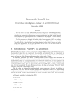
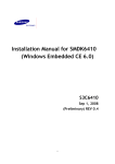
A typical Flash memory device contains many erase blocks. For example, a 4MB Flash
chip might contain 64 erase blocks of 64KB each. Flash memory is also available
with nonuniform erase block sizes, to facilitate flexible data-storage layout. These
are commonly referred to as boot block or boot sector Flash chips. Often the
bootloader is stored in the smaller blocks, and the kernel and other required data
are stored in the larger blocks. Figure 2-3 illustrates the block size layout for a
typical top boot Flash.
Figure 2-3. Boot block flash architecture
To modify data stored in a Flash memory array, the block in which the modified
data resides must be completely erased. Even if only 1 byte in a block needs to be
changed, the entire block must be erased and rewritten.
[6]
Flash block sizes are
relatively large, compared to traditional hard-drive sector sizes. In comparison, a
typical high-performance hard drive has writable sectors of 512 or 1024 bytes. The
ramifications of this might be obvious: Write times for updating data in Flash
memory can be many times that of a hard drive, due in part to the relatively large
quantity of data that must be written back to the Flash for each update. These
write cycles can take several seconds, in the worst case.
[6]
Remember, you can change a 1 to a 0 a byte at a time, but you must erase the
entire block to change any bit from a 0 back to a 1.
Another limitation of Flash memory that must be considered is Flash memory cell
write lifetime. A Flash memory cell has a limited number of write cycles before
failure. Although the number of cycles is fairly large (100K cycles typical per
block), it is easy to imagine a poorly designed Flash storage algorithm (or even a
bug) that can quickly destroy Flash devices. It goes without saying that you should
avoid configuring your system loggers to output to a Flash-based device.
2.3.2. NAND Flash
NAND Flash is a relatively new Flash technology. When NAND Flash hit the market,
traditional Flash memory such as that described in the previous section was
referred to as NOR Flash. These distinctions relate to the internal Flash memory
cell architecture. NAND Flash devices improve upon some of the limitations of
traditional (NOR) Flash by offering smaller block sizes, resulting in faster and
more efficient writes and generally more efficient use of the Flash array.
NOR Flash devices interface to the microprocessor in a fashion similar to many
microprocessor peripherals. That is, they have a parallel data and address bus that
are connected directly
[7]
to the microprocessor data/address bus. Each byte or word
in the Flash array can be individually addressed in a random fashion. In contrast,
NAND devices are accessed serially through a complex interface that varies among
vendors. NAND devices present an operational model more similar to that of a
traditional hard drive and associated controller. Data is accessed in serial bursts,
which are far smaller than NOR Flash block size. Write cycle lifetime for NAND
Flash is an order of magnitude greater than for NOR Flash, although erase times
are significantly smaller.
[7]
Directly in the logical sense. The actual circuitry may contain bus buffers or
bridge devices, etc.
In summary, NOR Flash can be directly accessed by the microprocessor, and code can
even be executed directly out of NOR Flash (though, for performance reasons, this is
rarely done, and then only on systems in which resources are extremely scarce). In
fact, many processors cannot cache instruction accesses to Flash like they can with
DRAM. This further impacts execution speed. In contrast, NAND Flash is more suitable
for bulk storage in file system format than raw binary executable code and data
storage.
2.3.3. Flash Usage
An embedded system designer has many options in the layout and use of Flash
memory. In the simplest of systems, in which resources are not overly constrained,
raw binary data (perhaps compressed) can be stored on the Flash device. When booted,
a file system image stored in Flash is read into a Linux ramdisk block device,
mounted as a file system and accessed only from RAM. This is often a good design
choice when the data in Flash rarely needs to be updated, and any data that does
need to be updated is relatively small compared to the size of the ramdisk. It is
important to realize that any changes to files in the ramdisk are lost upon reboot
or power cycle.
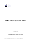
Figure 2-4 illustrates a common Flash memory organization that is typical of a
simple embedded system in which nonvolatile storage requirements of dynamic data
are small and infrequent.
Figure 2-4. Example Flash memory layout
The bootloader is often placed in the top or bottom of the Flash memory array.
Following the bootloader, space is allocated for the Linux kernel image and the
ramdisk file system image,
[8]
which holds the root file system. Typically, the Linux
kernel and ramdisk file system images are compressed, and the bootloader handles
the decompression task during the boot cycle.
[8]
We discuss ramdisk file systems in much detail in Chapter 9, "File Systems."
For dynamic data that needs to be saved between reboots and power cycles, another
small area of Flash can be dedicated, or another type of nonvolatile storage
[9]
can
be used. This is a typical configuration for embedded systems with requirements to
store configuration data, as might be found in a wireless access point aimed at the
consumer market, for example.
[9]
Real-time clock modules often contain small amounts of nonvolatile storage, and
Serial EEPROMs are another common choice for nonvolatile storage of small amounts
of data.
2.3.4. Flash File Systems
The limitations of the simple Flash layout scheme described in the previous
paragraphs can be overcome by using a Flash file system to manage data on the
Flash device in a manner similar to how data is organized on a hard drive. Early
implementations of file systems for Flash devices consisted of a simple block
device layer that emulated the 512-byte sector layout of a common hard drive. These
simple emulation layers allowed access to data in file format rather than
unformatted bulk storage, but they had some performance limitations.
One of the first enhancements to Flash file systems was the incorporation of wear
leveling. As discussed earlier, Flash blocks are subject to a finite write lifetime.
Wear-leveling algorithms are used to distribute writes evenly over the physical
erase blocks of the Flash memory.
Another limitation that arises from the Flash architecture is the risk of data loss
during a power failure or premature shutdown. Consider that the Flash block sizes
are relatively large and that average file sizes being written are often much
smaller relative to the block size. You learned previously that Flash blocks must
be written one block at a time. Therefore, to write a small 8KB file, you must
erase and rewrite an entire Flash block, perhaps 64KB or 128KB in size; in the
worst case, this can take tens of seconds to complete. This opens a significant
window of risk of data loss due to power failure.
One of the more popular Flash file systems in use today is JFFS2, or Journaling
Flash File System 2. It has several important features aimed at improving overall
performance, increasing Flash lifetime, and reducing the risk of data loss in case
of power failure. The more significant improvements in the latest JFFS2 file system
include improved wear leveling, compression and decompression to squeeze more data
into a given Flash size, and support for Linux hard links. We cover this in detail
in Chapter 9, "File Systems," and again in Chapter 10, "MTD Subsystem," when we
discuss the Memory Technology Device (MTD) subsystem.
2.3.5. Memory Space
Virtually all legacy embedded operating systems view and manage system memory as a
single large, flat address space. That is, a microprocessor's address space exists
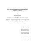
from 0 to the top of its physical address range. For example, if a microprocessor
had 24 physical address lines, its top of memory would be 16MB. Therefore, its
hexadecimal address would range from 0x00000000 to 0x00ffffff. Hardware designs
commonly place DRAM starting at the bottom of the range, and Flash memory from
the top down. Unused address ranges between the top of DRAM and bottom of FLASH
would be allocated for addressing of various peripheral chips on the board. This
design approach is often dictated by the choice of microprocessor. Figure 2-5 is an
example of a typical memory layout for a simple embedded system.
Figure 2-5. Typical embedded system memory map
In traditional embedded systems based on legacy operating systems, the OS and all
the tasks
[10]
had equal access rights to all resources in the system. A bug in one
process could wipe out memory contents anywhere in the system, whether it belonged
to itself, the OS, another task, or even a hardware register somewhere in the
address space. Although this approach had simplicity as its most valuable
characteristic, it led to bugs that could be difficult to diagnose.
[10]
In this discussion, the word task is used to denote any thread of execution,
regardless of the mechanism used to spawn, manage, or schedule it.
High-performance microprocessors contain complex hardware engines called Memory
Management Units (MMUs) whose purpose is to enable an operating system to exercise
a high degree of management and control over its address space and the address
space it allocates to processes. This control comes in two primary forms: access
rights and memory translation. Access rights allow an operating system to assign
specific memory-access privileges to specific tasks. Memory translation allows an
operating system to virtualize its address space, which has many benefits.
The Linux kernel takes advantage of these hardware MMUs to create a virtual
memory operating system. One of the biggest benefits of virtual memory is that it
can make more efficient use of physical memory by presenting the appearance that
the system has more memory than is physically present. The other benefit is that
the kernel can enforce access rights to each range of system memory that it
allocates to a task or process, to prevent one process from errantly accessing
memory or other resources that belong to another process or to the kernel itself.
Let's look at some details of how this works. A tutorial on the complexities of
virtual memory systems is beyond the scope of this book.
[11]
Instead, we examine the
ramifications of a virtual memory system as it appears to an embedded systems
developer.
[11]
Many good books cover the details of virtual memory systems. See Section 2.5.1,
"Suggestions for Additional Reading," at the end of this chapter, for
recommendations.
2.3.6. Execution Contexts
One of the very first chores that Linux performs when it begins to run is to
configure the hardware memory management unit (MMU) on the processor and the data
structures used to support it, and to enable address translation. When this step is
complete, the kernel runs in its own virtual memory space. The virtual kernel
address selected by the kernel developers in recent versions defaults to 0xC0000000.
In most architectures, this is a configurable parameter.
[12]
If we were to look at the
kernel's symbol table, we would find kernel symbols linked at an address starting
with 0xC0xxxxxx. As a result, any time the kernel is executing code in kernel space,
the instruction pointer of the processor will contain values in this range.
[12]
However, there is seldom a good reason to change it.
In Linux, we refer to two distinctly separate operational contexts, based on the
environment in which a given thread
[13]
is executing. Threads executing entirely
within the kernel are said to be operating in kernel context, while application
programs are said to operate in user space context. A user space process can access
only memory it owns, and uses kernel system calls to access privileged resources
such as file and device I/O. An example might make this more clear.
[13]
The term thread here is used in the generic sense to indicate any sequential
flow of instructions.
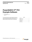
Consider an application that opens a file and issues a read request (see Figure
2-6). The read function call begins in user space, in the C library read() function.
The C library then issues a read request to the kernel. The read request results in
a context switch from the user's program to the kernel, to service the request for
the file's data. Inside the kernel, the read request results in a hard-drive access
requesting the sectors containing the file's data.
Figure 2-6. Simple file read request
Usually the hard-drive read is issued asynchronously to the hardware itself. That
is, the request is posted to the hardware, and when the data is ready, the hardware
interrupts the processor. The application program waiting for the data is blocked
on a wait queue until the data is available. Later, when the hard disk has the data
ready, it posts a hardware interrupt. (This description is intentionally simplified
for the purposes of this illustration.) When the kernel receives the hardware
interrupt, it suspends whatever process was executing and proceeds to read the
waiting data from the drive. This is an example of a thread of execution operating
in kernel context.
To summarize this discussion, we have identified two general execution contexts,
user space and kernel space. When an application program executes a system call
that results in a context switch and enters the kernel, it is executing kernel code
on behalf of a process. You will often hear this referred to as process context
within the kernel. In contrast, the interrupt service routine (ISR) handling the IDE
drive (or any other ISR, for that matter) is kernel code that is not executing on
behalf of any particular process. Several limitations exist in this operational
context, including the limitation that the ISR cannot block (sleep) or call any
kernel functions that might result in blocking. For further reading on these
concepts, consult Section 2.5.1, "Suggestions for Additional Reading," at the end of
this chapter.
2.3.7. Process Virtual Memory
When a process is spawnedfor example, when the user types ls at the Linux command
promptthe kernel allocates memory for the process and assigns a range of virtualmemory addresses to the process. The resulting address values bear no fixed
relationship to those in the kernel, nor to any other running process. Furthermore,
there is no direct correlation between the physical memory addresses on the board
and the virtual memory as seen by the process. In fact, it is not uncommon for a
process to occupy multiple different physical addresses in main memory during its
lifetime as a result of paging and swapping.
Listing 2-4 is the venerable "Hello World," as modified to illustrate the previous
concepts. The goal with this example is to illustrate the address space that the
kernel assigns to the process. This code was compiled and run on the AMCC Yosemite
board, described earlier in this chapter. The board contains 256MB of DRAM memory.
Listing 2-4. Hello World, Embedded Style
#include <stdio.h>
int bss_var;
/* Uninitialized global variable */
int data_var = 1;
/* Initialized global variable */
int main(int argc, char **argv)
{
void *stack_var;
/* Local variable on the stack */
stack_var = (void *)main;
/* Don't let the compiler */
/* optimize it out */
printf("Hello, World! Main is executing at %p\n", stack_var);
printf("This address (%p) is in our stack frame\n", &stack_var);
/* bss section contains uninitialized data */
printf("This address (%p) is in our bss section\n", &bss_var);
/* data section contains initializated data */
printf("This address (%p) is in our data section\n", &data_var);
return 0;
}
Listing 2-5 shows the console output that this program produces. Notice that the
process called hello thinks it is executing somewhere in high RAM just above the
256MB boundary (0x10000418). Notice also that the stack address is roughly halfway
into a 32-bit address space, well beyond our 256MB of RAM (0x7ff8ebb0). How can
this be? DRAM is usually contiguous in systems like these. To the casual observer,
it appears that we have nearly 2GB of DRAM available for our use. These virtual
addresses were assigned by the kernel and are backed by physical RAM somewhere
within the 256MB range of available memory on the Yosemite board.
Listing 2-5. Hello Output
root@amcc:~# ./hello
Hello, World! Main is executing at 0x10000418
This address (0x7ff8ebb0) is in our stack frame
This address (0x10010a1c) is in our bss section
This address (0x10010a18) is in our data section
root@amcc:~#
One of the characteristics of a virtual memory system is that when available
physical RAM goes below a designated threshold, the kernel can swap memory pages
out to a bulk storage medium, usually a hard disk drive. The kernel examines its
active memory regions, determines which areas in memory have been least recently
used, and swaps these memory regions out to disk, to free them up for the current
process. Developers of embedded systems often disable swapping on embedded systems
because of performance or resource constraints. For example, it would be ridiculous
in most cases to use a relatively slow Flash memory device with limited write life
cycles as a swap device. Without a swap device, you must carefully design your
applications to exist within the limitations of your available physical memory.
2.3.8. Cross-Development Environment
Before we can develop applications and device drivers for an embedded system, we
need a set of tools (compiler, utilities, and so on) that will generate binary
executables in the proper format for the target system. Consider a simple
application written on your desktop PC, such as the traditional "Hello World"
example. After you have created the source code on your desktop, you invoke the
compiler that came with your desktop system (or that you purchased and installed)
to generate a binary executable image. That image file is properly formatted to
execute on the machine on which it was compiled. This is referred to as native
compilation. That is, using compilers on your desktop system, you generate code that
will execute on that desktop system.
Note that native does not imply an architecture. Indeed, if you have a toolchain
that runs on your target board, you can natively compile applications for your
target's architecture. In fact, one great way to test a new kernel and custom board
is to repeatedly compile the Linux kernel on it.
Developing software in a cross-development environment requires that the compiler
running on your development host output a binary executable that is incompatible
with the desktop development workstation on which it was compiled. The primary
reason these tools exist is that it is often impractical or impossible to develop
and compile software natively on the embedded system because of resource (typically
memory and CPU horsepower) constraints.
Numerous hidden traps to this approach often catch the unwary newcomer to embedded
development. When a given program is compiled, the compiler often knows how to find
include files, and where to find libraries that might be required for the
compilation to succeed. To illustrate these concepts, let's look again at the "Hello
World" program. The example reproduced in Listing 2-4 above was compiled with the
following command line:
gcc -Wall -o hello hello.c
From Listing 2-4, we see an include the file stdio.h. This file does not reside in
the same directory as the hello.c file specified on the gcc command line. So how
does the compiler find them? Also, the printf() function is not defined in the file
hello.c. Therefore, when hello.c is compiled, it will contain an unresolved reference
for this symbol. How does the linker resolve this reference at link time?
Compilers have built-in defaults for locating include files. When the reference to
the include file is encountered, the compiler searches its default list of locations
to locate the file. A similar process exists for the linker to resolve the reference
to the external symbol printf(). The linker knows by default to search the C
library (libc-*) for unresolved references. Again, this default behavior is built
into the toolchain.
Now consider that you are building an application targeting a PowerPC embedded
system. Obviously, you will need a cross-compiler to generate binary executables
compatible with the PowerPC processor architecture. If you issue a similar
compilation command using your cross-compiler to compile the hello.c example above,
it is possible that your binary executable could end up being accidentally linked
with an x86 version of the C library on your development system, attempting to
resolve the reference to printf(). Of course, the results of running this bogus
hybrid executable, containing a mix of PowerPC and x86 binary instructions
[14]
are
predictable: crash!
[14]
In fact, it wouldn't even compile or link, much less run.
The solution to this predicament is to instruct the cross-compiler to look in
nonstandard locations to pick up the header files and target specific libraries. We
cover this topic in much more detail in Chapter 12, "Embedded Development
Environment." The intent of this example was to illustrate the differences between
a native development environment, and a development environment targeted at crosscompilation for embedded systems. This is but one of the complexities of a crossdevelopment environment. The same issue and solutions apply to cross-debugging, as
you will see starting in Chapter 14, "Kernel Debugging Techniques." A proper crossdevelopment environment is crucial to your success and involves much more than just
compilers, as we shall soon see in Chapter 12, "Embedded Development Environment."
2.4. Embedded Linux Distributions
What exactly is a distribution anyway? After the Linux kernel boots, it expects to
find and mount a root file system. When a suitable root file system has been
mounted, startup scripts launch a number of programs and utilities that the system
requires. These programs often invoke other programs to do specific tasks, such as
spawn a login shell, initialize network interfaces, and launch a user's applications.
Each of these programs has specific requirements of the system. Most Linux
application programs depend on one or more system libraries. Other programs require
configuration and log files, and so on. In summary, even a small embedded Linux
system needs many dozens of files populated in an appropriate directory structure
on a root file system.
Full-blown desktop systems have many thousands of files on the root file system.
These files come from packages that are usually grouped by functionality. The
packages are typically installed and managed using a package manager. Red Hat's
Package Manager (rpm) is a popular example and is widely used for installing,
removing, and updating packages on a Linux system. If your Linux workstation is
based on Red Hat, including the Fedora Core series, typing rpm -qa at a command
prompt lists all the packages installed on your system.
A package can consist of many files; indeed, some packages contain hundreds of
files. A complete Linux distribution can contain hundreds or even thousands of
packages. These are some examples of packages that you might find on an embedded
Linux distribution, and their purpose:
•
initscripts Contains basic system startup and shutdown scripts.
•
apache Implements the popular Apache web server.
•
telnet-server Contains files necessary to implement telnet server
functionality, which allows you to establish Telnet sessions to your embedded
target.
•
glibc Standard C library
•
busybox Compact versions of dozens of popular command line utilities commonly
found on UNIX/Linux systems.
[15]
[15]
This package is important enough to warrant its own chapter. Chapter 11,
"BusyBox," covers BusyBox in detail.
This is the purpose of a Linux distribution as the term has come to be used. A
typical Linux distribution comes with several CD-ROMs full of useful programs,
libraries, tools, utilities, and documentation. Installation of a distribution
typically leaves the user with a fully functional system based on a reasonable set
of default configuration options, which can be tailored to suit a particular set of
requirements. You may be familiar with one of the popular desktop Linux
distributions, such as RedHat or Suse.
A Linux distribution for embedded targets differs in several significant ways.
First, the executable target binaries from an embedded distribution will not run on
your PC, but are targeted to the architecture and processor of your embedded
system. (Of course, if your embedded Linux distribution targets the x86 architecture,
this statement does not apply.) A desktop Linux distribution tends to have many GUI
tools aimed at the typical desktop user, such as fancy graphical clocks,
calculators, personal time-management tools, email clients and more. An embedded
Linux distribution typically omits these components in favor of specialized tools
aimed at developers, such as memory analysis tools, remote debug facilities, and
many more.
Another significant difference between desktop and embedded Linux distributions is
that an embedded distribution typically contains cross-tools, as opposed to native
tools. For example, the gcc toolchain that ships with an embedded Linux distribution
runs on your x86 desktop PC, but produces binary code that runs on your target
system. Many of the other tools in the toolchain are similarly configured: They run
on the development host (usually an x86 PC) but operate on foreign architectures
such as ARM or PowerPC.
2.4.1. Commercial Linux Distributions
There are several vendors of commercial embedded Linux distributions. The leading
embedded Linux vendors have been shipping embedded Linux distributions for some
years. Linuxdevices.com, a popular embedded Linux news and information portal, has
compiled a comprehensive list of commercially available embedded Linux
distributions. It is somewhat dated but is still a very useful starting point. You
can find their compilation at www.linuxdevices.com/articles/AT9952405558.html.
2.4.2. Do-It-Yourself Linux Distributions
You can choose to assemble all the components you need for your embedded project
on your own. You will have to decide whether the risks are worth the effort. If you
find yourself involved with embedded Linux purely for the pleasure of it, such as
for a hobby or college project, this approach might be a good one. However, plan to
spend a significant amount of time assembling all the tools and utilities your
project needs, and making sure they all interoperate together.
For starters, you will need a toolchain. Gcc and binutils are available from
www.fsf.org and other mirrors around the world. Both are required to compile the
kernel and user-space applications for your project. These are distributed
primarily in source code form, and you must compile the tools to suit your
particular cross-development environment. Patches are often required to the most
recent "stable" source trees of these utilities, especially when they will be used
beyond the x86/IA32 architecture. The patches can usually be found at the same
location as the base packages. The challenge is to discover which patch you need
for your particular problem and/or architecture.
2.5. Chapter Summary
This chapter covered many subjects in a broad-brush fashion. Now you have a proper
perspective for the material to follow in subsequent chapters. In later chapters,
this perspective will be expanded to develop the skills and knowledge required to
be successful in your next embedded project.
•
Embedded systems share some common attributes. Often resources are limited,
and user interfaces are simple or nonexistent, and are often designed for a
specific purpose.
•
The bootloader is a critical component of a typical embedded system. If your
embedded system is based on a custom-designed board, you must provide a
bootloader as part of your design. Often this is just a porting effort of an
existing bootloader.
•
Several software components are required to boot a custom board, including
the bootloader and the kernel and file system image.
•
Flash memory is widely used as a storage medium in embedded Linux systems. We
introduced the concept of Flash memory and expand on this coverage in
Chapters 9 and 10.
•
An application program, also called a process, lives in its own virtual memory
space assigned by the kernel. Application programs are said to run in user
space.
•
A properly equipped and configured cross-development environment is crucial
to the embedded developer. We devote an entire chapter to this important
subject in Chapter 12.
•
You need an embedded Linux distribution to begin development of your
embedded target. Embedded distributions contain many components, compiled and
optimized for your chosen architecture.
2.5.1. Suggestions for Additional Reading
Linux Kernel Development, 2nd Edition
Robert Love
Novell Press, 2005
Understanding the Linux Kernel
Daniel P. Bovet & Marco Cesati
O'Reilly & Associates, Inc., 2002
Understanding the Linux Virtual Memory Manager
Bruce Perens
Prentice Hall, 2004
Chapter 3. Processor Basics
In this chapter
•
Stand-alone Processors page 38
•
Integrated Processors: Systems on Chip page 43
•
Hardware Platforms page 61
•
Chapter Summary page 62
In this chapter, we present some basic information to help you navigate the huge
sea of embedded processor choices. We look at some of the processors on the market
and the types of features they contain. Stand-alone processors are highlighted
first. These tend to be the most powerful processors and require external chipsets
to form complete systems. Next we present some of the many integrated processors
that are supported under Linux. Finally, we look at some of the common hardware
platforms in use today.
Literally dozens of embedded processors are available to choose from in a given
embedded design. For the purposes of this chapter, we limit the available discussion
to those that contain a hardware memory-management unit and, of course, to those
that are supported under Linux. One of the fundamental architectural design aspects
of Linux is that it is a virtual memory operating system.
[1]
Employing Linux on a
processor that does not contain an MMU gives up one of the more valuable
architectural features of the kernel and is beyond the scope of this book.
[1]
Linux has support for some basic processors that do not contain MMUs, but this
is not considered a mainstream use of Linux.
3.1. Stand-alone Processors
Stand-alone processors refer to processor chips that are dedicated solely to the
processing function. As opposed to integrated processors, stand-alone processors
require additional support circuitry for their basic operation. In many cases, this
means a chipset or custom logic surrounding the processor to handle functions such
as DRAM controller, system bus addressing configuration, and external peripheral
devices such as keyboard controllers and serial ports. Stand-alone processors often
offer the highest overall CPU performance.
Numerous processors exist in both 32-bit and 64-bit implementations
[2]
that have
seen widespread use in embedded systems. These include the IBM PowerPC 970FX, the
Intel Pentium M, and the Freescale MPC74xx Host Processors, among others.
[2]
32-bit and 64-bit refer to the native width of the processor's main facilities,
such as its execution units, register file and address bus.
Here we present a sample from each of the major manufactures of stand-alone
processors. These processors are well supported under Linux and have been used in
many embedded Linux designs.
3.1.1. IBM 970FX
The IBM 970FX processor core is a high-performance 64-bit capable stand-alone
processor. The 970FX is a superscalar architecture. This means the core is capable
of fetching, issuing, and obtaining results from more than one instruction at a
time. This is done through a pipelining architecture, which provides the effect of
multiple streams of instruction simultaneously. The IBM 970FX contains up to 25
stages of pipelining, depending on the instruction stream and operations contained
therein.
Some of the key features of the 970FX are as follows:
•
A 64-bit implementation of the popular PowerPC architecture
•
Deeply pipelined design, for very-high-performance computing applications
•
Static and dynamic power-management features
•
Multiple sleep modes, to minimize power requirements and maximize battery
life
•
Dynamically adjustable clock rates, supporting lower-power modes
•
Optimized for high-performance, low-latency storage management
The IBM 970FX has been incorporated into a number of high-end server blades and
computing platforms, including IBM's own Blade Server platform.
3.1.2. Intel Pentium M
Certainly one of the most popular architectures, x86 in both 32- and 64-bit
flavors (more properly called IA32 and IA64, respectively) has been employed for
embedded devices in a variety of applications. In the most common form, these
platforms are based on a variety of commercial off-the-shelf (COTS) hardware
implementations. Numerous manufacturers supply x86 single-board computers and
complete platforms in a variety of form factors. See Section 3.2, "Integrated
Processors: Systems on Chip," later in this chapter for a discussion of the more
common platforms in use today.
The Intel Pentium M has been used in a wide variety of laptop computers and has
found a niche in embedded products. Like the IBM 970FX processor, the Pentium M is
a superscalar architecture. These characteristics make it attractive in embedded
applications:
•
The Pentium M is based on the popular x86 architecture, and thus is widely
supported by a large ecosystem of hardware and software vendors.
•
It consumes less power than other x86 processors.
•
Advanced power-management features enable low-power operating modes and
multiple sleep modes.
•
Dynamic clock speed capability enhances battery-powered operations such as
standby.
•
On chip thermal monitoring enables automatic transition to lower power modes,
to reduce power consumption in overtemperature conditions.
•
Multiple frequency and voltage operating points (dynamically selectable) are
designed to maximize battery life in portable equipment.
Many of these features are especially useful for embedded applications. It is not
uncommon for embedded products to require portable or battery-powered
configurations. The Pentium M has enjoyed popularity in this application space
because of its power- and thermal-management features.
3.1.3. Freescale MPC7448
The Freescale MPC7448 contains what is referred to as a fourth-generation PowerPC
[3]
core, commonly called G4.
This high-performance 32-bit processor is commonly found
in networking and telecommunications applications. Several companies manufacture
blades that conform to an industry-standard platform specification, including this
and other similar stand-alone Freescale processors. We examine these platforms in
Section 3.3, "Hardware Platforms," later in this chapter.
[3]
Freescale literature now refers to the G4 core as the e600 core.
The MPC7448 has enjoyed popularity in a wide variety of signal-processing and
networking applications because of the advanced feature set highlighted here:
•
Operating clock rates in excess of 1.5GHz
•
1MB onboard L2 cache
•
Advanced power-management capabilities, including multiple sleep modes
•
Advanced AltiVec vector-execution unit
•
Voltage scaling for reduced-power configurations
The MPC7448 contains a Freescale technology called AltiVec to enable very fast
algorithmic computations and other data-crunching applications. The AltiVec unit
consists of a register file containing 32 very wide (128-bit) registers. Each value
within one of these AltiVec registers can be considered a vector of multiple
elements. AltiVec defines a set of instructions to manipulate this vector data
effectively in parallel with core CPU instruction processing. AltiVec operations
include such computations as sum-across, multiply-sum, simultaneous data distribute
(store), and data gather (load) instructions.
Programmers have used the AltiVec hardware to enable very fast software
computations commonly found in signal-processing and network elements. Examples
include fast Fourier Transform, digital signal processing such as filtering, MPEG
video coding and encoding, and fast generation of encryption protocols such as DES,
MD5, and SHA1.
Other chips in the Freescale lineup of stand-alone processors include the MPC7410,
MPC7445, MPC7447, MPC745x, and MPC7xx family.
3.1.4. Companion Chipsets
Stand-alone processors such as those just described require support logic to
connect to and enable external peripheral devices such as main system memory
(DRAM), ROM or Flash memory, system busses such as PCI, and other peripherals, such
as keyboard controllers, serial ports, IDE interfaces, and the like. This support
logic is often accomplished by companion chipsets, which may even be purposedesigned specifically for a family of processors.
For example, the Pentium M is supported by one such chipset, called the 855GM. The
855GM chipset is the primary interface to graphics and memorythus, the suffix-GM.
The 855GM has been optimized as a companion to the Pentium M. Figure 3-1
illustrates the relationship between the processor and chipsets in this type of
hardware design.
Figure 3-1. Processor/chipset relationship
Note the terminology that has become common for describing these chipsets. The
Intel 855GM is an example of what is commonly referred to as a northbridge chip
because it is directly connected to the processor's high-speed front side bus (FSB).
Another companion chip that provides I/O and PCI bus connectivity is similarly
referred to as the southbridge chip because of its position in the architecture. The
southbridge chip (actually, an I/O controller) in these hardware architectures is
responsible for providing interfaces such as those shown in Figure 3-1, including
Ethernet, USB, IDE, audio, keyboard, and mouse controllers.
On the PowerPC side, the Tundra Tsi110 Host Bridge for PowerPC is an example of a
chipset that supports the stand-alone PowerPC processors. The Tsi110 supports
several interface functions for many common stand-alone PowerPC processors. The
Tundra chip supports the Freescale MPC74xx and the IBM PPC 750xx family of
processors. The Tundra chip can be used by these processors to provide direct
interfaces to the following peripherals:
•
DDR DRAM, integrated memory controller
•
Ethernet (the Tundra provides four gigabit Ethernet ports)
•
PCI Express (supports 2 PCI Express ports)
•
PCI/X (PCI 2.3, PCI-X, and Compact PCI [cPCI])
•
Serial ports
•
I2C
•
Programmable interrupt controller
•
Parallel port
Many manufacturers of chipsets exist, including VIA Technologies, Marvell, Tundra,
nVidia, Intel, and others. Marvell and Tundra primarily serve the PowerPC market,
whereas the others specialize in Intel architectures. Hardware designs based on one
of the many stand-alone processors, such as Intel x86, IBM, or Freescale PowerPC,
need to have a companion chipset to interface to system devices.
One of the advantages of Linux as an embedded OS is rapid support of new chipsets.
Linux currently has support for those chipsets mentioned here, as well as many
others. Consult the Linux source code and configuration utility for information on
your chosen chipset.
3.2. Integrated Processors: Systems on Chip
In the previous section, we highlighted stand-alone processors. Although they are
used for many applications, including some high-horsepower processing engines, the
vast majority of embedded systems employ some type of integrated processor, or
system on chip (SOC). Literally scores, if not hundreds, exist to choose from. We
examine a few from the industry leaders and look at some of the features that set
each group apart. As in the section on stand-alone processors, we focus only on
those integrated processors with strong Linux support.
Several major processor architectures exist, and each architecture has examples of
integrated SOCs. PowerPC has been a traditional leader in many networking- and
telecommunications-related embedded applications, while MIPS might have the market
lead in lower-end consumer-grade equipment.
[4]
ARM is used in many cellular phones.
These represent the major architectures in widespread use in embedded Linux
systems. However, as you will see in Chapter 4, "The Linux Kernel: A Different
Perspective," Linux supports more than 20 different hardware architectures today.
[4]
These are the author's own opinions based on market observation and not based on
any scientific data.
3.2.1. PowerPC
PowerPC is a Reduced Instruction Set Computer (RISC) architecture jointly designed
by engineers from Apple, IBM, and Motorola's semiconductor division (now an
independent entity spun off as Freescale Semiconductor). Many good documents
describe the PowerPC architecture in great detail. Consult the "Suggestions for
Additional Reading" at the end of this chapter as a starting point.
PowerPC processors have found their way into embedded products of every
description. From automotive, consumer, and networking applications to the largest
data and telecommunications switches, PowerPC is one of the most popular
architectures for embedded applications. Because of this popularity, there exists a
large array of hardware and software solutions from numerous manufacturers
targeted at PowerPC.
3.2.2. AMCC PowerPC
Some of the examples later in this book are based on the AMCC PowerPC 440EP
Embedded Processor. The 440EP is a popular integrated processor found in many
networking and communications products. The following list highlights some of the
features of the 440EP:
•
On-chip dual-data-rate (DDR) SDRAM controller
•
Integrated NAND Flash controller
•
PCI bus interface
•
Dual 10/100Mbps Ethernet ports
•
On-chip USB 2.0 interface
•
Up to four user-configurable serial ports
•
Dual I C controllers
•
Programmable Interrupt Controller
•
Serial Peripheral Interface (SPI) controller
•
Programmable timers
•
JTAG interface for debugging
2
This is indeed a complete system on chip (SOC). Figure 3-2 is a block diagram of
the AMCC PowerPC 440EP Embedded Processor. With the addition of memory chips and
physical I/O hardware, a complete high-end embedded system can be built around this
integrated microprocessor with minimal interface circuitry required.
Figure 3-2. AMCC PPC 440EP Embedded Processor (Courtesy AMCC Corporation)
[View full size image]
Many manufacturers offer reference hardware platforms to enable a developer to
explore the capabilities of the processor or other hardware. The examples later in
this book (Chapters 14, "Kernel Debugging Techniques"; and 15, "Debugging Embedded
Linux Applications") were executed on the AMCC Yosemite board, which is the
company's reference platform containing the 440EP shown in Figure 3-2.
Numerous product configurations are available with PowerPC processors. As
demonstrated in Figure 3-2, the AMCC 440EP contains sufficient I/O interfaces for
many common products, with very little additional circuitry. Because this processor
contains an integrated floating-point unit (FPU), it is ideally suited for products
such as network-attached imaging systems, general industrial control, and
networking equipment.
AMCC's PowerPC product lineup includes several configurations powered by two proven
cores. Their 405 core products are available in configurations with and without
Ethernet controllers. All 405 core configurations include integrated SDRAM
2
controllers, dual UARTs for serial ports, I C for low-level onboard management
communications, general-purpose I/O pins, and integral timers. The AMCC 405 core
integrated processors provide economical performance on a proven core for a wide
range of applications that do not require a hardware FPU.
The AMCC 440-based core products raise the performance level and add peripherals.
The 440EP featured in some of our examples includes a hardware FPU. The 440GX adds
two triple-speed 10/100/1000MB Ethernet interfaces (in addition to the two
10/100Mbps Ethernet ports) and TCP/IP hardware acceleration for high-performance
networking applications. The 440SP adds hardware acceleration for RAID 5/6
applications. All these processors have mature Linux support. Table 3-1 summarizes
the highlights of the AMCC 405xx family.
Table 3-1. AMCC PowerPC 405xx Highlights Summary
Feature
405CR
405EP
405GP
405GPr
PowerPC
PowerPC
PowerPC
PowerPC
405
405
405
405
133-266MHz
133-333MHz
133-266MHz
266-400MHz
DRAM controller
SDRAM/133
SDRAM/133
SDRAM/133
SDRAM/133
Ethernet 10/100
N
2
1
1
GPIO lines
23
32
24
24
UARTs
2
2
2
2
4 channel
4 channel
4 channel
4 channel
I C controller
Y
Y
Y
Y
PCI host controller
N
Y
Y
Y
Interrupt controller
Y
Y
Y
Y
Core/speeds
DMA controller
2
See the AMCC website, at www.amcc.com/embedded, for complete details.
Table 3-2 summarizes the features of the AMCC 440xx family of processors.
Table 3-2. AMCC PowerPC 440xx Highlights Summary
Feature
Core/speeds
440EP
440GP
440GX
440SP
PowerPC
PowerPC
PowerPC
PowerPC
440
440
440
440
333-667MHz 400-500MHz 533-800MHz 533-667MHz
DRAM controller
DDR
DDR
DDR
DDR
Ethernet 10/100
2
2
2
via GigE
Gigabit Ethernet
N
N
2
1
GPIO lines
64
32
32
32
UARTs
4
2
2
3
4 channel
4 channel
4 channel
3 channel
DMA controller
Table 3-2. AMCC PowerPC 440xx Highlights Summary
Feature
440EP
440GP
440GX
440SP
I C controller
2
2
2
2
PCI host controller
Y
PCI-X
PCI-X
three PCI-
2
X
SPI controller
Y
N
N
N
Interrupt controller
Y
Y
Y
Y
3.2.3. Freescale PowerPC
Freescale Semiconductor has a large range of PowerPC processors with integrated
peripherals. The manufacturer is currently advertising its PowerPC product
portfolio centered on three broad vertical-market segments: networking, automotive,
and industrial. Freescale PowerPC processors have enjoyed enormous success in the
networking market segment. This lineup of processors has wide appeal in a large
variety of network equipment, from the low end to the high end of the product
space.
In a recent press release, Freescale Semiconductor announced that it had shipped
more than 200 million integrated communications processors.
[5]
Part of this success
is based around the company's PowerQUICC product line. The PowerQUICC architecture
has been shipping for more than a decade. It is based on a PowerPC core integrated
with a QUICC engine (also called a communications processor module or CPM in the
Freescale literature). The QUICC engine is an independent RISC processor designed to
offload the communications processing from the main PowerPC core, thus freeing up
the PowerPC core to focus on control and management applications. The QUICC engine
is a complex but highly flexible communications peripheral controller.
[5]
On the Freescale website, navigate to Media Center, Press Releases. This one was
dated 10/31/2005 from Austin, Texas.
In its current incarnation, PowerQUICC encompasses four general families. For
convenience, as we discuss these PowerQUICC products, we refer to it as PQ.
The PQ I family includes the original PowerPC-based PowerQUICC implementations and
consists of the MPC8xx family of processors. These integrated communications
processors operate at 50-133MHz and feature the embedded PowerPC 8xx core. The PQ
I family has been used for ATM and Ethernet edge devices such as routers for the
home and small office (SOHO) market, residential gateways, ASDL and cable modems,
and similar applications.
The CPM or QUICC engine incorporates two unique and powerful communications
controllers. The Serial Communication Controller (SCC) is a flexible serial
interface capable of implementing many serial-based communications protocols,
including Ethernet, HDLC/SDLC, AppleTalk, synchronous and asynchronous UARTs, IrDA,
and other bit stream data.
The Serial Management Controller (SMC) is a module capable of similar serialcommunications protocols, and includes support for ISDN, serial UART, and SPI
protocols.
Using a combination of these SCCs and SMCs, it is possible to create very flexible
I/O combinations. An internal time-division multiplexer even allows these
interfaces to implement channelized communications such as T1 and E1 I/O.
Table 3-3 summarizes a small sampling of the PQ I product line.
Table 3-3. Freescale Select PowerQUICC I Highlights
Feature
MPC850
MPC860
Core/speeds
PowerPC
PowerPC
8xx
8xx
Up to
Up to
Up to
Up to
80MHz
80MHz
133MHz
133MHz
DRAM controller
Y
Y
Y
Y
USB
Y
N
Y
Y
SPI controller
Y
Y
Y
Y
I C controller
Y
Y
Y
Y
SCC controllers
2
4
1
3
SMC controllers
2
2
1
1
Security engine
N
N
Y
Y
Dedicated Fast Ethernet
N
N
2
2
2
controller
MPC875
MPC885
PowerPC 8xx PowerPC 8xx
The next step up in the Freescale PowerPC product line is PowerQUICC II. PQ II
incorporates the company's G2 PowerPC core derived from the 603e embedded PowerPC
core. These integrated communications processors operate at 133-450MHz and feature
multiple 10/100Mbps Ethernet interfaces, security engines, and ATM and PCI support,
among many others. The PQ II encompasses the MPC82xx products.
PQ II adds two new types of controllers to the QUICC engine. The FCC is a fullduplex fast serial communications controller. The FCC supports high-speed
communications such as 100Mbps Ethernet and T3/E3 up to 45Mbps. The MCC is a
multichannel controller capable of 128KB x 64KB channelized data.
Table 3-4 summarizes the highlights of selected PowerQUICC II processors.
Table 3-4. Freescale Select PowerQUICC II Highlights
Feature
Core/speeds
MPC8250
MPC8260
MPC8272
MPC8280
G2/603e
G2/603e
G2/603e
G2/603e
150-200MHz 100-300MHz 266-400MH 266-400MH
DRAM
z
z
Y
Y
Y
Y
USB
N
N
Y
Via SCC4
SPI controller
Y
Y
Y
Y
I C controller
Y
Y
Y
Y
SCC controllers
4
4
3
4
SMC controllers
2
2
2
2
FCC controllers
3
3
2
3
MCC controllers
1
2
0
2
controller
2
Based on the Freescale PowerPC e300 core (evolved from the G2/603e), the PowerQUICC
II Pro family operates at 266-667MHz and features support for Gigabit Ethernet,
dual data rate (DDR) SDRAM controllers, PCI, high-speed USB, security acceleration,
and more. These are the MPC83xx family of processors. The PQ II and PQ II Pro
families of processors have been designed into a wide variety of equipment, such as
LAN and WAN switches, hubs and gateways, PBX systems, and many other systems with
similar complexity and performance requirements.
The PowerQUICC II Pro contains three family members without the QUICC engine, and
two that are based on an updated version of the QUICC engine. The MPC8358E and
MPC8360E both add a new Universal Communications Controller, which supports a
variety of protocols.
Table 3-5 summarizes the highlights of select members of the PQ II Pro family.
Table 3-5. Freescale Select PowerQUICC II Pro Highlights
Feature
Core/speeds
MPC8343E MPC8347E MPC8349E MPC8360E
e300
e300
e300
e300
266-400MH 266-667MH 400-667MH 266-667MH
z
z
z
z
Y-DDR
Y-DDR
Y-DDR
Y-DDR
USB
Y
2
2
Y
SPI controller
Y
Y
Y
Y
I C controller
2
2
2
2
Ethernet 10/100/1000
2
2
2
Via UCC
UART
2
2
2
2
PCI controller
Y
Y
Y
Y
Security engine
Y
Y
Y
Y
MCC
0
0
0
1
UCC
0
0
0
8
DRAM controller
2
At the top of the PowerQUICC family are the PQ III processors. These operate
between 600MHz and 1.5GHz. They are based on the e500 core and support Gigabit
Ethernet, DDR SDRAM, RapidIO, PCI and PCI/X, ATM, HDLC, and more. This family
incorporates the MPC85xx product line. These processors have found their way into
high-end products such as wireless base station controllers, optical edge switches,
central office switches, and similar equipment.
Table 3-6 highlights some of the PQ III family members.
Table 3-6. Freescale Select PowerQUICC III Highlights
Feature
Core/speeds
MPC8540
MPC8548E
MPC8555E
MPC8560
e500
e500
e500
e500
Up to 1.0GHz Up to 1.5GHz Up to 1.0GHz Up to 1.0GHz
DRAM controller
Y-DDR
Y-DDR
Y-DDR
Y-DDR
USB
N
N
Via SCC
N
SPI controller
N
N
Y
Y
I C controller
Y
Y
Y
Y
Ethernet 10/100
1
Via GigE
Via SCC
Via SCC
Gigabit Ethernet
2
4
2
2
UART
2
2
2
Via SCC
PCI/PCI-X
PCI/PCI-X
PCI
PCI/PCI-X
Rapid IO
Y
Y
N
Y
Security engine
N
Y
Y
N
SCC
3
4
FCC
2
3
SMC
2
0
MCC
0
2
2
PCI controller
3.2.4. MIPS
You might be surprised to learn that 32-bit processors based on the MIPS
architecture have been shipping for more than 20 years. The MIPS architecture was
designed in 1981 by a Stanford University engineering team led by Dr. John
Hennessey, who later went on to form MIPS Computer Systems, Inc. That company has
morphed into the present-day MIPS Technologies, whose primary role is the design
and subsequent licensing of MIPS architecture and cores.
The MIPS core has been licensed by many companies, several of which have become
powerhouses in the embedded processor market. MIPS is a Reduced Instruction Set
Computing (RISC) architecture with both 32-bit and 64-bit implementations shipping
in many popular products. MIPS processors are found in a large variety of products,
from high-end to consumer devices. It is public knowledge that MIPS processors
power many popular well-known consumer products, such as Sony high definition
television sets, Linksys wireless access points, and the popular Sony PlayStation 2
[6]
game console.
[6]
Source: www.mips.com/content/PressRoom/PressReleases/2003-12-22
The MIPS Technology website lists 73 licensees who are currently engaged in
manufacturing products using MIPS processor cores. Some of these companies are
household names, as with Sony, Texas Instruments, Cisco's Scientific Atlanta (a
leading manufacturer of cable TV set-top boxes), Motorola, and others. Certainly,
one of the largest and most successful of these is Broadcom Corporation.
3.2.5. Broadcom MIPS
Broadcom is a leading supplier of SOC solutions for markets such as cable TV settop boxes, cable modems, HDTV, wireless networks, Gigabit Ethernet, and Voice over
IP (VoIP). Broadcom's SOCs have been very popular in these markets. We mentioned
earlier that you likely have Linux in your home even if you don't know it. Chances
are, if you do, it is running on a Broadcom MIPS-based SOC.
In 2000, Broadcom acquired SiByte Inc., which resulted in the communications
processor product lineup the company is currently marketing. These processors
currently ship in single-core, dual-core, and quad-core configurations. The company
still refers to them as SiByte processors.
The single-core SiByte processors include the BCM1122 and BCM1125H. They are both
based on the MIPS64 core and operate at clock speeds at 400-900MHz. They include
on-chip peripheral controllers such as DDR SDRAM controller, 10/100Mbps Ethernet,
and PCI host controller. Both include SMBus serial configuration interface, PCMCIA,
and two UARTs for serial port connections. The BCM1125H includes a triple-speed
10/100/1000Mbps Ethernet controller. One of the more striking features of these
processors is their power dissipation. Both feature a 4W operating budget at 400MHz
operation.
The dual-core SiByte processors include the BCM1250, BCM1255, and BCM1280. Also
based on the MIPS64 core, these processors operate at clock rates from 600MHz
(BCM1250) to as high as 1.2GHz (BCM1255 and BCM1280). These dual-core chips include
integrated peripheral controllers such as DDR SDRAM controllers, various
combinations of Gigabit Ethernet controllers, 64-bit PCI-X interfaces, and SMBus,
PCMCIA, and multiple UART interfaces. Like their single-core cousins, these dual-
core implementations also feature low power dissipation. For example, the BCM1255
features a 13W power budget at 1GHz operation.
The quad-core SiByte processors include the BCM1455 and BCM1480 communications
processors. As with the other SiByte processors, these are based on the MIPS64 core.
The cores can be run from 800MHz to 1.2GHz. These SOCs include integrated DDR SDRAM
controllers, four separate Gigabit Ethernet MAC controllers, and 64-bit PCI-X host
controllers, and also contain SMBus, PCMCIA, and four serial UARTs.
Table 3-7 summarizes select Broadcom SiByte processors.
Table 3-7. Broadcom Select SiByte Processor Highlights
Feature
Core/speeds
BCM1125H
BCM1250
BCM1280
BCM1480
SB-1
Dual SB-1
Dual SB-1
Quad SB-1
MIPS64
MIPS64
MIPS64
MIPS64
400-900MH 600-1000MHz 800-1200MHz 800-1200MHz
z
DRAM controller
Y-DDR
Y-DDR
Y-DDR
Y-DDR
Serial interface
2-55Mbps
2-55Mbps
4 UART
4 UART
SMBus interface
2
2
2
2
PCMCIA
Y
Y
Y
Y
Gigabit Ethernet (10/100/1000Mbps)
2
3
4
4
PCI controller
Y
Y
Y PCI/PCI- Y PCI/PCIX
Security engine
N
N
N
High-speed I/O (HyperTransport)
1
1
3
X
3
3.2.6. AMD MIPS
Advanced Micro Devices also plays a significant role in the embedded MIPS
controller market. The company's 2002 acquisition of Alchemy Semiconductor garnered
several popular single-chip integrated SOCs based on the MIPS32 core and
architecture. The Alchemy line from AMD is based on the popular MIPS32 core. All
feature relatively low power dissipation and a high level of onboard system
integration.
The Au1000 and Au1100 operate at clock rates of 266-500MHz. Both feature onboard
SDRAM controllers and separate bus controllers for attachment to external devices
such as Flash and PCMCIA. Table 3-8 summarizes the current Alchemy product line.
Table 3-8. AMD Alchemy MIPS Highlights Summary
Feature
[*]
Au1000
Au1100
Au1200
Au1500
Au1550
MIPS32
MIPS32
MIPS32
MIPS32
MIPS32
266-500MHz
333-500MHz
333-500MH
333-500MHz
333-500MHz
SDRAM
DDR SDRAM
2
2
Core/speeds
z
DRAM
SDRAM
SDRAM
DDR SDRAM
Ethernet 10/100
2
1
GPIO lines
32
48
48
39
43
UARTs
4
3
2
2
3
controller
USB 1.1
Host + device Host + device
AC-97 audio
USB 2.0
1
1
Via SPC
I S controller
1
1
Via SPC
SD/MMC
N
2
2
2
[*]
Host + device Host + device
1
Via SPC
Via SPC
N
N
Other peripherals include IrDA controller, LCD controller, 2 SPCs, Power
management, DMA engine, RTC, Camera interface, LCD controller, h/w hardware
acceleration of encryption/decryption, PCI host controller, 4 SPCs, and Security
engine.
3.2.7. Other MIPS
As we pointed out earlier, nearly 100 current MIPS licensees are shown on the MIPS
Technologies licensees web page, at
www.mips.com/content/Licensees/ProductCatalog/licensees. Unfortunately, it is not
possible in the space provided here to cover them all. Start your search at the
MIPS technologies website for a good cross-section of the MIPS processor vendors.
For example, ATI Technologies uses a MIPS core in its Xilleon set-top box family of
chipsets. Cavium Network's Octeon family uses MIPS64 cores in a variety of multicore
processor implementations. Integrated Device Technology, Inc., (IDT) has a family of
integrated communications processors called Interprise, based on the MIPS
architecture. PMC-Sierra, NEC, Toshiba, and others have integrated processors based
on MIPS. All of these and more are well supported under Linux.
3.2.8. ARM
The ARM architecture has achieved a very large market share in the consumer
electronics marketplace. Many popular and now ubiquitous products contain ARM
cores. Some well-known examples include the Sony PlayStation Portable (PSP), Apple
iPod Nano,
[7]
Nintendo Game Boy Micro and DS, TomTom GO 300 GPS, and the Motorola
E680i Mobile Phone, which features embedded Linux. Processors containing ARM cores
power a majority of the world's digital cellular phones, according to the ARM
Corporate Backgrounder at www.arm.com/miscPDFs/3822.pdf.
[7]
Reported by ARM to be the top-selling toy during the Christmas 2005 shopping
season in the United States.
The ARM architecture is developed by ARM Holdings, plc and licensed to
semiconductor manufacturers around the globe. Many of the world's leading
semiconductor companies have licensed ARM technology and are currently shipping
integrated processors based on one of the several ARM cores.
3.2.9. TI ARM
Texas Instruments uses ARM cores in the OMAP family of integrated processors. These
processors contain many integrated peripherals intended to be used as single-chip
solutions for various consumer products, such as cellular handsets, PDAs, and
similar multimedia platforms. In addition to the interfaces commonly found on
2
integrated processors, such as UARTs and I C, the OMAP devices contain a wide range
of special-purpose interfaces, including the following:
•
LCD screen and backlight controllers
•
Buzzer driver
•
Camera interface
•
MMC/SD card controller
•
Battery-management hardware
•
USB client/host interfaces
•
Radio modem interface logic
•
Integrated 2D or 3D graphics accelerators
•
Integrated security accelerator
•
S-Video outputs
•
IrDA controller
•
DACs for direct TV (PAL/NTSC) video output
•
Integrated DSPs for video and audio processing
Many popular cellular handsets and PDA devices have been marketed based on the TI
OMAP platform. Because they are based on an ARM core, these processors are
supported by Linux today. Table 3-9 compares some of the more recent members of
the TI OMAP family.
Table 3-9. TI ARM OMAP Highlights Summary
Feature
Core/speeds
OMAP1710
OMAP2420
OMAP2430
OMAP3430
ARM926
ARM11
ARM1136
ARM Cortex A8
330MHz
330MHz
550MHz
TEJ
Up to
200MHz
DRAM controller
Y
Y
Y
Y
UARTs
Y
Y
Y
Y
Client +
Client + host
Client + host
Client + host
USB
host
2
I C controller
Y
Y
Y
Y
MMC-SD interface
Y
Y
Y
Y
Keypad controller
Y
Y
Y
Y
Camera interface
Y
Y
Y
Y
Graphics
2D
2D/3D
2D/3D
Y
TM320C55x
TM320C55x
N
N
N
Imaging Video
Imaging Video
Imaging Video
Accelerator
Accelerator (IVA
Accelerator (IVA
(IVA)
2)
2 +)
Y
Y
Y
Y
Y
Y
Y
Y
Y
Y
Y
Y
accelerator
Integrated DSP
Video acceleration
hardware
Security
accelerator
Audio codec
support
Bluetooth & RF
modem support
interface
Table 3-9. TI ARM OMAP Highlights Summary
Feature
OMAP1710
OMAP2420
OMAP2430
OMAP3430
LCD controller
Y
Y
Y
Y
Display controllers
N
PAL/NTSC
PAL/NTSC
PAL/NTSC
VGA/QVGA
VGA/QVGA
QVGA/XGA
3.2.10. Freescale ARM
The success of the ARM architecture is made more evident by the fact that leading
manufacturers of competing architectures have licensed ARM technology. As a prime
example, Freescale Semiconductor has licensed ARM technology for its line of i.MX
application processors. These popular ARM-based integrated processors have achieved
widespread industry success in multimedia consumer devices such as portable game
platforms, PDAs, and cellular handsets.
The Freescale ARM product portfolio includes the i.MX21 and i.MX31 application
processors. The i.MX21 features an ARM9 core, and the i.MX31 has an ARM11 core. Like
their TI counterparts, these SOCs contain many integrated peripherals required by
portable consumer electronics devices with multimedia requirements. The i.MX21/31
contain some of the following integrated interfaces:
•
Graphics accelerator
•
MPEG-4 encoder
•
Keypad and LCD controllers
•
Camera interface
•
Audio multiplexer
•
IrDA infrared I/O
•
SD/MMC interface
•
Numerous external I/O, such as PCMCIA, USB, DRAM controllers, and UARTs for
serial port connection
3.2.11. Intel ARM XScale
Intel manufactures and markets several integrated processors based on the ARM v5TE
architecture. Intel uses the XScale name for the architecture. These products are
grouped into several application categories. Table 3-10 summarizes the XScale
families by application type.
Table 3-10. Intel XScale Processor Summary
Category
Application
Example Processors
Application
Cellular handsets and PDAs
PXA27x, PXA29x
High-speed data processing used in storage,
IOP331/332/333
processors
I/O processors
printing, telematics, and so on
Network
Networking and communications data plane
IXP425, IXP465
processors
processing, fast packet processing, and so on IXP2350, IXP2855
Many consumer and networking products have been developed using Intel XScale
architecture processors. Some well-known examples include the GPS iQue M5 from
Garmin, the iPAQ by Hewlett-Packard, smart phones from Palm (Treo) and Motorola
(A760), and many others. Linux currently supports all these processors.
Intel's network processors are found in high-performance networking equipment where
requirements exist for fast data-path processing. Examples include deep packet
inspection, data encryption/decryption, packet filtering, and signal processing.
These network processors each contain an ARM core coupled with one or more
dedicated processing engines, called a network processing engine (NPE). These NPEs
are dedicated to specific data-path manipulation in real time at wire speeds. The
NPE is a microprocessor, in the sense that it can execute microcoded algorithms in
parallel with the thread of execution in the ARM core. Refer to the Intel website,
at www.intel.com, for additional information on this powerful family of integrated
processors.
3.2.12. Other ARM
More than 100 semiconductor companies are developing integrated solutions based on
ARM technologyfar too many to list here. Many offer specialized application
processors serving vertical markets such as the handset market, storage area
networking, network processing, and the automotive market, as well as many more.
These companies include Altera, PMC-Sierra, Samsung Electronics, Philips
Semiconductor, Fujitsu, and more. See the ARM Technologies website at www.arm.com
for additional ARM licensees and information.
3.2.13. Other Architectures
We have covered the major architectures in widespread use in embedded Linux
systems. However, for completeness, you should be aware of other architectures for
which support exists in Linux. A recent Linux snapshot revealed 25 architecture
branches (subdirectories). In some instances, the 64-bit implementation of an
architecture is separated from its 32-bit counterpart. In other cases, ports are not
current or are no longer maintained.
The Linux source tree contains ports for Sun Sparc and Sparc64, the Xtensa from
Tensilica, and the v850 from NEC, to name a few. Spend a few minutes looking
through the architecture branches of the Linux kernel to see the range of
architectures for which Linux has been ported. Beware, however, that not all these
architectures might be up-to-date in any given snapshot. You can be reasonably
certain that the major architectures are fairly current, but the only way to be
certain is to follow the development in the Linux community or consult with your
favorite embedded Linux vendor. Appendix E, "Open Source Resources," contains a list
of resources you can consult to help you stay current with Linux developments.
3.3. Hardware Platforms
The idea of a common hardware reference platform is not new. The venerable PC/104
and VMEbus are two examples of hardware platforms that have withstood the test of
time in the embedded market.
[8]
More recent successful platforms include CompactPCI
and its derivatives.
[8]
VMEbus isn't really a hardware reference platform, per se, but based on Eurocard
physical standards, the level of compatibility among multiple vendors qualifies it
for the label.
3.3.1. CompactPCI
The CompactPCI (cPCI) hardware platform is based on PCI electrical standards and
Eurocard physical specifications. cPCI has the following general features:
•
Vertical cards of 3U or 6U heights
•
Latch system for securing and ejecting cards
•
Front- or rear-panel I/O connections supported
•
High-density backplane connector
•
Staggered power pins for hot-swap support
•
Support by many vendors
•
Compatibility with standard PCI chipsets
You can view highlights of and obtain specifications for the cPCI architecture at
the PCI Industrial Computer Manufacturers Group (PICMG) cPCI web page, at
www.picmg.org/compactpci.stm.
3.3.2. ATCA
A successor to the successful cPCI, Advanced Telecommunications Computing
Architecture is the name given to the architecture and platforms designed around
the PICMG 3.x series of specifications. Many top-tier hardware manufacturers are
shipping or developing new ATCA-based platforms. The primary applications for ATCA
platforms are carrier-class telecommunications switching and transport equipment,
and high-end data-center server and storage equipment.
ATCA platforms are leading the industry trend away from in-house proprietary
hardware and software platforms. Many of the largest equipment manufacturers in
the telecommunications and networking markets have been slowly moving away from
the custom, in-house-designed hardware platforms. This trend is also evident in the
software platforms, from operating systems to so-called middleware such as highavailability and protocol stack solutions. Downsizing and time-to-market pressures
are two key factors driving this trend.
ATCA is defined by several PICMG specifications. Table 3-11 summarizes these
specifications.
Table 3-11. ATCA PICMG 3.x Specification Summary
Specificati Summary
on
PICMG 3.0
Mechanical specifications, including interconnects, power, cooling, and
base system management
PICMG 3.1
Ethernet and Fiber Channel switching fabric interface
PICMG 3.2
Infiniband switching fabric interface
PICMG 3.3
StarFabric interface
PICMG 3.4
PCI Express interface
PICMG 3.5
RapidIO Interface
The platforms described in this section are the most relevant in any discussion of
embedded Linux platforms today. Especially with ATCA, the industry is increasingly
moving toward commercial off-the-shelf (COTS) technology. Both ATCA and Linux play
increasingly important roles in this industry trend.
3.4. Chapter Summary
•
Many stand-alone processors are supported under Linux. The most widely
supported of these are IA32/IA64 and PowerPC architectures. These stand-alone
processors are used as building blocks to build very-high-performance
computing engines. We presented several examples from Intel, IBM, and
Freescale.
•
Integrated processors, or systems on chip (SOCs), dominate the embedded Linux
landscape. Many vendors and several popular architectures are used in
embedded Linux designs. Several of the most popular are presented in this
chapter by architecture and manufacturer.
•
An increasingly popular trend is to move away from proprietary hardware and
software platforms, toward commercial off-the-shelf (COTS) solutions. Two
popular platforms in widespread use in embedded Linux systems: cPCI and ATCA.
3.4.1. Suggestions For Additional Reading
PowerPC 32-bit architecture reference manual:
Programming Environments Manual for 32-Bit Implementations of the PowerPC
ArchitectureRevision 2
Freescale Semiconductor, Inc.
www.freescale.com/files/product/doc/MPCFPE32B.pdf
PowerPC 64-bit architecture reference:
The Programming Environments Manual for 64-Bit MicroprocessorsVersion 3.0
International Business Machines, Inc.
Short summary of PowerPC architecture:
A Developer's Guide to the POWER Architecture
Brett Olsson, Processor Architect, IBM Corp.
Anthony Marsala, Software Engineer, IBM Corp.
www-128.ibm.com/developerworks/linux/library/l-powarch/
Intel XScale summary page
www.intel.com/design/intelxscale/
Chapter 4. The Linux KernelA Different Perspective
In this chapter
•
Background page 66
•
Linux Kernel Construction page 70
•
Kernel Build System page 79
•
Obtaining a Linux Kernel page 96
•
Chapter Summary page 97
If you want to learn about kernel internals, many good books are available on
kernel design and operation. Several are presented in Section 4.5.1, "Suggestions for
Additional Reading," in this and other chapters throughout the book. However, very
little has been written about how the kernel is organized and structured from a
project perspective. What if you're looking for the right place to add some custom
support for your new embedded project? How do you know which files are important
for your architecture?
At first glance, it might seem an almost impossible task to understand the Linux
kernel and how to configure it for a specific platform or application. In a recent
Linux kernel snapshot, the Linux kernel source tree consists of more than 20,000
files that contain more than six million linesand that's just the beginning. You
still need tools, a root file system, and many Linux applications to make a usable
system.
This chapter introduces the Linux kernel and covers how the kernel is organized
and how the source tree is structured. We then examine the components that make up
the kernel image and discuss the kernel source tree layout. Following this, we
present the details of the kernel build system and the files that drive the kernel
configuration and build system. This chapter concludes by examining what is
required for a complete embedded Linux system.
4.1. Background
Linus Torvalds wrote the original version of Linux while he was a student at the
University of Helsinki in Finland. His work began in 1991. In August of that year,
Linus posted this now-famous announcement on comp.os.minix:
From: [email protected] (Linus Benedict Torvalds)
Newsgroups: comp.os.minix
Subject: What would you like to see most in minix?
Summary: small poll for my new operating system
Message-ID: <[email protected]>
Date: 25 Aug 91 20:57:08 GMT
Organization: University of Helsinki
Hello everybody out there using minix I'm doing a (free) operating system (just a hobby, won't be big and professional
like gnu) for 386(486) AT clones.
starting to get ready.
This has been brewing since april, and is
I'd like any feedback on things people like/dislike in
minix, as my OS resembles it somewhat(same physical layout of the file-system
(due to practical reasons)among other things).
I've currently ported bash(1.08) and gcc(1.40), and things seem to work. This
implies that I'll get something practical within a few months, and I'd
like to
know what features most people would want. Any suggestions are welcome, but I
won't promise I'll implement them :-)
Linus ([email protected])
PS.
Yes - it's free of any minix code, and it has a multi-threaded fs.
It is NOT protable (uses 386 task switching etc), and it probably never
will support anything other than AT-harddisks, as that's all I have :-(.
Since that initial release, Linux has matured into a full-featured operating system
with robustness, reliability, and high-end features that rival those of the best
commercial operating systems. By some estimates, more than half of the Internet
servers on the Web are powered by Linux servers. It is no secret that the online
search giant Google uses a large collection of low-cost PCs running a faulttolerant version of Linux to implement its popular search engine.
4.1.1. Kernel Versions
You can obtain the source code for a Linux kernel and complementary components in
numerous places. Your local bookstore might have several versions as companion CDROMs in books about Linux. You also can download the kernel itself or even
complete Linux distributions from numerous locations on the Internet. The official
home for the Linux kernel is found at www.kernel.org. You will often hear the terms
mainline source or mainline kernel referring to the source trees found at
kernel.org.
As this book is being written, Linux Version 2.6 is the current version. Early in
the development cycle, the developers chose a numbering system designed to
differentiate between kernel source trees intended for development and
experimentation and source trees intended to be stable, production-ready kernels.
The numbering scheme contains a major version number, a minor version number, and
then a sequence number. Before Linux Version 2.6, if the minor version number is
even, it denotes a production kernel; if it is odd, it denotes a development kernel.
For example:
•
Linux 2.4.x Production kernel
•
Linux 2.5.x Experimental (development)
•
Linux 2.6.x Production kernel
Currently, there is no separate development branch of the Linux 2.6 kernel. All new
features, enhancements, and bug fixes are funneled through a series of gatekeepers
who ultimately filter and push changes up to the top-level Linux source trees
maintained by Andrew Morton and Linus Torvalds.
It is easy to tell what kernel version you are working with. The first few lines of
[1]
the top-level makefile
in a kernel source tree detail the exact kernel version
represented by a given instance. It looks like this for the 2.6.14 production kernel:
[1]
We talk about the kernel build system and makefiles shortly.
VERSION = 2
PATCHLEVEL = 6
SUBLEVEL = 14
EXTRAVERSION =
NAME=Affluent Albatross
Later in the same makefile, these macros are used to form a version-level macro,
like this:
KERNELRELEASE=$(VERSION).$(PATCHLEVEL).$(SUBLEVEL)$(EXTRAVERSION)
This macro is used in several places in the kernel source tree to indicate the
kernel version. In fact, version information is used with sufficient frequency that
the kernel developers have dedicated a set of macros derived from the version
[2]
macros in the makefile. These macros are found in …/include/linux/version.h
in
the Linux kernel source tree. They are reproduced here as Listing 4-1.
[2]
Throughout this book, three dots preceding any path are used to indicate
whatever path it might take on your system to reach the top-level Linux source
tree.
Listing 4-1. Kernel include File:…/include/linux/version.h
#define UTS_RELEASE "2.6.14"
#define LINUX_VERSION_CODE 132622
#define KERNEL_VERSION(a,b,c) (((a) << 16) + ((b) << 8) + (c))
You can check the kernel version from a command prompt on a running Linux system
like this:
$ cat /proc/version
Linux version 2.6.13 (chris@pluto) (gcc version 4.0.0 (DENX ELDK 4.0 4.0.0)) #2
Thu Feb 16 19:30:13 EST 2006
One final note about kernel versions: You can make it easy to keep track of the
kernel version in your own kernel project by customizing the EXtrAVERSION field.
For example, if you were developing enhancements for some new kernel feature, you
might set EXtrAVERSION to something like this:
EXTRAVERSION=-foo
Later, when you use cat /proc/version, you would see Linux version 2.6.13-foo, and
this would help you distinguish between development versions of your own kernel.
4.1.2. Kernel Source Repositories
The official home for the kernel source code is www.kernel.org. There you can find
both current and historical versions of the Linux kernel, as well as numerous
patches. The primary FTP repository found at ftp.kernel.org contains subdirectories
going all the way back to Linux Version 1.0. This site is the primary focus for the
ongoing development activities within the Linux kernel.
If you download a recent Linux kernel from kernel.org, you will find files in the
source tree for 25 different architectures and subarchitectures. Several other
development trees support the major architectures. One of the reasons is simply the
sheer volume of developers and changes to the kernel. If every developer on every
architecture submitted patches to kernel.org, the maintainers would be inundated
with changes and patch management, and would never get to do any feature
development. As anyone involved with kernel development will tell you, it's already
very busy!
Several other public source trees exist outside the mainline kernel.org source,
mostly for architecture-specific development. For example, a developer working on
the MIPS architecture might find a suitable kernel at www.linux-mips.org. Normally,
work done in an architecture tree is eventually submitted to the kernel.org kernel.
Most architecture developers try to sync up to the mainline kernel often, to keep
up with new developments whenever possible. However, it is not always
straightforward to get one's patches included in the mainline kernel, and there will
always be a lag. Indeed, differences in the architecture kernel trees exist at any
given point in time.
If you are wondering how to find a kernel for your particular application, the best
way to proceed is to obtain the latest stable Linux source tree. Check to see if
support for your particular processor exists, and then search the Linux kernel
mailing lists for any patches or issues related to your application. Also find the
mailing list that most closely matches your interest, and search that archive also.
Appendix E, "Open Source Resources," contains several good references and sources of
information related to kernel source repositories, mailing lists, and more.
4.2. Linux Kernel Construction
In the next few sections, we explore the layout, organization, and construction of
the Linux kernel. Armed with this knowledge, you will find it much easier to
navigate this large, complex source code base. Over time, there have been
significant improvements in the organization of the source tree, especially in the
architecture branch, which contains support for numerous architectures and specific
machines. As this book is being written, an effort is underway to collapse the ppc
and ppc64 architecture branches into a single common powerpc branch. When the dust
settles, there will be many improvements, including elimination of duplicate code,
better organization of files, and partitioning of functionality.
4.2.1. Top-Level Source Directory
We make frequent reference to the top-level source directory throughout the book.
In every case, we are referring to the highest-level directory contained in the
kernel source tree. On any given machine, it might be located anywhere, but on a
desktop Linux workstation, it is often found in /usr/src/linux-x.y.z, where x.y.z
represents the kernel version. Throughout the book, we use the shorthand .../ to
represent the top-level kernel source directory.
The top-level kernel source directory contains the following subdirectories. (We
have omitted the nondirectory entries in this listing, as well as directories used
for source control for clarity and brevity.)
arch
crypto
Documentation
drivers fs
init
ipc
kernel
mm
scripts security sound
lib
include
net
usr
Many of these subdirectories contain several additional levels of subdirectories
containing source code, makefiles, and configuration files. By far the largest
branch of the Linux kernel source tree is found under .../drivers. Here you can find
support for Ethernet network cards, USB controllers, and the numerous hardware
devices that the Linux kernel supports. As you might imagine, the .../arch
subdirectory is the next largest, containing support for more than 20 unique
processor architectures.
Additional files found in the top-level Linux subdirectory include the top-level
makefile, a hidden configuration file (dot-config, introduced in Section 4.3.1, "The
Dot-Config") and various other informational files not involved in the build itself.
Finally, two important build targets are found in the top-level kernel source tree
after a successful build: System.map and the kernel proper, vmlinux. Both are
described shortly.
4.2.2. Compiling the Kernel
Understanding a large body of software such as Linux can be a daunting task. It is
too large to simply "step through" the code to follow what is happening.
Multithreading and preemption add to the complexity of analysis. In fact, even
locating the entry point (the first line of code to be executed upon entry to the
kernel) can be challenging. One of the more useful ways to understand the structure
of a large binary image is to examine its built components.
The output of the kernel build system produces several common files, as well as one
or more architecture-specific binary modules. Common files are always built
regardless of the architecture. Two of the common files are System.map and vmlinux,
introduced earlier. The former is useful during kernel debug and is particularly
interesting. It contains a human-readable list of the kernel symbols and their
respective addresses. The latter is an architecture-specific ELF
[3]
file in executable
format. It is produced by the top-level kernel makefile for every architecture. If
the kernel was compiled with symbolic debug information, it will be contained in
the vmlinux image. In practice, although it is an ELF executable, this file is
usually never booted directly, as you will see shortly.
[3]
Executable and Linking Format, a de-facto standard format for binary executable
files.
Listing 4-2 is a snippet of output resulting from executing make in a recent
kernel tree configured for the ARM XScale architecture. The kernel source tree was
configured for the ADI Engineering Coyote reference board based on the Intel IXP425
network processor using the following command:
make ARCH=arm CROSS_COMPILE=xscale_be- ixp4xx_defconfig
This command does not build the kernel; it prepares the kernel source tree for the
XScale architecture including an initial default configuration for this
architecture and processor. It builds a default configuration (the dot-config file)
that drives the kernel build, based on the defaults found in the ixp4xx_defconfig
file. We have more to say about the configuration process later, in Section 4.3,
"Kernel Build System."
Listing 4-2 shows the command that builds the kernel. Only the first few and last
few lines of the build output are shown for this discussion.
Listing 4-2. Kernel Build Output
$ make ARCH=arm CROSS_COMPILE=xscale_be- zImage
CHK
include/linux/version.h
HOSTCC
scripts/basic/fixdep
.
. <hundreds of lines of output omitted here>
.
LD
vmlinux
SYSMAP
System.map
SYSMAP
.tmp_System.map
OBJCOPY
arch/arm/boot/Image
Kernel:
arch/arm/boot/Image is ready
AS
arch/arm/boot/compressed/head.o
GZIP
arch/arm/boot/compressed/piggy.gz
AS
arch/arm/boot/compressed/piggy.o
CC
arch/arm/boot/compressed/misc.o
AS
arch/arm/boot/compressed/head-xscale.o
AS
arch/arm/boot/compressed/big-endian.o
LD
arch/arm/boot/compressed/vmlinux
OBJCOPY
arch/arm/boot/zImage
Kernel:
arch/arm/boot/zImage is ready
Building modules, stage 2.
...
To begin, notice the invocation of the build. Both the desired architecture
(ARCH=arm) and the toolchain (CROSS_COMPILE=xscale_be-) were specified on the
command line. This forces make to use the XScale toolchain to build the kernel
image and to use the arm-specific branch of the kernel source tree for
architecture-dependent portions of the build. We also specify a target called
zImage. This target is common to many architectures and is described in Chapter 5,
"Kernel Initialization."
The next thing you might notice is that the actual commands used for each step
have been hidden and replaced with a shorthand notation. The motivation behind this
was to clean up the build output to draw more attention to intermediate build
issues, particularly compiler warnings. In earlier kernel source trees, each
compilation or link command was output to the console verbosely, which often
required several lines for each step. The end result was virtually unreadable, and
compiler warnings slipped by unnoticed in the noise. The new system is definitely
an improvement because any anomaly in the build process is easily spotted. If you
want or need to see the complete build step, you can force verbose output by
defining V=1 on the make command line.
We have omitted most of the actual compilation and link steps in Listing 4-2, for
clarity. (This particular build has more than 900 individual compile and link
commands in the build. That would have made for a long listing, indeed.) After all
the intermediate files and library archives have been built and compiled, they are
put together in one large ELF build target called vmlinux. Although it is
architecture specific, this vmlinux target is a common targetit is produced for all
supported Linux architectures.
4.2.3. The Kernel Proper: vmlinux
Notice this line in Listing 4-2:
LD /arch/arm/boot/compressed/vmlinux
The vmlinux file is the actual kernel proper. It is a fully stand-alone, monolithic
image. No unresolved external references exist within the vmlinux binary. When
caused to execute in the proper context (by a bootloader designed to boot the Linux
kernel), it boots the board on which it is running, leaving a completely functional
kernel.
In keeping with the philosophy that to understand a system one must first
understand its parts, let's look at the construction of the vmlinux kernel
object.Listing 4-3 reproduces the actual link stage of the build process that
resulted in the vmlinux ELF object. We have formatted it with line breaks
(indicated by the UNIX line-continuation character, '\') to make it more readable,
but otherwise it is the exact output produced by the vmlinux link step in the build
process from Listing 4-2. If you were building the kernel by hand, this is the link
command you would issue from the command line.
Listing 4-3. Link Stage: vmlinux
xscale_be-ld -EB
-p --no-undefined -X -o vmlinux
\
-T arch/arm/kernel/vmlinux.lds
\
arch/arm/kernel/head.o
\
arch/arm/kernel/init_task.o
\
init/built-in.o
\
--start-group
\
usr/built-in.o
\
arch/arm/kernel/built-in.o
\
arch/arm/mm/built-in.o
\
arch/arm/common/built-in.o
\
arch/arm/mach-ixp4xx/built-in.o
\
arch/arm/nwfpe/built-in.o
\
kernel/built-in.o
\
mm/built-in.o
\
fs/built-in.o
\
ipc/built-in.o
\
security/built-in.o
\
crypto/built-in.o
\
lib/lib.a
\
arch/arm/lib/lib.a
\
lib/built-in.o
\
arch/arm/lib/built-in.o
\
drivers/built-in.o
\
sound/built-in.o
\
net/built-in.o
\
--end-group
\
.tmp_kallsyms2.o
4.2.4. Kernel Image Components
From Listing 4-3, you can see that the vmlinux image consists of several composite
binary images. Right now, it is not important to understand the purpose of each
component. What is important is to understand the top-level view of what
components make up the kernel. The first line of the link command in Listing 4-3
specifies the output file (-o vmlinux.) The second line specifies the linker script
file (-T vmlinux.lds), a detailed recipe for how the kernel binary image should be
linked.
[4]
[4]
The linker script file has a peculiar syntax. The details can be found in the
documentation for the GNU linker.
The third and subsequent lines from Listing 4-3 specify the object modules that
form the resulting binary image. Notice that the first object specified is head.o.
This object was assembled from /arch/arm/kernel/head.S, an architecture-specific
assembly language source file that performs very low-level kernel initialization. If
you were searching for the first line of code to be executed by the kernel, it
would make sense to start your search here because it will ultimately be the first
code found in the binary image created by this link stage. We examine kernel
initialization in detail in Chapter 5.
The next object, init_task.o, sets up initial thread and task structures that the
kernel requires. Following this is a large collection of object modules, each having
a common name: built-in.o. You will notice, however, that each built-in.o object
comes from a specific part of the kernel source tree, as indicated by the path
component preceding the built-in.o object name. These are the binary objects that
are included in the kernel image. An illustration might make this clearer.
Figure 4-1 illustrates the binary makeup of the vmlinux image. It contains a
section for each line of the link stage. It's not to scale because of space
considerations, but you can see the relative sizes of each functional component.
Figure 4-1. vmlinux image components
It might come as no surprise that the three largest binary components are the file
system code, the network code, and all the built-in drivers. If you take the kernel
code and the architecture-specific kernel code together, this is the next-largest
binary component. Here you find the scheduler, process and thread management, timer
management, and other core kernel functionality. Naturally, the kernel contains some
architecture-specific functionality, such as low-level context switching, hardwarelevel interrupt and timer processing, processor exception handling, and more. This is
found in .../arch/arm/kernel.
Bear in mind that we are looking at a specific example of a kernel build. In this
particular example, we are building a kernel specific to the ARM XScale
architecture and, more specifically, the Intel IXP425 network processor on the ADI
Engineering reference board. You can see the machine-specific binary components in
Figure 4-1 as arch/arm/mach-ixp4xx. Each architecture and machine type (processor/
reference board) has different elements in the architecture-specific portions of
the kernel, so the makeup of the vmlinux image is slightly different. When you
understand one example, you will find it easy to navigate others.
To help you understand the breakdown of functionality in the kernel source tree,
Table 4-1 lists each component in Figure 4-1, together with a short description of
each binary element that makes up the vmlinux image.
Table 4-1. vmlinux Image Components Description
Component
Description
arch/arm/kernel/head.o
Kernel architecture-specific startup code.
init_task.o
Initial thread and task structs required by kernel.
init/built-in.o
Main kernel-initialization code. See Chapter 5.
usr/built-in.o
Built-in initramfs image. See Chapter 5.
arch/arm/kernel/built-in.o
Architecture-specific kernel code.
arch/arm/mm/built-in.o
Architecture-specific memory-management code.
arch/arm/common/built-in.o
Architecture-specific generic code. Varies by
architecture.
arch/arm/mach-ixp4xx/built-
Machine-specific code, usually initialization.
in.o
arch/arm/nwfpe/built-in.o
Architecture-specific floating point-emulation
code.
kernel/built-in.o
Common components of the kernel itself.
mm/built-in.o
Common components of memory-management code.
ipc/built-in.o
Interprocess communications, such as SysV IPC.
security/built-in.o
Linux security components.
lib/lib.a
Archive of miscellaneous helper functions.
arch/arm/lib/lib.a
Architecture-specific common facilities. Varies by
architecture.
lib/built-in.o
Common kernel helper functions.
drivers/built-in.o
All the built-in driversnot loadable modules.
sound/built-in.o
Sound drivers.
Table 4-1. vmlinux Image Components Description
Component
Description
net/built-in.o
Linux networking.
.tmp_kallsyms2.o
Symbol table.
When we speak of the kernel proper, this vmlinux image is being referenced. As
mentioned earlier, very few platforms boot this image directly. For one thing, it is
almost universally compressed. At a bare minimum, a bootloader must decompress the
image. Many platforms require some type of stub bolted onto the image to perform
the decompression. Later in Chapter 5, you will learn how this image is packaged
for different architectures, machine types, and bootloaders, and the requirements
for booting it.
4.2.5. Subdirectory Layout
Now that you've seen how the build system controls the kernel image, let's take a
look at a representative kernel subdirectory. Listing 4-4 details the contents of
the mach-ixp425 subdirectory. This directory exists under the .../arch/arm
architecture-specific branch of the source tree.
Listing 4-4. Kernel Subdirectory
$ ls -l linux-2.6/arch/arm/mach-ixp425
total 92
-rw-rw-r--
1 chris
chris
11892 Oct 10 14:53 built-in.o
-rw-rw-r--
1 chris
chris
6924 Sep 29 15:39 common.c
-rw-rw-r--
1 chris
chris
3525 Oct 10 14:53 common.o
-rw-rw-r--
1 chris
chris
13062 Sep 29 15:39 common-pci.c
-rw-rw-r--
1 chris
chris
7504 Oct 10 14:53 common-pci.o
-rw-rw-r--
1 chris
chris
1728 Sep 29 15:39 coyote-pci.c
-rw-rw-r--
1 chris
chris
1572 Oct 10 14:53 coyote-pci.o
-rw-rw-r--
1 chris
chris
2118 Sep 29 15:39 coyote-setup.c
-rw-rw-r--
1 chris
chris
2180 Oct 10 14:53 coyote-setup.o
-rw-rw-r--
1 chris
chris
2042 Sep 29 15:39 ixdp425-pci.c
-rw-rw-r--
1 chris
chris
3656 Sep 29 15:39 ixdp425-setup.c
-rw-rw-r--
1 chris
chris
2761 Sep 29 15:39 Kconfig
-rw-rw-r--
1 chris
chris
-rw-rw-r--
1 chris
chris
259 Sep 29 15:39 Makefile
3102 Sep 29 15:39 prpmc1100-pci.c
The directory contents in Listing 4-4 have common components found in many kernel
source subdirectories: Makefile and Kconfig. These two files drive the kernel
configuration-and-build process. Let's look at how that works.
4.3. Kernel Build System
The Linux kernel configuration and build system is rather complicated, as one would
expect of software projects containing more than six million lines of code! In this
section, we cover the foundation of the kernel build system for developers who need
to customize the build environment.
A recent Linux kernel snapshot showed more than 800 makefiles
[5]
in the kernel
source tree. This might sound like a large number, but it might not seem so large
when you understand the structure and operation of the build system. The Linux
kernel build system has been significantly updated since the days of Linux 2.4 and
earlier. For those of you familiar with the older kernel build system, we're sure you
will find the new Kbuild system to be a huge improvement. We limit our discussion
in this section to this and later kernel versions based on Kbuild.
[5]
Not all these makefiles are directly involved in building the kernel. Some, for
example, build documentation files.
4.3.1. The Dot-Config
Introduced earlier, the dot-config file is the configuration blueprint for building
a Linux kernel image. You will likely spend significant effort at the start of your
Linux project building a configuration that is appropriate for your embedded
platform. Several editors, both text based and graphical, are designed to edit your
kernel configuration. The output of this configuration exercise is written to a
configuration file named .config, located in the top-level Linux source directory
that drives the kernel build.
You have likely invested significant time perfecting your kernel configuration, so
you will want to protect it. Several make commands delete this configuration file
without warning. The most common is make mrproper. This make target is designed to
return the kernel source tree to its pristine, unconfigured state. This includes
removing all configuration data from the source treeand, yes, it deletes your
.config.
As you might know, any filename in Linux preceded by a dot is a hidden file in
Linux. It is unfortunate that such an important file is marked hidden; this has
brought considerable grief to more than one developer. If you execute make mrproper
without having a backup copy of your .config file, you, too, will share our grief.
(You have been warnedback up your .config file!)
The .config file is a collection of definitions with a simple format. Listing 4.5
shows a snippet of a .config from a recent Linux kernel release.
Listing 4-5. Snippet from Linux 2.6 .config
...
# USB support
#
CONFIG_USB=m
# CONFIG_USB_DEBUG is not set
# Miscellaneous USB options
#
CONFIG_USB_DEVICEFS=y
# CONFIG_USB_BANDWIDTH is not set
# CONFIG_USB_DYNAMIC_MINORS is not set
# USB Host Controller Drivers
#
CONFIG_USB_EHCI_HCD=m
# CONFIG_USB_EHCI_SPLIT_ISO is not set
# CONFIG_USB_EHCI_ROOT_HUB_TT is not set
CONFIG_USB_OHCI_HCD=m
CONFIG_USB_UHCI_HCD=m
...
To understand the .config file, you need to understand a fundamental aspect of the
Linux kernel. Linux has a monolithic structure. That is, the entire kernel is
compiled and linked as a single statically linked executable. However, it is
possible to compile and incrementally link
[6]
a set of sources into a single object
module suitable for dynamic insertion into a running kernel. This is the usual
method for supporting most common device drivers. In Linux, these are called
loadable modules. They are also generically called device drivers. After the kernel
is booted, a special application program is invoked to insert the loadable module
into a running kernel.
[6]
Incremental linking is a technique used to generate an object module that is
intended to be linked again into another object. In this way, unresolved symbols
that remain after incremental linking do not generate errorsthey are resolved at
the next link stage.
Armed with that knowledge, let's look again at Listing 4-5. This snippet of the
configuration file (.config) shows a portion of the USB subsystem configuration. The
first configuration option, CONFIG_USB=m, declares that the USB subsystem is to be
included in this kernel configuration and that it will be compiled as a dynamically
loadable module(=m), to be loaded sometime after the kernel has booted. The other
choice would have been =y, in which case the USB module would be compiled and
statically linked as part of the kernel image itself. It would end up in the
.../drivers/built-in.o composite binary that you saw in Listing 4-3 and Figure 4-1.
The astute reader will realize that if a driver is configured as a loadable module,
its code is not included in the kernel proper, but rather exists as a stand-alone
object module, a loadable module, to be inserted into the running kernel after boot.
Notice in Listing 4-5 the CONFIG_USB_DEVICEFS=y declaration. This configuration
option behaves in a slightly different manner. In this case, USB_DEVICEFS (as
configuration options are commonly abbreviated) is not a stand-alone module, but
rather a feature to be enabled or disabled in the USB driver. It does not
necessarily result in a module that is compiled into the kernel proper (=y); instead,
it enables one or more features, often represented as additional object modules to
be included in the overall USB device driver module. Usually, the help text in the
configuration editor, or the hierarchy presented by the configuration editor, makes
this distinction clear.
4.3.2. Configuration Editor(s)
Early kernels used a simple command line driven script to configure the kernel.
This was cumbersome even for early kernels, in which the number of configuration
parameters was much smaller. This command line style interface is still supported,
but using it is tedious, to say the least. A typical configuration from a recent
kernel requires answering more than 600 questions from the command line, entering
your choice followed by the Enter key for each query from the script. Furthermore,
if you make a mistake, there is no way to back up; you must start from the
beginning again. That can be profoundly frustrating if you make a mistake on the
599th entry!
In some situations, such as building a kernel on an embedded system without
graphics, using the command line configuration utility is unavoidable, but this
author would go to great lengths to find a way around it.
The kernel-configuration subsystem uses several graphical front ends. In fact, a
recent Linux kernel release included 10 such configuration targets. They are
summarized here, from text taken directly from the output of make help:
•
config Update current config using a line-oriented program
•
menuconfig Update current config using a menu-based program
•
xconfig Update current config using a QT-based front end
•
gconfig Update current config using a GTK-based front end
•
oldconfig Update current config using a provided .config as the base
•
randconfig New config with random answer to all options
•
defconfig New config with default answer to all options
•
allmodconfig New config that selects modules, when possible
•
allyesconfig New config in which all options are accepted with yes
•
allnoconfig New minimal config
The first four of these makefile configuration targets invoke a form of
configuration editor, as described in the list. Because of space considerations, we
focus our discussion in this chapter and others only on the GTK-based graphical
front end. Realize that you can use the configuration editor of your choice with
the same results.
The configuration editor is invoked by entering the command make gconfig from the
[7]
top-level kernel directory.
Figure 4-2 shows the top-level configuration menu
presented to the developer when gconfig is run. From here, every available
configuration parameter can be accessed to generate a custom kernel configuration.
[7]
As mentioned, you can use the configuration editor of your choice, such as make
xconfig or make menuconfig.
Figure 4-2. Top-level kernel configuration
[View full size image]
When the configuration editor is exited, you are prompted to save your changes. If
you elect to save your changes, the global configuration file .config is updated (or
created, if it does not already exist). This .config file, introduced earlier, drives
the kernel build via the top-level makefile. You will notice in this makefile that
the .config file is read directly by an include statement.
Most kernel software modules also read the configuration indirectly via the .config
file as follows. During the build process, the .config file is processed into a C
header file found in the .../include/linux directory, called autoconf.h. This is an
automatically generated file and should never be edited directly because edits are
lost each time a configuration editor is run. Many kernel source files include this
file directly using the #include preprocessor directive. Listing 4-6 reproduces a
section of this header file that corresponds to the earlier USB example above. Note
that, for each entry in the .config file snippet in Listing 4-5, a corresponding
entry is created in autoconf.h. This is how the source files in the kernel source
tree reference the kernel configuration.
Listing 4-6. Linux autoconf.h
/*
* USB support
*/
#define CONFIG_USB_MODULE 1
#undef CONFIG_USB_DEBUG
/*
* Miscellaneous USB options
*/
#define CONFIG_USB_DEVICEFS 1
#undef CONFIG_USB_BANDWIDTH
#undef CONFIG_USB_DYNAMIC_MINORS
/*
* USB Host Controller Drivers
*/
#define CONFIG_USB_EHCI_HCD_MODULE 1
#undef CONFIG_USB_EHCI_SPLIT_ISO
#undef CONFIG_USB_EHCI_ROOT_HUB_TT
#define CONFIG_USB_OHCI_HCD_MODULE 1
#define CONFIG_USB_UHCI_HCD_MODULE 1
If you haven't already done so, execute make gconfig in your top-level kernel source
directory, and poke around this configuration utility to see the large number of
subsections and configuration options available to the Linux developer. As long as
you don't explicitly save your changes, they are lost upon exiting the configuration
editor and you can safely explore without modifying your kernel configuration.
[8]
Many configuration parameters contain helpful explanation text, which can add to
your understanding of the different configuration options.
[8]
Better yet, make a backup copy of your .config file.
4.3.3. Makefile Targets
If you type make help at the top-level Linux source directory, you are presented
with a list of targets that can be generated from the source tree. The most common
use of make is to specify no target. This generates the kernel ELF file vmlinux and
is the default binary image for your chosen architecture (for example, bzImage for
x86). Specifying make with no target also builds all the device-driver modules
(kernel-loadable modules) specified by the configuration.
Many architectures and machine types require binary targets specific to the
architecture and bootloader in use. One of the more common architecture specific
targets is zImage. In many architectures, this is the default target image that can
be loaded and run on the target embedded system. One of the common mistakes that
newcomers make is to specify bzImage as the make target. The bzImage target is
specific to the x86/PC architecture. Contrary to popular myth, the bzImage is not a
bzip2-compressed image. It is a big zImage. Without going into the details of legacy
PC architecture, it is enough to know that a bzImage is suitable only for PCcompatible machines with an industry-standard PC-style BIOS.
Listing 4-7 contains the output from make help from a recent Linux kernel. You can
see from the listing that many targets are available in the top-level Linux kernel
makefile. Each is listed along with a short description of its use. It is important
to realize that even the help make target (as in make help) is architecture
specific. You get a different list of architecture-specific targets depending on the
architecture you pass on the make invocation. Listing 4-7 illustrates an invocation
that specifies the ARM architecture, as you can see from the make command line.
Listing 4-7. Makefile Targets
$ make ARCH=arm help
Cleaning targets:
clean
-
remove most generated files but keep the config
mrproper
-
remove all generated files + config +
various
backup files
Configuration targets:
config
-
Update current config utilising a line-oriented
menuconfig
-
Update current config utilising a menu based program
xconfig
-
Update current config utilising a QT based front-end
gconfig
-
Update current config utilising a GTK based front-
-
Update current config utilising a provided .config as
randconfig
-
New config with random answer to all options
defconfig
-
New config with default answer to all options
allmodconfig
-
New config selecting modules when possible
allyesconfig
-
New config where all options are accepted with yes
allnoconfig
-
New minimal config
program
end
oldconfig
base
Other generic targets:
all
- Build all targets marked with [*]
* vmlinux
- Build the bare kernel
* modules
- Build all modules
modules_install
- Install all modules
dir/
- Build all files in dir and below
dir/file.[ois]
dir/file.ko
- Build specified target only
- Build module including final link
rpm
- Build a kernel as an RPM package
tags/TAGS
- Generate tags file for editors
cscope
- Generate cscope index
kernelrelease
- Output the release version string
Static analysers
buildcheck
- List dangling references to vmlinux discarded sections
and
init sections from non-init sections
checkstack
- Generate a list of stack hogs
namespacecheck
- Name space analysis on compiled kernel
Kernel packaging:
rpm-pkg
- Build the kernel as an RPM package
binrpm-pkg
- Build an rpm package containing the compiled kernel
and
modules
deb-pkg
- Build the kernel as an deb package
tar-pkg
- Build the kernel as an uncompressed tarball
targz-pkg
- Build the kernel as a gzip compressed tarball
tarbz2-pkg
- Build the kernel as a bzip2 compressed tarball
Documentation targets:
Linux kernel internal documentation in different formats:
xmldocs (XML DocBook), psdocs (Postscript), pdfdocs (PDF)
htmldocs (HTML), mandocs (man pages, use installmandocs to install)
Architecture specific targets (arm):
* zImage
Image
* xipImage
-
Compressed kernel image (arch/arm/boot/zImage)
-
Uncompressed kernel image (arch/arm/boot/Image)
- XIP kernel image, if configured
(arch/arm/boot/xipImage)
bootpImage
- Combined zImage and initial RAM disk
(supply initrd image via make variable INITRD=<path>)
install
- Install uncompressed kernel
zinstall
- Install compressed kernel
Install using (your) ~/bin/installkernel or
(distribution) /sbin/installkernel or
install to $(INSTALL_PATH) and run lilo
assabet_defconfig
- Build for assabet
badge4_defconfig
- Build for badge4
bast_defconfig
- Build for bast
cerfcube_defconfig
- Build for cerfcube
clps7500_defconfig
- Build for clps7500
collie_defconfig
- Build for collie
corgi_defconfig
- Build for corgi
ebsa110_defconfig
- Build for ebsa110
edb7211_defconfig
- Build for edb7211
enp2611_defconfig
- Build for enp2611
ep80219_defconfig
- Build for ep80219
epxa10db_defconfig
- Build for epxa10db
footbridge_defconfig
- Build for footbridge
fortunet_defconfig
- Build for fortunet
h3600_defconfig
- Build for h3600
h7201_defconfig
- Build for h7201
h7202_defconfig
- Build for h7202
hackkit_defconfig
- Build for hackkit
integrator_defconfig
- Build for integrator
iq31244_defconfig
- Build for iq31244
iq80321_defconfig
- Build for iq80321
iq80331_defconfig
- Build for iq80331
iq80332_defconfig
- Build for iq80332
ixdp2400_defconfig
- Build for ixdp2400
ixdp2401_defconfig
- Build for ixdp2401
ixdp2800_defconfig
- Build for ixdp2800
ixdp2801_defconfig
- Build for ixdp2801
ixp4xx_defconfig
- Build for ixp4xx
jornada720_defconfig
- Build for jornada720
lart_defconfig
- Build for lart
lpd7a400_defconfig
- Build for lpd7a400
lpd7a404_defconfig
- Build for lpd7a404
lubbock_defconfig
- Build for lubbock
lusl7200_defconfig
- Build for lusl7200
mainstone_defconfig
- Build for mainstone
mx1ads_defconfig
- Build for mx1ads
neponset_defconfig
- Build for neponset
netwinder_defconfig
- Build for netwinder
omap_h2_1610_defconfig
- Build for omap_h2_1610
pleb_defconfig
- Build for pleb
poodle_defconfig
- Build for poodle
pxa255-idp_defconfig
- Build for pxa255-idp
rpc_defconfig
- Build for rpc
s3c2410_defconfig
- Build for s3c2410
shannon_defconfig
- Build for shannon
shark_defconfig
- Build for shark
simpad_defconfig
- Build for simpad
smdk2410_defconfig
- Build for smdk2410
spitz_defconfig
- Build for spitz
versatile_defconfig
- Build for versatile
make V=0|1 [targets] 0 => quiet build (default), 1 => verbose build
make O=dir [targets] Locate all output files in "dir", including .config
make C=1
[targets] Check all c source with $CHECK (sparse)
make C=2
[targets] Force check of all c source with $CHECK (sparse)
Execute "make" or "make all" to build all targets marked with [*]
For further info see the ./README file
Many of these targets you might never use. However, it is useful to know that they
exist. As you can see from Listing 4-7, the targets listed with an asterisk are
built by default. Notice the numerous default configurations, listed as *_defconfig.
Recall from Section 4.2.2, "Compiling the Kernel," the command we used to
preconfigure a pristine kernel source tree: We invoked make with an architecture
and a default configuration. The default configuration was ixp4xx_defconfig, which
appears in this list of ARM targets. This is a good way to discover all the default
configurations available for a particular kernel release and architecture.
4.3.4. Kernel Configuration
Kconfig (or a file with a similar root followed by an extension, such as
Kconfig.ext) exists in almost 300 kernel subdirectories. Kconfig drives the
configuration process for the features contained within its subdirectory. The
contents of Kconfig are parsed by the configuration subsystem, which presents
configuration choices to the user, and contains help text associated with a given
configuration parameter.
The configuration utility (such as gconf, presented earlier) reads the Kconfig files
starting from the arch subdirectory's Kconfig file. It is invoked from the Kconfig
makefile with an entry that looks like this:
gconfig: $(obj)/gconf
$< arch/$(ARCH)/Kconfig
Depending on which architecture you are building, gconf reads this architecturespecific Kconfig as the top-level configuration definition. Contained within Kconfig
are a number of lines that look like this:
source
"drivers/pci/Kconfig"
This directive tells the configuration editor utility to read in another Kconfig
file from another location within the kernel source tree. Each architecture
contains many such Kconfig files; taken together, these determine the complete set
of menu options presented to the user when configuring the kernel. Each Kconfig
file is free to source additional Kconfig files in different parts of the source
tree. The configuration utilitygconf, in this case, recursively reads the Kconfig
file chain and builds the configuration menu structure.
Listing 4-8 is a partial tree view of the Kconfig files associated with the ARM
architecture. In a recent Linux 2.6 source tree from which this example was taken,
the kernel configuration was defined by 170 separate Kconfig files. This listing
omits most of those, for the sake of space and claritythe idea is to show the
overall structure. To list them all in this tree view would take several pages of
this text.
Listing 4-8. Partial Listing of Kconfig for ARM Architecture
arch/arm/Kconfig <<<<<< (top level Kconfig)
|->
|
init/Kconfig
...
|->
arch/arm/mach-iop3xx/Kconfig
|->
arch/arm/mach-ixp4xx/Kconfig
|
...
|->
net/Kconfig
|
|->
|
|
|
...
|->
drivers/char/Kconfig
|
|->
|
...
|->
drivers/usb/Kconfig
|
|->
drivers/usb/core/Kconfig
|
|->
drivers/usb/host/Kconfig
net/ipv4/Kconfig
|->
net/ipv4/ipvs/Kconfig
drivers/serial/Kconfig
| ...
|->
lib/Kconfig
Looking at Listing 4-8, the file arch/arm/Kconfig would contain a line like this:
source "net/Kconfig"
The file net/Kconfig would contain a line like this:
source "net/ipv4/Kconfig"
…and so on.
As mentioned earlier, these Kconfig files taken together determine the
configuration menu structure and configuration options presented to the user during
kernel configuration. Figure 4-3 is an example of the configuration utility (gconf)
for the ARM architecture compiled from the example in Listing 4-8.
Figure 4-3. gconf configuration screen
[View full size image]
4.3.5. Custom Configuration Options
Many embedded developers add feature support to the Linux kernel to support their
particular custom hardware. One of the most common examples of this is multiple
versions of a given hardware platform, each of which requires some compile-time
options to be configured in the kernel source tree. Instead of having a separate
version of the kernel source tree for each hardware version, a developer can add
configuration options to enable his custom features.
The configuration management architecture described in the previous paragraphs
makes it easy to customize and add features. A quick peek into a typical Kconfig
file shows the structure of the configuration script language. As an example,
assume that you have two hardware platforms based on the IXP425 network processor,
and that your engineering team had dubbed them Vega and Constellation. Each board
has specialized hardware that must be initialized early during the kernel boot
phase. Let's see how easy it is to add these configuration options to the set of
choices presented to the developer during kernel configuration. Listing 4-9 is a
snippet from the top-level ARM Kconfig file.
Listing 4-9. Snippet from …/arch/arm/Kconfig
source "init/Kconfig"
menu "System Type"
choice
prompt "ARM system type"
default ARCH_RPC
config ARCH_CLPS7500
bool "Cirrus-CL-PS7500FE"
config ARCH_CLPS711X
bool "CLPS711x/EP721x-based"
...
source "arch/arm/mach-ixp4xx/Kconfig
In this Kconfig snippet taken from the top-level ARM architecture Kconfig, you see
the menu item System Type being defined. After the ARM System type prompt, you see
a list of choices related to the ARM architecture. Later in the file, you see the
inclusion of the IXP4xx-specific Kconfig definitions. In this file, you add your
custom configuration switches. Listing 4-10 reproduces a snippet of this file. Again,
for readability and convenience, we've omitted irrelevant text, as indicated by the
ellipsis.
Listing 4-10. File Snippet: arch/arm/mach-ixp4xx/Kconfig
menu "Intel IXP4xx Implementation Options"
comment "IXP4xx Platforms"
config ARCH_AVILA
bool "Avila"
help
Say 'Y' here if you want your kernel to support...
config ARCH_ADI_COYOTE
bool "Coyote"
help
Say 'Y' here if you want your kernel to support
the ADI Engineering Coyote...
# (These are our new custom options)
config ARCH_VEGA
bool "Vega"
help
Select this option for "Vega" hardware support
config ARCH_CONSTELLATION
bool "Constellation"
help
Select this option for "Constellation"
hardware support
...
Figure 4-4 illustrates the result of these changes as it appears when running the
gconf utility (via make ARCH=arm gconfig). As a result of these simple changes, the
[9]
configuration editor now includes options for our two new hardware platforms.
Shortly, you'll see how you can use this configuration information in the source
tree to conditionally select objects that contain support for your new boards.
[9]
We have intentionally removed many options under ARM system type and Intel IXP4
xx Implementation Options to fit the picture on the page.
Figure 4-4. Custom configuration options
[View full size image]
After the configuration editor (gconf, in these examples) is run and you select
support for one of your custom hardware platforms, the .config file introduced
earlier contains macros for your new options. As with all kernel-configuration
options, each is preceded with CONFIG_ to identify it as a kernel-configuration
option. As a result, two new configuration options have been defined, and their
state has been recorded in the .config file. Listing 4-11 shows the new .config file
with your new configuration options.
Listing 4-11. Customized .config File Snippet
...
#
# IXP4xx Platforms
#
# CONFIG_ARCH_AVILA is not set
# CONFIG_ARCH_ADI_COYOTE is not set
CONFIG_ARCH_VEGA=y
# CONFIG_ARCH_CONSTELLATION is not set
# CONFIG_ARCH_IXDP425 is not set
# CONFIG_ARCH_PRPMC1100 is not set
...
Notice two new configuration options related to your Vega and Constellation
hardware platforms. As illustrated in Figure 4-4, you selected support for Vega; in
the .config file, you can see the new CONFIG_ option representing that the Vega
board is selected and set to the value 'y'. Notice also that the CONFIG_ option
related to Constellation is present but not selected.
4.3.6. Kernel Makefiles
When building the kernel, the Makefiles scan the configuration and decide what
subdirectories to descend into and what source files to compile for a given
configuration. To complete the example of adding support for two custom hardware
platforms, Vega and Constellation, let's look at the makefile that would read this
configuration and take some action based on customizations.
Because you're dealing with hardware specific options in this example, assume that
the customizations are represented by two hardware-setup modules called
vega_setup.c and constellation_setup.c. We've placed these C source files in the
.../arch/arm/mach-ixp4xx subdirectory of the kernel source tree. Listing 4-12
contains the complete makefile for this directory from a recent Linux release.
Listing 4-12. Makefile from …/arch/arm/mach-ixp4xx Kernel Subdirectory
#
# Makefile for the linux kernel.
#
obj-y
+= common.o common-pci.o
obj-$(CONFIG_ARCH_IXDP4XX)
+= ixdp425-pci.o ixdp425-setup.o
obj-$(CONFIG_MACH_IXDPG425)
+= ixdpg425-pci.o coyote-setup.o
obj-$(CONFIG_ARCH_ADI_COYOTE) += coyote-pci.o coyote-setup.o
obj-$(CONFIG_MACH_GTWX5715)
+= gtwx5715-pci.o gtwx5715-setup.o
You might be surprised by the simplicity of this makefile. Much work has gone into
the development of the kernel build system for just this reason. For the average
developer who simply needs to add support for his custom hardware, the design of
the kernel build system makes these kinds of customizations very straightforward.
[10]
[10]
In actuality, the kernel build system is very complicated, but most of the
complexity is cleverly hidden from the average developer. As a result, it is
relatively easy to add, modify, or delete configurations without having to be an
expert.
Looking at this makefile, it might be obvious what must be done to introduce new
hardware setup routines conditionally based on your configuration options. Simply
add the following two lines at the bottom of the makefile, and you're done:
obj-$(CONFIG_ARCH_VEGA)
+= vega_setup.o
obj-$(CONFIG_ARCH_CONSTELLATION)
+= costellation_setup.o
These steps complete the simple addition of setup modules specific to the
hypothetical example custom hardware. Using similar logic, you should now be able to
make your own modifications to the kernel configuration/build system.
4.3.7. Kernel Documentation
A wealth of information is available in the Linux source tree itself. It would be
difficult indeed to read it all because there are nearly 650 documentation files in
42 subdirectories in the .../Documentation directory. Be cautious in reading this
material: Given the rapid pace of kernel development and release, this
documentation tends to become outdated quickly. Nonetheless, it often provides a
great starting point from which you can form a foundation on a particular kernel
subsystem or concept.
Do not neglect the Linux Documentation Project, found at www.tldp.org, where you
might find the most up-to-date version of a particular document or man page.
[11]
The
list of suggested reading at the end of this chapter duplicates the URL for the
Linux Documentation Project, for easy reference. Of particular interest to the
previous discussion is the Kbuild documentation found in the kernel
.../Documentation/kbuild subdirectory.
[11]
Always assume that features advance faster than the corresponding documentation,
so treat the docs as a guide rather than indisputable facts.
No discussion of Kernel documentation would be complete without mentioning Google.
One day soon, Googling will appear in Merriam Webster's as a verb! Chances are, many
problems and questions you might ask have already been asked and answered before.
Spend some time to become proficient in searching the Internet for answers to
questions. You will discover numerous mailing lists and other information
repositories full of useful information related to your specific project or problem.
Appendix E contains a useful list of open-source resources.
4.4. Obtaining a Linux Kernel
In general, you can obtain an embedded Linux kernel for your hardware platform in
three ways: You can purchase a suitable commercial embedded Linux distribution; you
can download a free embedded distribution, if you can find one suitable for your
particular architecture and processor; or you can find the closest open-source
Linux kernel to your application and port it yourself. We discuss Linux porting in
Chapter 16, "Porting Linux."
Although porting an open source kernel to your custom board is not necessarily
difficult, it represents a significant investment in engineering/development
resources. This approach gives you access to free software, but deploying Linux in
your development project is far from free, as we discussed in Chapter 1,
"Introduction." Even for a small system with minimal application requirements, you
need many more components than just a Linux kernel.
4.4.1. What Else Do I Need?
This chapter has focused on the layout and construction of the Linux kernel itself.
As you might have already discovered, Linux is only a small component of an
embedded system based on Linux. In addition to the Linux kernel, you need the
following components to develop, test, and launch your embedded Linux widget:
•
Bootloader ported to and configured for your specific hardware platform
•
Cross-compiler and associated toolchain for your chosen architecture
•
File system containing many packagesbinary executables and libraries compiled
for your native hardware architecture/processor
•
Device drivers for any custom devices on your board
•
Development environment, including host tools and utilities
•
Linux kernel source tree enabled for your particular processor and board
These are the components of an embedded Linux distribution.
4.5. Chapter Summary
•
The Linux kernel is more than 10 years old and has become a mainstream,
well-supported operating system for many architectures.
•
The Linux open source home is found at www.kernel.org. Virtually every release
version of the kernel is available there, going all the way back to Linux 1.0.
•
We leave it to other great books to describe the theory and operation of the
Linux kernel. Here we discussed how it is built and identified the components
that make up the image. Breaking up the kernel into understandable pieces is
the key to learning how to navigate this large software project.
•
This chapter covered the kernel build system and the process of modifying
the build system to facilitate modifications.
•
Several kernel configuration editors exist. We chose one and examined how it
is driven and how to modify the menus and menu items within. These concepts
apply to all the graphical front ends.
•
The kernel itself comes with an entire directory structure full of useful
kernel documentation. This is a helpful resource for understanding and
navigating the kernel and its operation.
•
This chapter concluded with a brief introduction to the options available for
obtaining an embedded Linux distribution.
4.5.1. Suggestions for Additional Reading
Linux
Kernel
HOWTO:
www.tldp.org/HOWTO/Kernel-HOWTO
Kernel
Kbuild
documentation:
http://sourceforge.net/projects/kbuild/
The
Linux
Documentation
Project:
www.tldp.org/
Tool Interface Standard (TIS) Executable and Linking Format (ELF) Specification,
Version
1.2
TIS Committee, May 1995
Linux
kernel
source
tree:
source
tree:
…/Documentation/kbuild/makefiles.txt
Linux
kernel
…/Documentation/kbuild/kconfig-language.txt
Linux
Rovert
Novell Press, 2005
Kernel
Development,
2nd
Love
Edition
Chapter 5. Kernel Initialization
In this chapter
•
Composite Kernel Image: Piggy and Friends page 100
•
Initialization Flow of Control page 109
•
Kernel Command Line Processing page 114
•
Subsystem Initialization page 121
•
The init Thread page 123
•
Chapter Summary page 128
When the power is applied to an embedded Linux system, a complex sequence of
events is started. After a few seconds, the Linux kernel is operational and has
spawned a series of application programs as specified by the system init scripts. A
significant portion of these activities are governed by system configuration and
are under the control of the embedded developer.
This chapter examines the initial sequence of events in the Linux kernel. We take a
detailed look at the mechanisms and processes used during kernel initialization. We
describe the Linux kernel command line and its use to customize the Linux
environment on startup. With this knowledge, you will be able to customize and
control the initialization sequence to meet the requirements of your particular
embedded system.
5.1. Composite Kernel Image: Piggy and Friends
At power-on, the bootloader in an embedded system is first to get processor control.
After the bootloader has performed some low-level hardware initialization, control
is passed to the Linux kernel. This can be a manual sequence of events to
facilitate the development process (for example, the user types interactive
load/boot commands at the bootloader prompt), or an automated startup sequence
typical of a production environment. We have dedicated Chapter 7, "Bootloaders," to
this subject, so we defer any detailed bootloader discussion to that chapter.
In Chapter 4, "The Linux Kernel: A Different Perspective," we examined the
components that make up the Linux kernel image. Recall that one of the common
files built for every architecture is the ELF binary named vmlinux. This binary
file is the monolithic kernel itself, or what we have been calling the kernel
proper. In fact, when we looked at its construction in the link stage of vmlinux, we
pointed out where we might look to see where the first line of code might be found.
In most architectures, it is found in an assembly language source file called head.S
or similar. In the PowerPC (ppc) branch of the kernel, several versions of head.S are
present, depending on the processor. For example, the AMCC 440 series processors are
initialized from a file called head_44x.S.
Some architectures and bootloaders are capable of directly booting the vmlinux
kernel image. For example, platforms based on PowerPC architecture and the U-Boot
[1]
bootloader can usually boot the vmlinux image directly (after conversion from ELF
to binary, as you will shortly see). In other combinations of architecture and
bootloader, additional functionality might be needed to set up the proper context
and provide the necessary utilities for loading and booting the kernel.
[1]
The kernel image is nearly always stored in compressed format, unless boot time
is a critical issue. In this case, the image might be called uImage, a compressed
vmlinux file with a U-Boot header. See Chapter 7,"Bootloaders."
Listing 5-1 details the final sequence of steps in the kernel build process for a
hardware platform based on the ADI Engineering Coyote Reference Platform, which
contains an Intel IXP425 network processor. This listing uses the quiet form of
output from the kernel build system, which is the default. As pointed out in
Chapter 4, it is a useful shorthand notation, allowing more focus on errors and
warnings during the build.
Listing 5-1. Final Kernel Build Sequence: ARM/IXP425 (Coyote)
$ make ARCH=arm CROSS_COMPILE=xscale_be- zImage
...
< many build steps omitted for clarity>
LD
vmlinux
SYSMAP
System.map
OBJCOPY
arch/arm/boot/Image
Kernel:
arch/arm/boot/Image is ready
AS
arch/arm/boot/compressed/head.o
GZIP
arch/arm/boot/compressed/piggy.gz
AS
arch/arm/boot/compressed/piggy.o
CC
arch/arm/boot/compressed/misc.o
AS
arch/arm/boot/compressed/head-xscale.o
AS
arch/arm/boot/compressed/big-endian.o
LD
arch/arm/boot/compressed/vmlinux
OBJCOPY
arch/arm/boot/zImage
Kernel:
arch/arm/boot/zImage is ready
Building modules, stage 2.
...
In the third line of Listing 5-1, the vmlinux image (the kernel proper) is linked.
Following that, a number of additional object modules are processed. These include
head.o, piggy.o,
[2]
and the architecture-specific head-xscale.o, among others. (The tags
identify what is happening on each line. For example, AS indicates that the
assembler is invoked, GZIP indicates compression, and so on.) In general, these object
modules are specific to a given architecture (ARM/XScale, in this example) and
contain low-level utility routines needed to boot the kernel on this particular
architecture. Table 5-1 details the components from Listing 5-1.
[2]
The term piggy was originally used to describe a "piggy-back" concept. In this
case, the binary kernel image is piggy-backed onto the bootstrap loader to produce
the composite kernel image.
Table 5-1. ARM/XScale Low-Level Architecture Objects
Component
Function/Description
vmlinux
Kernel proper, in ELF format, including symbols, comments, debug info
(if compiled with -g) and architecture-generic components.
System.map
Text-based kernel symbol table for vmlinux module.
Image
Binary kernel module, stripped of symbols, notes, and comments.
head.o
ARM-specific startup code generic to ARM processors. It is this
object that is passed control by the bootloader.
piggy.gz
The file Image compressed with gzip.
piggy.o
The file piggy.gz in assembly language format so it can be linked
with a subsequent object, misc.o (see the text).
misc.o
Routines used for decompressing the kernel image (piggy.gz), and the
source of the familiar boot message: "Uncompressing Linux … Done" on
some architectures.
head-xscale.o Processor initialization specific to the XScale processor family.
big-endian.o
Tiny assembly language routine to switch the XScale processor into
big-endian mode.
vmlinux
Composite kernel image. Note this is an unfortunate choice of names,
because it duplicates the name for the kernel proper; the two are not
Table 5-1. ARM/XScale Low-Level Architecture Objects
Component
Function/Description
the same. This binary image is the result when the kernel proper is
linked with the objects in this table. See the text for an
explanation.
zImage
Final composite kernel image loaded by bootloader. See the following
text.
An illustration will help you understand this structure and the following
discussion. Figure 5-1 shows the image components and their metamorphosis during
the build process leading up to a bootable kernel image. The following sections
describe the components and process in detail.
Figure 5-1. Composite kernel image construction
5.1.1. The Image Object
After the vmlinux kernel ELF file has been built, the kernel build system continues
to process the targets described in Table 5-1. The Image object is created from the
vmlinux object. Image is basically the vmlinux ELF file stripped of redundant
sections (notes and comments) and also stripped of any debugging symbols that might
have been present. The following command is used for this:
xscale_be-objcopy -O binary -R .note -R .comment -S
\
vmlinux arch/arm/boot/Image
In the previous objcopy command, the -O option tells objcopy to generate a binary
file, the -R option removes the ELF sections named .note and .comment, and the -S
option is the flag to strip debugging symbols. Notice that objcopy takes the
vmlinux ELF image as input and generates the target binary file called Image. In
summary, Image is nothing more than the kernel proper in binary form stripped of
debug symbols and the .note and .comment ELF sections.
5.1.2. Architecture Objects
Following the build sequence further, a number of small modules are compiled. These
include several assembly language files (head.o, head-xscale.o, and so on) that
perform low-level architecture and processor-specific tasks. Each of these objects
is summarized in Table 5-1. Of particular note is the sequence creating the object
called piggy.o. First, the Image file (binary kernel image) is compressed using this
gzip command:
gzip -f -9 < Image > piggy.gz
This creates a new file called piggy.gz, which is simply a compressed version of the
binary kernel Image. You can see this graphically in Figure 5-1. What follows next
is rather interesting. An assembly language file called piggy.S is assembled, which
contains a reference to the compressed piggy.gz. In essence, the binary kernel image
is being piggybacked into a low-level assembly language bootstrap loader.
[3]
This
bootstrap loader initializes the processor and required memory regions, decompresses
the binary kernel image, and loads it into the proper place in system memory before
passing control to it. Listing 5-2 reproduces .../arch/arm/boot/compressed/piggy.S in
its entirety.
[3]
Not to be confused with the bootloader, a bootstrap loader can be considered a
second-stage loader, where the bootloader itself can be thought of as a first-stage
loader.
Listing 5-2. Assembly File
.section .piggydata,#alloc
.globl
input_data
Piggy.S
input_data:
.incbin
"arch/arm/boot/compressed/piggy.gz"
.globl
input_data_end
input_data_end:
This small assembly language file is simple yet produces a complexity that is not
immediately obvious. The purpose of this file is to cause the compressed, binary
kernel image to be emitted by the assembler as an ELF section called .piggydata. It
is triggered by the .incbin assembler preprocessor directive, which can be viewed as
the assembler's version of a #include file. In summary, the net result of this
assembly language file is to contain the compressed binary kernel image as a
payload within another imagethe bootstrap loader. Notice the labels input_data and
input_data_end. The bootstrap loader uses these to identify the boundaries of the
binary payload, the kernel image.
5.1.3. Bootstrap Loader
Not to be confused with a bootloader, many architectures use a bootstrap loader (or
second-stage loader) to load the Linux kernel image into memory. Some bootstrap
loaders perform checksum verification of the kernel image, and most perform
decompression and relocation of the kernel image. The difference between a
bootloader and a bootstrap loader in this context is simple: The bootloader
controls the board upon power-up and does not rely on the Linux kernel in any way.
In contrast, the bootstrap loader's primary purpose in life is to act as the glue
between a board-level bootloader and the Linux kernel. It is the bootstrap loader's
responsibility to provide a proper context for the kernel to run in, as well as
perform the necessary steps to decompress and relocate the kernel binary image. It
is similar to the concept of a primary and secondary loader found in the PC
architecture.
Figure 5-2 makes this concept clear. The bootstrap loader is concatenated to the
kernel image for loading.
Figure 5-2. Composite kernel image for ARM XScale
In the example we have been studying, the bootstrap loader consists of the binary
images shown in Figure 5-2. The functions performed by this bootstrap loader
include the following:
•
Low-level assembly processor initialization, which includes support for
enabling the processor's internal instruction and data caches, disabling
interrupts, and setting up a C runtime environment. These include head.o and
head-xscale.o.
•
Decompression and relocation code, embodied in misc.o.
•
Other processor-specific initialization, such as big-endian.o, which enables
the big endian mode for this particular processor.
It is worth noting that the details we have been examining in the preceding
sections are specific to the ARM/XScale kernel implementation. Each architecture
has different details, although the concepts are similar. Using a similar analysis
to that presented here, you can learn the requirements of your own architecture.
5.1.4. Boot Messages
Perhaps you've seen a PC workstation booting a desktop Linux distribution such as
Red Hat or SUSE Linux. After the PC's own BIOS messages, you see a flurry of
console messages being displayed by Linux as it initializes the various kernel
subsystems. Significant portions of the output are common across disparate
architectures and machines. Two of the more interesting early boot messages are the
kernel version string and the kernel command line, which is detailed shortly.
Listing 5-3 reproduces the kernel boot messages for the ADI Engineering Coyote
Reference Platform booting Linux on the Intel XScale IXP425 processor. The listing
has been formatted with line numbers for easy reference.
Listing 5-3. Linux Boot Messages on IPX425
[View full width]
1 Uncompressing Linux... done, booting the kernel.
2 Linux version 2.6.14-clh (chris@pluto) (gcc version 3.4.3 (MontaVista
3.4.3-25.0.30
.0501131 2005-07-23)) #11 Sat Mar 25 11:16:33 EST 2006
3 CPU: XScale-IXP42x Family [690541c1] revision 1 (ARMv5TE)
4 Machine: ADI Engineering Coyote
5 Memory policy: ECC disabled, Data cache writeback
6 CPU0: D VIVT undefined 5 cache
7 CPU0: I cache: 32768 bytes, associativity 32, 32 byte lines, 32 sets
8 CPU0: D cache: 32768 bytes, associativity 32, 32 byte lines, 32 sets
9 Built 1 zonelists
10 Kernel command line: console=ttyS0,115200 ip=bootp root=/dev/nfs
11 PID hash table entries: 512 (order: 9, 8192 bytes)
12 Console: colour dummy device 80x30
13 Dentry cache hash table entries: 16384 (order: 4, 65536 bytes)
14 Inode-cache hash table entries: 8192 (order: 3, 32768 bytes)
15 Memory: 64MB = 64MB total
16 Memory: 62592KB available (1727K code, 339K data, 112K init)
17 Mount-cache hash table entries: 512
18 CPU: Testing write buffer coherency: ok
19 softlockup thread 0 started up.
20 NET: Registered protocol family 16
21 PCI: IXP4xx is host
22 PCI: IXP4xx Using direct access for memory space
23 PCI: bus0: Fast back to back transfers enabled
24 dmabounce: registered device 0000:00:0f.0 on pci bus
25 NetWinder Floating Point Emulator V0.97 (double precision)
26 JFFS2 version 2.2. (NAND) (C) 2001-2003 Red Hat, Inc.
27 Serial: 8250/16550 driver $Revision: 1.90 $ 2 ports, IRQ sharing disabled
28 ttyS0 at MMIO 0xc8001000 (irq = 13) is a XScale
29 io scheduler noop registered
30 io scheduler anticipatory registered
31 io scheduler deadline registered
32 io scheduler cfq registered
33 RAMDISK driver initialized: 16 RAM disks of 8192K size 1024 blocksize
34 loop: loaded (max 8 devices)
35 eepro100.c:v1.09j-t 9/29/99 Donald Becker
http://www.scyld.com/network/eepro100.html
36 eepro100.c: $Revision: 1.36 $ 2000/11/17 Modified by Andrey V. Savochkin
<[email protected]
.com.sg> and others
37 eth0: 0000:00:0f.0, 00:0E:0C:00:82:F8, IRQ 28.
38
Board assembly 741462-016, Physical connectors present: RJ45
39
Primary interface chip i82555 PHY #1.
40
General self-test: passed.
41
Serial sub-system self-test: passed.
42
Internal registers self-test: passed.
43
ROM checksum self-test: passed (0x8b51f404).
44 IXP4XX-Flash.0: Found 1 x16 devices at 0x0 in 16-bit bank
45 Intel/Sharp Extended Query Table at 0x0031
46 Using buffer write method
47 cfi_cmdset_0001: Erase suspend on write enabled
48 Searching for RedBoot partition table in IXP4XX-Flash.0 at offset
0xfe0000
49 5 RedBoot partitions found on MTD device IXP4XX-Flash.0
50 Creating 5 MTD partitions on "IXP4XX-Flash.0":
51 0x00000000-0x00060000 : "RedBoot"
52 0x00100000-0x00260000 : "MyKernel"
53 0x00300000-0x00900000 : "RootFS"
54 0x00fc0000-0x00fc1000 : "RedBoot config"
55 mtd: partition "RedBoot config" doesn't end on an erase block -- force
read-only0x00fe0000-0x01000000 : "FIS directory"
56 NET: Registered protocol family 2
57 IP route cache hash table entries: 1024 (order: 0, 4096 bytes)
58 TCP established hash table entries: 4096 (order: 2, 16384 bytes)
59 TCP bind hash table entries: 4096 (order: 2, 16384 bytes)
60 TCP: Hash tables configured (established 4096 bind 4096)
61 TCP reno registered
62 TCP bic registered
63 NET: Registered protocol family 1
64 Sending BOOTP requests . OK
65 IP-Config: Got BOOTP answer from 192.168.1.10, my address is 192.168.1.141
66 IP-Config: Complete:
67
device=eth0, addr=192.168.1.141, mask=255.255.255.0, gw=255.255.25
5.255,
68
host=192.168.1.141, domain=, nis-domain=(none),
69
bootserver=192.168.1.10, rootserver=192.168.1.10,
rootpath=/home/chris/sandbox/coyote-target
70 Looking up port of RPC 100003/2 on 192.168.1.10
71 Looking up port of RPC 100005/1 on 192.168.1.10
72 VFS: Mounted root (nfs filesystem).
73 Freeing init memory: 112K
74 Mounting proc
75 Starting system loggers
76 Configuring lo
77 Starting inetd
78 / #
The kernel produces much useful information during startup, as shown in Listing
5-3. We study this output in some detail in the next few sections. Line 1 is
produced by the bootstrap loader we presented earlier in this chapter. This message
was produced by the decompression loader found in
…/arch/arm/boot/compressed/misc.c.
Line 2 of Listing 5-3 is the kernel version string. It is the first line of output
from the kernel itself. One of the first lines of C code executed by the kernel (in
.../init/main.c) upon entering start_kernel() is as follows:
printk(linux_banner);
This line produces the output just describedthe kernel version string, Line 2 of
Listing 5-3. This version string contains a number of pertinent data points related
to the kernel image:
•
Kernel version: Linux version 2.6.10-clh
•
Username/machine name where kernel was compiled
•
Toolchain info: gcc version 3.4.3, supplied by MontaVista Software
•
Build number
•
Date and time compiled
This is useful information both during development and later in production. All but
one of the entries are self-explanatory. The build number is simply a tool that the
developers added to the version string to indicate that something more substantial
than the date and time changed from one build to the next. It is a way for
developers to keep track of the build in a generic and automatic fashion. You will
notice in this example that this was the eleventh build in this series, as indicated
by the #11 on line 2 of Listing 5-3. The version string is stored in a hidden file
in the top-level Linux directory and is called .version. It is automatically
incremented by a build script found in .../scripts/mkversion and by the top-level
makefile. In short, it is a version string that is automatically incremented
whenever anything substantial in the kernel is rebuilt.
5.2. Initialization Flow of Control
Now that we have an understanding of the structure and components of the composite
kernel image, let's examine the flow of control from the bootloader to the kernel
in a complete boot cycle. As we discussed in Chapter 2, "Your First Embedded
Experience," the bootloader is the low-level component resident in system
nonvolatile memory (Flash or ROM) that takes control immediately after the power
has been applied. It is typically a small, simple set of routines designed primarily
to do low-level initialization, boot image loading, and system diagnostics. It might
contain memory dump and fill routines for examining and modifying the contents of
memory. It might also contain low-level board self-test routines, including memory
and I/O tests. Finally, a bootloader contains logic for loading and passing control
to another program, usually an operating system such as Linux.
The ARM XScale platform used as a basis for the examples in this chapter contains
the Redboot bootloader. When power is first applied, this bootloader is invoked and
proceeds to load the operating system (OS). When the bootloader locates and loads
the OS image (which could be resident locally in Flash, on a hard drive, or via a
local area network or other device), control is passed to that image.
On this particular XScale platform, the bootloader passes control to our head.o
module at the label Start in the bootstrap loader. This is illustrated in Figure
5-3.
Figure 5-3. ARM boot control flow
As detailed earlier, the bootstrap loader prepended to the kernel image has a
single primary responsibility: to create the proper environment to decompress and
relocate the kernel, and pass control to it. Control is passed from the bootstrap
loader directly to the kernel proper, to a module called head.o for most
architectures. It is an unfortunate historical artifact that both the bootstrap
loader and the kernel proper contain a module called head.o because it is a source
of confusion to the new embedded Linux developer. The head.o module in the
bootstrap loader might be more appropriately called kernel_bootstrap_loader_head.o,
although I doubt that the kernel developers would accept this patch. In fact, a
recent Linux 2.6 source tree contains no fewer than 37 source files named head.S.
This is another reason why you need to know your way around the kernel source
tree.
Refer back to Figure 5-3 for a graphical view of the flow of control. When the
bootstraploader has completed its job, control is passed to the kernel proper's
head.o, and from there to start_kernel() in main.c.
5.2.1. Kernel Entry Point: head.o
The intention of the kernel developers was to keep the architecture-specific head.o
module very generic, without any specific machine
[4]
dependencies. This module,
derived from the assembly language file head.S, is located at
.../arch/<ARCH>/kernel/head.S, where <ARCH> is replaced by the given architecture.
The examples in this chapter are based on the ARM/XScale, as you have seen, with
<ARCH>=arm.
[4]
The term machine as used here refers to a specific hardware reference platform.
The head.o module performs architecture- and often CPU-specific initialization in
preparation for the main body of the kernel. CPU-specific tasks are kept as
generic as possible across processor families. Machine-specific initialization is
performed elsewhere, as you will discover shortly. Among other low-level tasks,
head.o performs the following tasks:
•
Checks for valid processor and architecture
•
Creates initial page table entries
•
Enables the processor's memory management unit (MMU)
•
Establishes limited error detection and reporting
•
Jumps to the start of the kernel proper, main.c
These functions contain some hidden complexities. Many novice embedded developers
have tried to single-step through parts of this code, only to find that the
debugger becomes hopelessly lost. Although a discussion of the complexities of
assembly language and the hardware details of virtual memory is beyond the scope
of this book, a few things are worth noting about this complicated module.
When control is first passed to the kernel's head.o from the bootstrap loader, the
processor is operating in what we used to call real mode in x86 terminology. In
[5]
effect, the logical address contained in the processor's program counter
(or any
other register, for that matter) is the actual physical address driven onto the
processor's electrical memory address pins. Soon after the processor's registers and
kernel data structures are initialized to enable memory translation, the processor's
memory management unit (MMU) is turned on. Suddenly, the address space as seen by
the processor is yanked from beneath it and replaced by an arbitrary virtual
addressing scheme determined by the kernel developers. This creates a complexity
that can really be understood only by a detailed analysis of both the assembly
language constructs and logical flow, as well as a detailed knowledge of the CPU
and its hardware address translation mechanism. In short, physical addresses are
replaced by logical addresses the moment the MMU is enabled. That's why a debugger
can't single-step through this portion of code as with ordinary code.
[5]
Often called Instruction Pointer, the register which holds the address of the
next machine instruction in memory.
The second point worth noting is the limited available mapping at this early stage
of the kernel boot process. Many developers have stumbled into this limitation
while trying to modify head.o for their particular platform.
[6]
One such scenario
might go like this. Let's say you have a hardware device that needs a firmware load
very early in the boot cycle. One possible solution is to compile the necessary
firmware statically into the kernel image and then reference it via a pointer to
download it to your device. However, because of the limited memory mapping done at
this point, it is quite possible that your firmware image will exist beyond the
range that has been mapped at this early stage in the boot cycle. When your code
executes, it generates a page fault because you have attempted to access a memory
region for which no valid mapping has been created inside the processor. Worse yet,
a page fault handler has not yet been installed at this early stage, so all you get
is an unexplained system crash. At this early stage in the boot cycle, you are
pretty much guaranteed not to have any error messages to help you figure out what's
wrong.
[6]
Modifying head.S for your custom platform is highly discouraged. There is almost
always a better way. See Chapter 16, "Porting Linux," for additional information.
You are wise to consider delaying any custom hardware initialization until after
the kernel has booted, if at all possible. In this manner, you can rely on the wellknown device driver model for access to custom hardware instead of trying to
customize the much more complicated assembly language startup code. Numerous
undocumented techniques are used at this level. One common example of this is to
work around hardware errata that may or may not be documented. A much higher price
will be paid in development time, cost, and complexity if you must make changes to
the early startup assembly language code. Hardware and software engineers should
discuss these facts during early stages of hardware development, when often a minor
hardware change can lead to significant savings in software development time.
It is important to recognize the constraints placed upon the developer in a virtual
memory environment. Many experienced embedded developers have little or no
experience in this environment, and the scenario presented earlier is but one small
example of the pitfalls that await the developer new to virtual memory
architectures. Nearly all modern 32-bit and larger microprocessors have memorymanagement hardware used to implement virtual memory architectures. One of the
most significant advantages of virtual memory machines is that they help separate
teams of developers write large complex applications, while protecting other
software modules, and the kernel itself, from programming errors.
5.2.2. Kernel Startup: main.c
The final task performed by the kernel's own head.o module is to pass control to
the primary kernel startup file written in C. We spend a good portion of the rest
of this chapter on this important file.
For each architecture, there is a different syntax and methodology, but every
architecture's head.o module has a similar construct for passing control to the
kernel proper. For the ARM architecture it looks as simple as this:
b
start_kernel
For PowerPC, it looks similar to this:
lis
r4,start_kernel@h
ori
r4,r4,start_kernel@l
lis
r3,MSR_KERNEL@h
ori
r3,r3,MSR_KERNEL@l
mtspr
SRR0,r4
mtspr
SRR1,r3
rfi
Without going into details of the specific assembly language syntax, both of these
examples result in the same thing. Control is passed from the kernel's first object
module (head.o) to the C language routine start_kernel() located in .../init/main.c.
Here the kernel begins to develop a life of its own.
The file main.c should be studied carefully by anyone seeking a deeper
understanding of the Linux kernel, what components make it up, and how they are
initialized and/or instantiated. main.c does all the startup work for the Linux
kernel, from initializing the first kernel thread all the way to mounting a root
file system and executing the very first user space Linux application program.
The function start_kernel() is by far the largest function in main.c. Most of the
Linux kernel initialization takes place in this routine. Our purpose here is to
highlight those particular elements that will prove useful in the context of
embedded systems development. It is worth repeating: Studying main.c is a great way
to spend your time if you want to develop a better understanding of the Linux
kernel as a system.
5.2.3. Architecture Setup
Among the first few things that happen in .../init/main.c in the start_kernel()
function is the call to setup_arch(). This function takes a single parameter, a
pointer to the kernel command line introduced earlier and detailed in the next
section.
setup_arch(&command_line);
This statement calls an architecture-specific setup routine responsible for
performing initialization tasks common across each major architecture. Among other
functions, setup_arch() calls functions that identify the specific CPU and provides
a mechanism for calling high-level CPU-specific initialization routines. One such
function, called directly by setup_arch(), is setup_processor(), found in .../arch/arm/
kernel/setup.c. This function verifies the CPU ID and revision, calls CPU-specific
initialization functions, and displays several lines of information on the console
during boot.
An example of this output can be found in Listing 5-3, lines 3 through 8. Here you
can see the CPU type, ID string, and revision read directly from the processor core.
This is followed by details of the processor cache type and size. In this example,
the IXP425 has a 32KB I (instruction) cache and 32KB D (data) cache, along with
other implementation details of the internal processor cache.
One of the final actions of the architecture setup routines is to perform any
machine-dependent initialization. The exact mechanism for this varies across
different architectures. For ARM, you will find machine-specific initialization in
the .../arch/arm/mach-* series of directories, depending on your machine type. MIPS
architecture also contains directories specific to supported reference platforms.
For PowerPC, there is a machine-dependent structure that contains pointers to many
common setup functions. We examine this in more detail in Chapter 16, "Porting
Linux."
5.3. Kernel Command Line Processing
Following the architecture setup, main.c performs generic early kernel
initialization and then displays the kernel command line. Line 10 of Listing 5-3 is
reproduced here for convenience.
Kernel command line: console=ttyS0,115200 ip=bootp root=/dev/nfs
In this simple example, the kernel being booted is instructed to open a console
device on serial port device ttyS0 (usually the first serial port) at a baud rate of
115Kbps. It is being instructed to obtain its initial IP address information from a
BOOTP server and to mount a root file system via the NFS protocol. (We cover BOOTP
later in Chapter 12, "Embedded Development Environment," and NFS in Chapters 9, "File
Systems," and 12. For now, we limit the discussion to the kernel command line
mechanism.)
Linux is typically launched by a bootloader (or bootstrap loader) with a series of
parameters that have come to be called the kernel command line. Although we don't
actually invoke the kernel using a command prompt from a shell, many bootloaders
can pass parameters to the kernel in a fashion that resembles this well-known
model. On some platforms whose bootloaders are not Linux aware, the kernel command
line can be defined at compile time and becomes hard coded as part of the kernel
binary image. On other platforms (such as a desktop PC running Red Hat Linux), the
command line can be modified by the user without having to recompile the kernel.
The bootstrap loader (Grub or Lilo in the desktop PC case) builds the kernel
command line from a configuration file and passes it to the kernel during the boot
process. These command line parameters are a boot mechanism to set initial
configuration necessary for proper boot on a given machine.
Numerous command line parameters are defined throughout the kernel. The
.../Documentation subdirectory in the kernel source contains a file called kernelparameters.txt containing a list of kernel command line parameters in dictionary
order. Remember the previous warning about kernel documentation: The kernel changes
far faster than the documentation. Use this file as a guide, but not a definitive
reference. More than 400 distinct kernel command line parameters are documented in
this file, and it cannot be considered a comprehensive list. For that, you must
refer directly to the source code.
The basic syntax for kernel command line parameters is fairly simple and mostly
evident from the example in line 10 of Listing 5-3. Kernel command line parameters
can be either a single text word, a key=value pair, or a key= value1, value2, …. key
and multivalue format. It is up to the consumer of this information to process the
data as delivered. The command line is available globally and is processed by many
modules as needed. As noted earlier, setup_arch() in main.c is called with the kernel
command line as its only argument. This is to pass architecture-specific parameters
and configuration directives to the relevant portions of architecture- and machinespecific code.
Device driver writers and kernel developers can add additional kernel command-line
parameters for their own specific needs. Let's take a look at the mechanism.
Unfortunately, some complications are involved in using and processing kernel
command line parameters. The first of these is that the original mechanism is being
deprecated in favor of a much more robust implementation. The second complication
is that we need to comprehend the complexities of a linker script file to fully
understand the mechanism.
[7]
[7]
It's not necessarily all that complex, but most of us never need to understand a
linker script file. The embedded engineer does. It is well documented in the GNU LD
manual referenced at the end of this chapter.
5.3.1. The __setup Macro
As an example of the use of kernel command line parameters, consider the
specification of the console device. We want this device to be initialized early in
the boot cycle so that we have a destination for console messages during boot. This
initialization takes place in a kernel object called printk.o. The C source file for
this module is found in .../kernel/printk.c. The console initialization routine is
called console_setup() and takes the kernel command line parameter string as its
only argument.
The challenge is to communicate the console parameters specified on the kernel
command line to the setup and device driver routines that require this data in a
modular and general fashion. Further complicating the issue is that typically the
command line parameters are required early, before (or in time for) those modules
that need them. The startup code in main.c, where the main processing of the kernel
command line takes place, cannot possibly know the destination functions for each
of hundreds of kernel command line parameters without being hopelessly polluted
with knowledge from every consumer of these parameters. What is needed is a
flexible and generic way to pass these kernel command line parameters to their
consumers.
In Linux 2.4 and earlier kernels, developers used a simple macro to generate a notso-simple sequence of code. Although it is being deprecated, the __setup macro is
still in widespread use throughout the kernel. We next use the kernel command line
from Listing 5-3 to demonstrate how the __setup macro works.
From the previous kernel command line (line 10 of Listing 5-3), this is the first
complete command line parameter passed to the kernel:
console=ttyS0,115200
For the purposes of this example, the actual meaning of the parameters is
irrelevant. Our goal here is to illustrate the mechanism, so don't be concerned if
you don't understand the argument or its values.
Listing 5-4 is a snippet of code from .../kernel/printk.c. The body of the function
has been stripped because it is not relevant to the discussion. The most relevant
part of Listing 5-4 is the last line, the invocation of the __setup macro. This
macro expects two arguments; in this case, it is passed a string literal and a
function pointer. It is no coincidence that the string literal passed to the __setup
macro is the same as the first eight characters of the kernel command line related
to the console: console=.
Listing 5-4. Console Setup Code Snippet
/*
*
Setup a list of consoles. Called from init/main.c
*/
static int __init console_setup(char *str)
{
char name[sizeof(console_cmdline[0].name)];
char*s,
*options;
int idx;
/*
* Decode str into name, index, options.
*/
return 1;
}
__setup("console=", console_setup);
You can think of this macro as a registration function for the kernel command-line
console parameter. In effect, it says: When the console= string is encountered on
the kernel command line, invoke the function represented by the second __setup
macro argumentin this case, the console_setup() function. But how is this
information communicated to the early setup code, outside this module, which has no
knowledge of the console functions? The mechanism is both clever and somewhat
complicated, and relies on lists built by the linker.
The details are hidden in a set of macros designed to conceal the syntactical
tedium of adding section attributes (and other attributes) to a portion of object
code. The objective is to build a static list of string literals associated with
function pointers. This list is emitted by the compiler in a separately named ELF
section in the final vmlinux ELF image. It is important to understand this
technique; it is used in several places within the kernel for special-purpose
processing.
Let's now examine how this is done for the __setup macro case. Listing 5-5 is a
portion of code from the header file .../include/linux/init.h defining the __setup
family of macros.
Listing 5-5. Family of
__setup Macro Definitions from init.h
...
#define __setup_param(str, unique_id, fn, early) \
static char __setup_str_##unique_id[] __initdata = str; \
static struct obs_kernel_param __setup_##unique_id
\
__attribute_used__
\
__attribute__((__section__(".init.setup")))
\
__attribute__((aligned((sizeof(long)))))
\
= { __setup_str_##unique_id, fn, early }
#define __setup_null_param(str, unique_id)
\
__setup_param(str, unique_id, NULL, 0)
#define __setup(str, fn\
__setup_param(str, fn, fn, 0)
...
Listing 5-5 is the author's definition of syntactical tedium! Recall from Listing
5-4 that our invocation of the original __setup macro looked like this:
__setup("console=", console_setup);
With some slight simplification, here is what the compiler's preprocessor produces
after macro expansion:
static char __setup_str_console_setup[] __initdata = "console=";
static struct obs_kernel_param __setup_console_setup
\
__attribute__((__section__(".init.setup")))=
{__setup_str_console_setup, console_setup, 0};
To make this more readable, we have split the second and third lines, as indicated
by the UNIX line-continuation character \.
We have intentionally left out two compiler attributes whose description does not
add any insight to this discussion. Briefly, the __attribute_used__ (itself a macro
hiding further syntactical tedium) tells the compiler to emit the function or
variable, even if the optimizer determines that it is unused.
[8]
The __attribute__
(aligned) tells the compiler to align the structures on a specific boundary, in this
case sizeof(long).
[8]
Normally, the compiler will complain if a variable is defined static and never
referenced in the compilation unit. Because these variables are not explicitly
referenced, the warning would be emitted without this directive.
What we have left after simplification is the heart of the mechanism. First, the
compiler generates an array of characters called __setup_str_console_ setup[]
initialized to contain the string console=. Next, the compiler generates a structure
that contains three members: a pointer to the kernel command line string (the array
just declared), the pointer to the setup function itself, and a simple flag. The key
to the magic here is the section attribute attached to the structure. This
attribute instructs the compiler to emit this structure into a special section
within the ELF object module, called .init.setup. During the link stage, all the
structures defined using the __setup macro are collected and placed into this
.init.setup section, in effect creating an array of these structures. Listing 5-6, a
snippet from .../init/main.c, shows how this data is accessed and used.
Listing 5-6. Kernel Command Line Processing
1 extern struct obs_kernel_param __setup_start[], __setup_end[];
2
3 static int __init obsolete_checksetup(char *line)
4 {
5
struct obs_kernel_param *p;
6
7
p = __setup_start;
8
do {
9
int n = strlen(p->str);
10
if (!strncmp(line, p->str, n)) {
11
if (p->early) {
12
/* Already done in
parse_early_param? (Needs
13
* exact match on param part) */
14
if (line[n] == '\0' || line[n] == '=')
15
return 1;
16
} else if (!p->setup_func) {
17
printk(KERN_WARNING "Parameter %s is obsolete,"
18
" ignored\n", p->str);
19
20
return 1;
} else if (p->setup_func(line + n))
21
return 1;
22
}
23
p++;
24
} while (p < __setup_end);
25
return 0;
26 }
Examination of this code should be fairly straightforward, with a couple of
explanations. The function is called with a single command line argument, parsed
elsewhere within main.c. In the example we've been discussing, line would point to
the string console=ttyS0,115200, which is one component from the kernel command
line. The two external structure pointers __setup_start and __setup_end are
defined in a linker script file, not in a C source or header file. These labels mark
the start and end of the array of obs_kernel_param structures that were placed in
the .init.setup section of the object file.
The code in Listing 5-6 scans all these structures via the pointer p to find a
match for this particular kernel command line parameter. In this case, the code is
searching for the string console= and finds a match. From the relevant structure,
the function pointer element returns a pointer to the console_setup() function,
which is called with the balance of the parameter (the string ttyS0,115200) as its
only argument. This process is repeated for every element in the kernel command
line until the kernel command line has been completely exhausted.
The technique just described, collecting objects into lists in uniquely named ELF
sections, is used in many places in the kernel. Another example of this technique is
the use of the __init family of macros to place one-time initialization routines
into a common section in the object file. Its cousin __initdata, used to mark onetime-use data items, is used by the __setup macro. Functions and data marked as
initialization using these macros are collected into a specially named ELF section.
Later, after these one-time initialization functions and data objects have been
used, the kernel frees the memory occupied by these items. You might have seen the
familiar kernel message near the final part of the boot process saying, "Freeing
init memory: 296K." Your mileage may vary, but a third of a megabyte is well worth
the effort of using the __init family of macros. This is exactly the purpose of the
__initdata macro in the earlier declaration of __setup_str_console_setup[].
You might have been wondering about the use of symbol names preceded with
obsolete_. This is because the kernel developers are replacing the kernel command
line processing mechanism with a more generic mechanism for registering both boot
time and loadable module parameters. At the present time, hundreds of parameters
are declared with the __setup macro. However, new development is expected to use
the family of functions defined by the kernel header file
.../include/linux/moduleparam.h, most notably, the family of module_param* macros.
These are explained in more detail in Chapter 8, "Device Driver Basics," when we
introduce device drivers.
The new mechanism maintains backward compatibility by including an unknown
function pointer argument in the parsing routine. Thus, parameters that are unknown
to the module_param* infrastructure are considered unknown, and the processing
falls back to the old mechanism under control of the developer. This is easily
understood by examining the well-written code in .../kernel/params.c and the
parse_args() calls in .../init/main.c.
The last point worth mentioning is the purpose of the flag member of the
obs_kernel_param structure created by the __setup macro. Examination of the code
in Listing 5-6 should make it clear. The flag in the structure, called early, is used
to indicate whether this particular command line parameter was already consumed
earlier in the boot process. Some command line parameters are intended for
consumption very early in the boot process, and this flag provides a mechanism for
an early parsing algorithm. You will find a function in main.c called
do_early_param() that traverses the linker-generated array of __setup- generated
structures and processes each one marked for early consumption. This gives the
developer some control over when in the boot process this processing is done.
5.4. Subsystem Initialization
Many kernel subsystems are initialized by the code found in main.c. Some are
initialized explicitly, as with the calls to init_timers() and console_init(), which
need to be called very early. Others are initialized using a technique very similar
to that described earlier for the __setup macro. In short, the linker builds lists
of function pointers to various initialization routines, and a simple loop is used
to execute each in turn. Listing 5-7 shows how this works.
Listing 5-7. Example Initialization Routine
static int __init customize_machine(void)
{
/* customizes platform devices, or adds new ones */
if (init_machine)
init_machine();
return 0;
}
arch_initcall(customize_machine);
This code snippet comes from .../arch/arm/kernel/setup.c. It is a simple routine
designed to provide a customization hook for a particular board.
5.4.1. The *__initcall Macros
Notice two important things about the initialization routine in Listing 5-7. First,
it is defined with the __init macro. As we saw earlier, this macro applies the
section attribute to declare that this function gets placed into a section called
.init.text in the vmlinux ELF file. Recall that the purpose of placing this function
into a special section of the object file is so the memory space that it occupies
can be reclaimed when it is no longer needed.
The second thing to notice is the macro immediately following the definition of the
function: arch_initcall(customize_machine). This macro is part of a family of macros
defined in .../include/linux/init.h. These macros are reproduced here as Listing 5-8.
Listing 5-8. initcall Family of Macros
#define __define_initcall(level,fn) \
static initcall_t __initcall_##fn __attribute_used__ \
__attribute__((__section__(".initcall" level ".init"))) = fn
#define core_initcall(fn)
__define_initcall("1",fn)
#define postcore_initcall(fn)
__define_initcall("2",fn)
#define arch_initcall(fn)
__define_initcall("3",fn)
#define subsys_initcall(fn)
__define_initcall("4",fn)
#define fs_initcall(fn)
__define_initcall("5",fn)
#define device_initcall(fn)
__define_initcall("6",fn)
#define late_initcall(fn)
__define_initcall("7",fn)
In a similar fashion to the __setup macro previously detailed, these macros declare
a data item based on the name of the function, and use the section attribute to
place this data item into a uniquely named section of the vmlinux ELF file. The
benefit of this approach is that main.c can call an arbitrary initialization
function for a subsystem that it has no knowledge of. The only other option, as
mentioned earlier, is to pollute main.c with knowledge of every subsystem in the
kernel.
As you can see from Listing 5-8, the name of the section is .initcallN.init, where N
is the level defined between 1 and 7. The data item is assigned the address of the
function being named in the macro. In the example defined by Listings 5-7 and 5-8,
the data item would be as follows (simplified by omitting the section attribute):
static initcall_t __initcall_customize_machine = customize_machine;
This data item is placed in the kernel's object file in a section called
.initcall1.init.
The level (N) is used to provide an ordering of initialization calls. Functions
declared using the core_initcall() macro are called before all others. Functions
declared using the postcore_initcall() macros are called next, and so on, while those
declared with late_initcall() are the last initialization functions to be called.
In a fashion similar to the __setup macro, you can think of this family of
*_initcall macros as registration functions for kernel subsystem initialization
routines that need to be run once at kernel startup and then never used again.
These macros provide a mechanism for causing the initialization routine to be
executed during system startup, and a mechanism to discard the code and reclaim the
memory after the routine has been executed. The developer is also provided up to
seven levels of when to perform the initialization routines. Therefore, if you have
a subsystem that relies on another being available, you can enforce this ordering
using these levels. If you grep the kernel for the string [a-z]*_initcall, you will
see that this family of macros is used extensively.
One final note about the *_initcall family of macros: The use of multiple levels
was introduced during the development of the 2.6 kernel series. Earlier kernel
versions used the __initcall() macro for this purpose. This macro is still in
widespread use, especially in device drivers. To maintain backward compatibility,
this macro has been defined to device_initcall(), which has been defined as a level
6 initcall.
5.5. The init Thread
The code found in .../init/main.c is responsible for bringing the kernel to life.
After start_kernel() performs some basic kernel initialization, calling early
initialization functions explicitly by name, the very first kernel thread is
spawned. This thread eventually becomes the kernel thread called init(), with a
process id (PID) of 1. As you will learn, init() becomes the parent of all Linux
processes in user space. At this point in the boot sequence, two distinct threads
are running: that represented by start_kernel() and now init(). The former goes on
to become the idle process, having completed its work. The latter becomes the init
process. This can be seen in Listing 5-9.
Listing 5-9. Creation of Kernel
init THRead
static void noinline rest_init(void)
__releases(kernel_lock)
{
kernel_thread(init, NULL, CLONE_FS | CLONE_SIGHAND);
numa_default_policy();
unlock_kernel();
preempt_enable_no_resched();
/*
* The boot idle thread must execute schedule()
* at least one to get things moving:
*/
schedule();
cpu_idle();
}
The start_kernel() function calls rest_init(), reproduced in Listing 5-9. The
kernel's init process is spawned by the call to kernel_thread().init goes on to
complete the rest of the system initialization, while the thread of execution
started by start_kernel() loops forever in the call to cpu_idle().
The reason for this structure is interesting. You might have noticed that
start_kernel(), a relatively large function, was marked with the __init macro. This
means that the memory it occupies will be reclaimed during the final stages of
kernel initialization. It is necessary to exit this function and the address space
that it occupies before reclaiming its memory. The answer to this was for
start_kernel() to call rest_init(), shown in Listing 5-9, a much smaller piece of
memory that becomes the idle process.
5.5.1. Initialization via initcalls
When init() is spawned, it eventually calls do_initcalls(), which is the function
responsible for calling all the initialization functions registered with the
*_initcall family of macros. The code is reproduced in Listing 5-10 in simplified
form.
Listing 5-10. Initialization via initcalls
static void __init do_initcalls(void)
{
initcall_t *call;
for( call = &__initcall_start; call < &__initcall_end; call++) {
if (initcall_debug) {
printk(KERN_DEBUG "Calling initcall 0x%p", *call);
print_symbol(":%s()", (unsigned long) *call);
printk("\n");
}
(*call)();
}
This code is self-explanatory, except for the two labels marking the loop
boundaries: __initcall_start and __initcall_end. These labels are not found in any
C source or header file. They are defined in the linker script file used during the
link stage of vmlinux. These labels mark the beginning and end of the list of
initialization functions populated using the *_initcall family of macros. You can
see each of the labels by looking at the System.map file in the top-level kernel
directory. They all begin with the string __initcall, as described in Listing 5-8.
In case you were wondering about the debug print statements in do_initcalls(), you
can watch these calls being executed during bootup by setting the kernel command
line parameter initcall_debug. This command line parameter enables the printing of
the debug information shown in Listing 5-10. Simply start your kernel with the
kernel command line parameter initcall_debug to enable this diagnostic output.
[9]
[9]
You might have to lower the default loglevel on your system to see these debug
messages. This is described in many references about Linux system administration. In
any case, you should see them in the kernel log file.
Here is an example of what you will see when you enable these debug statements:
...
Calling initcall 0xc00168f4: tty_class_init+0x0/0x3c()
Calling initcall 0xc000c32c: customize_machine+0x0/0x2c()
Calling initcall 0xc000c4f0: topology_init+0x0/0x24()
Calling initcall 0xc000e8f4: coyote_pci_init+0x0/0x20()
PCI: IXP4xx is host
PCI: IXP4xx Using direct access for memory space
...
Notice the call to customize_machine(), the example of Listing 5-7. The debug output
includes the virtual kernel address of the function (0xc000c32c, in this case) and
the size of the function (0x2c here.) This is a useful way to see the details of
kernel initialization, especially the order in which various subsystems and modules
get called. Even on a modestly configured embedded system, dozens of these
initialization functions are invoked in this manner. In this example taken from an
ARM XScale embedded target, there are 92 such calls to various kernelinitialization routines.
5.5.2. Final Boot Steps
Having spawned the init() thread and all the various initialization calls have
completed, the kernel performs its final steps in the boot sequence. These include
freeing the memory used by the initialization functions and data, opening a system
console device, and starting the first userspace process. Listing 5-11 reproduces the
last steps in the kernel's init() from main.c.
Listing 5-11. Final Kernel Boot Steps from
main.c
if (execute_command) {
run_init_process(execute_command);
printk(KERN_WARNING "Failed to execute %s.
Attempting "
"defaults...\n", execute_command);
}
run_init_process("/sbin/init");
run_init_process("/etc/init");
run_init_process("/bin/init");
run_init_process("/bin/sh");
panic("No init found.
Try passing init= option to kernel.");
Notice that if the code proceeds to the end of the init() function, a kernel panic
results. If you've spent any time experimenting with embedded systems or custom root
file systems, you've undoubtedly encountered this very common error message as the
last line of output on your console. It is one of the most frequently asked
questions (FAQs) on a variety of public forums related to Linux and embedded
systems.
One way or another, one of these run_init_process() commands must proceed without
error. The run_init_process() function does not return on successful invocation. It
overwrites the calling process with the new one, effectively replacing the current
process with the new one. It uses the familiar execve() system call for this
functionality. The most common system configurations spawn /sbin/init as the
userland
[10]
initialization process. We study this functionality in depth in the next
chapter.
[10]
Userland is an often-used term for any program, library, script, or anything else
in user space.
One option available to the embedded system developer is to use a custom userland
initialization program. That is the purpose of the conditional statement in the
previous code snippet. If execute_command is non-null, it points to a string
containing a custom user-supplied command to be executed in user space. The
developer specifies this command on the kernel command line, and it is set via the
__setup macro we examined earlier in this chapter. An example kernel command line
incorporating several concepts discussed in this chapter might look like this:
initcall_debug init=/sbin/myinit console=ttyS1,115200 root=/dev/hda1
This kernel command line instructs the kernel to display all the initialization
routines as encountered, configures the initial console device as /dev/ttyS1 at 115
kbps, and executes a custom user space initialization process called myinit, located
in the /sbin directory on the root file system. It directs the kernel to mount its
root file system from the device /dev/hda1, which is the first IDE hard drive. Note
that, in general, the order of parameters given on the kernel command line is
irrelevant. The next chapter covers the details of user space system initialization.
5.6. Chapter Summary
•
The Linux kernel project is large and complex. Understanding the structure
and composition of the final image is key to learning how to customize your
own embedded project.
•
Many architectures concatenate an architecture-specific bootstrap loader onto
the kernel binary image to set up the proper execution environment required
by the Linux kernel. We presented the bootstrap loader build steps to
differentiate this functionality from the kernel proper.
•
Understanding the initialization flow of control will help deepen your
knowledge of the Linux kernel and provide insight into how to customize for
your particular set of requirements.
•
We found the kernel entry point in head.o and followed the flow of control
into the first kernel C file, main.c. We looked at a booting system and the
messages it produced, along with an overview of many of the important
initialization concepts.
•
The kernel command line processing and the mechanisms used to declare and
process kernel command line parameters was presented. This included a
detailed look at some advanced coding techniques for calling arbitrary
unknown setup routines using linker-produced tables.
•
The final kernel boots steps produce the first userspace processes.
Understanding this mechanism and its options will enable you to customize and
troubleshoot embedded Linux startup issues.
5.6.1. Suggestions for Additional Reading
GNU Compiler Collection documentation:
http://gcc.gnu.org/onlinedocs/gcc
[11]
[11]
Especially the sections on function attributes, type attributes, and variable
attributes.
Using LD, the GNU linker
http://www.gnu.org/software/binutils/manual/ld-2.9.1/ld.html
Kernel documentation:
.../Documentation/kernel-parameters.txt
Chapter 6. System Initialization
In this chapter
•
Root File System page 130
•
Kernel's Last Boot Steps page 136
•
The Init Process page 139
•
Initial RAM Disk page 145
•
Using initramfs page 152
•
Shutdown page 153
•
Chapter Summary page 154
In Chapter 2, "Your First Embedded Experience," we pointed out that the Linux kernel
itself is but a small part of any embedded Linux system. After the kernel has
initialized itself, it must mount a root file system and execute a set of developerdefined initialization routines. In this chapter, we examine the details of postkernel system initialization.
We begin by looking at the root file system and its layout. Next we develop and
study a minimal system configuration. Later in this chapter, we add functionality
to the minimal system configuration to produce useful example embedded system
configurations. We complete the coverage of system initialization by introducing the
initial ramdisk, or initrd, and its operation and use. The chapter concludes with a
brief look at Linux shutdown logic.
6.1. Root File System
In Chapter 5, "Kernel Initialization," we examined the Linux kernel's behavior during
the initialization process. We made several references to mounting a root file
system. Linux, like many other advanced operating systems, requires a root file
system to realize the benefits of its services. Although it is certainly possible to
use Linux in an environment without a file system, it makes little sense because
most of the features and value of Linux would be lost. It would be similar to
putting your entire system application into an overbloated device driver or kernel
thread.
The root file system refers to the file system mounted at the base of the file
system hierarchy, designated simply as /. As you will discover in Chapter 9, "File
Systems," even a small embedded Linux system typically mounts several file systems
on different locations in the file system hierarchy. The proc file system,
introduced in Chapter 9, is an example. It is a special-purpose file system mounted
at /proc under the root file system. The root file system is simply the first file
system mounted at the base of the file system hierarchy.
As you will shortly see, the root file system has special requirements for a Linux
system. Linux expects the root file system to contain programs and utilities to
boot a system, initialize services such as networking and a system console, load
device drivers, and mount additional file systems.
6.1.1. FHS: File System Hierarchy Standard
Several kernel developers authored a standard governing the organization and layout
of a UNIX file system. The File System Hierarchy Standard (FHS) establishes a
minimum baseline of compatibility between Linux distributions and application
programs. You'll find a reference to this standard in Section 6.7.1 "Suggestions for
Additional Reading" at the end of this chapter. You are encouraged to review the
FHS standard for a better background on the layout and rationale of UNIX file
system organization.
Many Linux distributions have directory layouts closely matching that described in
the FHS standard. The standard exists to provide one element of a common base
between different UNIX and Linux distributions. The FHS standard allows your
application software (and developers) to predict where certain system elements,
including files and directories, can be found on the file system.
6.1.2. File System Layout
Where space is a concern, many embedded systems developers create a very small root
file system on a bootable device (such as Flash memory) and later mount a larger
file system from another device, perhaps a hard disk or network NFS server. In fact,
it is not uncommon to mount a larger root file system right on top of the original
small one. You'll see an example of that when we examine the initial ramdisk
(initrd) later in this chapter.
A simple Linux root file system might contain the following top-level directory
entries:
.
|
|--bin
|--dev
|--etc
|--lib
|--sbin
|--usr
|--var
|--tmp
Table 6-1 details the most common contents of each of these root directory entries.
Table 6-1. Top-Level Directories
Directo
ry
Contents
bin
Binary executables, usable by all users on the system
dev
Device nodes (see Chapter 8, "Device Driver Basics")
etc
Local system-configuration files
lib
System libraries, such as the standard C library and many others
sbin
Binary executables usually reserved for superuser accounts on the system
usr
A secondary file system hierarchy for application programs, usually read-
[1]
only
var
Contains variable files, such as system logs and temporary configuration
files
tmp
[1]
Temporary files
Often embedded systems do not have user accounts other than a single root user.
The very top of the Linux file system hierarchy is referenced by the forward slash
character (/) by itself. For example, to list the contents of the root directory, one
would type this:
$ ls /
This produces a listing similar to the following:
root@coyote:/# ls /
bin dev etc home lib mnt opt proc root sbin tmp usr var
root@coyote:/#
This directory listing contains directory entries for additional functionality,
including /mnt and /proc. Notice that we reference these directory entries preceded
by the forward slash, indicating that the path to these top-level directories
starts from the root directory.
6.1.3. Minimal File System
To illustrate the requirements of the root file system, we have created a minimal
root file system. This example was produced on the ADI Engineering Coyote Reference
board using an XScale processor. Listing 6-1 is the output from the TRee command on
this minimal root file system.
Listing 6-1. Contents of Minimal Root File System
.
|-- bin
|
|
|-- busybox
|
|
'-- sh -> busybox
|-- dev
|
|
'-- console
|-- etc
|
|
'-- init.d
|
|
'-- rcS
'-- lib
|-- ld-2.3.2.so
|-- ld-linux.so.2 -> ld-2.3.2.so
|-- libc-2.3.2.so
'-- libc.so.6 -> libc-2.3.2.so
5 directories, 8 files
This root configuration makes use of busybox, a popular and aptly named toolkit
for embedded systems. In short, busybox is a stand-alone binary that provides
support for many common Linux command line utilities. busybox is so pertinent for
embedded systems that we devote Chapter 11, "BusyBox," to this flexible utility.
Notice in our example minimum file system in Listing 6-1 that there are only eight
files in five directories. This tiny root file system boots and provides the user
with a fully functional command prompt on the serial console. Any commands that
have been enabled in busybox
[2]
[2]
are available to the user.
BusyBox commands are covered in Chapter 11.
Starting from /bin, we have the busybox executable and a soft link called sh
pointing back to busybox. You will see shortly why this is necessary. The file in
/dev is a device node
[3]
required to open a console device for input and output.
Although it is not strictly necessary, the rcS file in the /etc/init.d directory is
the default initialization script processed by busybox on startup. Including rcS
silences the warning message issued by busybox if rcS is missing.
[3]
Device nodes are explained in detail in Chapter 8.
The final directory entry and set of files required are the two libraries, GLIBC
(libc-2.3.2.so) and the Linux dynamic loader (ld-2.3.2.so). GLIBC contains the standard
C library functions, such as printf() and many others that most application
programs depend on. The Linux dynamic loader is responsible for loading the binary
executable into memory and performing the dynamic linking required by the
application's reference to shared library functions. Two additional soft links are
included, ld-linux.so.2 pointing back to ld-2.3.2.so and libc.so.6 referencing
libc-2.3.2.so. These links provide version immunity and backward compatibility for
the libraries themselves, and are found on all Linux systems.
This simple root file system produces a fully functional system. On the ARM/XScale
board on which this was tested, the size of this small root file system was about
1.7MB. It is interesting to note that more than 80 percent of that size is contained
within the C library itself. If you need to reduce its size for your embedded
system, you might want to investigate the Library Optimizer Tool at
http://libraryopt.sourceforge.net/.
6.1.4. The Root FS Challenge
The challenge of a root file system for an embedded device is simple to explain. It
is not so simple to overcome. Unless you are lucky enough to be developing an
embedded system with a reasonably large hard drive or large Flash storage on board,
you might find it difficult to fit your applications and utilities onto a single
Flash memory device. Although costs continue to come down for Flash storage, there
will always be competitive pressure to reduce costs and speed time to market. One
of the single largest reasons Linux continues to grow in popularity as an embedded
OS is the huge and growing body of Linux application software.
Trimming a root file system to fit into a given storage space requirement can be
daunting. Many packages and subsystems consist of dozens or even hundreds of files.
In addition to the application itself, many packages include configuration files,
libraries, configuration utilities, icons, documentation files, locale files related
to internationalization, database files, and more. The Apache web server from the
Apache Software Foundation is an example of a popular application often found in
embedded systems. The base Apache package from one popular embedded Linux
distribution contains 254 different files. Furthermore, they aren't all simply copied
into a single directory on your file system. They need to be populated in several
different locations on the file system for the Apache application to function
without modification.
These concepts are some of the fundamental aspects of distribution engineering, and
they can be quite tedious. Linux distribution companies such as Red Hat (in the
desktop and enterprise market segments) and Monta Vista Software (in the embedded
market segment) spend considerable engineering resources on just this: packaging a
collection of programs, libraries, tools, utilities, and applications that together
make up a Linux distribution. By necessity, building a root file system employs
elements of distribution engineering on a smaller scale.
6.1.5. Trial-and-Error Method
Until recently, the only way to populate the contents of your root file system was
to use the trial-and-error method. Perhaps the process can be automated by
creating a set of scripts for this purpose, but the knowledge of which files are
required for a given functionality still had to come from the developer. Tools such
as Red Hat Package Manager (rpm) can be used to install packages on your root file
system. rpm has reasonable dependency resolution within given packages, but it is
complex and involves a steep learning curve. Furthermore, using rpm does not lend
itself easily to building small root file systems because it has limited capability
to strip unnecessary files from the installation, such as documentation and unused
utilities in a given package.
6.1.6. Automated File System Build Tools
The leading vendors of embedded Linux distributions ship very capable tools
designed to automate the task of building root file systems in Flash or other
devices. These tools are usually graphical in nature, enabling the developer to
select files by application or functionality. They have features to strip
unnecessary files such as documentation and other unneeded files from a package,
and many have the capability to select at the individual file level. These tools can
produce a variety of file system formats for later installation on your choice of
device. Contact your favorite embedded Linux distribution vendor for details on
these powerful tools.
6.2. Kernel's Last Boot Steps
In the previous chapter, we introduced the steps the kernel takes in the final
phases of system boot. The final snippet of code from .../init/main.c is reproduced
in Listing 6-2 for convenience.
Listing 6-2. Final Boot Steps from
main.c
...
if (execute_command) {
run_init_process(execute_command);
printk(KERN_WARNING "Failed to execute %s.
Attempting "
"defaults...\n", execute_command);
}
run_init_process("/sbin/init");
run_init_process("/etc/init");
run_init_process("/bin/init");
run_init_process("/bin/sh");
panic("No init found.
Try passing init= option to kernel.");
This is the final sequence of events for the kernel thread called init spawned by
the kernel during the final stages of boot. The run_init_process() is a small
wrapper around the execve() function, which is a kernel system call with a rather
interesting behavior. The execve() function never returns if no error conditions are
encountered in the call. The memory space in which the calling thread is executing
is overwritten by the called program's memory image. In effect, the called program
directly replaces the calling thread, including inheriting its Process ID (PID).
The structure of this initialization sequence has been unchanged for a long time in
the development of the Linux kernel. In fact, Linux version 1.0 contained similar
[4]
constructs. Essentially, this is the start of user space
processing. As you can see
from Listing 6-2, unless the Linux kernel is successful in executing one of these
processes, the kernel will halt, displaying the message passed in the panic() system
call. If you have been working with embedded systems for any length of time, and
especially if you have experience working on root file systems, you are more than
familiar with this kernel panic() and its message! If you search on Google for this
panic() error message, you will find page after page of hits for this FAQ. When you
complete this chapter, you will be an expert at troubleshooting this common failure.
[4]
In actuality, modern Linux kernels create a userspace-like environment earlier in
the boot sequence for specialized activities, which are beyond the scope of this
book.
Notice a key ingredient of these processes: They are all programs that are expected
to reside on a root file system that has a similar structure to that presented in
Listing 6-1. Therefore we know that we must at least satisfy the kernel's
requirement for an init process that is capable of executing within its own
environment.
In looking at Listing 6-2, this means that at least one of the run_init_process()
function calls must succeed. You can see that the kernel tries to execute one of
four programs in the order in which they are encountered. As you can see from the
listing, if none of these four programs succeeds, the booting kernel issues the
dreaded panic() function call and dies right there. Remember, this snippet of code
from .../init/main.c is executed only once on bootup. If it does not succeed, the
kernel can do little but complain and halt, which it does through the panic()
function call.
6.2.1. First User Space Program
On most Linux systems, /sbin/init is spawned by the kernel on boot. This is why it
is attempted first from Listing 6-2. Effectively, this becomes the first user space
program to run. To review, this is the sequence:
1. Mount the root file system
2. Spawn the first user space program, which, in this discussion, becomes init
In our example minimal root file system from Listing 6-2, the first three attempts
at spawning a user space process would fail because we did not provide an
executable file called init anywhere on the file system. Recall from Listing 6-1
that we had a soft link called sh that pointed back to busybox. You should now
realize the purpose for that soft link: It causes busybox to be executed by the
kernel as the initial process, while also satisfying the common requirement for a
shell executable from userspace.
[5]
[5]
When busybox is invoked via the sh symbolic link, it spawns a shell. We cover
this in detail in Chapter 11.
6.2.2. Resolving Dependencies
It is not sufficient to simply include an executable such as init on your file
system and expect it to boot. For every process you place on your root file system,
you must also satisfy its dependencies. Most processes have two categories of
dependencies: those that are needed to resolve unresolved references within a
dynamically linked executable, and external configuration or data files that an
application might need. We have a tool to find the former, but the latter can be
supplied only by at least a cursory understanding of the application in question.
An example will help make this clear. The init process is a dynamically linked
executable. To run init, we need to satisfy its library dependencies. A tool has
been developed for this purpose: ldd. To understand what libraries a given
application requires, simply run your cross-version of ldd on the binary:
$ ppc_4xxFP-ldd init
libc.so.6 => /opt/eldk/ppc_4xxFP/lib/libc.so.6
ld.so.1 => /opt/eldk/ppc_4xxFP/lib/ld.so.1
$
From this ldd output, we can see that the PowerPC init executable in this example
is dependent on two libraries. These are the standard C library (libc.so.6) and the
Linux dynamic loader (ld.so.1).
To satisfy the second category of dependencies for an executable, the configuration
and data files that it might need, there is little substitute for some knowledge
about how the subsystem works. For example, init expects to read its operational
configuration from a data file called inittab located on /etc. Unless you are using
a tool that has this knowledge built in, such as those described in the earlier
Section 6.1.6, "Automated File System Build Tools," you must supply that knowledge.
6.2.3. Customized Initial Process
It is worth noting that the developer can control which initial process is executed
at startup. This is done by a kernel command line parameter. It is hinted at in
Listing 6-2 by the text contained within the panic() function call. Building on our
kernel command line from Chapter 5, here is how it might look with a developerspecified init process:
console=ttyS0,115200 ip=bootp root=/dev/nfs init=/sbin/myinit
Specifying init= in the kernel command line in this way, you must provide a binary
executable on your root file system in the /sbin directory called myinit. This would
be the first process to gain control at the completion of the kernel's boot process.
6.3. The Init Process
Unless you are doing something highly unusual, you will never need to provide a
customized initial process because the capabilities of the standard init process are
very flexible. The init program, together with a family of startup scripts that we
examine shortly, implement what is commonly called System V Init, from the original
UNIX System V that used this schema. We now examine this powerful system
configuration and control utility.
We saw in the previous section that init is the first user space process spawned by
the kernel after completion of the boot process. As you will learn, every process in
a running Linux system has a child-parent relationship with another process
running in the system. init is the ultimate parent of all user space processes in a
Linux system. Furthermore, init provides the default set of environment parameters
for all other processes to inherit, including such things as PATH and CONSOLE.
Its primary role is to spawn additional processes under the direction of a special
configuration file. This configuration file is usually stored as /etc/inittab. init
has the concept of a runlevel. A runlevel can be thought of as a system state. Each
runlevel is defined by the services enabled and programs spawned upon entry to
that runlevel.
init can exist in a single runlevel at any given time. Runlevels used by init
include runlevels from 0 to 6 and a special runlevel called S. Runlevel 0 instructs
init to halt the system, while runlevel 6 results in a system reboot. For each runlevel, a set of startup and shutdown scripts is usually provided that define the
action a system should take for each runlevel. Actions to perform for a given
runlevel are determined by the /etc/inittab configuration file, described shortly.
Several of the runlevels have been reserved for specific purposes in many
distributions. Table 6-2 details the runlevels and their purpose in common use in
many Linux distributions.
Table 6-2. Runlevels
Runlev
el
Purpose
0
System shutdown (halt)
1
Single-user system configuration for maintenance
2
User defined
3
General purpose multiuser configuration
4
User defined
5
Multiuser with graphical user interface on startup
6
System restart (reboot)
The runlevel scripts are commonly found under a directory called /etc/rc.d/init.d.
Here you will find most of the scripts that enable and disable individual services.
Services can be configured manually, by invoking the script and passing one of the
appropriate arguments to the script, such as start, stop, or restart. Listing 6-3
displays an example of restarting the nfs service.
Listing 6-3. NFS Restart
$ /etc/rc.d/init.d/nfs restart
Shutting down NFS mountd:
[
OK
]
Shutting down NFS daemon:
[
OK
]
Shutting down NFS quotas:
[
OK
]
Shutting down NFS services:
[
OK
]
Starting NFS services:
[
OK
]
Starting NFS quotas:
[
OK
]
Starting NFS daemon:
[
OK
]
Starting NFS mountd:
[
OK
]
If you have spent any time with a desktop Linux distribution such as Red Hat or
Fedora, you have undoubtedly seen lines like this during system startup.
A runlevel is defined by the services that are enabled at that runlevel. Most Linux
distributions contain a directory structure under /etc that contains symbolic links
to the service scripts in /etc/rc.d/init.d. These runlevel directories are typically
rooted at /etc/rc.d. Under this directory, you will find a series of runlevel
directories that contain startup and shutdown specifications for each runlevel. init
simply executes these scripts upon entry and exit from a runlevel. The scripts
define the system state, and inittab instructs init on which scripts to associate
with a given runlevel. Listing 6-4 contains the directory structure beneath
/etc/rc.d that drives the runlevel startup and shutdown behavior upon entry to or
exit from the specified runlevel, respectively.
Listing 6-4. Runlevel Directory Structure
$ ls -l /etc/rc.d
total 96
drwxr-xr-x 2 root root
4096 Oct 20 10:19 init.d
-rwxr-xr-x 1 root root
2352 Mar 16
2004 rc
drwxr-xr-x 2 root root
4096 Mar 22
2005 rc0.d
drwxr-xr-x 2 root root
4096 Mar 22
2005 rc1.d
drwxr-xr-x 2 root root
4096 Mar 22
2005 rc2.d
drwxr-xr-x 2 root root
4096 Mar 22
2005 rc3.d
drwxr-xr-x 2 root root
4096 Mar 22
2005 rc4.d
drwxr-xr-x 2 root root
4096 Mar 22
2005 rc5.d
drwxr-xr-x 2 root root
4096 Mar 22
2005 rc6.d
-rwxr-xr-x 1 root root
943 Dec 31 16:36 rc.local
-rwxr-xr-x 1 root root 25509 Jan 11
2005 rc.sysinit
Each of the runlevels is defined by the scripts contained in the rcN.d, where N is
the runlevel. Inside each rcN.d directory, you will find numerous symlinks arranged
in a specific order. These symbolic links start with either a K or an S. Those
beginning with S point to service scripts, which are invoked with startup
instructions; those starting with a K point to service scripts that are invoked
with shutdown instructions. An example with a very small number of services might
look like Listing 6-5.
Listing 6-5. Example Runlevel Directory
lrwxrwxrwx 1 root root 17 Nov 25
2004 S10network -> ../init.d/network
lrwxrwxrwx 1 root root 16 Nov 25
2004 S12syslog
-> ../init.d/syslog
lrwxrwxrwx 1 root root 16 Nov 25
2004 S56xinetd
-> ../init.d/xinetd
lrwxrwxrwx 1 root root 16 Nov 25
2004 K50xinetd
-> ../init.d/xinetd
lrwxrwxrwx 1 root root 16 Nov 25
2004 K88syslog
-> ../init.d/syslog
lrwxrwxrwx 1 root root 17 Nov 25
2004 K90network -> ../init.d/network
In this example, we are instructing the startup scripts to start three services
upon entry to this fictitious runlevel: network, syslog, and xinetd. Because the S*
scripts are ordered with a numeric tag, they will be started in this order. In a
similar fashion, when exiting this runlevel, three services will be terminated:
xinetd, syslog, and network. In a similar fashion, these services will be terminated
in the order presented by the two-digit number following the K in the symlink
filename. In an actual system, there would undoubtedly be many more entries. You can
include your own entries for your own custom applications, too.
The top-level script that executes these service startup and shutdown scripts is
defined in the init configuration file, which we now examine.
6.3.1. inittab
When init is started, it reads the system configuration file /etc/inittab. This file
contains directives for each runlevel, as well as directives that apply to all runlevels. This file and init's behavior are well documented in man pages on most Linux
workstations, as well as by several books covering system administration. We do not
attempt to duplicate those works; we focus on how a developer might configure
inittab for an embedded system. For a detailed explanation of how inittab and init
work together, view the man page on most Linux workstations by typing man init and
man inittab.
Let's take a look at a typical inittab for a simple embedded system. Listing 6-6
contains a simple inittab example for a system that supports a single runlevel as
well as shutdown and reboot.
Listing 6-6. Simple Example inittab
# /etc/inittab
# The default runlevel (2 in this example)
id:2:initdefault:
# This is the first process (actually a script) to be run.
si::sysinit:/etc/rc.sysinit
# Execute our shutdown script on entry to runlevel 0
l0:0:wait:/etc/init.d/sys.shutdown
# Execute our normal startup script on entering runlevel 2
l2:2:wait:/etc/init.d/runlvl2.startup
# This line executes a reboot script (runlevel 6)
l6:6:wait:/etc/init.d/sys.reboot
# This entry spawns a login shell on the console
# Respawn means it will be restarted each time it is killed
con:2:respawn:/bin/sh
[6]
This very simple
inittab script describes three individual runlevels. Each run-
level is associated with a script, which must be created by the developer for the
desired actions in each runlevel. When this file is read by init, the first script to
be executed is /etc/rc.sysinit. This is denoted by the sysinit tag. Then init enters
runlevel 2, and executes the script defined for runlevel 2. From this example, this
would be /etc/init.d/runlvl2.startup. As you might guess from the :wait: tag in
Listing 6-6, init waits until the script completes before continuing. When the
runlevel 2 script completes, init spawns a shell on the console (through the
/bin/sh symbolic link), as shown in the last line of Listing 6-6. The respawn
keyword instructs init to restart the shell each time it detects that it has exited.
Listing 6-7 shows what it looks like during boot.
[6]
This inittab is a nice example of a small, purpose-built embedded system.
Listing 6-7. Example Startup Messages
...
VFS: Mounted root (nfs filesystem).
Freeing init memory: 304K
INIT: version 2.78 booting
This is rc.sysinit
INIT: Entering runlevel: 2
This is runlvl2.startup
#
The startup scripts in this example do nothing except announce themselves for
illustrative purposes. Of course, in an actual system, these scripts enable features
and services that do useful work! Given the simple configuration in this example,
you would enable the services and applications for your particular widget in the
/etc/init.d/runlvl2.startup script and do the reversedisable your applications,
services, and devicesin your shutdown and/or reboot scripts. In the next section, we
look at some typical system configurations and the required entries in the startup
scripts to enable these configurations.
6.3.2. Example Web Server Startup Script
Although simple, this example startup script is designed to illustrate the
mechanism and guide you in designing your own system startup and shutdown behavior.
This example is based on busybox, which has a slightly different initialization
behavior than init. These differences are covered in detail in Chapter 11.
In a typical embedded appliance that contains a web server, we might want several
servers available for maintenance and remote access. In this example, we enable
servers for HTTP and Telnet access (via inetd). Listing 6-8 contains a simple
rc.sysinit script for our hypothetical web server appliance.
Listing 6-8. Web Server
rc.sysinit
#!/bin/sh
echo "This is rc.sysinit"
busybox mount -t proc none /proc
# Load the system loggers
syslogd
klogd
# Enable legacy PTY support for telnetd
busybox mkdir /dev/pts
busybox mknod /dev/ptmx c 5 2
busybox mount -t devpts devpts /dev/pts
In this simple initialization script, we first enable the proc file system. The
details of this useful subsystem are covered in Chapter 9. Next we enable the
system loggers so that we can capture system information during operation. This is
especially useful when things go wrong. The last entries enable support for the
UNIX PTY subsystem, which is required for the implementation of the Telnet server
used for this example.
Listing 6-9 contains the commands in the runlevel 2 startup script. This script
contains the commands to enable any services we want to have operational for our
appliance.
Listing 6-9. Example Runlevel 2 Startup Script
#!/bin/sh
echo "This is runlvl2.startup"
echo "Starting Internet Superserver"
inetd
echo "Starting web server"
webs &
Notice how simple this runlevel 2 startup script actually is. First we enable the
so-called Internet superserver inetd, which intercepts and spawns services for
common TCP/IP requests. In our example, we enabled Telnet services through a
configuration file called /etc/inetd.conf. Then we execute the web server, here
called webs. That's all there is to it. Although minimal, this is a working
configuration for Telnet and web services.
To complete this configuration, you might supply a shutdown script (refer back to
Listing 6-6), which, in this case, would terminate the web server and the Internet
superserver before system shutdown. In our example scenario, that is sufficient for
a clean shutdown.
6.4. Initial RAM Disk
The Linux kernel contains a mechanism to mount an early root file system to
perform certain startup-related system initialization and configuration. This
mechanism is known as the initial RAM disk, or simply initrd. Support for this
functionality must be compiled into the kernel. This kernel configuration option is
found under Block Devices, RAM disk support in the kernel configuration utility.
Figure 6-1 shows an example of the configuration for initrd.
Figure 6-1. Linux kernel configuration utility
[View full size image]
6.4.1. Initial RAM Disk Purpose
The initial RAM disk is a small self-contained root file system that usually
contains directives to load specific device drivers before the completion of the
boot cycle. In Linux workstation distributions such as Red Hat and Fedora Core, an
initial RAM disk is used to load the device drivers for the EXT3 file system before
mounting the real root file system. An initrd is frequently used to load a device
driver that is required in order to access the real root file system.
6.4.2. Booting with initrd
To use the initrd functionality, the bootloader gets involved on most architectures
to pass the initrd image to the kernel. A common scenario is that the bootloader
loads a compressed kernel image into memory and then loads an initrd image into
another section of available memory. In doing so, it becomes the bootloader's
responsibility to pass the load address of the initrd image to the kernel before
passing control to it. The exact mechanism differs depending on the architecture,
bootloader, and platform implementation. However, the kernel must know where the
initrd image is located so it can load it.
Some architectures and platforms construct a single composite binary image. This
scheme is used when the bootloader does not have specific Linux support for loading
initrd images. In this case, the kernel and initrd image are simply concatenated
together. You will find reference to this type of composite image in the kernel
makefiles as bootpImage. Presently, this is used only for arm architecture.
So how does the kernel know where to find the initrd image? Unless there is some
special magic in the bootloader, it is usually sufficient simply to pass the initrd
image start address and size to the kernel via the kernel command line. Here is an
example of a kernel command line for a popular ARM-based reference board
containing the TI OMAP 5912 processor.
console=ttyS0,115200 root=/dev/nfs
nfsroot=192.168.1.9:/home/chris/sandbox/omap-target
\
\
initrd=0x10800000,0x14af47
The previous kernel command line has been separated into several lines to fit in
the space provided. In actual practice, it is a single line, with the individual
elements separated by spaces. This kernel command line defines the following kernel
behavior:
•
Specify a single console on device ttyS0 at 115 kilobaud
•
Mount a root file system via NFS, the network file system
•
Find the NFS root file system on host 192.168.1.9
(from directory /home/chris/sandbox/omap-target)
•
Load and mount an initial ramdisk from physical memory location
0x10800000, which has a size of 0x14AF47 (1,355,591 bytes)
One additional note regarding this example: Almost universally, the initrd image is
compressed. The size specified on the kernel command line is the size of the
compressed image.
6.4.3. Bootloader Support for initrd
Let's look at a simple example based on the popular U-Boot bootloader running on
an ARM processor. This bootloader has been designed with Linux kernel support.
Using U-Boot, it is easy to include an initrd image with the kernel image. Listing
6-10 examines a typical boot sequence containing an initial ramdisk image.
Listing 6-10. Booting Kernel with Ramdisk Support
# tftpboot 0x10000000 kernel-uImage
...
Load address: 0x10000000
Loading: ############################ done
Bytes transferred = 1069092 (105024 hex)
# tftpboot 0x10800000 initrd-uboot
...
Load address: 0x10800000
Loading: ########################################### done
Bytes transferred = 282575 (44fcf hex)
# bootm 0x10000000 0x10800040
Uncompressing kernel.................done.
...
RAMDISK driver initialized: 16 RAM disks of 16384K size 1024 blocksize
...
RAMDISK: Compressed image found at block 0
VFS: Mounted root (ext2 filesystem).
Greetings: this is linuxrc from Initial RAMDisk
Mounting /proc filesystem
BusyBox v1.00 (2005.03.14-16:37+0000) Built-in shell (ash)
Enter 'help' for a list of built-in commands.
# (<<<< Busybox command prompt)
Here in Listing 6-10, we get a glimpse of the U-Boot bootloader, which we examine
in more detail in the next chapter. The tftpboot command causes U-Boot to download
the kernel image from a tftp server. The kernel image is downloaded and placed into
[7]
the base of this target system's memory at the 256MB address (0x10000000 hex ). Then
a second image, the initial ramdisk image, is downloaded from a tftp server into
memory at a higher memory address (256MB + 8MB, in this example). Finally, we issue
the U-Boot bootm command, which is the "boot from memory" command. The bootm
command takes two arguments: the address of the Linux kernel image, optionally
followed by an address representing the location of the initial ramdisk image.
[7]
It just so happens that on this particular board, our physical SDRAM starts at
256MB.
Take special note of one feature of the U-Boot bootloader. It fully supports
loading kernel and ramdisk images over an Ethernet connection. This is a very
useful development configuration. You can get a kernel and ramdisk image onto your
board in other ways as well. You can flash them into your Flash memory using a
hardware-based flash programming tool, or you can use a serial port and download
the kernel and file system images via RS-232. However, because these images are
typically large (a kernel can be about a megabyte, and a ramdisk can be tens of
megabytes), you will save a significant amount of engineering time if you invest in
this Ethernet-based tftp download method. Whatever bootloader you choose, make sure
it supports network download of development images.
6.4.4. initrd Magic: linuxrc
When the kernel boots, it detects the presence of the initrd image, and copies the
compressed binary file from the specified physical location in RAM into a proper
kernel ramdisk and mounts it as the root file system. The magic of the initrd comes
from the contents of a special file within the initrd image. When the kernel mounts
the initial ramdisk, it looks for a specific file called linuxrc. It treats this file
as a script file and proceeds to execute the commands contained therein. This
mechanism enables the system designer to specify the behavior of initrd. Listing
6-11 contains a sample linuxrc file.
Listing 6-11. Example
linuxrc File
#!/bin/sh
echo 'Greetings: this is 'linuxrc' from Initial Ramdisk'
echo 'Mounting /proc filesystem'
mount -t proc /proc /proc
busybox sh
In practice, this file would contain directives required before we mount the real
root file system. One example might be to load CompactFlash drivers to obtain a
real root file system from a CompactFlash device. For purposes of this example, we
simply spawn a busybox shell and halt the boot process for examination. You can
see the # command prompt from Listing 6-10 resulting from this busybox shell. If
one were to type the exit command here, the kernel would continue its boot process
until complete.
After the kernel copies the ramdisk from physical memory into a kernel ramdisk, it
returns this physical memory back to the available memory pool. You can think of
this as transferring the initrd image from physical memory at the hard-coded
address into the kernel's own virtual memory (in the form of a kernel ramdisk
device).
One last comment about Listing 6-11: The mount command in which the /proc file
system is mounted seems redundant in its use of the word proc. This command would
also work:
mount -t proc none /proc
Notice that the device field of the mount command has been changed to none. The
mount command ignores the device field because no physical device is associated
with the proc file system. The -t proc is enough to instruct mount to mount the
/proc file system on the /proc mount point. I use the former invocation as a mental
reminder that we are actually mounting the kernel pseudo device (the /proc file
system) on /proc. The mount command ignores this argument. Use the method that you
prefer.
6.4.5. The initrd Plumbing
As part of the Linux boot process, the kernel must locate and mount a root file
system. Late in the boot process, the kernel decides what and where to mount in a
function called prepare_namespace(). If initrd support is enabled in the kernel, as
illustrated in Figure 6-1, and the kernel command line is so configured, the kernel
decompresses the compressed initrd image from physical memory and eventually copies
the contents of this file into a ramdisk device (/dev/ram). At this point, we have a
proper file system on a kernel ramdisk. After the file system has been read into
the ramdisk, the kernel effectively mounts this ramdisk device as its root file
system. Finally, the kernel spawns a kernel thread to execute the linuxrc file on
the initrd image.
[8]
[8]
Out of necessity (space), this is a very simplified description of the sequence of
events. The actual mechanism is similar in concept, but several significant details
are omitted for clarity. You are encouraged to consult the kernel source code for
more details. See .../init/main.c and .../init/do_mounts*.c.
When the linuxrc script has completed execution, the kernel unmounts the initrd and
proceeds with the final stages of system boot. If the real root device has a
directory called /initrd, Linux mounts the initrd file system on this path (in this
context, called a mount point). If this directory does not exist in the final root
file system, the initrd image is simply discarded.
If the kernel command line contains a root= parameter specifying a ramdisk (root=/
dev/ram0, for example), the previously described initrd behavior changes in two
important ways. First, the processing of the linuxrc executable is skipped. Second,
no attempt is made to mount another file system as root. This means that you can
have a Linux system with initrd as the only root file system. This is useful for
minimal system configurations in which the only root file system is the ramdisk.
Placing /dev/ram0 on the kernel command line allows the full system initialization
to complete with the initrd as the final root file system.
6.4.6. Building an initrd Image
Constructing a suitable root file system image is one of the more challenging
aspects of embedded systems. Creating a proper initrd image is even more
challenging because it needs to be small and specialized. For this section, we
examine initrd requirements and file system contents.
Listing 6-12 was produced by running the tree utility on our example initrd image
from this chapter.
Listing 6-12. Contents of Example
.
|-- bin
initrd
|
|-- busybox
|
|-- echo -> busybox
|
|-- mount -> busybox
|
'-- sh -> busybox
|-- dev
|
|-- console
|
|-- ram0
|
'-- ttyS0
|-- etc
|-- linuxrc
'-- proc
4 directories, 8 files
As you can see, it is very small indeed; it takes up a little more than 500KB in
uncompressed form. Since it is based on busybox, it has many capabilities. Because
busybox is statically linked, it has no dependencies on any system libraries. You
will learn more about busybox in Chapter 11.
6.5. Using initramfs
initramfs is a relatively new (Linux 2.6) mechanism for executing early user space
programs. It is conceptually similar to initrd, as described in the previous section.
Its purpose is also similar: to enable loading of drivers that might be required
before mounting the real root file system. However, it differs in significant ways
from the initrd mechanism.
The technical implementation details differ significantly between initrd and
[9]
initramfs. For example, initramfs is loaded before the call to do_basic_setup(),
which provides a mechanism for loading firmware for devices before its driver has
been loaded. For more details, the Linux kernel documentation for this subsystem is
relatively up-to-date. See
[9]
do_basic_setup is called from .../init/main.c and calls do_initcalls(). This causes
driver module initialization routines to be called. This was described in detail in
Chapter 5 and shown in Listing 5-10.
.../Documentation/filesystems/ramfs-rootfs-initramfs.txt.
From a practical perspective, initramfs is much easier to use. initramfs is a cpio
archive, whereas initrd is a gzipped file system image. This simple difference
contributes to the easy of use of initramfs. It is integrated into the Linux kernel
source tree and is built automatically when you build the kernel image. Making
changes to it is far easier than building and loading a new initrd image. Listing
6-13 shows the contents of the Linux kernel .../usr directory, where the initramfs
image is built. The contents of Listing 6-13 are shown after a kernel has been
built.
Listing 6-13. Kernel
initramfs Build Directory
$ ls -l
total 56
-rw-rw-r--
1 chris chris
834 Mar 25 11:13 built-in.o
-rwxrwxr-x
1 chris chris 11512 Mar 25 11:13 gen_init_cpio
-rw-rw-r--
1 chris chris 10587 Oct 27
-rw-rw-r--
1 chris chris
512 Mar 25 11:13 initramfs_data.cpio
-rw-rw-r--
1 chris chris
133 Mar 25 11:13 initramfs_data.cpio.gz
-rw-rw-r--
1 chris chris
786 Mar 25 11:13 initramfs_data.o
-rw-rw-r--
1 chris chris
-rw-rw-r--
1 chris chris
-rw-rw-r--
1 chris chris
1619 Oct 27
2005 Kconfig
-rw-rw-r--
1 chris chris
2048 Oct 27
2005 Makefile
1024 Oct 27
2005 gen_init_cpio.c
2005 initramfs_data.S
113 Mar 25 11:13 initramfs_list
The file initramfs_list contains a list of files that will be included in the
initramfs archive. The default for recent Linux kernels looks like this:
dir /dev 0755 0 0
nod /dev/console 0600 0 0 c 5 1
dir /root 0700 0 0
This produces a small default directory structure containing the /root and /dev
top-level directories, as well as a single device node representing the console. Add
to this file to build your own initramfs. You can also specify a source for your
initramfs files via the kernel-configuration facility. Enable INITRAMFS_SOURCE in
your kernel configuration and point it to a location on your development
workstation; the kernel build system will use those files as the source for your
initramfs image.
The final output of this build directory is the initramfs_data_cpio.gz file. This is
a compressed archive containing the files you specified (either through the
initramfs_list or via the INITRAMFS_SOURCE kernel-configuration option). This
archive is linked into the final kernel image. This is another advantage of
initramfs over initrd: There is no need to load a separate initrd image at boot
time, as is the case with initrd.
6.6. Shutdown
Orderly shutdown of an embedded system is often overlooked in a design. Improper
shutdown can affect startup times and can even corrupt certain file system types.
One of the more common complaints using the EXT2 file system (the default in many
desktop Linux distributions for several years) is the time it takes for an fsck
(file system check) on startup after unplanned power loss. Servers with large disk
systems can take on the order of hours to properly fsck through a collection of
large EXT2 partitions.
Each embedded project will likely have its own shutdown strategy. What works for
one might or might not work for another. The scale of shutdown can range from a
full System V shutdown scheme, to a simple script to halt or reboot. Several Linux
utilities are available to assist in the shutdown process, including the shutdown,
halt, and reboot commands. Of course, these must be available for your chosen
architecture.
A shutdown script should terminate all userspace processes, which results in closing any open files used by those
processes. If init is being used, issuing the command init 0 halts the system. In general, the shutdown process
first sends all processes the SIGTERM signal, to notify them that the system is shutting down. A short delay ensures
that all processes have the opportunity to perform their shutdown actions, such as closing files, saving state, and so
on. Then all processes are sent the SIGKILL signal, which results in their termination. The shutdown process should
attempt to unmount any mounted file systems and call the architecture-specific halt or reboot routines. The Linux
shutdown command in conjunction with init exhibits this behavior.
6.7. Chapter Summary
•
A root file system is required for all Linux systems. They can be difficult
to build from scratch because of complex dependencies by each application.
•
The File System Hierarchy standard provides guidance to developers for laying
out a file system for maximum compatibility and flexibility.
•
We presented a minimal file system as an example of how root file systems
are created.
•
The Linux kernel's final boot steps define and control a Linux system's
startup behavior. Several mechanisms are available depending on your embedded
Linux system's requirements.
•
The init process was presented in detail. This powerful system-configuration
and control utility can serve as the basis for your own embedded Linux
system. System initialization based on init was presented, along with example
startup script configurations.
•
Initial ramdisk is a Linux kernel feature to allow further startup behavior
customization before mounting a final root file system and spawning init. We
presented the mechanism and example configuration for using this powerful
feature.
•
initramfs simplifies the initial ramdisk mechanism, while providing similar
early startup facilities. It is easier to use, does not require loading a
separate image, and is built automatically during each kernel build.
6.7.1. Suggestions for Additional Reading
File System Hierarchy Standard
Maintained by freestandards.org
www.pathname.com/fhs/
Boot Process, Init and Shutdown
Linux Documentation Project
http://tldp.org/LDP/intro-linux/html/sect_04_02.html
Init man page
Linux Documentation Project
http://tldp.org/LDP/sag/html/init.html
A brief description of System V init
http://docs.kde.org/en/3.3/kdeadmin/ksysv/what-is-sysv-init.html
Booting Linux: The History and the Future
Werner Almesberger
www.almesberger.net/cv/papers/ols2k-9.ps
Chapter 7. Bootloaders
In this chapter
•
Role of a Bootloader page 158
•
Bootloader Challenges page 159
•
A Universal Bootloader: Das U-Boot page 164
•
Porting U-Boot page 172
•
Other Bootloaders page 183
•
Chapter Summary page 186
Previous chapters have made reference to and even provided examples of bootloader
operations. A critical component of an embedded system, the bootloader provides the
foundation from which the other system software is spawned. This chapter starts by
examining the bootloader's role in a system. We follow this with an introduction to
some common features of bootloaders. Armed with this background, we take a detailed
look at a popular bootloader used for embedded systems. We conclude this chapter by
introducing a few of the more popular bootloaders.
Numerous bootloaders are in use today. It would be impractical in the given space
to cover much detail on even the most popular ones. Therefore, we have chosen to
explain concepts and use examples based on one of the more popular bootloaders in
the open source community for PowerPC, MIPS, ARM, and other architectures: the UBoot bootloader.
7.1. Role of a Bootloader
When power is first applied to a processor board, many elements of hardware must
be initialized before even the simplest program can run. Each architecture and
processor has a set of predefined actions and configurations, which include
fetching some initialization code from an on-board storage device (usually Flash
memory). This early initialization code is part of the bootloader and is responsible
for breathing life into the processor and related hardware components.
Most processors have a default address from which the first bytes of code are
fetched upon application of power and release of reset. Hardware designers use this
information to arrange the layout of Flash memory on the board and to select which
address range(s) the Flash memory responds to. This way, when power is first
applied, code is fetched from a well-known and predictable address, and software
control can be established.
The bootloader provides this early initialization code and is responsible for
initializing the board so that other programs can run. This early initialization
code is almost always written in the processor's native assembly language. This fact
alone presents many challenges, some of which we examine here.
Of course, after the bootloader has performed this basic processor and platform
initialization, its primary role becomes booting a full-blown operating system. It
is responsible for locating, loading, and passing execution to the primary operating
system. In addition, the bootloader might have advanced features, such as the
capability to validate an OS image, the capability to upgrade itself or an OS
image, and the capability to choose from among several OS images based on a
developer-defined policy. Unlike the traditional PC-BIOS model, when the OS takes
control, the bootloader is overwritten and ceases to exist.
[1]
[1]
Some embedded designs protect the bootloader and provide callbacks to bootloader
routines, but this is almost never a good design approach. Linux is far more capable
than bootloaders, so there is often little point in doing so.
7.2. Bootloader Challenges
Even a simple "Hello World" program written in C requires significant hardware and
software resources. The application developer does not need to know or care much
about these details because the C runtime environment transparently provides this
infrastructure. A bootloader developer has no such luxury. Every resource that a
bootloader requires must be carefully initialized and allocated before it is used.
One of the most visible examples of this is Dynamic Random Access Memory (DRAM).
7.2.1. DRAM Controller
DRAM chips cannot be directly read from or written to like other microprocessor
bus resources. They require specialized hardware controllers to enable read and
write cycles. To further complicate matters, DRAM must be constantly refreshed or
the data contained within will be lost. Refresh is accomplished by sequentially
reading each location in DRAM in a systematic manner and within the timing
specifications set forth by the DRAM manufacturer. Modern DRAM chips support many
modes of operation, such as burst mode and dual data rate for high-performance
applications. It is the DRAM controller's responsibility to configure DRAM, keep it
refreshed within the manufacturer's timing specifications, and respond to the
various read and write commands from the processor.
Setting up a DRAM controller is the source of much frustration for the newcomer to
embedded development. It requires detailed knowledge of DRAM architecture, the
controller itself, the specific DRAM chips being used, and the overall hardware
design. Though this is beyond the scope of this book, the interested reader can
learn more about this important concept by referring to the references at the end
of this chapter. Appendix D, "SDRAM Interface Considerations," provides more
background on this important topic.
Very little can happen in an embedded system until the DRAM controller and DRAM
itself have been properly initialized. One of the first things a bootloader must do
is to enable the memory subsystem. After it is initialized, memory can be used as a
resource. In fact, one of the first actions many bootloaders perform after memory
initialization is to copy themselves into DRAM for faster execution.
7.2.2. Flash Versus RAM
Another complexity inherent in bootloaders is that they are required to be stored
in nonvolatile storage but are usually loaded into RAM for execution. Again, the
complexity arises from the level of resources available for the bootloader to rely
on. In a fully operational computer system running an operating system such as
Linux, it is relatively easy to compile a program and invoke it from nonvolatile
storage. The runtime libraries, operating system, and compiler work together to
create the infrastructure necessary to load a program from nonvolatile storage into
memory and pass control to it. The aforementioned "Hello World" program is a perfect
example. When compiled, it can be loaded into memory and executed simply by typing
the name of the executable (hello) on the command line (assuming, of course, that
the executable exists somewhere on your PATH).
This infrastructure does not exist when a bootloader gains control upon power-on.
Instead, the bootloader must create its own operational context and move itself, if
required, to a suitable location in RAM. Furthermore, additional complexity is
introduced by the requirement to execute from a read-only medium.
7.2.3. Image Complexity
As application developers, we do not need to concern ourselves with the layout of a
binary executable file when we develop applications for our favorite platform. The
compiler and binary utilities are preconfigured to build a binary executable image
containing the proper components needed for a given architecture. The linker places
startup (prologue) and shutdown (epilogue) code into the image. These objects set up
the proper execution context for your application, which typically starts at main()
in your application.
This is absolutely not the case with a typical bootloader. When the bootloader gets
control, there is no context or prior execution environment. In a typical system,
there might not be any DRAM until the bootloader initializes the processor and
related hardware. Consider what this means. In a typical C function, any local
variables are stored on the stack, so a simple function like the one in Listing 7-1
is unusable.
Listing 7-1. Simple C function
int setup_memory_controller(board_info_t *p)
{
unsigned int *dram_controller_register = p->dc_reg;
...
When a bootloader gains control on power-on, there is no stack and no stack
pointer. Therefore, a simple C function similar to Listing 7-1 will likely crash the
processor because the compiler will generate code to create and initialize the
pointer dram_controller_register on the stack, which does not yet exist. The
bootloader must create this execution context before any C functions are called.
When the bootloader is compiled and linked, the developer must exercise complete
control over how the image is constructed and linked. This is especially true if the
bootloader is to relocate itself from Flash to RAM. The compiler and linker must be
passed a handful of parameters defining the characteristics and layout of the
final executable image. Two primary characteristics conspire to add complexity to
the final binary executable image.
The first characteristic that presents complexity is the need to organize the
startup code in a format compatible with the processor's boot sequence. The first
bytes of executable code must be at a predefined location in Flash, depending on
the processor and hardware architecture. For example, the AMCC PowerPC 405GP
processor seeks its first machine instructions from a hard-coded address of
0xFFFF_FFFC. Other processors use similar methods with different details. Some
processors are configurable at power-on to seek code from one of several
predefined locations, depending on hardware configuration signals.
How does a developer specify the layout of a binary image? The linker is passed a
linker description file, also called a linker command script. This special file can
be thought of as a recipe for constructing a binary executable image. Listing 7-2
contains a snippet from an existing linker description file in use in a popular
bootloader, which we discuss shortly.
Listing 7-2. Linker Command ScriptReset Vector Placement
SECTIONS
{
.resetvec 0xFFFFFFFC :
{
*(.resetvec)
} = 0xffff
...
A complete description of linker command scripts syntax is beyond the scope of
this book. The interested reader is directed to the GNU LD manual referenced at the
end of this chapter. Looking at Listing 7-2, we see the beginning of the definition
for the output section of the binary ELF image. It directs the linker to place the
section of code called .resetvec at a fixed address in the output image, starting at
location 0xFFFF_FFFC. Furthermore, it specifies that the rest of this section shall
be filled with all ones (0xFFFF.) This is because an erased Flash memory array
contains all ones. This technique not only saves wear and tear on the Flash memory,
but it also significantly speeds up programming of that sector.
Listing 7-3 is the complete assembly language file from a recent U-Boot
distribution that defines the .resetvec code section. It is contained in an assembly
language file called .../cpu/ppc4xx/resetvec.S. Notice that this code section cannot
exceed 4 bytes in length in a machine with only 32 address bits. This is because
only a single instruction is defined in this section, no matter what configuration
options are present.
Listing 7-3. Source Definition of
.resetvec
/* Copyright MontaVista Software Incorporated, 2000 */
#include <config.h>
.section .resetvec, "ax"
#if defined(CONFIG_440)
b _start_440
#else
#if defined(CONFIG_BOOT_PCI) && defined(CONFIG_MIP405)
b _start_pci
#else
b _start
#endif
#endif
This assembly language file is very easy to understand, even if you have no
assembly language programming experience. Depending on the particular configuration
(as specified by the CONFIG_* macros), an unconditional branch instruction (b in
PowerPC assembler syntax) is generated to the appropriate start location in the
main body of code. This branch location is a 4-byte PowerPC instruction, and as we
saw in the snippet from the linker command script in Listing 7-2, this simple
branch instruction is placed in the absolute Flash address of 0xFFFF_FFFC in the
output image. As mentioned earlier, the PPC 405GP processor fetches its first
instruction from this hard-coded address. This is how the first sequence of code is
defined and provided by the developer for this particular architecture and
processor combination.
7.2.4. Execution Context
The other primary reason for bootloader image complexity is the lack of execution
context. When the sequence of instructions from Listing 7-3 starts executing
(recall that these are the first machine instructions after power-on), the resources
available to the running program are nearly zero. Default values designed into the
hardware ensure that fetches from Flash memory work properly and that the system
[2]
clock has some default values, but little else can be assumed.
The reset state of
each processor is usually well defined by the manufacturer, but the reset state of
a board is defined by the hardware designers.
[2]
The details differ, depending upon architecture, processor, and details of the
hardware design.
Indeed, most processors have no DRAM available at startup for temporary storage of
variables or, worse, for a stack that is required to use C program calling
conventions. If you were forced to write a "Hello World" program with no DRAM and,
therefore, no stack, it would be quite different from the traditional "Hello World"
example.
This limitation places significant challenges on the initial body of code designed
to initialize the hardware. As a result, one of the first tasks the bootloader
performs on startup is to configure enough of the hardware to enable at least some
minimal amount of RAM. Some processors designed for embedded use have small
amounts of on-chip static RAM available. This is the case with the PPC 405GP we've
been discussing. When RAM is available, a stack can be allocated using part of that
RAM, and a proper context can be constructed to run higher-level languages such as
C. This allows the rest of the processor and platform initialization to be written
in something other than assembly language.
7.3. A Universal Bootloader: Das U-Boot
Many open-source and commercial bootloaders are available, and many more one-of-akind home-grown designs are in widespread use today. Most of these have some level
of commonality of features. For example, all of them have some capability to load
and execute other programs, particularly an operating system. Most interact with
the user through a serial port. Support for various networking subsystems (such as
Ethernet) is less common but a very powerful feature.
Many bootloaders are specific to a particular architecture. The capability of a
bootloader to support a wide variety of architectures and processors can be an
important feature to larger development organizations. It is not uncommon for a
single development organization to have multiple processors spanning more than one
architecture. Investing in a single bootloader across multiple platforms ultimately
results in lower development costs.
In this section, we study an existing bootloader that has become very popular in
the embedded Linux community. The official name for this bootloader is Das U-Boot.
It is maintained by Wolfgang Denk and hosted on SourceForge at http://uboot.sourceforge.net/. U-Boot has support for multiple architectures and has a large
following of embedded developers and hardware manufacturers who have adopted it
for use in their projects and have contributed to its development.
7.3.1. System Configuration: U-Boot
For a bootloader to be useful across many processors and architectures, some method
of configuring the bootloader is necessary. As with the Linux kernel itself,
configuration of a bootloader is done at compile time. This method significantly
reduces the complexity of the bootloader, which, in itself, is an important
characteristic.
In the case of U-Boot, board-specific configuration is driven by a single header
file specific to the target platform, and a few soft links in the source tree that
select the correct subdirectories based on target board, architecture, and CPU. When
configuring U-Boot for one of its supported platforms, issue this command:
$ make <platform>_config
Here, platform is one of the many platforms supported by U-Boot. These platformconfiguration targets are listed in the top level U-Boot makefile. For example, to
configure for the Spectrum Digital OSK, which contains a TI OMAP 5912 processor,
issue this command:
$ make omap5912osk_config
This configures the U-Boot source tree with the appropriate soft links to select
ARM as the target architecture, the ARM926 core, and the 5912 OSK as the target
platform.
The next step in configuring U-Boot for this platform is to edit the configuration
file specific to this board. This file is found in the U-Boot ../include/configs
subdirectory and is called omap5912osk.h. The README file that comes with the UBoot distribution describes the details of configuration and is the best source for
this information.
Configuration of U-Boot is done using configuration variables defined in a boardspecific header file. Configuration variables have two forms. Configuration options
are selected using macros in the form of CONFIG_XXXX. Configuration settings are
selected using macros in the form of CFG_XXXX. In general, configuration options
(CONFIG_XXX) are user configurable and enable specific U-Boot operational features.
Configuration settings (CFG_XXX) are usually hardware specific and require detailed
knowledge of the underlying processor and/or hardware platform. Board-specific UBoot configuration is driven by a header file dedicated to that specific platform
that contains configuration options and settings appropriate for the underlying
platform. The U-Boot source tree includes a directory where these board-specific
configuration header files reside. They can be found in .../include/configs from the
top-level U-Boot source directory.
Numerous features and modes of operation can be selected by adding definitions to
the board-configuration file. Listing 7-4 contains a partial configuration header
file for a fictitious board based on the PPC 405GP processor.
Listing 7-4. Partial U-Boot Board-Configuration Header File
#define CONFIG_405GP
/* Processor definition */
#define CONFIG_4XX
/* Sub-arch specification, 4xx family */
#define CONFIG_SYS_CLK_FREQ
33333333 /* PLL Frequency
#define CONFIG_BAUDRATE
9600
#define CONFIG_PCI
*/
/* Enable support for PCI */
...
#define CONFIG_COMMANDS
(CONFIG_CMD_DFL | CFG_CMD_DHCP)
...
#define CFG_BASE_BAUD
691200
/* The following table includes the supported baudrates */
#define CFG_BAUDRATE_TABLE
\
{1200, 2400, 4800, 9600, 19200, 38400, 57600, 115200, 230400}
#define CFG_LOAD_ADDR
0x100000
/* default load address */
...
/* Memory Bank 0 (Flash Bank 0) initialization */
#define CFG_EBC_PB0AP
0x9B015480
#define CFG_EBC_PB0CR
0xFFF18000
#define CFG_EBC_PB1AP
0x02815480
#define CFG_EBC_PB1CR
0xF0018000
...
Listing 7-4 gives an idea of how U-Boot itself is configured for a given board. An
actual board-configuration file can contain hundreds of lines similar to those
found here. In this example, you can see the definitions for the CPU, CPU family
(4xx), PLL clock frequency, serial port baud rate, and PCI support. We have included
examples of configuration variables (CONFIG_XXX) and configuration settings
(CFG_XXX). The last few lines are actual processor register values required to
initialize the external bus controller for memory banks 0 and 1. You can see that
these values can come only from a detailed knowledge of the board and processor.
Many aspects of U-Boot can be configured using these mechanisms, including what
functionality will be compiled into U-Boot (support for DHCP, memory tests,
debugging support, and so on). This mechanism can be used to tell U-Boot how much
and what kind of memory is on a given board, and where that memory is mapped. The
interested reader can learn much more by looking at the U-Boot code directly,
especially the excellent README file.
7.3.2. U-Boot Command Sets
U-Boot supports more than 60 standard command sets that enable more than 150
unique commands using CFG_* macros. A command set is enabled in U-Boot through the
use of configuration setting (CFG_*) macros. For a complete list from a recent UBoot snapshot, consult Appendix B, "U-Boot Configurable Commands." Here are just a
few, to give you an idea of the capabilities available:
Command Set Commands
CFG_CMD_FLAS Flash memory commands
H
CFG_CMD_MEMO Memory dump, fill, copy, compare, and so on
RY
CFG_CMD_DHCP DHCP Support
CFG_CMD_PING
Ping support
CFG_CMD_EXT2
EXT2 File system support
The following line of Listing 7-4 defines the commands enabled in a given U-Boot
configuration, as driven by the board-specific header file:
#define CONFIG_COMMANDS
(CONFIG_CMD_DFL | CFG_CMD_DHCP)
Instead of typing out each individual CFG_* macro in your own board-specific
configuration header, you can start from a default set of commands predefined in
the U-Boot source. The macro CONFIG_CMD_DFL defines this default set of commands.
CONFIG_CMD_DFL specifies a list of default U-Boot command sets such as tftpboot
(boot an image from a tftpserver), bootm (boot an image from memory), memory
utilities such as md (display memory), and so on. To enable your specific
combination of commands, you can start with the default and add and subtract as
necessary. The example from Listing 7-4 adds the DHCP command set to the default.
You can subtract in a similar fashion:
#define CONFIG_COMMANDS
(CONFIG_CMD_DFL & ~CFG_CMD_NFS)
Take a look at any board-configuration header file in .../include/configs/ for
examples.
7.3.3. Network Operations
Many bootloaders include support for Ethernet interfaces. In a development
environment, this is a huge time saver. Loading even a modest kernel image over a
serial port can take minutes versus a few seconds over a 10Mbps Ethernet link.
Furthermore, serial links are more prone to errors from poorly behaved serial
terminals.
Some of the more important features to look for in a bootloader include support
for the BOOTP, DHCP, and TFTP protocols. For those unfamiliar with these, BOOTP
(Bootstrap Protocol) and DHCP (Dynamic Host Control Protocol) are protocols that
enable a target device with an Ethernet port to obtain an IP address and other
network-related configuration information from a central server. TFTP (Trivial File
Transfer Protocol) allows the target device to download files (such as a Linux
kernel image) from a TFTP server. References to these protocol specifications are
listed at the end of this chapter. Servers for these services are described in
Chapter 12", "Embedded Development Environment."
Figure 7-1 illustrates the flow of information between the target device and a
BOOTP server. The client (U-Boot, in this case) initiates a broadcast packet
searching for a BOOTP server. The server responds with a reply packet that includes
the client's IP address and other information. The most useful data includes a
filename used to download a kernel image.
Figure 7-1. BOOTP client/server handshake
In practice, dedicated BOOTP servers no longer exist as stand-alone servers. DHCP
servers included with your favorite Linux distribution also support BOOTP protocol
packets.
The DHCP protocol builds upon BOOTP. It can supply the target with a wide variety
of configuration information. In practice, the information exchange is often limited
by the target/bootloader DHCP client implementation. Listing 7-5 contains an
example of a DHCP server configuration block identifying a single target device.
This is a snippet from a DHCP configuration file from the Fedora Core 2 DHCP
implementation.
Listing 7-5. DHCP Target Specification
host coyote {
hardware ethernet 00:0e:0c:00:82:f8;
netmask 255.255.255.0;
fixed-address 192.168.1.21;
server-name 192.168.1.9;
filename "coyote-zImage";
option root-path "/home/chris/sandbox/coyote-target";
}
...
When this DHCP server receives a packet from a device matching the hardware
Ethernet address contained in Listing 7-5, it responds by sending that device the
parameters in this target specification. Table 7-1 describes the fields in the
target specification.
Table 7-1. DHCP Target Parameters
DHCP Target
Parameter
Purpose
Comments
host
Hostname
Symbolic label from DHCP configuration file
hardware
Ethernet
Low-level Ethernet hardware address of the
ethernet
hardware
target's Ethernet interface
address
fixed-address
Target IP
The IP address that the target will assume
address
netmask
Target netmask The IP netmask that the target will assume
server-name
TFTP server IP The IP address to which the target will direct
address
requests for file transfers, root file system, and
so on
filename
TFTP filename
The filename that the bootloader can use to boot
a secondary image (usually a Linux kernel)
When the bootloader on the target board has completed the BOOTP or DHCP exchange,
the parameters described previously are used for further configuration. For example,
the bootloader uses the target IP address to bind its Ethernet port with this IP
address. The bootloader then uses the server-name field as a destination IP address
to request the file contained in the filename field, which, in most cases,
represents a Linux kernel image. Although this is the most common use, this same
scenario could be used to download and execute manufacturing test and diagnostics
firmware.
It should be noted that the DHCP protocol supports many more parameters than those
detailed in Table 7-1. These are simply the more common parameters you might
encounter for embedded systems. See the DHCP specification referenced at the end of
this chapter for complete details.
7.3.4. Storage Subsystems
Many bootloaders support the capability of booting images from a variety of
nonvolatile storage devices in addition to the usual Flash memory. The difficulty in
supporting these types of devices is the relative complexity in both hardware and
software. To access data on a hard drive, for example, the bootloader must have
device driver code for the IDE controller interface, as well as knowledge of the
underlying partition scheme and file system. This is not trivial and is one of the
tasks more suited to full-blown operating systems.
Even with the underlying complexity, methods exist for loading images from this
class of device. The simplest method is to support the hardware only. In this
scheme, no knowledge of the file system is assumed. The bootloader simply raw-loads
from absolute sectors on the device. This scheme can be used by dedicating an
unformatted partition from sector 0 on an IDE-compatible device (such as
CompactFlash) and loading the data found there without any structure imposed on
the data. This is an ideal configuration for loading a kernel image or other binary
image. Additional partitions on the device can be formatted for a given file system
and can contain complete file systems. After the kernel boots, device drivers can be
used to access the additional partitions.
U-Boot can load an image from a specified raw partition or from a partition with a
file system structure. Of course, the board must have a supported hardware device
(an IDE subsystem) and U-Boot must be so configured. Adding CFG_CMD_IDE to the
board-specific configuration file enables support for an IDE interface, and adding
CFG_CMD_BOOTD enables support for booting from a raw partition. If you are porting
U-Boot to a custom board, you will have to modify U-Boot to understand your
particular hardware.
7.3.5. Booting from Disk: U-Boot
As described in the previous section, U-Boot supports several methods for booting a
kernel image from a disk subsystem. This simple command illustrates one of the
supported methods:
=> diskboot 0x400000 0:0
To understand this syntax, you must first understand how U-Boot numbers disk
devices. The 0:0 in this example specifies the device and partition. In this simple
example, U-Boot performs a raw binary load of the image found on the first IDE
device (IDE device 0) from the first partition found on this device. The image is
loaded into system memory at physical address 0x400000.
After the kernel image has been loaded into memory, the U-Boot bootm command (boot
from memory) is used to boot the kernel:
=> bootm 0x400000
7.4. Porting U-Boot
One of the reasons U-Boot has become so popular is the ease in which new platforms
can be supported. Each board port must supply a subordinate makefile that supplies
board-specific definitions to the build process. These files are all given the name
config.mk and exist in the .../board/xxx subdirectory under the U-Boot top-level
source directory, where xxx specifies a particular board.
As of a recent U-Boot 1.1.4 snapshot, more than 240 different board configuration
files are named config.mk under the .../boards subdirectory. In this same U-Boot
version, 29 different CPU configurations are supported (counted in the same manner).
Note that, in some cases, the CPU configuration covers a family of chips, such as
ppc4xx, which has support for several processors in the PowerPC 4xx family. U-Boot
supports a large variety of popular CPUs and CPU families in use today, and a much
larger collection of reference boards based on these processors.
If your board contains one of the supported CPUs, porting U-Boot is quite
straightforward. If you must add a new CPU, plan on significantly more effort. The
good news is that someone before you has probably done the bulk of the work.
Whether you are porting to a new CPU or a new board based on an existing CPU,
study the existing source code for specific guidance. Determine what CPU is closest
to yours, and clone the functionality found in that CPU-specific directory. Finally,
modify the resulting sources to add the specific support for your new CPU's
requirements.
7.4.1. EP405 U-Boot Port
The same logic applies to porting U-Boot to a new board. Let's look at an example.
We will use the Embedded Planet EP405 board, which contains the AMCC PowerPC
405GP processor. The particular board used for this example was provided courtesy
of Embedded Planet and came with 64MB of SDRAM and 16MB of on-board Flash.
Numerous other devices complete the design.
The first step is to see how close we can come to an existing board. Many boards in
the U-Boot source tree support the 405GP processor. A quick grep of the board-
configuration header files narrows the choices to those that support the 405GP
processor:
$ cd .../u-boot/include/configs$ grep -l CONFIG_405GP *
In a recent U-Boot snapshot, 25 board configuration files are configured for 405GP.
After examining a few, the AR405.h configuration is chosen as a baseline. It
contains support for the LXT971 Ethernet transceiver, which is also on the EP405.
The goal is to minimize any development work by borrowing from others in the
spirit of open source. Let's tackle the easy steps first. Copy the boardconfiguration file to a new file with a name appropriate for your board. We'll call
ours EP405.h. These commands are issued from the top-level U-Boot source tree.
$ cp .../include/configs/AR405.h .../include/configs/EP405.h
Then create the board-specific directory and make a copy of the AR405 board files.
We don't know yet whether we need all of them. That step comes later. After copying
the files to your new board directory, edit the filenames appropriately for your
board name.
$ cd board
<<< from top level U-Boot source directory
$ mkdir ep405
$ cp esd/ar405/* ep405
Now comes the hard part. Jerry Van Baren, a developer and U-Boot contributor,
detailed a humorous though realistic process for porting U-Boot in an e-mail
posting to the U-Boot mailing list. His complete process, documented in C, can be
found in the U-Boot README file. The following summarizes the hard part of the
porting process in Jerry's style and spirit:
while (!running) {
do {
Add / modify source code
} until (compiles);
Debug;
...
}
Jerry's process, as summarized here, is the simple truth. When you have selected a
baseline from which to port, you must add, delete, and modify source code until it
compiles, and then debug it until it is running without error! There is no magic
formula. Porting any bootloader to a new board requires knowledge of many areas of
hardware and software. Some of these disciplines, such as setting up SDRAM
controllers, are rather specialized and complex. Virtually all of this work involves
a detailed knowledge of the underlying hardware. The net result: Be prepared to
spend many entertaining hours poring over your processor's hardware reference
manual, along with the data sheets of numerous other components that reside on
your board.
7.4.2. U-Boot Makefile Configuration Target
Now that we have a code base to start from, we must make some modifications to the
top-level U-Boot makefile to add the configuration steps for our new board. Upon
examining this makefile, we find a section for configuring the U-Boot source tree
for the various supported boards. We now add support for our new one so we can
build it. Because we derived our board from the ESD AR405, we will use that rule as
the template for building our own. If you follow along in the U-Boot source code,
you will see that these rules are placed in the makefile in alphabetical order of
their configuration name. We shall be good open-source citizens and follow that
lead. We call our configuration target EP405_config, again in concert with the UBoot conventions.
EBONY_config:
unconfig
@./mkconfig $(@:_config=) ppc ppc4xx ebony
+EP405_config:
+
unconfig
@./mkconfig $(@:_config=) ppc ppc4xx ep405
+
ERIC_config:
unconfig
@./mkconfig $(@:_config=) ppc ppc4xx eric
Our new configuration rule has been inserted as shown in the three lines preceded
with the + character (unified diff format).
Upon completing the steps just described, we have a U-Boot source tree that
represents a starting point. It probably will not even compile cleanly, and that
should be our first step. At least the compiler can give us some guidance on where
to start.
7.4.3. EP405 Processor Initialization
The first task that your new U-Boot port must do correctly is to initialize the
processor and the memory (DRAM) subsystems. After reset, the 405GP processor core is
designed to fetch instructions starting from 0xFFFF_FFFC. The core attempts to
execute the instructions found here. Because this is the top of the memory range,
the instruction found here must be an unconditional branch instruction.
This processor core is also hard-coded to configure the upper 2MB memory region so
that it is accessible without programming the external bus controller, to which
Flash memory is usually attached. This forces the requirement to branch to a
location within this address space because the processor is incapable of addressing
memory anywhere else until our bootloader code initializes additional memory
regions. We must branch to somewhere at or above 0xFFE0_0000. How did we know all
this? Because we read the 405GP user's manual!
The behavior of the 405GP processor core, as described in the previous paragraph,
places requirements on the hardware designer to ensure that, on power-up,
nonvolatile memory (Flash) is mapped to the required upper 2MB memory region.
Certain attributes of this initial memory region assume default values on reset.
For example, this upper 2MB region will be configured for 256 wait states, three
cycles of address-to-chip select delay, three cycles of chip select to output enable
delay, and seven cycles of hold time.
[3]
This allows maximum freedom for the hardware
designer to select appropriate devices or methods of getting instruction code to
the processor directly after reset.
[3]
This data was taken directly from the 405GP user's manual, referenced at the end
of this chapter.
We've already seen how the reset vector is installed to the top of Flash in Listing
7-2. When configured for the 405GP, our first lines of code will be found in the
file .../cpu/ppc4xx/start.S. The U-Boot developers intended this code to be processor
generic. In theory, there should be no need for board-specific code in this file. You
will see how this is accomplished.
We don't need to understand PowerPC assembly language in any depth to understand
the logical flow in start.S. Many frequently asked questions (FAQs) have been posted
to the U-Boot mailing list about modifying low-level assembly code. In nearly all
cases, it is not necessary to modify this code if you are porting to one of the
many supported processors. It is mature code, with many successful ports running on
it. You need to modify the board-specific code (at a bare minimum) for your port. If
you find yourself troubleshooting or modifying the early startup assembler code for
a processor that has been around for a while, you are most likely heading down the
wrong road.
Listing 7-6 reproduces a portion of start.S for the 4xx architecture.
Listing 7-6. U-Boot 4xx startup code
...
#if defined(CONFIG_405GP) || defined(CONFIG_405CR) ||
defined(CONFIG_405) || defined(CONFIG_405EP)
/*--------------------------------- */
/* Clear and set up some registers.
*/
/*--------------------------------- */
addi
r4,r0,0x0000
mtspr
sgr,r4
mtspr
dcwr,r4
mtesr
r4
/* clear Exception Syndrome Reg */
mttcr
r4
/* clear Timer Control Reg */
mtxer
r4
/* clear Fixed-Point Exception Reg */
mtevpr
r4
/* clear Exception Vector Prefix Reg */
addi
r4,r0,0x1000
oris
r4,r4,0x0002
mtmsr
r4
addi
r4,r0,(0xFFFF-0x10000)
/* set ME bit (Machine Exceptions) */
/* set CE bit (Critical Exceptions) */
/* change MSR */
/* set r4 to 0xFFFFFFFF (status in the */
/* dbsr is cleared by setting bits to 1) */
mtdbsr
r4
/* clear/reset the dbsr */
/*---------------------------------- */
/* Invalidate I and D caches. Enable I cache for defined memory regions */
/* to speed things up. Leave the D cache disabled for now. It will be
*/
/* enabled/left disabled later based on user selected menu options. */
/* Be aware that the I cache may be disabled later based on the menu */
/* options as well. See miscLib/main.c.
*/
/*------------------------------------- */
bl
invalidate_icache
bl
invalidate_dcache
/*-------------------------------------- */
/* Enable two 128MB cachable regions.
*/
/*----------------------------------addis
r4,r0,0x8000
addi
r4,r4,0x0001
mticcr
r4
*/
/* instruction cache */
isync
addis
r4,r0,0x0000
addi
r4,r4,0x0000
mtdccr
r4
/* data cache */
The first code to execute in start.S for the 405GP processor starts about a third
of the way into the source file, where a handful of processor registers are cleared
or set to sane initial values. The instruction and data caches are then invalidated,
and the instruction cache is enabled to speed up the initial load. Two 128MB
cacheable regions are set up, one at the high end of memory (the Flash region) and
the other at the bottom (normally the start of system DRAM). U-Boot eventually is
copied to RAM in this region and executed from there. The reason for this is
performance: Raw reads from RAM are an order of magnitude (or more) faster than
reads from Flash. However, for the 4xx CPU, there is another subtle reason for
enabling the instruction cache, as we shall soon discover.
7.4.4. Board-Specific Initialization
The first opportunity for any board-specific initialization comes in .../cpu/ppc4xx/
start.S just after the cacheable regions have been initialized. Here we find a call
to an external assembler language routine called ext_bus_cntlr_init.
bl ext_bus_cntlr_init
/* Board specific bus cntrl init */
This routine is defined in .../board/ep405/init.S, in the new board-specific
directory for our board. It provides a hook for very early hardware-based
initialization. This is one of the files that has been customized for our EP405
platform. This file contains the board-specific code to initialize the 405GP's
external bus controller for our application. Listing 7-7 contains the meat of the
functionality from this file. This is the code that initializes the 405GP's external
bus controller.
Listing 7-7. External Bus Controller Initialization
.globl
ext_bus_cntlr_init
ext_bus_cntlr_init:
mflr
r4
bl
..getAddr
/* save link register
*/
..getAddr:
mflr
r3
/* get _this_ address
*/
mtlr
r4
/* restore link register
*/
addi
r4,0,14
mtctr
r4
/* prefetch 14 cache lines...
/* ...to fit this function
*/
*/
/* cache (8x14=112 instr)
*/
..ebcloop:
icbt
r0,r3
/* prefetch cache line for [r3] */
addi
r3,r3,32
/* move to next cache line
bdnz
..ebcloop
/* continue for 14 cache lines
*/
*/
/*--------------------------------------------------/* Delay to ensure all accesses to ROM are complete
/* before changing
*/
*/
bank 0 timings
*/
/* 200usec should be enough.
*/
/* 200,000,000 (cycles/sec) X .000200 (sec) =
*/
/* 0x9C40 cycles
*/
/*--------------------------------------------------addis
r3,0,0x0
ori
r3,r3,0xA000 /* ensure 200usec have passed t
mtctr
r3
*/
*/
..spinlp:
bdnz
..spinlp
/* spin loop
*/
/*----------------------------------------------------*/
/* Now do the real work of this function
/* Memory Bank 0 (Flash and SRAM) initialization
*/
*/
/*----------------------------------------------------*/
addi
r4,0,pb0ap
mtdcr
ebccfga,r4
addis
r4,0,EBC0_B0AP@h
ori
r4,r4,EBC0_B0AP@l
/* *ebccfga = pb0ap;
/* *ebccfgd = EBC0_B0AP;
*/
*/
mtdcr
ebccfgd,r4
addi
r4,0,pb0cr
mtdcr
ebccfga,r4
addis
r4,0,EBC0_B0CR@h
ori
r4,r4,EBC0_B0CR@l
mtdcr
ebccfgd,r4
/* *ebccfga = pb0cr;
*/
/* *ebccfgd = EBC0_B0CR;
*/
/*----------------------------------------------------*/
/* Memory Bank 4 (NVRAM & BCSR) initialization
*/
/*----------------------------------------------------*/
addi
r4,0,pb4ap
mtdcr
ebccfga,r4
addis
r4,0,EBC0_B4AP@h
ori
r4,r4,EBC0_B4AP@l
mtdcr
ebccfgd,r4
addi
r4,0,pb4cr
mtdcr
ebccfga,r4
addis
r4,0,EBC0_B4CR@h
ori
r4,r4,EBC0_B4CR@l
mtdcr
ebccfgd,r4
blr
/* *ebccfga = pb4ap;
/* *ebccfgd = EBC0_B4AP;
/* *ebccfga = pb4cr;
/* *ebccfgd = EBC0_B4CR;
/* return
*/
*/
*/
*/
*/
The example in Listing 7-7 was chosen because it is typical of the subtle
complexities involved in low-level processor initialization. It is important to
realize the context in which this code is running. It is executing from Flash,
before any DRAM is available. There is no stack. This code is preparing to make
fundamental changes to the controller that governs access to the very Flash it is
executing from. It is well documented for this particular processor that executing
code from Flash while modifying the external bus controller to which the Flash is
attached can lead to errant reads and a resulting processor crash.
The solution is shown in this assembly language routine. Starting at the label
..getAddr, and for the next seven assembly language instructions, the code
essentially prefetches itself into the instruction cache, using the icbt instruction.
When the entire subroutine has been successfully read into the instruction cache,
it can proceed to make the required changes to the external bus controller without
fear of a crash because it is executing directly from the internal instruction
cache. Subtle, but clever! This is followed by a short delay to make sure all the
requested i-cache reads have completed.
When the prefetch and delay have completed, the code proceeds to configure Memory
Bank 0 and Memory Bank 4 appropriately for our board. The values come from a
detailed knowledge of the underlying components and their interconnection on the
board. The interested reader can consult the "Suggestions for Additional Reading" at
the end of the chapter for all the details of PowerPC assembler and the 405GP
processor from which this example was derived.
Consider making a change to this code without a complete understanding of what is
happening here. Perhaps you added a few lines and increased its size beyond the
range that was prefetched into the cache. It would likely crash (worse, it might
crash only sometimes), but stepping through this code with a debugger would not
yield a single clue as to why.
The next opportunity for board-specific initialization comes after a temporary
stack has been allocated from the processor's data cache. This is the branch to
initialize the SDRAM controller around line 727 of .../cpu/ppc4xx/start.S:
bl sdram_init
The execution context now includes a stack pointer and some temporary memory for
local data storagethat is, a partial C context, allowing the developer to use C for
the relatively complex task of setting up the system SDRAM controller and other
initialization tasks. In our EP405 port, the sdram_init() code resides in
.../board/ep405/ep405.c and was customized for this particular board and DRAM
configuration. Because this board does not use a commercially available memory SIMM,
it is not possible to determine the configuration of the DRAM dynamically, like so
many other boards supported by U-Boot. It is hard-coded in sdram_init.
Many off-the-shelf memory DDR modules have a SPD (Serial Presence Detect) PROM
containing parameters defining the memory module. These parameters can be read
under program control via I2C and can be used as input to determine proper
parameters for the memory controller. U-Boot has support for this technique but
might need to be modified to work with your specific board. Many examples of its
use can be found in the U-Boot source code. The configuration option
CONFIG_SPD_EEPROM enables this feature. You can grep for this option to find
examples of its use.
7.4.5. Porting Summary
By now, you can appreciate some of the difficulties of porting a bootloader to a
hardware platform. There is simply no substitute for a detailed knowledge of the
underlying hardware. Of course, we'd like to minimize our investment in time required
for this task. After all, we usually are not paid based on how well we understand
every hardware detail of a given processor, but rather on our ability to deliver a
working solution in a timely manner. Indeed, this is one of the primary reasons open
source has flourished. We just saw how easy it was to port U-Boot to a new
hardware platformnot because we're world-class experts on the processor, but
because many before us have done the bulk of the hard work already.
Listing 7-8 is the complete list of new or modified files that complete the basic
EP405 port for U-Boot. Of course, if there had been new hardware devices for which
no support exists in U-Boot, or if we were porting to a new CPU that is not yet
supported in U-Boot, this would have been a much more significant effort. The point
to be made here, at the risk of sounding redundant, is that there is simply no
substitute for a detailed knowledge of both the hardware (CPU and subsystems) and
the underlying software (U-Boot) to complete a port successfully in a reasonable
time frame. If you start the project from that frame of mind, you will have a
successful outcome.
Listing 7-8. New or Changed Files for U-Boot EP405 Port
$ diff -purN u-boot u-boot-ep405/ | grep +++
+++ u-boot-ep405/board/ep405/config.mk
+++ u-boot-ep405/board/ep405/ep405.c
+++ u-boot-ep405/board/ep405/ep405.h
+++ u-boot-ep405/board/ep405/flash.c
+++ u-boot-ep405/board/ep405/init.S
+++ u-boot-ep405/board/ep405/Makefile
+++ u-boot-ep405/board/ep405/u-boot.lds
+++ u-boot-ep405/include/config.h
+++ u-boot-ep405/include/config.mk
+++ u-boot-ep405/include/configs/EP405.h
+++ u-boot-ep405/include/ppc405.h
+++ u-boot-ep405/Makefile
Recall that we derived all the files in the .../board/ep405 directory from another
directory. Indeed, we didn't create any files from scratch for this port. We borrowed
from the work of others and customized where necessary to achieve our goals.
7.4.6. U-Boot Image Format
Now that we have a working bootloader for our EP405 board, we can load and run
programs on it. Ideally, we want to run an operating system such as Linux. To do
this, we need to understand the image format that U-Boot requires. U-Boot expects a
small header on the image file that identifies several attributes of the image. UBoot uses the mkimage tool (part of the U-Boot source code) to build this image
header.
Recent Linux kernel distributions have built-in support for building images
directly bootable by U-Boot. Both the ARM and PPC branches of the kernel source
tree have support for a target called uImage. Let's look at the PPC case. The
following snippet from the Linux kernel PPC makefile
.../arch/ppc/boot/images/Makefile contains the rule for building the U-Boot target
called uImage:
quiet_cmd_uimage = UIMAGE
$@
cmd_uimage = $(CONFIG_SHELL) $(MKIMAGE) -A ppc \
-O linux -T kernel -C gzip -a 00000000 -e 00000000 \
-n 'Linux-$(KERNELRELEASE)' -d $< $@
Ignoring the syntactical complexity, understand that this rule calls a shell script
identified by the variable $(MKIMAGE). The shell script executes the U-Boot mkimage
utility with the parameters shown. The mkimage utility creates the U-Boot header
and prepends it to the supplied kernel image. The parameters are defined as
follows:
-A Specifies the target image architecture
-O Species the target image OSin this case, Linux
-T Specifies the target image typea kernel, in this case
-C Specifies the target image compression typehere, gzip
-a Sets the U-Boot loadaddress to the value specifiedin this case, 0
-e Sets the U-Boot image entry point to the supplied value
-n A text field used to identify the image to the human user
-d The executable image file to which the header is prepended
Several U-Boot commands use this header data both to verify the integrity of the
image (U-Boot also puts a CRC signature in the header) and to instruct various
commands what to do with the image. U-Boot has a command called iminfo that reads
the image header and displays the image attributes from the target image. Listing
7-9 contains the results of loading a uImage (bootable Linux kernel image formatted
for U-Boot) to the EP405 board via U-Boot's tftpboot command and executing the
iminfo command on the image.
Listing 7-9. U-Boot
iminfo Command
=> tftpboot 400000 uImage-ep405
ENET Speed is 100 Mbps - FULL duplex connection
TFTP from server 192.168.1.9; our IP address is 192.168.1.33
Filename 'uImage-ep405'.
Load address: 0x400000
Loading: ##########
done
Bytes transferred = 891228 (d995c hex)
=> iminfo
## Checking Image at 00400000 ...
Image Name:
Linux-2.6.11.6
Image Type:
PowerPC Linux Kernel Image (gzip compressed)
Data Size:
891164 Bytes = 870.3 kB
Load Address: 00000000
Entry Point:
00000000
Verifying Checksum ... OK
=>
7.5. Other Bootloaders
Here we introduce the more popular bootloaders, describe where they might be used,
and give a summary of their features. This is not intended to be a thorough
tutorial because to do so would require a book of its own. The interested reader
can consult the "Suggestions for Additional Reading" at the end of this chapter for
further study.
7.5.1. Lilo
The Linux Loader, or Lilo, was widely used in commercial Linux distributions for
desktop PC platforms; as such, it has its roots in the Intel x86/IA32 architecture.
Lilo has several components. It has a primary bootstrap program that lives on the
first sector of a bootable disk drive.
[4]
The primary loader is limited to a disk
sector size, usually 512 bytes. Therefore, its primary purpose is simply to load and
pass control to a secondary loader. The secondary loader can span multiple
partitions and does most of the work of the bootloader.
[4]
This is mostly for historical reasons. From the early days of PCs, BIOS programs
loaded only the first sector of a disk drive and passed control to it.
Lilo is driven by a configuration file and utility that is part of the lilo
executable. This configuration file can be read or written to only under control of
the host operating system. That is, the configuration file is not referenced by the
early boot code in either the primary or secondary loaders. Entries in the
configuration file are read and processed by the lilo configuration utility during
system installation or administration. Listing 7-10 is an example of a simple
lilo.conf configuration file describing a typical dual-boot Linux and Windows
installation.
Listing 7-10. Example Lilo Configuration:
lilo.conf
# This is the global lilo configuration section
# These settings apply to all the "image" sections
boot = /dev/hda
timeout=50
default=linux
# This
describes the primary kernel boot image
# Lilo will display it with the label 'linux'
image=/boot/myLinux-2.6.11.1
label=linux
initrd=/boot/myInitrd-2.6.11.1.img
read-only
append="root=LABEL=/"
# This is the second OS in a dual-boot configuration
# This entry will boot a secondary image from /dev/hda1
other=/dev/hda1
optional
label=that_other_os
This configuration file instructs the Lilo configuration utility to use the master
boot record of the first hard drive (/dev/hda). It contains a delay instruction to
wait for the user to press a key before the timeout (5 seconds, in this case). This
gives the system operator the choice to select from a list of OS images to boot. If
the system operator presses the Tab key before the timeout, Lilo presents a list to
choose from. Lilo uses the label tag as the text to display for each image.
The images are defined with the image tag in the configuration file. In the example
presented in Listing 7-10, the primary (default) image is a Linux kernel image with
a file name of myLinux-2.6.11.1. Lilo loads this image from the hard drive. It then
loads a second file to be used as an initial ramdisk. This is the file
myInitrd-2.6.11.1.img. Lilo constructs a kernel command line containing the string
"root=LABEL=/" and passes this to the Linux kernel upon execution. This instructs
Linux where to get its root file system after boot.
7.5.2. GRUB
Many current commercial Linux distributions now ship with the GRUB bootloader.
GRUB, or GRand Unified Bootloader, is a GNU project. It has many enhanced features
not found in Lilo. The biggest difference between GRUB and Lilo is GRUB's
capability to understand file systems and kernel image formats. Furthermore, GRUB
can read and modify its configuration at boot time. GRUB also supports booting
across a network, which can be a tremendous asset in an embedded environment. GRUB
offers a command line interface at boot time to modify the boot configuration.
Like Lilo, GRUB is driven by a configuration file. Unlike Lilo's static configuration
however, the GRUB bootloader reads this configuration at boot time. This means that
the configured behavior can be modified at boot time for different system
configurations.
Listing 7-11 is an example GRUB configuration file. This is the configuration file
from the PC on which this manuscript is being written. The GRUB configuration file
is called grub.conf and is usually placed in a small partition dedicated to storing
boot images. On the machine from which this example is taken, that directory is
called /boot.
Listing 7-11. Example GRUB Configuration File:
grub.conf
default=0
timeout=3
splashimage=(hd0,1)/grub/splash.xpm.gz
title Fedora Core 2 (2.6.9)
root (hd0,1)
kernel /bzImage-2.6.9 ro root=LABEL=/ rhgb proto=imps quiet
initrd /initrd-2.6.9.img
title Fedora Core (2.6.5-1.358)
root (hd0,1)
kernel /vmlinuz-2.6.5-1.358 ro root=LABEL=/ rhgb quiet
title That Other OS
rootnoverify (hd0,0)
chainloader +1
GRUB first presents the user with a list of images that are available to boot. The
title entries from Listing 7-11 are the image names presented to the user. The
default tag specifies which image to boot if no keys have been pressed in the
timeout period, which is 3 seconds in this example. Images are counted starting from
zero.
Unlike Lilo, GRUB can actually read a file system on a given partition to load an
image from. The root tag specifies the root partition from which all filenames in
the grub.conf configuration file are rooted. In this example configuration, the root
is partition number 1 on the first hard disk drive, specified as root(hd0,1).
Partitions are numbered from zero; this is the second partition on the first hard
disk.
The images are specified as filenames relative to the specified root. In Listing
7-11, the default boot image is a Linux 2.6.9 kernel with a matching initial ramdisk
image called initrd-2.6.9.img. Notice that the GRUB syntax has the kernel command
line parameters on the same line as the kernel file specification.
7.5.3. Still More Bootloaders
Numerous other bootloaders have found their way into specific niches. For example,
Redboot is another open-source bootloader that Intel and the XScale community have
adopted for use on various evaluation boards based on the Intel IXP and PXA
processor families. Micromonitor is in use by board vendors such as Cogent and
others. YAMON has found popularity in MIPs circles.
[5]
LinuxBIOS is used primarily in
X86 environments. In general, when you consider a boot loader, you should consider
some important factors up front:
[5]
In an acknowledgment of the number of bootloaders in existence, the YAMON user's
guide bills itself as Yet Another MONitor.
•
Does it support my chosen processor?
•
Has it been ported to a board similar to my own?
•
Does it support the features I need?
•
Does it support the hardware devices I intend to use?
•
Is there a large community of users where I might get support?
•
Are there any commercial vendors from which I can purchase support?
These are some of the questions you must answer when considering what bootloader
to use in your embedded project. Unless you are doing something on the "bleeding
edge" of technology using a brand-new processor, you are likely to find that
someone has already done the bulk of the hard work in porting a bootloader to your
chosen platform. Use the resources at the end of this chapter to help make your
final decisions.
7.6. Chapter Summary
•
The bootloader's role in an embedded system cannot be overstated. It is the
first piece of software that takes control upon applying power.
•
This chapter examined the role of the bootloader and discovered the limited
execution context in which a bootloader must exist.
•
Das U-Boot has become a popular universal bootloader for many processor
architectures. It supports a large number of processors, reference hardware
platforms, and custom boards.
•
U-Boot is configured using a series of configuration variables in a boardspecific header file. Appendix B, contains a list of all the standard U-Boot
command sets supported in a recent U-Boot release.
•
Porting U-Boot to a new board based on a supported processor is relatively
straightforward. In this chapter, we walked through the steps of a typical
port to a board with similar support in U-Boot.
•
There is no substitute for detailed knowledge of your processor and hardware
platform when bootloader modification or porting must be accomplished.
•
We briefly introduced additional bootloaders in use today so you can make an
informed choice for your particular requirements.
7.6.1. Suggestions for Additional Reading
Application Note: Introduction to Synchronous DRAM
Maxwell Technologies
www.maxwell.com/pdf/me/app_notes/Intro_to_SDRAM.pdf
Using LD, the GNU linker
Free Software Foundation
www.gnu.org/software/binutils/manual/ld-2.9.1/ld.html
The DENX U-Boot and Linux Guide (DLUG) for TQM8xxL
Wolfgang Denx et al., Denx Software Engineering
www.denx.de/twiki/bin/view/DULG/Manual
RFC 793, "Trivial File Transfer Protocol"
The Internet Engineering Task Force
www.ietf.org/rfc/rfc793.txt
RFC 951, "Bootstrap Protocol"
The Internet Engineering Task Force
www.ietf.org/rfc/rfc951.txt
RFC 1531, "Dynamic Host Control Protocol"
The Internet Engineering Task Force
www.ietf.org/rfc/rfc1531.txt
PowerPC 405GP Embedded Processor user's manual
International Business Machines, Inc.
Programming Environments Manual for 32-bit Implementations
of the PowerPC Architecture
Freescale Semiconductor, Inc.
Lilo Bootloader
www.tldp.org/HOWTO/LILO.html
GRUB Bootloader www.gnu.org/software/grub/
Chapter 8. Device Driver Basics
In this chapter
•
Device Driver Concepts page 190
•
Module Utilities page 199
•
Driver Methods page 205
•
Bringing It All Together page 209
•
Device Drivers and the GPL page 211
•
Chapter Summary page 211
One of the more challenging aspects of system design is partitioning functionality
in a rational manner. The familiar device driver model found in UNIX and Linux
provides a natural partitioning of functionality between your application code and
hardware or kernel devices. In this chapter, we develop an understanding of this
model and the basics of Linux device driver architecture. After reading this
chapter, you will have a solid foundation for continuing your study of device
drivers using one of the excellent texts listed at the end of this chapter.
This chapter begins by presenting Linux device driver concepts and the build system
for drivers within the kernel source tree. We examine the Linux device driver
architecture and present a simple working example driver. We introduce the user
space utilities for loading and unloading kernel modules.
[1]
We present a simple
application to illustrate the interface between applications and device drivers. We
conclude this chapter with a discussion of device drivers and the GNU Public
License.
[1]
The terms module and device driver are used here interchangeably.
8.1. Device Driver Concepts
Many experienced embedded developers struggle at first with the concepts of device
drivers in a virtual memory operating system. This is because many popular legacy
real-time operating systems do not have a similar architecture. The introduction of
virtual memory and kernel space versus user space frequently introduces complexity
that is not familiar to experienced embedded developers.
One of the fundamental purposes of a device driver is to isolate the user's
programs from ready access to critical kernel data structures and hardware devices.
Furthermore, a well-written device driver hides the complexity and variability of
the hardware device from the user. For example, a program that wants to write data
to the hard disk need not care if the disk drive uses 512-byte or 1024-byte
sectors. The user simply opens a file and issues a write command. The device driver
handles the details and isolates the user from the complexities and perils of
hardware device programming. The device driver provides a consistent user interface
to a large variety of hardware devices. It provides the basis for the familiar
UNIX/Linux convention that everything must be represented as a file.
8.1.1. Loadable Modules
Unlike some other operating systems, Linux has the capability to add and remove
kernel components at runtime. Linux is structured as a monolithic kernel with a
well-defined interface for adding and removing device driver modules dynamically
after boot time. This feature not only adds flexibility to the user, but it has
proven invaluable to the device driver development effort. Assuming that your device
driver is reasonably well behaved, you can insert and remove the device driver from
a running kernel at will during the development cycle instead of rebooting the
kernel every time a change occurs.
Loadable modules have particular importance to embedded systems. Loadable modules
enhance field upgrade capabilities; the module itself can be updated in a live
system without the need for a reboot. Modules can be stored on media other than the
root (boot) device, which can be space constrained.
Of course, device drivers can also be statically compiled into the kernel, and, for
many drivers, this is completely appropriate. Consider, for example, a kernel
configured to mount a root file system from a network-attached NFS server. In this
scenario, you configure the network-related drivers (TCP/IP and the network
interface card driver) to be compiled into the main kernel image so they are
available during boot for mounting the remote root file system. You can use the
initial ramdisk functionality as described in Chapter 6, "System Initialization," as
an alternative to having these drivers compiled statically as part of the kernel
proper. In this case, the necessary modules and a script to load them would be
included in the initial ramdisk image.
Loadable modules are installed after the kernel has booted. Startup scripts can
load device driver modules, and modules can also be "demand loaded" when needed. The
kernel has the capability to request a module when a service is requested that
requires a particular module.
Terminology has never been standardized when discussing kernel modules. Many terms
have been and continue to be used interchangeably when discussing loadable kernel
modules. Throughout this and later chapters, the terms device driver, loadable
kernel module (LKM), loadable module, and module are all used to describe a loadable
kernel device driver module.
8.1.2. Device Driver Architecture
The basic Linux device driver model is familiar to UNIX/Linux system developers.
Although the device driver model continues to evolve, some fundamental constructs
have remained nearly constant over the course of UNIX/Linux evolution. Device
drivers are broadly classified into two basic categories: character devices and
block devices. Character devices can be thought of as serial streams of sequential
data. Examples of character devices include serial ports and keyboards. Block
devices are characterized by the capability to read and write blocks of data to and
from random locations on an addressable medium. Examples of block devices include
hard drives and floppy disk drives.
8.1.3. Minimal Device Driver Example
Because Linux supports loadable device drivers, it is relatively easy to demonstrate
a simple device driver skeleton. Listing 8-1 illustrates a loadable device driver
module that contains the bare minimum structure to be loaded and unloaded by a
running kernel.
Listing 8-1. Minimal Device Driver
/* Example Minimal Character Device Driver */
#include <linux/module.h>
static int __init hello_init(void)
{
printk("Hello Example Init\n");
return 0;
}
static void __exit hello_exit(void)
{
printk("Hello Example Exit\n");
}
module_init(hello_init);
module_exit(hello_exit);
MODULE_AUTHOR("Chris Hallinan");
MODULE_DESCRIPTION("Hello World Example");
MODULE_LICENSE("GPL");
The skeletal driver in Listing 8-1 contains enough structure for the kernel to load
and unload the driver, and to invoke the initialization and exit routines. Let's look
at how this is done because it illustrates some important high-level concepts that
are useful for device driver development.
A device driver is a special kind of binary module. Unlike a stand-alone binary
executable application, a device driver cannot be simply executed from a command
prompt. The 2.6 kernel series requires that the binary be in a special "kernel
object" format. When properly built, the device driver binary module contains a .ko
suffix. The build steps and compiler options required to create the .ko module
object can be quite complex. Here we outline a set of steps to harness the power of
the Linux kernel build system without requiring you to become an expert in it,
which is beyond the scope of this book.
8.1.4. Module Build Infrastructure
A device driver must be compiled against the kernel on which it will execute.
Although it is possible to load and execute kernel modules built against a
different kernel version, it is risky to do so unless you are certain that the
module does not rely on any features of your new kernel. The easiest way to do this
is to build the module within the kernel's own source tree. This ensures that as the
developer changes the kernel configuration, his custom driver is automatically
rebuilt with the correct kernel configuration. It is certainly possible to build
your drivers outside of the kernel source tree. However, in this case, you are
responsible for making sure that your device driver build configuration stays in
sync with the kernel you want to run your driver on. This typically includes
compiler switches, location of kernel header files, and kernel configuration options.
For the example driver introduced in Listing 8-1, the following changes were made
to the stock Linux kernel source tree to enable building this example driver. We
explain each step in detail.
1. Starting from the top-level Linux source directory, create a directory under
.../drivers/char called examples.
2. Add a menu item to the kernel configuration to enable building examples and to
specify built-in or loadable kernel module.
3. Add the new examples subdirectory to the .../drivers/char/Makefile conditional on
the menu item created in step 2.
4. Create a makefile for the new examples directory, and add the hello1.o module
object to be compiled conditional on the menu item created in step 2.
5. Finally, create the driver hello1.c source file from Listing 8.1.
Adding the examples directory under the .../drivers/char subdirectory is selfexplanatory. After this directory is created, two files are created in this
directory: the module source file itself from Listing 8-1 and the makefile for the
examples directory. The makefile for examples is quite trivial. It will contain this
single line:
obj-$(CONFIG_EXAMPLES) += hello1.o
Adding the menu item to the kernel configuration utility is a little more involved.
Listing 8-2 contains a patch that, when applied to the .../drivers/char/Kconfig file
from a recent Linux release, adds the configuration menu item to enable our
examples configuration option. For those readers not familiar with the diff/patch
format, each line in Listing 8-1 preceded by a single plus (+) character is inserted
in the file between the indicated lines (those without the leading + character).
Listing 8-2. Kconfig Patch for Examples
diff -u ~/base/linux-2.6.14/drivers/char/Kconfig
./drivers/char/Kconfig
--- ~/base/linux-2.6.14/drivers/char/Kconfig
+++ ./drivers/char/Kconfig
@@ -4,6 +4,12 @@
menu "Character devices"
+config EXAMPLES
+
tristate "Enable Examples"
+
default M
+
---help---
+
Enable compilation option for driver examples
+
config VT
bool "Virtual terminal" if EMBEDDED
select INPUT
When applied to Kconfig in the .../drivers/char subdirectory of a recent Linux
kernel, this patch results in a new kernel configuration option called
CONFIG_EXAMPLES. As a reminder from our discussion on building the Linux kernel in
Chapter 4, "The Linux KernelA Different Perspective," the configuration utility is
invoked as follows (this example assumes the ARM architecture):
$ make ARCH=ARM CROSS_COMPILE=xscale_be- gconfig
After the configuration utility is invoked using a command similar to the previous
one, our new Enable Examples configuration option appears under the Character
devices menu, as indicated in the patch. Because it is defined as type tristate, the
kernel developer can choose from three choices:
(N) No. Do not compile examples.
(Y) Yes. Compile examples and link with final kernel image.
(M) Module. Compile examples as dynamically loadable module.
Figure 8-1 shows the resulting gconfig screen with the new configuration option
added. The dash (-) in the check box selects (M)odule, as indicated in the M column
on the right. A check mark in the check box selects (Y)es, indicating that the
driver module should be compiled as part of the kernel proper. An empty check box
indicates that the option is not selected.
Figure 8-1. Kernel configuration with
Examples module
[View full size image]
Now that we have added the configuration option to enable compiling our examples
device driver module, we need to modify the makefile in .../drivers/char to instruct
the build system to descend into our new examples subdirectory if the configuration
option CONFIG_EXAMPLES is present in our configuration. Listing 8-3 contains the
patch for this against the makefile in a recent Linux release.
Listing 8-3. Makefile Patch for Examples
diff -u ~/base/linux-2.6.14/drivers/char/Makefile
./drivers/char/Makefile
--- ~/base/linux-2.6.14/drivers/char/Makefile
+++ ./drivers/char/Makefile
@@ -88,6 +88,7 @@
obj-$(CONFIG_DRM) += drm/
obj-$(CONFIG_PCMCIA) += pcmcia/
obj-$(CONFIG_IPMI_HANDLER) += ipmi/
+obj-$(CONFIG_EXAMPLES) += examples/
obj-$(CONFIG_HANGCHECK_TIMER) += hangcheck-timer.o
The patch in Listing 8-3 adds the single line (preceded by the + character) to the
makefile found in .../drivers/char. The additional lines of context are there so that
the patch utility can determine where to insert the new line. Our new examples
directory was added to the end of the list of directories already being searched in
this makefile, which seemed like a logical place to put it. Other than for
consistency and readability, the location is irrelevant.
Having completed the steps in this section, the infrastructure is now in place to
build the example device driver. The beauty of this approach is that the driver is
built automatically whenever a kernel build is invoked. As long as the
configuration option defined in Listing 8-3 is selected (either M or Y), the driver
module is included in the build.
Building for an arbitrary ARM system, the command line for building modules might
look like this:
$ make ARCH=arm CROSS_COMPILE=xscale_be- modules
Listing 8-4 shows the build output after a typical editing session on the module
(all other modules have already been built in this kernel source tree.)
Listing 8-4. Module Build Output
$ make ARCH=arm CROSS_COMPILE=xscale_be- modules
CHK
include/linux/version.h
make[1]: 'arch/arm/kernel/asm-offsets.s' is up to date.
make[1]: 'include/asm-arm/mach-types.h' is up to date.
CC [M]
drivers/char/examples/hello1.o
Building modules, stage 2.
MODPOST
LD [M]
drivers/char/examples/hello1.ko
8.1.5. Installing Your Device Driver
Now that this driver is built, we can load and unload it on a running kernel to
observe its behavior. Before we can load the module, we need to copy it to an
appropriate location on our target system. Although we could put it anywhere we
want, a convention is in place for kernel modules and where they are populated on
a running Linux system. As with module compilation, it is easiest to let the kernel
build system do that for us. The makefile target modules_install automatically
places modules in the system in a logical layout. You simply need to supply the
desired location as a prefix to the default path.
In a standard Linux workstation installation, you might already know that the
device driver modules live in /lib/modules/<kernel-version>/... ordered in a manner
similar to the device driver directory hierarchy in the Linux kernel tree.
[2]
The
<kernel-version> string is produced by executing the command uname -r on your
target Linux system. If you do not provide an installation prefix to the kernel
build system, by default, your modules are installed in your own workstation's /lib/
modules/... directory. This is probably not what you had intended. You can point to a
temporary location in your home directory and manually copy the modules to your
target's file system. Alternatively, if your target embedded system uses NFS root
mount to a directory on your local development workstation, you can install the
modules directly to the target file system. The following example assumes the
latter.
[2]
This path is used by Red Hat and Fedora distributions, and is also required by
the File System Hierarchy Standard referenced at the end of this chapter. Other
distributions might use different locations in the file system for kernel modules.
$ make ARCH=arm CROSS_COMPILE=xscale_beINSTALL_MOD_PATH=/home/chris/sandbox/coyote-target
\
\
modules_install
This places all your modules in the directory coyote-target, which on this example
system is exported via NFS and mounted as root on the target system.
[3]
[3]
Hosting a target board and NFS root mount are covered in detail in Chapter 12,
"Embedded Development Environment".
8.1.6. Loading Your Module
Having completed all the steps necessary, we are now in a position to load and test
the device driver module. Listing 8-5 shows the output resulting from loading and
subsequently unloading the device driver on the embedded system.
Listing 8-5. Loading and Unloading a Module
$ modprobe hello1
<<< Load the driver
Hello Example Init
$ modprobe -r hello1
<<< Unload the driver
Hello Example Exit
$
You should be able to correlate the output with our device driver source code found
in Listing 8-1. The module does no work other than printing messages to the kernel
log system via printk(), which we see on our console.
[4]
When the module is loaded,
the module-initialization function is called. We specify the initialization function
that will be executed on module insertion using the module_init() macro. We declared
it as follows:
[4]
If you don't see the messages on the console, either disable your syslogd logger
or lower the console loglevel. We describe how to do this in Chapter 14, "Kernel
Debugging Techniques".
module_init(hello_init);
In our initialization function, we simply print the obligatory hello message and
return. In a real device driver, this is where you would perform any initial
resource allocation and hardware device initialization. In a similar fashion, when
we unload the module (using the modprobe -r command), our module exit routine is
called. As shown in Listing 8-1, the exit routine is specified using the
module_exit() macro.
That's all there is to a skeletal device driver capable of live insertion in an
actual kernel. In the sections to follow, we introduce additional functionality to
our loadable device driver module that illustrates how a user space program would
interact with a device driver module.
8.2. Module Utilities
We had a brief introduction to module utilities in Listing 8-5. There we used the
module utility modprobe to insert and remove a device driver module from a Linux
kernel. A number of small utilities are used to manage device driver modules. This
section introduces them. You are encouraged to refer to the man page for each
utility, for complete details. In fact, those interested in a greater knowledge of
Linux loadable modules should consult the source code for these utilities. Section
8.6.1, "Suggestions for Additional Reading" at the end of this chapter contains a
reference for where they can be found.
8.2.1. insmod
The insmod utility is the simplest way to insert a module into a running kernel.
You supply a complete pathname, and insmod does the work. For example:
$ insmod /lib/modules/2.6.14/kernel/drivers/char/examples/hello1.ko
This loads the module hello1.ko into the kernel. The output would be the same as
shown in Listing 8-5namely, the Hello message. The insmod utility is a simple
program that does not require or accept any options. It requires a full pathname
because it has no logic for searching for the module. Most often, you will use
modprobe, described shortly, because it has many more features and capabilities.
8.2.2. Module Parameters
Many device driver modules can accept parameters to modify their behavior. Examples
include enabling debug mode, setting verbose reporting, or specifying modulespecific options. The insmod utility accepts parameters (also called options in some
contexts) by specifying them after the module name. Listing 8-6 shows our modified
hello1.c example, adding a single module parameter to enable debug mode.
Listing 8-6. Example Driver with Parameter
/* Example Minimal Character Device Driver */
#include <linux/module.h>
static int debug_enable = 0;
module_param(debug_enable, int, 0);
/* Added driver parameter */
/* and these 2 lines */
MODULE_PARM_DESC(debug_enable, "Enable module debug mode.");
static int __init hello_init(void)
{
/* Now print value of new module parameter */
printk("Hello Example Init - debug mode is %s\n",
debug_enable ? "enabled" : "disabled")
return 0;
}
static void __exit hello_exit(void)
{
printk("Hello Example Exit\n");
}
module_init(hello_init);
module_exit(hello_exit);
MODULE_AUTHOR("Chris Hallinan");
MODULE_DESCRIPTION("Hello World Example");
MODULE_LICENSE("GPL");
Three lines have been added to our example device driver module. The first declares
a static integer to hold our debug flag. The second line is a macro defined in
.../include/linux/moduleparam.h that registers the module parameter with the kernel
module subsystem. The third new line is a macro that registers a string description
associated with the parameter with the kernel module subsystem. The purpose of this
will become clear when we examine the modinfo command later in this chapter.
If we now use insmod to insert our example module, and add the debug_enable option,
we should see the resulting output, based on our modified hello1.c module in Listing
8-6.
$ insmod /lib/modules/.../examples/hello1.ko debug_enable=1
Hello Example Init - debug mode is enabled
Or, if we omit the optional module parameter:
$ insmod /lib/modules/.../examples/hello1.ko
Hello Example Init - debug mode is disabled
8.2.3. lsmod
The lsmod utility is also quite trivial. It simply displays a formatted list of the
modules that are inserted into the kernel. Recent versions take no parameters and
simply format the output of /proc/modules.
[5]
Listing 8-7 is an example of the
output from lsmod.
[5]
/proc/modules is part of the proc file system, which is introduced in Chapter 9,
"File Systems".
Listing 8-7. lsmod Example Output Format
$ lsmod
Module
ext3
Size
121096
Used by
0
jbd
49656
loop
12712
0
1412
0
hello1
1 ext3
$
Notice the rightmost column labeled Used by. This column indicates that the device
driver module is in use and shows the dependency chain. In this example, the jbd
module (journaling routines for journaling file systems) is being used by the ext3
module, the default journaling file system for many popular Linux desktop
distributions. This means that the ext3 device driver depends on the presence of
jbd.
8.2.4. modprobe
This is where the cleverness of modprobe comes into play. In Listing 8-7, we see the
relationship between the ext3 and jbd modules. The ext3 module depends on the jbd
module. The modprobe utility can discover this relationship and load the dependent
modules in the proper order. The following command loads both the jbd.ko and ext3.ko
driver modules:
$ modprobe ext3
The modprobe utility has several command line options that control its behavior. As
we saw earlier, modprobe can be used to remove modules, including the modules upon
which a given module depends. Here is an example of module removal that removes
both jbd.ko and ext3.ko:
$ modprobe -r ext3
The modprobe utility is driven by a configuration file called modprobe.conf. This
enables a system developer to associate devices with device drivers. For a simple
embedded system, modprobe.conf might be empty or might contain very few lines. The
modprobe utility is compiled with a set of default rules that establish the
defaults in the absence of a valid modprobe.conf. Invoking modprobe with only the c option displays the set of default rules used by modprobe.
Listing 8-8 represents a typical modprobe.conf, which might be found on a system
containing two Ethernet interfaces; one is a wireless adapter based on the Prism2
chipset, and the other is a typical PCI Ethernet card. This system also contains a
sound subsystem based on an integrated Intel sound chipset.
Listing 8-8. Typical
modprobe.conf File
$ cat /etc/modprobe.conf
alias eth1 orinoci_pci
options eth1 orinoco_debug=9
alias eth0 e100
alias snd-card-0 snd-intel8x0
options snd-card-0 index=0
$
When the kernel boots and discovers the wireless chipset, this configuration file
instructs modprobe to load the orinoco_pci device driver, bound to kernel device
eth1, and pass the optional module parameter orinoco_debug=9 to the device driver.
The same action is taken upon discovery of the sound card hardware. Notice the
optional parameters associated with the sound driver snd-intel8x0.
8.2.5. depmod
How does modprobe know about the dependencies of a given module? The depmod
utility plays a key role in this process. When modprobe is executed, it searches for
a file called modules.dep in the same location where the modules are installed. The
depmod utility creates this module-dependency file.
This file contains a list of all the modules that the kernel build system is
configured for, along with dependency information for each. It is a simple file
format: Each device driver module occupies one line in the file. If the module has
dependencies, they are listed in order following the module name. For example, from
Listing 8-7, we saw that the ext3 module had a dependency on the jbd module. The
dependency line in modules.dep would look like this:
ext3.ko: jbd.ko
In actual practice, each module name is preceded by its absolute path in the file
system, to avoid ambiguity. We have omitted the path information for readability. A
more complicated dependency chain, such as sound drivers, might look like this:
snd-intel8x0.ko: snd-ac97-codec.ko snd-pcm.ko snd-timer.ko \
snd.ko soundcore.ko snd-page-alloc.ko
Again, we have removed the leading path components for readability. Each module
filename in the modules.dep file is an absolute filename, with complete path
information, and exists on a single line. The previous example has been truncated
to two lines, to fit in the space on this page.
Normally, depmod is run automatically during a kernel build. However, in a crossdevelopment environment, you must have a cross-version of depmod that knows how to
read the modules that are compiled in the native format of your target
architecture. Alternatively, most embedded distributions have a method and init
script entries to run depmod on each boot, to guarantee that the module
dependencies are kept up-to-date.
8.2.6. rmmod
This utility is also quite trivial. It simply removes a module from a running
kernel. Pass it the module name as a parameter. There is no need to include a
pathname or file extension. For example:
$ rmmod hello1
Hello Example Exit
The only interesting point to understand here is that when you use rmmod, it
executes the module's *_exit() function, as shown in the previous example, from our
hello1.c example of Listings 8-1 and 8-6.
It should be noted that, unlike modprobe, rmmod does not remove dependent modules.
Use modprobe -r for this.
8.2.7. modinfo
You might have noticed the last three lines of the skeletal driver in Listing 8-1,
and later in Listing 8-6. These macros are there to place tags in the binary module
to facilitate their administration and management. Listing 8-9 is the result of
modinfo executed on our hello1.ko module.
Listing 8-9. modinfo Output
$ modinfo hello1
filename:
/lib/modules/.../char/examples/hello1.ko
author:
Chris Hallinan
description:
Hello World Example
license:
GPL
vermagic:
2.6.14 ARMv5 gcc-3.3
depends:
parm:
debug_enable:Enable module debug mode. (int)
$
The first field is obvious: It is the full filename of the device driver module. For
readability in this listing, we have truncated the path again. The next lines are a
direct result of the descriptive macros found at the end of Listing 8-6namely, the
filename, author, and license information. These are simply tags for use by the
module utilities and do not affect the behavior of the device driver itself. You can
learn more about modinfo from its man page and the modinfo source itself.
One very useful feature of modinfo is to learn what parameters the module supports.
From Listing 8-9, you can see that this module supports just one parameter. This
was the one we added in Listing 8-6, debug_enable. The listing gives the name, type
(in this case, an int), and descriptive text field we entered with the
MODULE_PARM_DESC() macro. This can be very handy, especially for modules in which
you might not have easy access to the source code.
8.3. Driver Methods
We've covered much ground in our short treatment of module utilities. In the
remaining sections of this chapter, we describe the basic mechanism for
communicating with a device driver from a user space program (your application
code).
We have introduced the two fundamental methods responsible for one-time
initialization and exit processing of the module. Recall from Listing 8-1 that these
are module_init() and module_exit(). We discovered that these routines are invoked
at the time the module is inserted into or removed from a running kernel. Now we
need some methods to interface with our device driver from our application program.
After all, two of the more important reasons we use device drivers are to isolate
the user from the perils of writing code in kernel space and to present a unified
method to communicate with hardware or kernel-level devices.
8.3.1. Driver File System Operations
After the device driver is loaded into a live kernel, the first action we must take
is to prepare the driver for subsequent operations. The open() method is used for
this purpose. After the driver has been opened, we need routines for reading and
writing to the driver. A release() routine is provided to clean up after operations
when complete (basically, a close call). Finally, a special system call is provided
for nonstandard communication to the driver. This is called ioctl(). Listing 8-10
adds this infrastructure to our example device driver.
Listing 8-10. Adding File System Ops to
#include <linux/module.h>
#include <linux/fs.h>
#define HELLO_MAJOR 234
Hello.c
static int debug_enable = 0;
module_param(debug_enable, int, 0);
MODULE_PARM_DESC(debug_enable, "Enable module debug mode.");
struct file_operations hello_fops;
static int hello_open(struct inode *inode, struct file *file)
{
printk("hello_open: successful\n");
return 0;
}
static int hello_release(struct inode *inode, struct file *file)
{
printk("hello_release: successful\n");
return 0;
}
static ssize_t hello_read(struct file *file, char *buf, size_t count,
loff_t *ptr)
{
printk("hello_read: returning zero bytes\n");
return 0;
}
static ssize_t hello_write(struct file *file, const char *buf,
size_t count, loff_t * ppos)
{
printk("hello_read: accepting zero bytes\n");
return 0;
}
static int hello_ioctl(struct inode *inode, struct file *file,
unsigned int cmd, unsigned long arg)
{
printk("hello_ioctl: cmd=%ld, arg=%ld\n", cmd, arg);
return 0;
}
static int __init hello_init(void)
{
int ret;
printk("Hello Example Init - debug mode is %s\n",
debug_enable ? "enabled" : "disabled");
ret = register_chrdev(HELLO_MAJOR, "hello1", &hello_fops);
if (ret < 0) {
printk("Error registering hello device\n");
goto hello_fail1;
}
printk("Hello: registered module successfully!\n");
/* Init processing here... */
return 0;
hello_fail1:
return ret;
}
static void __exit hello_exit(void)
{
printk("Hello Example Exit\n");
}
struct file_operations hello_fops = {
owner:
THIS_MODULE,
read:
hello_read,
write:
hello_write,
ioctl:
hello_ioctl,
open:
hello_open,
release: hello_release,
};
module_init(hello_init);
module_exit(hello_exit);
MODULE_AUTHOR("Chris Hallinan");
MODULE_DESCRIPTION("Hello World Example");
MODULE_LICENSE("GPL");
This expanded device driver example includes many new lines. From the top, we've had
to add a new kernel header file to get the definitions for the file system
operations. We've also defined a major number for our device driver. (Note to device
driver authors: This is not the proper way to allocate a device driver major number.
Refer to the Linux kernel documentation (.../Documentation/devices.txt) or one of the
excellent texts on device drivers for guidance on the allocation of major device
numbers. For this simple example, we simply choose one that we know isn't in use on
our system.)
Next we see definitions for four new functions, our open, close, read, and write
methods. In keeping with good coding practices, we've adopted a consistent naming
scheme that will not collide with any other subsystems in the kernel. Our new
methods are called hello_open(), hello_release(), hello_read(), and hello_write(),
respectively. For purposes of this simple exercise, they are do-nothing functions
that simply print a message to the kernel log subsystem.
Notice that we've also added a new function call to our hello_init() routine. This
line registers our device driver with the kernel. With that registration call, we
pass a structure containing pointers to the required methods. The kernel uses this
structure, of type struct file_operations, to bind our specific device functions
with the appropriate requests from the file system. When an application opens a
device represented by our device driver and requests a read() operation, the file
system associates that generic read() request with our module's hello_read()
function. The following sections examine this process in detail.
8.3.2. Device Nodes and mknod
To understand how an application binds its requests to a specific device
represented by our device driver, we must understand the concept of a device node. A
device node is a special file type in Linux that represents a device. Virtually all
Linux distributions keep device nodes in a common location (specified by the
Filesystem Hierarchy Standard
[6]
), in a directory called /dev. A dedicated utility is
used to create a device node on a file system. This utility is called mknod.
[6]
Reference to this standard is found in the "Suggestions for Additional Reading,"
at the end of this chapter.
An example of node creation is the best way to illustrate its functionality and
the information it conveys. In keeping with our simple device driver example, let's
create the proper device node to exercise it:
$ mknod /dev/hello1 c 234 0
After executing this command on our target embedded system, we end up with a new
file called /dev/hello1 that represents our device driver module. If we list this
file to the console, it looks like this:
$ ls -l /dev/hello1
crw-r--r--
1 root
root
234, 0 Jul 14 2005 /dev/hello1
The parameters we passed to mknod include the name, type, and major and minor
numbers for our device driver. The name we chose, of course, was hello1. Because we
are demonstrating the use of a character driver, we use c to indicate that. The
major number is 234, the number we chose for this example, and the minor number is
0.
By itself, the device node is just another file on our file system. However, because
of its special status as a device node, we use it to bind to an installed device
driver. If an application process issues an open() system call with our device node
as the path parameter, the kernel searches for a valid device driver registered
with a major number that matches the device nodein our case, 234. This is the
mechanism by which the kernel associates our particular device to the device node.
As most C programmers know, the open() system call, or any of its variants, returns
a reference (file descriptor) that our applications use to issue subsequent file
system operations, such as read, write, and close. This reference is then passed to
the various file system operations, such as read, write, or their variants.
For those curious about the purpose of the minor number, it is a mechanism for
handling multiple devices or subdevices with a single device driver. It is not used
by the operating system; it is simply passed to the device driver. The device driver
can use the minor number in any way it sees fit. As an example, with a multiport
serial card, the major number would specify the driver. The minor number might
specify one of the multiple ports handled by the same driver on the multiport card.
Interested readers are encouraged to consult one of the excellent texts on device
drivers for further details.
8.4. Bringing It All Together
Now that we have a skeletal device driver, we can load it and exercise it. Listing
8-11 is a simple user space application that exercises our device driver. We've
already seen how to load the driver. Simply compile it and issue the make
modules_install command to place it on your file system, as previously described.
Listing 8-11. Exercising Our Device Driver
#include <stdio.h>
#include <stdlib.h>
#include <sys/types.h>
#include <sys/stat.h>
#include <fcntl.h>
#include <unistd.h>
int main(int argc, char **argv)
{
/* Our file descriptor */
int fd;
int rc = 0;
char *rd_buf[16];
printf("%s: entered\n", argv[0]);
/* Open the device */
fd = open("/dev/hello1", O_RDWR);
if ( fd == -1 ) {
perror("open failed");
rc = fd;
exit(-1);
}
printf("%s: open: successful\n", argv[0]);
/* Issue a read */
rc = read(fd, rd_buf, 0);
if ( rc == -1 ) {
perror("read failed");
close(fd);
exit(-1);
}
printf("%s: read: returning %d bytes!\n", argv[0], rc);
close(fd);
return 0;
}
This simple file, compiled on an ARM XScale system, demonstrates the binding of
application to device driver, through the device node. Like the device driver, it
doesn't do any useful work, but it does demonstrate the concepts as it exercises
some of the methods we introduced in the device driver of Listing 8-10.
First we issue an open() system call
[7]
on our device node created earlier. If the
open succeeds, we indicate that with a message to the console. Next we issue a
read() command and again print a message to the console on success. Notice that a
read of 0 bytes is perfectly acceptable as far as the kernel is concerned and, in
actual practice, indicates an end-of-file or out-of-data condition. Your device
driver defines that special condition. When complete, we simply close the file and
exit. Listing 8-12 captures the output of running this example application on an
ARM XScale target:
[7]
Actually, the open() call is a C library wrapper function around the Linux
sys_open() system call.
Listing 8-12. Using the Example Driver
$ modprobe hello1
Hello Example Init - debug mode is disabled
Hello: registered module successfully!
$ ./use-hello
./use-hello: entered
./use-hello: open: successful
./use-hello: read: returning zero bytes!
$
8.5. Device Drivers and the GPL
Much discussion and debate surrounds the issue of device drivers and how the terms
of the GNU Public License apply to device drivers. The first test is well
understood: If your device driver (or any software, for that matter) is based, even
in part, on existing GPL software, it is called a derived work. For example, if you
start with a current Linux device driver and modify it to suit your needs, this is
certainly considered a derived work, and you are obligated to license this modified
device driver under the terms of the GPL, observing all its requirements.
This is where the debate comes in. First, the disclaimer. This is not a legal
opinion, and the author is not a lawyer. Some of these concepts have not been
tested in court as of this writing. The prevailing opinion of the legal and open
source communities is that if a work can be proven
[8]
to be independently derived,
and a given device driver does not assume "intimate knowledge" of the Linux kernel,
the developers are free to license it in any way they see fit. If modifications are
made to the kernel to accommodate a special need of the driver, it is considered a
derived work and, therefore, is subject to the GPL.
[8]
This practice is not unique to open source. Copyright and patent infringement is
an ongoing concern for all developers.
A large and growing body of information exists in the open source community
regarding these issues. It seems likely that, at some point in the future, these
concepts will be tested in a court of law and precedent will be established. How
long that might take is anyone's guess. If you are interested in gaining a better
understanding of the legal issues surrounding Linux and open source, you might
enjoy www.open-bar.org.
8.6. Chapter Summary
This chapter presented a high-level overview of device driver basics and how they
fit into the architecture of a Linux system. Armed with the basics, readers new to
device drivers can jump into one of the excellent texts devoted to device driver
writers. Consult Section 8.6.1 for references.
•
Device drivers enforce a rational separation between unprivileged user
applications and critical kernel resources such as hardware and other devices,
and present a well-known unified interface to applications.
•
The minimum infrastructure to load a device driver is only a few lines of
code. We presented this minimum infrastructure and built on the concepts to a
simple shell of a driver module.
•
Device drivers configured as loadable modules can be inserted into and
removed from a running kernel after kernel boot.
•
Module utilities are used to manage the insertion, removal, and listing of
device driver modules. We covered the details of the module utilities used for
these functions.
•
Device nodes on your file system provide the glue between your userspace
application and the device driver.
•
Driver
methods
implement
the
familiar
open,
read,
write,
and
close
functionality commonly found in UNIX/Linux device drivers. This mechanism was
explained by example, including a simple user application to exercise these
driver methods.
•
We concluded this chapter with an introduction to the relationship between
kernel device drivers and the Open Source GNU Public License.
8.6.1. Suggestions for Additional Reading
Linux
Device
Alessandro
Drivers,
Rubini
3rd
and
Edition
Jonathan
Corbet
O'Reilly Publishing, 2005
Filesystem
Edited
The
Hierarchy
by
Rusty
File
Russel,
Standard
Daniel
Systems
Quinlan,
Hierarchy
and
Christopher
Standards
Yeoh
Group
www.pathname.com/fhs/
Rusty's
Linux
Module
Utilities
Rusty
http://kernel.org/pub/linux/kernel/people/rusty/
Kernel
for
Russell
Page
2.6
Chapter 9. File Systems
In this chapter
•
Linux File System Concepts page 214
•
ext2 page 216
•
ext3 page 221
•
ReiserFS page 224
•
JFFS2 page 225
•
cramfs page 228
•
Network File System page 230
•
Pseudo File Systems page 234
•
Other File Systems page 240
•
Building a Simple File System page 242
•
Chapter Summary page 243
Perhaps one of the most important decisions an embedded developer makes is which
file system(s) to deploy. Some file systems optimize for performance, whereas others
optimize for size. Still others optimize for data recovery after device or power
failure. This chapter introduces the major file systems in use on Linux systems and
examines the characteristics of each as they apply to embedded designs. It is not
the intent of this chapter to examine the internal technical details of each file
system. Instead, this chapter examines the operational characteristics and
development issues related to each file system presented. References in Section
9.11.1, "Suggestions for Additional Reading," are provided at the end of the chapter
for the interested reader.
Starting with the most popular file system in use on earlier Linux desktop
distributions, we introduce concepts using the Second Extended File System (ext2) to
lay some foundation for further discussion. Next we look at its successor, the Third
Extended File System (ext3), which is the default file system for many popular
desktop Linux distributions being shipped today.
After introducing some fundamentals, we examine a variety of specialized file
systems, including those optimized for data recovery and for storage space, and
those designed for use on Flash memory devices. The Network File System (NFS) is
presented, followed by a discussion of the more important Pseudo File Systems,
including the proc file system and sysfs.
9.1. Linux File System Concepts
Before delving into the details of the individual file systems, let's look at the big
picture of how data is stored on a Linux system. In our study of device drivers in
Chapter 8, "Device Driver Basics," we looked at the structure of a character device.
In general, character devices store and retrieve data in serial streams. The most
basic example of a character device is a serial port or magnetic tape drive. In
contrast, block devices store and retrieve data in equal-sized chucks of data at a
time. For example, a typical IDE hard disk controller can transfer 512 bytes of data
at a time to and from a specific, addressable location on the physical media. File
systems are based on block devices.
9.1.1. Partitions
Before we begin our discussion of file systems, we start by introducing partitions,
the logical division of a physical device upon which a file system exists. At the
highest level, data is stored on physical devices in partitions. A partition is a
logical division of the physical medium (hard disk, Flash memory) whose data is
organized following the specifications of a given partition type. A physical device
can have a single partition covering all its available space, or it can be divided
into multiple partitions to suit a particular task. A partition can be thought of
as a logical disk onto which a complete file system can be written.
Figure 9-1 shows the relationship between partitions and file systems.
Figure 9-1. Partitions and file systems
Linux uses a utility called fdisk to manipulate partitions on block devices. A
recent fdisk utility found on many Linux distributions has knowledge of more than
90 different partition types. In practice, only a few are commonly used on Linux
systems. Some common partition types include Linux, FAT32, and Linux Swap.
Listing 9-1 displays the output of the fdisk utility targeting a CompactFlash
device connected to a USB port. On this particular target system, the USB subsystem
assigned the CompactFlash physical device to the device node /dev/sdb.
Listing 9-1. Displaying Partition Information Using fdisk
# fdisk /dev/sdb
Command (m for help): p
Disk /dev/sdb: 49 MB, 49349120 bytes
4 heads, 32 sectors/track, 753 cylinders
Units = cylinders of 128 * 512 = 65536 bytes
Device Boot
End
Blocks
1
180
11504
83
Linux
/dev/sdb2
181
360
11520
83
Linux
/dev/sdb3
361
540
11520
83
Linux
/dev/sdb4
541
753
13632
83
Linux
/dev/sdb1
*
Start
Id
System
For this discussion, we have created four partitions on the device using the fdisk
utility. One of them is marked bootable, as indicated by the asterisk in the column
labeled Boot. This is simply the setting of a flag in the data structure that
represents the partition table on the device. As you can see from the listing, the
logical unit of storage used by fdisk is a cylinder.
[1]
On this device, a cylinder
contains 64KB. On the other hand, Linux represents the smallest unit of storage as
a logical block. You can deduce from this listing that a block is a unit of 1024
bytes.
[1]
The term cylinder was borrowed from the unit of storage on a rotational media. It
consists of the data under a group of heads on a given sector of a disk device.
Here it is used for compatibility purposes with the existing file system utilities.
After the CompactFlash has been partitioned in this manner, each device
representing a partition can be formatted with a file system of your choice. When a
partition is formatted with a given file system type, Linux can mount the
corresponding file system from that partition.
9.2. ext2
Building on the example of Listing 9-1, we need to format the partitions created
with fdisk. To do so, we use the Linux mke2fs utility. mke2fs is similar to the
familiar DOS format command. This utility makes a file system of type ext2 on the
specified partition. mke2fs is specific to the ext2 file system; other file systems
have their own versions of these utilities. Listing 9-2 captures the output of this
process.
Listing 9-2. Formatting a Partition Using mke2fs
# mke2fs /dev/sdb1 -L CFlash_Boot_Vol
mke2fs 1.37 (21-Mar-2005)
Filesystem label=CFlash_Boot_Vol
OS type: Linux
Block size=1024 (log=0)
Fragment size=1024 (log=0)
2880 inodes, 11504 blocks
575 blocks (5.00%) reserved for the super user
First data block=1
Maximum filesystem blocks=11796480
2 block groups
8192 blocks per group, 8192 fragments per group
1440 inodes per group
Superblock backups stored on blocks:
8193
Writing inode tables: done
Writing superblocks and filesystem accounting information: done
This filesystem will be automatically checked every 39 mounts or
180 days, whichever comes first.
Use tune2fs -c or -i to override.
#
Listing 9-2 contains a great deal of detail relating to the ext2 file system and
provides an excellent way to begin to understand its operational characteristics.
Note that this partition was formatted as type ext2 with a volume label of
CFlash_Boot_Vol. It was created on a Linux partition (OS Type:) with a block size
of 1024 bytes. Space was allocated for 2,880 inodes, occupying 11,504 blocks. An inode
is the fundamental data structure representing a single file. For more detailed
information about the internal structure of the ext2 file system, the reader is
directed to Section 9.11.1 at the end of this chapter.
Looking at the output of mke2fs in Listing 9-2, we can ascertain certain
characteristics of how the storage device is organized. We already know that the
block size is 1024 bytes. If necessary for your particular application, mke2fs can
be instructed to format an ext2 file system with different block sizes. Current
implementations allow block sizes of 1,024, 2,048, and 4,096 blocks.
Block size is always a compromise for best performance. On one hand, large block
sizes waste more space on disks with many files because each file must fit into an
integral number of blocks. Any leftover fragment above block_size * n must occupy
another full block, even if only 1 byte. On the other hand, very small block sizes
increase the file system overhead of managing the metadata that describes the
block-to-file mapping. Benchmark testing on your particular hardware
implementation is the only way to be sure you have selected an optimum block size.
9.2.1. Mounting a File System
After a file system has been created, we can mount that file system on a running
Linux system, provided that we have access to the hardware device and that the
kernel has been compiled with support for our particular file system type, either
as a compiled-in module or a dynamically loadable module. The following command
mounts the previously created ext2 file system on a mount point that we specify:
# mount /dev/sdb1 /mnt/flash
This example assumes that we have a directory created on our target Linux machine
called /mnt/flash. This is called the mount point because we are installing
(mounting) the file system rooted at this point in our file system hierarchy. We are
mounting the Flash device described earlier that the kernel assigned to the
device /dev/sdb1. On a typical Linux desktop (development) machine, we need to have
root privileges to execute this command.
[2]
The mount point is any place on your file
system that you decide, which becomes the top level (root) of your newly mounted
device. In the previous example, to reference any files on your Flash device, you
must prefix the path with /mnt/flash.
[2]
File systems can be made mountable by nonroot users, as with cdrom.
The mount command is a powerful command, with many options. Many of the options
that mount accepts depend on the target file system type of the mount operation.
Most of the time, mount can determine the type of file system on a properly
formatted file system known to the kernel. We provide additional usage examples for
the mount command as we proceed through this chapter.
Listing 9-3 displays the directory contents of a Flash device configured for an
arbitrary embedded system.
Listing 9-3. Flash Device Listing
$ ls -l /mnt/flash
total 24
drwxr-xr-x
2 root root
1024 Jul 18 20:18 bin
drwxr-xr-x
2 root root
1024 Jul 18 20:18 boot
drwxr-xr-x
2 root root
1024 Jul 18 20:18 dev
drwxr-xr-x
2 root root
1024 Jul 18 20:18 etc
drwxr-xr-x
2 root root
1024 Jul 18 20:18 home
drwxr-xr-x
2 root root
1024 Jul 18 20:18 lib
drwx------
2 root root 12288 Jul 17 13:02 lost+found
drwxr-xr-x
2 root root
1024 Jul 18 20:18 proc
drwxr-xr-x
2 root root
1024 Jul 18 20:18 root
drwxr-xr-x
2 root root
1024 Jul 18 20:18 sbin
drwxr-xr-x
2 root root
1024 Jul 18 20:18 tmp
drwxr-xr-x
2 root root
1024 Jul 18 20:18 usr
drwxr-xr-x
2 root root
1024 Jul 18 20:18 var
$
Listing 9-3 is an example of what an embedded systems root file system might look
like at the top (root) level. Chapter 6, "System Initialization," provides guidance
and examples for how to determine the contents of the root file system.
9.2.2. Checking File System Integrity
The e2fsck command is used to check the integrity of an ext2 file system. A file
system can become corrupted for several reasons, but by far the most common reason
is an unexpected power failure or intentional power-down without first closing all
open files and unmounting the file systems. Linux distributions perform these
operations during the shutdown sequence (assuming an orderly shutdown of the
system). However, when we are dealing with embedded systems, unexpected power-downs
are common, and we need to provide some defensive measures against these cases.
e2fsck is our first line of defense for unexpected power-down using the ext2 file
system.
Listing 9.4 shows the output of e2fsck run on our CompactFlash from the previous
examples. It has been formatted and properly unmounted; there should be no errors.
Listing 9-4. Clean File System Check
# e2fsck /dev/sdb1
e2fsck 1.37 (21-Mar-2005)
CFlash_Boot_Vol: clean, 23/2880 files, 483/11504 blocks
#
The e2fsck utility checks several aspects of the file system for consistency. If no
issues are found, e2fsck issues a message similar to that shown in Listing 9-4. Note
that e2fsck should be run only on an unmounted file system. Although it is possible
to run it on a mounted file system, doing so can cause significant damage to
internal file system structures on the disk or Flash device.
To create a more interesting example, Listing 9-5 was created by pulling the
CompactFlash device out of its socket while still mounted. We intentionally created
a file and editing session on that file before removing it from the system. This
can result in corruption of the data structures describing the file, as well as the
actual data blocks containing the file's data.
Listing 9-5. Corrupted File System Check
# e2fsck -y /dev/sdb1
e2fsck 1.37 (21-Mar-2005)
/dev/sdb1 was not cleanly unmounted, check forced.
Pass 1: Checking inodes, blocks, and sizes
Inode 13, i_blocks is 16, should be 8.
Fix? yes
Pass 2: Checking directory structure
Pass 3: Checking directory connectivity
Pass 4: Checking reference counts
Pass 5: Checking group summary information
/dev/sdb1: ***** FILE SYSTEM WAS MODIFIED *****
/dev/sdb1: 25/2880 files (4.0% non-contiguous), 488/11504 blocks
#
From Listing 9-5, you can see that e2fsck detected that the CompactFlash was not
cleanly unmounted. Furthermore, you can see the processing on the file system during
e2fsck checking. The e2fsck utility makes five passes over the file system, checking
various elements of the internal file system's data structures. An error associated
with a file, identified by inode
[3]
13, was automatically fixed because the -y flag
was included on the e2fsck command line.
[3]
A file on a file system is represented by an internal ext2 data structure called
an inode.
Of course, in a real system, you might not be this lucky. Some types of file system
errors are not repairable using e2fsck. Moreover, the embedded system designer
should understand that if power has been removed without proper shutdown, the boot
cycle can be delayed by the length of time it takes to scan your boot device and
repair any errors. Indeed, if these errors are not repairable, the system boot is
halted and manual intervention is indicated. Furthermore, it should be noted that if
your file system is large, the file system check (fsck) can take minutes or even
hours for large multigigabyte file systems.
Another defense against file system corruption is to ensure that writes are
committed to disk immediately when written. The sync utility can be used to force
all queued I/O requests to be committed to their respective devices. One strategy to
minimize the window of vulnerability for data corruption from unexpected power
loss or drive failure is to issue the sync command after every file write or
strategically as needed by your application requirements. The trade-off here is, of
course, a performance penalty. Deferring disk writes is a performance optimization
used in all modern operating systems. Using sync effectively defeats this
optimization.
The ext2 file system has matured as a fast, efficient, and robust file system for
Linux systems. However, if you need the additional reliability of a journaling file
system, or if boot time after unclean shutdown is an issue in your design, you
should consider the ext3 file system.
9.3. ext3
The ext3 file system has become a powerful, high-performance, and robust journaling
file system. It is currently the default file system for many popular desktop Linux
distributions such as Red Hat and the Fedora Core series.
The ext3 file system is basically an extension of the ext2 file system with added
journaling capability. Journaling is a technique in which each change to the file
system is logged in a special file so that recovery is possible from known
journaling points. One of the primary advantages of the ext3 file system is its
capability to be mounted directly after an unclean shutdown. As stated in the
previous section, when a system shuts down unexpectedly, such as during a power
failure, the system forces a file system consistency check, which can be a lengthy
operation. With ext3 file systems, there is no need for a consistency check because
the journal can simply be played back to ensure consistency of the file system.
Without going into design details that are beyond the scope of this book, it is
worth a quick explanation of how a journaling file system works. A journaling file
system contains a special file, often hidden from the user, that is used to store
file system metadata
[4]
and file data itself. This special file is referred to as
the journal. Whenever the file system is subject to a change (such as a write
operation) the changes are first written to the journal. The file system drivers
make sure that this write is committed to the journal before the actual changes
are posted and committed to the storage media (disk or Flash, for example). After
the changes have been logged in the journal, the driver posts the changes to the
actual file and metadata on the media. If a power failure occurs during the media
write and a reboot occurs, all that is necessary to restore consistency to the file
system is to replay the changes in the journal.
[4]
Metadata is data about the file, as opposed to the file's data itself. Examples
include a file's date, time, size, blocks used, and so on.
One of the most significant design goals for the ext3 file system was that it be
both backward and forward compatible with the ext2 file system. It is possible to
convert an ext2 file system to ext3 file system and back again without
reformatting or rewriting all the data on the disk. Let's see how this is done.
[5]
Listing 9-6 details the procedure.
[5]
Converting a file system in this manner should be considered a development
activity only.
Listing 9-6. Converting ext2 File System to ext3 File System
# mount /dev/sdb1 /mnt/flash
<<< Mount the ext2 file system
# tune2fs -j /dev/sdb1
<<< Create the journal
tune2fs 1.37 (21-Mar-2005)
Creating journal inode: done
This filesystem will be automatically checked every 23 mounts or
180 days, whichever comes first.
Use tune2fs -c or -i to override.
#
Notice that we first mounted the file system on /mnt/flash for illustrative
purposes only. Normally, we would execute this command on an unmounted ext2
partition. The design behavior for tune2fs when the file system is mounted is to
create the journal file called .journal, a hidden file. A file in Linux preceded with
the period (.) is considered a hidden file; most Linux command line file utilities
silently ignore files of this type. From Listing 9-7, we can see that the ls
command was invoked with the -a flag, which tells the ls utility to list all files.
Listing 9-7. ext3 Journal File
$ ls -al /mnt/flash
total 1063
drwxr-xr-x
15 root root
1024 Aug 25 19:25 .
drwxrwxrwx
5 root root
4096 Jul 18 19:49 ..
drwxr-xr-x
2 root root
1024 Aug 14 11:27 bin
drwxr-xr-x
2 root root
1024 Aug 14 11:27 boot
drwxr-xr-x
2 root root
1024 Aug 14 11:27 dev
drwxr-xr-x
2 root root
1024 Aug 14 11:27 etc
drwxr-xr-x
2 root root
1024 Aug 14 11:27 home
-rw-------
1 root root 1048576 Aug 25 19:25 .journal
drwxr-xr-x
2 root root
1024 Aug 14 11:27 lib
drwx------
2 root root
12288 Aug 14 11:27 lost+found
drwxr-xr-x
2 root root
1024 Aug 14 11:27 proc
drwxr-xr-x
2 root root
1024 Aug 14 11:27 root
drwxr-xr-x
2 root root
1024 Aug 14 11:27 sbin
drwxr-xr-x
2 root root
1024 Aug 14 11:27 tmp
drwxr-xr-x
2 root root
1024 Aug 14 11:27 usr
drwxr-xr-x
2 root root
1024 Aug 14 11:27 var
Now that we have created the journal file on our Flash module, it is effectively
formatted as an ext3 file system. The next time the system is rebooted or the
e2fsck utility is run on the partition containing the newly created ext3 file
system, the journal file is automatically made invisible. Its metadata is stored in
a reserved inode set aside for this purpose. As long as you can see the .journal
file, it is dangerous to modify or delete this file.
It is possible and sometimes advantageous to create the journal file on a different
device. For example, if you have more than one physical device on your system, you
can place your ext3 journaling file system on the first drive and have the journal
file on the second drive. This method works regardless of whether your physical
storage is based on Flash or rotational media. To create the journaling file system
from an existing ext2 file system with the journal file in a separate partition,
invoke tune2fs in the following manner:
# tune2fs -J device=/dev/sda1 -j /dev/sdb1
For this to work, you must have already formatted the device where the journal is
to reside with a journal fileit must be an ext3 file system.
9.4. ReiserFS
The ReiserFS file system has enjoyed popularity among some desktop distributions
such as SuSE and Gentoo. As of this writing, Reiser4 is the current incarnation of
this journaling file system. Like the ext3 file system, ReiserFS guarantees that
either a given file system operation completes in its entirety or none of it
completes. Unlike ext3, Reiser4 has introduced an API for system programmers to
guarantee the atomicity of a file system transaction. Consider the following
example:
A database program is busy updating records in the database. Several writes are
issued to the file system. Power is lost after the first write but before the last
one has completed. A journaling file system guarantees that the metadata changes
have been stored to the journal file so that when power is again applied to the
system, the kernel can at least establish a consistent state of the file system.
That is, if file A was reported has having 16KB before the power failure, it will
be reported as having 16KB afterward, and the directory entry representing this
file (actually, the inode) properly records the size of the file. This does not mean,
however, that the file data was properly written to the file; it indicates only
that there are no errors on the file system. Indeed, it is likely that data was lost
by the database program in the previous scenario, and it would be up to the
database logic to recover the lost data if recovery is to occur at all.
Reiser4 implements high-performance "atomic" file system operations designed to
protect both the state of the file system (its consistency) and the data involved
in a file system operation. Reiser4 provides a user-level API to enable programs
such as database managers to issue a file system write command that is guaranteed
to either succeed in its entirety or fail in a similar manner, thus guaranteeing
not only that file system consistency is maintained, but that no partial data or
garbage data remains in files after system crash.
For more details and the actual software for ReiserFS, visit the home page
referenced in Section 9.11.1 at the end of this chapter.
9.5. JFFS2
Flash memory has been used extensively in embedded products. Because of the nature
of Flash memory technology, it is inherently less efficient and more prone to data
corruption caused by power loss from much larger write times. The inefficiency
stems from the block size. Block sizes of Flash memory devices are often measured
in the tens or hundreds of kilobytes. Flash memory can be erased only a block at a
time, although writes can usually be executed 1 byte or word at a time. To update a
single file, an entire block must be erased and rewritten.
It is well known that the distribution of file sizes on any given Linux machine (or
other OS) contains many more smaller files than larger files. The histogram in
Figure 9-2, generated with gnuplot, illustrates the distribution of file sizes on a
typical Linux development system.
Figure 9-2. File sizes in bytes
[View full size image]
From Figure 9-2, we can see that the bulk of the file sizes are well below
approximately 10KB. The spike at 4096 represents directories. Directory entries (also
files themselves) are exactly 4096 bytes in length, and there are many of them. The
spike above 40,000 bytes is an artifact of the measurement. It is a count of the
number of files greater than approximately 40KB, the end of the measurement
quantum. It is interesting to note that the vast majority of files are very small.
Small file sizes present a unique challenge to the Flash file system designer.
Because Flash memory must be erased one entire block at a time, and the size of a
Flash block is often many multiples of the smaller file sizes, Flash is subject to
time-consuming block rewriting. For example, assume that a 128KB block of Flash is
being used to hold a couple dozen files of 4096 bytes or less. Now assume that one
of those files needs to be modified. This causes the Flash file system to invalidate
the entire 128KB block and rewrite every file in the block to a newly erased block.
This can be a time-consuming process.
Because Flash writes can be time-consuming (much slower than hard disk writes),
this increases the window where data corruption can occur due to sudden loss of
power. Unexpected power loss is a common occurrence in embedded systems. For
instance, if power is lost during the rewrite of the 128KB data block referenced in
the previous paragraph, all of the couple dozen files could potentially be lost.
Enter JFFS2. These issues just discussed and other problems have been largely
reduced or eliminated by the design of the second-generation Journaling Flash File
System, or JFFS2. The original JFFS was designed by Axis Communications AB of
Sweden and was targeted specifically at the commonly available Flash memory
devices at the time. The JFFS had knowledge of the Flash architecture and, more
important, architectural limitations imposed by the devices.
Another problem with Flash file systems is that Flash memory has a limited
lifetime. Typical Flash memory devices are specified for a minimum of 100,000 write
cycles, and, more recently, 1,000,000-cycle devices have become common. This
specification is applicable to each block of the Flash device. This unusual
limitation imposes the requirement to spread the writes evenly across the blocks of
a Flash memory device. JFFS2 uses a technique called wear leveling to accomplish
this function.
Building a JFFS2 image is relatively straightforward. As always, you must ensure
that your kernel has support for JFFS2 and that your development workstation
contains a compatible version of the mkfs.jffs2 utility. JFFS2 images are built
from a directory that contains the desired files on the file system image. Listing
9-8 shows a typical directory structure for a Flash device designed to be used as a
root file system.
Listing 9-8. Directory Layout for JFFS2 File System
$ ls -l
total 44
drwxr-xr-x
2 root root 4096 Aug 14 11:27 bin
drwxr-xr-x
2 root root 4096 Aug 14 11:27 dev
drwxr-xr-x
2 root root 4096 Aug 14 11:27 etc
drwxr-xr-x
2 root root 4096 Aug 14 11:27 home
drwxr-xr-x
2 root root 4096 Aug 14 11:27 lib
drwxr-xr-x
2 root root 4096 Aug 14 11:27 proc
drwxr-xr-x
2 root root 4096 Aug 14 11:27 root
drwxr-xr-x
2 root root 4096 Aug 14 11:27 sbin
drwxr-xr-x
2 root root 4096 Aug 14 11:27 tmp
drwxr-xr-x
2 root root 4096 Aug 14 11:27 usr
drwxr-xr-x
2 root root 4096 Aug 14 11:27 var
$
When suitably populated with runtime files, this directory layout can be used as a
template for the mkfs.jffs2 command. The mkfs.jffs2 command produces a properly
formatted JFFS2 file system image from a directory tree such as that in Listing
9-8. Command line parameters are used to pass mkfs.jffs2 the directory location as
well as the name of the output file to receive the JFFS2 image. The default is to
create the JFFS2 image from the current directory. Listing 9-9 shows the command
for building the JFFS2 image.
Listing 9-9.
mkfs.jffs2 Command Example
# mkfs.jffs2 -d ./jffs2-image-dir -o jffs2.bin
# ls -l
total 4772
-rw-r--r--
1 root
root
drwxr-xr-x
13 root
root
1098640 Sep 17 22:03 jffs2.bin
4096 Sep 17 22:02 jffs2-image-dir
#
The directory structure and files from Listing 9-8 are in the jffs2-image-dir
directory in our example. We arbitrarily execute the mkfs.jffs2 command from the
directory above our file system image. Using the -d flag, we tell the mkfs.jffs2
command where the file system template is located. We use the -o flag to name the
output file to which the resulting JFFS2 image is written. The resulting image,
jffs2.bin, is used in Chapter 10, "MTD Subsystem," when we examine the JFFS2 file
together with the MTD subsystem.
It should be pointed out that any Flash-based file system that supports write
operations is subject to conditions that can lead to premature failure of the
underlying Flash device. For example, enabling system loggers (syslogd and klogd)
configured to write their data to Flash-based file systems can easily overwhelm a
Flash device with continuous writes. Some categories of program errors can also
lead to continuous writes. Care must be taken to limit Flash writes to values
within the lifetime of Flash devices.
9.6. cramfs
From the README file in the cramfs project, the goal of cramfs is to "cram a file
system into a small ROM." The cramfs file system is very useful for embedded
systems that contain a small ROM or FLASH memory that holds static data and
programs. Borrowing again from the cramfs README file, "cramfs is designed to be
simple and small, and compress things well."
The cramfs file system is read only. It is created with a command line utility
called mkcramfs. If you don't have it on your development workstation, you can
download it from the link at the end of this chapter. As with JFFS2, mkcramfs
builds a file system image from a directory specified on the command line. Listing
9-10 details the procedure for building a cramfs image. We use the same file system
structure from Listing 9-8 that we used to build the JFFS2 image.
Listing 9-10.
mkcramfs Command Example
# mkcramfs
usage: mkcramfs [-h] [-v] [-b blksize] [-e edition] [-i file] [-n name]
dirname outfile
-h
print this help
-E
make all warnings errors (non-zero exit status)
-b blksize use this blocksize, must equal page size
-e edition set edition number (part of fsid)
-i file
insert a file image into the filesystem (requires >= 2.4.0)
-n name
set name of cramfs filesystem
-p
pad by 512 bytes for boot code
-s
sort directory entries (old option, ignored)
-v
be more verbose
-z
make explicit holes (requires >= 2.3.39)
dirname
root of the directory tree to be compressed
outfile
output file
#
# mkcramfs . ../cramfs.image
warning: gids truncated to 8 bits (this may be a security concern)
# ls -l ../cramfs.image
-rw-rw-r--
1 chris chris 1019904 Sep 19 18:06 ../cramfs.image
The mkcramfs command was initially issued without any command line parameters to
reproduce the usage message. Because there is no man page for this utility, this is
the best way to understand its usage. We subsequently issued the command specifying
the current directory, ., as the source of the files for the cramfs file system, and
a file called cramfs.image as the destination. Finally, we listed the file just
created, and we see a new file called cramfs.image.
Note that if your kernel is configured with cramfs support, you can mount this file
system image on your Linux development workstation and examine its contents. Of
course, because it is a read-only file system, you cannot modify it. Listing 9-11
demonstrates mounting the cramfs file system on a mount point called /mnt/flash.
Listing 9-11. Examining the
cramfs File System
# mount -o loop cramfs.image /mnt/flash
# ls -l /mnt/flash
total 6
drwxr-xr-x
1 root
root 704 Dec 31
1969 bin
drwxr-xr-x
1 root
root
0 Dec 31
1969 dev
drwxr-xr-x
1 root
root 416 Dec 31
1969 etc
drwxr-xr-x
1 root
root
1969 home
drwxr-xr-x
1 root
root 172 Dec 31
1969 lib
drwxr-xr-x
1 root
root
0 Dec 31
1969 proc
drws------
1 root
root
0 Dec 31
1969 root
drwxr-xr-x
1 root
root 272 Dec 31
1969 sbin
drwxrwxrwt
1 root
root
0 Dec 31
1969 tmp
drwxr-xr-x
1 root
root 124 Dec 31
1969 usr
drwxr-xr-x
1 root
root 212 Dec 31
1969 var
0 Dec 31
#
You might have noticed the warning message regarding group ID (GID) when the
mkcramfs command was executed. The cramfs file system uses very terse metadata to
reduce file system size and increase the speed of execution. One of the "features"
of the cramfs file system is that it truncates the group ID field to 8 bits. Linux
uses 16-bit group ID field. The result is that files created with group IDs greater
than 255 are truncated with the warning issued in Listing 9-10.
Although somewhat limited in terms of maximum file sizes, maximum number of files,
and so on, the cramfs file system is ideal for boot ROMS, in which read-only
operation and fast compression are ideally suited.
9.7. Network File System
Those of you who have developed in the UNIX environment will undoubtedly be
familiar with the Network File System, or simply NFS. Properly configured, NFS
enables you to export a directory on an NFS server and mount that directory on a
remote client machine as if it were a local file system. This is useful in general
for large networks of UNIX/Linux machines, and it can be a panacea to the embedded
developer. Using NFS on your target board, an embedded developer can have access to
a huge number of files, libraries, tools, and utilities during development and
debugging, even if the target embedded system is resource constrained.
As with the other file systems, your kernel must be configured with NFS support,
for both the server-side functionality and the client side. NFS server and client
functionality is independently configured in the kernel configuration.
Detailed instructions for configuring and tuning NFS are beyond the scope of this
book, but a short introduction helps to illustrate how useful NFS can be in the
embedded environment. See Section 9.11.1 at the end of this chapter for a pointer to
detailed information about NFS, including the complete NFS-Howto.
On your development workstation with NFS enabled, a file contains the names of
each directory that you want to export via the Network File System. On Red Hat and
other distributions, this file is located in the /etc directory and is named
exports. Listing 9-12 illustrates a sample /etc/exports such as might be found on a
development workstation used for embedded development.
Listing 9-12. Contents of
/etc/exports
$ cat /etc/exports
# /etc/exports
/home/chris/sandbox/coyote-target *(rw,sync,no_root_squash)
/home/chris/workspace *(rw,sync,no_root_squash)
$
This file contains the names of two directories on a Linux development workstation.
The first directory contains a target file system for an ADI Engineering Coyote
reference board. The second directory is a general workspace that contains projects
targeted for an embedded system. This is arbitrary; you can set things up any way
you choose.
On an embedded system with NFS enabled, the following command mounts the
.../workspace directory exported by the NFS server on a mount point of our choosing:
$ mount -t nfs pluto:/home/chris/workspace /workspace
Notice some important points about this command. We are instructing the mount
command to mount a remote directory (on a machine named pluto) onto a local mount
point called /workspace. For this syntax to work, two requirements must be met on
the embedded target. First, for the target to recognize the symbolic machine name
pluto, it must be capable of resolving the symbolic name. The easiest way to do this
is to place an entry in the /etc/hosts file on the target. This allows the
networking subsystem to resolve the symbolic name to its corresponding IP address.
The entry in the target's /etc/hosts file would look like this:
192.168.10.9
pluto
The second requirement is that the embedded target must have a directory in its
root directory called /workspace. This is called a mount point. The previous mount
command causes the contents of the NFS server's /home/chris/workspace directory to
be available on the embedded system's /workspace path.
This is quite useful, especially in a cross-development environment. Let's say that
you are working on a large project for your embedded device. Each time you make
changes to the project, you need to move that application to your target so you can
test and debug it. Using NFS in the manner just described, assuming that you are
working in the NFS exported directory on your host, the changes are immediately
available on your target embedded system without the need to upload the newly
compiled project files. This can speed development considerably.
9.7.1. Root File System on NFS
Mounting your project workspace on your target embedded system is very useful for
development and debugging because it facilitates rapid access to changes and source
code for source-level debugging. This is especially useful when the target system is
severely resource constrained. NFS really shines as a development tool when you
mount your embedded system's root file system entirely from an NFS server. From
Listing 9-12, notice the coyote-target enTRy. This directory on your development
workstation could contain hundreds or thousands of files compatible with your
target architecture.
The leading embedded Linux distributions targeted at embedded systems ship tens of
thousands of files compiled and tested for the chosen target architecture. To
illustrate this, Listing 9-13 contains a directory listing of the coyote-target
directory referenced in Listing 9-12.
Listing 9-13. Target File System Example Summary
$ du -h --max-depth=1
724M
./usr
4.0K
./opt
39M
./lib
12K
./dev
27M
./var
4.0K
./tmp
3.6M
./boot
4.0K
./workspace
1.8M
./etc
4.0K
./home
4.0K
./mnt
8.0K
./root
29M
./bin
32M
./sbin
4.0K
./proc
64K
./share
855M
.
$
$ find -type f | wc -l
29430
This target file system contains just shy of a gigabyte worth of binary files
targeted at the ARM architecture. As you can see from the listing, this is more
than 29,000 binary, configuration and documentation files. This would hardly fit on
the average Flash device found on an embedded system!
This is the power of an NFS root mount. For development purposes, it can only
increase productivity if your embedded system is loaded with all the tools and
utilities you are familiar with on a Linux workstation. Indeed, likely dozens of
command line tools and development utilities that you have never seen can help you
shave time off your development schedule. You will learn more about some of these
useful tools in Chapter 13, "Development Tools."
To enable your embedded system to mount its root file system via NFS at boot time
is relatively straightforward. First, you must configure your target's kernel for NFS
support. There is also a configuration option to enable root mounting of an NFS
remote directory. This is illustrated in Figure 9-3.
Figure 9-3. NFS kernel configuration
[View full size image]
Notice that the NFS file system support has been selected, along with support for
"Root file system on NFS." After these kernel-configuration parameters have been
selected, all that remains is to somehow feed information to the kernel so that it
knows where to look for the NFS server. Several methods can be used for this, and
some depend on the chosen target architecture and choice of bootloader. At a
minimum, the kernel can be passed the proper parameters on the kernel command line
to configure its IP port and server information on power-up. A typical kernel
command line might look like this:
console=ttyS0,115200 ip=bootp root=/dev/nfs
This tells the kernel to expect a root file system via NFS and to obtain the
relevant parameters (server name, server IP address, and root directory to mount)
from a BOOTP server. This is a common and tremendously useful configuration during
the development phase of a project. If you are statically configuring your target's
IP address, your kernel command line might look like this:
console=ttyS0,115200
\
ip=192.168.1.139:192.168.1.1:192.168.1.1:255.255.255.0:coyote1:eth0:off
nfsroot=192.168.1.1:/home/chris/sandbox/coyote-target
\
\
root=/dev/nfs
Of course, this would all be on one line. The ip= parameter is defined in
.../net/ipv4/ipconfig.c and has the following syntax, all on one line:
ip=<client-ip>:<server-ip>:<gw-ip>:<netmask>:<hostname>:<device>:<PROTO>
Here, client-ip is the target's IP address; server-ip is the address of the NFS
server; gw-ip is the gateway (router), in case the server-ip is on a different
subnet; and netmask defines the class of IP addressing. hostname is a string that is
passed as the target hostname; device is the Linux device name, such as eth0; and
PROTO defines the protocol used to obtain initial IP parameters.
9.8. Pseudo File Systems
A number of file systems fall under the category of Pseudo File Systems in the
kernel-configuration menu. Together they provide a range of facilities useful in a
wide range of applications. For additional information, especially on the proc file
system, spend an afternoon poking around this useful system facility. Where
appropriate, references to additional reading material can be found in Section 9.11.1,
at the end of this chapter.
9.8.1. Proc File System
The /proc file system took its name from its original purpose, an interface that
allows the kernel to communicate information about each running process on a Linux
system. Over the course of time, it has grown and matured to provide much more than
process information. We introduce the highlights here; a complete tour of the /proc
file system is left as an exercise for the reader.
The /proc file system has become a virtual necessity for all but the simplest of
Linux systems, even embedded ones. Many user-level functions rely on the contents
of the /proc file system to do their job. For example, the mount command, issued
without any parameters, lists all the currently active mount points on a running
system, from the information delivered by /proc/mounts. If the /proc file system is
not available, the mount command silently returns. Listing 9-14 illustrates this on
the ADI Engineering Coyote board.
Listing 9-14. Mount Dependency on
/proc
# mount
rootfs on / type rootfs (rw)
/dev/root on / type nfs
(rw,v2,rsize=4096,wsize=4096,hard,udp,nolock,addr=192.168.1.19)
tmpfs on /dev/shm type tmpfs (rw)
/proc on /proc type proc (rw,nodiratime)
< Now unmount proc and try again ...>
# umount /proc
# mount
#
Notice in Listing 9-14 that /proc itself is listed as a mounted file system, as
type proc mounted on /proc. This is not doublespeak; your system must have a mount
point called /proc at the top-level directory tree as a destination for the /proc
file system to be mounted on.
[6]
To mount the /proc file system, use the mount
command as with any other file system:
[6]
It is certainly possible to mount /proc anywhere you like on your file system,
but all the utilities (including mount) that require proc expect to find it mounted
on /proc.
$ mount -t proc /proc /proc
The general form of the mount command, from the man page, is mount [-t fstype]
something somewhere. In the previous invocation, we could have substituted none
for /proc, as follows:
$ mount -t proc none /proc
This looks somewhat less like doublespeak. The something parameter is not strictly
necessary because /proc is a pseudo file system and not a real physical device.
However, specifying /proc as in the earlier example helps remind us that we are
mounting the /proc file system on the /proc directory (or, more appropriately, on
the /proc mount point).
Of course, by this time, it might be obvious that to get /proc file system
functionality, it must be enabled in the kernel configuration. This kernelconfiguration option can be found in the File Systems submenu under the category
Pseudo File Systems.
Each user process running in the kernel is represented by an entry in the /proc
file system. For example, the init process introduced in Chapter 6 is always
assigned the process id (PID) of 1. Processes in the /proc file system are
represented by a directory that is given the PID number as its name. For example,
the init process with a PID of 1 would be represented by a /proc/1 directory.
Listing 9-15 shows the contents of this directory on our embedded Coyote board.
Listing 9-15.
init Process /proc EnTRies
# ls -l /proc/1
total 0
-r--------
1 root
root
0 Jan
1 00:25 auxv
-r--r--r--
1 root
root
0 Jan
1 00:21 cmdline
lrwxrwxrwx
-r-------lrwxrwxrwx
1 root
1 root
1 root
root
root
root
0 Jan
0 Jan
0 Jan
1 00:25 cwd -> /
1 00:25 environ
1 00:25 exe -> /sbin/init
dr-x------
2 root
root
0 Jan
1 00:25 fd
-r--r--r--
1 root
root
0 Jan
1 00:25 maps
-rw-------
1 root
root
0 Jan
1 00:25 mem
-r--r--r--
1 root
root
0 Jan
1 00:25 mounts
-rw-r--r--
1 root
root
0 Jan
1 00:25 oom_adj
-r--r--r--
1 root
root
0 Jan
1 00:25 oom_score
lrwxrwxrwx
1 root
root
0 Jan
1 00:25 root -> /
-r--r--r--
1 root
root
0 Jan
1 00:21 stat
-r--r--r--
1 root
root
0 Jan
1 00:25 statm
-r--r--r--
1 root
root
0 Jan
1 00:21 status
dr-xr-xr-x
3 root
root
0 Jan
1 00:25 task
-r--r--r--
1 root
root
0 Jan
1 00:25 wchan
These entries, which are present in the /proc file system for each running process,
contain much useful information, especially for analyzing and debugging a process.
For example, the cmdline entry contains the complete command line used to invoke
the process, including any arguments. The cwd and root directories contain the
processes' view of the current working directory and the current root directory.
One of the more useful entries for system debugging is the maps entry. This
contains a list of each virtual memory segment assigned to the program, along with
attributes about each. Listing 9-16 is the output from /proc/1/maps in our example
of the init process.
Listing 9-16.
init Process Memory Segments from /proc
# cat /proc/1/maps
00008000-0000f000 r-xp 00000000 00:0a 9537567
/sbin/init
00016000-00017000 rw-p 00006000 00:0a 9537567
/sbin/init
00017000-0001b000 rwxp 00017000 00:00 0
40000000-40017000 r-xp 00000000 00:0a 9537183
/lib/ld-2.3.2.so
40017000-40018000 rw-p 40017000 00:00 0
4001f000-40020000 rw-p 00017000 00:0a 9537183
/lib/ld-2.3.2.so
40020000-40141000 r-xp 00000000 00:0a 9537518
/lib/libc-2.3.2.so
40141000-40148000 ---p 00121000 00:0a 9537518
/lib/libc-2.3.2.so
40148000-4014d000 rw-p 00120000 00:0a 9537518
/lib/libc-2.3.2.so
4014d000-4014f000 rw-p 4014d000 00:00 0
befeb000-bf000000 rwxp befeb000 00:00 0
#
The usefulness of this information is readily apparent. You can see the program
segments of the init process itself in the first two entries. You can also see the
memory segments used by the shared library objects being used by the init process.
The format is as follows:
vmstart-vmend attr
pgoffset
devname inode filename
Here, vmstart and vmend are the starting and ending virtual memory addresses,
respectively; attr indicates memory region attributes, such as read, write, and
execute, and tells whether this region is shareable; pgoffset is the page offset of
the region (a kernel virtual memory parameter); and devname, displayed as xx:xx, is a
kernel representation of the device ID associated with this memory region. The
memory regions that are not associated with a file are also not associated with a
device, thus the 00:00. The final two entries are the inode and file associated with
the given memory region. Of course, if there is no file, there is no inode associated
with it, and it displays with a zero. These are usually data segments.
Other useful entries are listed for each process. The status entry contains useful
status information about the running process, including items such as the parent
PID, user and group IDs, virtual memory usage stats, signals, and capabilities. More
details can be obtained from the references at the end of the chapter.
Some frequently used /proc enTRies are cpuinfo, meminfo, and version. The cpuinfo
enTRy lists attributes that the kernel discovers about the processor(s) running on
the system. The meminfo enTRy provides statistics on the total system memory. The
version entry mirrors the Linux kernel version string, together with information on
what compiler and machine were used to build the kernel.
Many more useful /proc entries are provided by the kernel; we have only scratched
the surface of this useful subsystem. Many utilities have been designed for
extracting and reporting information contained with the /proc file system. Two
popular examples are top and ps, which every embedded Linux developer should be
intimately familiar with. These are introduced in Chapter 13. Other utilities useful
for interfacing with the /proc file system include free, pkill, pmap, and uptime.
See the procps package for more details.
9.8.2. sysfs
Like the /proc file system, sysfs is not representative of an actual physical
device. Instead, sysfs models specific kernel objects such as physical devices and
provides a way to associate devices with device drivers. Some agents in a typical
Linux distribution depend on the information on sysfs.
We can get some idea of what kinds of objects are exported by looking directly at
the directory structure exported by sysfs. Listing 9-17 shows the top-level /sys
directory on our Coyote board.
Listing 9-17. Top-Level
/sys Directory Contents
# dir /sys
total 0
drwxr-xr-x
21 root
root
0 Jan
1 00:00 block
drwxr-xr-x
6 root
root
0 Jan
1 00:00 bus
drwxr-xr-x
10 root
root
0 Jan
1 00:00 class
drwxr-xr-x
5 root
root
0 Jan
1 00:00 devices
drwxr-xr-x
2 root
root
0 Jan
1 00:00 firmware
drwxr-xr-x
2 root
root
0 Jan
1 00:00 kernel
drwxr-xr-x
5 root
root
0 Jan
1 00:00 module
drwxr-xr-x
2 root
root
0 Jan
1 00:00 power
#
As you can see, sysfs provides a subdirectory for each major class of system device,
including the system buses. For example, under the block subdirectory, each block
device is represented by a subdirectory entry. The same holds true for the other
directories at the top level.
Most of the information stored by sysfs is in a format more suitable for machines
than humans to read. For example, to discover the devices on the PCI bus, one could
look directly at the /sys/bus/pci subdirectory. On our Coyote board, which has a
single PCI device attached (an Ethernet card), the directory looks like this:
# ls /sys/bus/pci/devices/
0000:00:0f.0 -> ../../../devices/pci0000:00/0000:00:0f.0
This entry is actually a symbolic link pointing to another node in the sysfs
directory tree. We have formatted the output of ls here to illustrate this, while
still fitting in a single line. The name of the symbolic link is the kernel's
representation of the PCI bus, and it points to a devices subdirectory called
pci0000:00 (the PCI bus representation), which contains a number of subdirectories
and files representing attributes of this specific PCI device. As you can see, the
data is rather difficult to discover and parse.
A useful utility exists to browse the sysfs file system directory structure. Called
systool, it comes from the sysfsutils package found on sourceforge.net. Here is how
systool would display the PCI bus from the previous discussion:
$ systool -b pci
Bus = "pci"
0000:00:0f.0 8086:1229
Again we see the kernel's representation of the bus and device (0f), but this time
the tool displays the vendor ID (8086 = Intel) and device ID (1229 = eepro100
Ethernet card) obtained from the /sys/devices/pci0000:00 branch of /sys where these
attributes are kept. Executed with no parameters, systool displays the top-level
system hierarchy. Listing 9-18 is an example from our Coyote board.
Listing 9-18. Output from systool
$ systool
Supported sysfs buses:
i2c
ide
pci
platform
Supported sysfs classes:
block
i2c-adapter
i2c-dev
input
mem
misc
net
pci_bus
tty
Supported sysfs devices:
pci0000:00
platform
system
You can see from this listing the variety of system information available from
sysfs. Many utilities use this information to determine the characteristics of
system devices or to enforce system policies, such as power management and hot-plug
capability.
9.9. Other File Systems
Numerous file systems are supported under Linux. Space does not permit coverage of
all of them. However, you should be aware of some other important file systems
frequently found in embedded systems.
The ramfs file system is best considered from the context of the Linux source code
module that implements it. Listing 9-19 reproduces the first several lines of that
file.
Listing 9-19. Linux ramfs Source Module Comments
/*
* Resizable simple ram filesystem for Linux.
*
* Copyright (C) 2000 Linus Torvalds.
*
2000 Transmeta Corp.
*
* Usage limits added by David Gibson, Linuxcare Australia.
* This file is released under the GPL.
*/
/*
* NOTE! This filesystem is probably most useful
* not as a real filesystem, but as an example of
* how virtual filesystems can be written.
*
* It doesn't get much simpler than this. Consider
* that this file implements the full semantics of
* a POSIX-compliant read-write filesystem.
This module was written primarily as an example of how virtual file systems can be
written. One of the primary differences between this file system and the ramdisk
facility found in modern Linux kernels is its capability to shrink and grow
according to its use. A ramdisk does not have this property. This source module is
compact and well written. It is presented here for its educational value. You are
encouraged to study this good example.
The tmpfs file system is similar to and related to rams. Like ramfs, everything in
tmpfs is stored in kernel virtual memory, and the contents of tmpfs are lost on
power-down or reboot. The tmpfs file system is useful for fast temporary storage
of files. I use tmpfs mounted on /tmp in a midi/audio application to speed up the
creation and deletion of temporary objects required by the audio subsystem. This is
also a great way to keep your /tmp directory cleanits contents are lost on every
reboot. Mounting tmpfs is similar to any other virtual file system:
# mount -t tmpfs /tmpfs /tmp
As with other virtual file systems such as /proc, the first /tmpfs parameter in
the previous mount command is a "no-op"that is, it could be the word none and still
function. However, it is a good reminder that you are mounting a virtual file system
called tmpfs.
9.10. Building a Simple File System
It is straightforward to build a simple file system image. Here we demonstrate the
use of the Linux kernel's loopback device. The loopback device enables the use of a
regular file as a block device. In short, we build a file system image in a regular
file and use the Linux loopback device to mount that file in the same way any
other block device is mounted.
To build a simple root file system, start with a fixed-sized file containing all
zeros:
# dd if=/dev/zero of=./my-new-fs-image bs=1k count=512
This command creates a file of 512KB containing nothing but zeros. We fill the file
with zeros to aid in compression later and to have a consistent data pattern for
uninitialized data blocks within the file system. Use caution with the dd command.
Executing dd with no boundary (count=) or with an improper boundary can fill up
your hard drive and possibly crash your system. dd is a powerful tool; use it with
the respect it deserves. Simple typos in commands such as dd, executed as root, have
destroyed countless file systems.
When we have the new image file, we actually format the file to contain the data
structures defined by a given file system. In this example, we build an ext2 file
system. Listing 9-20 details the procedure.
Listing 9-20. Creating an ext2 File System Image
# /sbin/mke2fs ./my-new-fs-image
mke2fs 1.35 (28-Feb-2004)
./my-new-fs-image is not a block special device.
Proceed anyway? (y,n) y
Filesystem label=
OS type: Linux
Block size=1024 (log=0)
Fragment size=1024 (log=0)
64 inodes, 512 blocks
25 blocks (4.88%) reserved for the super user
First data block=1
1 block group
8192 blocks per group, 8192 fragments per group
64 inodes per group
Writing inode tables: done
Writing superblocks and filesystem accounting information: done
This filesystem will be automatically checked every 24 mounts or
180 days, whichever comes first.
Use tune2fs -c or -i to override.
#
As with dd, the mke2fs command can destroy your system, so use it with care. In this
example, we asked mke2fs to format a file rather than a hard drive partition
(block device) for which it was intended. As such, mke2fs detected that fact and
asked us to confirm the operation. After confirming, mke2fs proceeded to write an
ext2 superblock and file system data structures into the file. We then can mount
this file like any block device, using the Linux loopback device:
# mount -o loop ./my-new-fs-image /mnt/flash
This command mounts the file my-new-fs-image as a file system on the mount point
named /mnt/flash. The mount point name is not important; you can mount it wherever
you want, as long as the mount point exists. Use mkdir to create your mount point.
After the newly created image file is mounted as a file system, we are free to
make changes to it. We can add and delete directories, make device nodes, and so on.
We can use tar to copy files into or out of it. When the changes are complete, they
are saved in the file, assuming that you didn't exceed the size of the device.
Remember, using this method, the size is fixed at creation time and cannot be
changed.
9.11. Chapter Summary
•
Partitions are the logical division of a physical device. Numerous partition
types are supported under Linux.
•
A file system is mounted on a mount point in Linux. The root file system is
mounted at the root of the file system hierarchy and referred to as /.
•
The popular ext2 file system is mature and fast, and is often found on
embedded and other Linux systems such as Red Hat and the Fedora Core series.
•
The ext3 file system adds journaling on top of the ext2 file system, for
better data integrity and system reliability.
•
ReiserFS is another popular and high-performance journaling file system
found on many embedded and other Linux systems.
•
JFFS2 is a journaling file system optimized for use with Flash memory. It
contains Flash-friendly features such as wear leveling for longer Flash
memory lifetime.
•
cramfs is a read-only file system perfect for small-system boot ROMs and
other read-only programs and data.
•
NFS is one of the most powerful development tools for the embedded developer.
It can bring the power of a workstation to your target device. Learn how to
use NFS as your embedded target's root file system. The convenience and time
savings will be worth the effort.
•
Many pseudo file systems are available on Linux. A few of the more important
ones are presented here, including the proc file system and sysfs.
•
The RAM-based tmpfs file system has many uses for embedded systems. Its most
significant improvement over traditional ramdisks is the capability to resize
itself dynamically to meet operational requirements.
9.11.1. Suggestions for Additional Reading
"Design and Implementation of the Second Extended Filesystem"
Rémy Card, Theodore Ts'o, and Stephen Tweedie
First published in the Proceedings of the First Dutch
International Symposium on Linux
Available on http://e2fsprogs.sourceforge.net/ext2intro.html
"A Non-Technical Look Inside the EXT2 File System"
Randy Appleton
www.linuxgazette.com/issue21/ext2.html
Whitepaper: Red Hat's New Journaling File System: ext3
Michael K. Johnson
www.redhat.com/support/wpapers/redhat/ext3/
ReiserFS Home Page
www.namesys.com/
"JFFS: The Journaling Flash File System"
David Woodhouse
http://sources.redhat.com/jffs2/jffs2.pdf
README file from cramfs project
Unsigned (assumed to be the project author)
http://sourceforge.net/projects/cramfs/
NFS home page
http://nfs.sourceforge.net
The /proc file system documentation
www.tldp.org/LDP/lkmpg/2.6/html/c712.htm
File System Performance: The Solaris OS, UFS, Linux ext3, and ReiserFS
A technical whitepaper
Dominic Kay
www.sun.com/software/whitepapers/solaris10/fs_performance.pdf
Chapter 10. MTD Subsystem
In this chapter
•
Enabling MTD Services page 248
•
MTD Basics page 251
•
MTD Partitions page 253
•
MTD Utilities page 265
•
Chapter Summary page 270
The Memory Technology Devices (MTD) subsystem grew out of the need to support a
wide variety of memory-like devices such as Flash memory chips. Many different
types of Flash chips are available, along with numerous methods to program them,
partly because of the many specialized and high-performance modes that are
supported. The MTD layer architecture enables the separation of the low-level
device complexities from the higher-layer data organization and storage formats
that use memory devices.
In this chapter, we introduce the MTD subsystem and provide some simple examples of
its use. First we look at what is required of the kernel to support MTD services.
We introduce some simple operations on a development workstation with MTD enabled,
as a means to understand the basics of this subsystem. In this chapter, we
integrate MTD and the JFFS2 file system.
We next introduce the concept of partitions as they relate to the MTD layer. We
examine the details of building partitions from a bootloader and how they are
detected by the Linux kernel. The chapter continues with a brief introduction to
the MTD utilities. We conclude by putting it all together and booting a target
board using an in-Flash JFFS2 file system image.
10.1. Enabling MTD Services
To use MTD services, your kernel must be configured with MTD enabled. Many
configuration options exist for MTD, some of which can be confusing. The best way
to understand the myriad choices is simply to begin working with them. To
illustrate the mechanics of the MTD subsystem and how it fits in with the system,
we begin with some very simple examples that you can perform on your Linux
development workstation. Figure 10-1 shows the kernel configuration (invoked per
the usual make ARCH=<arch> gconfig) necessary to enable the bare-minimum MTD
functionality. Listing 10-1 displays the .config file entries resulting from the
selections shown in Figure 10-1.
Listing 10-1. Basic MTD Configuration from
CONFIG_MTD=y
.config
CONFIG_MTD_CHAR=y
CONFIG_MTD_BLOCK=y
CONFIG_MTD_MTDRAM=m
CONFIG_MTDRAM_TOTAL_SIZE=8192
CONFIG_MTDRAM_ERASE_SIZE=128
The MTD subsystem is enabled via the first configuration option, which is selected
via the first check box shown in Figure 10-1, Memory Technology Device (MTD)
Support. The next two entries from the configuration shown in Figure 10-1 enable
special device-level access to the MTD devices, such as Flash memory, from user
space. The first one (CONFIG_MTD_CHAR) enables character device mode access,
essentially a sequential access characterized by byte-at-a-time sequential read and
write access. The second (CONFIG_MTD_BLOCK) enables access to the MTD device in
block device mode, the access method used for disk drives, in which blocks of
multiple bytes of data are read or written at a time. These access modes allow the
use of familiar Linux commands to read and write data to the Flash memory, as you
shall shortly see.
Figure 10-1. MTD configuration
[View full size image]
The CONFIG_MTD_MTDRAM element enables a special test driver that enables us to
examine the MTD subsystem even if we don't have any MTD devices (such as Flash
memory) available. Coupled with this configuration selection are two parameters
associated with the RAM-based test driver: the device size and the erase size. For
this example, we have specified 8192KB total size and 128KB erase size. The
objective of this test driver is to emulate a Flash device, primarily to facilitate
MTD subsystem testing and development. Because Flash memory is architected using
fixed-size erase blocks, the test driver also contains the concept of erase blocks.
You will see how these parameters are used shortly.
10.1.1. Building MTD
MTD is included in any recent snapshot of the Linux kernel. However, if you need to
take advantage of MTD features that have been added since your kernel version was
released, you must download and build the MTD drivers and utilities. Because the MTD
package contains both kernel components and user space programs, it is useful to
keep the MTD package in a separate project directory and connect it to your kernel
source tree. The simplest way to integrate the MTD and your kernel source tree(s) is
to use the scripts provided by the MTD package.
Download the MTD package from the location given at the end of this chapter.
Unpack the archive into a directory of your choice using the tar utility. Enter the
directory and run the patchkernel.sh script. This script provides several options.
Execute the script with no parameters for a detailed usage. Listing 10-2 shows how
to install the kernel components.
Listing 10-2. Patching Your Kernel for MTD
$ ./patchkernel.sh -2 ../sources/linux-2.6.10-mtd
Patching ../sources/linux-2.6.10-mtd/
Include JFFS2 file system: jffs2
Include JFFS3 file system (experimental): no
Method: ln
<< Will actually create symbolic links
Can we start now ? [y/N]y
$
Invoking the patchkernel.sh script with the -2 parameter indicates that we want
support for the JFFS2 file system. We provide the path to the kernel source
directory as ../sources/linux-2.6.10-mtd. By default, patchkernel.sh does not copy any
files into the kernel source directory. Instead, it creates symbolic links from the
kernel source tree pointing into the MTD subdirectory itself. In this way, you can
maintain a common source tree for MTD for any number of kernels that you happen
to have on your development workstation. This allows the MTD kernel drivers to be
built with the kernel build system, including information about your specific
kernel configuration.
10.2. MTD Basics
Now that we have enabled a simple MTD configuration in our kernel, we can examine
how this subsystem works on our Linux development workstation. Using the test RAM
driver we just configured in the previous section, we can mount a JFFS2 image using
an MTD device. Assuming that you created a JFFS2 image as detailed in Chapter 9,
"File Systems," you might want to mount it and examine it. The Linux kernel does not
support mounting a JFFS2 file system image directly on a loopback device, such as
is possible with ext2 and other file system images. So we must use a different
method. This can be achieved using the MTD RAM test driver on our development
Linux workstation with MTD enabled, as in Figure 10-1. Listing 10-3 illustrates the
steps.
Listing 10-3. Mounting JFFS2 on an MTD RAM Device
# modprobe jffs2
# modprobe mtdblock
# modprobe mtdram
# dd if=jffs2.bin of=/dev/mtdblock0
4690+1 records in
4690+1 records out
# mkdir /mnt/flash
# mount -t jffs2 /dev/mtdblock0/mnt/flash
# ls -l /mnt/flash
total 0
drwxr-xr-x
2 root root 0 Sep 17 22:02 bin
drwxr-xr-x
2 root root 0 Sep 17 21:59 dev
drwxr-xr-x
7 root root 0 Sep 17 15:31 etc
drwxr-xr-x
2 root root 0 Sep 17 15:31 home
drwxr-xr-x
2 root root 0 Sep 17 22:02 lib
drwxr-xr-x
2 root root 0 Sep 17 15:31 proc
drws------
2 root root 0 Sep 17 15:31 root
drwxr-xr-x
2 root root 0 Sep 17 22:02 sbin
drwxrwxrwt
2 root root 0 Sep 17 15:31 tmp
drwxr-xr-x
9 root root 0 Sep 17 15:31 usr
drwxr-xr-x 14 root root 0 Sep 17 15:31 var
#
From Listing 10-3, first we install the loadable modules that the Linux kernel
requires to support JFFS2 and the MTD subsystem. We load the JFFS2 module followed
by the mTDblock and mtdram modules. After the necessary device drivers are loaded,
we use the Linux dd command to copy our JFFS2 file system image into the MTD RAM
test driver using the mTDblock device. In essence, we are using system RAM as a
backing device to emulate an MTD block device.
After we have copied our JFFS2 file system image into the MTD block device, we can
mount it using the mount command, in the manner shown in Listing 10-3. After the
MTD pseudo-device has been mounted, we can work with the JFFS2 file system image
in any way we choose. The only limitation using this method is that we can't
enlarge the image. The size of the image is limited by two factors. First, when we
configured the MTD RAM test device, we gave it a maximum size of 8MB.
[1]
Second, when
we created the JFFS2 image, we fixed the size of the image using the mkfs.jffs2
utility. The image size was determined by the contents of the directory we specified
when we created it. Refer back to Listing 9-9, in Chapter 9, to recall how our
jffs2.bin image was built.
[1]
The size was fixed in the kernel configuration when we enabled the MTD RAM test
device in the Linux kernel configuration.
It is important to realize the limitations of using this method to examine the
contents of a JFFS2 file system. Consider what we did: We copied the contents of a
file (the JFFS2 file system binary image) into a kernel block device
(/dev/mtdblock0). Then we mounted the kernel block device (/dev/mtdblock) as a
JFFS2 file system. After we did this, we could use all the traditional file system
utilities to examine and even modify the file system. Tools such as ls,df,dh,mv,rm,
and cp can all be used to examine and modify the file system. However, unlike the
loopback device, there is no connection between the file we copied and the mounted
JFFS2 file system image. Therefore, if we unmount the file system after making
changes, the changes will be lost. If you want to save the changes, you must copy
them back into a file. One such method is the following:
# dd if=/dev/mtdblock0 of=./your-modified-fs-image.bin
This command creates a file called your-modified-fs-image.bin that is the same size
as the mtdblock0 device which was specified during configuration. In our example, it
would be 8MB. Lacking suitable JFFS2 editing facilities, this is a perfectly valid
way to examine and modify a JFFS2 file system. More important, it illustrates the
basics of the MTD subsystem on our development system without real Flash memory.
Now let's look at some hardware that contains Flash physical devices.
10.2.1. Configuring MTD
To use MTD with the Flash memory on your board, you must have MTD configured
correctly. The following list contains the requirements that must be satisfied to
configure MTD for your board, Flash, and Flash layout.
•
Specify the partitioning on your Flash device
•
Specify the type of Flash and location
•
Configure the proper Flash driver for your chosen chip
•
Configure the kernel with the appropriate driver(s)
Each of these steps is explored in the following sections.
10.3. MTD Partitions
Most Flash devices on a given hardware platform are divided into several sections,
called partitions, similar to the partitions found on a typical desktop workstation
hard drive. The MTD subsystem provides support for such Flash partitions. The MTD
subsystem must be configured for MTD partitioning support. Figure 10-2 illustrates
the configuration options for MTD partitioning support.
Figure 10-2. Kernel configuration for MTD partitioning support
[View full size image]
Several methods exist for communicating the partition data to the Linux kernel. The
following methods are currently supported. You can see the configuration options
for each in Figure 10-2 under MTD Partitioning Support.
•
Redboot partition table parsing
•
Kernel command-line partition table definition
•
Board-specific mapping drivers
MTD also allows configurations without partition data. In this case, MTD simply
treats the entire Flash memory as a single device.
10.3.1. Redboot Partition Table Partitioning
One of the more common methods of defining and detecting MTD partitions stems from
one of the original implementations: Redboot partitions. Redboot is a bootloader
found on many embedded boards, especially ARM XScale boards such as the ADI
Engineering Coyote Reference Platform.
The MTD subsystem defines a method for storing partition information on the Flash
device itself, similar in concept to a partition table on a hard disk. In the case
of the Redboot partitions, the developer reserves and specifies a Flash erase block
that holds the partition definitions. A mapping driver is selected that calls the
partition parsing functions during boot to detect the partitions on the Flash
device. Figure 10-2 shows the mapping driver for our example board; it is the final
highlighted entry defining CONFIG_MTD_IXP4xx.
As usual, taking a detailed look at an example helps to illustrate these concepts.
We start by looking at the information provided by the Redboot bootloader for the
Coyote platform. Listing 10-4 captures some of the output of the Redboot bootloader
upon power-up.
Listing 10-4. Redboot Messages on Power-Up
Platform: ADI Coyote (XScale)
IDE/Parallel Port CPLD Version: 1.0
Copyright (C) 2000, 2001, 2002, Red Hat, Inc.
RAM: 0x00000000-0x04000000, 0x0001f960-0x03fd1000 available
FLASH: 0x50000000 - 0x51000000, 128 blocks of 0x00020000 bytes each.
...
This tells us that RAM on this board is physically mapped starting at address
0x00000000 and that Flash is mapped at physical address 0x50000000 through
0x51000000. We can also see that the Flash has 128 blocks of 0x00020000 (128KB)
each.
Redboot contains a command to create and display partition information on the
Flash. Listing 10-5 contains the output of the fis list command, part of the Flash
Image System family of commands available in the Redboot bootloader.
Listing 10-5. Redboot Flash Partition List
RedBoot> fis list
Name
FLASH addr
Mem addr
Length
Entry point
RedBoot
0x50000000
0x50000000
0x00060000
0x00000000
RedBoot config
0x50FC0000
0x50FC0000
0x00001000
0x00000000
FIS directory
0x50FE0000
0x50FE0000
0x00020000
0x00000000
RedBoot>
From Listing 10-5, we see that the Coyote board has three partitions defined on the
Flash. The partition named RedBoot contains the executable Redboot bootloader
image. The partition named RedBoot config contains the configuration parameters
maintained by the bootloader. The final partition named FIS directory holds
information about the partition table itself.
When properly configured, the Linux kernel can detect and parse this partition
table and create MTD partitions representing the physical partitions on Flash.
Listing 10-6 reproduces a portion of the boot messages that are output from the
aforementioned ADI Engineering Coyote board, booting a Linux kernel configured with
support for detecting Redboot partitions.
Listing 10-6. Detecting Redboot Partitions on Linux Boot
...
IXP4XX-Flash0: Found 1 x16 devices at 0x0 in 16-bit bank
Intel/Sharp Extended Query Table at 0x0031
Using buffer write method
cfi_cmdset_0001: Erase suspend on write enabled
Searching for RedBoot partition table in IXP4XX-Flash0 at offset 0xfe0000
3 RedBoot partitions found on MTD device IXP4XX-Flash0
Creating 3 MTD partitions on "IXP4XX-Flash0":
0x00000000-0x00060000: "RedBoot"
0x00fc0000-0x00fc1000: "RedBoot config"
0x00fe0000-0x01000000: "FIS directory"
...
The first message in Listing 10-6 is printed when the Flash chip is detected, via
the Common Flash Interface (CFI) driver, enabled via CONFIG_MTD_CFI. CFI is an
industry-standard method for determining the Flash chip's characteristics, such as
manufacturer, device type, total size, and erase block size. See Section 10.5.1,
"Suggestions for Additional Reading," at the end of this chapter for a pointer to
the CFI specification.
CFI is enabled via the kernel-configuration utility under the Memory Technology
Devices (MTD) top-level menu. Select Detect flash chips by Common Flash Interface
(CFI) probe under RAM/ROM/Flash chip drivers, as illustrated in Figure 10-3.
Figure 10-3. Kernel configuration for MTD CFI support
[View full size image]
As shown in Listing 10-6, the Flash chip is detected via the CFI interface. Because
we also enabled CONFIG_MTD_REDBOOT_PARTS (see Figure 10-2), MTD scans for the
Redboot partition table on the Flash chip. Notice also that the chip has been
enumerated with the device name IXP4XX-Flash0. You can see from Listing 10-6 that
the Linux kernel has detected three partitions on the Flash chip, as enumerated
previously using the fis list command in Redboot.
When the infrastructure is in place as described here, the Linux kernel
automatically detects and creates kernel data structures representing the three
Flash partitions. Evidence of these can be found in the /proc file system when the
kernel has completed initialization, as shown in Listing 10-7.
Listing 10-7. Kernel MTD Flash Partitions
root@coyote:~# cat /proc/mtd
dev:
size
erasesize
name
mtd0: 00060000 00020000 "RedBoot"
mtd1: 00001000 00020000 "RedBoot config"
mtd2: 00020000 00020000 "FIS directory"
#
We can easily create a new Redboot partition. We use the Redboot FIS commands for
this example, but we do not detail the Redboot commands in this book. However, the
interested reader can consult the Redboot user documentation listed in Section 10.5.1
at the end of this chapter. Listing 10-8 shows the details of creating a new
Redboot partition.
Listing 10-8. Creating a New Redboot Partition
RedBoot> load -r -v -b 0x01008000 coyote-40-zImage
Using default protocol (TFTP)
Raw file loaded 0x01008000-0x0114dccb, assumed entry at 0x01008000
RedBoot> fis create -b 0x01008000 -l 0x145cd0 -f 0x50100000 MyKernel
... Erase from 0x50100000-0x50260000: ...........
... Program from 0x01008000-0x0114dcd0 at 0x50100000: ...........
... Unlock from 0x50fe0000-0x51000000: .
... Erase from 0x50fe0000-0x51000000: .
... Program from 0x03fdf000-0x03fff000 at 0x50fe0000: .
... Lock from 0x50fe0000-0x51000000: .
First, we load the image we will use to create the new partition. We will use our
kernel image for the example. We load it to memory address 0x01008000. Then we
create the new partition using the Redboot fis create command. We have instructed
Redboot to create the new partition in an area of Flash starting at 0x50100000. You
can see the action as Redboot first erases this area of Flash and then programs
the kernel image. In the final sequence, Redboot unlocks its directory area and
updates the FIS Directory with the new partition information. Listing 10-9 shows
the output of fis list with the new partition. Compare this with the output in
Listing 10-5.
Listing 10-9. New Redboot Partition List
RedBoot> fis list
Name
FLASH addr
Mem addr
Length
Entry point
RedBoot
0x50000000
0x50000000
0x00060000
0x00000000
RedBoot config
0x50FC0000
0x50FC0000
0x00001000
0x00000000
FIS directory
0x50FE0000
0x50FE0000
0x00020000
0x00000000
MyKernel
0x50100000
0x50100000
0x00160000
0x01008000
Of course, when we boot the Linux kernel, it discovers the new partition and we can
operate on it as we see fit. The astute reader might have realized the other
benefit of this new partition: We can now boot the kernel from Flash instead of
having to load it via tftp every time. The command is illustrated next. Simply pass
the Redboot exec command the Flash starting address of the partition and the
length of the image to transfer into RAM.
RedBoot> exec -b 0x50100000 -l 0x145cd0
Uncompressing Linux........... done, booting the kernel.
...
10.3.2. Kernel Command Line Partitioning
As detailed in Section 10.3, "MTD Partitions," the raw Flash partition information
can be communicated to the kernel using other methods. Indeed, possibly the most
straightforward, though perhaps not the simplest method is to manually pass the
partition information directly on the kernel command line. Of course, as we have
already learned, some bootloaders make that easy (for example U-Boot), whereas
others do not have a facility to pass a kernel command line to the kernel upon
boot. In these cases, the kernel command line must be configured at compile time
and, therefore, is more difficult to change, requiring a recompile of the kernel
itself each time the partitions are modified.
To enable command-line partitioning in the MTD subsystem, your kernel must be
configured for this support. You can see this configuration option in Figure 10-2
under MTD partitioning support. Select the option for command-line partition table
parsing, which defines the CONFIG_MTD_CMDLINE_PARTS option.
Listing 10-10 shows the format for defining a partition on the kernel command line
(taken from .../drivers/mtd/cmdlinepart.c).
Listing 10-10. Kernel Command-Line MTD Partition Format
mtdparts=<mtddef>[;<mtddef]
*<mtddef>
:= <mtd-id>:<partdef>[,<partdef>]
*<partdef> := <size>[@offset][<name>][ro]
*<mtd-id>
:= unique name used in mapping driver/device (mtd->name)
*<size>
:= std linux memsize OR "-" to denote all remaining space
*<name>
:= '(' NAME ')'
Each mtddef parameter passed on the kernel command line defines a separate
partition. As shown is Listing 10-10, each mtddef definition contains multiple parts.
You can specify a unique ID, partition size, and offset from the start of the Flash.
You can also pass the partition a name and, optionally, the read-only attribute.
Referring back to our Redboot partition definitions in Listing 10-5, we could
statically define these on the kernel command line as follows:
mtdparts=MainFlash:384K(Redboot),4K(config),128K(FIS),-(unused)
With this definition, the kernel would instantiate four MTD partitions, with an MTD
ID of MainFlash, containing the sizes and layout matching that found in Listing
10-5.
10.3.3. Mapping Driver
The final method for defining your board-specific Flash layout is to use a
dedicated board-specific mapping driver. The Linux kernel source tree contains many
examples of mapping drivers, located in .../drivers/mtd/maps. Any one of these will
provide good examples for how to create your own. The implementation details vary
by architecture.
The mapping driver is a proper kernel module, complete with module_init() and
module_exit() calls, as described in Chapter 8, "Device Driver Basics." A typical
mapping driver is small and easy to navigate, often containing fewer than a couple
dozen lines of C.
Listing 10-11 reproduces a section of .../drivers/mtd/maps/pq2fads. This mapping
driver defines the Flash device on a Freescale PQ2FADS evaluation board that
supports the MPC8272 and other processors.
Listing 10-11. PQ2FADs Flash Mapping Driver
...
static struct mtd_partition pq2fads_partitions[] = {
{
#ifdef CONFIG_ADS8272
.name
= "HRCW",
.size
= 0x40000,
.offset
= 0,
.mask_flags= MTD_WRITEABLE,
/* force read-only */
}, {
.name
= "User FS",
.size
= 0x5c0000,
.offset
= 0x40000,
#else
.name
= "User FS",
.size
= 0x600000,
.offset
= 0,
#endif
}, {
.name
= "uImage",
.size
= 0x100000,
.offset
= 0x600000,
.mask_flags = MTD_WRITEABLE,
/* force read-only */
}, {
.name
= "bootloader",
.size
= 0x40000,
.offset
= 0x700000,
.mask_flags = MTD_WRITEABLE,
/* force read-only */
}, {
.name
= "bootloader env",
.size
= 0x40000,
.offset
= 0x740000,
.mask_flags = MTD_WRITEABLE,
}
};
/* pointer to MPC885ADS board info data */
extern unsigned char __res[];
/* force read-only */
static int __init init_pq2fads_mtd(void)
{
bd_t *bd = (bd_t *)__res;
physmap_configure(bd->bi_flashstart, bd->bi_flashsize,
PQ2FADS_BANK_WIDTH, NULL);
physmap_set_partitions(pq2fads_partitions,
sizeof (pq2fads_partitions) /
sizeof (pq2fads_partitions[0]));
return 0;
}
static void __exit cleanup_pq2fads_mtd(void)
{
}
module_init(init_pq2fads_mtd);
module_exit(cleanup_pq2fads_mtd);
...
This simple but complete Linux device driver communicates the PQ2FADS Flash
mapping to the MTD subsystem. Recall from Chapter 8 that when a function in a
device driver is declared with the module_init() macro, it is automatically invoked
during Linux kernel boot at the appropriate time. In this PQ2FADS mapping driver,
the module initialization function init_pq2fads_mtd() performs just two simple
calls:
•
physmap_configure() passes to the MTD subsystem the Flash chip's
physical address, size, and bank width, along with any special setup
function required to access the Flash.
•
physmap_set_partitions() passes the board's unique partition
information to the MTD subsystem from the partition table defined in
the pq2fads_partitions[] array found at the start of this mapping
driver.
Following this simple example, you can derive a mapping driver for your own board.
10.3.4. Flash Chip Drivers
MTD has support for a wide variety of Flash chips and devices. Chances are very
good that your chosen chip has also been supported. The most common Flash chips
support the Common Flash Interface (CFI) mentioned earlier. Older Flash chips might
have JEDEC support, which is an older Flash compatibility standard. Figure 10-4
shows the kernel configuration from a recent Linux kernel snapshot. This version
supports many Flash types.
Figure 10-4. Flash device support
[View full size image]
If your Flash chip is not supported, you must provide a device file yourself. Using
one of the many examples in .../drivers/mtd/chips as a starting point, customize or
create your own Flash device driver. Better yet, unless the chip was just introduced
with some newfangled interface, chances are good that someone has already produced
a driver.
10.3.5. Board-Specific Initialization
Along with a mapping driver, your board-specific (platform) setup must provide the
underlying definitions for proper MTD Flash system operation. Listing 10-12
reproduces the relevant portions of .../arch/arm/mach-ixp4xx/coyote-setup.c.
Listing 10-12. Coyote-Specific Board Setup
static struct flash_platform_data coyote_flash_data = {
.map_name
= "cfi_probe",
.width
= 2,
};
static struct resource coyote_flash_resource = {
.start
= COYOTE_FLASH_BASE,
.end
= COYOTE_FLASH_BASE + COYOTE_FLASH_SIZE - 1,
.flags
= IORESOURCE_MEM,
};
static struct platform_device coyote_flash = {
.name
= "IXP4XX-Flash",
.id
= 0,
.dev
= {
.platform_data = &coyote_flash_data,
},
.num_resources
.resource
= 1,
= &coyote_flash_resource,
};
...
static struct platform_device *coyote_devices[] __initdata = {
&coyote_flash,
&coyote_uart
};
static void __init coyote_init(void)
{
...
platform_add_devices(coyote_devices,
ARRAY_SIZE(coyote_devices));
}
...
In Listing 10-12, only the relevant portions of the coyote-setup.c platform
initialization file are reproduced. Starting from the bottom, the coyote_init()
function calls platform_add_devices(), specifying the Coyote-specific devices
defined earlier in this file. You'll notice that two devices are defined just above
the coyote_init() routine. The one we're interested in for this discussion is
coyote_flash. This structure of type struct platform_device contains all the
important details needed by the Linux kernel and MTD subsystem.
The .name member of the coyote_flash structure binds our platform-specific Flash
resource to a mapping driver with the same name. You can see this in the mapping
driver file .../drivers/mtd/maps/ixp4xx.c. The .resource member communicates the base
address of the Flash on the board. The .dev member, which contains a .platform_data
member, ties our Flash setup to a chip driver. In this case, we have specified that
our board will use the CFI probe method, specified in the kernel configuration as
CONFIG_MTD_CFI. You can see this configuration selection in Figure 10-4.
Depending on your own architecture and board, you can use a method similar to this
to define the Flash support for your own board.
10.4. MTD Utilities
The MTD package contains a number of system utilities useful for setting up and
managing your MTD subsystem. The utilities are built separately from the primary
MTD subsystem, which should be built from within your Linux kernel source tree. The
utilities can be built in a similar manner to any other cross-compiled user space
code.
You must use caution when using these utilities because there is no protection from
mistakes. A single-digit typo can wipe out the bootloader on your hardware
platform, which can definitely ruin your day unless you've backed it up and know
how to reprogram it using a JTAG Flash programmer.
In keeping with a common practice throughout this book, we cannot devote sufficient
space to cover every MTD utility. We highlight the most common and useful ones, and
leave it as an exercise for the reader to explore the rest. A recent MTD snapshot
contained more than 20 binary utilities.
The flash_* family of utilities is useful for raw device operations on an MTD
partition. These include flashcp, flash_erase, flash_info, flash_lock, flash_unlock,
and others. Hopefully their names are descriptive enough to give some idea of their
function. After partitions are defined and enumerated as kernel devices, any of
these user space utilities can be run on a partition. We repeat the warning we
issued earlier: If you execute flash_erase on the partition containing your
bootloader, you'll be the proud owner of a silicon paperweight. If you intend to
experiment like this, it's a good idea to have a backup of your bootloader image
and know how to re-Flash it using a hardware JTAG emulator or other Flash
programming tool.
Our new partition created in Listing 10-8 (MyKernel) shows up in the kernel running
on the Coyote board, as detailed in Listing 10-13. Here you can see the new
partition we created instantiated as the kernel device mTD1.
Listing 10-13. Kernel MTD Partition List
root@coyote:~# cat /proc/mtd
dev:
size
erasesize
name
mtd0: 00060000 00020000 "RedBoot"
mtd1: 00160000 00020000 "MyKernel"
mtd2: 00001000 00020000 "RedBoot config"x
mtd3: 00020000 00020000 "FIS directory"
Using the MTD utilities, we can perform a number of operations on the newly
created partition. The following shows the results of a flash_erase command on the
partition:
# flash_erase /dev/mtd1
Erase Total 1 Units
Performing Flash Erase of length 131072 at offset 0x0 done
To copy a new kernel image to this partition, use the flashcp command:
root@coyote:~# flashcp /workspace/coyote-40-zImage /dev/mtd1
It gets a bit more interesting working with a root file system partition. We have
the option of using the bootloader or the Linux kernel to place the initial image
on the Redboot flash partition. First, we use Redboot to create the new partition
that will hold our root file system. The following command creates a new partition
on the Flash called RootFS starting at physical memory 0x50300000, with a length of
30 blocks. Remember, a block, generically called an erase unit, is 128KB on this
Flash chip.
RedBoot> fis create -f 0x50300000 -l 0x600000 -n RootFS
Next, we boot the kernel and copy the root file system image into the new
partition we have named RootFS. This is accomplished with the following command
from a Linux command prompt on your target board. Note that this assumes you have
already placed your file system image in a directory accessible to your board. As
mentioned many times throughout this book, NFS is your best choice for development.
root@coyote:~# flashcp /rootfs.ext2/dev/mtd2
The file system can be anywhere from a couple megabytes up to the largest size we
have allowed on this partition, so this can take some time. Remember, this operation
involves programming (sometimes called flashing) the image into the Flash memory.
After copying, we can mount the partition as a file system. Listing 10-14 displays
the sequence.
Listing 10-14. Mounting MTD Flash Partition as ext2 File System
root@coyote:~# mount -t ext2/dev/mtdblock2 /mnt/remote ro
root@coyote:~# ls -l /mnt/remote/
total 16
drwxr-xr-x
2 root root 1024 Nov 19
2005 bin
drwxr-xr-x
2 root root 1024 Oct 26
2005 boot
drwxr-xr-x
2 root root 1024 Nov 19
2005 dev
drwxr-xr-x
5 root root 1024 Nov 19
2005 etc
drwxr-xr-x
2 root root 1024 Oct 26
2005 home
drwxr-xr-x
3 root root 1024 Nov 19
2005 lib
drwxr-xr-x
3 root root 1024 Nov 19
2005 mnt
drwxr-xr-x
2 root root 1024 Oct 26
2005 opt
drwxr-xr-x
2 root root 1024 Oct 26
2005 proc
drwxr-xr-x
2 root root 1024 Oct 26
2005 root
drwxr-xr-x
2 root root 1024 Nov 19
2005 sbin
drwxr-xr-x
2 root root 1024 Oct 26
2005 srv
drwxr-xr-x
2 root root 1024 Oct 26
2005 sys
drwxr-xr-x
2 root root 1024 Oct 26
2005 tmp
drwxr-xr-x
6 root root 1024 Oct 26
2005 usr
drwxr-xr-x
2 root root 1024 Nov 19
2005 var
root@coyote:~#
Listing 10-14 has two important subtleties. Notice that we have specified
/dev/mtdblock2 on the mount command line. This is the MTD block driver that
enables us to access the MTD partition as a block device. Using /dev/mtd2 as a
specifier instructs the kernel to use the MTD character driver. Both the mtdchar
and mtdblock are pseudodrivers used to provide either character-based or blockoriented access to the underlying Flash partition. Because mount expects a block
device, you must use the block-device specifier. Figure 10-1 shows the kernel
configuration that enables these access methods. The respective kernel
configuration macros are CONFIG_MTD_CHAR and CONFIG_MTD_BLOCK.
The second subtlety is the use of the read-only (ro) command-line switch on the
mount command. It is perfectly acceptable to mount an ext2 image from Flash using
the MTD block emulation driver for read-only purposes. However, there is no support
for writing to an ext2 device using the mtdblock driver. This is because ext2 has
no knowledge of Flash erase blocks. For write access to a Flash-based file system,
we need to use a file system with Flash knowledge, such as JFFS2.
10.4.1. JFFS2 Root File System
Creating a JFFS2 root file system is a straightforward process. In addition to
compression, JFFS2 supports wear leveling, a feature designed to increase Flash
lifetime by fairly distributing the write cycles across the blocks of the device. As
pointed out in Chapter 9, Flash memory is subject to a limited number of write
cycles. Wear leveling should be considered a mandatory feature in any Flash-based
file system you employ. As mentioned elsewhere in this book, you should consider
Flash memory as a write-occasional medium. Specifically, you should avoid allowing
any processes that require frequent writes to target the Flash file system. Be
especially aware of any logging programs, such as syslogd.
We can build a JFFS2 image on our development workstation using the ext2 image we
used on our Redboot RootFS partition. The compression benefits will be immediately
obvious. The image we used in the previous RootFS example was an ext2 file system
image. Here is the listing in long (-l) format:
# ls -l rootfs.ext2
-rw-r--r--
1 root root 6291456 Nov 19 16:21 rootfs.ext2
Now let's convert this file system image to JFFS2 using the mkfs.jffs2 utility found
in the MTD package. Listing 10-15 shows the command and results.
Listing 10-15. Converting RootFS to JFFS2
# mount -o loop rootfs.ext2/mnt/flash/
# mkfs.jffs2 -r /mnt/flash -e 128 -b -o rootfs.jffs2
# ls -l rootfs.jffs2
-rw-r--r--
1 root root 2401512 Nov 20 10:08 rootfs.jffs2
#
First we mount the ext2 file system image on a loopback device on an arbitrary
mount point on our development workstation. Next we invoke the MTD utility
mkfs.jffs2 to create the JFFS2 file system image. The -r flag tells mkfs.jffs2
where the root file system image is located. The -e instructs mkfs.jffs2 to build
the image while assuming a 128KB block size. The default is 64KB. JFFS2 does not
exhibit its most efficient behavior if the Flash device contains a different block
size than the block size of the image. Finally, we display a long listing and
discover that the resulting JFFS2 root file system image has been reduced in size
by more than 60 percent. When you are working with limited Flash memory, this is a
substantial reduction in precious Flash resource usage.
Take note of an important command-line flag passed to mkfs.jffs2 in Listing 10-15.
The -b flag is the -big-endian flag. This instructs the mkfs.jffs2 utility to
create a JFFS2 Flash image suitable for use on a big-endian target. Because we are
targeting the ADI Engineering Coyote board, which contains an Intel IXP425
processor running in big-endian mode, this step is crucial for proper operation. If
you fail to specify big endian, you will get several screens full of complaints from
the kernel as it tries to negotiate the superblock of a JFFS2 file system that is
essentially gibberish.
[2]
Anyone care to guess how I remembered this important
detail?
[2]
The kernel can be configured to operate with a wrong-endian MTD file system, at
the cost of reduced performance. In some configurations (such as multiprocessor
designs), this can be a useful feature.
In a similar manner to the previous example, we can copy this image to our Redboot
RootFS Flash partition using the flashcp utility. Then we can boot the Linux kernel
using a JFFS2 root file system. Listing 10-16 provides the details, running the MTD
utilities on our target hardware.
Listing 10-16. Copying JFFS2 to
RootFS Partition
root@coyote:~# cat /proc/mtd
dev:
size
erasesize
name
mtd0: 00060000 00020000 "RedBoot"
mtd1: 00160000 00020000 "MyKernel"
mtd2: 00600000 00020000 "RootFS"
mtd3: 00001000 00020000 "RedBoot config"
mtd4: 00020000 00020000 "FIS directory"
root@coyote:~# flash_erase /dev/mtd2
Erase Total 1 Units
Performing Flash Erase of length 131072 at offset 0x0 done
root@coyote:~# flashcp /rootfs.jffs2 /dev/mtd2
root@coyote:~#
It is important to note that you must have the JFFS2 file system enabled in your
kernel configuration. Execute make ARCH=<arch> gconfig and select JFFS2 under File
Systems, Miscellaneous File Systems. Another useful hint is to use the -v (verbose)
flag on the MTD utilities. This provides progress updates and other useful
information during the Flash operations.
We have already seen how to boot a kernel with the Redboot exec command. Listing
10-17 details the sequence of commands to load and boot the Linux kernel with our
new JFFS2 file system as root.
Listing 10-17. Booting with JFFS2 as Root File System
RedBoot> load -r -v -b 0x01008000 coyote-zImage
Using default protocol (TFTP)
Raw file loaded 0x01008000-0x0114decb, assumed entry at 0x01008000
RedBoot> exec -c "console=ttyS0,115200 rootfstype=jffs2 root=/dev/mtdblock2"
Using base address 0x01008000 and length 0x00145ecc
Uncompressing Linux...... done, booting the kernel.
...
10.5. Chapter Summary
•
The Memory Technology Devices (MTD) subsystem provides support for memory
devices such as Flash memory in the Linux kernel.
•
MTD must be enabled in your Linux kernel configuration. Several figures in
this chapter detailed the configuration options.
•
As part of the MTD kernel configuration, the proper Flash driver(s) for your
Flash chips must be selected. Figure 10-4 presented the collection of chip
drivers supported in a recent Linux kernel snapshot.
•
Your Flash memory device can be managed as a single large device or can be
divided into multiple partitions.
•
Several methods are available for communicating the partition information to
the Linux kernel. These include Redboot partition information, kernel
command-line parameters, and mapping drivers.
•
A mapping driver, together with definitions supplied by your architecturespecific board support, defines your Flash configuration to the kernel.
•
MTD comes with a number of user space utilities to manage the images on your
Flash devices.
•
The Journaling Flash File System 2 (JFFS2) is a good companion to the MTD
subsystem for small, efficient Flash-based file systems. In this chapter, we
built a JFFS2 image and mounted it as root on our target device.
10.5.1. Suggestions for Additional Reading
MTD Linux home page
www.linux-mtd.infradead.org/
Redboot user documentation
http://ecos.sourceware.org/ecos/docs-latest/redboot/redboot-guide.html
Common Flash Memory Interface Specification
AMD Corporation
www.amd.com/us-en/assets/content_type/DownloadableAssets/cfi_r20.pdf
Chapter 11. BusyBox
In this chapter
•
Introduction to BusyBox page 274
•
BusyBox Configuration page 275
•
BusyBox Operation page 278
•
Chapter Summary page 288
The man page for BusyBox declares that BusyBox is "The Swiss Army Knife of
Embedded Linux." This is a fitting description, for BusyBox is a small and efficient
replacement for a large collection of standard Linux command line utilities. It
often serves as the foundation for a resource-limited embedded platform. This
chapter introduces BusyBox and provides a good starting point for customizing your
own BusyBox installation.
We previously alluded to BusyBox in multiple locations. In this chapter, we present
the details of this useful package. After a brief introduction to BusyBox, we
explore the BusyBox configuration utility. This is used to tailor BusyBox to your
particular requirements. We then discuss the requirements for cross-compiling the
BusyBox package.
BusyBox operational issues are considered, including how it is used in an embedded
system. We examine the BusyBox initialization sequence and explain how this departs
from the standard System V initialization. In this section, we also present an
example initialization script. After seeing the steps for installing BusyBox on a
target system, you will learn about some of the BusyBox commands and their
limitations.
11.1. Introduction to BusyBox
BusyBox has gained tremendous popularity in the embedded Linux community. It is
remarkably easy to configure, compile, and use, and it has the potential to
significantly reduce the overall system resources required to support a wide
collection of common Linux utilities. BusyBox provides compact replacements for
many traditional full-blown utilities found on most desktop and embedded Linux
distributions. Examples include the file utilities such as ls, cat, cp, dir, head, and
tail; general utilities such as dmesg, kill, halt, fdisk, mount, umount; and many more.
BusyBox also provides support for more complex operations, such as ifconfig,
netstat, route, and other network utilities.
BusyBox is modular and highly configurable, and can be tailored to suit your
particular requirements. The package includes a configuration utility similar to
that used to configure the Linux kernel and will, therefore, seem quite familiar.
The commands in BusyBox are generally simpler implementations than their fullblown counterparts. In some cases, only a subset of the usual command line options
is supported. In practice, however, you will find that the BusyBox subset of command
functionality is more than sufficient for most general embedded requirements.
11.1.1. BusyBox is Easy
If you are able to configure and build the Linux kernel, you will find BusyBox very
straightforward to configure, build, and install. The steps are similar:
1. Execute a configuration utility and enable your choice of features
2. Run make dep to build a dependency tree
3. Run make to build the package
4. Install the binary and a series of symbolic links
[1]
[1]
on your target system
We cover the details of symbolic links shortly.
You can build and install BusyBox on your development workstation or your target
embedded system. BusyBox works equally well in both environments. However, you must
take care when installing on your development workstation that you keep it
isolated in a working directory, to avoid overwriting your system's startup files or
primary utilities.
11.2. BusyBox Configuration
To initiate the BusyBox configuration, the command is the same as that used with
the Linux kernel for the ncurses library-based configuration utility:
$ make menuconfig
Figure 11-1 shows the top-level BusyBox configuration.
Figure 11-1. Top-Level BusyBox Configuration menu
[View full size image]
Space does not permit coverage of each configuration option. However, some of the
options deserve mention. Some of the more important BusyBox configuration options
are found under Build Options. Here you will find configuration options necessary
to cross-compile the BusyBox application. Listing 11-1 details the options found
under BuildOptions in a recent BusyBox snapshot. Select Build Options from the toplevel BusyBox configuration utility to navigate to this screen.
Listing 11-1. BusyBox Build Options
[ ] Build BusyBox as a static binary (no shared libs)
[ ] Build with Large File Support (for accessing files > 2 GB)
[ ] Do you want to build BusyBox with a Cross Compiler?
()
Any extra CFLAGS options for the compiler?
The first option is useful for building very minimal embedded systems. It allows
BusyBox to be compiled and linked statically so that no dynamically loaded
libraries (libc-2.3.3.so, for example) are required at runtime on the target system.
Without this option, BusyBox requires some libraries so it can run. We can easily
determine what libraries BusyBox (or any other binary) requires on our target
system by using the ldd command. Listing 11-2 contains the output as displayed on
my desktop Linux workstation.
Listing 11-2. BusyBox Library Dependencies
$ ldd busybox
linux-gate.so.1 =>
(0xffffe000)
libc.so.6=> /lib/tls/libc.so.6 (0x42c70000)
/lib/ld-linux.so.2=> /lib/ld-linux.so.2 (0x42c57000)
Notice that the BusyBox utility, as compiled using the default configuration,
requires the three shared libraries in Listing 11-2. Had we elected to build BusyBox
as a static binary, ldd would simply issue a message telling us that the BusyBox
binary is not a dynamic executable. In other words, it requires no shared libraries
to resolve any unresolved dependencies in the executable. Static linking yields a
smaller footprint on a root file system because no shared libraries are required.
However, building an embedded application without shared libraries means that you
have none of the familiar C library functions available to your applications.
We cover the other options from Listing 11-1 in the next section.
11.2.1. Cross-Compiling BusyBox
As mentioned at the beginning of the chapter, the authors of BusyBox intended the
package to be used in a cross-development environment, so building BusyBox in such
an environment is quite easy. In most cases, the only requirement is to specify the
prefix to the cross-compiler on your development workstation. This is specified in
Build Options in the BusyBox configuration utility by selecting the option to build
BusyBox with a cross-compiler. You then are presented with an option to enter the
cross-compiler prefix. The prefix you enter depends on your cross-development
environment. Some examples include xscale_be- or ppc-linux-. We cover this in more
detail in the next chapter when we examine the embedded development environment.
The final option in Listing 11-1 is for any extra flags you might want to include
on the compiler command line. These might include options for generating debug
information (-g), options for setting the optimization level (-O2, for example), and
other compiler options that might be unique to your particular installation and
target system.
11.3. BusyBox Operation
When you build BusyBox, you end up with a binary called, you guessed it, busybox.
BusyBox can be invoked from the binary name itself, but it is more usually launched
via a symlink. When BusyBox is invoked without command line parameters, it produces
a list of the functions that were enabled via the configuration. Listing 11-3 shows
such an output (it has been formatted slightly to fit the page width).
Listing 11-3. BusyBox Usage
root@coyote # ./busybox
BusyBox v1.01 (2005.12.03-18:00+0000) multi-call binary
Usage: busybox [function] [arguments]...
or: [function] [arguments]...
BusyBox is a multi-call binary that combines many common Unix
utilities into a single executable. Most people will create a
link to busybox for each function they wish to use and BusyBox
will act like whatever it was invoked as!
Currently defined functions:
[, ash, basename, bunzip2, busybox, bzcat, cat, chgrp, chmod,
chown, chroot, chvt, clear, cmp, cp, cut, date, dd, deallocvt,
df, dirname, dmesg, du, echo, egrep, env, expr, false, fgrep,
find, free, grep, gunzip, gzip, halt, head, hexdump, hostname,
id, ifconfig, init, install, kill, killall, klogd, linuxrc, ln,
logger, ls, mkdir, mknod, mktemp, more, mount, mv, openvt, pidof,
ping, pivot_root, poweroff, ps, pwd, readlink, reboot, reset,
rm, rmdir, route, sed, sh, sleep, sort, strings, swapoff, swapon,
sync, syslogd, tail, tar, tee, test, time, touch, tr, true, tty,
umount, uname, uniq, unzip, uptime, usleep, vi, wc, wget, which,
whoami, xargs, yes, zcat
From Listing 11-3, you can see the list of functions that are enabled in this
BusyBox build. They are listed in alphabetical order from ash (a shell optimized for
small memory footprint) to zcat, a utility used to decompress the contents of a
compressed file. This is the default set of utilities enabled in this particular
BusyBox snapshot.
To invoke a particular function, execute busybox with one of the defined functions
passed on the command line. Thus, to display a listing of files in the current
directory, execute this command:
[root@coyote]# ./busybox ls
Another important message from the BusyBox usage message in Listing 11-3 is the
short description of the program. It describes BusyBox as a multicall binary,
combining many common utilities into a single executable. This is the purpose of
the symlinks mentioned earlier. BusyBox was intended to be invoked by a symlink
named for the function it will perform. This removes the burden of having to type a
two-word command to invoke a given function, and it presents the user with a set
of familiar commands for the similarly named utilities. Listings 11-4 and 11-5
should make this clear.
Listing 11-4. BusyBox Symlink StructureTop Level
[root@coyote]$ ls -l /
total 12
drwxrwxr-x
2 root
root 4096 Dec
lrwxrwxrwx
1 root
root
drwxrwxr-x
2 root
root 4096 Dec
3 13:38 sbin
drwxrwxr-x
4 root
root 4096 Dec
3 13:38 usr
11 Dec
3 13:38 bin
3 13:38 linuxrc -> bin/busybox
Listing 11-4 shows the target directory structure as built by the BusyBox package
via the make install command. The executable busybox file is found in the /bin
directory, and symlinks have been populated throughout the rest of the structure
pointing back to /bin/busybox. Listing 11-5 expands on the directory structure of
Listing 11-4.
Listing 11-5. BusyBox Symlink StructureTree Detail
[root@coyote]$ tree
.
|-- bin
|
|-- ash -> busybox
|
|-- busybox
|
|-- cat -> busybox
|
|-- cp -> busybox
|
|-- ...
|
'-- zcat -> busybox
|-- linuxrc -> bin/busybox
|-- sbin
|
|-- halt -> ../bin/busybox
|
|-- ifconfig -> ../bin/busybox
|
|-- init -> ../bin/busybox
|
|-- klogd -> ../bin/busybox
|
|-- ...
|
'-- syslogd -> ../bin/busybox
'-- usr
|-- bin
|
|-- [ -> ../../bin/busybox
|
|-- basename -> ../../bin/busybox
|-- ...
|
|-- xargs -> ../../bin/busybox
|
'-- yes -> ../../bin/busybox
'-- sbin
'-- chroot -> ../../bin/busybox
The output of Listing 11-5 has been significantly truncated for readability and to
avoid a three-page listing. Each line containing an ellipsis (...) indicates that this
listing has been pruned to show only the first few and last few entries of that
given directory. In actuality, more than 100 symlinks can be populated in these
directories, depending on what functionality you have enabled using the BusyBox
configuration utility.
Notice the busybox executable itself, the second entry from the /bin directory. Also
in the /bin directory are symlinks pointing back to busybox for ash, cat, cp... all
the way to zcat. Again, the entries between cp and zcat have been omitted from this
listing for readability. With this symlink structure, the user simply enters the
actual name of the utility to invoke its functionality. For example, to configure a
network interface using the busybox ifconfig utility, the user might enter a
command similar to this:
$ ifconfig eth1 192.168.1.14
This would invoke the busybox executable through the ifconfig symlink. BusyBox
examines how it was calledthat is, it reads argv[0] to determine what functionality
is executed.
11.3.1. BusyBox Init
Notice the symlink in Listing 11-5 called init. In Chapter 6 "System Initialization,"
you learned about the init program and its role in system initialization. Recall
that the kernel attempts to execute a program called /sbin/init as the last step
in kernel initialization. There is no reason why BusyBox can't emulate the init
functionality, and that's exactly how the system illustrated by Listing 11-5 is
configured. BusyBox handles the init functionality.
BusyBox handles system initialization differently from standard System V init. A
Linux system using the System V (SysV) initialization as described in Chapter 6
requires an inittab file accessible in the /etc directory. BusyBox also reads an
inittab file, but the syntax of the inittab file is different. In general, you should
not need to use an inittab if you are using BusyBox. I agree with the BusyBox man
page: If you need run levels, use System V initialization.
[2]
[2]
We covered the details of System V initialization in Chapter 6.
Let's see what this looks like on an embedded system. We have created a small root
file system based on BusyBox. We configured BusyBox for static linking, eliminating
the need for any shared libraries. Listing 11-6 contains a tree listing of this root
file system. We built this small file system using the steps outlined in Chapter 9,
"File Systems," Section 9.10, "Building a Simple File System." We do not detail the
procedure again here. The files in our simple file system are those shown in
Listing 11-6.
Listing 11-6. Minimal BusyBox Root File System
$ tree
.
|-- bin
|
|-- busybox
|
|-- cat -> busybox
|
|-- dmesg -> busybox
|
|-- echo -> busybox
|
|-- hostname -> busybox
|
|-- ls -> busybox
|
|-- ps -> busybox
|
|-- pwd -> busybox
|
'-- sh -> busybox
|-- dev
|
'-- console
|-- etc
'-- proc
4 directories, 10 files
This BusyBox-based root file system occupies little more than the size needed for
busybox itself. In this configuration, using static linking and supporting nearly 100
utilities, the BusyBox executable came in at less than 1MB:
# ls -l /bin/busybox
-rwxr-xr-x
1 root
root
824724 Dec
3
2005 /bin/busybox
Now let's see how this system behaves. Listing 11-7 captures the console output on
power-up on this BusyBox-based embedded system.
Listing 11-7. BusyBox Default Startup
...
Looking up port of RPC 100003/2 on 192.168.1.9
Looking up port of RPC 100005/1 on 192.168.1.9
VFS: Mounted root (nfs filesystem).
Freeing init memory: 96K
Bummer, could not run '/etc/init.d/rcS': No such file or directory
Please press Enter to activate this console.
BusyBox v1.01 (2005.12.03-19:09+0000) Built-in shell (ash)
Enter 'help' for a list of built-in commands.
-sh: can't access tty; job control turned off
/ #
The example of Listing 11-7 was run on an embedded board configured for NFS root
mount. We export a directory on our workstation that contains the simple file
system image detailed in Listing 11-6. As oneof the final steps in the boot process,
the Linux kernel on our target board mounts a root file system via NFS. When the
kernel attempts to execute /sbin/init, it fails because there is no /sbin/init on
our file system. However, as we have seen, the kernel also attempts to execute
/bin/sh. In our BusyBox-configured target, this succeeds, and busybox is launched
via the symlink /bin/sh on our root file system.
The first thing BusyBox displays is the complaint that it can't find
/etc/init.d/rcS. This is the default initialization script that BusyBox searches for.
Instead of using inittab, this is the preferred method to initialize an embedded
system based on BusyBox.
When it has completed initialization, BusyBox displays a prompt asking the user to
press Enter to activate a console. When it detects the Enter key, it executes an
ash shell session waiting for user input. The final message about job control is a
result of the fact that we are creating the system console on a serial terminal.
The Linux kernel contains code to disable job control if it detects the console on
a serial terminal.
This example produced a working system, with nearly 100 Linux utilities available,
including core utilities, file utilities, network support, and a reasonably capable
shell. You can see that this simple package provides a powerful platform upon which
to build your own system applications. Of course, it should be noted that without
any support for libc and other system libraries, you would face a formidable task
implementing your applications. You would have to provide support for all the usual
system calls and other library functions that a typical C program relies on.
Alternatively, you could statically link your applications against the libraries it
depends on, but if you have more than a couple applications using this method, your
applications will likely exceed the combined size of linking dynamically and having
the shared libraries on your target.
11.3.2. Example rcS Initialization Script
Before BusyBox spawns an interactive shell, it tries to execute commands from a
script called /etc/init.d/rcS, as shown in Listing 11-7. It is here where your
applications come to life in a BusyBox system. A simple rcS initialization script is
provided in Listing 11-8.
Listing 11-8. Simple
rcS BusyBox Startup Script
#!/bin/sh
echo "Mounting proc"
mount -t proc /proc /proc
echo "Starting system loggers"
syslogd
klogd
echo "Configuring loopback interface"
ifconfig lo 127.0.0.1
echo "Starting inetd"
xinetd
# start a shell
busybox sh
This simple script is mostly self-explanatory. First, it is important to mount
the /proc file system on its reserved mount point, /proc. This is because many
utilities get their information from the /proc file system. This is explained more
fully in Chapter 9. Next we launch the system loggers as early as possible, to
capture any startup problems. Following the system log daemons, we configure the
local loopback interface for the system. Again, a number of traditional Linux
facilities assume that a loopback interface is present, and if your system has
support for sockets configured, you should enable this pseudo interface. The last
thing we do before starting a shell is launch the Internet superserver xinetd. This
program sits in the background listening for network requests on any configured
network interfaces. For example, to initiate a telnet session to the board, xinetd
intercepts the request for telnet connection and spawns a telnet server to handle
the session.
Instead of starting a shell, your own applications can be launched from this rcS
initialization script. Listing 11-8 is a simple example of a Telnet-enabled target
board running basic services such as system and kernel loggers.
11.3.3. BusyBox Target Installation
The discussion of BusyBox installation can proceed only when you understand the use
and purpose of symlinks. The BusyBox makefile contains a target called install.
Executing make install creates a directory structure containing the busybox
executable and a symlink tree. This environment needs to be migrated to your target
embedded system's root directory, complete with the symlink tree. The symlink tree
eliminates the need to type busybox command for each command. Instead, to see a
listing of files in a given directory, the user need only type ls. The symlink
executes busybox as described previously and invokes the ls functionality. Review
Listing 11-4 and Listing 11-5 to see the symlink tree. Note that the BusyBox build
system creates links only for the functionality that you have enabled via the
configuration utility.
The easiest way to populate your root file system with the necessary symlink farm
is to let the BusyBox build system do it for you. Simply mount your root file
system on your development workstation and pass a PREFIX to the BusyBox makefile.
Listing 11-9 shows the procedure.
Listing 11-9. Installing BusyBox on Root File System
$ mount -o loop bbrootfs.ext2 /mnt/remote
$ make PREFIX=/mnt/remote install
/bin/sh applets/install.sh /mnt/remote
/mnt/remote/bin/ash -> busybox
/mnt/remote/bin/cat -> busybox
/mnt/remote/bin/chgrp -> busybox
/mnt/remote/bin/chmod -> busybox
/mnt/remote/bin/chown -> busybox
...
/mnt/remote/usr/bin/xargs -> ../../bin/busybox
/mnt/remote/usr/bin/yes -> ../../bin/busybox
/mnt/remote/usr/sbin/chroot -> ../../bin/busybox
-------------------------------------------------You will probably need to make your busybox binary
setuid root to ensure all configured applets will
work properly.
-------------------------------------------------$ chmod +s /mnt/remote/bin/busybox
$ ls -l /mnt/remote/bin/busybox
-rwsr-sr-x
1 root root 863188 Dec
4 15:54 /mnt/remote/bin/busybox
First we mount the root file system binary image on our desired mount pointin this
case, /mnt/remote, a favorite of mine. Then we invoke the BusyBox make install
command, passing it a PREFIX specifying where we want the symlink tree and busybox
executable file to be placed. As you can see from the listing, the makefile invokes
a script called applets/install.sh to do the bulk of the work. The script walks
through a file containing all the enabled BusyBox applets and creates a symlink
for each one on the path we have specified using the PREFIX. The script is very
chatty; it outputs a line for each symlink created. For brevity, only the first few
and last few symlink announcements are displayed. The ellipsis in the listing
represents those we have eliminated.
The message about setuid is also displayed by the install script, to remind you
that it might be necessary to make your busybox executable setuid root. This is to
allow BusyBox functions that require root access to function properly even when
invoked by a nonroot user. This is not strictly necessary, especially in an embedded
Linux environment, where it is common to have only a root account on a system. If
this is necessary for your installation, the required command (chmod +s) is shown in
Listing 11-9.
The result of this installation step is that the busybox binary and symlink tree
are installed on our target root file system. The end result looks very similar to
Listing 11-4.
It is useful to note that BusyBox also has an option to enable creation of this
symlink tree on the target system at runtime. This option is enabled in the BusyBox
configuration and is invoked at runtime by executing busybox with the -install
option. You must have the /proc file system mounted on your target system for this
support to work.
11.3.4. BusyBox Commands
In a recent BusyBox snapshot, 197 commands (also called applets) were documented in
the man page. There is sufficient support for reasonably complex shell scripts,
including support for Bash shell scripting. BusyBox has support for awk and sed,
frequently found in Bash scripts. BusyBox supports network utilities such as ping,
ifconfig, TRaceroute, and netstat. Some commands are specifically included for
scripting support, including true, false, and yes.
Spend a few moments perusing Appendix C, "BusyBox Commands," where you can find a
summary of each BusyBox command. After you have done so, you will have a better
appreciation for the capabilities of BusyBox and how it might be applicable to
your own embedded Linux project.
As mentioned at the beginning of this chapter, many of the BusyBox commands
contain a limited subset of features and options compared to their full-featured
counterparts. In general, you can get help on any given BusyBox command at runtime
by invoking the command with the --help option. This produces a usage message with
a brief description of each supported command option. The BusyBox gzip applet is a
useful example of a BusyBox command that has support for a limited set of options.
Listing 11-10 displays the output from gzip-help on a BusyBox target.
Listing 11-10. BusyBox
gzip Applet Usage
/ # gzip --help
BusyBox v1.01 (2005.12.01-21:11+0000) multi-call binary
Usage: gzip [OPTION]... [FILE]...
Compress FILE(s) with maximum compression.
When FILE is '-' or unspecified, reads standard input. Implies -c.
Options:
-c
Write output to standard output instead of FILE.gz
-d
Decompress
-f
Force write when destination is a terminal
The BusyBox version of gzip supports just three command line options. Its fullfeatured counterpart contains support for more than 15 different command line
options. For example, the full-featured gzip utility supports a --list option that
produces compression statistics for each file on the command line. No such support
exists for BusyBox gzip. This is usually not a significant limitation for embedded
systems. We present this information so you can make an informed choice when
deciding on BusyBox. When the full capabilities of a utility are needed, the
solution is simple: Delete support for that particular utility in the BusyBox
configuration and add the standard Linux utility to your target system.
11.4. Chapter Summary
•
BusyBox is a powerful tool for embedded systems that replaces many common
Linux utilities in a single multicall binary.
•
BusyBox can significantly reduce the size of your root file system image.
•
BusyBox is easy to use and has many useful features.
•
Configuring BusyBox is straightforward, using an interface similar to that
used for Linux configuration.
•
BusyBox can be configured as a statically or dynamically linked application,
depending on your particular requirements.
•
System initialization is somewhat different with BusyBox; those differences
were covered in this chapter.
•
BusyBox has support for many commands. Appendix C itemizes all the available
BusyBox commands from a recent release.
11.4.1. Suggestions for Additional Reading
BusyBox Project home
www.busybox.net/
BusyBox man page
www.busybox.net/downloads/BusyBox.html
Chapter 12. Embedded Development Environment
In this chapter
•
Cross-Development Environment page 290
•
Host System Requirements page 295
•
Hosting Target Boards page 296
•
Chapter Summary page 306
The configuration and services enabled on your host development system can have a
huge impact on your success as an embedded developer. This chapter examines the
unique requirements of a cross-development environment and some of the tools and
techniques that an embedded developer needs to know to be productive.
We begin by examining a typical cross-development environment. Using the familiar
"hello world" example, we detail the important differences between host-based
applications and those targeted at embedded systems. We also look at differences in
the toolchains for native versus embedded application development. We then present
host system requirements and detail the use of some important elements of your
host system. We conclude this chapter with an example of a target board being
hosted by a network-based host.
12.1. Cross-Development Environment
Developers new to embedded development often struggle with the concepts and
differences between native and cross-development environments. Indeed, there are
often three compilers and three (or more) versions of standard header files such as
stdlib.h. Debugging an application on your target embedded system can be difficult
without the right tools and host-based utilities. You must manage and separate the
files and utilities designed to run on your host system from those you intend to
use on your target.
When we use the term host in this context, we are referring to the development
workstation that is sitting on your desktop and running your favorite Linux
[1]
desktop distribution.
Conversely, when we use the term target we are referring to
your embedded hardware platform. Therefore, native development denotes the
compilation and building of applications on and for your host system. Crossdevelopment denotes the compilation and building of applications on the host system
that will be run on the embedded system. Keeping these definitions in mind will
help you stay on track through this chapter.
[1]
Webster's defines nonsense as "an idea that is absurd or contrary to good sense."
It is my opinion that developing embedded Linux platforms on a non-Linux/UNIX host
is nonsensical.
Figure 12-1 shows the layout of a typical cross-development environment. A host PC
is connected to a target board via one or more physical connections. It is most
convenient if both serial and Ethernet ports are available on the target. Later
when we discuss kernel debugging, you will realize that a second serial port can be
a very valuable asset.
Figure 12-1. Cross-development setup
In the most common scenario, the developer has a serial terminal on the host
connected to the RS-232 serial port, possibly one or more Telnet terminal sessions
to the target board, and potentially one or more debug sessions using Ethernet as
the connection medium. This cross-development setup provides a great deal of
flexibility. The basic idea is that the host system provides the horsepower to run
the compilers, debuggers, editors, and other utilities, while the target executes
only the applications designed for it. Yes, you can certainly run compilers and
debuggers on the target system, but we assume that your host system contains more
resources, including RAM, disk storage, and Internet connectivity. In fact, it is not
uncommon for a target embedded board to have no human-input devices or output
displays.
12.1.1. "Hello World"Embedded
A properly configured cross-development system hides a great deal of complexity
from the average application developer. Looking at a simple example will help
uncover and explain some of the mystery. When we compile a simple "hello world"
program, the toolchain (compiler, linker, and associated utilities) makes many
assumptions about the host system we are building on and the program we are
compiling. Actually, they are not assumptions, but a collection of rules that the
compiler references to build a proper binary.
Listing 12-1 reproduces a simple "hello world" program.
Listing 12-1. Hello World Again
#include <stdio.h>
int main(int argc, char **argv)
{
printf("Hello World\n");
return 0;
}
Even the casual application developer will realize some important points about this
C source file. First, the function printf() is referenced but not defined in this
file. If we omit the #include directive containing the prototype for the printf()
function, the compiler emits the familiar message:
hello.c:5: warning: implicit declaration of function 'printf'
This introduces some interesting questions:
•
Where is the file stdio.h located, and how is it found?
•
Where does the printf() function live, and how is this reference resolved in
the binary executable?
Somehow it seems that the compiler just knows how to put together a proper binary
file that is executable from the command line. To further complicate matters, the
final executable contains startup and shutdown prologue code that we never see but
that the linker automatically includes. This prologue deals with details such as the
environment and arguments passed to your program, startup and shutdown
housekeeping, exit handling, and more.
To build the "hello world" application, we can use a simple command line invocation
of the compiler, similar to this:
$ gcc -o hello hello.c
This produces the binary executable file called hello, which we can execute directly
from the command line. Defaults referenced by the compiler provide guidance on
where include files will be found. In a similar fashion, the linker knows how to
resolve the reference to the printf() function by including a reference to the
library where it is defined. This, of course, is the standard C library.
We can query the toolchain to see some of the defaults that were used. Listing 12-2
is a partial listing of the output from cpp when passed the -v flag. You might
already know that cpp is the C preprocessor component of the gcc toolchain. We
have added some formatting (whitespace only) to improve the readability.
Listing 12-2. Default Native
cpp Search Directories
[View full width]
$ cpp -v
Reading specs from /usr/lib/gcc-lib/i386-redhat-linux/3.3.3/specs
Configured with: ../configure --prefix=/usr --mandir=/usr/share/man
--infodir=/usr/share
/info --enable-shared --enable-threads=posix --disable-checking
--disable-libunwind-exceptions --with-system-zlib --enable__cxa_atexit
-host=i386-redhat-linux
Thread model: posix
gcc version 3.3.3 20040412 (Red Hat Linux 3.3.3-7)
/usr/lib/gcc-lib/i386-redhat-linux/3.3.3/cc1 -E -quiet -v ignoring nonexistent directory "/usr/i386-redhat-linux/include"
#include "..." search starts here:
#include <...> search starts here:
/usr/local/include
/usr/lib/gcc-lib/i386-redhat-linux/3.3.3/include
/usr/include
End of search list.
/usr/lib/
This simple query produces some very useful information. First, we can see how the
compiler was configured using the familiar ./configure utility. The default thread
model is posix, which determines the thread library your application gets linked
against if you employ threading functions. Finally, you see the default search
directories for #include directives.
But what if we want to build hello.c for a different architecture, such as PowerPC?
When we compile an application program for a PowerPC target using a cross-compiler
on our host machine, we must make sure that the compiler does not use the default
host include directories or library paths. Using a properly configured crosscompiler is the first step, and having a well designed cross-development
environment is the second.
Listing 12-3 is the output from a popular open-source cross-development toolchain
known as the Embedded Linux Development Kit (ELDK), assembled and maintained by
Denx Software Engineering. This particular installation was configured for the
PowerPC 82xx toolchain. Again, we have added some whitespace to the output for
readability.
Listing 12-3. Default Cross-Search Directories
[View full width]
$ ppc_82xx-cpp -v
Reading specs from /opt/eldk/usr/bin/.. /lib/gcc-lib/ppc-linux/3.3.3/specs
Configured with: ../configure --prefix=/usr --mandir=/usr/share/man
--infodir=/usr/share
/info --enable-shared --enable-threads=posix --disable-checking --withsystem-zlib
--enable-__cxa_atexit --with-newlib --enable-languages=c,c++
--disable-libgcj
--host=i386-redhat-linux -target=ppc-linux
Thread model: posix
gcc version 3.3.3 (DENX ELDK 3.1.1 3.3.3-10)
/opt/eldk/usr/bin/../lib/gcc-lib/ppc-linux/3.3.3/cc1
-E -quiet -v -iprefix
/opt/eldk/usr
/bin/..
/lib/gcc-lib/ppc-linux/3.3.3/ -D__unix__ -D__gnu_linux__
-D__linux__ -Dunix
-D__unix -Dlinux -D__linux -Asystem=unix
-Asystem=posix - -mcpu=603
ignoring nonexistent directory "/opt/eldk/usr/ppc-linux/sys-include"
ignoring nonexistent directory "/opt/eldk/usr/ppc-linux/include"
#include "..." search starts here:
#include <...> search starts here:
/opt/eldk/usr/lib/gcc-lib/ppc-linux/3.3.3/include
/opt/eldk/ppc_82xx/usr/include
End of search list.
Here you can see that the default search paths for include directories are now
adjusted to point to your cross versions instead of the native include directories.
This seemingly obscure detail is critical to being able to develop applications and
compile open-source packages for your embedded system. It is one of the most
confusing topics to even experienced application developers who are new to embedded
systems.
12.2. Host System Requirements
Your development workstation must include several important components and systems.
Of course, you need a properly configured cross toolchain. You can download and
compile one yourself or obtain one of the many commercial toolchains available.
Building one yourself is beyond the scope of this book, although there are several
good references available. See Section 12.4.1, "Suggestions for Additional Reading," at
the end of this chapter for recommendations.
The next major item you need is a Linux distribution targeted for your embedded
system architecture. This includes hundreds to potentially thousands of files that
will populate your embedded system's file systems. Again, the choices are to build
your own or to obtain one of the commercial ones. One of the more popular embedded
system distributions available on the Internet is the aforementioned ELDK. The ELDK
is available for some PowerPC and other embedded targets. Building an embedded
Linux distribution from scratch would require a book of this size in itself and,
therefore, is beyond the scope of our discussions here.
In summary, your development host requires four separate and distinct capabilities:
•
Cross toolchain and libraries
•
Target system packages, including programs, utilities, and libraries
•
Host tools such as editors, debuggers, and utilities
•
Servers for hosting your target board, covered in the next section
If you install a ready-built embedded Linux development environment on your
workstation, either a commercial variety or one freely available in the open source
community, the toolchain and components have already been preconfigured to work
together. For example, the toolchain has been configured with default directory
search paths that match the location of the target header files and system
libraries on your development workstation. The situation becomes much more complex
if your requirements include having support for multiple architectures and
processors on your development workstation. This is the reason that embedded Linux
distributions exist.
12.2.1. Hardware Debug Probe
In addition to the components listed previously, you should consider some type of
hardware-assisted debugging. This consists of a hardware probe connected to your
host (often via Ethernet) and connected to your target via a debug connector on the
board. Many solutions are on the market today. We cover this topic in detail in
Chapter 14, "Kernel Debugging Techniques."
12.3. Hosting Target Boards
Referring back to Figure 12-1, you will notice an Ethernet connection from the
target-embedded board to the host-development system. This is not strictly
necessary, and, indeed, some smaller embedded devices do not have an Ethernet
interface. However, this is the exception rather than the rule. Having an Ethernet
connection available on your target board is worth its cost in silicon!
While developing the kernel, you will compile and download kernels to your embedded
board many times. Many embedded development systems and bootloaders have support
for TFTP and assume that the developer will use it. TFTP is a lightweight protocol
for moving files between a TFTP server and TFTP client, similar to FTP.
Using TFTP from your bootloader to load the kernel will save you countless hours
waiting for serial downloads even at higher serial baud rates. And loading your
ramdisk can take much longer because ramdisk images can grow to many tens of
megabytes and more, depending on your requirements. The investment in your time to
configure and use TFTP will surely pay off and is highly recommended. There are
very few designs that can't afford the real estate to include an Ethernet port
during development, even if it is depopulated for production.
12.3.1. TFTP Server
Configuring TFTP on your Linux development host is not difficult. Of course, the
details might vary, depending on which Linux distribution you choose for your
development workstation. The guidelines presented here are based on Red Hat and
Fedora Core Linux distributions.
TFTP is a TCP/IP service that must be enabled on your workstation. To enable TFTP
service, you must instruct your server to respond to incoming TFTP packets and
spawn your TFTP server. On many Linux distributions, this is done by editing a
configuration file used by the xinetd Internet superserver. For example, on the Red
Hat and Fedora desktop Linux distributions, this file is /etc/xinetd.d/tftp. Listing
12-4 contains a TFTP configuration from a Fedora Core 2 development workstation to
enable the TFTP service. It has been slightly rearranged to fit the page.
Listing 12-4. TFTP Configuration
# default: off
# description: The tftp server serves files using the trivial
# file transfer protocol. The tftp protocol is often used to
# boot diskless workstations, download configuration files to
# network-aware printers, and to start the installation process
# for some operating systems.
service tftp
{
socket_type
= dgram
protocol
= udp
wait
= yes
user
= root
server
= /usr/sbin/in.tftpd
server_args
= -c -s /tftpboot
disable
= no
per_source
= 11
cps
= 100 2
flags
= IPv4
}
In this typical setup, the TFTP service has been enabled (disable = no) and
configured to serve files located in this workstation's /tftpboot directory. When
the xinetd Internet superserver receives an incoming TFTP request, it consults this
configuration and spawns the server specified (/usr/sbin/in.tftpd). The command line
arguments specified by server_args are passed to the in.tftpd process. In this case,
the -s switch tells in.tftpd to switch to the specified directory (/tftpboot), and
the -c flag allows the creation of new files. This is useful to write files to the
server from the target.
Consult the documentation that came with your desktop distribution for details
specific to your environment.
12.3.2. BOOTP/DHCP Server
Having a DHCP server on your development host simplifies the configuration
management for your embedded target. We have already established the reasons why
an Ethernet interface on your target hardware is a good idea. When Linux boots on
your target board, it needs to configure the Ethernet interface before the
interface will be useful. Moreover, if you are using an NFS root mount configuration
on your target board, Linux needs to configure your target's Ethernet interface
before the boot process can complete. We covered NFS in detail in Chapter 9, "File
Systems."
In general, Linux can use two methods to initialize its Ethernet/IP interface during
boot:
•
Hard-code the Ethernet interface parameters either on the Linux kernel
command line or in the default configuration
•
Configure the kernel to automatically detect the network settings at boot
time
For obvious reasons, the latter choice is the most flexible. DHCP or BOOTP is the
protocol your target and server use to accomplish the automatic detection of
network settings. For details of the DHCP or BOOTP protocols, see Section 12.4.1 at
the end of this chapter.
A DHCP server controls the IP address assignments for IP subnets for which it has
been configured, and for DHCP or BOOTP clients that have been configured to
participate. A DHCP server listens for requests from a DHCP client (such as your
target board), and assigns addresses and other pertinent information to the client
as part of the boot process. A typical DHCP exchange (see Listing 12-5) can be
examined by starting your DHCP server with the -d debug switch and observing the
output when a target machine requests configuration.
Listing 12-5. Typical DHCP Exchange
tgt> DHCPDISCOVER from 00:09:5b:65:1d:d5 via eth0
svr> DHCPOFFER on 192.168.0.9 to 00:09:5b:65:1d:d5 via eth0
tgt> DHCPREQUEST for 192.168.0.9 (192.168.0.1) from \
00:09:5b:65:1d:d5 via eth0
svr> DHCPACK on 192.168.0.9 to 00:09:5b:65:1d:d5 via eth0
The sequence starts with the client (target) transmitting a broadcast frame
attempting to discover a DHCP server. This is shown by the DHCPDISCOVER message
shown. The server responds (if it has been so configured and enabled) by offering an
IP address for the client. This is evidenced by the DHCPOFFER message. The client
then responds by testing this IP address locally. The testing includes sending the
DHCPREQUEST packet to the DHCP server, as shown. Finally, the server responds by
acknowledging the IP address assignment to the client, thus completing the
automatic target configuration.
It is interesting to note that a properly configured client will remember the last
address it was assigned by a DHCP server. The next time it boots, it will skip the
DHCPDISCOVER stage and proceed directly to the DHCPREQUEST stage, assuming that it
can reuse the same IP address that the server previously assigned. A booting Linux
kernel does not have this capability and emits the same sequence every time it
boots.
Configuration of your host's DHCP server is not difficult. As usual, our advice is to
consult the documentation that came with your desktop Linux distribution. On a Red
Hat or Fedora Core distribution, the configuration entry for a single target might
look like Listing 12-6.
Listing 12-6. Example DHCP Server Configuration
# Example DHCP Server configuration
allow bootp;
subnet 192.168.1.0 netmask 255.255.255.0 {
default-lease-time 1209600;
# two weeks
option routers 192.168.1.1;
option domain-name-servers 1.2.3.4;
group {
host pdna1 {
hardware ethernet 00:30:bd:2a:26:1f;
fixed-address 192.168.1.68;
filename "uImage-pdna";
option root-path "/home/chris/sandbox/pdna-target";
}
}
}
This is a simple example, meant only to show the kind of information you can pass
to your target system. There is a one-to-one mapping of the target MAC address to
its assigned IP address. In addition to its fixed IP address, you can pass other
information to your target. In this example, the default router and DNS server
addresses are passed to your target, along with the filename of a file of your
choice, and a root path for your kernel to mount an NFS root mount from. The
filename might be used by your bootloader to load a kernel image from your TFTP
server. You can also configure your DHCP server to hand out IP addresses from a
predefined range, but it is very convenient to use a fixed address such as that
shown in Listing 12-6.
You must enable the DHCP server on your Linux development workstation. This is
typically done through your main menu or via the command line. Consult the
documentation for your own Linux distribution for details suitable for your
environment. For example, to enable the DHCP server on a Fedora Core 2 Linux
distribution, simply type the following command from a root command prompt:
$ /etc/init.d/dhcpd start (or restart)
You must do this each time you start your development workstation, unless you
configure it to start automatically.
Many nuances are involved with installing a DHCP server, so unless your server is
on a private network, it is advisable to check with your system administrator
before going live with your own. If you coexist with a corporate LAN, it is very
possible that you will interfere with its own DHCP service.
12.3.3. NFS Server
Using an NFS root mount for your target board is a very powerful development tool.
Some of the advantages of this configuration for development are:
•
Your root file system is not size-restricted by your board's own limited
resources, such as Flash memory.
•
Changes made to your application files during development are immediately
available to your target system.
•
You can debug and boot your kernel before developing and debugging your root
file system.
Setting up an NFS server varies depending on the desktop Linux distribution you
are using. As with the other services described in this chapter, you must consult
the documentation for your own Linux distribution for the details appropriate to
your configuration. The NFS service must be started from either your startup
scripts, a graphical menu, or the command line. For example, the command to start
NFS services from a root command prompt for a Fedora Core 2 Linux desktop is as
follows:
$ /etc/init.d/nfs start (or restart)
You must do this each time you start your desktop Linux workstation. (This and
other services can be started automatically on bootingconsult the documentation for
your desktop Linux distribution.) In addition to enabling the service, your kernel
must be compiled with support for NFS. Although DHCP and TFTP are both user space
utilities, NFS requires kernel support. This is true on both your development
workstation and your target board. Figure 12-2 illustrates the configuration
options for NFS in the kernel. Notice that there are configuration options for both
NFS server and client support. Note also the option for root file system on NFS.
Your target kernel must have this option configured for NFS root mount operation.
Figure 12-2. NFS kernel configuration
[View full size image]
The NFS server gets its instructions from an exports file located on your server. It
is commonly found in /etc/exports. Listing 12-7 is an example of a simple exports
entry.
Listing 12-7. Simple NFS exports File
$ cat /etc/exports
# /etc/exports
/home/chris/sandbox/coyote-target *(rw,sync,no_root_squash)
/home/chris/sandbox/pdna-target *(rw,sync,no_root_squash)
/home/chris/workspace *(rw,sync,no_root_squash)
These entries on my workstation allow a client to remotely mount any of the three
directories shown. The attributes following the directory specification instruct the
NFS server to allow connections from any IP address (*) and to mount the respective
directories with the given attributes (read/write with no_root_squash). The latter
attribute enables a client with root privileges to exercise those privileges on the
given directory. It is usually required when working with embedded systems because
they often have only root accounts.
You can test your NFS configuration right from your workstation. Assuming that you
have NFS services enabled (requires both NFS server and client components enabled),
you can mount a local NFS export as you would mount any other file system:
# mount -t nfs localhost:/home/chris/workspace /mnt/remote
If this command succeeds and the files in .../workspace are available on
/mnt/remote, your NFS server configuration is working.
12.3.4. Target NFS Root Mount
Mounting your target via NFS root mount is not difficult, and, as mentioned
elsewhere, it is a very useful development configuration. However, a set of details
must be correct before it will work. The steps required are as follows:
1. Configure your NFS server and export a proper target file system for your
architecture.
2. Configure your target kernel with NFS client services and root file system on
NFS.
3. Enable kernel-level autoconfiguration of your target's Ethernet interface.
4. Provide your target Ethernet IP configuration via the kernel command line or
static kernel configuration option.
5. Provide a kernel command line enabled for NFS.
We presented the kernel configuration in Figure 12-2 when we explained the NFS
server configuration. You must make sure that your target kernel configuration has
NFS client services enabled, and, in particular, you must enable the option for Root
file system on NFS. Specifically, make sure that your kernel has CONFIG_NFS_FS=y
and CONFIG_ROOT_NFS=y. Obviously, you cannot configure NFS as loadable modules if
you intend to boot NFS root mount.
Kernel-level autoconfiguration is a TCP/IP configuration option found under the
Networking tab in the kernel configuration utility. Enable CONFIG_IP_PNP on your
target kernel. When selected, you are presented with several options for automatic
configuration. Select either BOOTP or DHCP, as described earlier. Figure 12-3
illustrates the kernel configuration for kernel-level autoconfiguration.
Figure 12-3. Kernel-level autoconfiguration
[View full size image]
When your server and target kernel are configured, you need to provide your target
Ethernet configuration via one of the methods described earlier. If your bootloader
supports a kernel command line, that is the easiest method. Here is what a kernel
command line might look like to support NFS root mount:
console=ttyS0,115200 root=/dev/nfs rw ip=dhcp \
nfsroot=192.168.1.9:/home/chris/sandbox/pdna-target
12.3.5. U-Boot NFS Root Mount Example
U-Boot is a good example of a bootloader that supports a configurable kernel
command line. Using U-Boot's nonvolatile environment feature, we can store our
kernel command line in a parameter specially named for this purpose. To enable the
NFS command line in U-Boot, we do the following (all on one line in our serial
terminal):
setenv bootargs console=ttyS0,115200 root=/dev/nfs rw \
ip=dhcp nfsroot=192.168.1.9:/home/chris/sandbox/pdna-target
Then we load a kernel via our TFTP server. Listing 12-8 shows what this might look
like on a PowerPC embedded target.
Listing 12-8. Loading Kernel via TFTP Server
=> tftpboot 200000 uImage-pdna
<<< Entered at U-Boot prompt
Using FEC ETHERNET device
TFTP from server 192.168.1.9; our IP address is 192.168.1.68
Filename 'uImage-pdna'.
Load address: 0x200000
Loading: ##################################################
##################################################
#########################################
done
Bytes transferred = 911984 (dea70 hex)
=>
When we boot the kernel, we see specific evidence of our NFS root mount
configuration. Listing 12-9 reproduces selected output from the kernel boot messages
to demonstrate this. This output has been formatted (many lines omitted and
whitespace added) for readability.
Listing 12-9. Booting with NFS Root Mount
[View full width]
Uncompressing Kernel Image ... OK
Linux version 2.6.14 (chris@pluto) (gcc version 3.3.3 (DENX ELDK 3.1.1
3.3.3-10)) #1
Mon Jan 2 11:58:48 EST 2006
.
.
Kernel command line: console=ttyS0,115200 root=/dev/nfs rw
nfsroot=192.168.1.9:/home
/chris/sandbox/pdna-target ip=dhcp
.
.
Sending DHCP requests ... OK
IP-Config: Got DHCP answer from 192.168.1.9, my address is 192.168.1.68
IP-Config: Complete:
device=eth0, addr=192.168.1.68, mask=255.255.255.0,
gw=255.255.255.255, host=192.168.1.68, domain=,
nis-domain=(none), bootserver=192.168.1.9,
rootserver=192.168.1.9,
rootpath=/home/chris/sandbox/pdna-target
.
.
Looking up port of RPC 100003/2 on 192.168.1.9
Looking up port of RPC 100005/1 on 192.168.1.9
VFS: Mounted root (nfs filesystem).
.
.
BusyBox v0.60.5 (2005.06.07-07:03+0000) Built-in shell (msh)
Enter 'help' for a list of built-in commands.
#
From Listing 12-9, first we see the kernel banner followed by the kernel command
line. We specified four items in this kernel command line:
•
Console device (/dev/console)
•
Root device (/dev/nfs)
•
NFS root path (/home/chris/sandbox/pdna-target)
•
IP kernel-level autoconfiguration method (dhcp)
Shortly thereafter, we see the kernel attempting kernel-level autoconfiguration via
DHCP. When the server responds and the DHCP exchange completes, the kernel displays
the detected configuration in the following lines. You can see from this listing
that the DHCP server has assigned the target the IP address 192.168.1.68. Compare the
detected settings with those specified in Listing 12-6. That was similar to the
DHCP server configuration that resulted in this configuration.
When the kernel has completed the IP autoconfiguration, it is capable of mounting
the root file system using the supplied parameters. You can see this from the three
lines ending with the VFS (virtual file subsystem) message announcing that it has
mounted the root NFS file system. After the NFS root file system has been mounted,
initialization completes as described in Chapter 5, "Kernel Initialization."
It is also possible to pass target IP settings to the kernel in a static fashion
instead of having the kernel obtain IP settings from a DHCP or BOOTP server. IP
settings can be passed via the kernel command line directly. In this case, the
kernel command line might look similar to this:
[View full width]
console=console=ttyS0,115200 \ ip=192.168.1.68:192.168.1.9::255.255.255.0:pdna:eth0:off \
root=/dev/nfs rw nfsroot=192.168.1.9:/home/chris/pdna-target
12.4. Chapter Summary
•
Many features of a development environment greatly facilitate efficiency for
embedded cross-development. Most of these fall under the category of tools
and utilities. We cover this aspect in detail in the next chapter, where we
cover development tools.
•
A properly configured development host is a critical asset for the embedded
developer.
•
Toolchains employed for cross-development must be properly configured to
match your host system's target Linux environment.
•
Your development host must have target components installed that your
toolchain and binary utilities can reference. These components include target
header files, libraries, target binaries, and their associated configuration
files. In short, you need to assemble or obtain an embedded Linux
distribution.
•
Configuring target servers such as TFTP, DHCP, and NFS will greatly increase
your productivity as an embedded Linux developer. This chapter introduced
configuration examples for each.
12.4.1. Suggestions for Additional Reading
GCC online documentation
http://gcc.gnu.org/onlinedocs/
Building and testing gcc/glibc cross toolchains
http://kegel.com/crosstool/
The TFTP Protocol, Version 2
RFC 1350
www.ietf.org/rfc/rfc1350.txt?number=1350
Bootstrap Protocol (BOOTP)
RFC 951
www.ietf.org/rfc/rfc0951.txt?number=951
Dynamic Host Configuration Protocol
RFC 2131
www.ietf.org/rfc/rfc2131.txt?number=2131
Chapter 13. Development Tools
In this chapter
•
GNU Debugger (GDB) page 310
•
Data Display Debugger page 317
•
cbrowser/cscope page 319
•
Tracing and Profiling Tools page 321
•
Binary Utilities page 340
•
Miscellaneous Binary Utilities page 346
•
Chapter Summary page 349
A typical embedded Linux distribution includes many useful tools. Some are complex
and require a great deal of proficiency to master. Others are simple and have been
all but ignored by developers of embedded systems. Some tools might require
customization for a particular environment. Many will run "right out of the box" and
provide the developer with useful information without much effort. This chapter
presents a cross-section of the most important (and frequently neglected) tools
available to the embedded Linux engineer.
It is impossible to provide complete details on the tools and utilities presented in
this chapter. That would take an entire book by itself! Rather than provide a
complete reference, our goal is to provide an introduction on the basic usage of
each one. You are encouraged to pursue additional study on these and other
important development tools. The man page (or other documentation) for each tool is
a great place to start.
The GNU Debugger (GDB) is introduced first, followed by a brief look at the Data
Display Debugger, a graphical front end for GDB. Next we introduce a series of
utilities designed to give the developer a look at the behavior of programs and the
system as a whole. These include strace, ltrace, top, and ps, often overlooked by
inexperienced Linux developers. We then present some crash dump and memoryanalysis tools. The chapter concludes by introducing some of the more useful binary
utilities.
13.1. GNU Debugger (GDB)
If you spend much time developing Linux applications, you will undoubtedly spend
many hours getting to know the GNU Debugger. GDB is arguably the most important
tool in the developer's toolbox. It has a long history, and its capabilities have
blossomed to include low-level hardware-specific debugging support for a wide
variety of architectures and microprocessors. It should be noted that the user
manual for GDB is nearly as large as this book. Our intention here is to introduce
GDB to get you started. You are encouraged to study the user manual referenced
later under Section 13.7.1, "Suggestions for Additional Reading."
Because this is a book about embedded Linux development, we use a version of GDB
that has been compiled as a cross-debugger. That is, the debugger itself runs on
your development host, but it understands binary executables in the architecture
for which it was configured at compile time. In the next few examples, we use GDB
compiled for a Red Hat Linux-compatible development host, and an XScale (ARM)
target processor. Although we use the short name gdb, we are presenting examples
based on the XScale-enabled cross-gdb from the Monta Vista embedded Linux
distribution for ARM XScale. The binary is called xscale_be-gdb. It is still GDB,
simply configured for a cross-development environment.
The GDB debugger is a complex program with many configuration options during the
build process. It is not our intention to provide guidance on building gdbthat has
been covered in other literature. For the purposes of this chapter, we assume that
you have obtained a working GDB configured for the architecture and host
development environment you will be using.
13.1.1. Debugging a Core Dump
One of the most common reasons to drag GDB out of the toolbox is to evaluate a
core dump. It is quick and easy, and often leads to immediate identification of the
offending code. A core dump results when an application program generates a fault,
such as accessing a memory location that it does not own. Many conditions can
trigger a core dump,
[1]
but SIGSEGV (segmentation fault) is by far the most common. A
SIGSEGV is a Linux kernel signal that is generated on illegal memory accesses by a
user process. When this signal is generated, the kernel terminates the process. The
kernel then dumps a core image, if so enabled.
[1]
See SIG_KERNEL_COREDUMP_MASK in .../kernel/signal.c for a definition of which
signals generate a core dump.
To enable generation of a core dump, your process must have the resource limits to
enable a core dump. This is achieved by setting the process's resource limits using
the setrlimit() function call, or from a BASH or BusyBox shell command prompt,
using ulimit. It is not uncommon to find the following line in the initialization
scripts of an embedded system to enable the generation of core dumps on process
errors:
$ ulimit -c unlimited
This BASH built-in command is used to set the size limit of a core dump. In the
previous instance, the size is set to unlimited.
When an application program generates a segmentation fault (for example, by writing
to a memory address outside its permissible range), Linux terminates the process
and generates a core dump, if so enabled. The core dump is a snapshot of the
running process at the time the segmentation fault occurred.
It helps to have debugging symbols enabled in your binary. GDB produces much more
useful output with debugging symbols (gcc -g) enabled during the build. However, it
is still possible to determine the sequence of events leading to the segmentation
fault, even if the binary was compiled without debugging symbols. You might need to
do a bit more investigative work without the aid of debugging symbols. You must
manually correlate virtual addresses to locations within your program.
Listing 13-1 shows the results of a core dump analysis session using GDB. The
output has been reformatted slightly to fit the page. We have used some
demonstration software to intentionally produce a segmentation fault. Here is the
output of the process (called webs) that generated the segmentation fault:
root@coyote:/workspace/websdemo# ./webs
Segmentation fault (core dumped)
Listing 13-1. Core Dump Analysis Using GDB
$ xscale_be-gdb webs core
GNU gdb 6.3 (MontaVista 6.3-20.0.22.0501131 2005-07-23)
Copyright 2004 Free Software Foundation, Inc.
GDB is free software, covered by the GNU General Public
License, and you are welcome to change it and/or distribute copies of it under certain conditions.
Type "show copying" to see the conditions.
There is absolutely no warranty for GDB.
Type "show warranty"
for details.
This GDB was configured as "--host=i686-pc-linux-gnu -target=armv5tebmontavista-linuxeabi"...
Core was generated by './webs'.
Program terminated with signal 11, Segmentation fault.
Reading symbols from /opt/montavista/pro/.../libc.so.6...done.
Loaded symbols for /opt/montavista/pro/.../libc.so.6
Reading symbols from /opt/montavista/pro/.../ld-linux.so.3...done.
Loaded symbols for /opt/montavista/pro/.../ld-linux.so.3
#0
0x00012ac4 in ClearBlock (RealBigBlockPtr=0x0, l=100000000) at led.c:43
43
*ptr = 0;
(gdb) l
38
39
static int ClearBlock(char * BlockPtr, int l)
40
{
41
char * ptr;
42
for (ptr = BlockPtr; (ptr - BlockPtr) < l; ptr++)
43
*ptr = 0;
44
return 0;
45
}
46
static int InitBlock(char * ptr, int n)
47
{
(gdb) p ptr
$1 = 0x0
(gdb)
13.1.2. Invoking GDB
The first line of Listing 13-1 shows how GDB was invoked from the command line.
Because we are doing cross-debugging, we need the cross-version of GDB that has
been compiled for our host and target system. We invoke our version of cross-gdb as
shown and pass xscale_be-gdb the name of the binary followed by the name of the
core dump filein this case, simply core. After GDB prints several banner lines
describing its configuration and other information, it prints the reason for the
termination: signal 11, the indication of a segmentation fault.
[2]
Several lines follow
as GDB loads the binary, the libraries it depends on, and the core file. The last
line printed upon GDB startup is the current location of the program when the
fault occurred. The line preceded by the #0 string indicates the stack frame (stack
frame zero in a function called ClearBlock() at virtual address 0x00012ac4). The
following line preceded by 43 is the line number of the offending source line from
a file called led.c. From there, GDB displays its command prompt and waits for
input.
[2]
Signals and their associated numbers are defined in .../asm-<arch>/signal.h in
your Linux kernel source tree.
To provide some context, we enter the gdb list command, using its abbreviated form
l. GDB recognizes command abbreviations where there is no ambiguity. Here the
program error begins to present itself. The offending line, according to GDB's
analysis of the core dump is:
43
*ptr = 0;
Next we issue the gdb print command on the ptr variable, again abbreviated as p. As
you can see from Listing 13-1, the value of the pointer ptr is 0. So we conclude
that the reason for the segmentation fault is the dereference of a null pointer, a
common programming error. From here, we can elect to use the backtrace command to
see the call chain leading to this error, which might lead us back to the actual
source of the error. Listing 13-2 displays these results.
Listing 13-2. Backtrace Command
(gdb) bt
#0
0x00012ac4 in ClearBlock (RealBigBlockPtr=0x0, l=100000000) at led.c:43
#1
0x00012b08 in InitBlock (ptr=0x0, n=100000000) at led.c:48
#2
0x00012b50 in ErrorInHandler (wp=0x325c8, urlPrefix=0x2f648 "/Error",
webDir=0x2f660 "", arg=0, url=0x34f30 "/Error", path=0x34d68 "/Error",
query=0x321d8 "") at led.c:61
#3
0x000126cc in websUrlHandlerRequest (wp=0x325c8) at handler.c:273
#4
0x0001f518 in websGetInput (wp=0x325c8, ptext=0xbefffc40,
pnbytes=0xbefffc38) at webs.c:664
#5
0x0001ede0 in websReadEvent (wp=0x325c8) at webs.c:362
#6
0x0001ed34 in websSocketEvent (sid=1, mask=2, iwp=206280) at webs.c:319
#7
0x00019740 in socketDoEvent (sp=0x34fc8) at sockGen.c:903
#8
0x00019598 in socketProcess (sid=1) at sockGen.c:845
#9
0x00012be8 in main (argc=1, argv=0xbefffe14) at main.c:99
(gdb)
The backtrace displays the call chain all the way back to main(), the start of the
user's program. A stack frame number precedes each line of the backtrace. You can
switch to any given stack frame using the gdb frame command. Listing 13-3 is an
example of this. Here we switch to stack frame 2 and display the source code in
that frame. As in the previous examples, the lines preceded with (gdb) are the
commands we issue to GDB, and the other lines are the GDB output.
Listing 13-3. Moving Around Stack Frames in GDB
(gdb) frame 2
#2
0x00012b50 in ErrorInHandler (wp=0x325c8, urlPrefix=0x2f648 "/Error",
webDir=0x2f660 "", arg=0, url=0x34f30 "/Error", path=0x34d68 "/Error",
query=0x321d8 "") at led.c:61
61
return InitBlock(p, siz);
(gdb) l
56
57
siz = 10000 * sizeof(BigBlock);
58
59
p = malloc(siz);
60
/*
61
return InitBlock(p, siz);
62
63
if (p) */
/*
else return (0);
*/
}
64
65
(gdb)
As you can see, with a little help from the source code available using the list
command, it would not be difficult to trace the code back to the source of the
errant null pointer. In fact, the astute reader will notice the source of the
segmentation fault we have produced for this example. From Listing 13-3, we see
that the check of the return value in the call to malloc() has been commented out.
In this example, the malloc() call failed, leading to the operation on a null pointer
two frames later in the call chain. Although this example is both contrived and
trivial, many crashes of this type are remarkably easy to track down using a
similar method with GDB and core dumps. You can also see the null pointer by
looking at the parameter values in the function call. This often leads you directly
to the frame where the null pointer originated.
13.1.3. Debug Session in GDB
We conclude this introduction to GDB by showing a typical debug session. In the
previous demonstration of a program crash, we could have elected to step through
the code to narrow down the cause of the failure. Of course, if you get a core dump,
you should always start there. However, in other situations, you might want to set
breakpoints and step through running code. Listing 13-4 details how we start GDB in
preparation for a debug session. Note that the program must have been compiled
with the debug flag enabled in the gcc command line for GDB to be useful in this
context. Refer back to Figure 12-1 in Chapter 12, "Embedded Development Environment";
this is a cross-debug session with GDB running on your development host, debugging
a program running on your target. We cover complete details of remote application
debugging in Chapter 15, "Debugging Embedded Linux Applications."
Listing 13-4. Initiating a GDB Debug Session
$ xscale_be-gdb -silent webs
(gdb) target remote 192.168.1.21:2001
0x40000790 in ?? ()
(gdb) b main
Breakpoint 1 at 0x12b74: file main.c, line 78.
(gdb) c
Continuing.
Breakpoint 1, main (argc=1, argv=0xbefffe04) at main.c:78
78
bopen(NULL, (60 * 1024), B_USE_MALLOC);
(gdb) b ErrorInHandler
Breakpoint 2 at 0x12b30: file led.c, line 57.
(gdb) c
Continuing.
Breakpoint 2, ErrorInHandler (wp=0x311a0, urlPrefix=0x2f648 "/Error",
webDir=0x2f660 "", arg=0, url=0x31e88 "/Error", path=0x31918 "/Error",
query=0x318e8 "") at led.c:57
57
siz = 10000 * sizeof(BigBlock);
(gdb) next
59
p = malloc(siz);
(gdb) next
61
return InitBlock(p, siz);
(gdb) p p
$1 =(unsigned char *) 0x0
(gdb) p siz
$2 =
100000000
(gdb)
Following through this simple debug session, first we connect to our target board
using the gdb target command. We cover remote debugging in more detail in Chapter
15. When we are connected to our target hardware, we set a breakpoint at main()
using the gdb break (abbreviated b) command. Then we issue the gdb continue
(abbreviated c) command to resume execution of the program. If we had any program
arguments, we could have issued them on the command line when we invoked GDB.
We hit the breakpoint set at main(), and set another one at ErrorInHandler(),
followed by the continue command, again abbreviated. When this new breakpoint is
hit, we begin to step through the code using the next command. There we encounter
the call to malloc(). Following the malloc() call, we examine the return value and
discover the failure as indicated by the null return value. Finally, we print the
value of the parameter in the malloc() call and see that a very large memory region
(100 million bytes) is being requested, which fails.
Although trivial, the GDB examples in this section should enable the newcomer to
become immediately productive with GDB. Few of us have really mastered GDBit is
very complex and has many capabilities. Later in Section 13.2, "Data Display
Debugger," we introduce a graphical front end to GDB that can ease the transition
for those unfamiliar with GDB.
One final note about GDB: No doubt you have noticed the many banner lines GDB
displays on the console when it is first invoked, as in Listing 13-1. In these
examples, as stated earlier, we used a cross-gdb from the Monta Vista embedded
Linux distribution. The banner lines contain a vital piece of information that the
embedded developer must be aware of: GDB's host and target specifications. From
Listing 13-1, we saw the following output when GDB was invoked:
This GDB was configured as "--host=i686-pc-linux-gnu target=armv5teb-montavista-linuxeabi"
In this instance, we were invoking a version of GDB that was compiled to execute
from a Linux PCspecifically, an i686 running the GNU/Linux operating system.
Equally critical, this instance of GDB was compiled to debug ARM binary code
generated from the armv5teb big endian toolchain.
One of the most common mistakes made by newcomers to embedded development is to
use the wrong GDB while trying to debug target executables. If something isn't
working right, you should immediately check your GDB configuration to make sure
that it makes sense for your environment. You cannot use your native GDB to debug
target code!
13.2. Data Display Debugger
The Data Display Debugger (DDD) is a graphical front end to GDB and other command
line debuggers. DDD has many advanced features beyond simply viewing source code
and stepping through a debug session. Figure 13-1 is a screen shot of the DDD's main
screen.
Figure 13-1. Data Display Debugger
[View full size image]
DDD is invoked as follows:
$ ddd --debugger xscale_be-gdb webs
Without the --debugger flag, DDD would attempt to invoke the native GDB on your
development host, which is not what you want if you are planning to debug an
application on your target system. The second argument on the DDD command line is
the program you will be debugging. See the man page for DDD for additional details.
Using the command tool as shown in Figure 13-1, you can step through your program.
You can set breakpoints either graphically or via the GDB console window at the
bottom of the DDD screen. For target debugging, you must first connect your
debugger to the target system as we did in Listing 13-4, using the target command.
This command is issued in the GDB window of the ddd main screen.
When you are connected to the target, you can execute similar commands to the
sequence described in the previous example to isolate the program failure. Figure
13-2 shows the DDD display during the later phase of this debugging session.
Figure 13-2. Debug session in DDD
[View full size image]
Notice that in Figure 13-2 we have initiated the display of some important program
variables that can help us narrow the cause of the segmentation fault. We can
watch these variables as we step through the program using the command tool shown
in the figure.
DDD is a powerful graphical front end for GDB. It is relatively easy to use and
widely supported for many development hosts. Consult Section 13.7.1 at the end of
this chapter for a link to the GNU DDD documentation.
13.3. cbrowser/cscope
We mention cbrowser here because support for this handy tool has found its way
into the Linux kernel source tree.
[3]
cbrowser is a simple source-code browsing tool
that makes it easy to bounce around a large source tree following symbols.
[3]
Actually, support for the underlying engine that cbrowser uses is in the Linux
build system.
The Linux kernel makefile supports building the database that cbrowser uses. Here
is an example invocation from a recent Linux kernel snapshot:
$ make ARCH=ppc CROSS_COMPILE=ppc_82xx- cscope
This produces the cscope symbol database that cbrowser uses. cscope is the engine;
cbrowser is the graphical user interface. You can use cscope on its own if you want.
It is command line driven and very powerful, but not quite as quick or easy for
navigating a large source tree in this point-and-click era. If vi is still your
favorite editor, cscope might be just for you!
To invoke cbrowser, enter the directory that contains your cscope database, and
simply type the cbrowser command without arguments. Figure 13-3 shows an example
session. You can read more about both of these useful tools in the references
listed in Section 13.7.1 at the end of this chapter.
Figure 13-3.
cbrowser in action
13.4. Tracing and Profiling Tools
Many useful tools can provide you with various views of the system. Some tools
offer a high-level perspective, such as what processes are running on your system
and which processes are consuming the most CPU bandwidth. Other tools can provide
detailed analysis, such as where memory is being allocated or, even more useful,
where it is being leaked. The next few sections introduce the most important tools
and utilities in this category. We have space for only a cursory introduction to
these tools; references are provided where appropriate if you want more details.
13.4.1. strace
This useful system trace utility is found in virtually all Linux distributions.
strace captures and displays useful information for every kernel system call
executed by a Linux application program. strace is especially handy because it can
be run on programs for which no source code is available. It is not necessary to
compile the program with debug symbols as it is with GDB. Furthermore, strace can
be a very insightful educational tool. As the man page states, "Students, hackers
and the overly-curious will find that a great deal can be learned about a system
and its system calls by tracing even ordinary programs."
While preparing the example software for the GDB section earlier in this chapter, I
decided to use a software project unfamiliar to me, an early version of the GoAhead
web server. The first attempt at compiling and linking the project led to an
interesting example for strace. Starting the application from the command line
silently returned control back to the console. No error messages were produced, and
a look into the system logs also produced no clues! It simply would not run.
strace quickly identified the problem. The output from invoking strace on this
software package is produced in Listing 13-5. Many lines from this output have been
deleted due to space considerations. The unedited output is over one hundred lines
long.
Listing 13-5.
[4]
strace Output: GoAhead Web Demo
[View full width]
01 root@coyote:/home/websdemo$ strace ./websdemo
02 execve("./websdemo", ["./websdemo"], [/* 14 vars */]) = 0
03 uname({sys="Linux", node="coyote", ...}) = 0
04 brk(0)
05 open("/etc/ld.so.preload", O_RDONLY)
= 0x10031050
= -1 ENOENT (No such file or
directory)
06 open("/etc/ld.so.cache", O_RDONLY)
= -1 ENOENT (No such file or
directory)
07 open("/lib/libc.so.6", O_RDONLY)
= 3
08 read(3, "\177ELF\1\2\1\0\0\0\0\0\0\0\0\0\0\3\0\24\0\0\0\1\0\1\322"...,
1024) = 1024
09 fstat64(0x3, 0x7fffefc8)
= 0
10 mmap(0xfe9f000, 1379388, PROT_READ|PROT_EXEC, MAP_PRIVATE, 3, 0) =
0xfe9f000
11 mprotect(0xffd8000, 97340, PROT_NONE)
= 0
12 mmap(0xffdf000, 61440, PROT_READ|PROT_WRITE|PROT_EXEC,MAP_PRIVATE|
MAP_FIXED, 3,
0x130000) = 0xffdf000
13 mmap(0xffee000, 7228, PROT_READ|PROT_WRITE|PROT_EXEC,
MAP_PRIVATE|MAP_FIXED|MAP_ANONYMOUS, -1, 0) = 0xffee000
14 close(3)
= 0
15 brk(0)
= 0x10031050
16 brk(0x10032050)
= 0x10032050
17 brk(0x10033000)
= 0x10033000
18 brk(0x10041000)
= 0x10041000
19 rt_sigaction(SIGPIPE, {SIG_IGN}, {SIG_DFL}, 8) = 0
20 stat("./umconfig.txt", 0x7ffff9b8)
= -1 ENOENT (No such file or
directory)
21 uname({sys="Linux", node="coyote", ...}) = 0
22 gettimeofday({3301, 178955}, NULL)
= 0
23 getpid()
= 156
24 open("/etc/resolv.conf", O_RDONLY)
25 fstat64(0x3, 0x7fffd7f8)
= 3
= 0
26 mmap(NULL, 4096, PROT_READ|PROT_WRITE, MAP_PRIVATE|MAP_ANONYMOUS, -1, 0)
= 0x30017000
27 read(3, "#\n# resolv.conf
This file is th"..., 4096) = 83
28 read(3, "", 4096)
29 close(3)
= 0
= 0
... <<< Lines 30-81 removed for brevity
82 socket(PF_INET, SOCK_DGRAM, IPPROTO_IP)
= 3
83 connect(3, {sa_family=AF_INET, sin_port=htons(53),
sin_addr=inet_addr("0.0.0.0")}, 28) = 0
84 send(3, "\267s\1\0\0\1\0\0\0\0\0\0\6coyotea\0\0\1\0\1", 24, 0) = 24
85 gettimeofday({3301, 549664}, NULL)
= 0
86 poll([{fd=3, events=POLLIN, revents=POLLERR}], 1, 5000) = 1
87 ioctl(3, 0x4004667f, 0x7fffe6a8)
= 0
88 recvfrom(3, 0x7ffff1f0, 1024, 0, 0x7fffe668, 0x7fffe6ac) = -1 ECONNREFUSED
(Connection
refused)
89 close(3)
= 0
90 socket(PF_INET, SOCK_DGRAM, IPPROTO_IP)
= 3
91 connect(3, {sa_family=AF_INET, sin_port=htons(53),
sin_addr=inet_addr("0.0.0.0")}, 28) = 0
92 send(3, "\267s\1\0\0\1\0\0\0\0\0\0\6coyote\0\0\1\0\1", 24, 0) = 24
93 gettimeofday({3301, 552839}, NULL)
= 0
94 poll([{fd=3, events=POLLIN, revents=POLLERR}], 1, 5000) = 1
95 ioctl(3, 0x4004667f, 0x7fffe6a8)
= 0
96 recvfrom(3, 0x7ffff1f0, 1024, 0, 0x7fffe668, 0x7fffe6ac) = -1 ECONNREFUSED
(Connection
refused)
97 close(3)
= 0
98 exit(-1)
= ?
99 root@coyote:/home/websdemo#
[4]
See man ldconfig for details on creating a linker cache for your target system.
Line numbers have been added to the output produced by strace to make this listing
more readable. Invocation of the command is found on line number 01. In its simplest
form, simply add the strace command directly in front of the program you want to
examine. This is how the output in Listing 13-5 was produced.
Each line of this trace represents the websdemo process making a system call into
the kernel. We don't need to analyze and understand each line of the trace, although
it is quite instructive to do so. We are looking for any anomalies that might help
pinpoint why the program won't run. In the first several lines, Linux is setting up
the environment in which the program will execute. We see several open() system
calls to /etc/ld.so.*, which are the Linux dynamic linker-loader (ld.so) doing its
job. In fact, line 06 was my clue that this example embedded board had not been
properly configured. There should be a linker cache produced by running ldconfig.
(The linker cache substantially speeds up searching for shared library references.)
This was subsequently resolved by running ldconfig on the target.
Down through line 19 is more basic housekeeping, mostly by the loader and libc
initializing. Notice in line 20 that the program is looking for a configuration file
but did not find one. That could be an important issue when we get the software
running. Starting with line 24, the program begins to set up and configure the
appropriate networking resources that it needs. Lines 24 through 29 open and read a
Linux system file containing instructions for the DNS service to resolve hostnames.
Local network configuration activity continues through line 81. Most of this
activity consists of network setup and configuration necessary to build the
networking infrastructure for the program itself. This portion of the listing has
been removed for brevity and clarity.
Notice especially the network activity starting with line 82. Here we have the
program trying to establish a TCP/IP connection to an IP address of all zeros. Line
82 is reproduced here for convenience:
socket(PF_INET, SOCK_DGRAM, IPPROTO_IP) = 3
A couple points about Listing 13-5 are worth noting. We might not know all the
details of every system call, but we can get a general idea of what is happening.
The socket() system call is similar to a file system open() call. The return value,
indicated by the = sign, in this case, represents a Linux file descriptor. Knowing
this, we can associate the activity from line 82 through the close() system call in
line 89 with file descriptor 3.
We are interested in this group of related system calls because we see an error
message in line 88: "Connection refused." At this point, we still don't know why the
program won't run, but this appears abnormal. Let's investigate. Line 82, the system
call to socket(), establishes an endpoint for IP communication. Line 83 is quite
curious because it tries to establish a connection to a remote endpoint (socket)
containing an IP address of all zeros. We don't have to be network experts to
suspect that this might be causing trouble.
[5]
Line 83 provides another important
clue: The port parameter is set to 53. A quick Google search for TCP/IP port
numbers reveals that port 53 is the Domain Name Service, or DNS.
[5]
Sometimes an all-zeros address is appropriate in this context. However, we are
investigating why the program bailed abnormally, so we should consider this suspect.
Line 84 provides yet another clue. Our board has a hostname of coyote. This can be
seen as part of the command prompt in line 01 of Listing 13-5. It appears that this
activity is a DNS lookup for our board's hostname, which is failing. As an
experiment, we add an entry in our target system's /etc/hosts
[6]
file to associate
our locally defined hostname with the board's IP locally assigned IP address, as
follows:
[6]
See man hosts for details of this system administration file.
Coyote
192.168.1.21
#The IP address we assigned
Voilà: Our program begins to function normally. Although we might not know exactly
why this would lead to a program failure (TCP/IP networking experts might), our
strace output led us to the fact that a DNS lookup for our board name was failing.
When we corrected that, the program started up happily and began serving web pages.
To recap, this was a program for which we had no source code to reference, and it
had no symbols compiled into its binary image. Using strace, we were able to
determine the cause of the program failure, and implement a solution.
13.4.2. strace Variations
The strace utility has many command line options. One of the more useful includes
the capability to select a subset of system calls for tracing. For example, if you
want to see only the network-related activity of a given process, issue the command
as follows:
$ strace -e trace=network process_name
This produces a trace of all the network-related system calls, such as socket(),
connect(), recvfrom(), and send(). This is a powerful way to view the network activity
of a given program. Several other subsets are available. For example, you can view
only the file-related activities of a program, with open(), close(), read(), write(),
and so on. Additional subsets include process-related system calls, signal-related
system calls, and IPC-related system calls.
It is worth noting that strace is capable of dealing with tracing programs that
spawn additional processes. Invoking strace with the -f option instructs strace to
follow child processes that are created using the fork() system call. Numerous
possibilities exist with the strace command. The best way to become proficient with
this powerful utility is to use it. Make it a point with this and all the tools we
present to seek out and read the latest open-source documentation. In this case,
man strace on most Linux hosts will produce enough material to keep you
experimenting for an afternoon!
One very useful way to employ strace is using the -c option. This option produces a
high-level profiling of your application. Using the -c option, strace accumulates
statistics on each system call, how many times it was encountered, how many times
errors were returned, and the time spent in each system call. Listing 13-6 is an
example of running strace -c on the webs demo from the previous example.
Listing 13-6. Profiling Using
strace
root@coyote$ strace -c ./webs
% time
seconds
usecs/call
calls
errors syscall
------ ----------- ----------- --------- --------- -------29.80
0.034262
18.46
0.021226
1011
21
10 open
14.11
0.016221
130
125
read
11.87
0.013651
506
5.88
0.006762
189
193
181
27
35
send
8 stat64
select
5.28
0.006072
76
80
fcntl64
3.47
0.003994
65
61
time
2.79
0.003205
3205
1
1.71
0.001970
90
22
1.62
0.001868
85
22
1.61
0.001856
169
11
shutdown
1.38
0.001586
144
11
accept
0.41
0.000470
94
5
mmap2
0.26
0.000301
100
3
mprotect
0.24
0.000281
94
3
brk
0.17
0.000194
194
1
1 access
0.13
0.000150
150
1
lseek
0.12
0.000141
47
3
uname
0.11
0.000132
132
1
listen
0.11
0.000128
128
1
socket
0.09
0.000105
53
2
fstat64
0.08
0.000097
97
1
munmap
0.06
0.000064
64
1
getcwd
0.05
0.000063
63
1
bind
0.05
0.000054
54
1
setsockopt
0.04
0.000048
48
1
rt_sigaction
0.04
0.000046
46
1
gettimeofday
0.03
0.000038
38
1
getpid
execve
3 recv
close
------ ----------- ----------- --------- --------- ----------100.00
0.114985
624
22 total
This is a very useful way to get a high-level view of where your application is
consuming time and where errors are occurring. Some errors might be a normal part
of your application's operation, but others might be consuming time that you hadn't
intended. From Listing 13-6, we can see that the syscall with the longest duration
was the execve(), which is the call that the shell used to spawn the application. As
you can see, it was called only once. Another interesting observation is that the
send() system call was the most frequently used syscall. This makes sensethe
application is a small web server.
Bear in mind that, like the other tools we have been discussing here, strace must
be compiled for your target architecture. strace is executed on your target board,
not your development host. You must use a version that is compatible with your
architecture. If you purchase a commercial embedded Linux distribution, you should
make sure that this utility is included for your chosen architecture.
13.4.3. ltrace
The ltrace and strace utilities are closely related. The ltrace utility does for
library calls what strace does for system calls. It is invoked in a similar fashion:
Precede the program to be traced by the tracer utility, as follows:
$ ltrace ./example
Listing 13-7 reproduces the output of ltrace on a small example program that
executes a handful of standard C library calls.
Listing 13-7. Example
ltrace Output
$ ltrace ./example
__libc_start_main(0x8048594, 1, 0xbffff944, 0x80486b4, 0x80486fc <unfinished
...>
malloc(256)
= 0x804a008
getenv("HOME")
= "/home/chris"
strncpy(0x804a008, "/home", 5)
= 0x804a008
fopen("foo.txt", "w")
printf("$HOME = %s\n", "/home/chris"$HOME =
)
= 0x804a110
/home/chris
= 20
fprintf(0x804a110, "$HOME = %s\n", "/home/chris")
fclose(0x804a110)
remove("foo.txt")
free(0x804a008)
= 20
= 0
= 0
= <void>
+++ exited (status 0) +++
$
For each library call, the name of the call is displayed, along with varying
portions of the parameters to the call. Similar to strace, the return value of the
library call is then displayed. As with strace, this tool can be used on programs
for which source code is not available.
As with strace, a variety of switches affect the behavior of ltrace. You can
display the value of the program counter at each library call, which can be helpful
in understanding your application's program flow. As with strace, you can use -c to
accumulate and report count, error, and time statistics, making a useful simple
profiling tool. Listing 13-8 displays the results of our simple example program
using the -c option.
Listing 13-8. Profiling Using
ltrace
$ ltrace -c ./example
$HOME = /home/chris
% time
seconds
usecs/call
------ -----------
calls
function
----------- --------- ----------------
24.16
0.000231
231
1 printf
16.53
0.000158
158
1 fclose
16.00
0.000153
153
1 fopen
13.70
0.000131
131
1 malloc
10.67
0.000102
102
1 remove
9.31
0.000089
89
1 fprintf
3.35
0.000032
32
1 getenv
3.14
0.000030
30
1 free
3.14
0.000030
30
1 strncpy
------ ----------- ----------- --------- ---------------100.00
0.000956
9 total
The ltrace tool is available only for programs that have been compiled to use
dynamically linked shared library objects. This is the usual default, so unless you
explicitly specify -static when compiling, you can use ltrace on the resulting
binary. Again similar to strace, you must use an ltrace binary that has been
compiled for your target architecture. These utilities are run on the target, not
the host development system.
13.4.4. ps
With the possible exception of strace and ltrace, no tools are more often neglected
by the embedded systems developer than top and ps. Given the myriad options
available for each utility, we could easily devote an entire chapter to these useful
system-profiling tools. They are almost universally available in embedded Linux
distributions.
Both of these utilities make use of the /proc file system, as described in Chapter
9, "File Systems." Much of the information they convey can be learned from the /proc
file system if you know what to look for and how to parse the resulting
information. These tools present that information in a convenient human-readable
form.
The ps utility lists all the running processes on a machine. However, it is very
flexible and can be tailored to provide much useful data on the state of a running
machine and the processes running on it. For example, ps can display the scheduling
policy of each process. This is particularly useful for systems that employ realtime processes.
Without any options, ps displays all processes with the same user ID as the user
who invoked the command, and only those processes associated with the terminal on
which the command was issued. This is useful when many jobs have been spawned by
that user and terminal.
Passing options to ps can be confusing because ps supports a wide variety of
standards (as in POSIX versus UNIX) and three distinct options styles: BSD, UNIX, and
GNU. In general, BSD options are single or multiple letters, with no dash. UNIX
options are the familiar dash-letter combinations, and GNU uses long argument
formats preceded by double dashes. Refer to the man page for details of your ps
implementation.
Everyone who uses ps likely has a favorite invocation. One particularly useful
general-purpose invocation is ps aux. This displays every process on the system.
Listing 13-9 is an example from a running embedded target board.
Listing 13-9. Process Listing
$ ps aux
USER
PID %CPU %MEM
VSZ
1416
RSS TTY
508 ?
STAT START
S
00:00
TIME COMMAND
root
1
0.0
0.8
0:00 init [3]
root
2
0.0
0.0
0
0 ?
S<
00:00
0:00 [ksoftirqd/0]
root
3
0.0
0.0
0
0 ?
S<
00:00
0:00 [desched/0]
root
4
0.0
0.0
0
0 ?
S<
00:00
0:00 [events/0]
root
5
0.0
0.0
0
0 ?
S<
00:00
0:00 [khelper]
root
10
0.0
0.0
0
0 ?
S<
00:00
0:00 [kthread]
root
21
0.0
0.0
0
0 ?
S<
00:00
0:00 [kblockd/0]
root
62
0.0
0.0
0
0 ?
S
00:00
0:00 [pdflush]
root
63
0.0
0.0
0
0 ?
S
00:00
0:00 [pdflush]
root
65
0.0
0.0
0
0 ?
S<
00:00
0:00 [aio/0]
root
36
0.0
0.0
0
0 ?
S
00:00
0:00 [kapmd]
root
64
0.0
0.0
0
0 ?
S
00:00
0:00 [kswapd0]
root
617
0.0
0.0
0
0 ?
S
00:00
0:00 [mtdblockd]
root
638
0.0
0.0
0
0 ?
S
00:00
0:00 [rpciod]
bin
834
0.0
0.7
1568
444 ?
Ss
00:00
0:00 /sbin/portmap
root
861
0.0
0.0
0
0 ?
S
00:00
0:00 [lockd]
root
868
0.0
0.9
1488
596 ?
Ss
00:00
0:00 /sbin/syslogd -r
root
876
0.0
0.7
1416
456 ?
Ss
00:00
0:00 /sbin/klogd -x
root
884
0.0
1.1
1660
700 ?
Ss
00:00
0:00
Ss
00:00
0:00 /usr/sbin/inetd
/usr/sbin/rpc.statd
root
896
0.0
0.9
1668
584 ?
root
909
0.0
2.2
2412
1372 ?
Ss+
00:00
0:00 -bash
telnetd
953
0.3
1.1
1736
732 ?
S
05:58
0:00 in.telnetd
root
954
0.2
2.1
2384
1348 pts/0 Ss
05:58
0:00 -bash
root
960
0.0
1.2
2312
772 pts/0 R+
05:59
0:00 ps aux
This is but one of the many ways to view output data using ps. The columns are
explained in the following text.
•
The USER and process ID (PID) fields should be self-explanatory.
•
The %CPU field expresses the percent of CPU utilization since the beginning
of the process's lifetime; thus, CPU usage will virtually never add up to 100
percent.
•
The %MEM field indicates the ratio of the process's resident memory footprint
to the total available physical memory.
•
The VSZ field is the virtual memory size of the process in kilobytes.
•
RSS is resident set size and indicates the nonswapped physical memory that a
process has used, also in kilobytes.
•
TTY is the controlling terminal of the process.
Most of the processes in this example are not associated with a controlling
terminal. The ps command that generated Listing 13-9 was issued from a Telnet
session, which is indicated by the pts/0 terminal device.
The STAT field describes the state of the process at the time this snapshot was
produced. Here, S means that the process is sleeping, waiting on an event of some
type, often I/O. R means that the process is in a runnable state (that is, the
scheduler is free to give it control of the CPU if nothing of a higher priority is
waiting). The left bracket next to the state letter is an indication that this
process has a higher priority.
The final column is the command name. Those listed in brackets are kernel threads.
Many more symbols and options are available; refer to the man page for ps for
complete details.
13.4.5. top
Whereas ps is a one-time snapshot of the current system, top takes periodic
snapshots of the state of the system and its processes. Similar to ps, top has
numerous command line and configuration options. It is interactive and can be
reconfigured while operating to customize the display to your particular needs.
Entered without options, top displays all running processes in a fashion very
similar to the ps aux command presented in Listing 13-9, updated every 3 seconds. Of
course, this and many other aspects of top are user configurable. The first few
lines of the top screen display system information, also updated every 3 seconds.
This includes the system uptime, the number of users, information on the number of
processes and their state, and much more.
Listing 13-10 shows top in its default configuration, resulting from executing top
from the command line without parameters.
Listing 13-10. top
top - 06:23:14 up
6:23,
Tasks: 24 total,
1 running,
Cpu(s): 0.0% us,
Mem:
2 users,
0.3% sy,
62060k total,
Swap:
load average: 0.00, 0.00, 0.00
23 sleeping,
0 stopped,
0.0% ni, 99.7% id,
0.0% wa,
0.0% hi,
17292k used,
44768k free,
0k used,
0k free,
0k total,
VIRT
RES
0 zombie
0.0% si
0k buffers
11840k cached
PID USER
PR
NI
SHR S %CPU %MEM
TIME+
978 root
16
0
1924
952
780 R
0.3
1.5
0:01.22 top
1 root
16
0
1416
508
452 S
0.0
0.8
0:00.47 init
COMMAND
2 root
5 -10
0
0
0 S
0.0
0.0
0:00.00 ksoftirqd/0
3 root
5 -10
0
0
0 S
0.0
0.0
0:00.00 desched/0
4 root
-2
-5
0
0
0 S
0.0
0.0
0:00.00 events/0
5 root
10
-5
0
0
0 S
0.0
0.0
0:00.09 khelper
10 root
18
-5
0
0
0 S
0.0
0.0
0:00.00 kthread
21 root
20
-5
0
0
0 S
0.0
0.0
0:00.00 kblockd/0
62 root
20
0
0
0
0 S
0.0
0.0
0:00.00 pdflush
63 root
15
0
0
0
0 S
0.0
0.0
0:00.00 pdflush
65 root
19
-5
0
0
0 S
0.0
0.0
0:00.00 aio/0
36 root
25
0
0
0
0 S
0.0
0.0
0:00.00 kapmd
64 root
25
0
0
0
0 S
0.0
0.0
0:00.00 kswapd0
617 root
25
0
0
0
0 S
0.0
0.0
0:00.00 mtdblockd
638 root
15
0
0
0
0 S
0.0
0.0
0:00.34 rpciod
834 bin
15
0
1568
444
364 S
0.0
0.7
0:00.00 portmap
861 root
20
0
0
0
0 S
0.0
0.0
0:00.00 lockd
868 root
16
0
1488
596
504 S
0.0
1.0
0:00.11 syslogd
876 root
19
0
1416
456
396 S
0.0
0.7
0:00.00 klogd
884 root
18
0
1660
700
612 S
0.0
1.1
0:00.02 rpc.statd
896 root
16
0
1668
584
504 S
0.0
0.9
909 root
15
0
2412 1372 1092 S
0.0
2.2
0:00.34 bash
953 telnetd
16
0
1736
616 S
0.0
1.2
0:00.27 in.telnetd
954 root
15
0
2384 1348 1096 S
0.0
2.2
736
0:00.00 inetd
0:00.16 bash
The default columns from Listing 13-10 are the PID, the user, the process priority,
the process nice value, the virtual memory used by the process, the resident memory
footprint, the amount of shared memory used by the task, and other fields that are
identical to those described in the previous ps example.
Space permits only a cursory introduction to these useful utilities. You are
encouraged to spend an afternoon with the man pages for top and ps to explore the
richness of their capabilities.
13.4.6. mtrace
The mtrace package is a simple utility that analyzes and reports on calls to
malloc(), realloc(), and free() in your application. It is easy to use and can
potentially help spot trouble in your application. As with other userland tools we
have been describing in this chapter, you must have the mtrace package configured
and compiled for your architecture. mtrace is a malloc replacement library that is
installed on your target. Your application enables it with a special function call.
Your embedded Linux distribution should contain the mtrace package.
To demonstrate this utility, we created a simple program that creates dynamic data
on a simple linked list. Each list item was dynamically generated, as was each data
item we placed on the list. Listing 13-11 reproduces the simple list structure.
Listing 13-11. Simple Linear Linked List
struct blist_s {
struct blist_s *next;
char *data_item;
int item_size;
int index;
};
Each list item was dynamically created using malloc() as follows and subsequently
placed at the end of the linked list:
struct blist_s *p = malloc( sizeof(struct blist_s) );
Each variable-sized data item in the list was also dynamically generated and added
to the list item before being placed at the end of the list. This way, every list
item was created using two calls to malloc(), one for the list item itself,
represented by struct blist_s just shown, and one for the variable data item. We
then generated 10,000 records on the list containing variable string data, resulting
in 20,000 calls to malloc().
To use mtrace, tHRee conditions must be satisfied:
•
A header file, mcheck.h, must be included in the source file.
•
The application must call mTRace() to install the handlers.
•
The environment variable MALLOC_TRACE must specify the name of a writeable
file to which the trace data is written.
When these conditions are satisfied, each call to one of the traced functions
generates a line in the raw trace file defined by MALLOC_TRACE. The trace data
looks like this:
@ ./mt_ex:[0x80486ec] + 0x804a5f8 0x10
The @ sign signals that the trace line contains an address or function name. In the
previous example, the program was executing at the address in square brackets,
0x80486ec. Using binary utilities or a debugger, we could easily associate this
address with a function. The plus sign (+) indicates that this is a call to allocate
memory. A call to free() would be indicated by a minus sign. The next field
indicates the virtual address of the memory location being allocated or freed. The
last field is the size, which is included in every call to allocate memory.
This data format is not very user friendly. For this reason, the mtrace package
includes a utility
[7]
that analyzes the raw trace data and reports on any
inconsistencies. In the simplest case, the Perl script simply prints a single line
with the message "No memory leaks". Listing 13-12 contains the output when memory
leaks are detected.
[7]
The analysis utility is a Perl script supplied with the mTRace package.
Listing 13-12.
mtrace Error Report
$ mtrace ./mt_ex mtrace.log
Memory not freed:
----------------Address
Size
Caller
0x0804aa70
0x0a
at /home/chris/temp/mt_ex.c:64
0x0804abc0
0x10
at /home/chris/temp/mt_ex.c:26
0x0804ac60
0x10
at /home/chris/temp/mt_ex.c:26
0x0804acc8
0x0a
at /home/chris/temp/mt_ex.c:64
As you can see, this simple tool can help you spot trouble before it happens, as
well as find it when it does. Notice that the Perl script has displayed the
filename and line number of each call to malloc() that does not have a
corresponding call to free() for the given memory location . This requires debugging
information in the executable file generated by passing the -g flag to the
compiler. If no debugging information is found, the script simply reports the
address of the function calling malloc().
13.4.7. dmalloc
dmalloc picks up where mTRace leaves off. The mtrace package is a simple,
relatively nonintrusive package most useful for simple detection of malloc/free
unbalance conditions. The dmalloc package enables the detection of a much wider
range of dynamic memory-management errors. Compared to mTRace, dmalloc is highly
intrusive. Depending on the configuration, dmalloc can slow your application to a
crawl. It is definitely not the right tool if you suspect memory errors due to race
conditions or other timing issues. dmalloc (and mtrace, to a lesser extent) will
definitely change the timing of your application.
dmalloc is a very powerful dynamic memory-analysis tool. It is highly configurable
and, therefore, somewhat complex. It takes some time to learn and master this tool.
However, from QA testing to bug squashing, it could become one of your favorite
development tools.
dmalloc is a debug malloc library replacement. These conditions must be satisfied to
use dmalloc:
•
Application code must include the dmalloc.h header file.
•
The application must be linked against the dmalloc library.
•
The dmalloc library and utility must be installed on your embedded target.
•
Certain environment variables that the dmalloc library references must be
defined before running your application on the target.
Although it is not strictly necessary, you should include dmalloc.h in your
application program. This allows dmalloc to include file and line number
information in the output.
Link your application against the dmalloc library of your choice. The dmalloc
package can be configured to generate several different libraries, depending on
your selections during package configuration. In the examples to follow, we have
chosen to use the libdmalloc.so shared library object. Place the library (or a
symlink to it) in a path where your compiler can find it. The command to compile
your application might look something like this:
$ ppc_82xx-gcc -g -Wall -o mtest_ex -L../dmalloc-5.4.2/ \
-ldmalloc mtest_ex.c
This command line assumes that you've placed the dmalloc library (libdmalloc.so) in a
location searched by the -L switch on the command linenamely, the ../dmalloc-5.4.2
directly just above the current directory.
To install the dmalloc library on your target, place it in your favorite location
(perhaps /usr/local/lib). You might need to configure your system to find this
library. On our example PowerPC system, we added the path /usr/local/lib to the
/etc/ld.so.conf file and invoked the ldconfig utility to update the library search
cache.
The last step in preparation is to set an environment variable that the dmalloc
library uses to determine the level of debugging that will be enabled. The
environment variable contains a debug bit mask that concatenates a number of
features into a single convenient variable. Yours might look something like this:
DMALLOC_OPTIONS=debug=0x4f4ed03,inter=100,log=dmalloc.log
Here, debug is the debug-level bit mask, and inter sets an interval count at which
the dmalloc library performs extensive checks on itself and the heap. The dmalloc
library writes its log output to the file indicated by the log variable.
The dmalloc package comes with a utility to generate the DMALLOC_OPTIONS
environment variable based on flags passed to it. The previous example was
generated with the following dmalloc invocation. The documentation in the dmalloc
package details this quite thoroughly, so we shall not reproduce that here.
$ dmalloc -p check-fence -l dmalloc.log -i 100 high
When these steps are complete, you should be able to run your application against
the dmalloc debug library.
dmalloc produces a quite detailed output log. Listing 13-13 reproduces a sample
dmalloc log output for an example program that intentionally generates some memory
leaks.
Listing 13-13.
dmalloc Log Output
2592: 4002: Dmalloc version '5.4.2' from 'http://dmalloc.com/'
2592: 4002: flags = 0x4f4e503, logfile 'dmalloc.log'
2592: 4002: interval = 100, addr = 0, seen # = 0, limit = 0
2592: 4002: starting time = 2592
2592: 4002: process pid = 442
2592: 4002: Dumping Chunk Statistics:
2592: 4002: basic-block 4096 bytes, alignment 8 bytes
2592: 4002: heap address range: 0x30015000 to 0x3004f000, 237568 bytes
2592: 4002:
user blocks: 18 blocks, 73652
bytes (38%)
2592: 4002:
admin blocks: 29 blocks, 118784 bytes (61%)
2592: 4002:
total blocks: 47 blocks, 192512 bytes
2592: 4002: heap checked 41
2592: 4002: alloc calls: malloc 2003, calloc 0, realloc 0, free 1999
2592: 4002: alloc calls: recalloc 0, memalign 0, valloc 0
2592: 4002: alloc calls: new 0, delete 0
2592: 4002:
current memory in use: 52 bytes (4 pnts)
2592: 4002:
total memory allocated: 27546 bytes (2003 pnts)
2592: 4002:
max in use at one time: 27546 bytes (2003 pnts)
2592: 4002: max alloced with 1 call: 376 bytes
2592: 4002: max unused memory space: 37542 bytes (57%)
2592: 4002: top 10 allocations:
2592: 4002:
total-size
count in-use-size
count
source
2592: 4002:
16000
1000
32
2
mtest_ex.c:36
2592: 4002:
10890
1000
20
2
mtest_ex.c:74
2592: 4002:
256
1
0
0
mtest_ex.c:154
2592: 4002:
27146
2001
52
4
Total of 3
2592: 4002: Dumping Not-Freed Pointers Changed Since Start:
2592: 4002:
not freed: '0x300204e8|s1' (10 bytes) from 'mtest_ex.c:74'
2592: 4002:
not freed: '0x30020588|s1' (16 bytes) from 'mtest_ex.c:36'
2592: 4002:
not freed: '0x30020688|s1' (16 bytes) from 'mtest_ex.c:36'
2592: 4002:
not freed: '0x300208a8|s1' (10 bytes) from 'mtest_ex.c:74'
2592: 4002:
total-size
count
2592: 4002:
32
2
mtest_ex.c:36
2592: 4002:
20
2
mtest_ex.c:74
2592: 4002:
52
4
Total of 2
source
2592: 4002: ending time = 2592, elapsed since start = 0:00:00
It is important to note that this log is generated upon program exit. (dmalloc has
many options and modes of operation; it is possible to configure dmalloc to print
output lines when errors are detected.)
The first half of the output log reports high-level statistics about the heap and
the overall memory usage of the application. Totals are produced for each of the
malloc library calls, such as malloc(), free(), and realloc(). Interestingly, this
default log reports on the top 10 allocations and the source location where they
occurred. This can be very useful for overall system-level profiling.
Toward the end of the log, we see evidence of memory leaks in our application. You
can see that the dmalloc library detected four instances of memory that was
allocated that was apparently never freed. Because we included dmalloc.h and
compiled with debug symbols, the source location where the memory was allocated is
indicated in the log.
As with the other tools we've covered in this chapter, space permits only a brief
introduction of this very powerful debug tool. dmalloc can detect many other
conditions and limits. For example, dmalloc can detect when a freed pointer has
been written. It can tell whether a pointer was used to access data outside its
bounds but within the application's permissible address range. In fact, dmalloc can
be configured to log almost any memory transaction through the malloc family of
calls. dmalloc is a tool that is sure to pay back many times the effort taken to
become proficient with it.
13.4.8. Kernel Oops
Although not strictly a tool, a kernel oops contains much useful information to
help you troubleshoot the cause. A kernel oops results from a variety of kernel
errors from simple memory errors produced by a process (fully recoverable, in most
cases) to a hard kernel panic. Recent Linux kernels support display of symbolic
information in addition to the raw hexadecimal address values. Listing 13-14
reproduces a kernel oops from a PowerPC target.
Listing 13-14. Kernel Oops
$ modprobe loop
Oops: kernel access of bad area, sig: 11 [#1]
NIP: C000D058 LR: C0085650 SP: C7787E80 REGS: c7787dd0 TRAP: 0300
Not
tainted
MSR: 00009032 EE: 1 PR: 0 FP: 0 ME: 1 IR/DR: 11
DAR: 00000000, DSISR: 22000000
TASK = c7d187b0[323] 'modprobe' THREAD: c7786000
Last syscall: 128
GPR00: 0000006C C7787E80 C7D187B0 00000000 C7CD25CC FFFFFFFF 00000000
80808081
GPR08: 00000001 C034AD80 C036D41C C034AD80 C0335AB0 1001E3C0 00000000
00000000
GPR16: 00000000 00000000 00000000 100170D8 100013E0 C9040000 C903DFD8
C9040000
GPR24: 00000000 C9040000 C9040000 00000940 C778A000 C7CD25C0 C7CD25C0
C7CD25CC
NIP [c000d058] strcpy+0x10/0x1c
LR [c0085650] register_disk+0xec/0xf0
Call trace:
[c00e170c] add_disk+0x58/0x74
[c90061e0] loop_init+0x1e0/0x430 [loop]
[c002fc90] sys_init_module+0x1f4/0x2e0
[c00040a0] ret_from_syscall+0x0/0x44
Segmentation fault
Notice that the register dump includes symbolic information, where appropriate.
Your kernel must have KALLSYSMS enabled for this symbolic information to be
available. Figure 13-4 shows the configuration options under the General Setup main
menu.
Figure 13-4. Symbol support for oops
[View full size image]
Much of the information in a kernel oops message is directly related to the
processor. Having some knowledge of the underlying architecture is necessary to
fully understand the oops message.
Analyzing the oops in Listing 13-14, we see right away that the oops was generated
due to a "kernel access of bad area, sig: 11". We already know from previous examples
in this chapter that signal 11 is a segmentation fault.
The first section is a summary showing the reason for the oops, a few important
pointers, and the offending task. In Listing 13-14, NIP is the next instruction
pointer, which is decoded later in the oops message. This points to the offending
code that led to the oops. LR is a PowerPC register and usually indicates the
return address for the currently executing subroutine. SP is the stack pointer. REGS
indicates the kernel address for the data structure containing the register dump
data, and TRAP indicates the type of exception that this oops message relates to.
Referring to the PowerPC architecture reference manual referenced at the end of
Chapter 7, "Bootloaders," we see that a TRAP 0300 is the PowerPC Data Storage
Interrupt, which is triggered by a data memory access error.
On the third line of the oops message, we see additional PowerPC machine registers,
such as MSR (machine state register) and a decode of some of its bits. On the next
line, we see the DAR (data access register), which often contains the offending
memory address. The DSISR register contents can be used in conjunction with the
PowerPC architecture reference to discover much detail about the specific reason
for the exception.
An oops message also contains the task pointer and the decoded task name to
quickly determine what task or thread was running at the time of the oops. We also
see a detailed processor register dump, which can be used for additional clues.
Again, we need knowledge of the architecture and compiler register usage to make
sense of the clues from the register values. For example, the PowerPC architecture
uses the r3 register for return values from C functions.
The last part of the oops message provides a stack backtrace with symbol decode if
symbols are enabled in the kernel. Using this information, we can construct a
sequence of events that led to the offending condition.
In this simple example, we have learned a great deal of information from this oops
message. We know that it was a PowerPC Data Storage Exception, caused by an error
in a data memory access (as opposed to an instruction fetch memory access). The DAR
register tells us that the data address that generated this exception was
0x0000_0000. We know that the modprobe process produced the error. From the
backtrace and NIP (next instruction pointer), we know that it was in a call to
strcpy() that can be traced directly back to the loop_init() function in the loop.ko
module, which modprobe was trying to insert at the time of the exception. Given
this information, tracking down the source of this errant null pointer dereference
should be quite trivial.
13.5. Binary Utilities
Binary utilities, or binutils, are a critical component of any toolchain. Indeed, to
build a compiler, you must first have successfully built binutils. In this section,
we briefly introduce the more useful tools that the embedded developer needs to
know about. As with most of the other tools in this chapter, these are crossutilities and must be built to execute on your development host while operating on
binary files targeted to your chosen architecture. Alternatively, you could compile
or obtain versions of these to run on your target, but we assume a crossdevelopment environment for these examples.
13.5.1. readelf
The readelf utility examines the composition of your target ELF binary file. This
is particularly useful for building images targeted for ROM or Flash memory where
explicit control of the image layout is required. It is also a great tool for
learning how your toolchain builds images and for understanding the ELF file
format.
For example, to display the symbol table in an ELF image, use this command:
$ readelf -s <elf-image>
To discover and display all the sections in your ELF image, use this command:
$ readelf -e <elf-image>
Use the -S flag to list the section headers in your ELF image. You might be
surprised to learn that even a simple seven-line "hello world" program contains 38
separate sections. Some of them will be familiar to you, such as the .text and .data
sections. Listing 13-15 contains a partial listing of sections from our "hello world"
example. For simplicity, we have listed only those sections that are likely to be
familiar or relevant to the embedded developer.
Listing 13-15.
readelf Section Headers
$ ppc_82xx-readelf -S
hello-ex
There are 38 section headers, starting at offset 0x32f4:
Section Headers:
[ Nr] Name
Type
Addr
Off
Size
ES Flg Lk Inf Al
...
[11] .text
PROGBITS
100002f0 0002f0 000568 00
AX
0
0
4
PROGBITS
10000878 000878 000068 00
A
0
0
4
PROGBITS
100108e0 0008e0 00000c 00
WA
0
0
4
[22] .sdata
PROGBITS
100109e0 0009e0 00001c 00
WA
0
0
4
[23] .sbss
NOBITS
100109fc 0009fc 000000 00
WA
0
0
1
NOBITS
10010a74 0009fc 00001c 00
WA
0
0
4
...
[13] .rodata
...
[15] .data
...
...
[25] .bss
...
The .text section contains the executable program code. The .rodata section contains
constant data in your program. The .data section generally contains initialized
global data used by the C library prologue code and can contain large initialized
data items from your application. The .sdata section is used for smaller initialized
global data items and exists only on some architectures. Some processor
architectures can make use of optimized data access when the attributes of the
memory area are known. The .sdata and .sbss sections enable these optimizations. The
.bss and .sbss sections contain uninitialized data in your program. These sections
occupy no space in the program imagetheir memory space is allocated and initialized
to zero on program startup by C library prologue code.
We can dump any of these sections and display the contents. Given this line in your
C program declared outside of any function, we can examine how it is placed in
the .rodata section:
char *hello_rodata = "This is a read-only data string\n";
Issue the readelf command specifying the section number we want to dump from
Listing 13-15:
$ ppc_82xx-readelf -x 13 hello-ex
Hex dump of section '.rodata':
0x10000878 100189e0 10000488 1000050c 1000058c ................
0x10000888 00020001 54686973 20697320 61207265 ....This is a read0x10000898 61642d6f 6e6c7920 64617461 20737472 only data string
0x100008a8 696e670a 00000000 54686973 20697320 .....This is
0x100008b8 73746174 69632064 6174610a 00000000 static data.....
0x100008c8 48656c6c 6f20456d 62656464 65640a00 Hello Embedded..
0x100008d8 25730a00 25780a00
%s..%x..
We see that the initialized global variable that we declared is represented in
the .rodata section, together with all the constant strings defined in the program.
13.5.2. Examining Debug Info Using readelf
One of the more useful features of readelf is to display the debug information
contained in an ELF file. When the -g compiler flag is issued during a compilation,
the compiler generates debug information in a series of sections within the
resulting ELF file. We can use readelf to display these ELF section headers within
the ELF file:
$ ppc-linux-readelf -S ex_sync | grep debug
[28] .debug_aranges
PROGBITS
00000000 000c38 0000b8 00
0
0
8
[29] .debug_pubnames
PROGBITS
00000000 000cf0 00007a 00
0
0
1
[30] .debug_info
PROGBITS
00000000 000d6a 00079b 00
0
0
1
[31] .debug_abbrev
PROGBITS
00000000 001505 000207 00
0
0
1
[32] .debug_line
PROGBITS
00000000 00170c 000354 00
0
0
1
[33] .debug_frame
PROGBITS
00000000 001a60 000080 00
0
0
4
[34] .debug_str
PROGBITS
00000000 001ae0 00014d 00
0
0
1
Using readelf with the --debug-dump option, we can display the contents of any one
of these .debug_* sections. You will see how this information can be useful in
Chapter 14, "Kernel Debugging Techniques," when we discuss the challenge of debugging
optimized kernel code.
Debug information can be very large. Displaying all the debug information in the
Linux kernel ELF file vmlinux produces more than six million lines of output.
However daunting it might appear, having at least a familiarity with debug
information will make you a better embedded engineer.
Listing 13-16 is a partial listing of the contents of the .debug_info section from a
small example application. For space considerations, we have shown only a few
records.
Listing 13-16. Partial Debug Info Dump
$ ppc-linux-readelf -debug-dump=info ex_sync
1 The section .debug_info contains:
2
3
Compilation Unit @ 0:
4
Length:
109
5
Version:
2
6
Abbrev Offset: 0
7
Pointer Size:
8
9
4
<0><b>: Abbrev Number: 1 (DW_TAG_compile_unit)
DW_AT_stmt_list
: 0
10
DW_AT_low_pc
: 0x10000368
11
DW_AT_high_pc
: 0x1000038c
12
DW_AT_name
:
../sysdeps/powerpc/powerpc32/elf/start.S
13
DW_AT_comp_dir
: /var/tmp/BUILD/glibc-2.3.3/csu
14
DW_AT_producer
: GNU AS 2.15.94
15
DW_AT_language
: 32769
(MIPS assembler)
...
394
<1><5a1>: Abbrev Number: 14 (DW_TAG_subprogram)
395
DW_AT_sibling
: <5fa>
396
DW_AT_external
: 1
397
DW_AT_name
: main
398
DW_AT_decl_file
: 1
399
DW_AT_decl_line
: 9
400
DW_AT_prototyped
: 1
401
DW_AT_type
: <248>
402
DW_AT_low_pc
: 0x100004b8
403
DW_AT_high_pc
: 0x10000570
404
DW_AT_frame_base
: 1 byte block: 6f
...
423
<2><5e9>: Abbrev Number: 16 (DW_TAG_variable)
424
DW_AT_name
: mybuf
425
DW_AT_decl_file
: 1
426
DW_AT_decl_line
: 11
(DW_OP_reg31)
427
DW_AT_type
: <600>
428
DW_AT_location
: 2 byte block: 91 20
(DW_OP_fbreg: 32)
...
[8]
The first record identified by the Dwarf2
tag DW_TAG_compile_unit identifies the
first compilation unit of this PowerPC executable. It is a file called start.S, which
provides startup prologue for a C program. The next record identified by
DW_TAG_subprogram identifies the start of the user program, the familiar function
main(). This Dwarf2 debug record contains a reference to the file and line number
where main() is found. The final record in Listing 13-16 identifies a local variable
in the main() routine called mybuf. Again, the line number and file are provided by
this record. You can deduce from this information that main() is at line 9, and
mybuf is at line 11 of the source file. Other debug records in the ELF file
correlate the filename via the Dwarf2 DW_AT_decl_file attribute.
[8]
A reference for the Dwarf2 Debug Information Specification is provided at the
end of this chapter.
You can discover all the details of the Dwarf2 debug information format via the
reference given in Section 13.7.1 at the end of this chapter.
13.5.3. objdump
The objdump utility has considerable overlap with the readelf tool. However, one of
the more useful features of objdump is its capability to display disassembled
object code. Listing 13-17 provides an example of disassembly of the .text section
of the simple "hello world" PowerPC version. We include only the main() routine, to
save space. The entire dump, including C library prologue and epilogue, would
consume many pages.
Listing 13-17. Disassembly Using objdump
$ ppc_82xx-objdump -S -m powerpc:common -j .text hello
...
10000488 <main>:
10000488:
94 21 ff e0
stwu
r1,-32(r1)
1000048c:
7c 08 02 a6
mflr
r0
10000490:
93 e1 00 1c
stw
r31,28(r1)
10000494:
90 01 00 24
stw
r0,36(r1)
10000498:
7c 3f 0b 78
mr
r31,r1
1000049c:
90 7f 00 08
stw
r3,8(r31)
100004a0:
90 9f 00 0c
stw
r4,12(r31)
100004a4:
3d 20 10 00
lis
r9,4096
100004a8:
38 69 08 54
addi
r3,r9,2132
100004ac:
4c c6 31 82
crclr
4*cr1+eq
100004b0:
48 01 05 11
bl
100109c0
<__bss_start+0x60>
100004b4:
38 00 00 00
li
r0,0
100004b8:
7c 03 03 78
mr
r3,r0
100004bc:
81 61 00 00
lwz
r11,0(r1)
100004c0:
80 0b 00 04
lwz
r0,4(r11)
100004c4:
7c 08 03 a6
mtlr
r0
100004c8:
83 eb ff fc
lwz
r31,-4(r11)
100004cc:
7d 61 5b 78
mr
r1,r11
100004d0:
4e 80 00 20
blr
...
Much of the code from the simple main() routine is stack frame creation and
destruction. The actual call to printf() is represented by the branch link (bl)
instruction near the center of the listing at address 0x100004b0. This is a PowerPC
function call. Because this program was compiled as a dynamically linked object, we
will not have an address for the printf() function until runtime, when it is linked
with the shared library printf() routine. Had we compiled this as a statically
linked object, we would see the symbol and corresponding address for the call to
printf().
13.5.4. objcopy
objcopy formats and, optionally, converts the format of a binary object file. This
utility is quite useful for generating code for ROM or Flash resident images. The
U-Boot bootloader introduced in Chapter 7 makes use of objcopy to produce binary
and s-record
[9]
output formats from the final ELF file. This example usage
illustrates the capabilities of objcopy and its use to build Flash images.
[9]
S-record files are an ASCII representation of a binary file, used by many device
programmers and software binary utilities.
$ ppc_82xx-objcopy --gap-fill=0xff -O binary u-boot u-boot.bin
This objcopy invocation shows how an image might be prepared for Flash memory. The
input fileu-boot, in this exampleis the complete ELF U-Boot image, including
symbols and relocation information. The objcopy utility takes only the relevant
sections containing program code and data and places the image in the output file,
specified here as u-boot.bin.
Flash memory contains all ones in its erased state. Therefore, filling gaps in a
binary image with all ones improves programming efficiency and prolongs the life of
the Flash memory, which today has limited write cycles. This is done with the
--gap-fill parameter to objcopy.
This is but one simple example usage of objcopy. This utility can be used to
generate s-records and convert from one format to another. See the man page for
complete details.
13.6. Miscellaneous Binary Utilities
Your toolchain contains several additional useful utilities. Learning to use these
utilities is straightforward. You will find many uses for these helpful tools.
13.6.1. strip
The strip utility can be used to remove symbols and debug information from a
binary. This is frequently used to save space on an embedded device. In the crossdevelopment model, it is convenient to place stripped binaries on the target system
and leave the unstripped version on your development host. Using this method,
symbols are available for cross-debugging on your development host while saving
space on the target. strip has many options, which are described in the man page.
13.6.2. addr2line
When we highlighted mtrace in Listing 13-12, you saw that the output from the
mtrace analysis script contained file and line number information. The mTRace Perl
script used the addr2line utility to read the debug information contained in the
executable ELF file and display a line number corresponding to the address. Using
the same mtrace example executable, we can find a filename and line number for a
virtual address:
$ addr2line -f -e mt_ex 0x80487c6
put_data
/home/chris/examples/mt_ex.c:64
Notice that the function put_data() is also listed together with the file and line
number. This says that the address 0x80487c6 is on line 64 of the mt_ex.c file, in
the put_data() function. This is even more useful in larger binaries consisting of
multiple filenames, such as the Linux kernel:
$ ppc_82xx-addr2line -f -e vmlinux c000d95c
mpc52xx_restart
arch/ppc/syslib/mpc52xx_setup.c:41
This particular example highlights one of the points repeated throughout this
chapter: This is an architecture-specific tool. You must use a tool configured and
compiled to match the architecture of the target binary that you are using. As with
the cross-compiler, addr2line is a cross-tool and part of the binary utilities
package.
13.6.3. strings
The strings utility examines ASCII string data in binary files. This is especially
useful for examining memory dumps when source code or debug symbols might not be
available. You might often discover that you can narrow the cause of a crash by
tracing the strings back to the offending binary. Although strings does have a few
command line options, it is easy to learn and use. See the man page for further
details.
13.6.4. ldd
Although not strictly a binary utility, the ldd script is another useful tool for
the embedded developer. It is part of the C library package and exists on virtually
every Linux distribution. ldd lists the shared object library dependencies for a
given object file or files. We introduced ldd in Chapter 11, "BusyBox." See Listing
11-2 for an example usage. The ldd script is particularly useful during development
of ramdisk images. One of the most common failures asked about on the various
embedded Linux mailing lists is a kernel panic after mounting root:
VFS: Mounted root (nfs filesystem).
Freeing unused kernel memory: 96k init
Kernel panic - not syncing: No init found.
Try passing init=option to kernel.
One of the most common causes is that the root file system image (be it ramdisk,
Flash, or NFS root file system) does not have the supporting libraries for the
binaries that the kernel is trying to execute. Using ldd, you can determine which
libraries each of your binaries requires and make sure that you include them in
your ramdisk or other root file system image. In the previous example kernel panic,
init was indeed on the file system, but the Linux dynamic loader, ld.so.1, was
missing. Using ldd is quite straightforward:
$ xscale_be-ldd init
libc.so.6 => /opt/mvl/.../lib/libc.so.6 (0xdead1000)
ld-linux.so.3 => /opt/mvl/.../lib/ld-linux.so.3 (0xdead2000)
This simple example demonstrates that the init binary requires two dynamic library
objects: libc and ld-linux. Both must be on your target and must be accessible to
your init binarythat is, they must be readable and executable.
13.6.5. nm
The nm utility displays symbols from an object file. This can be useful for a
variety of tasks. For example, when cross-compiling a large application, you
encounter unresolved symbols. You can use nm to find which object module contains
those symbols and then modify your build environment to include it.
The nm utility provides attributes for each symbol. For example, you can discover
whether this symbol is local or global, or whether it is defined or referenced only
in a particular object module. Listing 13-18 reproduces several lines from the
output of nm run on the U-Boot ELF image u-boot.
Listing 13-18. Displaying Symbols Using nm
$ ppc_85xx-nm u-boot
...
fff23140 b base_address
fff24c98 B BootFile
fff06d64 T BootpRequest
fff00118 t boot_warm
fff21010 d border
fff23000 A __bss_start
...
Notice the link addresses of these U-Boot symbols. They were linked for a Flash
device that lives in the highest portion of the memory map on this particular
board. This listing contains only a few example symbols, for discussion purposes.
The middle column is the symbol type. A capitalized letter indicates a global
symbol, and lower case indicates a local symbol. B indicates that the symbol is
located in the .bss section. T indicates that the symbol is located in the .text
section. D indicates that the symbol is located in the .data section. A indicates
that this address is absolute and is not subject to modification by an additional
link stage. This absolute symbol indicates the start of the .bss section and is used
by the code that clears the .bss on startup, as required for a C execution
environment.
13.6.6. prelink
The prelink utility is often used in systems in which startup time is important. A
dynamically linked ELF executable must be linked at runtime when the program is
first loaded. This can take significant time in a large application. prelink
prepares the shared libraries and the object files that depend on them to provide
a-priori knowledge of the unresolved library references. In effect, this can reduce
the startup time of a given application. The man page has complete details on the
use of this handy utility.
13.7. Chapter Summary
•
The GNU Debugger (GDB) is a complex and powerful debugger with many
capabilities. We presented the basics to get you started.
•
The DDD graphical front end for GDB integrates source code and data display
with the power of GDB command line interface capabilities.
•
cbrowser is a useful aid for understanding large projects. It uses the cscope
database to rapidly find and display symbols and other elements of C source
code.
•
Linux is supported by many profiling and trace tools. We presented several,
including strace, ltrace, top, and ps, and the memory profilers mtrace and
dmalloc.
•
Embedded developers often need to build custom images such as those required
for bootloaders and firmware images. For these tasks, knowledge of binutils
is indispensable. We presented many of the utilities found in binutils,
including readelf, objdump, objcopy, and several others.
13.7.1. Suggestions for Additional Reading
GDB: The GNU Project Debugger:
www.gnu.org/software/gdb/gdb.html
GDB Pocket Reference
Arnold Robbins
O'Reilly Media, 2005
Data Display Debugger:
www.gnu.org/software/ddd/
cbrowser home page:
http://cbrowser.sourceforge.net/
cscope home page:
http://cscope.sourceforge.net/index.html
dmallocDebug Malloc Library:
http://dmalloc.com/
Tool Interface Standard (TIS) Executable and Linking Format (ELF)
Specification
Version 1.2
TIS Committee, May 1995
Tool interface standards:
DWARF Debugging Information Format Specification
Version 2.0
TIS Committee, May 1995
Chapter 14. Kernel Debugging Techniques
In this chapter
•
Challenges to Kernel Debugging page 352
•
Using KGDB for Kernel Debugging page 353
•
Debugging the Linux Kernel page 360
•
Hardware-Assisted Debugging page 385
•
When It Doesn't Boot page 392
•
Chapter Summary page 397
Often the pivotal factor in achieving development timetables comes down to one's
efficiency in finding and fixing bugs. Debugging inside the Linux kernel can be
quite challenging. No matter how you approach it, kernel debugging will always be
complex. This chapter examines some of the complexities and presents ideas and
methods to improve your debugging skills inside the kernel and device drivers.
14.1. Challenges to Kernel Debugging
Debugging a modern operating system involves many challenges. Virtual memory
operating systems present their own unique challenges. Gone are the days when we
could replace a processor with an in-circuit emulator. Processors have become far
too fast and complex. Moreover, pipeline architectures hide important code-execution
details, partly because memory accesses on the bus can be ordered differently from
code execution, and particularly because of internal caching of instruction streams.
It is not always possible to correlate external bus activity to internal processor
instruction execution, except at a rather coarse level.
Some of the challenges you will encounter while debugging Linux kernel code are:
•
Linux kernel code is highly optimized for speed of execution in many areas.
•
Compilers use optimization techniques that complicate the correlation of C
source to actual machine instruction flow. Inline functions are a good
example of this.
•
Single-stepping through compiler optimized code often produces unusual and
unexpected results.
•
Virtual memory isolates user space memory from kernel memory and can make
various debugging scenarios especially difficult.
•
Some code cannot be stepped through with traditional debuggers.
•
Startup code can be especially difficult because of its proximity to the
hardware and the limited resources available (for example, no console, limited
memory mapping, and so on).
The Linux kernel has matured into a very high-performance operating system capable
of competing with the best commercial operating systems. Many areas within the
kernel do not lend themselves to easy analysis by simply reading the source code.
Knowledge of the architecture and detailed design are often necessary to understand
the code flow in a particular area. Several good books are available that describe
the kernel design in detail. Refer to Section 14.6.1, "Suggestions for Additional
Reading," for recommendations.
GCC is an optimizing compiler. By default, the Linux kernel is compiled with the
-O2 compiler flag. This enables many optimization algorithms that can change the
fundamental structure and order of your code.
[1]
For example, the Linux kernel makes
heavy use of inline functions. Inline functions are small functions declared with
the inline keyword, which results in the function being included directly in the
execution thread instead of generating a function call and the associated overhead.
[2]
Inline functions require a minimum of -O1 optimization level. Therefore, you
cannot turn off optimization, which would be desirable for easier debugging.
[1]
See the GCC manual referenced at the end of this chapter in Section 14.6.1,
"Suggestions for Additional Reading" for details on the optimization levels.
[2]
Inline functions are like macros, but with the advantage of compile-time type
checking.
In many areas within the Linux kernel, single-stepping through code is difficult or
impossible. The most obvious examples are code paths that modify the virtual memory
settings. When your application makes a system call that results in entry into the
kernel, this results in a change in address space as seen by the process. In fact,
any transition that involves a processor exception changes the operational context
and can be difficult or impossible to single-step through.
14.2. Using KGDB for Kernel Debugging
Two popular methods enable symbolic source-level debugging within the Linux kernel:
•
Using KGDB as a remote gdb agent
•
Using a hardware JTAG probe to control the processor
We cover JTAG debugging in Section 14.4, "Hardware-Assisted Debugging."
KGDB (Kernel GDB) is a set of Linux kernel patches that provide an interface to
gdb via its remote serial protocol. KGDB implements a gdb stub that communicates to
a cross-gdb running on your host development workstation. Until very recently, KGDB
on the target required a serial connection to the development host. Some targets
support KGDB connection via Ethernet, although this is relatively new. Complete
support for KGDB is still not in the mainline kernel.org kernel. You need to port
KGDB to your chosen target or obtain an embedded Linux distribution for your
chosen architecture and platform that contains KGDB support. Most embedded Linux
distributions available today support KGDB.
Figure 14-1 describes the KGDB debug setup. Up to three connections to the target
board are used. Ethernet is used to enable NFS root mount and telnet sessions from
the host. If your board has a ramdisk image in Flash that it mounts as a root file
system, you can eliminate the Ethernet connection.
Figure 14-1. KGDB debug setup
A serial port is dedicated for the connection between KGBD and gdb running on the
development host system, and an optional second serial port serves as a console.
Systems that have only one serial port make KGDB somewhat more cumbersome to use.
As you can see in Figure 14-1, the debugger (your cross-version of gdb) runs on your
development host system. KGDB is part of the kernel running on your target system.
KGDB implements the hooks required to interface gdb with your target board to
enable features such as setting breakpoints, examining memory, and enabling singlestep program execution.
14.2.1. KGDB Kernel Configuration
KGDB is a kernel feature and must be enabled in your kernel. KGDB is selected from
the Kernel Hacking menu, as shown in Figure 14-2. As part of the configuration, you
must select the serial port for KGDB to use. Notice also from Figure 14-2 that we
enabled the option to compile the kernel with debug information. This adds the -g
compiler flag to the build process to enable symbolic debugging.
Figure 14-2. Kernel configuration for KGDB
[View full size image]
14.2.2. Target Boot with KGDB Support
After your kernel is built with KGDB support, it must be enabled. Unfortunately,
the method to enable it is not yet uniform across all architectures and
implementations. In general, KGDB is enabled by passing a command line switch to
the kernel via the kernel command line. If KGDB support is compiled into the kernel
but not enabled via a command line switch, it does nothing. When KGDB is enabled,
the kernel stops at a KGDB-enabled breakpoint very early in the boot cycle to
allow you to connect to the target using gdb. Figure 14-3 shows the logic for
generating an initial breakpoint when KGDB is enabled.
Figure 14-3. KGDB logic
KGDB requires a serial port for connection to the host.
[3]
The first step in setting
up KGDB is to enable a serial port very early in the boot process. In many
architectures, the hardware UART must be mapped into kernel memory before access.
After the address range is mapped, the serial port is initialized. Debug trap
handlers are installed to allow processor exceptions to trap into the debugger.
[3]
Notwithstanding the comments made earlier about KGDB over Ethernet.
Listing 14-1 displays the terminal output when booting with KGDB enabled. This
example is based on the AMCC 440EP Evaluation Kit (Yosemite board), which ships
with the U-Boot bootloader.
Listing 14-1. Booting with KGDB Enabled Using U-Boot
=> sete bootargs console=ttyS1,115200 root=/dev/nfs rw ip=dhcp gdb
=> bootm 200000
## Booting image at 00200000 ...
Image Name:
Linux-2.6.13
Image Type:
PowerPC Linux Kernel Image (gzip compressed)
Data Size:
1064790 Bytes =
1 MB
Load Address: 00000000
Entry Point:
00000000
Verifying Checksum ... OK
Uncompressing Kernel Image ... OK
$T0440:c000ae5c;01:c0205fa0;#d9
<<< See text
Most of the boot sequence is familiar from our coverage of U-Boot in Chapter 7,
"Bootloaders." This kernel boot sequence has two unique features: the command-line
parameter to enable KGDB and the odd-looking text string after the kernel is
uncompressed.
Recall from Chapter 7 that the kernel command line is defined by the U-Boot
bootargs environment variable. Notice that we have added the gdb parameter, which
instructs the kernel to force an early breakpoint and wait for the host debugger
(your cross-gdb) to connect.
As diagrammed in Figure 14-3, the kernel detects the presence of the gdb parameter
and attempts to pass control to the remote (host-based) debugger. This is evidenced
by the sequence of ASCII characters dumped to the serial port in Listing 14-1. If
you are curious about this gdb remote serial protocol, it is documented in the gdb
manual cited at the end of this chapter. In this example, KGDB is sending a Stop
Reply packet reporting the breakpoint trap to the remote gdb session on the host.
The two 32-bit parameters indicate the location of the program and the stack
frame.
Now that the kernel is set up and waiting for the host debugger, we can begin our
debugging session. We invoke cross-gdb from our host development workstation and
connect to the target via gdb's remote protocol. In this example, we are sharing the
serial port, so we must disconnect the terminal emulator from the target before
trying to connect with gdb. Listing 14-2 highlights the gdb connection process. This
assumes that we have already exited our terminal emulator and freed the serial
port for gdb to use.
Listing 14-2. Connecting to KGDB
$ ppc_4xx-gdb --silent vmlinux
(gdb) target remote /dev/ttyS0
Remote debugging using /dev/ttyS0
breakinst () at arch/ppc/kernel/ppc-stub.c:825
825
}
(gdb) l
820
return;
821
}
822
823
asm("
824
.globl breakinst
\n\
breakinst: .long 0x7d821008");
825
}
826
827
#ifdef CONFIG_KGDB_CONSOLE
828
/* Output string in GDB O-packet format if GDB has connected.
If nothing
829
output, returns 0 (caller must then handle output). */
(gdb)
Here we have performed three actions:
•
Invoked gdb, passing it the kernel ELF file vmlinux
•
Connected to the target using the target remote command within gdb
•
Issued the list command, using its abbreviated form to display our location in
the source code
At the risk of pointing out the obvious, the vmlinux image that we pass to gdb
must be from the same kernel build that produced the target kernel binary. It also
must have been compiled with the -g compiler flag to contain debug information.
When we issued the target remote command, gdb responded by displaying the location
of the program counter (PC). In this example, the kernel is stopped at the
breakpoint defined by the inline assembler statement at line 823 in file
.../arch/ppc/kernel/ppc-stub.c. When we issue the continue (c) command, execution
resumes starting at line 825, as indicated.
14.2.3. Useful Kernel Breakpoints
We have now established a debug connection with the kernel on our target board.
When we issue the gdb continue (c) command, the kernel proceeds to boot, and if
there are no problems, the boot process completes. There is one minor limitation of
using KGDB on many architectures and processors. An engineering trade-off was made
between the need to support very early kernel debugging (for example, before a
full-blown interrupt-driven serial port driver is installed) and the desire to keep
the complexity of the KGDB debug engine itself very simple and, therefore, robust
and portable. KGDB uses a simple polled serial driver that has zero overhead when
the kernel is running. As a drawback to this implementation, the traditional Ctl-C
or Break sequence on the serial port will have no effect. Therefore, it will be
impossible to stop execution of the running kernel unless a breakpoint or other
fault is encountered.
For this reason, it has become common practice to define some system-wide
breakpoints, which provide the capability to halt the current thread of execution.
Two of the most common are highlighted in Listing 14-3.
Listing 14-3. Common Kernel Breakpoints
(gdb) b panic
Breakpoint 1 at 0xc0016b18: file kernel/panic.c, line 74.
(gdb) b sys_sync
Breakpoint 2 at 0xc005a8c8: file fs/buffer.c, line 296.
(gdb)
Using the gdb breakpoint command, again using its abbreviated version, we enter two
breakpoints. One is at panic() and the other is at the sync system call entry
sys_sync(). The former allows the debugger to be invoked if a later event generates
a panic. This enables examination of the system state at the time of the panic. The
second is a useful way to halt the kernel and trap into the debugger from user
space by entering the sync command from a terminal running on your target
hardware.
We are now ready to proceed with our debugging session. We have a KGDB-enabled
kernel running on our target, paused at a KGDB-defined early breakpoint. We
established a connection to the target with our host-based cross debuggerin this
case, invoked as ppc_4xx-gdband we have entered a pair of useful system
breakpoints. Now we can direct our debugging activities to the task at hand.
One caveat: By definition, we cannot use KGDB for stepping through code before the
breakpoint() function in .../arch/ppc/setup.c used to establish the connection
between a KGDB-enabled kernel and cross-gdb on our host. Figure 14-3 is a rough
guide to the code that executes before KGDB gains control. Debugging this early
code requires the use of a hardware-assisted debug probe. We cover this topic
shortly in Section 14.4, "Hardware-Assisted Debugging."
14.3. Debugging the Linux Kernel
One of the more common reasons you might find yourself stepping through kernel
code is to modify or customize the platform-specific code for your custom board.
Let's see how this might be done using the AMCC Yosemite board. We place a
breakpoint at the platform-specific architecture setup function and then continue
until that breakpoint is encountered. Listing 14-4 shows the sequence.
Listing 14-4. Debugging Architecture-Setup Code
(gdb) b yosemite_setup_arch
Breakpoint 3 at 0xc021a488:
file arch/ppc/platforms/4xx/yosemite.c, line 308.
(gdb) c
Continuing.
Can't send signals to this remote system.
SIGILL not sent.
Breakpoint 3, yosemite_setup_arch () at
arch/ppc/platforms/4xx/yosemite.c:308
308
yosemite_set_emacdata();
(gdb) l
303
}
304
305
static void __init
306
yosemite_setup_arch(void)
307
{
308
yosemite_set_emacdata();
309
310
ibm440gx_get_clocks(&clocks, YOSEMITE_SYSCLK, 6 * 1843200);
311
ocp_sys_info.opb_bus_freq = clocks.opb;
312
(gdb)
When the breakpoint at yosemite_setup_arch() is encountered, control passes to gdb
at line 308 of yosemite.c. The list (l) command displays the source listing centered
on the breakpoint at line 308. The warning message displayed by gdb after the
continue (c) command can be safely ignored. It is part of gdb's way of testing the
capabilities of the remote system. It first sends a remote continue_with_signal
command to the target. The KGDB implementation for this target board does not
support this command; therefore, it is NAK'd by the target. gdb responds by
displaying this informational message and issuing the standard remote continue
command instead.
14.3.1. gdb Remote Serial Protocol
gdb includes a debug switch that enables us to observe the remote protocol being
used between gdb on your development host and the target. This can be very useful
for understanding the underlying protocol, as well as troubleshooting targets that
exhibit unusual or errant behavior. To enable this debug mode, issue the following
command:
(gdb) set debug remote 1
With remote debugging enabled, it is instructive to observe the continue command in
action and the steps taken by gdb. Listing 14-5 illustrates the use of the continue
command with remote debugging enabled.
Listing 14-5.
continue Remote Protocol Example
(gdb) c
Continuing.
Sending packet: $mc0000000,4#80...Ack
Packet received: c022d200
Sending packet: $Mc0000000,4:7d821008#68...Ack
Packet received: OK
Sending packet: $mc0016de8,4#f8...Ack
Packet received: 38600001
Sending packet: $Mc0016de8,4:7d821008#e0...Ack
Packet received: OK
Sending packet: $mc005bd5c,4#23...Ack
Packet received: 38600001
Sending packet: $Mc005bd5c,4:7d821008#0b...Ack
Packet received: OK
Sending packet: $mc021a488,4#c8...Ack
Packet received: 4bfffbad
Sending packet: $Mc021a488,4:7d821008#b0...Ack
Packet received: OK
Sending packet: $c#63...Ack
<<< program running, gdb waiting for event
Although it might look daunting at first, what is happening here is easily
understood. In summary, gdb is restoring all its breakpoints on the target. Recall
from Listing 14-3 that we entered two breakpoints, one at panic() and one at
sys_sync(). Later in Listing 14-4, we added a third breakpoint at
yosemite_setup_arch(). Thus, there are three active user-specified breakpoints. These
can be displayed by issuing the gdb info breakpoints command. As usual, we use the
abbreviated version.
[View full width]
(gdb) i b
Num Type
Disp Enb Address
What
1
breakpoint
keep y
0xc0016de8 in panic at kernel/panic.c:74
2
breakpoint
keep y
0xc005bd5c in sys_sync at fs/buffer.c:296
3
breakpoint
keep y
0xc021a488 in yosemite_setup_arch at
arch/ppc/platforms/4xx
/yosemite.c:308
breakpoint already hit 1 time
(gdb)
Now compare the previous breakpoint addresses with the addresses in the gdb remote
$m packet in Listing 14-5. The $m packet is a "read target memory" command, and the
$M packet is a "write target memory" command. Once for each breakpoint, the address
of the breakpoint is read from target memory, stored away locally on the host by
gdb (so it can be restored later), and replaced with the PowerPC TRap instruction
twge r2, r2 (0x7d821008), which results in control passing back to the debugger.
Figure 14-4 illustrates this action.
Figure 14-4.
gdb inserting target memory breakpoints
You might have noticed that gdb is updating four breakpoints, whereas we entered
only three. The first one at target memory location 0xc000_0000 is put there by gdb
automatically upon startup. This location is the base address of the linked kernel
image from the ELF fileessentially, _start. It is equivalent to a breakpoint at
main() for user space debugging and is done by gdb automatically. The other three
breakpoints are the ones we entered earlier.
The same thing happens in reverse when an event occurs that returns control to gdb.
Listing 14-6 details the action when our breakpoint at yosemite_setup_arch() is
encountered.
Listing 14-6. Remote Protocol: Breakpoint Hit
Packet received: T0440:c021a488;01:c020ff90;
Sending packet: $mc0000000,4#80...Ack
<<< Read memory @c0000000
Packet received: 7d821008
Sending packet: $Mc0000000,4:c022d200#87...Ack
Packet received: OK
Sending packet: $mc0016de8,4#f8...Ack
Packet received: 7d821008
Sending packet: $Mc0016de8,4:38600001#a4...Ack
Packet received: OK
Sending packet: $mc005bd5c,4#23...Ack
<<< Write memory
Packet received: 7d821008
Sending packet: $Mc005bd5c,4:38600001#cf...Ack
Packet received: OK
Sending packet: $mc021a488,4#c8...Ack
Packet received: 7d821008
Sending packet: $Mc021a488,4:4bfffbad#d1...Ack
Packet received: OK
Sending packet: $mc021a484,c#f3...Ack
Packet received: 900100244bfffbad3fa0c022
Breakpoint 3, yosemite_setup_arch () at
arch/ppc/platforms/4xx/yosemite.c:308
308
yosemite_set_emacdata();
(gdb)
The $T packet is a gdb Stop Reply packet. It is sent by the target to gdb when a
breakpoint is encountered. In our example, the $T packet returned the value of the
program counter and register r1.
[4]
The rest of the activity is the reverse of that
in Listing 14-5. The PowerPC trap breakpoint instructions are removed, and gdb
restores the original instructions to their respective memory locations.
[4]
As pointed out earlier, the gdb remote protocol is detailed in the gdb manual
cited at the end of this chapter in Section 14.6.1, "Suggestions for Additional
Reading."
14.3.2. Debugging Optimized Kernel Code
At the start of this chapter, we said that one of the challenges identified in
debugging kernel code results from compiler optimization. We noted that the Linux
kernel is compiled by default with optimization level -O2. In the examples up to
this point, we used -O1 optimization to simplify the debugging task. Here we
illustrate one of the many ways optimization can complicate debugging.
The related Internet mail lists are strewn with questions related to what appear
to be broken tools. Sometimes the poster reports that his debugger is singlestepping backward or that his line numbers do not line up with his source code.
Here we present an example to illustrate the complexities that optimizing compilers
bring to source-level debugging. In this example, the line numbers that gdb reports
when a breakpoint is hit do not match up with the line numbers in our source file
due to function inlining.
For this demonstration, we use the same debug code snippet as shown in Listing
14-4. However, for this example, we have compiled the kernel with the compiler
optimization flag -O2. This is the default for the Linux kernel. Listing 14-7 shows
the results of this debugging session.
Listing 14-7. Optimized Architecture-Setup Code
$ ppc_44x-gdb --silent vmlinux
(gdb) target remote /dev/ttyS0
Remote debugging using /dev/ttyS0
breakinst () at arch/ppc/kernel/ppc-stub.c:825
825
}
(gdb) b panic
Breakpoint 1 at 0xc0016b18: file kernel/panic.c, line 74.
(gdb) b sys_sync
Breakpoint 2 at 0xc005a8c8: file fs/buffer.c, line 296.
(gdb) b yosemite_setup_arch
Breakpoint 3 at 0xc020f438: file arch/ppc/platforms/4xx/yosemite.c, line 116.
(gdb) c
Continuing.
Breakpoint 3, yosemite_setup_arch ()
at arch/ppc/platforms/4xx/yosemite.c:116
116
def = ocp_get_one_device(OCP_VENDOR_IBM, OCP_FUNC_EMAC,
0);
(gdb) l
111
struct ocp_def *def;
112
struct ocp_func_emac_data *emacdata;
113
114
/* Set mac_addr and phy mode for each EMAC */
115
116
def = ocp_get_one_device(OCP_VENDOR_IBM, OCP_FUNC_EMAC,
0);
117
emacdata = def->additions;
118
memcpy(emacdata->mac_addr, __res.bi_enetaddr, 6);
119
emacdata->phy_mode = PHY_MODE_RMII;
120
(gdb) p yosemite_setup_arch
$1 = {void (void)} 0xc020f41c <yosemite_setup_arch>
Referring back to Listing 14-4, notice that the function yosemite_setup_arch()
actually falls on line 306 of the file yosemite.c. Compare that with Listing 14-7.
We hit the breakpoint, but gdb reports the breakpoint at file yosemite.c line 116. It
appears at first glance to be a mismatch of line numbers between the debugger and
the corresponding source code. Is this a gdb bug? First let's confirm what the
compiler produced for debug information. Using the readelf
[5]
tool described in
Chapter 13, "Development Tools," we can examine the debug information for this
function produced by the compiler.
[5]
Remember to use your cross-version of readelffor example, ppc_44x-readelf for
the PowerPC 44x architecture.
$ ppc_44x-readelf --debug-dump=info vmlinux | grep -u6 \
yosemite_setup_arch | tail -n 7
DW_AT_name
: (indirect string, offset: 0x9c04): yosemite_setup_arch
DW_AT_decl_file
: 1
DW_AT_decl_line
: 307
DW_AT_prototyped
: 1
DW_AT_low_pc
: 0xc020f41c
DW_AT_high_pc
: 0xc020f794
DW_AT_frame_base
: 1 byte block: 51
(DW_OP_reg1)
We don't have to be experts at reading DWARF2 debug records
[6]
to recognize that the
function in question is reported at line 307 in our source file. We can confirm this
using the addr2line utility, also introduced in Chapter 13. Using the address derived
from gdb in Listing 14-7:
[6]
A reference for the Dwarf debug specification appears at the end of this chapter
in Section 14.6.1, "Suggestions for Additional Reading."
$ ppc_44x-addr2line -e vmlinux 0xc020f41c
arch/ppc/platforms/4xx/yosemite.c:307
At this point, gdb is reporting our breakpoint at line 116 of the yosemite.c file. To
understand what is happening, we need to look at the assembler output of the
function as reported by gdb. Listing 14-8 is the output from gdb after issuing the
disassemble command on the yosemite_setup_arch() function.
Listing 14-8. Disassemble Function
yosemite_setup_arch
(gdb) disassemble yosemite_setup_arch
0xc020f41c <yosemite_setup_arch+0>:
mflr
r0
0xc020f420 <yosemite_setup_arch+4>:
stwu
r1,-48(r1)
0xc020f424 <yosemite_setup_arch+8>:
li
r4,512
0xc020f428 <yosemite_setup_arch+12>:
li
r5,0
0xc020f42c <yosemite_setup_arch+16>:
li
r3,4116
0xc020f430 <yosemite_setup_arch+20>:
stmw
r25,20(r1)
0xc020f434 <yosemite_setup_arch+24>:
stw
r0,52(r1)
0xc020f438 <yosemite_setup_arch+28>:
bl
0xc000d344
0xc020f43c <yosemite_setup_arch+32>:
lwz
r31,32(r3)
0xc020f440 <yosemite_setup_arch+36>:
lis
r4,-16350
0xc020f444 <yosemite_setup_arch+40>:
li
r28,2
0xc020f448 <yosemite_setup_arch+44>:
addi
r4,r4,21460
0xc020f44c <yosemite_setup_arch+48>:
li
r5,6
0xc020f450 <yosemite_setup_arch+52>:
lis
r29,-16350
0xc020f454 <yosemite_setup_arch+56>:
addi
r3,r31,48
0xc020f458 <yosemite_setup_arch+60>:
lis
r25,-16350
0xc020f45c <yosemite_setup_arch+64>:
bl
0xc000c708
0xc020f460 <yosemite_setup_arch+68>:
stw
r28,44(r31)
0xc020f464 <yosemite_setup_arch+72>:
li
r4,512
0xc020f468 <yosemite_setup_arch+76>:
li
r5,1
0xc020f46c <yosemite_setup_arch+80>:
li
r3,4116
0xc020f470 <yosemite_setup_arch+84>:
addi
r26,r25,15104
0xc020f474 <yosemite_setup_arch+88>:
bl
0xc000d344
0xc020f478 <yosemite_setup_arch+92>:
lis
r4,-16350
0xc020f47c <yosemite_setup_arch+96>:
lwz
r31,32(r3)
0xc020f480 <yosemite_setup_arch+100>:
addi
r4,r4,21534
0xc020f484 <yosemite_setup_arch+104>:
li
r5,6
0xc020f488 <yosemite_setup_arch+108>:
addi
r3,r31,48
<ocp_get_one_device>
<memcpy>
<ocp_get_one_device>
0xc020f48c <yosemite_setup_arch+112>:
bl
0xc000c708
0xc020f490 <yosemite_setup_arch+116>:
lis
r4,1017
0xc020f494 <yosemite_setup_arch+120>:
lis
r5,168
0xc020f498 <yosemite_setup_arch+124>:
stw
r28,44(r31)
0xc020f49c <yosemite_setup_arch+128>:
ori
r4,r4,16554
0xc020f4a0 <yosemite_setup_arch+132>:
ori
r5,r5,49152
0xc020f4a4 <yosemite_setup_arch+136>:
addi
r3,r29,-15380
0xc020f4a8 <yosemite_setup_arch+140>:
addi
r29,r29,-15380
0xc020f4ac <yosemite_setup_arch+144>:
bl
0xc020e338
0xc020f4b0 <yosemite_setup_arch+148>:
li
r0,0
0xc020f4b4 <yosemite_setup_arch+152>:
lis
r11,-16352
0xc020f4b8 <yosemite_setup_arch+156>:
ori
r0,r0,50000
0xc020f4bc <yosemite_setup_arch+160>:
lwz
r10,12(r29)
0xc020f4c0 <yosemite_setup_arch+164>:
lis
r9,-16352
0xc020f4c4 <yosemite_setup_arch+168>:
stw
r0,8068(r11)
0xc020f4c8 <yosemite_setup_arch+172>:
lwz
r0,84(r26)
0xc020f4cc <yosemite_setup_arch+176>:
stw
r10,8136(r9)
0xc020f4d0 <yosemite_setup_arch+180>:
mtctr
r0
0xc020f4d4 <yosemite_setup_arch+184>:
bctrl
0xc020f4d8 <yosemite_setup_arch+188>:
li
r5,64
0xc020f4dc <yosemite_setup_arch+192>:
mr
r31,r3
0xc020f4e0 <yosemite_setup_arch+196>:
lis
r4,-4288
0xc020f4e4 <yosemite_setup_arch+200>:
li
r3,0
0xc020f4e8 <yosemite_setup_arch+204>:
bl
0xc000c0f8
<memcpy>
<ibm440gx_get_clocks>
<ioremap64>
End of assembler dump.
(gdb)
Once again, we need not be PowerPC assembly language experts to understand what is
happening here. Notice the labels associated with the PowerPC bl instruction. This
is a function call in PowerPC mnemonics. The symbolic function labels are the
important data points. After a cursory analysis, we see several function calls near
the start of this assembler listing:
Address
Function
0xc020f43 ocp_get_one_device()
Address
Function
8
0xc020f45c memcpy()
0xc020f47 ocp_get_one_device()
4
0xc020f48c memcpy()
0xc020f4a ibm440gx_get_clocks()
c
Listing 14-9 reproduces portions of the source file yosemite.c. Correlating the
functions we found in the gdb disassemble output, we see those labels occurring in
the function yosemite_set_emacdata(), around the line numbers reported by gdb when
the breakpoint at yosemite_setup_arch() was encountered. The key to understanding
the anomaly is to notice the subroutine call at the very start of
yosemite_setup_arch(). The compiler has inlined the call to yosemite_set_emacdata()
instead of generating a function call, as would be expected by simple inspection of
the source code. This inlining produced the mismatch in the line numbers when gdb
hit the breakpoint. Even though the yosemite_set_emacdata() function was not
declared using the inline keyword, GCC inlined the function as a performance
optimization.
Listing 14-9. Portions of Source File
yosemite.c
109 static void __init yosemite_set_emacdata(void)
110 {
111
struct ocp_def *def;
112
struct ocp_func_emac_data *emacdata;
113
114
/* Set mac_addr and phy mode for each EMAC */
115
116
def = ocp_get_one_device(OCP_VENDOR_IBM, OCP_FUNC_EMAC, 0);
117
emacdata = def->additions;
118
memcpy(emacdata->mac_addr, __res.bi_enetaddr, 6);
119
emacdata->phy_mode = PHY_MODE_RMII;
120
121
def = ocp_get_one_device(OCP_VENDOR_IBM, OCP_FUNC_EMAC, 1);
122
emacdata = def->additions;
123
memcpy(emacdata->mac_addr, __res.bi_enet1addr, 6);
124
emacdata->phy_mode = PHY_MODE_RMII;
125 }
126
...
304
305 static void __init
306 yosemite_setup_arch(void)
307 {
308
yosemite_set_emacdata();
309
310
ibm440gx_get_clocks(&clocks, YOSEMITE_SYSCLK, 6 * 1843200);
311
ocp_sys_info.opb_bus_freq = clocks.opb;
312
313
/* init to some ~sane value until calibrate_delay() runs */
314
loops_per_jiffy = 50000000/HZ;
315
316
/* Setup PCI host bridge */
317
yosemite_setup_hose();
318
319 #ifdef CONFIG_BLK_DEV_INITRD
320
if (initrd_start)
321
322
ROOT_DEV = Root_RAM0;
else
323 #endif
324 #ifdef CONFIG_ROOT_NFS
325
ROOT_DEV = Root_NFS;
326 #else
327
ROOT_DEV = Root_HDA1;
328 #endif
329
330
yosemite_early_serial_map();
331
332
/* Identify the system */
333
printk( "AMCC PowerPC " BOARDNAME " Platform\n" );
334 }
335
To summarize the previous discussion:
•
We entered a breakpoint in gdb at yosemite_setup_arch().
•
When the breakpoint was hit, we found ourselves at line 116 of the source
file, which was far removed from the function where we defined the
breakpoint.
•
We produced a disassembly listing of the code at yosemite_setup_arch() and
discovered the labels to which this sequence of code was branching.
•
Comparing the labels back to our source code, we discovered that the compiler
had placed the yosemite_set_emacdata() subroutine inline with the function
where we entered a breakpoint, causing potential confusion.
This explains the line numbers reported by gdb when the original breakpoint in
yosemite_setup_arch() was hit.
Compilers employ many different kinds of optimization algorithms. This example
presented but one: function inlining. Each can confuse a debugger (the human and
the machine) in a different way. The challenge is to understand what is happening
at the machine level and translate that into what we as developers had intended.
You can see now the benefits of using the minimum possible optimization level for
debugging.
14.3.3. gdb User-Defined Commands
You might already realize that gdb looks for an initialization file on startup,
called .gdbinit. When first invoked, gdb loads this initialization file (usually found
in the user's home directory) and acts on the commands within it. One of my favorite
combinations is to connect to the target system and set initial breakpoints. In
this case, the contents of .gdbinit would look like Listing 14-10.
Listing 14-10. Simple
gdb Initialization File
$ cat ~/.gdbinit
set history save on
set history filename ~/.gdb_history
set output-radix 16
define connect
#
target remote bdi:2001
target remote /dev/ttyS0
b panic
b sys_sync
end
This simple .gdbinit file enables the storing of command history in a user-specified
file and sets the default output radix for printing of values. Then it defines a
gdb user-defined command called connect. (User-defined commands are also often
called macros.) When issued at the gdb command prompt, gdb connects to the target
system via the desired method and sets the system breakpoints at panic() and
sys_sync(). One method is commented out; we discuss this method shortly in Section
14.4.
There is no end to the creative use of gdb user-defined commands. When debugging in
the kernel, it is often useful to examine global data structures such as task lists
and memory maps. Here we present several useful gdb user-defined commands capable
of displaying specific kernel data that you might need to access during your kernel
debugging.
14.3.4. Useful Kernel gdb Macros
During kernel debugging, it is often useful to view the processes that are running
on the system, as well as some common attributes of those processes. The kernel
maintains a linked list of tasks described by struct task_struct. The address of
the first task in the list is contained in the kernel global variable init_task,
which represents the initial task spawned by the kernel during startup. Each task
contains a struct list_head, which links the tasks in a circular linked list. These
two ubiquitous kernel structures are described in the following header files:
struct task_struct
.../include/linux/sched.h
struct list_head
.../include/linux/list.h
Using gdb macros, we can traverse the task list and display useful information
about the tasks. It is easy to modify the macros to extract the data you might be
interested in. It is also a very useful tool for learning the details of kernel
internals.
The first macro we examine (in Listing 14-11) is a simple one that searches the
kernel's linked list of task_struct structures until it finds the given task. If it
is found, it displays the name of the task.
Listing 14-11.
gdb find_task Macro
1 # Helper function to find a task given a PID or the
2 # address of a task_struct.
3 # The result is set into $t
4 define find_task
5
# Addresses greater than _end: kernel data...
6
# ...user passed in an address
7
if ((unsigned)$arg0 > (unsigned)&_end)
8
9
set $t=(struct task_struct *)$arg0
else
10
# User entered a numeric PID
11
# Walk the task list to find it
12
set $t=&init_task
13
if (init_task.pid != (unsigned)$arg0)
14
find_next_task $t
15
while (&init_task!=$t && $t->pid != (unsigned)$arg0)
16
find_next_task $t
17
end
18
if ($t == &init_task)
19
printf "Couldn't find task; using init_task\n"
20
end
21
end
22
end
23
printf "Task \"%s\":\n", $t->comm
24 end
[7]
Place this text into your .gdbinit file and restart gdb, or source
it using gdb's
source command. (We explain the find_next_task macro later in Listing 14-15.) Invoke
it as follows:
[7]
A helpful shortcut for macro development is the gdb source command. This command
opens and reads a source file containing macro definitions.
(gdb) find_task 910
Task "syslogd":
or
(gdb) find_task 0xCFFDE470
Task "bash":
Line 4 defines the macro name. Line 7 decides whether the input argument is a PID
(numeric entry starting at zero and limited to a few million) or a task_struct
address that must be greater than the end of the Linux kernel image itself, defined
[8]
by the symbol _end.
If it's an address, the only action required is to cast it to
the proper type to enable dereferencing the associated task_struct. This is done at
line 8. As the comment in line 3 states, this macro returns a gdb convenience
variable typecasted to a pointer to a struct task_struct.
[8]
The symbol _end is defined in the linker script file during the final link.
If the input argument is a numeric PID, the list is traversed to find the matching
task_struct. Lines 12 and 13 initialize the loop variables (gdb does not have a for
statement in its macro command language), and lines 15 through 17 define the search
loop. The find_next_task macro is used to extract the pointer to the next
task_struct in the linked list. Finally, if the search fails, a sane return value is
set (the address of init_task) so that it can be safely used in other macros.
Building on the find_task macro in Listing 14-11, we can easily create a simple ps
command that displays useful information about each process running on the system.
Listing 14-12 defines a gdb macro that displays interesting information from a
running process, extracted from the struct task_struct for the given process. It is
invoked like any other gdb command, by typing its name followed by any required
input parameters. Notice that this user-defined command requires a single argument,
either a PID or the address of a task_struct.
Listing 14-12.
gdb Macro: Print Process Information
1 define ps
2
# Print column headers
3
task_struct_header
4
set $t=&init_task
5
task_struct_show $t
6
find_next_task $t
7
# Walk the list
8
while &init_task!=$t
9
# Display useful info about each task
10
task_struct_show $t
11
find_next_task $t
12
end
13 end
14
15 document ps
16 Print points of interest for all tasks
17 end
This ps macro is similar to the find_task macro, except that it requires no input
arguments and it adds a macro (task_struct_show) to display the useful information
from each task_struct. Line 3 prints a banner line with column headings. Lines 4
through 6 set up the loop and display the first task. Lines 8 through 11 loop
through each task, calling the task_struct_show macro for each.
Notice also the inclusion of the gdb document command. This allows the gdb user to
get help by issuing the help ps command from the gdb command prompt as follows:
(gdb) help ps
Print points of interest for all tasks
Listing 14-13 displays the output of this macro on a target board running only
minimal services.
Listing 14-13.
gdb ps Macro Output
(gdb) ps
Address
PID State
User_NIP
Kernel-SP
device comm
0xC01D3750
0 Running
0xC0205E90 (none) swapper
0xC04ACB10
1 Sleeping
0xC04AC770
2 Sleeping
0xC0501E90 (none) ksoftirqd/0
0xC04AC3D0
3 Sleeping
0xC0531E30 (none) events/0
0xC04AC030
4 Sleeping
0xC0533E30 (none) khelper
0xC04CDB30
5 Sleeping
0xC0535E30 (none) kthread
0xC04CD790
23 Sleeping
0xC06FBE30 (none) kblockd/0
0xC04CD3F0
45 Sleeping
0xC06FDE50 (none) pdflush
0xC04CD050
46 Sleeping
0xC06FFE50 (none) pdflush
0xC054B7B0
48 Sleeping
0xC0703E30 (none) aio/0
0x0FF6E85C 0xC04FFCE0 (none) init
0xC054BB50
47 Sleeping
0xC0701E20 (none) kswapd0
0xC054B410
629 Sleeping
0xC0781E60 (none) kseriod
0xC054B070
663 Sleeping
0xCFC59E30 (none) rpciod/0
0xCFFDE0D0
675 Sleeping
0x0FF6E85C 0xCF86DCE0 (none) udevd
0xCF95B110
879 Sleeping
0x0FF0BE58 0xCF517D80 (none) portmap
0xCFC24090
910 Sleeping
0x0FF6E85C 0xCF61BCE0 (none) syslogd
0xCF804490
918 Sleeping
0x0FF66C7C 0xCF65DD70 (none) klogd
0xCFE350B0
948 Sleeping
0x0FF0E85C 0xCF67DCE0 (none) rpc.statd
0xCFFDE810
960 Sleeping
0x0FF6E85C 0xCF5C7CE0 (none) inetd
0xCFC24B70
964 Sleeping
0x0FEEBEAC 0xCF64FD80 (none) mvltd
0xCFE35B90
973 Sleeping
0x0FF66C7C 0xCFEF7CE0 ttyS1
0xCFE357F0
974 Sleeping
0x0FF4B85C 0xCF6EBCE0 (none) in.telnetd
0xCFFDE470
979 Sleeping
0x0FEB6950 0xCF675DB0 ttyp0
bash
0xCFFDEBB0
982<Running
0x0FF6EB6C 0xCF7C3870 ttyp0
sync
getty
(gdb)
The bulk of the work done by this ps macro is performed by the task_struct_show
macro. As shown in Listing 14-13, the task_struct_show macro displays the following
fields from each task_struct:
•
Address Address of the task_struct for the process
•
PID Process ID
•
State Current state of the process
•
User_NIP Userspace Next Instruction Pointer
•
Kernel_SP Kernel Stack Pointer
•
device Device associated with this process
•
comm Name of the process (or command)
It is relatively easy to modify the macro to show the items of interest for your
particular kernel debugging task. The only complexity is in the simplicity of the
macro language. Because function equivalents such as strlen do not exist in gdb's
user-defined command language, screen formatting must be done by hand.
Listing 14-14 reproduces the task_struct_show macro that produced the previous
listing.
Listing 14-14.
gdb task_struct_show Macro
1 define task_struct_show
2
# task_struct addr and PID
3
printf "0x%08X %5d", $arg0, $arg0->pid
4
5
# Place a '<' marker on the current task
6
#
7
# For PowerPC, register r2 points to the "current" task
8
if ($arg0 == $r2)
9
10
11
12
if ($arg0 == current)
printf "<"
else
printf " "
end
13
14
# State
15
if ($arg0->state == 0)
16
17
18
printf "Running
else
if ($arg0->state == 1)
19
20
"
printf "Sleeping
"
else
21
if ($arg0->state == 2)
22
printf "Disksleep "
23
else
24
if ($arg0->state == 4)
25
printf "Zombie
26
else
27
if ($arg0->state == 8)
28
printf "sTopped
29
if ($arg0->state == 16)
31
printf "Wpaging
32
"
else
33
printf "%2d
34
end
35
end
36
end
37
39
"
else
30
38
"
end
end
end
", $arg0->state
40
41
# User NIP
42
if ($arg0->thread.regs)
43
44
printf "0x%08X ", $arg0->thread.regs->nip
else
45
46
printf "
"
end
47
48
# Display the kernel stack pointer
49
printf "0x%08X ", $arg0->thread.ksp
50
51
# device
52
if ($arg0->signal->tty)
53
54
printf "%s
else
55
56
", $arg0->signal->tty->name
printf "(none) "
end
57
58
# comm
59
printf "%s\n", $arg0->comm
60 end
Line 3 displays the address of the task_struct. Lines 8 through 12 display the
process ID. If this is the current process (the process that was currently running
on this CPU at the time the breakpoint was hit), it is marked with a < character.
Lines 14 through 39 decode and display the state of the process. This is followed by
displaying the user process next instruction pointer (NIP) and the kernel stack
pointer (SP). Finally, the device associated with the process is displayed, followed
by the name of the process (stored in the ->comm element of the task_struct.)
It is important to note that this macro is architecture dependent, as shown in
lines 7 and 8. In general, macros such as these are highly architecture- and
version-dependent. Any time a change in the underlying structure is made, macros
such as these must be updated. However, if you spend a lot of time debugging the
kernel using gdb, the payback is often worth the effort.
For completeness, we present the find_next_task macro. Its implementation is less
than obvious and deserves explanation. (It is assumed that you can easily deduce the
task_struct_header that completes the series necessary for the ps macro presented
in this section. It is nothing more than a single line arranging the column headers
with the correct amount of whitespace.) Listing 14-15 presents the find_next_task
macro used in our ps and find_task macros.
Listing 14-15.
gdb find_next_task Macro
define find_next_task
# Given a task address, find the next task in the linked list
set $t = (struct task_struct *)$arg0
set $offset=( (char *)&$t->tasks - (char *)$t)
set $t=(struct task_struct *)( (char *)$t->tasks.next- (char *)$offset)
end
The function performed by this macro is simple. The implementation is slightly less
than straightforward. The goal is to return the ->next pointer, which points to the
next task_struct on the linked list. However, the task_struct structures are linked
by the address of the struct list_head member called tasks, as opposed to the
common practice of being linked by the starting address of the task_struct itself.
Because the ->next pointer points to the address of the task structure element in
the next task_struct on the list, we must subtract to get the address of the top
of the task_struct itself. The value we subtract from the ->next pointer is the
offset from that pointer's address to the top of task_struct. First we calculate
the offset and then we use that offset to adjust the ->next pointer to point to
the top of task_struct. Figure 14-5 should make this clear.
Figure 14-5. Task structure list linking
Now we present one final macro that will be useful in the next section when we
discuss debugging loadable modules. Listing 14-16 is a simple macro that displays
the kernel's list of currently installed loadable modules.
Listing 14-16.
gdb List Modules Macro
1 define lsmod
2
printf "Address\t\tModule\n"
3
set $m=(struct list_head *)&modules
4
set $done=0
5
while ( !$done )
6
# list_head is 4-bytes into struct module
7
set $mp=(struct module *)((char *)$m->next - (char *)4)
8
printf "0x%08X\t%s\n", $mp, $mp->name
9
if ( $mp->list->next == &modules)
10
set $done=1
11
end
12
set $m=$m->next
13
end
14 end
15
16 document lsmod
17 List the loaded kernel modules and their start addresses
18 end
This simple loop starts with the kernel's global variable module. This variable is a
struct list_head that marks the start of the linked list of loadable modules. The
only complexity is the same as that described in Listing 14-15. We must subtract an
offset from the struct list_head pointer to point to the top of the struct module.
This is performed in line 7. This macro produces a simple listing of modules
containing the address of the struct module and the module's name. Here is an
example of its use:
(gdb) lsmod
Address
Module
0xD1012A80
ip_conntrack_tftp
0xD10105A0
ip_conntrack
0xD102F9A0
loop
(gdb) help lsmod
List the loaded kernel modules and their start addresses
(gdb)
Macros such as the ones presented here are very powerful debugging aids. You can
create macros in a similar fashion to display anything in the kernel that lends
itself to easy access, especially the major data structures maintained as linked
lists. Examples include process memory map information, module information, file
system information, and timer lists and so on. The information presented here
should get you started.
14.3.5. Debugging Loadable Modules
The most common reason for using KGDB is to debug loadable kernel modules, that is,
device drivers. One of the more convenient features of loadable modules is that,
under most circumstances, it is not necessary to reboot the kernel for each new
debugging session. You can start a debugging session, make some changes, recompile,
and reload the module without the hassle and delay of a complete kernel reboot.
The complication associated with debugging loadable modules is in gaining access to
the symbolic debug information contained in the module's object file. Because
loadable modules are dynamically linked when they are loaded into the kernel, the
symbolic information contained in the object file is useless until the symbol table
is adjusted.
Recall from our earlier examples how we invoke gdb for a kernel debugging session:
$ ppc_4xx-gdb vmlinux
This launches a gdb debugging session on your host, and reads the symbol
information from the Linux kernel ELF file vmlinux. Of course, you will not find
symbols for any loadable modules in this file. Loadable modules are separate
compilation units and are linked as individual standalone ELF objects. Therefore, if
we intend to perform any source-level debugging on a loadable module, we need to
load its debug symbols from the ELF file. gdb provides this capability in its addsymbol-file command.
The add-symbol-file command loads symbols from the specified object file, assuming
that the module itself has already been loaded. However, we are faced with the
chicken-and-egg syndrome. We don't have any symbol information until the loadable
module has been loaded into the kernel and the add-symbol-file command is issued
to read in the module's symbol information. However, after the module has been
loaded, it is too late to set breakpoints and debug the module's *_init and related
functions because they have already executed.
The solution to this dilemma is to place a breakpoint in the kernel code that is
responsible for loading the module, after it has been linked but before its
initialization function has been called. This work is done by .../kernel/module.c.
Listing 14-17 reproduces the relevant portions of module.c.
Listing 14-17.
module.c : Module Initialization
...
1901
1902
down(&notify_mutex);
notifier_call_chain(&module_notify_list, MODULE_STATE_COMING,
mod);
1903
up(&notify_mutex);
1904
1905
/* Start the module */
1906
if (mod->init != NULL)
1907
1908
ret = mod->init();
if (ret < 0) {
1909
/* Init routine failed: abort.
1910
Try to protect us from
buggy refcounters. */
1911
mod->state = MODULE_STATE_GOING;
...
We load the module using the modprobe utility, which was demonstrated in Listing
8-5 in Chapter 8, "Device Driver Basics," and looks like this:
$ modprobe loop
This command issues a special system call that directs the kernel to load the
module. The module loading begins at sys_init_module() in module.c. After the module
has been loaded into kernel memory and dynamically linked, control is passed to the
module's _init function. This is shown in lines 1906 and 1907 of Listing 14-17. We
place our breakpoint here. This enables us to add the symbol file to gdb and
subsequently set breakpoints in the module. We demonstrate this process using the
Linux kernel's loopback driver called loop.ko. This module has no dependencies on
other modules and is reasonably easy to demonstrate.
Listing 14-18 shows the gdb commands to initiate this debugging session on loop.ko.
Listing 14-18. Initiate Module Debug Session:
loop.ko
1 $ ppc-linux-gdb --silent vmlinux
2 (gdb) connect
3 breakinst () at arch/ppc/kernel/ppc-stub.c:825
4 825
}
5 Breakpoint 1 at 0xc0016b18: file kernel/panic.c, line 74.
6 Breakpoint 2 at 0xc005a8c8: file fs/buffer.c, line 296.
7 (gdb) b module.c:1907
8 Breakpoint 3 at 0xc003430c: file kernel/module.c, line 1907.
9 (gdb) c
10 Continuing.
11 >>>> Here we let the kernel finish booting
12
and then load the loop.ko module on the target
13
14 Breakpoint 3, sys_init_module (umod=0x30029000, len=0x2473e,
15
uargs=0x10016338 "") at kernel/module.c:1907
16 1907
ret = mod->init();
17 (gdb) lsmod
18 Address
Module
19 0xD102F9A0
loop
20 (gdb) set $m=(struct module *)0xD102F9A0.
21 (gdb) p $m->module_core
22 $1 = (void *) 0xd102c000
23 (gdb) add-symbol-file ./drivers/block/loop.ko 0xd102c000
24 add symbol table from file "./drivers/block/loop.ko" at
25
.text_addr = 0xd102c000
26 (y or n) y
27 Reading symbols from /home/chris/sandbox/linux-2.6.13-amcc/
drivers/block
/loop.ko...done.
Starting with line 2, we use the gdb user-defined macro connect created earlier in
Listing 14-10 to connect to the target board and set our initial breakpoints. We
then add the breakpoint in module.c, as shown in line 7, and we issue the continue
command (c). Now the kernel completes the boot process and we establish a telnet
session into the target and load the loop.ko module (not shown). When the loopback
module is loaded, we immediately hit breakpoint #3. gdb then displays the
information shown in lines 14 through 16.
At this point, we need to discover the address where the Linux kernel linked our
module's .text section. Linux stores this address in the module information structure
struct module in the module_core element. Using the lsmod macro we defined in
Listing 14-16, we obtain the address of the struct module associated with our
loop.ko module. This is shown in lines 17 through 19. Now we use this structure
address to obtain the module's .text address from the module_core structure member.
We pass this address to the gdb add-symbol-file command, and gdb uses this address
to adjust its internal symbol table to match the actual addresses where the module
was linked into the kernel. From there, we can proceed in the usual manner to set
breakpoints in the module, step through code, examine data, and so on.
We conclude this section with a demonstration of placing a breakpoint in the
loopback module's initialization function so that we can step through the module's
initialization code. The complication here is that the kernel loads the module's
initialization code into a separately allocated portion of memory so that it can be
freed after use. Recall from Chapter 5, "Kernel Initialization," our discussion of the
__init macro. This macro expands into a compiler attribute that directs the linker
to place the marked portion of code into a specially named ELF section. In essence,
any function defined with this attribute is placed in a separate ELF section named
.init.text. Its use is similar to the following:
static int __init loop_init(void){...}
This invocation would place the compiled loop_init() function into the .init.text
section of the loop.ko object module. When the module is loaded, the kernel
allocates a chunk of memory for the main body of the module, which is pointed to
by the struct module member named module_core. It then allocates a separate chunk
of memory to hold the .init.text section. After the initialization function is
called, the kernel frees the memory that contained the initialization function.
Because the object module is split like this, we need to inform gdb of this
addressing scheme to be able to use symbolic data for debugging the initialization
function.
[9]
[9]
Listing 14-19 demonstrates these steps.
As of this writing, there is a bug in gdb that prevents this technique from
working properly. Hopefully, by the time you read this, it will be fixed.
Listing 14-19. Debugging Module
init Code
$ ppc_4xx-gdb -slient vmlinux
(gdb) target remote /dev/ttyS0
Remote debugging using /dev/ttyS0
breakinst () at arch/ppc/kernel/ppc-stub.c:825
825
}
<< Place a breakpoint before calling module init >>
(gdb) b module.c:1907
Breakpoint 1 at 0xc0036418: file kernel/module.c, line 1907.
(gdb) c
Continuing.
Breakpoint 1, sys_init_module (umod=0xd102ef40, len=0x23cb3, uargs=0x10016338
"")
at kernel/module.c:1907
1907
ret = mod->init();
<< Discover init addressing from struct module >>
(gdb) lsmod
Address
Module
0xD102EF40
loop
(gdb) set $m=(struct module *)0xD102EF40
(gdb) p $m->module_core
$1 = (void *) 0xd102b000
(gdb) p $m->module_init
$2 = (void *) 0xd1031000
<< Now load a symbol file using the core and init addrs >>
(gdb) add-symbol-file ./drivers/block/loop.ko 0xd102b000 -s .init.text
0xd1031000
add symbol table from file "./drivers/block/loop.ko" at
.text_addr = 0xd102b000
.init.text_addr = 0xd1031000
(y or n) y
Reading symbols from /home/chris/sandbox/linux-2.6.13amcc/drivers/block/loop.ko...done.
(gdb) b loop_init
Breakpoint 3 at 0xd1031000: file drivers/block/loop.c, line 1244.
(gdb) c
Continuing.
<< Breakpoint hit, proceed to debug module init function >>
Breakpoint 3, 0xd1031000 in loop_init () file drivers/block/loop.c, line 1244
1244
if (max_loop < 1 || max_loop > 256) {
(gdb)
14.3.6. printk Debugging
Debugging kernel and device driver code using printk is a popular technique, mostly
because printk has evolved into a very robust method. You can call printk from
almost any context, including from interrupt handlers. printk is the kernel's
version of the familiar printf() C library function. printk is defined in .../kernel/
printk.c.
It is important to understand the limitations of using printk for debugging. First,
printk requires a console device. Moreover, although the console device is configured
as early as possible during kernel initialization, there are many calls to printk
before the console device has been initialized. We present a method to cope with
this limitation later, in Section 14.5, "When It Doesn't Boot."
The printk function allows the addition of a string marker that identifies the
level of severity of a given message. The header file .../include/linux/kernel.h
defines eight levels:
#define
KERN_EMERG
"<0>" /* system is unusable */
#define
KERN_ALERT
"<1>" /* action must be taken immediately */
#define
KERN_CRIT
"<2>" /* critical conditions */
#define
KERN_ERR
"<3>" /* error conditions */
#define
KERN_WARNING
"<4>" /* warning conditions */
#define
KERN_NOTICE
"<5>" /* normal but significant condition */
#define
KERN_INFO
"<6>" /* informational */
#define
KERN_DEBUG
"<7>" /* debug-level messages */
A simple printk message might look like this:
printk("foo() entered w/ %s\n", arg);
If the severity string is omitted, the kernel assigns a default severity level, which
is defined in printk.c. In recent kernels, this is set at severity level 4,
KERN_WARNING. Specifying printk with a severity level might look something like
this:
printk(KERN_CRIT "vmalloc failed in foo()\n");
By default, all printk messages below a predefined loglevel are displayed on the
system console device. The default loglevel is defined in printk.c. In recent Linux
kernels, it has the value 7. This means that any printk message that is greater in
importance than KERN_DEBUG will be displayed on the console.
You can set the default kernel loglevel in a variety of ways. At boot time, you can
specify the default loglevel on your target board by passing the appropriate kernel
command line parameters to the kernel at boot time. Three kernel command line
options defined in main.c affect the default loglevel:
•
debug Sets the console loglevel to 10
•
quiet Sets the console loglevel to 4
•
loglevel= Sets the console loglevel to your choice of value
Using debug effectively displays every printk message. Using quiet displays all
printk messages of severity KERN_ERR or higher.
printk messages can be logged to files on your target or via the network. Use klogd
(kernel log daemon) and syslogd (system log daemon) to control the logging behavior
of printk messages. These popular utilities are described in man pages and many
Linux references, and are not described here.
14.3.7. Magic SysReq Key
This useful debugging aid is invoked through a series of special predefined key
sequences that send messages directly to the kernel. For many target architectures
and boards, you use a simple terminal emulator on a serial port as a system console.
For these architectures, the Magic SysReq key is defined as a break character
followed by a command character. Consult the documentation on the terminal
emulator you use for how to send a break character. Many Linux developers use the
minicom terminal emulator. For minicom, the break character is sent by typing Ctl-A
F. After sending the break in this manner, you have 5 seconds to enter the command
character before the command times out.
This useful kernel tool can be very helpful for development and debugging, but it
can also cause data loss and system corruption. Indeed, the b command immediately
reboots your system without any notification or preparation. Open files are not
closed, disks are not synced, and file systems are not unmounted. When the reboot
(b) command is issued, control is immediately passed to the reset vector of your
architecture in a most abrupt and stunning manner. Use this powerful tool at your
own peril!
This feature is well documented in the Linux kernel documentation subdirectory in a
file called sysrq.txt. There you find the details for many architectures and the
description of available commands.
For example, another way to set the kernel loglevel just discussed is to use the
Magic SysReq key. The command is a number from 0 through 9, which results in the
default loglevel being set to the number of the command. From minicom, press Ctl-A
F followed by a number, such as 9. Here is how it looks on the terminal:
$ SysRq : Changing Loglevel
Loglevel set to 9
Commands can be used to dump registers, shut down your system, reboot your system,
dump a list of processes, dump current memory information to your console, and more.
See the documentation file in any recent Linux kernel for the details.
This feature is most commonly used when something causes your system to lock up.
Often the Magic SysReq key provides a way to learn something from an otherwise
dead system.
14.4. Hardware-Assisted Debugging
By now you've probably realized that you cannot debug very early kernel-startup
code with KGDB. This is because KGDB is not initialized until after most of the
low-level hardware-initialization code has executed. Furthermore, if you are
assigned the task of bringing up a brand-new board design and porting a bootloader
and the Linux kernel, having a hardware-debug probe is without a doubt the most
efficient means of debugging problems in these early stages of board porting.
You can choose from a wide variety of hardware-debug probes. For the examples in
this section, we use a unit manufactured by Abatron called the BDI-2000 (see
www.abatron.ch). These units are often called JTAG probes because they use a lowlevel communications method that was first employed for boundary scan testing of
integrated circuits defined by the Joint Test Action Group (JTAG).
A JTAG probe contains a small connector designed for connection to your target
board. It is often a simple square-pin header and ribbon cable arrangement. Most
modern high-performance CPUs contain a JTAG interface that is designed to provide
this software debugging capability. The JTAG probe connects to this CPU JTAG
interface. The other side of the JTAG probe connects to your host development
system usually via Ethernet, USB, or a parallel port. Figure 14-6 details the setup
for the Abatron unit.
Figure 14-6. Hardware JTAG probe debugging
JTAG probes can be complicated to set up. This is a direct result of the complexity
of the CPU to which it is connected. When power is applied to a target board and
its CPU comes out of reset, almost nothing is initialized. In fact, many processors
need at least a small amount of initialization before they can do anything. Many
methods are available for getting this initial configuration into the CPU. Some
CPUs read a hardware-configuration word or initial values of specific pins to learn
their power-on configuration. Others rely on reading a default location in a simple
nonvolatile storage device such as Flash. When using a JTAG probe, especially for
bringing up a new board design, a minimum level of CPU and board initialization
must be performed before anything else can be done. Many JTAG probes rely on a
configuration file for this initialization.
The Abatron unit uses a configuration file to initialize the target hardware it is
connected to, as well as to define other operational parameters of the debugger.
This configuration file contains directives that initialize the CPU, memory system,
and other necessary board-level hardware. It is the developer's responsibility to
customize this configuration file with the proper directives for his own board. The
details on the configuration command syntax can be found in the JTAG probe's
documentation. However, only the embedded developer can create the unique
configuration file required for a given board design. This requires detailed
knowledge of the CPU and board-level design features. Much like creating a custom
Linux port for a new board, there is no shortcut or substitute for this task.
Appendix F, "Sample BDI-2000 Configuration File," contains a sample Abatron
configuration file for a custom board based on the Freescale Semiconductor MPC5200
embedded controller. In that appendix, you can see the necessary setup for a custom
board. Notice the liberal use of comments describing various registers and
initialization details. This makes it easier to update and maintain over time, and
it can help you to get it right the first time.
Hardware probes are generally used in two ways. Most have a user interface of some
type that enables the developer to use features of the probe. Examples of this are
to program Flash or download binary images. The second usage is as a front end to
gdb or other source-level debuggers. We demonstrate both usage scenarios.
14.4.1. Programming Flash Using a JTAG Probe
Many hardware probes include the capability to program a wide variety of Flash
memory chips. The Abatron BDI-2000 is no exception. The BDI-2000 configuration file
includes a [FLASH] section to define the characteristics of the target Flash. Refer
to Appendix F for a sample. The [FLASH] section defines attributes of the Flash
chip as used in a particular design, such as the chip type, the size of the device,
and its data bus width. Also defined are the location in memory and some way to
describe the chip's storage organization.
When updating one portion of the Flash, you often want to preserve the contents of
other portions of the same Flash. In this case, your hardware probe must have some
way to limit the sectors that are erased. In the case of the Abatron unit, this is
done by adding a line starting with the keyword ERASE for each sector to be erased.
When the erase command is issued to the Abatron unit via its telnet user interface,
all sectors defined with an ERASE specification are erased. Listing 14-20
demonstrates erasing a portion of Flash on a target board and subsequently
programming a new U-Boot bootloader image.
Listing 14-20. Erase and Program Flash
$ telnet bdi
Trying 192.168.1.129...
Connected to bdi (192.168.1.129).
Escape character is '^]'.
BDI Debugger for Embedded PowerPC
=================================
...
(large volume of help text)
uei> erase
Erasing flash at 0xfff00000
Erasing flash at 0xfff10000
Erasing flash at 0xfff20000
Erasing flash at 0xfff30000
Erasing flash at 0xfff40000
Erasing flash passed
uei> prog 0xfff00000 u-boot.bin BIN
Programming u-boot.bin , please wait ....
Programming flash passed
uei>
First we establish a telnet session to the Abatron BDI-2000. After some
initialization, we are presented with a command prompt. When the erase command is
issued, the Abatron displays a line of output for each section defined in the
configuration file. With the configuration shown in Appendix F, we defined five
erase sectors. This reserves up to 256KB of space for the U-Boot bootloader binary.
The prog command is shown with all three of its optional parameters. These specify
the location in memory where the new image is to be loaded, the name of the image
file, and the format of the filein this case, a binary file. You can specify these
parameters in the BDI-2000 configuration file. In this case, the command reduces to
simply prog without parameters.
This example only scratches the surface of these two BDI-2000 commands. Many more
combinations of usage and capabilities are supported. Each hardware JTAG probe has
its own way to specify Flash erasure and programming capabilities. Consult the
documentation for your particular device for the specifics.
14.4.2. Debugging with a JTAG Probe
Instead of interfacing directly with a JTAG probe via its user interface, many JTAG
probes can interface with your source-level debugger. By far the most popular
debugger supported by hardware probes is the gdb debugger. In this usage scenario,
gdb is instructed to begin a debug session with the target via an external
connection, usually an Ethernet connection. Rather than communicate directly with
the JTAG probe via a user interface, the debugger passes commands back and forth
between itself and the JTAG probe. In this model, the JTAG probe uses the gdb
remote protocol to control the hardware on behalf of the debugger. Refer again to
Figure 14-6 for connection details.
JTAG probes are especially useful for source-level debugging of bootloader and
early startup code. In this example, we demonstrate the use of gdb and an Abatron
BDI-2000 for debugging portions of the U-Boot bootloader on a PowerPC target
board.
Many processors contain debugging registers that include the capability to set
traditional address breakpoints (stop when the program reaches a specific address)
as well as data breakpoints (stop on conditional access of a specified memory
address). When debugging code resident in read-only memory such as Flash, this is
the only way to set a breakpoint. However, these registers are typically limited.
Many processors contain only one or two such registers. This limitation must be
understood before using hardware breakpoints. The following example demonstrates
this.
Using a setup such as that shown in Figure 14-6, assume that our target board has
U-Boot stored in Flash. When we presented bootloaders in Chapter 7, you learned
that U-Boot and other bootloaders typically copy themselves into RAM as soon as
possible after startup. This is because hardware read (and write) cycles from RAM
are orders of magnitude faster than typical read-only memory devices such as Flash.
This presents two specific debugging challenges. First, we cannot modify the
contents of read-only memory (to insert a software breakpoint), so we must rely on
processor-supported breakpoint registers for this purpose.
The second challenge comes from the fact that only one of the execution contexts
(Flash or RAM) can be represented by the ELF executable file from which gdb reads
its symbolic debugging information. In the case of U-Boot, it is linked for the
Flash environment where it is initially stored. The early code relocates itself and
performs any necessary address adjustments. This means that we need to work with
gdb within both of these execution contexts. Listing 14-21 shows an example of such
a debug session.
Listing 14-21. U-Boot Debugging Using JTAG Probe
$ ppc-linux-gdb --silent u-boot
(gdb) target remote bdi:2001
Remote debugging using bdi:2001
_start () at /home/chris/sandbox/u-boot-1.1.4/cpu/mpc5xxx/start.S:91
91
li
Current language:
r21, BOOTFLAG_COLD
/* Normal Power-On */
auto; currently asm
<< Debug a flash resident code snippet >>
(gdb) mon break hard
(gdb) b board_init_f
Breakpoint 1 at 0xfff0457c: file board.c, line 366.
(gdb) c
Continuing.
Breakpoint 1, board_init_f (bootflag=0x7fc3afc) at board.c:366
366
gd = (gd_t *) (CFG_INIT_RAM_ADDR + CFG_GBL_DATA_OFFSET);
Current language:
auto; currently c
(gdb) bt
#0
board_init_f (bootflag=0x1) at board.c:366
#1
0xfff0456c in board_init_f (bootflag=0x1) at board.c:353
(gdb) i frame
Stack level 0, frame at 0xf000bf50:
pc = 0xfff0457c in board_init_f (board.c:366); saved pc 0xfff0456c
called by frame at 0xf000bf78
source language c.
Arglist at 0xf000bf50, args: bootflag=0x1
Locals at 0xf000bf50, Previous frame's sp is 0x0
<< Now debug a memory resident code snippet after relocation >>
(gdb) del 1
(gdb) symbol-file
Discard symbol table from '/home/chris/sandbox/u-boot-1.1.4-powerdna/uboot'?
(y or n) y
No symbol file now.
(gdb) add-symbol-file u-boot 0x7fa8000
add symbol table from file "u-boot" at
.text_addr = 0x7fa8000
(y or n) y
Reading symbols from u-boot...done.
(gdb) b board_init_r
Breakpoint 2 at 0x7fac6c0: file board.c, line 608.
(gdb) c
Continuing.
Breakpoint 2, board_init_r (id=0x7f85f84, dest_addr=0x7f85f84) at board.c:608
608
gd = id;
/* initialize RAM version of global data */
(gdb) i frame
Stack level 0, frame at 0x7f85f38:
pc = 0x7fac6c0 in board_init_r (board.c:608); saved pc 0x7fac6b0
called by frame at 0x7f85f68
source language c.
Arglist at 0x7f85f38, args: id=0x7f85f84, dest_addr=0x7f85f84
Locals at 0x7f85f38, Previous frame's sp is 0x0
(gdb) mon break soft
(gdb)
Study this example carefully. Some subtleties are definitely worth taking the time
to understand. First, we connect to the Abatron BDI-2000 using the target remote
command. The IP address in this case is that of the Abatron unit, represented by
the symbolic name bdi.
[10]
The Abatron BDI-2000 uses port 2001 for its remote gdb
protocol connection.
[10]
An entry in the host system's /etc/hosts file enables the symbolic IP address
reference.
Next we issue a command to the BDI-2000 using the gdb mon command. The mon
command tells gdb to pass the rest of the command directly to the remote hardware
device. Therefore, mon break hard sets the BDI-2000 into hardware breakpoint mode.
We then set a hardware breakpoint at board_init_f. This is a routine that executes
while still running out of Flash memory at address 0xfff0457c. After the breakpoint
is defined, we issue the continue c command to resume execution. Immediately, the
breakpoint at board_init_f is encountered, and we are free to do the usual
debugging activities, including stepping through code and examining data. You can
see that we have issued the bt command to examine the stack backtrace and the i
frame command to examine the details of the current stack frame.
Now we continue execution again, but this time we know that U-Boot copies itself
to RAM and resumes execution from its copy in RAM. So we need to change the
debugging context while keeping the debugging session alive. To accomplish this, we
discard the current symbol table (symbol-file command with no arguments) and load
in the same symbol file again using the add-symbol-file command. This time, we
instruct gdb to offset the symbol table to match where U-Boot has relocated itself
to memory. This ensures that our source code and symbolic debugging information
match the actual memory resident image.
After the new symbol table is loaded, we can add a breakpoint to a location that
we know will reside in RAM when it is executed. This is where one of the subtle
complications is exposed. Because we know that U-Boot is currently running in Flash
but is about to move itself to RAM and jump to its RAM-based copy, we must still
use a hardware breakpoint. Consider what happens at this point if we use a
software breakpoint. gdb dutifully writes the breakpoint opcode into the specified
memory location, but U-Boot overwrites it when it copies itself to RAM. The net
result is that the breakpoint is never hit, and we begin to suspect that our tools
are broken. After U-Boot has entered the RAM copy and our symbol table has been
updated to reflect the RAM-based addresses, we are free to use RAM-based
breakpoints. This is reflected by the last command in Listing 14-21 setting the
Abatron unit back to soft breakpoint mode.
Why do we care about using hardware versus software breakpoints? If we had
unlimited hardware breakpoint registers, we wouldn't. But this is never the case.
Here is what it looks like when you run out of processor-supported hardware
breakpoint registers during a debug session:
(gdb) b flash_init
Breakpoint 3 at 0x7fbebe0: file flash.c, line 70.
(gdb) c
Continuing.
warning: Cannot insert breakpoint 3:
Error accessing memory address 0x7fbebe0: Unknown error 4294967295.
Because we are debugging remotely, we aren't told about the resource constraint
until we try to resume after entering additional breakpoints. This is because of
the way gdb handles breakpoints. When a breakpoint is hit, gdb restores all the
breakpoints with the original opcodes for that particular memory location. When it
resumes execution, it restores the breakpoint opcodes at the specified locations.
You can observe this behavior by enabling gdb's remote debug mode:
(gdb) set debug remote 1
14.5. When It Doesn't Boot
One of the most frequently asked questions on the various mailing lists that serve
embedded Linux goes something like this:
I am trying to boot Linux on my board, and I get stuck after this message prints to
my console:
"Uncompressing Kernel Image . . . OK."
Thus starts the long and sometimes frustrating learning curve of embedded Linux!
Many things that can go wrong could lead to this common failure. With some
knowledge and a JTAG debugger, there are ways to determine what went awry.
14.5.1. Early Serial Debug Output
The first tool you might have available is CONFIG_SERIAL_TEXT_DEBUG. This Linux
kernel-configuration option adds support for debug messages very early in the boot
process. At the present time, this feature is limited to the PowerPC architecture,
but nothing prevents you from duplicating the functionality in other architectures.
Listing 14-22 provides an example of this feature in use on a PowerPC target using
the U-Boot bootloader.
Listing 14-22. Early Serial Text Debug
## Booting image at 00200000 ...
Image Name:
Linux-2.6.14
Created:
2005-12-19
Image Type:
PowerPC Linux Kernel Image (gzip compressed)
Data Size:
607149 Bytes = 592.9 kB
22:24:03 UTC
Load Address: 00000000
Entry Point:
00000000
Verifying Checksum ... OK
Uncompressing Kernel Image ... OK
id mach(): done
MMU:enter
<== Start of messages enabled by
<== CONFIG_SERIAL_TEXT_DEBUG
MMU:hw init
MMU:mapin
MMU:setio
MMU:exit
setup_arch: enter
setup_arch: bootmem
arch: exit
arch: real exit
Using this feature, you can often tell where your board is getting stuck during the
boot process. Of course, you can add your own early debug messages in other places
in the kernel. Here is an example of its usage found in .../arch/ppc/mm/init.c:
/* Map in all of RAM starting at KERNELBASE */
if (ppc_md.progress)
ppc_md.progress("MMU:mapin", 0x301);
mapin_ram();
The AMCC Yosemite platform is an excellent example of this infrastructure. Consult
the following files in the Linux source tree
[11]
for details of how this debugging
system is implemented:
[11]
All these filenames are unique, so they can be found without full pathname
references.
File
Function
Purpose
gen550_dbg.c
gen550_init
Serial port setup, called by yosemite.c
platform-initialization file
gen550_dbg.c
gen550_progress
Low-level serial output routine
ibm44x_common.c ibm44x_platform_ini Binds platform-specific progress routine to
t
generic ppc machine-dependent infrastructure
14.5.2. Dumping the printk Log Buffer
When we discussed printk debugging in Section 14.3.6, we pointed out some of the
limitations of this method. printk itself is a very robust implementation. One of
its shortcomings is that you can't see any printk messages until later in the boot
sequence when the console device has been initialized. Very often, when your board
hangs on boot, quite a few messages are stuck in the printk buffer. If you know
where to find them, you can often pinpoint the exact problem that is causing the
boot to hang. Indeed, many times you will discover that the kernel has encountered
an error that led to a call to panic(). The output from panic() has likely been
dumped into the printk buffer, and you can often pinpoint the exact line of
offending code.
This is best accomplished with a JTAG debugger, but it is still possible to use a
bootloader and its memory dump capability to display the contents of the printk
buffer after a reset. Some corruption of memory contents might occur as a result of
the reset, but log buffer text is usually very readable.
The actual buffer where printk stores its message text is declared in the printk
source file .../kernel/printk.c.
static char __log_buf[__LOG_BUF_LEN];
We can easily determine the linked location of this buffer from the Linux kernel
map file System.map.
$ grep __log_buf System.map
c022e5a4 b __log_buf
Now if the system happens to hang upon booting, right after displaying the
"Uncompressing Kernel Image . . . OK" message, reboot and use the bootloader to
examine the buffer. Because the relationship between kernel virtual memory and
physical memory is fixed and constant on a given architecture, we can do a simple
conversion. The address of __log_buf shown earlier is a kernel virtual address; we
must convert it to a physical address. On this particular PowerPC architecture, that
conversion is a simple subtraction of the constant KERNELBASE address, 0xc0000000.
This is where we probe in memory to read the contents, if any, of the printk log
buffer.
Listing 14-23 is an example of the listing as displayed by the U-Boot memory dump
command.
Listing 14-23. Dump of Raw
printk Log Buffer
=> md 22e5a4
0022e5a4: 3c353e4c 696e7578 20766572 73696f6e
0022e5b4: 20322e36 2e313320 28636872 6973406a
<5>Linux version
2.6.13 (chris@
0022e5c4: 756e696f 72292028 67636320 76657273
junior) (gcc
0022e5d4: 696f6e20 332e342e 3320284d 6f6e7461
version 3.4.3 (Monta
0022e5e4: 56697374 6120332e 342e332d 32352e30
Vista 3.4.3-25.0
0022e5f4: 2e37302e 30353031 39363120 32303035
.70.0501961 2005
0022e604: 2d31322d 31382929 20233131 20547565
-12-18)) #11 Tue
0022e614: 20466562 20313420 32313a30 353a3036
Feb 14 21:05:06
0022e624: 20455354 20323030 360a3c34 3e414d43
EST 2006.<4>AMC
0022e634: 4320506f 77657250 43203434 30455020
C PowerPC 440EP
0022e644: 596f7365 6d697465 20506c61 74666f72
Yosemite Platform.
0022e654: 6d0a3c37 3e4f6e20 6e6f6465 20302074
<7>On node 0
0022e664: 6f74616c 70616765 733a2036 35353336
totalpages: 65536
0022e674: 0a3c373e 2020444d 41207a6f 6e653a20
.<7>
0022e684: 36353533 36207061 6765732c 204c4946
65536 pages, LIF
0022e694: 4f206261 7463683a 33310a3c 373e2020
O batch:31.<7>
DMA zone:
=>
0022e6a4: 4e6f726d 616c207a 6f6e653a 20302070
Normal zone: 0
0022e6b4: 61676573 2c204c49 464f2062 61746368
pages, LIFO batch
0022e6c4: 3a310a3c 373e2020 48696768 4d656d20
:1.<7>
0022e6d4: 7a6f6e65 3a203020 70616765 732c204c
0 pages,
0022e6e4: 49464f20 62617463 683a310a 3c343e42
LIFO batch:1.<4>
0022e6f4: 75696c74 2031207a 6f6e656c 69737473
Built 1 zonelists
0022e704: 0a3c353e 4b65726e 656c2063 6f6d6d61
.<5>Kernel command
0022e714: 6e64206c 696e653a 20636f6e 736f6c65
line: console
0022e724: 3d747479 53302c31 31353230 3020726f
=ttyS0,115200
HighMemzone:
0022e734: 6f743d2f 6465762f 6e667320 72772069
root=/dev/nfs rw
0022e744: 703d6468 63700a3c 343e5049 44206861
ip=dhcp.<4>PID
0022e754: 73682074 61626c65 20656e74 72696573
hash table entries
0022e764: 3a203230 34382028 6f726465 723a2031
: 2048 (order:
0022e774: 312c2033 32373638 20627974 6573290a
11, 32768 bytes).
0022e784: 00000000 00000000 00000000 00000000
................
0022e794: 00000000 00000000 00000000 00000000
................
=>
It's not very pretty to read, but the data is there. We can see in this particular
example that the kernel crashed someplace after initializing the PID hash table
entries. With some additional use of printk messages, we can begin to close in on
the actual source of the crash.
As shown in this example, this is a technique that can be used with no additional
tools. You can see the importance of some kind of early serial port output during
boot if you are working on a new board port.
14.5.3. KGDB on Panic
If KGDB is enabled, the kernel attempts to pass control back to KGDB upon error
exceptions. In some cases, the error itself will be readily apparent. To use this
feature, a connection must already be established between KGDB and gdb. When the
exception condition occurs, KGDB emits a Stop Reply packet to gdb, indicating the
reason for the trap into the debug handler, as well as the address where the trap
condition occurred. Listing 14-24 illustrates the sequence.
Listing 14-24. Trapping Crash on Panic Using KGDB
$ ppc-_4xx-gdb --silent vmlinux
(gdb) target remote /dev/ttyS0
Remote debugging using /dev/ttyS0
Malformed response to offset query, qOffsets
(gdb) target remote /dev/ttyS0
Remote debugging using /dev/ttyS0
breakinst () at arch/ppc/kernel/ppc-stub.c:825
825
}
(gdb) c
Continuing.
<< KGDB gains control from panic() on crash >>
Program received signal SIGSEGV, Segmentation fault.
0xc0215d6c in pcibios_init () at arch/ppc/kernel/pci.c:1263
1263
*(int *)-1 = 0;
(gdb) bt
#0
0xc0215d6c in pcibios_init () at arch/ppc/kernel/pci.c:1263
#1
0xc020e728 in do_initcalls () at init/main.c:563
#2
0xc020e7c4 in do_basic_setup () at init/main.c:605
#3
0xc0001374 in init (unused=0x20) at init/main.c:677
#4
0xc00049d0 in kernel_thread ()
Previous frame inner to this frame (corrupt stack?)
(gdb)
The crash in this example was contrived by a simple write to an invalid memory
location (all ones). We first establish a connection from gdb to KGDB and allow the
kernel to continue to boot. Notice that we didn't even bother to set breakpoints.
When the crash occurs, we see the line of offending code and get a nice backtrace
to help us determine its cause.
14.6. Chapter Summary
•
Linux kernel debugging presents many complexities, especially in a crossdevelopment environment. Understanding how to navigate these complexities is
the key to successful kernel debugging.
•
KGDB is a very useful kernel-level gdb stub that enables direct symbolic
source-level debugging inside the Linux kernel and device drivers. It uses the
gdb remote protocol to communicate to your host-based cross-gdb.
•
Understanding (and minimizing) compiler optimizations helps make sense of
seemingly strange debugger behavior when stepping through compiler-optimized
code.
•
gdb supports user-defined commands, which can be very useful for automating
tedious debugging tasks such as iterating kernel linked lists and accessing
complex variables.
•
Kernel-loadable modules present their own challenges to source-level
debugging. The module's initialization routine can be debugged by placing a
breakpoint in module.c at the call to module->init().
•
printk and the Magic SysReq key provide additional tools to help isolate
problems during kernel development and debugging.
•
Hardware-assisted debugging via a JTAG probe enables debugging Flash or ROM
resident code where other debugging methods can be cumbersome or otherwise
impossible.
•
Enabling CONFIG_SERIAL_TEXT_DEBUG on architectures where this feature is
supported is a powerful tool for debugging a new kernel port.
•
Examining the printk log_buf often leads to the cause of a silent kernel
crash on boot.
•
KGDB passes control to gdb on a kernel panic, enabling you to examine a
backtrace and isolate the cause of the kernel panic.
14.6.1. Suggestions for Additional Reading
Linux Kernel Development, 2nd Edition
Robert Love
Novell Press, 2005
The Linux Kernel Primer
Claudia Salzberg Rodriguez et al.
Prentice Hall, 2005
"Using the GNU Compiler Collection"
Richard M. Stallman and the GCC Developer Community
GNU Press, a division of Free Software Foundation
http://gcc.gnu.org/onlinedocs/
KGDB Sourceforge home page
http://sourceforge.net/projects/KGDB
Debugging with GDB
Richard Stallman, Roland Pesch, Stan Shebs, et al.
Free Software Foundation
www.gnu.org/software/gdb/documentation/
Tool Interface Standards
DWARF Debugging Information Format Specification
Version 2.0
TIS Committee, May 1995
Chapter 15. Debugging Embedded Linux Applications
In this chapter
•
Target Debugging page 400
•
Remote (Cross) Debugging page 400
•
Debugging with Shared Libraries page 405
•
Debugging Multiple Tasks page 411
•
Additional Remote Debug Options page 417
•
Chapter Summary page 419
In the previous chapter, we explored the use of GDB for debugging kernel code and
code resident in Flash, such as bootloader code. In this chapter, we continue our
coverage of GDB for debugging application code in user space. We extend our
coverage of remote debugging and the tools and techniques used for this peculiar
debugging environment.
15.1. Target Debugging
We already explored several important debugging tools in Chapter 13, "Development
Tools." strace and ltrace can be used to observe and characterize a process's
behavior and often isolate problems. dmalloc can help isolate memory leaks and
profile memory usage. ps and top are both useful for examining the state of
processes. These relatively small tools are designed to run directly on the target
hardware.
Debugging Linux application code on an embedded system has its own unique
challenges. Resources on your embedded target are often limited. RAM and nonvolatile
storage limitations might prevent you from running target-based development tools.
You might not have an Ethernet port or other high-speed connection. Your target
embedded system might not have a graphical display, keyboard, or mouse.
This is where your cross-development tools and an NFS root mount environment can
yield large dividends. Many tools, especially GDB, have been architected to execute
on your development host while actually debugging code on a remote target. GDB can
be used to interactively debug your target code or to perform a postmortem analysis
of a core file generated by an application crash. We covered the details of
application core dump analysis in Chapter 13.
15.2. Remote (Cross) Debugging
Cross-development tools were developed primarily to overcome the resource
limitations of embedded platforms. A modest-size application compiled with symbolic
debug information can easily exceed several megabytes. With cross-debugging, the
heavy lifting can be done on your development host. When you invoke your crossversion of GDB on your development host, you pass it an ELF file compiled with
symbolic debug information. On your target, there is no reason you can't strip
[1]
the
ELF file of all unnecessary debugging info to keep the resulting image to its
minimum size.
[1]
Remember to use your cross-version of strip, for example ppc_82xx-strip.
We introduced the readelf utility in Chapter 13. In Chapter 14, "Kernel Debugging
Techniques," we used it to examine the debug information in an ELF file compiled
with symbolic debugging information. Listing 15-1 contains the output of readelf for
a relatively small web server application compiled for the ARM architecture.
Listing 15-1. ELF File Debug Info for Example Program
$ xscale_be-readelf -S websdemo
There are 39 section headers, starting at offset 0x3dfd0:
Section Headers:
[Nr] Name
Type
Addr
Off
Size
ES Flg Lk Inf Al
[ 0]
NULL
00000000 000000 000000 00
0
0
0
[ 1] .interp
PROGBITS
00008154 000154 000013 00
A
0
0
1
[ 2] .note.ABI-tag
NOTE
00008168 000168 000020 00
A
0
0
4
[ 3] .note.numapolicy
NOTE
00008188 000188 000074 00
A
0
0
4
[ 4] .hash
HASH
000081fc 0001fc 00022c 04
A
5
0
4
[ 5] .dynsym
DYNSYM
00008428 000428 000460 10
A
6
1
4
[ 6] .dynstr
STRTAB
00008888 000888 000211 00
A
0
0
1
[ 7] .gnu.version
VERSYM
00008a9a 000a9a 00008c 02
A
5
0
2
[ 8] .gnu.version_r
VERNEED
00008b28 000b28 000020 00
A
6
1
4
[ 9] .rel.plt
REL
00008b48 000b48 000218 08
A
5 11
4
[10] .init
PROGBITS
00008d60 000d60 000018 00
AX
0
0
4
[11] .plt
PROGBITS
00008d78 000d78 000338 04
AX
0
0
4
[12] .text
PROGBITS
000090b0 0010b0 019fe4 00
AX
0
0
4
[13] .fini
PROGBITS
00023094 01b094 000018 00
AX
0
0
4
[14] .rodata
PROGBITS
000230b0 01b0b0 0023d0 00
A
0
0
8
[15] .ARM.extab
PROGBITS
00025480 01d480 000000 00
A
0
0
1
[16] .ARM.exidx
ARM_EXIDX
00025480 01d480 000008 00
AL 12
0
4
[17] .eh_frame_hdr
PROGBITS
00025488 01d488 00002c 00
A
0
0
4
[18] .eh_frame
PROGBITS
000254b4 01d4b4 00007c 00
A
0
0
4
[19] .init_array
INIT_ARRAY
0002d530 01d530 000004 00
WA
0
0
4
[20] .fini_array
FINI_ARRAY
0002d534 01d534 000004 00
WA
0
0
4
[21] .jcr
PROGBITS
0002d538 01d538 000004 00
WA
0
0
4
[22] .dynamic
DYNAMIC
0002d53c 01d53c 0000d0 08
WA
6
0
4
[23] .got
PROGBITS
0002d60c 01d60c 000118 04
WA
0
0
4
[24] .data
PROGBITS
0002d728 01d728 0003c0 00
WA
0
0
8
[25] .bss
NOBITS
0002dae8 01dae8 0001c8 00
WA
0
0
4
[26] .comment
PROGBITS
00000000 01dae8 000940 00
0
0
1
[27] .debug_aranges
PROGBITS
00000000 01e428 0004a0 00
0
0
8
[28] .debug_pubnames
PROGBITS
00000000 01e8c8 001aae 00
0
0
1
[29] .debug_info
PROGBITS
00000000 020376 013d27 00
0
0
1
[30] .debug_abbrev
PROGBITS
00000000 03409d 002ede 00
0
0
1
[31] .debug_line
PROGBITS
00000000 036f7b 0034a2 00
0
0
1
[32] .debug_frame
PROGBITS
00000000 03a420 003380 00
0
0
4
[33] .debug_str
PROGBITS
00000000 03d7a0 000679 00
0
0
1
0
1
[34] .note.gnu.arm.ide NOTE
00000000 03de19 00001c 00
0
[35] .debug_ranges
PROGBITS
00000000 03de35 000018 00
0
0
1
[36] .shstrtab
STRTAB
00000000 03de4d 000183 00
0
0
1
[37] .symtab
SYMTAB
00000000 03e5e8 004bd0 10
[38] .strtab
STRTAB
00000000 0431b8 0021bf 00
38 773 4
0
0
Key to Flags:
W (write), A (alloc), X (execute), M (merge), S (strings)
I (info), L (link order), G (group), x (unknown)
O (extra OS processing required) o (OS specific), p (processor specific)
$
1
You can see from Listing 15-1 that there are many sections containing debug
information. There is also a .comment section that contains more than 2KB (0x940)
of information that is not necessary for the application to function. The size of
this example file, including debug information, is more than 275KB.
$ ls -l websdemo
-rwxrwxr-x
1 chris chris 283511 Nov 8 18:48 websdemo
If we strip this file using the strip utility, we can minimize its size to preserve
resources on our target system. Listing 15-2 shows the results.
Listing 15-2. Strip Target Application
$ xscale_be-strip -s -R .comment -o websdemo-stripped websdemo
$ ls -l websdemo*
-rwxrwxr-x
1 chris chris 283491 Apr
9 09:19 websdemo
-rwxrwxr-x
1 chris chris 123156 Apr
9 09:21 websdemo-stripped
$
Here we strip both the symbolic debug information and the .comment section from
the executable file. We specify the name of the stripped binary using the -o
command line switch. You can see that the resulting size of the stripped binary is
less than half of its original size. Of course, for larger applications, this space
savings can be even more significant. A recent Linux kernel compiled with debug
information was larger than 18MB. After stripping as in Listing 15-2, the resulting
binary was slightly larger than 2MB!
For debugging in this fashion, you place the stripped version of the binary on your
target system and keep a local unstripped copy on your development workstation
containing symbolic information needed for debugging. You use gdbserver on your
target board to provide an interface back to your development host where you run
the full-blown version of GDB on your nonstripped binary.
15.2.1. gdbserver
Using gdbserver allows you to run GDB from a development workstation rather than
on the target embedded Linux platform. This configuration has obvious benefits. For
starters, it is common that your development workstation has far more CPU power,
memory, and hard-drive storage than the embedded platform. In addition, it is common
for the source code for your application under debug to exist on the development
workstation and not on the embedded platform.
gdbserver is a small program that runs on the target board and allows remote
debugging of a process on the board. It is invoked on the target board specifying
the program to be debugged, as well as an IP address and port number on which it
will listen for connection requests from GDB. Listing 15-3 shows the startup
sequence on the target board.
Listing 15-3. Starting gdbserver on Target Board
$ gdbserver localhost:2001 websdemo-stripped
Process websdemo-stripped created; pid = 197
Listening on port 2001
This particular example starts gdbserver configured to listen for an Ethernet
TCP/IP connection on port 2001, ready to debug our stripped binary program called
websdemo-stripped.
From our development workstation, we launch GDB, passing it the name of the binary
executable containing symbolic debug information that we want to debug as an
argument. After GDB starts up, we issue a command to connect to the remote target
board. Listing 15-4 shows this sequence.
Listing 15-4. Starting Remote GDB Session
$ xscale_be-gdb -q websdemo
(gdb) target remote 192.168.1.141:2001
Remote debugging using 192.168.1.141:2001
0x40000790 in ?? ()
(gdb) p main
<<<< display address of main function
$1 = {int (int, char **)} 0x12b68 <main>
(gdb) b main
<<<< Place breakpoint at main()
Breakpoint 1 at 0x12b80: file main.c, line 72.
(gdb)
The sequence in Listing 15-4 invokes cross-gdb on your development host. When GDB
is running, we issue the gdb target remote command. This command causes GDB to
initiate a TCP/IP connection from your development workstation to your target
board, with the indicated IP address on port 2001. When gdbserver accepts the
connection request, it prints a line similar to this:
Remote debugging from host 192.168.0.10
Now GDB is connected to the target board's gdbserver process, ready to accept
commands from GDB. The rest of the session is exactly the same as if you were
debugging an application locally. This is a powerful tool, allowing you to use the
power of your development workstation for the debug session, leaving only a small,
relatively unobtrusive GDB stub and your program being debugged on the target
board. In case you were wondering, gdbserver for this particular ARM target is only
54KB.
root@coyote:~# ls -l /usr/bin/gdbserver
-rwxr-xr-x
1 root root 54344 Jul 23
2005 /usr/bin/gdbserver
There is one caveat, and it is the subject of a frequently asked question (FAQ) on
many mailing lists. You must be using a GDB on your development host that was
configured as a cross-debugger. It is a binary program that runs on your
development workstation but understands binary executable images compiled for
another architecture. This is an important and frequently overlooked fact. You
cannot debug a PowerPC target with a native GDB such as that found in a typical
Red Hat Linux installation. You must have a GDB configured for your host and
target combination.
When GDB is invoked, it displays a banner consisting of several lines of
information and then displays its compiled configuration. Listing 15-5 is an
example of the GDB used for some examples in this book, which is part of an
embedded Linux distribution provided by MontaVista Software configured for PowerPC
cross-development.
Listing 15-5. Invocation of cross-gdb
$ ppc_82xx-gdb
GNU gdb 6.0 (MontaVista 6.0-8.0.4.0300532 2003-12-24)
Copyright 2003 Free Software Foundation, Inc.
GDB is free software, covered by the GNU General Public License, and
you are welcome to change it and/or distribute copies of it under
certain conditions.
Type "show copying" to see the conditions.
There is absolutely no warranty for GDB. Type "show warranty" for
details.
This GDB was configured as "--host=i686-pc-linux-gnu
--target=powerpc-hardhat-linux".
(gdb)
Notice the last lines of this GDB startup message. This is the configuration
compiled into this version of GDB. It was compiled to execute on a Pentium (i686) PC
host running GNU/Linux and to debug binary programs compiled for a PowerPC
processor running GNU/Linux. This is specified by the --host and --target
variables displayed by the banner text, and is also a part of the configuration
string passed to ./configure when building GDB.
15.3. Debugging with Shared Libraries
Now that you understand how to invoke a remote debug session using GDB on the host
and gdbserver on the target, we turn our attention to the complexities of shared
libraries and debug symbols. Unless your application is a statically linked
executable (linked with the -static linker command line switch), many symbols in
your application will reference code outside your application. Obvious examples
include the use of standard C library routines such as fopen,printf,malloc, and
memcpy. Less obvious examples might include calls to application-specific functions,
such as jack_transport_locate() (a routine from the JACK low-latency audio server),
which calls a library function outside the standard C libraries.
To have symbols from these routines available, you must satisfy two requirements
for GDB:
•
You must have debug versions of the libraries available.
•
GDB must know where to find them.
If you don't have debug versions of the libraries available, you can still debug your
application; you just won't have any debug information available for library
routines called by your application. Often this is perfectly acceptable, unless, of
course, you are developing a shared library object as part of your embedded project.
Look back at Listing 15-4, where we invoked GDB on a remote target. After GDB
connected via the target remote command, GDB issued a two-line response:
Remote debugging using 192.168.1.141:2001
0x40000790 in ?? ()
This confirms that GDB connected to our target at the indicated IP address and
port. GDB then reports the location of the program counter as 0x40000790. Why do we
get question marks instead of a symbolic location? Because this is the Linux
dynamic loader (ld-x.y.z.so), and on this particular platform, we do not have debug
symbols available for this shared library. How do we know this?
Recall our introduction of the /proc file system from Chapter 9, "File Systems." One
of the more useful entries was the maps enTRy (see Listing 9-16, in Chapter 9) in
the per-process directory structure. We know the process ID (PID) of our target
application from the gdbserver output in Listing 15-3. Our process was assigned PID
197. Given that, we can see the memory segments in use right after process startup,
as shown in Listing 15-6.
Listing 15-6. Initial Target Memory Segment Mapping
root@coyote:~# cat /proc/197/maps
00008000-00026000 r-xp 00000000 00:0e 4852444
./websdemo-stripped
0002d000-0002e000 rw-p 0001d000 00:0e 4852444
./websdemo-stripped
40000000-40017000 r-xp 00000000 00:0a 4982583
/lib/ld-2.3.3.so
4001e000-40020000 rw-p 00016000 00:0a 4982583
/lib/ld-2.3.3.so
bedf9000-bee0e000 rwxp bedf9000 00:00 0
[stack]
root@coyote:~#
Here we see the target websdemo-stripped application occupying two memory segments.
The first is the read-only executable segment at 0x8000, and the second is a readwrite data segment at 0x2d000. The third memory segment is the one of interest. It
is the Linux dynamic linker's executable code segment. Notice that it starts at
address 0x40000000. If we investigate further, we can confirm that GDB is actually
sitting at the first line of code for the dynamic linker, before any code from our
own application has been executed. Using our cross version of readelf, we can
confirm the starting address of the linker as follows:
# xscale_be-readelf -S ld-2.3.3.so | grep \.text
[ 9] .text
PROGBITS
00000790 000790 012c6c 00
AX
0
0 16
From this data, we conclude that the address GDB reports on startup is the first
instruction from ld-2.3.3.so, the Linux dynamic linker/loader. You can use this
technique to get rough ideas of where your code is if you don't have symbolic debug
information for a process or shared library.
Remember that we are executing this cross readelf command on our development host.
Therefore, the ld-2.3.3.so file, itself an XScale binary object, must be accessible to
your development host. Most typically, this file resides on your development host,
and is a component of your embedded Linux distribution installed on your host.
15.3.1. Shared Library Events in GDB
GDB can alert you to shared library events. This can be useful for understanding
your application's behavior or the behavior of the Linux loader, or for setting
breakpoints in shared library routines you want to debug or step through. Listing
15-7 illustrates this technique. Normally, the complete path to the library is
displayed. This listing has been edited for better readability.
Listing 15-7. Stopping GDB on Shared Library Events
$ xscale_be-gdb -q websdemo
(gdb) target remote 192.168.1.141:2001
Remote debugging using 192.168.1.141:2001
0x40000790 in ?? ()
(gdb) i shared
<<<Display loaded shared libs
No shared libraries loaded at this time.
(gdb) b main
<<<Break at main
Breakpoint 1 at 0x12b80: file main.c, line 72.
(gdb)
c
Continuing.
Breakpoint 1, main (argc=0x1, argv=0xbec7fdc4) at main.c:72
72
int localvar = 9;
(gdb) i shared
From
To
Syms Read
0x40033300
0x4010260c
Yes
/opt/mvl/.../lib/tls/libc.so.6
0x40000790
0x400133fc
Yes
/opt/mvl/.../lib/ld-linux.so.3
(gdb) set stop-on-solib-events 1
(gdb)
c
Continuing.
Shared Object Library
Stopped due to shared library event
(gdb)
i shared
From
To
0x40033300
0x4010260c
Yes
/opt/mvl/.../lib/tls/libc.so.6
0x40000790
0x400133fc
Yes
/opt/mvl/.../lib/ld-linux.so.3
0x4012bad8
0x40132104
Yes
/opt/mvl/.../libnss_files.so.2
Syms Read
Shared Object Library
(gdb)
When the debug session is first started, of course, no shared libraries are loaded.
You can see this with the first i shared command. This command displays the shared
libraries that are currently loaded. Setting a breakpoint at our application's main()
function, we see that two shared libraries are now loaded. These are the Linux
dynamic linker/loader and the standard C library component libc.
From here, we issue the set stop-on-solib-event command and continue program
execution. When the application tries to execute a function from another shared
library, that library is loaded. In case you are wondering, the gethostbyname()
function is encountered and causes the next shared object load.
This example illustrates an important cross-development concept. The binary
application (ELF image) running on the target contains information on the libraries
it needs to resolve its external references. We can view this information easily
using the ldd command introduced in Chapter 11, "BusyBox," and detailed in Chapter
13. Listing 15-8 shows the output of ldd invoked from the target board.
Listing 15-8.
ldd Executed on Target Board
root@coyote:/workspace# ldd websdemo
libc.so.6 => /lib/tls/libc.so.6 (0x40020000)
/lib/ld-linux.so.3
(0x40000000)
root@coyote:/workspace#
Notice that the paths to the shared libraries on the target are absolute paths
starting at /lib on the root file system. But GDB running on your host development
workstation cannot use these paths to find the libraries. You should realize that
to do so would result in your host GDB loading libraries from the wrong
architecture. Your host is likely x86, whereas, in this example, the target is ARM
XScale.
If you invoke your cross version of ldd, you will see the paths that were
preconfigured into your toolchain. Your toolchain must have knowledge of where
these files exist on your host development system.
[2]
Listing 15-9 illustrates this.
Again, we have edited the listing for readability; long paths have been abbreviated.
[2]
It is certainly possible to pass these locations to your compiler, linker, and
debugger for every invocation, but any good embedded Linux distribution will
configure these defaults into the toolchain as a convenience to the developer.
Listing 15-9.
ldd Executed on Development Host
$ xscale_be-ldd
websdemo
libc.so.6 => /opt/mvl/.../xscale_be/target/lib/libc.so.6 (0xdead1000)
ld-linux.so.3 => /opt/mvl/.../xscale_be/target/lib/ld-linux.so.3
(0xdead2000)
$
Your cross toolchain should be preconfigured with these library locations. Not only
does your host GDB need to know where they are located, but, of course, your
compiler and linker also need this knowledge.
[3]
GDB can tell you where it is
configured to look for these libraries using the show solib-absolute-prefix
command:
[3]
Of course, your compiler also needs to know the location of target files such as
architecture-specific system and library header files.
(gdb) show solib-absolute-prefix
Prefix for loading absolute shared library symbol files is
"/opt/mvl/pro/devkit/arm/xscale_be/target".
(gdb)
You can set or change where GDB searches for shared libraries using the GDB
commands set solib-absolute-prefix and set solib-search-path. If you are developing
your own shared library modules or have custom library locations on your system,
you can use solib-search-path to instruct GDB where to look for your libraries. For
more details about these and other GDB commands, consult the online GDB manual
referenced at the end of this chapter in Section 15.6.1, "Suggestions for Additional
Reading."
One final note about ldd. You might have noticed the addresses from Listing 15-8
and 15-9 associated with the libraries. ldd displays the load address for the start
of these code segments as they would be if the program were loaded by the Linux
dynamic linker/loader. Executed on the target, the addresses in Listing 15-5 make
perfect sense, and we can correlate these with the /proc/<pid>/maps listing of the
running process on the target. Listing 15-10 displays the memory segments for this
target process after it is completely loaded and running.
Listing 15-10. Memory Segments from
/proc/<pid>/maps on Target
root@coyote:~# cat /proc/197/maps
00008000-00026000 r-xp 00000000 00:0e 4852444
/workspace/websdemo-
stripped
0002d000-0002e000 rw-p 0001d000 00:0e 4852444
/workspace/websdemo-
stripped
0002e000-0005e000 rwxp 0002e000 00:00 0
[heap]
40000000-40017000 r-xp 00000000 00:0a 4982583
/lib/ld-2.3.3.so
40017000-40019000 rw-p 40017000 00:00 0
4001e000-4001f000 r--p 00016000 00:0a 4982583
/lib/ld-2.3.3.so
4001f000-40020000 rw-p 00017000 00:0a 4982583
/lib/ld-2.3.3.so
40020000-4011d000 r-xp 00000000 00:0a 4982651
/lib/tls/libc-2.3.3.so
4011d000-40120000 ---p 000fd000 00:0a 4982651
/lib/tls/libc-2.3.3.so
40120000-40124000 rw-p 000f8000 00:0a 4982651
/lib/tls/libc-2.3.3.so
40124000-40126000 r--p 000fc000 00:0a 4982651
/lib/tls/libc-2.3.3.so
40126000-40128000 rw-p 000fe000 00:0a 4982651
/lib/tls/libc-2.3.3.so
40128000-4012a000 rw-p 40128000 00:00 0
4012a000-40133000 r-xp 00000000 00:0a 4982652
/lib/tls/libnss_files-2.3.3.so
40133000-4013a000 ---p 00009000 00:0a 4982652
/lib/tls/libnss_files-2.3.3.so
4013a000-4013b000 r--p 00008000 00:0a 4982652
/lib/tls/libnss_files-2.3.3.so
4013b000-4013c000 rw-p 00009000 00:0a 4982652
/lib/tls/libnss_files-2.3.3.so
becaa000-becbf000 rwxp becaa000 00:00 0
root@coyote:~#
[stack]
Notice the correlation of the target ldd output from Listing 15-8 to the memory
segments displayed in the /proc file system for this process. The start (beginning
of .text segment) of the Linux loader is 0x40000000 and the start of libc is at
0x40020000. These are the virtual addresses where these portions of the application
have been loaded, and are reported by the target invocation of ldd. However, the
load addresses reported by the cross version of ldd in Listing 15-9 (0xdead1000 and
0xdead2000) are there to remind you that these libraries cannot be loaded on your
host system (they are ARM architecture binaries), and the load addresses are simply
placeholders.
15.4. Debugging Multiple Tasks
Generally the developer is presented with two different debugging scenarios when
dealing with multiple threads of execution. Processes can exist in their own address
space or can share an address space (and other system resources) with other threads
of execution. The former (independent processes not sharing common address space)
must be debugged using separate independent debug sessions. Nothing prevents you
from using gdbserver on multiple processes on your target system, and using a
separate invocation of GDB on your development host to coordinate a debug session
for multiple cooperating but independent processes.
15.4.1. Debugging Multiple Processes
When a process being debugged under GDB uses the fork() system call
[4]
to spawn a
new process, GDB can take two courses of action. It can continue to control and
debug the parent process, or it can stop debugging the parent process and attach to
the newly formed child process. You can control this behavior using the set followfork-mode command. The two modes are follow parent and follow child. The default
behavior is for GDB to follow the parent. In this case, the child process executes
immediately upon a successful fork.
[4]
We will use the term system call, but fork() in this context is actually the C
library function which in turn calls the Linux sys_fork() system call.
Listing 15-11 reproduces a snippet of a simple program that forks multiple
processes from its main() routine.
Listing 15-11. Using
fork() to Spawn a Child Process
...
for( i=0; i<MAX_PROCESSES; i++ ) {
/* Creating child process */
pid[i] = fork();
/* Parent gets non-zero PID */
if ( pid[i] == -1 ) {
perror("fork failed");
exit(1);
}
if ( pid[i] == 0 ) {
worker_process();
/* Indicates child's code path */
/* The forked process calls this */
}
}
/* Parent's main control loop */
while ( 1 ) {
...
}
This simple loop creates MAX_THREADS new processes using the fork() system call.
Each newly spawned process executes a body of code defined by the function
worker_process(). When run under GDB in the default mode, GDB detects the creation
of the new threads of execution (processes) but remains attached to the parent's
thread of execution. Listing 15-12 illustrates this GDB session.
Listing 15-12. GDB in
follow-fork-mode = parent
(gdb) target remote 192.168.1.141:2001
0x40000790 in ?? ()
(gdb)
b main
Breakpoint 1 at 0x8888: file forker.c, line 104.
(gdb)
c
Continuing.
[New Thread 356]
[Switching to Thread 356]
Breakpoint 1, main (argc=0x1, argv=0xbe807dd4) at forker.c:104
104
(gdb)
time(&start_time);
b worker_process
Breakpoint 2 at 0x8784: file forker.c, line 45.
(gdb)
c
Continuing.
Detaching after fork from child process 357.
Detaching after fork from child process 358.
Detaching after fork from child process 359.
Detaching after fork from child process 360.
Detaching after fork from child process 361.
Detaching after fork from child process 362.
Detaching after fork from child process 363.
Detaching after fork from child process 364.
Notice that eight child processes were spawned, with PID values from 357 to 364.
The parent process was instantiated with PID 356. When the breakpoint in main() was
hit, we entered a breakpoint at the worker_process() routine, which each child
process executes upon fork(). Letting the program continue from main, we see each of
the new processes spawned and detached by the debugger. They never hit the
breakpoint because GDB is attached to the main process, which never executes the
worker_process() routine.
If you need to debug each process, you must execute a separate independent GDB
session and attach to the child process after it is forked(). The GDB documentation
referenced at the end of this chapter outlines a useful technique to place a call
to sleep() in the child process, giving you time to attach a debugger to the new
process. Attaching to a new process is explained in Section 15.5.2, "Attaching to a
Running Process."
If you simply need to follow the child process, set the follow-fork-mode to follow
child before your parent reaches the fork() system call. Listing 15-13 shows this.
Listing 15-13. GDB in
follow-fork-mode = child
(gdb) target remote 192.168.1.141:2001
0x40000790 in ?? ()
(gdb) set follow-fork-mode child
(gdb)
b worker_process
Breakpoint 1 at 0x8784: file forker.c, line 45.
(gdb)
c
Continuing.
[New Thread 401]
Attaching after fork to child process 402.
[New Thread 402]
[Switching to Thread 402]
Breakpoint 1, worker_process () at forker.c:45
45
(gdb)
int my_pid = getpid();
c
Continuing.
Here we see the parent process being instantiated as PID 401. When the first child
is spawned by the fork() system call, GDB detaches silently from the parent thread
of execution and attaches to the newly spawned child process having PID 402. GDB is
now in control of the first child process and honors the breakpoint set at
worker_process(). Notice, however, that the other child processes spawned by the
code snippet from Listing 15-11 are not debugged and continue to run to their own
completion.
In summary, using GDB in this fashion, you are limited to debugging a single process
at a time. You can debug through the fork() system call, but you have to decide
which thread of execution to follow through the fork() call, either the parent or
the child. As mentioned in the introduction to this section, you can use multiple
independent GDB sessions if you must debug more than one cooperating process at a
time.
15.4.2. Debugging Multithreaded Applications
If your application uses the POSIX thread library for its threading functions, GDB
has additional capabilities to handle concurrent debugging of a multithreaded
application. The Native Posix Thread Library (NPTL) has become the de facto
standard thread library in use on Linux systems, including embedded Linux systems.
The rest of this discussion assumes that you are using this thread library.
For this section, we use a demonstration program that spawns a number of threads
using the pthread_create() library function in a simple loop. After the threads are
spawned, the main() routine simply waits for keyboard input to terminate the
application. Each thread displays a short message on the screen and sleeps for a
predetermined time. Listing 15-14 shows the startup sequence on the target board.
Listing 15-14. Target Threads Demo Startup
root@coyote:/workspace # gdbserver localhost:2001 ./tdemo
Process ./tdemo created; pid = 671
Listening on port 2001
Remote debugging from host 192.168.1.10
^^^^^
Previous three lines displayed by gdbserver
tdemo main() entered: My pid is 671
Starting worker thread 0
Starting worker thread 1
Starting worker thread 2
Starting worker thread 3
As in our previous examples, gdbserver prepares the application for running and
waits for a connection from our host-based cross-gdb. When GDB connects, gdbserver
reports the connection with the Remote debugging... message. Now we start GDB on the
host and connect. Listing 15-15 reproduces this half of the session.
Listing 15-15. Host GDB Connecting to Target Threads Demo
$ xscale_be-gdb -q tdemo
(gdb) target remote 192.168.1.141:2001
0x40000790 in ?? ()
(gdb)
b tdemo.c:97
Breakpoint 1 at 0x88ec: file tdemo.c, line 97.
(gdb)
c
Continuing.
[New Thread 1059]
[New Thread 1060]
[New Thread 1061]
[New Thread 1062]
[New Thread 1063]
[Switching to Thread 1059]
Breakpoint 1, main (argc=0x1, argv=0xbefffdd4) at tdemo.c:98
98
(gdb)
int c = getchar();
Here we connect to the target (resulting in the "Remote debugging..." message in
Listing 15-14), set a breakpoint just past the loop where we spawned the new
threads, and continue. When the new thread is created, GDB displays a notice along
with the thread ID. Thread 1059 is the TDemo application, doing its work directly
from the main() function. Threads 1060 through 1063 are the new threads created
from the call to pthread_create().
When GDB hits the breakpoint, it displays the message [Switching to Thread 1059],
indicating that this was the thread of execution that encountered the breakpoint.
It is the active thread for the debugging session, referred to as the current thread
in the GDB documentation.
GDB enables us to switch between threads and perform the usual debugging
operations such as setting additional breakpoints, examining data, displaying a
backtrace, and working with the individual stack frames within the current thread.
Listing 15-16 provides examples of these operations, continuing directly with our
debugging session started in Listing 15-15.
Listing 15-16. GDB Operations on Threads
...
(gdb) c
Continuing.
<<< Ctl-C to interrupt program execution
Program received signal SIGINT, Interrupt.
0x400db9c0 in read () from /opt/mvl/.../lib/tls/libc.so.6
(gdb)
i threads
5 Thread 1063
0x400bc714 in nanosleep ()
from /opt/mvl/.../lib/tls/libc.so.6
4 Thread 1062
0x400bc714 in nanosleep ()
from /opt/mvl/.../lib/tls/libc.so.6
3 Thread 1061
0x400bc714 in nanosleep ()
from /opt/mvl/.../lib/tls/libc.so.6
2 Thread 1060
0x400bc714 in nanosleep ()
from /opt/mvl/.../lib/tls/libc.so.6
* 1 Thread 1059
0x400db9c0 in read ()
from /opt/mvl/.../lib/tls/libc.so.6
(gdb) thread 4
<<< Make Thread 4 the current thread
[Switching to thread 4 (Thread 1062)]
#0
0x400bc714 in nanosleep ()
from /opt/mvl/.../lib/tls/libc.so.6
(gdb)
#0
bt
0x400bc714 in nanosleep ()
from /opt/mvl/.../lib/tls/libc.so.6
#1
0x400bc4a4 in __sleep (seconds=0x0) at sleep.c:137
#2
0x00008678 in go_to_sleep (duration=0x5) at tdemo.c:18
#3
0x00008710 in worker_2_job (random=0x5) at tdemo.c:36
#4
0x00008814 in worker_thread (threadargs=0x2) at tdemo.c:67
#5
0x40025244 in start_thread (arg=0xfffffdfc) at pthread_create.c:261
#6
0x400e8fa0 in clone () at../sysdeps/unix/sysv/linux/arm/clone.S:82
#7
0x400e8fa0 in clone () at../sysdeps/unix/sysv/linux/arm/clone.S:82
(gdb)
#3
frame 3
0x00008710 in worker_2_job (random=0x5) at tdemo.c:36
36
(gdb)
31
go_to_sleep(random);
l
<<< Generate listing of where we are
}
32
33
static void worker_2_job(int random)
34
{
35
printf("t2 sleeping for %d\n", random);
36
go_to_sleep(random);
37
}
38
39
static void worker_3_job(int random)
40
{
(gdb)
A few points are worth mentioning. GDB assigns its own integer value to each
thread and uses these values to reference the individual threads. When a breakpoint
is hit in a thread, all threads within the process are halted for examination. GDB
marks the current thread with an asterisk (*). You can set unique breakpoints
within each threadassuming, of course, that they exist in a unique context. If you
set a breakpoint in a common portion of code where all threads execute, the thread
that hits the breakpoint first is arbitrary.
The GDB user documentation referenced at the end of this chapter contains more
useful information related to debugging in a multithreaded environment.
15.4.3. Debugging Bootloader/Flash Code
Debugging Flash resident code presents its own unique challenges. The most obvious
limitation is the way in which GDB and gdbserver cooperate in setting target
breakpoints. When we discussed the GDB remote serial protocol in Chapter 14, you
[5]
learned how breakpoints are inserted into an application.
GDB replaces the opcode
at the breakpoint location with an architecture-specific opcode that passes control
to the debugger. However, in ROM or Flash, GDB cannot overwrite the opcode, so this
method of setting breakpoints is useless.
[5]
Refer back to Listing 14-5 in Chapter 14.
Most modern processors contain some number of debug registers that can be used to
get around this limitation. These capabilities must be supported by architectureand processor-specific hardware probes or stubs. The most common technique for
debugging Flash and ROM resident code is to use JTAG hardware probes. These probes
support the setting of processor-specific hardware breakpoints. This topic was
covered in detail in Chapter 14. Refer back to Section 14.4.2, "Debugging with a JTAG
Probe," for details.
15.5. Additional Remote Debug Options
Sometimes you might want to use a serial port for remote debugging. For other
tasks, you might find it useful to attach the debugger to a process that is already
running. These simple but useful operations are detailed here.
[6]
[6]
Refer back to Listing 14-5 in Chapter 13
15.5.1. Debugging via Serial Port
Debugging via serial port is quite straightforward. Of course, you must have a
serial port available on your target that is not being used by another process,
such as a serial console. The same limitation applies to your host. A serial port
must be available. If both of these conditions can be met, simply replace the
IP:Port specification passed to gdbserver with a serial port specification. Use the
same technique when connecting to your target from your host-based GDB.
On your target:
root@coyote:/workspace # gdbserver /dev/ttyS0 ./tdemo
Process ./tdemo created; pid = 698
Remote debugging using /dev/ttyS0
From your host:
$ xscale_be-gdb -q tdemo
(gdb) target remote /dev/ttyS1
Remote debugging using /dev/ttyS1
0x40000790 in ?? ()
15.5.2. Attaching to a Running Process
It is often advantageous to connect to a process to examine its state while it is
running instead of killing the process and starting it again. With gdbserver, it is
trivial:
root@coyote:/workspace # ps ax | grep tdemo
1030 pts/0
Sl+
0:00 ./tdemo
root@coyote:/workspace # gdbserver localhost:2001 --attach 1030
Attached; pid = 1030
Listening on port 2001
When you are finished examining the process under debug, you can issue the gdb
detach command. This detaches the gdbserver from the application on the target and
terminates the debug session. The application continues where it left off. This is a
very useful technique for examining a running program. Be aware, though, that when
you attach to the process, it halts, waiting for instructions from you. It will not
resume execution until instructed to do so, using either the continue command or
the detach command. Also note that you can use the detach command at almost any
time to end the debug session and leave the application running on the target.
15.6. Chapter Summary
•
Remote (cross) debugging enables symbolic debugging using host development
workstation resources for the heavy lifting, preserving often scarce target
resources.
•
gdbserver runs on the target system and acts as the glue between the crossgdb running on a development host and the process being debugged on the
target.
•
GDB on the host typically uses IP connections via Ethernet to send and
receive commands to gdbserver running on the target. The GDB remote serial
protocol is used between GDB and gdbserver.
•
GDB can halt on shared library events and can automatically load shared
library symbols when available. Your toolchain should be configured for the
default paths on your cross-development system. Alternatively, you can use
GDB commands to set the search paths for shared library objects.
•
GDB can be used to debug multiple independent processes via multiple
concurrent GDB sessions.
•
GDB can be configured to follow a forked process on a fork() system call. Its
default mode is to continue to debug the parentthat is, the caller of fork().
•
GDB has features to facilitate debugging multithreaded applications written
to POSIX thread APIs. The current default Linux thread library is the Native
Posix Threads Library (NPTL).
•
GDB supports attaching to and detaching from an already running process.
15.6.1. Suggestions for Additional Reading
GDB: The GNU Project Debugger
Online Documentation
http://sourceware.org/gdb/onlinedocs/
GDB Pocket Reference
Arnold Robbins
O'Reilly Media, 2005
Chapter 16. Porting Linux
In this chapter
•
Linux Source Organization page 422
•
Custom Linux for Your Board page 424
•
Platform Initialization page 431
•
Putting It All Together page 439
•
Chapter Summary page 442
It is not difficult to port Linux to a new hardware platform. The Linux source tree
contains ports for numerous boards spanning more than 20 architectures and many
more individual processors. Knowing where to start is often the hardest part.
This chapter covers the basics of porting Linux to a custom board providing support for basic Ethernet and serial
console operation. We examine the organization of the Linux source code from an architectural and platform
perspective. We then delve into the early kernel initialization code to understand the mechanisms provided for
platform initialization. Finally, we look at a typical porting effort to a custom PowerPC hardware platform.
16.1. Linux Source Organization
Not too long ago, there were numerous homes
[1]
for the various versions of Linux.
There was a dedicated place for the PowerPC version of Linux, one for the ARM
version, and so on. This wasn't necessarily by design, but by necessity. It took time
to merge the various architecture infrastructure and features into the mainline
kernel, and having a separate source tree meant quicker access to the latest
features in a given architecture.
[1]
By "homes," we mean a public source code repository, such as a web server on the
Internet.
The kernel developers have gone to great lengths to unify the Linux kernel source
code to bring together the disparate architectures under one common source tree.
With few exceptions, this is the case today with the Linux 2.6 source. It is possible
to download and compile working kernels for a variety of processors and industrystandard reference boards directly from www.kernel.org.
16.1.1. The Architecture Branch
In Chapter 4, "The Linux Kernel: A Different Perspective," we introduced the overall
structure of the Linux kernel source tree. We spend the majority of this chapter
examining the architecture-specific branch of the Linux kernel sources. Listing
16-1 shows the contents of .../arch from a recent kernel snapshot. As we pointed out
in Chapter 4, the .../arch subdirectory is the second largest in terms of size, and
in a recent Linux release, the largest in terms of file count (excluding the
.../include directory). Only the .../drivers subdirectory is larger in size.
Listing 16-1. Linux Kernel
.../arch Directory Listing
[chris@pluto linux]$ ls ./arch
alpha
cris
i386
m68k
parisc
s390
sparc
v850
arm
frv
ia64
m68knommu
ppc
sh
sparc64
x86_64
arm26
h8300
m32r
mips
ppc64
sh64
um
xtensa
From this listing, you can see support for 24 separate architectures within the
Linux kernel. We refer to each as an architecture branch to facilitate our
discussions.
Each architecture branch has some common components. For example, each top-level
architecture branch contains a Kconfig file. You will recall from Chapter 4 that
Kconfig drives the kernel configuration utility. Of course, each top-level
architecture branch also has a corresponding makefile. All the top-level
architectures contain a kernel subdirectory because a number of kernel features
are architecture dependent. All but two contain an mm subdirectory. This is where
the architecture-dependent memory management code is found.
Many top-level architecture branches contain a boot subdirectory, which is used to
build (through its own makefile) a specific bootable target for that architecture.
Many also contain mach-* subdirectories. These are used to hold code for specific
machines or hardware platforms. Another subdirectory that appears frequently in
the architecture branch is configs. This subdirectory exists for many of the more
popular architectures and contains default configurations for each supported
hardware platform.
Throughout the rest of this chapter, we focus our discussion and examples on the
PowerPC architecture. It is one of the most popular, with support for many
processors and boards. Listing 16-2 shows the contents of the configs directory for
the .../arch/ppc PowerPC branch of a recent Linux kernel release.
Listing 16-2. PowerPC
configs Directory Contents
[chris@pluto linux]$ ls ./arch/ppc/configs/
ads8272_defconfig
IVMS8_defconfig
prpmc750_defconfig
apus_defconfig
katana_defconfig
prpmc800_defconfig
bamboo_defconfig
lite5200_defconfig
radstone_defconfig
bseip_defconfig
lopec_defconfig
redwood5_defconfig
bubinga_defconfig
luan_defconfig
redwood6_defconfig
chestnut_defconfig
mbx_defconfig
rpx8260_defconfig
common_defconfig
mpc834x_sys_defconfig
rpxcllf_defconfig
cpci405_defconfig
mpc8540_ads_defconfig
rpxlite_defconfig
cpci690_defconfig
mpc8548_cds_defconfig
sandpoint_defconfig
ebony_defconfig
mpc8555_cds_defconfig
spruce_defconfig
ep405_defconfig
mpc8560_ads_defconfig
stx_gp3_defconfig
est8260_defconfig
mpc86x_ads_defconfig
sycamore_defconfig
ev64260_defconfig
mpc885ads_defconfig
TQM823L_defconfig
ev64360_defconfig
mvme5100_defconfig
TQM8260_defconfig
FADS_defconfig
ocotea_defconfig
TQM850L_defconfig
gemini_defconfig
pmac_defconfig
TQM860L_defconfig
hdpu_defconfig
power3_defconfig
walnut_defconfig
ibmchrp_defconfig
pplus_defconfig
Each one of these entries in the configs directory of the PowerPC architecture
branch represents a specific port to a hardware platform. For example,
walnut_defconfig defines the default configuration for the AMCC Walnut PPC405
evaluation platform. The mpc8540_ads_defconfig file represents the default
configuration for the Freescale MPC8540 ADS evaluation board. As described in
Chapter 4, to build a kernel for these reference platforms you first configure your
kernel source tree with these configuration defaults, as follows:
$ make ARCH=ppc CROSS_COMPILE=ppc_85xx- mpc8540_ads_defconfig
This invocation of make (from the top-level Linux directory) configures the kernel
source tree with a default configuration for the Freescale MPC8540 ADS evaluation
board.
One aspect of the Linux kernel source tree that has not achieved significant
unification is the way in which each architecture handles platform-specific files.
In the PowerPC branch, you find a platforms directory that contains platformspecific code. Looking through this directory, you will see many source files named
after the respective hardware platform. There are also a few subdirectories
under .../arch/ppc/platforms for specific PowerPC variants.
In contrast, the ARM branch contains a series of mach-* directories, each
representing a specific hardware platform, while the MIPS branch has a set of
subdirectories named for a specific platform.
16.2. Custom Linux for Your Board
When we ported U-Boot to a new hardware platform in Chapter 7, "Bootloaders," we
found the configuration that most closely matched our new board and borrowed from
that port. We use a similar technique to port Linux to our new board. We assume
that the chosen CPU is already supported in the kernel. Porting to a new CPU is
significantly more challenging and beyond the scope of this book.
We have chosen to port Linux to a custom controller board based on the Freescale
MPC5200 32-bit embedded PowerPC processor. Looking through the default
configurations from a recent Linux release (as depicted in Listing 16-2), we find
one that contains the MPC5200 CPU. Because it appears that this is the only
configuration that supports this processor, we use it as our baseline.
The hardware platform that we use for this exercise was supplied courtesy of
United Electronic Industries. The board is called the PowerDNA Controller. It has a
simple block diagram, containing onboard Flash memory, dynamic RAM, a serial port,
and a variety of I/O devices, mostly integrated into the MPC5200 processor. Figure
16-1 is the block diagram of the PowerDNA Controller.
Figure 16-1. UEI PowerDNA Controller board
16.2.1. Prerequisites and Assumptions
The Linux kernel makes some fundamental assumptions when it is passed control from
a bootloader. Most important among them is that the bootloader must have
initialized the DRAM controller. Linux does not participate in chip-level SDRAM
controller setup. Linux assumes that system RAM is present and fully functional.
The PowerDNA Controller we are targeting contains the U-Boot bootloader, which has
initialized the CPU, DRAM, and other related hardware required for minimal system
operation.
The bootloader should also initialize the system memory map. This is usually done
via a set of processor registers that define what chip select signals are active
within a given memory address range. Chapter 3 in the Freescale MPC5200 User's
Guide describes the registers used for this task.
The bootloader might have additional hardware-related initialization tasks. On some
boards, the kernel assumes that the serial port is configured. This makes it
possible to display early kernel boot messages to the serial port, long before the
kernel's own serial driver has been installed. Some architectures and hardware
platforms contain functions such as *_serial_putc(), which can send strings to a
serial port that has been preconfigured by the bootloader or by some simple early
kernel setup code. You can find examples of this in the PowerPC architecture
branch using grep and searching for CONFIG_SERIAL_TEXT_DEBUG.
In summary, the fundamental prerequisite for porting Linux to our new board is
that a bootloader has been ported and installed on our board, and any boardspecific low-level hardware initialization has been completed. It is not necessary
to initialize devices for which Linux has direct device driver support, such as
Ethernet controllers or I2C controllers; the kernel handles these.
It is a good idea to configure and build your Linux kernel for the board closest to
your own. This provides you with a known good starting pointa Linux kernel source
tree configured for your board that compiles without error. Recall from Chapter 5,
"Kernel Initialization," the command to compile a Linux 2.6 kernel:
$ make ARCH=ppc CROSS_COMPILE=ppc_82xx- uImage
This command line results in a Linux bootable image compatible with the U-Boot
bootloader. The uImage target specifies this.
16.2.2. Customizing Kernel Initialization
Now that we have a baseline kernel source tree from which to start, let's determine
where to begin customizing for our particular board. We discovered that for the
PowerPC architecture, the board-specific files reside in a directory called .../arch/
ppc/platforms. Of course, this is not strictly necessary, but if you ever intend to
submit your patches to the Linux kernel development community for consideration,
proper form and consistency matter!
We find in the platforms directory a file called lite5200.c. It's a fairly simple
file, containing two data structures and five functions. Listing 16-3 presents the
functions from this file.
Listing 16-3. Functions from 5200 Platform File
lite5200_show_cpuinfo()
/* Prints user specified text string */
lite5200_map_irq()
/* Sets h/w specific INT logic routing */
lite5200_setup_cpu()
/* CPU specific initialization */
lite5200_setup_arch()
/* Arch. specific initialization */
platform_init()
/* Machine or board specific init */
Let's look at how these functions are used. We briefly examined the low-level
kernel initialization in Chapter 5. Here we look at the details for a particular
architecture. Details differ between architectures, but when you can navigate one,
the others will be easier to learn.
From Chapter 5, we saw the early flow of control on power-up. The bootloader passed
control to the kernel's bootstrap loader, which then passed control to the Linux
kernel via the kernel's head.o module. Here the platform-specific initialization
begins. Listing 16-4 reproduces the pertinent lines from .../arch/ppc/kernel/head.S.
Listing 16-4. Calling Early Machine Initialization
...
/*
* Do early bootinfo parsing, platform-specific initialization,
* and set up the MMU.
*/
mr
r3,r31
mr
r4,r30
mr
r5,r29
mr
r6,r28
mr
r7,r27
bl
machine_init
bl
MMU_init
...
Here you can see the assembly language call to machine_init. Of particular
significance is the setup of the registers r3 through r7. These registers are
expected to contain well-known values, which you will see momentarily. They were
stored away very early in the boot sequence to the PowerPC general-purpose
registers r27 tHRough r31. Here they are reloaded from these stored values.
The machine_init() function is defined in a C file called setup.c, in the same
architecture-specific kernel directory: .../arch/ppc/kernel/setup.c. The start of this
routine is reproduced here in Listing 16-5.
Listing 16-5. Function
machine_init() in setup.c
void __init
machine_init(unsigned long r3, unsigned long r4, unsigned long r5,
unsigned long r6, unsigned long r7)
{
#ifdef CONFIG_CMDLINE
strlcpy(cmd_line, CONFIG_CMDLINE, sizeof(cmd_line));
#endif /* CONFIG_CMDLINE */
#ifdef CONFIG_6xx
ppc_md.power_save = ppc6xx_idle;
#endif
#ifdef CONFIG_POWER4
ppc_md.power_save = power4_idle;
#endif
platform_init(r3, r4, r5, r6, r7);
if (ppc_md.progress)
ppc_md.progress("id mach(): done", 0x200);
}
There is some very useful knowledge in this simple function. First, notice that the
parameters to machine_init() represent the PowerPC general-purpose registers r3
through r7.
[2]
You saw that they were initialized just before the machine language
call to machine_init. As you can see from Listing 16-5, these register values are
passed unmodified to platform_init(). We need to modify this function for our
platform. (We have more to say about that in a moment.)
[2]
By convention, parameters in C are passed in these PowerPC registers.
Listing 16-5 also contains some machine-specific calls for power-management
functions. If your kernel is configured for PowerPC 6xx support (CONFIG_6xx defined
in your .config file), a pointer to a machine-specific power-management function
(ppc6xx_idle) is stored in a structure. Similarly, if your kernel is configured for a
PowerPC G5 core (CONFIG_POWER4), a pointer to its machine-specific powermanagement routine is stored in the same structure member. This structure is
described in Section 16.3.3, "Machine-Dependent Calls."
16.2.3. Static Kernel Command Line
One of the more interesting operations in the machine_init() function reproduced in
Listing 16-5 is to store the default kernel command line. This operation is enabled
if CONFIG_CMDLINE is enabled in your kernel configuration. On some platforms, the
bootloader does not supply the kernel command line. In these cases, the kernel
command line can be statically compiled into the kernel. Figure 16-2 illustrates the
configuration options for this.
Figure 16-2. Default kernel command line
[View full size image]
Enable "Default bootloader kernel arguments" in the configuration in Figure 16-2
and edit the "Initial kernel command string" as shown. This results in a set of
entries in the .config file, as shown in Listing 16-6.
Listing 16-6. Configuration for Default Kernel Command Line
...
CONFIG_CMDLINE_BOOL=y
CONFIG_CMDLINE="console=ttyS0 root=/dev/ram0 rw"
...
The ellipses in Listing 16-6 indicate that we have taken only a small snippet of
the .config file. When these configuration symbols are processed by the kernel build
system, they become entries in the .../include/linux/autoconf.h file, as detailed in
Listing 16-7.
Listing 16-7. File
autoconf.h Entries for Default Kernel Command Line
...
#define CONFIG_CMDLINE_BOOL 1
#define CONFIG_CMDLINE "console=ttyS0 root=/dev/ram0 rw"
...
Now referring back to Listing 16-5, we have the following line:
strlcpy(cmd_line, CONFIG_CMDLINE, sizeof(cmd_line));
You can see that this kernel-based string-copy function copies the string defined
by CONFIG_CMDLINE into a global kernel variable called cmd_line. This is important
because many functions and device drivers might need to examine the kernel command
line early in the boot sequence. The global variable cmd_line is hidden away at the
start of the .data section, defined in the assembler file .../arch/ppc/kernel/head.S.
A subtle detail is worth mentioning here. Looking back at Listing 16-4, we see that
the machine_init assembly language call is made before the call to MMU_init. That
means that any code we are able to run from machine_init is executed in a context
with limited support for accessing memory. Many of today's processors that contain
an MMU cannot access any memory without some initial mapping via hardware
registers in the processor.
[3]
Typically, a small amount of memory is made available
at boot time to accommodate loading and decompressing the kernel and a ramdisk
image. Trying to access code or data beyond these early limits will fail. Each
architecture and platform might have different early limits for accessing memory.
Values on the order of 8 to 16MB are not untypical. We must remember that any code
we execute from machine_init, including our platform initialization, takes place in
[4]
this context. If you encounter data access errors (PowerPC DSI exception ) while
debugging your new kernel port, you should immediately suspect that you have not
properly mapped the memory region your code is trying to access.
[3]
The AMCC PPC405 is a perfect example of this. The interested reader is
encouraged to examine the BAT registers in this processor.
[4]
Refer to the Programming Environments Manual referenced at the end of this
chapter for details of the PowerPC DSI exception.
16.3. Platform Initialization
Following is a quick review of the code flow during early initialization. Figure
16-3 shows the flow of execution from the bootloader or bootstrap loader to your
platform-initialization code.
Figure 16-3. Platform initialization flow of control
The files head.S and setup.c are both found in the .../arch/ppc/kernel directory for
the PowerPC architecture. Our custom platform-initialization file will be placed in
the .../arch/ppc/platforms directory. In Figure 16-3, it is represented by the file
myplat.c. We are now in a position to examine the platform-specific initialization
file in detail.
In Listing 16-3, we listed the functions in the lite5200.c platform-initialization
file. Every function except platform_init() is declared as static. Therefore, as
shown in Figure 16-3, this is the entry point for the platform-initialization file.
The rest of the functions in the file are referenced only from within the file
itself.
Let's examine the entry function platform_init(). Listing 16-8 reproduces the
platform_init() function from the lite5200.c file.
Listing 16-8. Lite5200
platform_init Function
void __init
platform_init(unsigned long r3, unsigned long r4,
unsigned long r5, unsigned long r6,
unsigned long r7)
{
/* Generic MPC52xx platform initialization */
/* TODO Create one and move a max of stuff in it.
Put this init in the syslib */
struct bi_record *bootinfo = find_bootinfo();
if (bootinfo)
parse_bootinfo(bootinfo);
else {
/* Load the bd_t board info structure */
if (r3)
memcpy((void*)&__res,(void*)(r3+KERNELBASE),
sizeof(bd_t));
#ifdef CONFIG_BLK_DEV_INITRD
/* Load the initrd */
if (r4) {
initrd_start = r4 + KERNELBASE;
initrd_end = r5 + KERNELBASE;
}
#endif
/* Load the command line */
if (r6) {
*(char *)(r7+KERNELBASE) = 0;
strcpy(cmd_line, (char *)(r6+KERNELBASE));
}
}
/* PPC Sys identification */
identify_ppc_sys_by_id(mfspr(SPRN_SVR));
/* BAT setup */
mpc52xx_set_bat();
/* No ISA bus by default */
isa_io_base
= 0;
isa_mem_base
= 0;
/* Powersave */
/* This is provided as an example on how to do it. But you
need to be aware that NAP disable bus snoop and that may
be required for some devices to work properly, like USB
... */
/* powersave_nap = 1; */
/* Setup the ppc_md struct */
ppc_md.setup_arch
= lite5200_setup_arch;
ppc_md.show_cpuinfo = lite5200_show_cpuinfo;
ppc_md.show_percpuinfo
= NULL;
ppc_md.init_IRQ
= mpc52xx_init_irq;
ppc_md.get_irq
= mpc52xx_get_irq;
#ifdef CONFIG_PCI
ppc_md.pci_map_irq
= lite5200_map_irq;
#endif
ppc_md.find_end_of_memory = mpc52xx_find_end_of_memory;
ppc_md.setup_io_mappings
= mpc52xx_map_io;
ppc_md.restart
= mpc52xx_restart;
ppc_md.power_off
= mpc52xx_power_off;
ppc_md.halt
= mpc52xx_halt;
/* No time keeper on the LITE5200 */
ppc_md.time_init
= NULL;
ppc_md.get_rtc_time
= NULL;
ppc_md.set_rtc_time
= NULL;
ppc_md.calibrate_decr
= mpc52xx_calibrate_decr;
#ifdef CONFIG_SERIAL_TEXT_DEBUG
ppc_md.progress
= mpc52xx_progress;
#endif
}
This function contains much of the customizing that is required for this particular
platform. It starts by searching for board-specific data supplied by the bootloader.
We defer discussion of the details of this until Section 16.3.2, "Board Information
Structure."
Following this, if your kernel is configured for an initial ramdisk (initrd),
[5]
the
start and end addresses of the ramdisk image are saved. Notice that they are passed
in the PowerPC general-purpose registers r4 and r5 by convention. It is the
bootloader's responsibility to pass the initrd addresses in these registers. Later,
the kernel will use these addresses to load the initrd image from raw memory (where
the bootloader placed it, or a nonvolatile Flash image) into an internal kernel
ramdisk structure.
[5]
The initial ramdisk, or initrd, was introduced in Chapter 6.
Next we see code to store the kernel command line, whose address is passed into
platform_init() via registers r6 and r7, marking the start and end addresses,
respectively. This differs from the method described earlier for storing a static
kernel command line in one specific detail: this kernel command line was passed to
platform_init() from the bootloader, as opposed to being compiled into the kernel.
Copying the initrd and kernel command line is very straightforward. Basically, the
registers passed in from the bootloader contain the memory addresses where these
data structures reside. There is one minor subtlety, however. You may have already
wondered about the purpose of the constant KERNELBASE. Understanding this is key
to grasping one of the more complex parts of the boot sequence.
The addresses the bootloader provides are physical addresses. This means they are
the real hardware addresses where the data resides in the memory chips. The
bootloader typically operates without support for virtual memory. However, the
kernel itself is statically linked to a well-known, user-configured base address.
This address is KERNELBASE. (The value itself is not relevant to the discussionit is
user configurable but virtually never changed from its default value of 0xC0000000.)
This sets up an interesting situation in head.S. When the kernel is decompressed and
relocated to RAM (usually to location 0), all of its code and data symbols are
linked at the kernel's virtual address, KERNELBASE. This can be seen by examining
the kernel symbol map file, produced during the kernel build process, System.map.
[6]
However, the execution context prior to enabling the MMU is such that physical
addresses are real hardware addresses. This means that all the code prior to
enabling the MMU and virtual memory mapping must be relocatable, and access to
symbols must be fixed up. This involves adding an offset to the symbol's address to
access it. An example will make this clear.
[6]
We introduced the System.map file in Chapter 4.
16.3.1. Early Variable Access
Let's assume that a code segment very early in the boot process needs to access the
variable cmd_lineso early that we're executing in 1:1 real to physical mapping. As
pointed out earlier, this variable is defined in head.S and will end up in the .data
section when the kernel is linked. From the Linux kernel's System.map file, you can
find the linked addresses for cmd_line:
$ cat System.map | grep cmd_line
c0115000 D cmd_line
If we were running in real = physical mode (MMU disabled) and accessed this
variable using its symbol, we would be trying to read or write to an address
greater than 3GB. Most smaller embedded systems don't have any RAM in this region,
and the results would be undefined or would result in a crash. Even if we had
physical RAM at that address, it is unlikely that it would be mapped and accessible
this early in the boot process. So we have to adjust our reference to this variable
to access it.
Listing 16-9 reproduces a code snippet from head.S that does just that.
Listing 16-9. Variable Reference Fixup
relocate_kernel:
addis r9,r26,klimit@ha /* fetch klimit */
lwz
r25,klimit@l(r9)
addis r25,r25,-KERNELBASE@h
This code snippet from the PowerPC head.S is a good example of the issue we are
describing. The variable klimit represents the end of the kernel image. It is
defined elsewhere as char *klimit. Therefore, it is a pointerit is an address that
contains an address. In Listing 16-9, we fetch the address of klimit, sum it with a
previously calculated offset that is passed in r26, and deposit the resulting value
in register r9. Register r9 now contains the high-order 16 bits of the adjusted
address of klimit, with the low-order bits zeroed.
[7]
It was adjusted by the offset
value previously calculated and passed in register r26.
[7]
For details of PPC assembly language syntax, see Section 16.5.1, "Suggestions for
Additional Reading" at the end of this chapter.
In the next line, the lwz instruction uses register r9 together with the offset of
klimit (the lower 16 bits of the klimit address) as an effective address from which
to load register r25. (Remember, klimit is a pointer, and we are interested in the
value that klimit points to.) Register r25 now holds the pointer that was stored in
the variable klimit. In the final line of Listing 16-9, we subtract the kernel's
linked base address (KERNELBASE) from r25 to adjust the pointer to our actual
physical address. In C, it would look like this:
unsigned int *tmp;
/* represents r25 */
tmp = *klimit;
tmp -= KERNELBASE;
In summary, we referenced a pointer stored in klimit and adjusted its value to our
real (physical) address so we can use its contents. When the kernel enables the MMU
and virtual addressing, we no longer have to worry about thisthe kernel will be
running at the address where it was linked, regardless of where in physical memory
it is actually located.
16.3.2. Board Information Structure
Many bootloaders are used for PowerPC platforms, but there is still no unified way
to pass in board-specific data such as serial port baud rate, memory size, and
other low-level hardware parameters that the bootloader has configured. The
platform-initialization file from Listing 16-8 supports two different methods, data
stored as struct bi_record and data stored as struct bd_info.
[8]
Both methods provide
similar results: hardware-specific data is passed from the bootloader to the kernel
in these structures.
[8]
Each method has its own roots. The struct bd_info originated in U-Boot, and
struct bi_record was an attempt to unify across all platforms. Both are supported
by many platforms.
From Listing 16-8, here is the code snippet that saves the bootloader-supplied
hardware configuration:
struct bi_record *bootinfo = find_bootinfo();
if (bootinfo)
parse_bootinfo(bootinfo);
else {
/* Load the bd_t board info structure */
if (r3)
memcpy((void*)&__res,(void*)(r3+KERNELBASE),
sizeof(bd_t));
First, we search for a special tag that identifies the data structure as a struct
bi_record. If that is found, the bootinfo pointer is set to the address of the start
of the bootinfo records. From there, the records are parsed and the hardware
related data is gathered. This can be seen by inspecting .../arch/ppc/kernel/setup.c.
Currently, bi_records can contain the kernel command line, the start and end
address of the initrd image, the machine type, and the size of the memory. Of
course, you can extend this for your own requirements.
If no bi_record data is found, the PowerPC architecture expects this data in the
form of U-Boot board information structure, or bd_info. It is the bootloader's
responsibility to construct this data structure and pass the address in register r3.
Currently, many bits of hardware information are available in the bd_info
structure, including information on DRAM, FLASH, SRAM, processor clock rates, bus
frequencies, serial port baud rate setting, and more.
The bi_record structure can be examined in .../include/asm-ppc/bootinfo.h, and the
bd_info structure can be found in .../include/asm-ppc/ppcboot.h.
It is the responsibility of the platform-initialization routines to make use of any
of the data that might be necessary to complete the hardware setup, or to
communicate it to the kernel. For example, platform_init() sets up a pointer to a
function whose name reveals its purpose. The code from Listing 16-8 is reproduced
here:
ppc_md.find_end_of_memory = mpc52xx_find_end_of_memory;
Looking at the function mpc52xx_find_end_of_memory(), which is found in
.../arch/ppc/syslib/mpc52xx_setup.c, we find the following:
u32 ramsize = __res.bi_memsize;
if (ramsize == 0) {
...
/* Find it another way */
}
return ramsize;
The __res data structure above is the board information structure, whose address
was passed to us from the bootloader in register r3 above. As you can see, the
generic setup code stored the residual data (as it is often called) passed in by the
bootloader, but it's up to the machine or platform-specific code to make use of it.
16.3.3. Machine-Dependent Calls
Many common routines that the kernel needs either for initialization or for
operation are architecture and machine (CPU) dependent. From the platform_init()
function reproduced in Listing 16-8, we saw the following:
...
/* Setup the ppc_md struct */
ppc_md.setup_arch
= lite5200_setup_arch;
ppc_md.show_cpuinfo = lite5200_show_cpuinfo;
ppc_md.show_percpuinfo
= NULL;
ppc_md.init_IRQ
= mpc52xx_init_irq;
ppc_md.get_irq
= mpc52xx_get_irq;
#ifdef CONFIG_PCI
ppc_md.pci_map_irq
= lite5200_map_irq;
#endif
ppc_md.find_end_of_memory = mpc52xx_find_end_of_memory;
ppc_md.setup_io_mappings
...
= mpc52xx_map_io;
ppc_md.restart
= mpc52xx_restart;
ppc_md.power_off
= mpc52xx_power_off;
ppc_md.halt
= mpc52xx_halt;
Lines similar to these make up the rest of the platform_init() function. Here the
bulk of the platform-specific needs are communicated to the Linux kernel. The
global variable ppc_md, of type struct machdep_calls, provides the hooks to easily
customize the Linux kernel for a PowerPC platform. This variable is declared in .../
arch/ppc/kernel/setup.c. Many places in the PowerPC-specific kernel branch call
functions indirectly through this structure. For example, Listing 16-10 reproduces a
portion of .../arch/ppc/kernel/setup.c, which contains support for the restart,
power-off, and halt functions:
Listing 16-10. Generic PowerPC Machine Functions
void machine_restart(char *cmd)
{
#ifdef CONFIG_NVRAM
nvram_sync();
#endif
ppc_md.restart(cmd);
}
void machine_power_off(void)
{
#ifdef CONFIG_NVRAM
nvram_sync();
#endif
ppc_md.power_off();
}
void machine_halt(void)
{
#ifdef CONFIG_NVRAM
nvram_sync();
#endif
ppc_md.halt();
}
These functions are called via the ppc_md structure and contain the machine- or
platform-specific variants of these functions. You can see that some of these
functions are machine specific and come from mpc52xx_* variants of the functions.
Examples of these include mpc52xx_restart and mpc52xx_map_io. Others are specific
to the hardware platform. Examples of platform-specific routines include
lite5200_map_irq and lite5200_setup_arch.
16.4. Putting It All Together
Now that we have a reference from which to proceed, we can create the necessary
files and functions for our own custom board. We copy the Lite5200 platform files
for our baseline and modify them for our custom PowerPC platform. We'll call our
new platform PowerDNA. The steps we will perform for this custom port are as
follows:
1. Add a new configuration option to ...arch/ppc/Kconfig.
2. Copy lite5200.* to powerdna.* as a baseline.
3. Edit new powerdna.* files as appropriate for our platform.
4. Edit .../arch/ppc/Makefile to conditionally include powerdna.o.
5. Compile, load, and debug!
You learned how to add a configuration option to Kconfig in Chapter 4. The
configuration option for our new PowerDNA port is detailed in Listing 16-11.
Listing 16-11. Configuration Option for PowerDNA
config POWERDNA
bool "United Electronics Industries PowerDNA"
select PPC_MPC52xx
help
Support for the UEI PowerDNA board
This Kconfig entry is added just below the entry for LITE5200 because they are
related.
[9]
invoked.
Figure 16-4 illustrates the results when the configuration utility is
[9]
To preserve space, we temporarily removed many machine types in Figure 16-4
prior to LITE5200.
Figure 16-4. Machine type option for PowerDNA
[View full size image]
Notice that when the user selects POWERDNA, two important actions are performed:
1. The CONFIG_PPC_MPC52xx configuration option is automatically selected. This is
accomplished by the select keyword in Listing 16-11.
2. A new configuration option, CONFIG_POWERDNA, is defined that will drive the
configuration for our build.
The next step is to copy the files closest to our platform as the basis of our new
platform-initialization files. We have already decided that the Lite5200 platform
fits the bill. Copy lite5200.c to powerdna.c, and lite5200.h to powerdna.h. The
difficult part comes next. Using the hardware specifications, schematics, and any
other data you have on the hardware platform, edit the new powerdna.* files as
appropriate for your hardware. Get the code to compile, and then proceed to boot
and debug your new kernel. There is no shortcut here, nor any substitute for
experience. It is the hard work of porting, but now at least you know where to
start. Many tips and techniques for kernel debugging are presented in Chapter 14,
"Kernel Debugging Techniques."
To summarize our porting effort, Listing 16-12 details the files that have been
added or modified to get Linux running on the PowerDNA board.
Listing 16-12. PowerDNA New or Modified Kernel Files
linux-2.6.14/arch/ppc/configs/powerdna_defconfig
linux-2.6.14/arch/ppc/Kconfig
linux-2.6.14/arch/ppc/platforms/Makefile
linux-2.6.14/arch/ppc/platforms/powerdna.c
linux-2.6.14/arch/ppc/platforms/powerdna.h
linux-2.6.14/drivers/net/fec_mpc52xx/fec.c
linux-2.6.14/drivers/net/fec_mpc52xx/fec.h
linux-2.6.14/drivers/net/fec_mpc52xx/fec_phy.h
linux-2.6.14/include/asm-ppc/mpc52xx.h
The first file is the default configuration, which enables a quick kernel
configuration based on defaults. It is enabled by invoking make as follows:
$ make ARCH=ppc CROSS_COMPILE=<cross-prefix> powerdna_defconfig
We've already discussed the changes to the Kconfig file. Modification to the
makefile is trivialthe purpose is to add support for the new kernel configuration
based on CONFIG_POWERDNA. The change consists of adding a single line:
obj-$(CONFIG_POWERDNA)
+= powerdna.o
The heart of the changes come in the powerdna.[c|h] files and changes to the FEC
(Fast Ethernet Controller) layer. There were minor differences between powerdna.c
and lite5200.c, the file from which it was derived. Two primary issues required
changes. First, PCI was disabled because it is not used in the PowerDNA design. This
required some minor tweaking. Second, the PowerDNA design incorporates an unmanaged
Ethernet physical-layer chip that required slight changes in the hardware setup
and the FEC layer. This work constituted the majority of the porting effort. The
patch file consists of 1120 lines, but the bulk of those lines are the default
configuration, which is only a convenience for the developer and is not strictly
necessary. Removing that, the patch reduces to 411 lines.
16.4.1. Other Architectures
We examined the details of how a given platform fits into the kernel, and the
facilities that exist for porting to a new board. Our reference for this chapter
and the discussions within came from the PowerPC architecture branch of the
kernel. The other architectures differ in many detailed aspects of how various
hardware platforms are incorporated, but the concepts are similar. When you have
learned how to navigate a single architecture, you have the knowledge and tools to
learn the details of the other architectures.
16.5. Chapter Summary
•
Porting Linux to a custom board based on a Linux-supported CPU can be
relatively straightforward. There is no substitute for experience and
knowledge of the Linux code base and your hardware platform.
•
Starting from a working reference configuration based on a hardware platform
already supported provides an excellent basis for your own modifications.
•
Understanding the flow of initialization code is the key to an easy porting
effort. We made every effort to leave all generic kernel code untouched and
to modify only those files necessary for the platform itself. A significant
part of this chapter is devoted to this early flow of control related to
platform initialization.
•
Make doubly certain that your low-level hardware platform initialization is
correct before proceeding. If you find yourself debugging in some obscure part
of the Linux slab allocator, for example, it's a good bet you've messed
something up with your hardware memory initialization.
•
This chapter focused primarily on the PowerPC architecture branch of the
Linux kernel. Learning the details of one architecture paves the way for
understanding the rest.
16.5.1. Suggestions for Additional Reading
Programming Environments Manual for 32-Bit Implementations of the
PowerPC Architecture
MPCFPE32B/AD 12/2001 REV 2
Freescale Semiconductor, Inc.
MPC5200 User's Guide
MPC5200UG Rev 3 01/22005
Freescale Semiconductor, Inc.
Chapter 17. Linux and Real Time
In this chapter
•
What Is Real Time? page 446
•
Kernel Preemption page 449
•
Real-Time Kernel Patch page 453
•
Debugging the Real-Time Kernel page 460
•
Chapter Summary page 467
When Linux began life on an Intel i386 processor, no one ever expected the success
Linux would enjoy in server applications. That success has led to Linux being
ported to many different architectures and used by developers for embedded systems
from cellular handsets to telecommunications switches. Not long ago, if your
application had real-time requirements, you might not have included Linux among the
choices for your operating system. That has all changed with the developments in
real-time Linux driven, in large part, by audio and multimedia applications.
In this chapter, we start with a brief look at the historical development of realtime Linux features. Then we look at the facilities available to the real-time
programmer and how these facilities are used.
17.1. What Is Real Time?
Ask five people what "real time" means, and, chances are, you will get five different
answers. Some might even cite some numbers. For the purposes of the discussion to
follow, we discuss some scenarios and then propose a definition. Many requirements
might be said to be soft real time, while others are called hard real time.
17.1.1. Soft Real Time
Most agree that soft real time means that the operation has a deadline, but if the
deadline is missed, the quality of the experience could be diminished (but not
fatal). Your desktop workstation is a perfect example of soft real-time
requirements. When you are editing a document, you expect to see the results of your
keystrokes immediately on the screen. When playing your favorite .mp3 file, you
expect to have high-quality audio without any clicks, pops, or gaps in the music.
In general terms, humans cannot see or hear delays below a few tens of milliseconds.
Of course, the musicians in the crowd will tell you that music can be colored by
delays smaller than that. If a deadline is missed by these so-called soft real-time
events, the results may be undesirable, leading to a lower level of "quality" of the
experience, but not catastrophic.
17.1.2. Hard Real Time
Hard real time is characterized by the results of a missed deadline. In a hard realtime system, if a deadline is missed, the results are often catastrophic. Of course,
catastrophic is a relative term. If your embedded device is controlling the fuel
flow to a jet aircraft engine, missing a deadline to respond to pilot input or a
change in operational characteristics can lead to disastrous results.
Note that the duration of the deadline has no bearing on the real-time
characteristic. Servicing the tick on an atomic clock is such an example. As long as
the tick is processed within the 1-second window before the next tick, the data
remains valid. Missing the processing on a tick might throw off our global
positioning systems by feet or even miles!
With this in mind, we draw on a commonly used set of definitions for soft and hard
real time. For soft real-time systems, the value of a computation or result is
diminished if a deadline is missed. For hard real-time systems, if a single deadline
is missed, the system is considered to have failed, and might have catastrophic
consequences.
17.1.3. Linux Scheduling
UNIX and Linux were both designed for fairness in their process scheduling. That is,
the scheduler tries its best to allocate available resources across all processes
that need the CPU and guarantee each process that they can make progress. This
very design objective is counter to the requirement for a real-time process. A
real-time process must run as soon as possible after it is ready to run. Real time
means having predictable and repeatable latency.
17.1.4. Latency
Real-time processes are often associated with a physical event, such as an
interrupt arriving from a peripheral device. Figure 17-1 illustrates the latency
components in a Linux system. Latency measurement begins upon receipt of the
interrupt we want to process. This is indicated by time t0 in Figure 17-1. Sometime
later, the interrupt is taken and control is passed to the Interrupt Service
Routine (ISR). This is indicated by time t1. This interrupt latency is almost
[1]
entirely dictated by the maximum interrupt off time the time spent in a thread of
execution that has hardware interrupts disabled.
[1]
We neglect the context switching time for interrupt processing because it is
often negligible compared to interrupt off time.
Figure 17-1. Latency components
It is considered good design practice to minimize the processing done in the actual
interrupt service routine. Indeed, this execution context is limited in capability
(for example, an ISR cannot call a blocking function, one that might sleep), so it
is desirable to simply service the hardware device and leave the data processing to
[2]
a Linux bottom half,
[2]
also called softIRQs.
Robert Love explains bottom-half processing in great detail in his book Linux
Kernel Development. See Section 17.5.1, "Suggestions for Additional Reading," at the
end of this chapter for the reference.
When the ISR/bottom half has finished its processing, the usual case is to wake up
a user space process that is waiting for the data. This is indicated by time t2 in
Figure 17-1. At some point in time later, the real-time process is selected by the
scheduler to run and is given the CPU. This is indicated by time t3 in Figure 17-1.
Scheduling latency is affected primarily by the number of processes waiting for the
CPU and the priorities among them. Setting the Real Time attribute on a process
gives it higher priority over normal Linux processes and allows it to be the next
process selected to run, assuming that it is the highest priority real-time process
waiting for the CPU. The highest-priority real-time process that is ready to run
(not blocked on I/O) will always run. You'll see how to set this attribute shortly.
17.2. Kernel Preemption
In the early Linux days of Linux 1.x, there was no kernel preemption. This meant
that when a user space process requested kernel services, no other task could be
scheduled to run until that process either blocked (goes to sleep) waiting on
something (usually I/O), or until the kernel request is completed. Making the kernel
[3]
preemptable
means that while one process is running in the kernel, another
process can preempt the first and be allowed to run even though the first process
had not completed its in-kernel processing. Figure 17-2 illustrates this.
[3]
Interestingly, there is much debate on the correct spelling of preemptable! I
defer to the survey done by Rick Lehrbaum on
www.linuxdevices.com/articles/AT5136316996.html.
Figure 17-2. Kernel preemption
In this figure, Process A has entered the kernel via a system call. Perhaps it was a
call to write() to a device such as the console or a file. While executing in the
kernel on behalf of Process A, Process B with higher priority is woken up by an
interrupt. The kernel preempts Process A and assigns the CPU to Process B, even
though Process A had neither blocked nor completed its kernel processing.
17.2.1. Impediments to Preemption
The challenge in making the kernel fully preemptable is to identify all the places
in the kernel that must be protected from preemption. These are the critical
sections within the kernel where preemption cannot be allowed to occur. For
example, assume that Process A in Figure 17-2 is executing in the kernel performing
a file system operation. At some point, the code might need to write to an inkernel data structure representing a file on the file system. To protect that data
structure from corruption, the process must lock out all other processes from
accessing the shared data structure. Listing 17-1 illustrates this concept using C
syntax.
Listing 17-1. Locking Critical Sections
...
preempt_disable();
...
/* Critical section */
update_shared_data();
...
preempt_enable();
...
If we did not protect shared data in this fashion, the process updating the shared
data structure could be preempted in the middle of the update. If another process
attempted to update the same shared data, corruption of the data would be virtually
certain. The classic example is when two processes are operating directly on common
variables and making decisions on their values. Figure 17-3 illustrates such a case.
Figure 17-3. Shared data concurrency error
In Figure 17-3, Process A is interrupted after updating the shared data but before
it makes a decision based on it. By design, Process A cannot detect that it has
been preempted. Process B changes the value of the shared data before Process A
gets to run again. As you can see, Process A will be making a decision based on a
value determined by Process B. If this is not the behavior you seek, you must
disable preemption in Process A around the shared datain this case, the operation
and decision on the variable count.
17.2.2. Preemption Models
The first solution to kernel preemption was to place checks at strategic locations
within the kernel code where it was known to be safe to preempt the current thread
of execution. These locations included entry and exit to system calls, release of
certain kernel locks, and return from interrupt processing. At each of these points,
code similar to Listing 17-2 was used to perform preemption.
Listing 17-2. Check for Preemption a la Linux 2.4 + Preempt Patch
...
/*
* This code is executed at strategic locations within
* the Linux kernel where it is known to be safe to
* preempt the current thread of execution
*/
if (kernel_is_preemptable() && current->need_resched)
preempt_schedule();
...
/*
* This code is in .../kernel/sched.c and is invoked from
* those strategic locations as above
*/
#ifdef CONFIG_PREEMPT
asmlinkage void preempt_schedule(void)
{
while (current->need_resched) {
ctx_sw_off();
current->state |= TASK_PREEMPTED;
schedule();
current->state &= ~TASK_PREEMPTED;
ctx_sw_on_no_preempt();
}
}
#endif
...
The first snippet of code in Listing 17-2 (simplified from the actual code) is
invoked at those strategic locations described earlier, where it is known that the
kernel is safe to preempt. The second snippet of code in Listing 17-2 is the actual
code from an early Linux 2.4 kernel with the preempt patch applied. This
interesting while loop causes a context switch via the call to schedule() until all
requests for preemption have been satisfied.
Although this approach led to reduced latencies in the Linux system, it was not
ideal. The developers working on low-latency soon realized the need to "flip the
logic." With earlier preemption models, we had this:
•
The Linux kernel was fundamentally nonpreemptable.
•
Preemption checks were sprinkled around the kernel at strategic locations
known to be safe for preemption.
•
Preemption was enabled only at these known-safe points.
To achieve a further significant reduction in latency, we want this in a
preemptable kernel:
•
The Linux kernel is fully preemptable everywhere.
•
Preemption is disabled only around critical sections.
This is where the kernel developers have been heading since the original
preemptable kernel patch series. However, this is no easy task. It involves poring
over the entire kernel source code base, analyzing exactly what data must be
protected from concurrency, and disabling preemption at only those locations. The
method used for this has been to instrument the kernel for latency measurements,
find the longest latency code paths, and fix them. The more recent Linux 2.6 kernels
can be configured for very low-latency applications because of the effort that has
gone into this "lock-breaking" methodology.
17.2.3. SMP Kernel
It is interesting to note that much of the work involved in creating an efficient
multiprocessor architecture also benefits real time. The SMP challenge is more
complex than the uniprocessor challenge because there is an additional element of
concurrency to protect against. In the uniprocessor model, only a single task can be
executing in the kernel at a time. Protection from concurrency involves only
protection from interrupt or exception processing. In the SMP model, multiple
threads of execution in the kernel are possible in addition to the threat from
interrupt and exception processing.
SMP has been supported from early Linux 2.x kernels. A Big Kernel Lock (BKL) was
used to protect against concurrency in the transition from uniprocessor to SMP
operation. The BKL is a global spinlock, which prevents any other tasks from
executing in the kernel. In his excellent book Linux Kernel Development (Novell
Press, 2005), Robert Love characterized the BKL as the "redheaded stepchild of the
kernel." In describing the characteristics of the BKL, Robert jokingly added "evil"
to its list of attributes!
Early implementations of the SMP kernel based on the BKL led to significant
inefficiencies in scheduling. It was found that one of the CPUs could be kept idle
for long periods of time. Much of the work that led to an efficient SMP kernel
also directly benefited real-time applicationsprimarily lowered latency. Replacing
the BKL with smaller-grained locking surrounding only the actual shared data to be
protected led to significantly reduced preemption latency.
17.2.4. Sources of Preemption Latency
A real-time system must be capable of servicing its real-time tasks within a
specified upper boundary of time. Achieving consistently low preemption latency is
critical to a real-time system. The two single largest contributors to preemption
latency are interrupt-context processing and critical section processing where
interrupts are disabled. You have already learned that a great deal of effort has
been targeted at reducing the size (and thus, duration) of the critical sections.
This leaves interrupt-context processing as the next challenge. This was answered
with the Linux 2.6 real-time patch.
17.3. Real-Time Kernel Patch
Support for hard real time is not in the mainline kernel.org source tree. To enable
hard real time, a patch must be applied. The real-time kernel patch is the
cumulative result of several initiatives to reduce Linux kernel latency. The patch
had many contributors, and it is currently maintained by Ingo Molnar; you can find
it at http://people.redhat.com/~mingo/realtime-preempt. The soft real-time
performance of the 2.6 Linux kernel has improved significantly since the early 2.6
kernel releases. When 2.6 was first released, the 2.4 Linux kernel was substantially
better in soft real-time performance. Since about Linux 2.6.12, soft real-time
performance in the single-digit milliseconds on a reasonably fast x86 processor is
readily achieved. To get repeatable performance beyond this requires the real-time
patch.
The real-time patch adds several important features to the Linux kernel. Figure
17-4 displays the configuration options for Preemption mode when the real-time
patch has been applied.
Figure 17-4. Preemption modes with real-time patch
[View full size image]
The real-time patch adds a fourth preemption mode called PREEMPT_RT, or Preempt
Real Time. The four preemption modes are as follows:
•
PREEMPT_NONE: No forced preemption. Overall latency is, on average, good, but
there can be some occasional long delays. Best suited for applications for
which overall throughput is the top design criteria.
•
PREEMPT_VOLUNTARY: First stage of latency reduction. Additional explicit
preemption points are placed at strategic locations in the kernel to reduce
latency. Some loss of overall throughput is traded for lower latency.
•
PREEMPT_DESKTOP: This mode enables preemption everywhere in the kernel
except when processing within critical sections. This mode is useful for soft
real-time applications such as audio and multimedia. Overall throughput is
traded for further reductions in latency.
•
PREEMPT_RT: Features from the real-time patch are added, including replacing
spinlocks with preemptable mutexes. This enables involuntary preemption
everywhere within the kernel except for those areas protected by
preempt_disable(). This mode significantly smoothes out the variation in
latency (jitter) and allows a low and predictable latency for time-critical
real-time applications.
If kernel preemption is enabled in your kernel configuration, it can be disabled at
boot time by adding the following kernel parameter to the kernel command line:
preempt=0
17.3.1. Real-Time Features
Several new Linux kernel features are enabled with CONFIG_PREEMPT_RT. From Figure
17-4, we see several new configuration settings. These and other features of the
real-time Linux kernel patch are described here.
17.3.1.1. Spinlock Converted to Mutex
The real-time patch converts most spinlocks in the system to mutexes. This reduces
overall latency at the cost of slightly reduced throughput. The benefit of
converting spinlocks to mutexes is that they can be preempted. If Process A is
holding a lock, and Process B at a higher priority needs the same lock, Process A
can preempt Process B in the case where it is holding a mutex.
17.3.1.2. ISRs as Kernel Tasks
With CONFIG_PREEMPT_HARDIRQ selected, interrupt service routines
[4]
(ISRs) are
forced to run in process context. This gives the developer control over the priority
of ISRs because they become schedulable entities. As such, they also become
preemptable to allow higher-priority hardware interrupts to be handled first.
[4]
Also called HARDIRQs.
This is a powerful feature. Some hardware architectures do not enforce interrupt
priorities. Those that do might not enforce the priorities consistent with your
specified real-time design goals. Using CONFIG_PREEMPT_HARDIRQ, you are free to
define the priorities at which each IRQ will run.
Conversion of ISRs to threads can be disabled at runtime through the /proc file
system or at boot time by entering a parameter on the kernel command line. When
enabled in the configuration, unless you specify otherwise, ISR threading is enabled
by default.
To disable ISR threading at runtime, issue the following command as root:
# echo '0' >/proc/sys/kernel/hardirq_preemption
To verify the setting, display it as follows:
# cat /proc/sys/kernel/hardirq_preemption
1
To disable ISR threading at boot time, add the following parameter to the kernel
command line:
hardirq-preempt=0
17.3.1.3. Preemptable Softirqs
CONFIG_PREEMPT_SOFTIRQ reduces latency by running softirqs within the context of
the kernel's softirq daemon (ksoftirqd). ksoftirqd is a proper Linux task (process).
As such, it can be prioritized and scheduled along with other tasks. If your kernel
is configured for real time, and CONFIG_PREEMPT_SOFTIRQ is enabled, the ksoftirqd
[5]
kernel task is elevated to real-time priority to handle the softirq processing.
Listing 17-3 shows the code responsible for this from a recent Linux kernel, found
in .../kernel/softirq.c.
[5]
See Linux Kernel Development, referenced at the end of this chapter, to learn
more about softirqs.
Listing 17-3. Promoting
ksoftirq to Real-Time Status
static int ksoftirqd(void * __bind_cpu)
{
struct sched_param param = { .sched_priority = 24 };
printk("ksoftirqd started up.\n");
#ifdef CONFIG_PREEMPT_SOFTIRQS
printk("softirq RT prio: %d.\n", param.sched_priority);
sys_sched_setscheduler(current->pid, SCHED_FIFO, &param);
#else
set_user_nice(current, -10);
#endif
...
Here we see that if CONFIG_PREEMPT_SOFTIRQS is enabled in the kernel
configuration, the ksoftirqd kernel task is promoted to a real-time task
(SCHED_FIFO) at a real-time priority of 24 using the sys_sched_setscheduler()
kernel function.
SoftIRQ threading can be disabled at runtime through the /proc file system, as well
as through the kernel command line at boot time. When enabled in the configuration,
unless you specify otherwise, SoftIRQ threading is enabled by default. To disable
SoftIRQ threading at runtime, issue the following command as root:
# echo '0' >/proc/sys/kernel/softirq_preemption
To verify the setting, display it as follows:
# cat /proc/sys/kernel/softirq_preemption
1
To disable SoftIRQ threading at boot time, add the following parameter to the
kernel command line:
softirq-preempt=0
17.3.1.4. Preempt RCU
RCU (Read-Copy-Update)
[6]
is a special form of synchronization primitive in the
Linux kernel designed for data that is read frequently but updated infrequently.
You can think of RCU as an optimized reader lock. The real-time patch adds
CONFIG_PREEMPT_RCU, which improves latency by making certain RCU sections
preemptable.
[6]
See www.rdrop.com/users/paulmck/RCU/ for an in-depth discussion of RCU.
17.3.2. O(1) Scheduler
The O(1) scheduler has been around since the days of Linux 2.5. It is mentioned here
because it is a critical component of a real-time solution. The O(1) scheduler is a
significant improvement over the previous Linux scheduler. It scales better for
systems with many processes and helps produce lower overall latency.
In case you are wondering, O(1) is a mathematical designation for a system of the
first order. In this context, it means that the time it takes to make a scheduling
decision is not dependent on the number of processes on a given runqueue. The old
Linux scheduler did not have this characteristic, and its performance degraded with
the number of processes.
[7]
[7]
We refer you again to Robert Love's book for an excellent discussion of the O(1)
scheduler, and a delightful diatribe on algorithmic complexity, from which the
notation O(1) derives.
17.3.3. Creating a Real-Time Process
You can designate a process as real time by setting a process attribute that the
scheduler uses as part of its scheduling algorithm. Listing 17-4 shows the general
method.
Listing 17-4. Creating a Real-Time Process
#include <sched.h>
#define MY_RT_PRIORITY MAX_USER_RT_PRIO /* Highest possible */
int main(int argc, char **argv)
{
...
int rc, old_scheduler_policy;
struct sched_param my_params;
...
/* Passing zero specifies caller's (our) policy */
old_scheduler_policy = sched_getscheduler(0);
my_params.sched_priority = MY_RT_PRIORITY;
/* Passing zero specifies callers (our) pid */
rc = sched_setscheduler(0, SCHED_RR, &my_params);
if ( rc == -1 )
handle_error();
...
}
This code snippet does two things in the call to sched_setscheduler(). It changes
the scheduling policy to SCHED_RR and raises its priority to the maximum possible
on the system. Linux supports three scheduling policies:
•
SCHED_OTHER: Normal Linux process, fairness scheduling
•
SCHED_RR: Real-time process with a time slicethat is, if it does not block,
it is allowed to run for a given period of time determined by the scheduler
•
SCHED_FIFO: Real-time process that runs until it either blocks or explicitly
yields the processor, or until another higher-priority SCHED_FIFO process
becomes runnable
The man page for sched_setscheduler provides more detail on the three different
scheduling policies.
17.3.4. Critical Section Management
When writing kernel code, such as a custom device driver, you will encounter data
structures that you must protect from concurrent access. The easiest way to protect
critical data is to disable preemption around the critical section. Keep the
critical path as short as possible to maintain a low maximum latency for your
system. Listing 17-5 shows an example.
Listing 17-5. Protecting Critical Section in Kernel Code
...
/*
* Declare and initialize a global lock for your
* critical data
*/
DEFINE_SPINLOCK(my_lock);
...
int operate_on_critical_data()
{
...
spin_lock(&my_lock);
...
/* Update critical/shared data */
...
spin_unlock(&my_lock);
...
}
When a task successfully acquires a spinlock, preemption is disabled and the task
that acquired the spinlock is allowed into the critical section. No task switches
can occur until a spin_unlock operation takes place. The spin_lock() function is
actually a macro that has several forms, depending on the kernel configuration.
They are defined at the top level (architecture-independent definitions) in
.../include/linux/spinlock.h. When the kernel is patched with the real-time patch,
these spinlocks are promoted to mutexes to allow preemption of higher-priority
processes when a spinlock is held.
Because the real-time patch is largely transparent to the device driver and kernel
developer, the familiar constructs can be used to protect critical sections, as
described in Listing 17-5. This is a major advantage of the real-time patch for
real-time applications; it preserves the well-known semantics for locking and
interrupt service routines.
Using the macro DEFINE_SPINLOCK as in Listing 17-5 preserves future compatibility.
These macros are defined in .../include/linux/spinlock_types.h.
17.4. Debugging the Real-Time Kernel
Several configuration options facilitate debugging and performance analysis of the
real-time patched kernel. They are detailed in the following subsections.
17.4.1. Soft Lockup Detection
To enable soft lockup detection, enable CONFIG_DETECT_SOFTLOCKUP in the kernel
configuration. This feature enables the detection of long periods of running in
kernel mode without a context switch. This feature exists in non-real-time kernels
but is useful for detecting very high latency paths or soft deadlock conditions. To
use it, simply enable the feature and watch for any reports on the console or
system log. Reports will be emitted similar to this:
BUG: soft lockup detected on CPU0
When this message is emitted by the kernel, it is usually accompanied by a
backtrace and other information such as the process name and PID. It will look
similar to a kernel oops message complete with processor registers. See
.../kernel/softlockup.c for details. This information can be used to help track down
the source of the lockup condition.
17.4.2. Preemption Debugging
To enable preemption debugging, enable CONFIG_DEBUG_PREEMPT in the kernel
configuration. This debug feature enables the detection of unsafe use of preemption
semantics such as preemption count underflows and attempts to sleep while in an
invalid context. To use it, simply enable the feature and watch for any reports on
the console or system log. Here is just a small sample of reports possible when
preemption debugging is enabled:
BUG: <me> <mypid>, possible wake_up race on <proc> <pid>
BUG: lock recursion deadlock detected! <more info>
BUG: nonzero lock count <n> at exit time?
Many more messages are possiblethese are just a few examples of the kinds of
problems that can be detected. These messages will help you avoid deadlocks and
other erroneous or dangerous programming semantics when using real-time kernel
features. For more details on the messages and conditions under which they are
emitted, browse the Linux kernel source file .../kernel/rt-debug.c.
17.4.3. Debug Wakeup Timing
To enable wakeup timing, enable CONFIG_WAKEUP_TIMING in the kernel configuration.
This debug option enables measurement of the time taken from waking up a highpriority process to when it is scheduled on a CPU. Using it is simple. When
configured, measurement is disabled. To enable the measurement, do the following as
root:
# echo '0' >/proc/sys/kernel/preempt_max_latency
When this /proc file is set to zero, each successive maximum wakeup timing result
is written to this file. To read the current maximum, simply display the value:
# cat /proc/sys/kernel/preempt_max_latency
84
As long as any of the latency-measurement modes are enabled in the kernel
configuration, preempt_max_latency will always be updated with the maximum latency
value. It cannot be disabled. Writing 0 to this /proc variable simply resets the
maximum to zero to restart the cumulative measurement.
17.4.4. Wakeup Latency History
To enable wakeup latency history, enable CONFIG_WAKEUP_LATENCY_HIST while
CONFIG_WAKEUP_TIMING is also enabled. This option dumps all the wakeup timing
measurements enabled by CONFIG_WAKEUP_TIMING into a file for later analysis. An
example of this file and its contents is presented shortly when we examine
interrupt off history.
•
CRITICAL_PREEMPT_TIMING: Measures the time spent in critical sections with
preempt disabled.
•
PREEMPT_OFF_HIST: Similar to WAKEUP_LATENCY_HIST. Gathers preempt off
timing measurements into a bin for later analysis.
17.4.5. Interrupt Off Timing
To enable measurement of maximum interrupt off timing, configure your kernel with
CRITICAL_IRQSOFF_TIMING enabled. This option measures time spent in critical
sections with irqs disabled. This feature works in the same way as wakeup latency
timing. To enable the measurement, do the following as root:
# echo '0' >/proc/sys/kernel/preempt_max_latency
When this /proc file is set to zero, each successive maximum interrupt off timing
result is written to this file. To read the current maximum, simply display the
value:
# cat /proc/sys/kernel/preempt_max_latency
97
You will notice that the latency measurements for both wakeup latency and
interrupt off latency are enabled and displayed using the same /proc file. This
means, of course, that only one measurement can be configured at a time, or the
results might not be valid. Because these measurements add significant runtime
overhead, it isn't wise to enable them all at once anyway.
17.4.6. Interrupt Off History
Enabling INTERRUPT_OFF_HIST provides functionality similar to that with
WAKEUP_LATENCY_HIST. This option gathers interrupt off timing measurements into a
file for later analysis. This data is formatted as a histogram, with bins ranging
from 0 microseconds to just over 10,000 microseconds. In the example just given, we
saw that the maximum latency was 97 microseconds from that particular sample.
Therefore, we can conclude that the latency data in histogram form will not contain
any useful information beyond the 97-microsecond bin.
History data is obtained by reading a special /proc file. This output is redirected
to a regular file for analysis or plotting as follows:
# cat /proc/latency_hist/interrupt_off_latency/CPU0 > hist_data.txt
Listing 17-6 displays the first 10 lines of the history data.
Listing 17-6. Interrupt Off Latency History (Head)
$ cat /proc/latency_hist/interrupt_off_latency/CPU0 | head
#Minimum latency: 0 microseconds.
#Average latency: 1 microseconds.
#Maximum latency: 97 microseconds.
#Total samples: 60097595
#There are 0 samples greater or equal than 10240 microseconds
#usecs
samples
0
13475417
1
38914907
2
2714349
3
442308
...
From Listing 17-6 we can see the minimum and maximum values, the average of all
the values, and the total number of samples. In this case, we accumulated slightly
more than 60 million samples. The histogram data follows the summary and contains
up to around 10,000 bins. We can easily plot this data using gnuplot as shown in
Figure 17-5.
Figure 17-5. Interrupt off latency data
17.4.7. Latency Tracing
The LATENCY_TRACE configuration option enables generation of kernel trace data
associated with the last maximum latency measurement. It is also made available
through the /proc file system. A latency trace can help you isolate the longestlatency code path. For each new maximum latency measurement, an associated trace is
generated that facilitates tracing the code path of the associated maximum latency.
Listing 17-7 reproduces an example trace for a 78-microsecond maximum. As with the
other measurement tools, enable the measurement by writing a 0 to
/proc/sys/kernel/preempt_max_latency.
Listing 17-7. Interrupt Off Maximum Latency Trace
$ cat /proc/latency_trace
preemption latency trace v1.1.5 on 2.6.14-rt-intoff-tim_trace
------------------------------------------------------------latency: 78 us, #50/50, CPU#0 | (M:rt VP:0, KP:0, SP:1 HP:1)
----------------| task: softirq-timer/0-3 (uid:0 nice:0 policy:1 rt_prio:1)
-----------------
_------=> CPU#
/ _-----=> irqs-off
| / _----=> need-resched
|| / _---=> hardirq/softirq
||| / _--=> preempt-depth
|||| /
cmd
\
|||||
delay
pid ||||| time
|
/
|||||
\
caller
|
/
cat-6637
0D...
1us : common_interrupt ((0))
cat-6637
0D.h.
2us : do_IRQ (c013d91c 0 0)
cat-6637
0D.h1
3us+: mask_and_ack_8259A (__do_IRQ)
cat-6637
0D.h1
10us : redirect_hardirq (__do_IRQ)
cat-6637
0D.h.
12us : handle_IRQ_event (__do_IRQ)
cat-6637
0D.h.
13us : timer_interrupt (handle_IRQ_event)
cat-6637
0D.h.
15us : handle_tick_update (timer_interrupt)
cat-6637
0D.h1
16us : do_timer (handle_tick_update)
...
<we're in the timer interrupt function>
cat-6637
0D.h.
22us : run_local_timers (update_process_times)
cat-6637
0D.h.
22us : raise_softirq (run_local_timers)
cat-6637
0D.h.
23us : wakeup_softirqd (raise_softirq)
...
<softirq work pending - need to preempt is signaled>
cat-6637
0Dnh.
34us : wake_up_process (wakeup_softirqd)
cat-6637
0Dnh.
35us+: rcu_pending (update_process_times)
cat-6637
0Dnh.
39us : scheduler_tick (update_process_times)
cat-6637
0Dnh.
39us : sched_clock (scheduler_tick)
cat-6637
0Dnh1
41us : task_timeslice (scheduler_tick)
cat-6637
0Dnh.
42us+: preempt_schedule (scheduler_tick)
cat-6637
0Dnh1
45us : note_interrupt (__do_IRQ)
cat-6637
0Dnh1
45us : enable_8259A_irq (__do_IRQ)
cat-6637
0Dnh1
47us : preempt_schedule (enable_8259A_irq)
cat-6637
0Dnh.
48us : preempt_schedule (__do_IRQ)
cat-6637
0Dnh.
48us : irq_exit (do_IRQ)
cat-6637
0Dn..
49us : preempt_schedule_irq (need_resched)
cat-6637
0Dn..
50us : __schedule (preempt_schedule_irq)
...
<here is the context switch to softirqd-timer thread>
<...>-3
0D..2
74us+: __switch_to (__schedule)
<...>-3
0D..2
76us : __schedule <cat-6637> (74 62)
<...>-3
0D..2
77us : __schedule (schedule)
<...>-3
0D..2
78us : trace_irqs_on (__schedule)
...
<output truncated here for brevity>
We have trimmed this listing significantly for clarity, but the key elements of
this trace are obvious. This trace resulted from a timer interrupt. In the hardirq
thread, little is done beyond queuing up some work for later in a softirq context.
This is seen by the wakeup_softirqd() function at 23 microseconds and is typical
for interrupt processing. This triggers the need_resched flag, as shown in the trace
by the n in the third column of the second field. At 49 microseconds, after some
processing in the timer softirq, the scheduler is invoked for preemption. At 74
microseconds, control is passed to the actual softirqd-timer/0 thread running in
this particular kernel as PID 3. (The process name was truncated to fit the field
width and is shown as <...>.)
Most of the fields of Listing 17-7 have obvious meanings. The irqs-off field
contains a D for sections of code where interrupts are off. Because this latency
trace is an interrupts off trace, we see this indicated throughout the trace. The
need_resched field mirrors the state of the kernel's need_resched flag. An n
indicates that the scheduler should be run at the soonest opportunity, and a period
(.) means that this flag is not active. The hardirq/softirq field indicates a thread
of execution in hardirq context with h, and softirq context with s. The preemptdepth field indicates the value of the kernel's preempt_count variable, an indicator
of nesting level of locks within the kernel. Preemption can occur only when this
variable is at zero.
17.4.8. Debugging Deadlock Conditions
The DEBUG_DEADLOCKS kernel configuration option enables detection and reporting
of deadlock conditions associated with the semaphores and spinlocks in the kernel.
When enabled, potential deadlock conditions are reported in a fashion similar to
this:
==========================================
[ BUG: lock recursion deadlock detected! |
-----------------------------------------...
Much information is displayed after the banner line announcing the deadlock
detection, including the lock descriptor, lock name (if available), lock file and
name (if available), lock owner, who is currently holding the lock, and so on. Using
this debug tool, it is possible to immediately determine the offending processes. Of
course, fixing it might not be so easy!
17.4.9. Runtime Control of Locking Mode
The DEBUG_RT_LOCKING_MODE option enables a runtime control to switch the realtime mutex back into a nonpreemptable mode, effectively changing the behavior of
the real-time (spinlocks as mutexes) kernel back to a spinlock-based kernel. As
with the other configuration options we have covered here, this tool should be
considered a development aid to be used only in a development environment.
It does not make sense to enable all of these debug modes at once. As you might
imagine, most of these debug modes add size and significant processing overhead to
the kernel. They are meant to be used as development aids and should be disabled
for production code.
17.5. Chapter Summary
•
Linux is increasingly being used in systems where real-time performance is
required. Examples include multimedia applications and robot, industrial, and
automotive controllers.
•
Real-time systems are characterized by deadlines. When a missed deadline
results in inconvenience or a diminished customer experience, we refer to this
as soft real time. In contrast, hard real-time systems are considered failed
when a deadline is missed.
•
Kernel preemption was the first significant feature in the Linux kernel that
addressed system-wide latency.
•
Recent Linux kernels support several preemption modes, ranging from no
preemption to full real-time preemption.
•
The real-time patch adds several key features to the Linux kernel, resulting
in reliable low latencies.
•
The real-time patch includes several important measurement tools to aid in
debugging and characterizing a real-time Linux implementation.
17.5.1. Suggestions for Additional Reading
Linux Kernel Development, 2nd Edition
Robert Love
Novell Press, 2005
Appendix B. U-Boot Configurable Commands
U-Boot has more than 60 configurable commands. These are summarized here in Table
B-1 from a recent U-Boot snapshot. In addition to these are a large number of
nonstandard commands, some of which depend on specific hardware or are
experimental. For the complete and up-to-date listing, consult the source code. The
commands are defined in the .../include/cmd_confdefs.h header file from the toplevel U-Boot source directory.
Table B-1. U-Boot Configurable Commands
Command Set
Commands
CFG_CMD_BDI
bdinfo
CFG_CMD_LOADS
loads
CFG_CMD_LOADB
loadb
Table B-1. U-Boot Configurable Commands
Command Set
Commands
CFG_CMD_IMI
iminfo
CFG_CMD_CACHE
icache, dcache
CFG_CMD_FLASH
flinfo, erase, protect
CFG_CMD_MEMORY
md, mm, nm, mw, cp, cmp, crc, base, loop, mtest
CFG_CMD_NET
bootp, tftpboot, rarpboot
CFG_CMD_ENV
saveenv
CFG_CMD_KGDB
kgdb
CFG_CMD_PCMCIA
PCMCIA support
CFG_CMD_IDE
IDE hard disk support
CFG_CMD_PCI
pciinfo
CFG_CMD_IRQ
irqinfo
CFG_CMD_BOOTD
bootd
CFG_CMD_CONSOLE
coninfo
CFG_CMD_EEPROM
EEPROM read/write support
CFG_CMD_ASKENV
ask for environment variable
CFG_CMD_RUN
run command in environment variable
CFG_CMD_ECHO
echo arguments
CFG_CMD_I2C
I2C serial bus support
CFG_CMD_REGINFO
Register dump
CFG_CMD_IMMAP
IMMR dump support
CFG_CMD_DATE
Support for RTC, date/time, and so on.
CFG_CMD_DHCP
DHCP support
CFG_CMD_BEDBUG
Includes BedBug debugger
CFG_CMD_FDC
Floppy disk support
CFG_CMD_SCSI
SCSI support
CFG_CMD_AUTOSCRI Autoscript support
PT
CFG_CMD_MII
MII support
Table B-1. U-Boot Configurable Commands
Command Set
Commands
CFG_CMD_SETGETDC DCR support on 4xx
R
CFG_CMD_BSP
Board-specific functions
CFG_CMD_ELF
ELF (VxWorks) load/boot command
CFG_CMD_MISC
Miscellaneous functions, such as sleep
CFG_CMD_USB
USB support
CFG_CMD_DOC
Disk-on-chip support
CFG_CMD_JFFS2
JFFS2 support
CFG_CMD_DTT
Digital therm and thermostat
CFG_CMD_SDRAM
SDRAM DIMM SPD info printout
CFG_CMD_DIAG
Diagnostics
CFG_CMD_FPGA
FPGA configuration support
CFG_CMD_HWFLOW
RTS/CTS hardware flow control
CFG_CMD_SAVES
Saves S record dump
CFG_CMD_SPI
SPI utility
CFG_CMD_FDOS
Floppy DOS support
CFG_CMD_VFD
VFD support (TRAB)
CFG_CMD_NAND
NAND support
CFG_CMD_BMP
BMP support
CFG_CMD_PORTIO
Port I/O
CFG_CMD_PING
Ping support
CFG_CMD_MMC
MMC support
CFG_CMD_FAT
FAT support
CFG_CMD_IMLS
Lists all found images
CFG_CMD_ITEST
Integer (and string) test
CFG_CMD_NFS
NFS support
CFG_CMD_REISER
Reiserfs support
CFG_CMD_CDP
Cisco Discovery Protocol
Table B-1. U-Boot Configurable Commands
Command Set
Commands
CFG_CMD_XIMG
Loads part of multi-image
CFG_CMD_UNIVERSE Tundra Universe support
CFG_CMD_EXT2
EXT2 support
CFG_CMD_SNTP
SNTP support
CFG_CMD_DISPLAY
Display support
Appendix C. BusyBox Commands
BusyBox has many useful commands. Here is a list of the commands documented in a
recent BusyBox snapshot.
[Pages 485 - 490]
addgroup
Adds a group to the system
adduser
Adds a user to the system
adjtimex
Reads and optionally sets system timebase parameters
ar
Extracts or lists files from an ar archive
arping
Pings hosts by ARP requests/replies
ash
The ash shell (command interpreter)
awk
Pattern-scanning and -processing language
basename
Strips directory path and suffixes from files
bunzip2
Uncompresses a file (or standard input if no input file
specified)
bzcat
Uncompresses to stdout
cal
Displays a calendar
cat
Concatenates file(s) and prints them to stdout
chgrp
Changes the group membership of each file
chmod
Changes file access permissions
chown
Changes the owner and/or group of file(s)
chroot
Runs the command with root directory set to new root
chvt
Changes the foreground virtual terminal to /dev/ttyN
clear
Clears screen
cmp
Compares files
cp
Copies files
cpio
Extracts or lists files from a cpio archive
crond
BusyBox's version of cron daemon
crontab
Manages crontab control file
cut
Prints selected fields from each input file to standard output
date
Displays or sets the system time
dc
Tiny RPN calculator
dd
Copies a file, converting and formatting according to options
deallocvt
Deallocates unused virtual terminal /dev/ttyN
delgroup
Deletes a group from the system
deluser
Deletes a user from the system
devfsd
Obsolete daemon for managing devfs permissions and old device
name symlinks
df
Prints the file system space used and space available
dirname
Strips a nondirectory suffix from a filename
dmesg
Prints or controls the kernel ring buffer
dos2unix
Converts a file from DOS format to UNIX format
dpkg
Utility to install, remove, and manage Debian packages
dpkg-deb
Performs actions on Debian packages (debs)
du
Summarizes disk space used for each file and/or directory
dumpkmap
Prints a binary keyboard-translation table to standard output
dumpleases
Displays the DHCP leases granted by udhcpd
echo
Prints the specified ARGs to stdout
env
Prints the current environment or runs a program after setting
expr
Prints the value of an expression to standard output
false
Returns an exit code of FALSE (1)
fbset
Shows and modifies frame buffer settings
fdflush
Forces floppy disk drive to detect disk change
fdformat
Low-level-formats a floppy disk
fdisk
Changes partition table
find
Searches for files in a directory hierarchy
fold
Wraps input lines in each file
free
Displays the amount of free and used system memory
freeramdisk
Frees all memory used by the specified ramdisk
fsckminix
Performs a consistency check for MINIX file systems
ftpget
Retrieves a remote file via FTP
ftpput
Stores a local file on a remote machine via FTP
getopt
Parses command options
getty
Opens a tty, prompts for a login name, and then invokes
/bin/login
grep
Searches for PATTERN in each file or standard input
gunzip
Uncompresses file (or standard input)
gzip
Compresses file(s) with maximum compression
halt
Halts the system
hdparm
Gets/sets hard disk parameters
head
Prints first 10 lines of each file to standard output
hexdump
Dumps files in user-specified binary, octal, hex, character, or
decimal format
hostid
Prints a unique 32-bit identifier for the machine
hostname
Gets or sets the hostname
httpd
Listens for incoming http server requests
hwclock
Queries and sets the hardware clock (RTC)
id
Prints information for USERNAME or the current user
ifconfig
Configures a network interface
ifdown
Deconfigures an interface
ifup
Configure an interface
inetd
Listenss for network connections and launches programs
init
BusyBox version of init
insmod
Loads the specified kernel modules into the kernel
install
Copies files and sets attributes
ip
TCP/IP configuration utility
ipaddr
Manipulates interface addresses
ipcalc
Calculates IP network settings from an IP address
iplink
Manipulates interface settings
iproute
Displays/sets routing table entries
iptunnel
BusyBox iptunnel utility
kill
Sends a signal (default is SIGTERM) to the specified process(es)
killall
Sends a signal (default is SIGTERM) to the specified process(es)
klogd
Kernel logger
lash
The BusyBox LAme SHell (command interpreter)
last
Shows a listing of the last users who logged into the system
length
Prints the length of the specified STRING
ln
Creates a link named LINK_NAME or DIRECTORY to the specified
TARGET
loadfont
Loads a console font from standard input
loadkmap
Loads a binary keyboard-translation table from standard input
logger
Writes MESSAGE to the system log
login
Begins a new session on the system
logname
Prints the name of the current user
logread
Shows the messages from syslogd
losetup
Associates LOOPDEVICE with file
ls
Lists directory contents
lsmod
Lists the currently loaded kernel modules
makedevs
Creates a range of block or character special files
md5sum
Prints or checks MD5 checksums
mesg
mesg controls write access to your terminal
mkdir
Creates directory entries
mkfifo
Creates a named pipe (identical to mknod name p)
mkfsminix
Makes a MINIX file system
mknod
Creates a special file (block, character, or pipe)
mkswap
Prepares a disk partition to be used as a swap partition
mktemp
Creates a temporary file with its name based on TEMPLATE
modprobe
Used for high-level module loading and unloading
more
Filter for viewing files one screenful at a time
mount
Mounts a file system
mt
Controls magnetic tape drive operation
mv
Renames and/or moves files
nameif
Renames a network interface while in the down state
nc
Netcat opens a pipe to IP:port
netstat
Netstat displays Linux networking information
nslookup
Queries the nameserver for the IP address of the given host
od
Dumps files in octal and other formats
openvt
Starts a command on a new virtual terminal
passwd
Changes a user password
patch
BusyBox implementation of patch
pidof
Gets PID of named process
ping
Sends ICMP ECHO_REQUEST packets to network hosts
ping6
Sends ICMP ECHO_REQUEST packets to network hosts
pivot_root
Changes the root file system
poweroff
Halts the system and requests that the kernel shut off the power
printf
Formats and prints arguments according to user format
ps
Reports process status
pwd
Prints the full filename of the current working directory
rdate
Gets and possibly sets the system date and time from a remote
HOST
readlink
Displays the value of a symbolic link
realpath
Returns the absolute pathnames of a given argument
reboot
Reboots the system
renice
Changes priority of running processes in allowed priorities range
reset
Resets the screen
rm
Removes (unlink) file(s)
rmdir
Removes directory(ies), if they are empty
rmmod
Unloads the specified kernel modules from the kernel
route
Edits the kernel's routing tables
rpm
Manipulates RPM packages
rpm2cpio
Outputs a cpio archive of the rpm file
run-parts
Runs a bunch of scripts in a directory
rx
Receives a file using the xmodem protocol
sed
Busybox Stream Editor implementation
seq
Prints a range of numbers to standard output
setkeycodes
Sets entries into the kernel's scancode-to-keycode map
sha1sum
Prints or checks SHA1 checksums
sleep
Delay for specified amount of time
sort
Sorts lines of text in the specified files
start-stop-
Program to start and stop services
daemon
strings
Displays printable strings in a binary file
stty
Displays and modifies terminal settings
su
Changes user ID or become root
sulogin
Single user login
swapoff
Disables virtual memory page swapping
swapon
Enables virtual memory page swapping
sync
Writes all buffered file system blocks to disk
sysctl
Configures kernel parameters at runtime
syslogd
Linux system and kernel-logging utility
tail
Prints last 10 lines of each file to standard output
tar
Creates, extracts, or lists files from a tar file
tee
Copies standard input to each file and also to standard output
telnet
BusyBox Telnet client implementation
telnetd
BusyBox Telnet server implementation
test
Checks file types and compares values, returning an exit
tftp
Transfers a file using TFTP protocol
time
Measures time used by a program
top
Provides a view of processor activity in real time
touch
Updates the last-modified date on the given FILE[s]
tr
Translates, squeezes, and/or deletes characters
traceroute
Traces the route IP packets follow
true
Returns an exit code of trUE (0)
tty
Prints the filename of the terminal connected to standard input
udhcpc
BusyBox DHCP client implementation
udhcpd
BusyBox DHCP server implementation
umount
Unmount file systems
uname
Prints certain system information
uncompress
Uncompresses Z file(s)
uniq
Discards all but one of successive identical lines from INPUT
unix2dos
Converts file from UNIX format to DOS format
unzip
Extracts files from ZIP archives
uptime
Displays the time since the last boot
usleep
Pauses for n microseconds
uudecode
Uudecodes a file that is uuencoded
uuencode
Uuencodes a file
vconfig
Lets you create and remove virtual Ethernet devices
vi
BusyBox vi editor
vlock
Locks a virtual terminal and requires a password to unlock it
watch
Executes a program periodically
watchdog
Periodically writes to a specified watchdog device
wc
Prints line, word, and byte counts for each file
wget
Retrieves files via HTTP or FTP
which
Locates a command on the current path
who
Prints the current usernames and related information
whoami
Prints the username associated with the current effective user ID
xargs
Executes a command on every item given by standard input
yes
Repeatedly outputs a line with all specified STRING(s), or y
zcat
Uncompresses to stdout
Appendix D. SDRAM Interface Considerations
In this appendix
•
SDRAM Basics page 492
•
Clocking page 494
•
SDRAM Setup page 495
•
Summary page 500
At first glance, programming an SDRAM controller can seem like a formidable task.
Indeed, numerous Synchronous Dynamic Random Access Memory (DRAM) technologies have
been developed. In a never-ending quest for performance and density, many different
architectures and modes of operation have been developed.
We examine the AMCC PowerPC 405GP processor for this discussion of SDRAM
interface considerations. You might want to have a copy of the user manual to
reference while we explore the issues related to SDRAM interfacing. This document
is referenced in Section D.4.1, "Suggestions for Additional Reading."
D.1. SDRAM Basics
To understand SDRAM setup, it is necessary to understand the basics of how an
SDRAM device operates. Without going into the details of the hardware design, an
SDRAM device is organized as a matrix of cells, with a number of address bits
dedicated to row addressing and a number dedicated to column addressing. Figure D-1
illustrates this.
Figure D-1. Simplified SDRAM block diagram
Inside the memory matrix, the circuitry is quite complex. A simplified example of a
read operation is as follows: A given memory location is referenced by placing a
row address on the row address lines and then placing a column address on the
column address lines. After some time has passed, the data stored at the location
addressed by the row and column inputs are made available to the processor on the
data bus.
The processor outputs a row address on the SDRAM address bus and asserts its Row
Address Select (RAS) signal. After a short preprogrammed delay to allow the SDRAM
circuitry to capture the row address, the processor outputs a column address and
asserts its Column Address Select (CAS) signal. The SDRAM controller translates the
actual physical memory address into row and column addresses. Many SDRAM
controllers can be configured with the row and column width sizes; the PPC405GP is
one of those examples. Later you will see that this must be configured as part of
the SDRAM controller setup.
This example is much simplified, but the concepts are the same. A burst read, for
example, which reads four memory locations at once, outputs a single RAS and CAS
cycle, and the internal SDRAM circuitry automatically increments the column address
for the subsequent three locations of the burst read, eliminating the need for the
processor to issue four separate CAS cycles. This is but one example of performance
optimization. The best way to understand this is to absorb the details of an actual
memory chip. An example of a well-written data sheet is included in Section D.4.1,
"Suggestions for Additional Reading."
D.1.1. SDRAM Refresh
An SDRAM is composed of a single transistor and a capacitor. The transistor
supplies the charge, and the capacitor's job is to retain (store) the value of the
individual cell. For reasons beyond the scope of this discussion, the capacitor can
hold the value for only a small duration. One of the fundamental concepts of
dynamic memory is that the capacitors representing each cell must be periodically
recharged to maintain their value. This is referred to as SDRAM refresh.
A refresh cycle is a special memory cycle that neither reads nor writes data to the
memory. It simply performs the required refresh cycle. One of the primary
responsibilities of an SDRAM controller is to guarantee that refresh cycles are
issued in time to meet the chip's requirements.
The chip manufacturers specify minimum refresh intervals, and it is the designer's
job to guarantee it. Usually the SDRAM controller can be configured directly to
select the refresh interval. The PowerPC 405GP presented here has a register
specifically for this purpose. We will see this shortly.
D.2. Clocking
The term synchronous implies that the data read and write cycles of an SDRAM
device coincide with the clock signal from the CPU. SDR SDRAM is read and written
on each SDRAM clock cycle. DDR SDRAM is read and written twice on each clock
cycle, once on the rising edge of the clock and once on the falling edge.
Modern processors have complex clocking subsystems. Many have multiple clock rates
that are used for different parts of the system. A typical processor uses a
relatively low-frequency crystal-generated clock source for its primary clock
signal. A phase locked loop internal to the processor generates the CPU's primary
clock (the clock rate we speak of when comparing processor speeds). Because the CPU
typically runs much faster than the memory subsystem, the processor generates a
submultiple of the main CPU clock to feed to the SDRAM subsystem. You need to
configure this clocking ratio for your particular CPU and SDRAM combination.
The processor and memory subsystem clocks must be correctly configured for your
SDRAM to work properly. Your processor manual contains a section on clock setup
and management, and you must consult this to properly set up your particular board
design.
The AMCC 405GP is typical of processors of its feature set. It takes a single crystal-generated clock input source and generates several internal and external
clocks required of its subsystems. It generates clocks for the CPU, PCI interface,
Onboard Peripheral Bus (OPB), Processor Local Bus (PLB), Memory Clock (MemClk), and
several internal clocks for peripherals such as timer and UART blocks. A typical
configuration might look like those in Table D-1.
Table D-1. Typical PPC405GP Clock Configuration
Clock
Rate
Comments
Crystal
33MHz Fundamental reference supplied to processor
reference
CPU clock
133MHz Derived from processor's internal PLL, controlled by hardware
pin strapping and register settings.
PLB clock
66MHz Derived from CPU clock and configured via hardware pin
strapping and register settings. Used for internal processor
local bus data interchange among its high-speed modules.
OPB clock
66MHz Derived from PLB clock and configured via register settings.
Used for internal connection of peripherals that do not need
high-speed connection.
PCI clock
33MHz Derived from PLB clock and configured via register settings.
MemClk
100MHz Drives the SDRAM chips directly. Derived from CPU clock and
configured via register settings.
Decisions about clock setup normally must be made at hardware design time. Pin
strapping options determine initial clock configurations upon application of power
to the processor. Some control over derived clocks is often available by setting
divider bits accessible through processor internal registers dedicated to clock and
subsystem control. In the example we present here based on the 405GP, final clock
configuration is determined by pin strapping and firmware configuration. It is the
bootloader's responsibility to set the initial dividers and any other clock options
configurable via processor register bits very early after power is applied.
D.3. SDRAM Setup
After the clocks have been configured, the next step is to configure the SDRAM
controller. Controllers vary widely from processor to processor, but the end result
is always the same: You must provide the correct clocking and timing values to
enable and optimize the performance of the SDRAM subsystem.
As with other material in this book, there is no substitute for detailed knowledge
of the hardware you are trying to configure. This is especially so for SDRAM. It is
beyond the scope of this appendix to explore the design of SDRAM, but some basics
must be understood. Many manufacturers' data sheets on SDRAM devices contain
helpful technical descriptions. You are urged to familiarize yourself with the
content of these data sheets. You don't need a degree in hardware engineering to
understand what must be done to properly configure your SDRAM subsystem, but you
need to invest in some level of understanding.
Here we examine how the SDRAM controller is configured on the 405GP processor as
configured by the U-Boot bootloader we covered in Chapter 7, "Bootloaders." Recall
from Chapter 7 that U-Boot provides a hook for SDRAM initialization from the
assembly language startup code found in start.S in the 4xx-specific cpu directory.
Refer back to Section 7.4.4 "Board-Specific Initialization" in Chapter 7. Listing D-1
reproduces the sdram_init() function from U-Boot's .../cpu/ppc4xx/sdram.c file.
Listing D.
ppc4xx sdram_init() from U-Boot
01 void sdram_init(void)
02
{
03
ulong sdtr1;
04
ulong rtr;
05
int i;
06
07
/*
08
* Support for 100MHz and 133MHz SDRAM
09
*/
10
if (get_bus_freq(0) > 100000000) {
11
/*
12
* 133 MHz SDRAM
13
*/
14
sdtr1 = 0x01074015;
15
rtr = 0x07f00000;
16
} else {
17
/*
18
* default: 100 MHz SDRAM
19
*/
20
sdtr1 = 0x0086400d;
21
rtr = 0x05f00000;
22
}
23
24
for (i=0; i<N_MB0CF; i++) {
25
/*
26
* Disable memory controller.
27
*/
28
mtsdram0(mem_mcopt1, 0x00000000);
29
30
/*
31
* Set MB0CF for bank 0.
32
*/
33
mtsdram0(mem_mb0cf, mb0cf[i].reg);
34
mtsdram0(mem_sdtr1, sdtr1);
35
mtsdram0(mem_rtr, rtr);
36
37
udelay(200);
38
39
/*
40
* Set memory controller options reg, MCOPT1.
41
* Set DC_EN to '1' and BRD_PRF to '01' for 16 byte PLB
Burst
42
* read/prefetch.
43
*/
44
mtsdram0(mem_mcopt1, 0x80800000);
45
46
udelay(10000);
47
48
if (get_ram_size(0, mb0cf[i].size) == mb0cf[i].size) {
49
/*
50
* OK, size detected -> all done
51
*/
52
return;
53
}
54
}
55}
The first action reads the pin strapping on the 405GP processor to determine the
design value for the SDRAM clock. In this case, we can see that two possible values
are accommodated: 100MHz and 133MHz. Based on this choice, constants are chosen that
will be used later in the function to set the appropriate register bits in the
SDRAM controller.
Starting on line 24, a loop is used to set the parameters for each of up to five
predefined memory sizes. Currently, U-Boot has logic to support a single bank of
memory sized at 4MB, 16MB, 32MB, 64MB, or 128MB. These sizes are defined in a table
called mb0cf in .../cpu/ppc4xx/sdram.c. The table associates a constant with each of
these memory sizes, based on the value required in the 405GP memory bank
configuration register. The loop does this:
for (i = each possible memory bank size, largest first) {
select timing constant based on SDRAM clock speed;
disable SDRAM memory controller;
configure bank 0 with size[i], timing constants[i]
re-enable SDRAM memory controller;
run simple memory test to dynamically determine size;
/* This is done using get_ram_size() */
if ( tested size == configured size )
done;
}
This simple logic simply plugs in the correct timing constants in the SDRAM
controller based on SDRAM clock speed and configured memory bank size from the
hard-coded table in U-Boot. Using this explanation, you can easily correlate the
bank configuration values using the 405GP reference manual. For a 64MB DRAM size,
the memory bank control register is set as follows:
Memory Bank 0 Control Register = 0x000a4001
The PowerPC 405GP User's Manual describes the fields in Table D-2 for the memory
bank 0 control register.
Table D-2. 405GP Memory Bank 0-3 Configuration Register Fields
Valu
Field
e
Comments
Bank
0x00
Starting memory address of this bank.
Size (SZ)
0x4
Size of this memory bankin this case, 64MB.
Addressing
0x2
Determines the organization of memory, including the number of
Address (BA)
Mode (AM)
row and column bits. In this case, Mode 2 = 12 row address bits,
and either 9 or 10 column address bits, and up to four internal
SDRAM banks. This data is provided in a table in the 405GP
user's manual.
Bank Enable 0x1
Enable bit for the bank configured by this register. There are
(BE)
four of these memory bank configuration registers in the 405GP.
The values in this table must be determined by the designer, based on the choice of
memory module in use on the board.
Let's look at a timing example for more detail on the timing requirements of a
typical SDRAM controller. Assuming a 100MHz SDRAM clock speed and 64MB memory size,
the timing constants selected by the sdram_init() function in Listing D-1 are
selected as follows:
SDRAM Timing Register
= 0x0086400d
Refresh Timing Register
= 0x05f00000
The PowerPC 405GP User's Manual describes the fields in Table D-3 for the SDRAM
Timing Register.
Table D-3. 405GP SDRAM Timing Register Fields
Valu
Field
e
Comments
CAS Latency
0x1
SDRAM CAS Latency. This value comes directly from the
(CASL)
SDRAM chip specifications. It is the delay in clock cycles
required by the chip between issuance of the read command
(CAS signal) until the data is available on the data bus. In
this case, the 0x1 represents two clock cycles, as seen from
the 405GP user's manual.
Precharge
0x1
The SDRAM Precharge command deactivates a given row. In
Command to Next
contrast, the Activate command enables a given row for
Activate (PTA)
subsequent access, such as during a burst cycle. This timing
parameter enforces the minimum time between Precharge to a
subsequent Activate cycle and is dictated by the SDRAM
chip. The correct value must be obtained from the SDRAM
chip specification. In this case, 0x1 represents two clock
cycles, as determined from the 405GP user's manual.
Read/Write to
0x2
This timing parameter enforces the minimum time delay
Precharge
between a given SDRAM read or write command to a
Command Minimum
subsequent Precharge command. The correct value must be
(CTP)
obtained from the SDRAM chip specification. In this case,
0x2 represents three clock cycles, as determined from the
405GP user's manual.
SDRAM Command
0x1
This timing parameter enforces the minimum time delay
Table D-3. 405GP SDRAM Timing Register Fields
Valu
Field
e
Leadoff (LDF)
Comments
between assertion of address or command cycle to bank
select cycle. The correct value must be obtained from the
SDRAM chip specification. In this case, 0x1 represents two
clock cycles, as determined from the 405GP user's manual.
The final timing parameter configured by the U-Boot example in Listing D-1 is the
refresh timing register value. This register requires a single field that determines
the refresh interval enforced by the SDRAM controller. The field representing the
interval is treated as a simple counter running at the SDRAM clock frequency. In
the example here, we assumed 100MHz as the SDRAM clock frequency. The value
programmed into this register in our example is 0x05f0_0000. From the PowerPC
405GP User's Manual, we determine that this will produce a refresh request every
15.2 microseconds. As with the other timing parameters, this value is dictated by the
SDRAM chip specifications.
A typical SDRAM chip requires one refresh cycle for each row. Each row must be
refreshed in the minimum time specified by the manufacturer. In the chip referenced
in Section D.4.1, "Suggestions for Additional Reading," the manufacturer specifies
that 8,192 rows must be refreshed every 64 milliseconds. This requires generating a
refresh cycle every 7.8 microseconds to meet the specifications for this particular
device.
D.4. Summary
SDRAM devices are quite complex. This appendix presented a very simple example to
help you navigate the complexities of SDRAM controller setup. The SDRAM controllers
perform a critical function and must be properly set up. There is no substitute to
diving into a specification and digesting the information presented. The two
example documents referenced in this appendix are excellent starting points.
D.4.1. Suggestions for Additional Reading
AMCC 405GP Embedded Processor User's Manual
AMCC Corporation
www.amcc.com/Embedded/
Micron Technology, Inc.
Synchronous DRAM MT48LC64M4A2 Data Sheet
http://download.micron.com/pdf/datasheets/dram/sdram/256MSDRAM.pdf
Appendix E. Open Source Resources
Source Repositories and Developer Information
Mailing Lists
Linux News and Developments
Open Source Insight and Discussion
Source Repositories and Developer Information
Several locations on the Web focus on Linux development. Here is a list of the most
important websites for the various architectures and projects:
Primary kernel source tree
www.kernel.org
Primary kernel GIT repository
www.kernel.org/git
PowerPC-related development and mailing lists
http://ozlabs.org/
MIPS-related developments
www.linux-mips.org
ARM-related Linux development
www.arm.linux.org.uk
Primary home for a huge collection of open-source projects
http://sourceforge.net
Mailing Lists
Hundreds, if not thousands, of mailing lists cater to every aspect of Linux and
open-source development. Here are a few to consider. Make sure you familiarize
yourself with mailing list etiquette before posting to these lists.
Most of these lists maintain archives that are searchable. This is the first place
that you should consult. In a great majority of the cases, your question has already
been asked and answered. Start your reading here, for advice on how to best use the
public mail lists:
The Linux Kernel Mailing List FAQ
www.tux.org/lkml
List server serving various Linux kernel-related mail lists
http://vger.kernel.org
Linux Kernel Mailingvery high volume, kernel development only
http://vger.kernel.org/vger-lists.html#linux-kernel
Linux News and Developments
Many news sites are worth browsing occasionally. Some of the more popular are listed here.
LinuxDevices.com
www.linuxdevices.com
PowerPC News and other information
http://penguinppc.org
General Linux News and Developments
www.lwn.net
Open Source Insight and Discussion
The following public website contains useful information and education focusing on
legal issues around open source.
www.open-bar.org
Appendix F. Sample BDI-2000 Configuration File
; bdiGDB configuration file for the UEI PPC 5200 Board
; Revision 1.0
; Revision 1.1
(Added serial port setup)
; ----------------------------------------------------------; 4 MB Flash (Am29DL323)
; 128 MB Micron DDR DRAM
;
[INIT]
; init core register
WREG
MSR
0x00003002
WM32
0x80000000 0x00008000
;MSR
: FP,ME,RI
;MBAR : internal registers at 0x80000000
; Default after RESET, MBAR sits at 0x80000000
; because it's POR value is 0x0000_8000 (!)
WSPR
311
0x80000000
; MBAR : save internal register offset
; SPR311 is the MBAR in G2_LE
WSPR
279
0x80000000
;SPRG7: save internal memory offsetReg: 279
; Init CDM (Clock Distribution Module)
;
Hardware Reset config {
;
ppc_pll_cfg[0..4] = 01000b
:
XLB:Core -> 1:3
:
Core:f(VCO) -> 1:2
:
XLB:f(VCO) -> 1:6
;
;
xlb_clk_sel = 0 -> XLB_CLK=f(sys) / 4 = 132 MHz
;
;
sys_pll_cfg_1 = 0 -> NOP
;
sys_pll_cfg_0 = 0 -> f(sys) = 16x SYS_XTAL_IN = 528 MHz
;
}
;
;
CDM Configuration Register
WM32
0x8000020c
0x01000101
; enable DDR Mode
; ipb_clk_sel = 1 -> XLB_CLK / 2 (ipb_clk = 66 MHz)
; pci_clk_sel = 01 -> IPB_CLK/2
; CS0 Flash
WM32
0x80000004
0x0000ff00
;CS0 start = 0xff000000 - Flash memory is on
0x80000008
0x0000ffff
;CS0 stop
CS0
WM32
= 0xffffffff
; IPBI Register and Wait State Enable
WM32
0x80000054
0x00050001 ;CSE: enable CS0, disable CSBOOT,
;Wait state enable\
; CS2 also enabled
WM32
0x80000300
0x00045d30 ;BOOT ctrl
; bits 0-7: WaitP
; bits 8-15: WaitX
(try 0xff)
(try 0xff)
; bit 16: Multiplex or non-mux'ed (0x0 = non-muxed)
; bit 17: reserved (Reset value = 0x1, keep it)
; bit 18: Ack Active (0x0)
; bit 19: CE (Enable) 0x1
; bits 20-21: Address Size (0x11 = 25/6 bits)
; bits 22:23: Data size field (0x01 = 16-bits)
; bits 24:25: Bank bits (0x00)
; bits 26-27: WaitType (0x11)
; bits 28: Write Swap (0x0 = no swap)
; bits 29: Read Swap (0x0 = no swap)
; bit 30: Write Only (0x0 = read enable)
; bit 31: Read Only (0x0 = write enable)
; CS2 Logic Registers
WM32
0x80000014
0x0000e00e
WM32
0x80000018
0x0000efff
; LEDS:
;
LED1 - bits 0-7
;
LED2 - bits 8-15
;
LED3 - bits 16-23
;
LED4 - bits 24-31
;
off = 0x01
;
on
= 0x02
; mm 0xe00e2030 0x02020202 1 (all on)
; mm 0xe00e2030 0x01020102 1 (2 on, 2 off)
WM32
0x80000308
0x00045b30
; CS2 Configuration Register
; bits 0-7: WaitP
; bits 8-15: WaitX
(try 0xff)
(try 0xff)
; bit 16: Multiplex or non-mux'ed (0x0 =
non-muxed)
; bit 17: reserved (Reset value = 0x1, keep it)
; bit 18: Ack Active (0x0)
; bit 19: CE (Enable) 0x1
; bits 20-21: Address Size (0x10 = 24 bits)
; bits 22:23: Data size field (0x11 = 32-bits)
; bits 24:25: Bank bits (0x00)
; bits 26-27: WaitType (0x11)
; bits 28: Write Swap (0x0 = no swap)
; bits 29: Read Swap (0x0 = no swap)
; bit 30: Write Only (0x0 = read enable)
; bit 31: Read Only (0x0 = write enable)
WM32
0x80000318
0x01000000
; Master LPC Enable
;
; init SDRAM controller
;
; For the UEI PPC 5200 Board,
;
Micron 46V32M16-75E (8 MEG x 16 x 4 banks)
;
64 MB per Chip, for a total of 128 MB
;
arranged as a single "space" (i.e 1 CS)
;
with the following configuration:
;
8 Mb x 16 x 4 banks
;
Refresh count 8K
;
Row addressing: 8K (A0..12) 13 bits
;
Column addressing: 1K (A0..9) 10 bits
;
Bank Addressing: 4 (BA0..1) 2 bits
;
Key Timing Parameters: (-75E)
;
Clockrate (CL=2) 133 MHz
;
DO Window 2.5 ns
;
Access Window: +/- 75 ns
;
DQS - DQ Skew: +0.5 ns
;
t(REFI): 7.8 us MAX
;
; Initialization Requirements (General Notes)
;
The memory Mode/Extended Mode registers must be
;
initialized during the system boot sequence. But before
;
writing to the controller Mode register, the mode_en and
;
cke bits in the Control register must be set to 1. After
;
memory initialization is complete, the Control register
;
mode_en bit should be cleared to prevent subsequent access
;
to the controller Mode register.
; SDRAM init sequence
;
1) Setup and enable chip selects
;
2) Setup config registers
;
3) Setup TAP Delay
; Setup and enable SDRAM CS
WM32
0x80000034
0x0000001a
;SDRAM CS0, 128MB @ 0x00000000
WM32
0x80000038
0x08000000
;SDRAM CS1, disabled @ 0x08000000
WM32
0x80000108
0x73722930 ;SDRAM Config 1 Samsung
; Assume CL=2
; bits 0-3: srd2rwp: in clocks (0x6)
; bits 507: swt2rwp: in clocks -> Data sheet suggests
;
0x3 for DDR (0x3)
; bits 8-11: rd_latency -> for DDR 0x7
; bits 13-15: act2rw -> 0x2
; bit 16: reserved
; bits 17-19: pre2act -> 0x02
; bits 20-23: ref2act -> 0x09
; bits 25-27: wr_latency -> for DDR 0x03
; bits 28-31: Reserved
WM32
0x8000010c
0x46770000 ;SDRAM Config 2 Samsung
; bits 0-3: brd2rp -> for DDR 0x4
; bits 4-7: bwt2rwp -> for DDR 0x6
; bits 8-11: brd2wt -> 0x6
; bits 12-15: burst_length -> 0x07 (bl - 1)
; bits 16-13: Reserved
; Setup initial Tap delay
WM32
0x80000204
0x18000000
; Start in the end of the range (24 = 0x18)
Samsung
WM32
0x80000104
0xf10f0f00 ;SDRAM Control (was 0xd14f0000)
; bit 0: mode_en (1=write)
; bit 1: cke (MEM_CLK_EN)
; bit 2: ddr (DDR mode on)
; bit 3: ref_en (Refresh enable)
; bits 4-6: Reserved
; bit 7: hi_addr (XLA[4:7] as row/col
;
must be set to '1' 'cuz we need 13 RA bits
;
for the Micron chip above
; bit 8: reserved
; bit 9: drive_rule - 0x0
; bit 10-15: ref_interval, see UM 0x0f
; bits 16-19: reserved
; bits 20-23: dgs_oe[3:0] (not sure)
;
but I think this is req'd for DDR 0xf
; bits 24-28: Resv'd
; bit 29: 1 = soft refresh
; bit 30 1 = soft_precharge
; bit 31: reserved
WM32
0x80000104
0xf10f0f02 ;SDRAM Control: precharge all
WM32
0x80000104
0xf10f0f04 ;SDRAM Control: refresh
WM32
0x80000104
0xf10f0f04 ;SDRAM Control: refresh
WM32
0x80000100
0x018d0000
; SDRAM Mode Samsung
; bits 0-1: MEM_MBA - selects std or extended MODE reg
0x0
; bits 2-13: MEM_MA (see DDR DRAM Data sheet)
; bits 2-7: Operating Mode -> 0x0 = normal
; bits 8-10: CAS Latency (CL) -> Set to CL=2
for
DDR (0x2)
; bit 11: Burst Type: Sequential for PMC5200 ->
0x0
; bits 12-14: Set to 8 for MPC5200 -> 0x3
; bit 15: cmd = 1 for MODE REG WRITE
WM32
0x80000104
0x710f0f00 ;SDRAM Control: Lock Mode Register (was
0x514f0000)
; *********** Initialize the serial port ***********
; Pin Configuration
WM32
0x80000b00
0x00008004
; UART1
; Reset PSC
WM8
0x80002008
0X10
; Reset - Select MR1
WM16
0x80002004
0
; Clock Select Register - 0 enables both Rx &
Tx Clocks
WM32
0x80002040
0
; SICR - UART Mode
WM8
0x80002000
0x13
; Write MR1 (default after reset)
; 8-bit, no parity
WM8
0x80002000
0x07
; Write MR2 (after MR1) (one stop bit)
WM8
0x80002018
0x0
; Counter/Timer Upper Reg (115.2KB)
WM8
0x8000201c
0x12
; Counter/Timer Lower Reg (divider = 18)
; Reset and enable serial port Rx/Tx
WM8
0x80002008
0x20
WM8
0x80002008
0x30
WM8
0x80002008
0x05
;
; define maximal transfer size
TSZ4
0x80000000
0x80003FFF
;internal registers
;
; define the valid memory map
MMAP
0x00000000
0x07FFFFFF
;Memory range for SDRAM
MMAP
0xFF000000
0xFFFFFFFF
;ROM space
MMAP
0xE00E0000
0xE00EFFFF
; PowerPC Logic
MMAP
0x80000000
0x8fffffff
; Default MBAR
MMAP
0xC0000000
0XCFFFFFFF
; Linux Kernal
[TARGET]
CPUTYPE
5200
;the CPU type
JTAGCLOCK
0
;use 16 MHz JTAG clock
WORKSPACE
0x80008000
WAKEUP
1000
STARTUP
RESET
MEMDELAY
2000
BOOTADDR
0xfff00100
REGLIST
ALL
BREAKMODE
SOFT
POWERUP
1000
WAKEUP
500
MMU
XLAT
PTBASE
0x000000f0
;workspace for fast download
;give reset time to complete
;additional memory access delay
; or HARD
[HOST]
IP
192.168.1.9
FORMAT
ELF
LOAD
MANUAL
PROMPT
uei>
;load code MANUAL or AUTO after reset
[FLASH]
CHIPTYPE
AM29BX16
;Flash type (AM29F | AM29BX8 | AM29BX16 | I28BX8 |I28BX16)
CHIPSIZE
0x00400000
BUSWIDTH
16
WORKSPACE
0x80008000
;The size of one flash chip in bytes
;The width of the flash memory bus in bits (8 | 16 |32)
;workspace in internal SRAM
FILE
u-boot.bin
FORMAT
BIN 0xFFF00000
ERASE
0xFFF00000
;erase a sector of flash
ERASE
0xFFF10000
;erase a sector of flash
ERASE
0xFFF20000
;erase a sector of flash
ERASE
0xFFF30000
;erase a sector of flash
ERASE
0xFFF40000
;erase a sector of flash
[REGS]
FILE
$reg5200.def