Download Planar Laser-Induced Fluorescence (PLIF) of H2

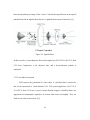
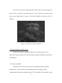
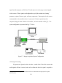
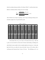
PLANAR LASER-INDUCED FLUORESCENCE (PLIF)
OF
H2 – O2 COMBUSTION
The members of the Committee approve the master’s
thesis of Takashi Yokomae
Frank K. Lu
Supervising Professor
______________________________________
Donald R. Wilson
______________________________________
Seiichi Nomura
______________________________________
Copyright © by Takashi Yokomae 2003
All Rights Reserved
PLANAR LASER-INDUCED FLUORESCENCE (PLIF)
OF
H2 – O2 COMBUSTION
by
TAKASHI YOKOMAE
Presented to the Faculty of the Graduate School of
The University of Texas at Arlington in Partial Fulfillment
of the Requirements
for the Degree of
MASTER OF SCIENCE IN AEROSPACE ENGINEERING
THE UNIVERSITY OF TEXAS AT ARLINGTON
August 2003
ACKNOWLEDGEMENTS
I wish to express my appreciation to my supervising professor, Dr. Frank Lu, for
giving me an opportunity to work on this research at the Aerodynamics Research Center
(ARC), for being patient with my slow progress and for his technical guidance.
I would also like to thank Drs. Wilson and Nomura for being members of my
thesis committee.
Special thanks go to Qiong (Joan) Wei, who has shared her knowledge with me.
I really appreciate those individuals who have assisted me at the ARC: Rod
Duke, Jason Meyers, Chris Roseberry and Philip Panicker, just to name a few.
I am grateful to my mother, Tsugiko, for financial and emotional support from
home back in Japan.
I would also like to acknowledge the teaching assistantship for the first year and
the graduate fellowship for the two years of my graduate study granted by the
Mechanical and Aerospace Engineering Department at the University of Texas at
Arlington.
August 18, 2003
iv
ABSTRACT
PLANAR LASER-INDUCED FLUORESCENCE (PLIF)
OF
H2 – O2 COMBUSTION
Publication No. ______
Takashi Yokomae, M.S.
The University of Texas at Arlington, 2003
Supervising Professor: Frank K. Lu
The fluorescence in the 297-nm wavelength in H2-O2 burning flame is imaged.
A laser sheet is generated when the 248 nm KrF excimer laser beam passes through a
cylindrical lens. Hydroxyl (OH) radical is excited by the laser sheet across the H2-O2
flame produced by a flat flame burner. The excited radical emits fluorescence, which is
captured by the ICCD camera.
However, the fluorescence signal depends on
temperature, as well as OH concentration. In the present work, only fluorescence
images are obtained of the combustion process. Further work is needed to distinguish
between concentration and temperature effects in the fluorescence images.
v
TABLE OF CONTENTS
ACKNOWLEDGEMENTS.......................................................................................
iv
ABSTRACT ..............................................................................................................
v
LIST OF ILLUSTRATIONS.....................................................................................
viii
LIST OF TABLES.....................................................................................................
ix
NOMENCLATURE ..................................................................................................
x
Chapter
1. INTRODUCTION .........................................................................................
1
1.1 Planar Laser-Induced Fluorescence....................................................
1
1.1.1 Laser-Induced Fluorescence.....................................................
1
1.1.2 Planar Laser-Induced Fluorescence..........................................
3
1.1.3 Fluorescence Dependence of
Temperature and Mole Fraction ..............................................
4
1.1.4 Disadvantages of PLIF .............................................................
5
1.2 Objective .............................................................................................
5
2. EXPERIMENTAL SET-UP..........................................................................
7
2.1 KrF Excimer Laser..............................................................................
7
2.2 Combustion System ............................................................................
9
2.2.1 Flat-Flame Burner.....................................................................
9
2.2.2 Combustion Gas Handling System...........................................
10
vi
2.3 Optical System ...................................................................................
13
2.3.1 Spatial Filtering ........................................................................
13
2.3.2 Laser Sheet Generation.............................................................
14
2.3.3 Image Collection.......................................................................
15
2.4 ICCD (Intensified Charged Coupled Device).....................................
15
2.5 Image Acquisition and Processing......................................................
17
2.5.1 Image Collection.......................................................................
17
2.5.2 Image Processing ......................................................................
18
3. RESULTS AND DISCUSSION....................................................................
20
3.1 Results.................................................................................................
20
3.2 Discussion ...........................................................................................
27
4. CONCLUSIONS AND RECOMMENDATIONS........................................
29
4.1 Conclusions.........................................................................................
29
4.2 Recommendations...............................................................................
29
A. EXPERIMENTAL PROCEDURE................................................................
31
B. COMPEX 150 EXCIMER LASER OPERATION PROCEDURE...............
35
C. WINVIEW/32 PROCEDURE ......................................................................
41
REFERENCES ..........................................................................................................
45
BIOGRAPHICAL INFORMATION.........................................................................
47
Appendix
vii
LIST OF ILLUSTRATIONS
Figure
Page
1.1
State View of Laser Induced Fluorescence ..................................................... 2
1.2
Basic Arrangement of PLIF ............................................................................ 4
2.1
PLIF setup ....................................................................................................... 7
2.2
Sectional View of McKenna Flat Flame Burner............................................. 9
2.3
Schematic Diagram of Experimental Setup
for the Flat Flame Burner ................................................................................ 11
2.4
Gas Handling System ...................................................................................... 12
2.5
Spatial Filters................................................................................................... 14
2.6
ICCD Test with 3-D Garfield.......................................................................... 17
2.7
Image Acquisition System Configuration ....................................................... 18
3.1
An Example of WinView/32 Display ............................................................. 23
3.2
Averaging of Five Images ............................................................................... 24
3.3
PLIF Images of Six Cases without Ceramic Rod............................................ 25
3.4
PLIF Images of Six Cases with Ceramic Rod................................................. 26
3.5
Position of Ceramic Rod ................................................................................. 27
viii
LIST OF TABLES
Table
Page
3.1 Results ............................................................................................................. 21
3.2 Correlation Chart for Flowmeters ................................................................... 22
ix
NOMENCLATURE
d
diameter of a lens
f
focal length of a lens
fB(T)
temperature-dependent Boltzmann fraction of the absorbing state
FWHM
full-width at half-maximum
HBW
half bandwidth
ICCD
intensified charge-coupled device
KrF
krypton fluoride
LED
laser emitting diode
& O2
m
mass flow rate of O2
& H2
m
mass flow rate of H2
Spp
fluorescence signal per pixel
T
temperature
UV
ultra violet
VUV
vacuum ultra violet
χOH
OH mole fraction
x
CHAPTER I
INTRODUCTION
As lasers become increasingly available and reliable, laser spectroscopy
becomes promising in the diagnostic probing of combustion processes. Laser-based
techniques are capable of remote, non-intrusive, in-situ, spatially and temporally precise
measurements of chemical parameters, unlike physical probing methods such as
thermocouples that have been traditionally utilized to investigate and characterize
combustion phenomena [1]. Laser-induced fluorescence is presumably the most wellknown technique for radical species measurements. It has been in use considerably
since the early 1980s because of its merits of providing high spatial resolution (typically
0.1 mm), high temporal resolution (typically less than 100 ns), and high sensitivity
(typically concentrations in the ppm range) [2].
1.1 Planar Laser-Induced Fluorescence
1.1.1 Laser-Induced Fluorescence
Laser-induced fluorescence (LIF) is an established, selective and sensitive
approach for identifying species concentration from reactive-flow systems without
perturbing the system under study [3-5]. LIF is a sequence of molecules or atoms being
excited to higher electronic energy states via laser absorption followed by spontaneous
emission of fluorescence.
The spectral absorption regions are discrete, because the
1
energy states of molecules and atoms are quantized. Typically, fluorescence occurs at
wavelengths greater than or equal to the laser wavelength.
Therefore, LIF offers the
possibility to investigate species of interest by selecting the appropriate wavelength.
Shown in Fig. 1.1 below is the state view of LIF. As the species under
investigation are usually molecules or radicals, not atoms, the electronic levels are
divided into sub-levels according to the molecular vibrational and rotational energy.
Due to quantum mechanical effects, electronic, vibrational and rotational energies are
quantized (i.e., 0, 1, 2, …) [6].
Figure 1.1 also shows energy state description of LIF. The molecules or radicals
are excited by laser absorption to the metastable state, and then drop down to the stable
ground state, emitting fluorescence.
Figure 1.1: State View of Laser Induced Fluorescence
2
1.1.2 Planar Laser-Induced Fluorescence
The planar laser-induced fluorescence (PLIF) is a derivative of the LIF
technique, which necessitates the generation of a laser sheet from the probe laser beam
in order to facilitate imaging of the fluorescence. PLIF involves illuminating the flow
with a thin sheet of laser light tuned to excite electronic transitions in a chemical species
in the flow. The OH radical is accessed in this experiment. A radical is an atom or a
group of atoms that is a usually very reactive species, which contains one or more
unpaired electrons. The fluorescence emitted by the laser excitation is focused onto an
intensified charge-coupled device (ICCD) camera to produce an image of the
fluorescence in that region. Besides the species concentration, temperature, pressure
and velocity could be measured with prudent choice of transition and subsequent image
processing [3].
A basic arrangement of PLIF is illustrated below in Fig. 1.2. A laser beam
passes through a cylindrical lens and transforms into a laser sheet. The laser sheet
spreads across the H2-O2 flame produced by a flat flame burner, where it excites the OH
radical, causing it to emit fluorescence. The fluorescence signals are acquired by an
intensified CCD camera. A UV filter and an imaging lens are placed in front of the
ICCD to filter and focus the photo signals.
transmitted to a computer for processing.
3
The images captured by the ICCD are
Figure 1.2: Basic Arrangement of PLIF
1.1.3 Fluorescence Dependence of Temperature and Mole Fraction
The measured quantity of the fluorescence signal, in photons per pixel, from a
single ICCD camera frame can be written as [2]
Spp = const ⋅ χOH ⋅ [fB(T)/T]
The fluorescence signal is directly proportional to the mole fraction of OH and a
temperature-dependent function in brackets. Experimental efficiencies, such as
4
transmission efficiency of the collection lens and filter, the camera’s photo-cathode
quantum efficiency, and the electronic gain on the camera, are considered constant for a
given experimental setup [2].
1.1.4 Disadvantages of PLIF
Just as nothing is perfect, PLIF is not without blemish either.
The main
disadvantage of PLIF is quenching of fluorescence at higher pressures by numerous
collisions of molecules. Such quenching effects can be avoided easily by exciting the
molecule to a fast predissociating state from which fluorescence is emitted only during
the predissociation lifetime. For sufficiently short predissociation lifetimes, collisions
do not occur, which means no quenching within the lifetimes. In some environments
where PLIF is unsuitable, other laser techniques, such as coherent anti-Stokes Raman
scattering (CARS) or Rayleigh scattering are recommended [7].
1.2 Objective
In long duration facilities, flow parameters could be measured with physical
probes that are placed spatially through the flow. However, this method is not suitable
for pulsed flow facilities, because of their short flow duration. A desirable alternative to
such probe-based methods in pulsed facilities is PLIF imaging, which yields
instantaneous measurements at a large number of points in a laser-illuminated plane [8].
The development of pulse detonation engines is underway at the Aerodynamics
Research Center. The initiation of detonation is believed to occur at “hot spots” [9]
5
where heat and pressure are sufficient to trigger a rapid chemical reaction. In oxyhydrogen systems that involve chemical activity, a large population of OH is expected.
This OH formation can be studied by the use of PLIF, since OH is one of the species
that can be detected in PLIF measurements.
The objective of this research is to visualize OH formation within oxy-hydrogen
combustion by means of PLIF, as a stepping-stone to the next phase of experiments in
detonation waves.
6
CHAPTER II
EXPERIMENTAL SET-UP
The PLIF set-up without combustion system is shown in Fig. 2.1 below. The
combustion system is depicted in section 2.2.
Ceramic rod
Cylindrical lens
Beam shutter
Excimer
laser
Beam
stop
WinView
display
Flat
flame
burner
ICCD
Coolant circulator
ICCD detector controller
Figure 2.1: PLIF set-up
2.1 KrF Excimer Laser
Excimer stands for excited dimer, a diatomic molecule usually of a rare gas
atom and a halide atom that are bound in excited states only. ArF, KrF, XeCl and XeF
7
are the most important excimers, because they dissociate releasing the excitation energy
through UV photons [10].
The energy is high-intensity beams of UV light with
wavelengths ranging from 193 to 351 nm [11]. When compared with visible light
sources, UV lasers are capable of detecting minor species, such as, OH, NO, and CO
[12]. The OH radical is naturally occurring [2] and one of the most abundant in flames
[6].
In this experiment, a COMPex 150T KrF Excimer Laser (Lambda Physik) was
used, because its center wavelength and bandwidth are tunable between 248.0 and 248.8
nm and it coincides with some of the OH A-X (3,0) band system [12]. The absorption
line of OH is excited at 248 nm [A2Σ+(ν’=3)ÅX2Π (ν”=0)] and detected at 297 nm
[A2Σ+(ν’=3)ÆX2Π (ν”=0)]. Despite the weaker strength of this OH transition than
others that could be used, such as 284 and 308 nm, there are advantages of using 248
nm. Excitation of the OH radical at 248 nm not only minimizes the dependence of the
resulting fluorescence on quenching effects, but also maximizes the predissociationdominated decay process. “Predissociation occurs when the potential energy curve for a
bound molecular state is crossed by the curve of a repulsive, or unbound, state” [2].
Selecting this particular LIF approach enables the specifically-sensitive measurement of
OH concentration in the flow.
This approach has previously been used in OH
measurement of an automobile engine, in a laboratory-scale, supersonic, H2-air
combustion tunnel, etc. [2].
The laser pulse energy is maximum at 380 mJ/pulse at low repetition rates (< 10
Hz, or pulses/sec.). However, the laser was operated at 20 Hz with a constant pulse
8
energy of 50 mJ/pulse set by a designated computer for the laser. Pulse length is
typically 22 nm, which is fast enough to freeze flows [2].
2.2 Combustion System
2.2.1 Flat-Flame Burner
A “laboratory-standard” [2], McKenna flat flame burner is used, as shown
below in Fig. 2.2.
(4.72 in)
(2.36 in)
Figure 2.2: Sectional View of McKenna Flat Flame Burner
The burner is made up of a 6-cm-diameter sintered porous stainless-steel plug
and a 1.4-cm-width sintered porous bronze shroud ring. The reactant mixture consisting
9
of pre-mixed oxidizer (O2) and fuel (H2) is introduced into the bottom of the burner and
distributed over the cross section by the sintered plug. Any existing surge in the reactant
stream is settled in the cavity located below the sintered plug. Passing a concentric inert
gas (N2) around the flame holder through the bronze plug ring enables shielding of the
flames produced from entrainment effects and stabilizes the flame above the sintered
plug. This shielding gas is also brought into a cavity in the bottom of the burner in order
for any surge present to be damped out. The cooling water is supplied to the burner by a
stainless-steel tubing, where it is rolled in a spiral shape with equally spaced rings and
embedded in the sintered plug. The plane of the coil is parallel to the surface of the
burner to ensure that radial temperature gradients do not occur [13].
2.2.2 Combustion Gas Handling System
List of Equipment
a. Compressed hydrogen (~200 ft3 cylinder, Airgas)
b. Compressed oxygen (~80 ft3 cylinder, Airgas)
c. Compressed nitrogen (~200 ft3 cylinder, Airgas)
d. Pressure Regulators
e. Flashback arrestors (Ibeda Inc.)
f. Correlated flowmeter with standard valve (Cole-Parmer)
g. Copper, steel and plastic tubing
h. Standard temperature millboard (McMaster-Carr)
10
Figure 2.3 illustrates the setup for the combustion system, and Fig.2.4 is the
picture of the gas handling system.
Figure 2.3: Schematic Diagram of Experimental Setup for the Flat Flame Burner
11
Regulator for O2
Regulator for H2
Flowmeter
for H2
Flowmeter
for O2
Flowmeter for N2
H2
O2
Flash arrestor for H2
Flash arrestor for O2
Figure 2.4: Gas Handling System
Oxygen and hydrogen gas cylinders with pressure regulators are fixed on the
side of the combustion table. The millboard (40 inch wide by 42 inch high) is erected
between the burner and the gas cylinders for safety. The gases from two cylinders are
joined at a tube union, and hence pre-mixed before ignited at the burner. To prevent
backflash upon ignition, two flash arrestors are installed: one between the O2 cylinder
and the union, the other between the H2 and the union. In addition, to adjust the flow
rates of gases, correlated flowmeters with standard valves (Cole-Parmer catalog nos. A-
12
03216-22 for O2 and H2, and A-03216-32 for N2) are installed. A vertical tangential
locator line of a flowmeter ensures accuracy in reading the float position.
2.3 Optical System
The optical system consists of spatial filtering, laser sheet generation and image
collection.
List of Equipment
a. Spherical plano-convex objective lens: f ~ 350 mm, d = 2 in (CVI Laser)
b. Pinhole: 40 µm diameter
c. Cylindrical plano-concave lens: f ~ -81.4 mm, d = 1 in (CVI Laser)
d. Spherical plano-convex imaging lens: f ~ 50 mm, d = 1 in (CVI Laser)
e. Band-pass filter: center wave length 296.7 ± 10 nm (HBW or FWHM),
d = 1 in (CVI Laser)
f. Optical table rails & carriers (Thermo Oriel)
2.3.1 Spatial Filtering
Spatial filters eliminate random fluctuations from the intensity profile of a laser
beam, which increases resolution significantly. Optical defects and particles in the air
cause intensity variations of laser beams. Spatial filtering is fairly simple (see the
schematic shown in Fig. 2.5). An ideal coherent, collimated laser beam behaves as
though produced by a distant point source. Spatial filtering consists of focusing the
13
beam and producing an image of the “source” with all the imperfections in the optical
path defocused in an annulus about the axis. A pinhole blocks most of the noise [14].
Figure 2.5: Spatial Filters
In this research, a 2-inch-diameter fused silica singlet lens, PLCX-50.8-180.3-UV from
CVI Laser Corporation, is the objective lens, and a 40-µm-diameter pinhole is
employed.
2.3.2 Laser Sheet Generation
PLIF requires the generation of a laser sheet. A cylindrical lens is used to do
this. In the experiment, a 1-inch-diameter VUV CaF2 round singlet lens, CLCC-25.438.1-CFUV from CVI Laser, is used. Calcium fluoride negative cylindrical lenses are
appropriate for anamorphic expansion at vacuum ultra-violet wavelengths. They are
ideal for use with excimer lasers [15].
14
The excimer laser first passes through the objective lens, cleaning the scattering
from dust particles [14]. It then goes through the pinhole, creating a “clean” [14] spatial
profile. Subsequently, it passes through the cylindrical lens, producing the laser sheet.
2.3.3 Image Collection
A narrow band interference filter with center wavelength of 296.7 ± 10 nm
(F10-296.7-3-1.00 from CVI Laser) is selected (see Section 2.1).
An ICCD camera
with the filter mounted onto, is placed at right angles to the laser sheet. This will let
only the selected fluorescence pass and block undesirable ambient light, scattered laser
light at 248nm and emission from the flame [2].
A 1-inch-diameter fluorescence-imaging lens (fused silica single lens, PLCX25.4-25.8-UV from CVI Laser) is placed about 50 mm away from the ICCD intensifier,
with the convex side facing the ICCD, and focuses the image into the ICCD. The
optical table rail and carrier were used to fix the lens onto the table.
2.4 ICCD (Intensified Charged Coupled Device)
List of Equipment
a. ICCD detector (Princeton Instruments)
b. ICCD detector controller (Princeton Instruments)
c. Coolant circulator (Princeton Instruments)
d. Ultra high purity, compressed nitrogen (Airgas)
15
The ICCD detector (Model ICCD 576 E) from Princeton Instruments (PI) has a
384 x 576 pixel format. The front enclosure of the ICCD detector includes the image
intensifier and the CCD. The image intensifier is coupled to the CCD using a fiber
optic window on both the output of the image intensifier and the front side of the CCD.
Due to the1:1 coupling ratio, the fiber optics translates the output of the image
intensifier to the input of the CCD at the same size. This type of coupling is the most
efficient possible, as well as eliminating lens effects such as vignetting.
“The CCD array in an ICCD camera is cooled by a Peltier-effect
thermoelectric cooler, driven by closed-loop proportional-control circuitry. A thermal
sensor attached to the cooling block of the detector monitors its temperature. The
coolant block is made of Delrin to prevent condensation, but this also prevents heat
transfer from the thermoelectric cooler to the atmosphere. Water or other coolant is
therefore necessary to carry away heat generated by the thermoelectric cooler [16].”
The ICCD is typically operated cooled (≥ -45°C) with chilled water circulation, with the
help of a coolant circulator, Model CC-100, also provided by PI.
The ICCD needs continuous flushing of the detector with nitrogen while
operating cooled. Even if the detector is not powered, flushing is required whenever the
coolant is circulating, in order to prevent moisture condensation. Since PI recommends
nitrogen with less than or equal to 10 ppm, compressed nitrogen of grade ‘ultra high
purity’ from Airgas is used.
The ICCD is controlled by the detector controller, Model ST 138-S, from PI
which sends information to a computer through a TAXI cable and PCI interface card.
16
The ICCD was tested in visible light with a Nikon lens with a focal length of 1
meter (3.28 ft), with all the room lights shut off. The UV filter was removed and the
laser was not firing. Figure 2.6 shows a 3-D object (Garfield, also shown in Fig. 2.1)
acquired.
Figure 2.6: ICCD Test with 3-D Garfield
2.5 Image Acquisition and Processing
The ICCD controller is managed by WinView/32 software from PI. The
fluorescence images acquired are stored on the host computer (Windows98), processed
and displayed.
2.5.1 Image Acquisition
The WinView/32 software, also from PI, is installed on the host computer
(Windows98). The PCI interface card installed in the host computer permits
communication between the computer and the ST-138 controller. The controller accepts
17
input from the computer, or WinView/32, and converts it to the proper control signals
for the camera. These signals can be adjusted to specify the readout rate, binning*
parameter, regions of interest, gain, and array temperature. Data acquired in the camera
is transmitted to the controller where it is processed. It then is passed on to the
computer, displayed in the WinView/32 window, and can be stored on disk [17]. The
system configuration is presented in Fig. 2.7 below.
Figure 2.7: Image Acquisition System Configuration
2.5.2 Image Processing
PI systems are adjusted so that data have a small offset. This offset assures that
small signals will not be missed, and can be subtracted after the signal is acquired to
*
The specified number of pixels in each direction will be combined to form super pixels for greater
sensitivity [17].
18
prevent it from having any influence on the data. The background subtraction feature
automatically subtracts any constant background in the signal. This includes not only
constant offsets caused by the amplifier system in the controller, but also timedependent buildup of dark charge. The background subtract equation is expressed as
follows [17]:
Corrected image data = Raw image data – Background
Another data correction technique, flatfield correction, which divides out nonuniformities in gain from pixel to pixel, was also available in WinView/32, but was not
used, because this was found to be unnecessary.
The corrected images are displayed in WinView/32. Gray-scale images can be
displayed in false color, which varies with the light intensity or the fluorescence signal.
Five frames of images are averaged, since the flame fluctuate even with nitrogen
shielding, mostly because of air-conditioning.
19
CHAPTER III
RESULTS AND DISCUSSIONS
This chapter presents the PLIF results obtained and the interpretation of the
results. The experimental procedures are detailed in Appendices A - C.
3.1 Results
The laser repetition rate (20 Hz), laser energy (50 mJ/pulse), camera position
and focus and camera filters are kept constant during the experiments. The PLIF
technique was employed to capture images of fluorescence emitted by the 248 nm KrF
excimer laser excitation, while varying mixture ratio, or controlling the volumetric flow
rates of hydrogen and oxygen. Mixture ratio (MR) is defined as the ratio of the oxidizer
to fuel mass flow rates [2]. A ceramic rod was also inserted in the flames,
perpendicular to the laser sheet, to stabilize the flame [18].
In the case of the fuel being H2 and the oxidizer O2, the reaction is expressed as:
2 H2 + O2 Æ 2 H2O
So, the stoichiometric MR for H2-O2 combustion is calculated as 8.
& O2
m
& H2
m
=
1 mol * 32 g / mol
=8
2 mol * 2 g / mol
A number of PLIF images were taken at various mixture ratios, listed in Table
3.1. The values for volumetric flowrates [ml/min] in Table 3.1 are taken or interpolated
20
from the correlation charts provided by Cole-Parmer (Table 3.2), and the mixture ratios
(MR) are calculated as follows, taking case one for example.
& O2
m
& H2
m
459 ml / min
* 32 g / mol
22400 ml / mol
=
= 3.627 ,
2025 ml / min
* 2 g / mol
22400 ml / mol
where 22400 ml is the volume occupied by 1 mole of a gas, assuming an ideal gas, and
molecular weight of O2 is 32 g/mol and H2 2 g/mol.
Table3.1: Results
Case H2 [mm] H2 [ml/min] O2 [mm] O2 [ml/min] N2 [mm] N2 [ml/min] Ceramic
1
20
2025
15
459
60
12724
No
2
20
2025
15
459
60
12724
Yes
3
25
3000
15
459
60
12724
No
4
25
3000
15
459
60
12724
Yes
5
30
4162
15
459
60
12724
No
6
30
4162
15
459
60
12724
Yes
7
18
1639
15
459
40
9608
No
8
18
1639
15
459
40
9608
Yes
9
20
2025
17
575
40
9608
No
10
20
2025
17
575
40
9608
Yes
11
20
2025
20
749
40
9608
No
12
20
2025
20
749
40
9608
Yes
MR
3.627
3.627
2.448
2.448
1.765
1.765
4.481
4.481
4.543
4.543
5.918
5.918
The maximum flow of O2 was 20 mm or 749 ml/min for this setup. When the
O2 flow rate was increased over that value, the burner started making a whistling noise
and the flame became unstable, which eventually might have been put out. On the other
hand, the H2 flow rate could not be lowered less than 18 mm or 1639 ml/min, while it
could go up to the flowmeter limit, 65 mm or 13.6 l/min.
21
The shielding gas, N2, was
kept constant at 60 mm or 13.4 l/min for the first six cases, where the flame was
relatively larger, and lowered to 40 mm or 96.1 l/min for relatively small flame.
Table3.2: Correlation Chart for Flowmeters
Scale Reading
H2 [ml/min] O2 [ml/min] N2 [ml/min]
[mm]
65
13600
3761
13412
60
11875
3395
12724
55
10360
3051
12049
50
9302
2727
11252
45
7600
2400
10450
40
6450
2098
9608
35
5176
1787
8753
30
4162
1451
7777
25
3000
1108
6748
20
2025
749
5626
15
1060
459
4502
10
430
251
3313
5
178
120
2056
An example of WinView/32 display is shown in Fig. 3.1 below. The image is
rotated 90 degrees counter-clockwise. Colors are assigned according to intensity of
fluorescence captured by the ICCD, low intensity being black and high being red. The
range of the intensity level was kept at 300 to 1200, after examining all the images.
Vertical and horizontal cross-sections profile the intensity at the strips where the cursor
(shown as a big white cross) is placed. High intensities shown at the bottom of the
image can be assumed to be the fluorescence emitted at the beam stop (see Fig. 2.1) that
reflected back and is removed during further processing.
22
Burner
Fig. 3.1 An Example of WinView/32 Display
Figure 3.2 demonstrates averaging of five images for Case 1. The reason why
the averaging was done is because the flame flickers somewhat. Figures 3.3 and 3.4
show the averaged images for the twelve cases. At each MR, a ceramic rod was inserted
to stabilize the flame [18] (Fig. 3.4). The position of the rod is 0.44 in. above the burner
surface and 0.31 in. to the right from the vertical centerline of the burner, as described
in Fig. 3.5. The burner is outlined with white lines in each image. For Cases 7 and
later, the ICCD was accidentally moved and the image frame also moved slightly.
23
5.4 in
4.1 in
(a) Test 1
(b) Test 2
(c) Test 3
(d) Test 4
(e) Test 5
(f) Average
Figure 3.2: Averaging of Five Images
24
5.4 in
4.1 in
(a) Case 1: MR = 3.627
(b) Case 3: MR = 2.448
(c) Case 5: MR = 1.765
(d) Case 7: MR = 4.481
(e) Case 9: MR = 4.543
(f) Case 11: MR = 5.918
Figure 3.3: PLIF Images of Six Cases without Ceramic Rod
25
5.4 in
4.1 in
(a) Case 2: MR = 3.627
(b) Case 4: MR = 2.448
(c) Case 6: MR = 1.765
(d) Case 8: MR = 4.481
(e) Case 10: MR = 4.543
(f) Case 12: MR = 5.918
Figure 3.4: PLIF Images of Six Cases with Ceramic Rod
26
0.31 in.
0.44 in
Figure 3.5: Position of Ceramic Rod
3.2 Discussion
The flame was asymmetric for the cases without the ceramic rod, but this was
because the flame was non-uniform: the flame was always generated on the right side of
the burner, seen from the ICCD. However, after inserting the ceramic rod, the flame
became more uniform. The flame in Fig. 3.4 is more uniform than that in Fig. 3.3.
The stoichiometric mixture ratio of 8 was not achieved, due to restriction of the
gas handling system, or the burner.
In both Figs. 3.3 and 3.4, it can be seen that lower the mixture ratio (MR), the
larger is the flame image. As mentioned in section 1.1.3, the measured quantity of the
27
fluorescence signal is written as, Spp = const ⋅ χOH ⋅ [fB(T)/T]. The fluorescence signal is
directly proportional to the mole fraction of OH and a temperature-dependent function
in bracket.
As the MR increases, both adiabatic flame temperature (T) and OH mole
fraction (χOH) increase¥. In this situation, it is difficult to separate the χOH term from the
[fB(T)/T] term, since when χOH increases, 1/T decreases while fB(T) varies with
temperature, too.
In the experiments, it appears that the temperature effect was dominant. In other
words, as MR increased, χOH increased, but the [fB(T)/T] term decreased much more,
causing the fluorescent to decrease. It is problematic to say that the OH concentration is
directly proportional to the fluorescence signal.
The spatial filters discussed in Section 2.3.1 were not used, because the strong
laser burned the pinhole. After removing the pinhole and the objective lens, decent
laser sheet was still generated and the experiment was continued.
¥
From personal communication with Dr. D. R. Wilson, who used hypersonic air-breathing propulsion
code.
28
CHAPTER IV
CONCLUSIONS AND RECOMMENDATIONS
4.1 Conclusions
The objective of the study was to visualize the hydroxyl (OH) formation within
the hydrogen-oxygen combustion by means of PLIF, which is suitable for use in pulsed
facilities. The conclusions drawn from the investigation are summarized as follows:
1. Stoichiometric mixture ratio of 8 was not attained.
2. As the MR increased, the fluorescence signal decreased.
3. The planar laser-induced fluorescence of the OH radical was acquired
successfully, however, if it can be directly reflected in OH concentration is in
question.
4.2 Recommendations for Future Work
The burner needs repairing in order to get a uniform flat flame, as well as to
reach stoichiometric mixture ratio.
In addition, a UG-11 Schott glass filter may be useful to block the 445-nm
second transmission band of the 297-nm bandpass filter, as employed in experiments in
[2], where they have the same experimental setup: the same KrF excimer laser and the
same 297-nm filter.
29
Although the images were taken by single shot Free Run mode, the whole image
acquisition setup can be integrated by introducing a PG-200 pulse generator. The pulser
can synchronize the laser, ICCD detector and ST-138 detector controller, when used as
a master trigger. This will eliminate the possibility of missing the fluorescence signal by
the ICCD.
Further study should be performed for the future applications of PLIF. With
more sophisticated equipment, temperature and velocity measurements can be achieved.
30
APPENDIX A
EXPERIMENTAL PROCEDURE
31
1. Ensure the following connections:
a. Connect a 25-pin ICCD cable from the ICCD to “Detector” of the ST-138
controller.
b. Connect a TAXI cable from “J7” of the ST-138 controller to the PCI
interface card of the computer with WinView/32 software installed.
c. Ensure the coolant hoses and N2 hose are connected to the ICCD.
2. Place the cylindrical lens about 23.5 inches from the burner, with the concave side
facing the laser.
3. Place the ICCD camera as close to the burner as possible (about 20 inches) at the
right angle to the laser sheet. Also place the imaging lens about 50 mm from the
image intensifier of the ICCD, with the convex side facing the ICCD. Since the
bandpass filter is mounted on the ICCD, the imaging lens is almost touching the
ICCD.
4. Power the laser assembly, designated computer and monitor for the laser. Open the
water valve. See Appendix B for the details of the laser operation.
5. Ensure all the valves of the four flowmeters are closed.
6. Open the nitrogen cylinder valve. Adjust the pressure regulator to about 15 psi (1
bar). Then open the gas line.
7. Power the ST-138 detector controller, switch on the cooling of the ST-138, and
power coolant circulator CC-100. The ST-138 will be ready (temperature is
thermostated to within ±0.050 °C of preset value; in this case, -30 °C) in about 10
minutes when the status LED is turned from orange to green.
32
8. Immediately after procedure 8, open the valve of the flowmeter of the nitrogen for
the ICCD and set it to 1~2 liters/min for at least 10 minutes, and then lower to
0.75~1 liters/min. The flowmeter is for air (molecular weight of about 28.8 g/mol),
but it can be used in the same way since it is close to that of nitrogen (28 g/mol)
and accurate flow rate is not required. One division equals 1 liters/min.
9. Power host computer for WinView/32 and monitor. Start the WinView/32
software. If you start WinView/32 before you turn on ST-138, you will see
“Controller is not responding!” See Appendix C for WinView/32 operation
procedure.
10. Open the valves of O2 and H2 cylinders. Set the pressure regulators to about 15 psi
(100 kPa). Open the gas lines.
11. Open the flowmeter valve for H2 and ignite the burner with a long match. The
flowmeter reading should be about 20 mm. Turn off the room lights in order to see
the flame better. Open the flowmeter valve for O2, too, and adjust it to about 15
mm. Always ignite fuel (H2) first!
12. Open the flowmeter valve for N2 and adjust it to the maximum value, 60 mm, or
until you do not see orange flame any more. Orange flame means it is reacting with
ambient air and the N2 shielding is not sufficient.
13. Fire the laser. See Appendix B for the laser operation procedure.
14. “Acquire” the image with WinView/32. See Appendix C for the WinView/32
procedure.
33
15. Change mixture ratio of the H2 and O2 and acquire more images and repeat. Also,
insert ceramic rod to stabilize the flame [18].
16. After the experiments, turn off everything. Do not forget to close the water valve,
as well.
17. After turning off the ST-138 controller, keep flushing the ICCD with nitrogen at a
flowrate of at least 2 liters/min for at least 30 minutes. This keeps moisture
condensation from forming on the ICCD until it reaches room temperature.
34
APPENDIX B
COMPEX 150 EXCIMER LASER OPERATION PROCEDURE
35
I. Starting the Laser Assembly
Keep in mind that the laser assembly consists of Amplifier and Oscillator.
1. Check the beam path.
2. Turn on main switch of the laser assembly at the utility supply.
3. Turn on main switches and key switches of both Amplifier and Oscillator.
4. Switch on the designated computer (PC) and the monitor. Always turn on the laser
assembly before turning on the computer to prevent data ring diagnosis failure (see
section II. 1. below).
5. Wait until DOS-prompt C:\> and a blinking cursor appears.
6. Type “cd lambda” to change directory.
7. Type “lc150” to start the COMPex150 software.
II. Booting the Local Software
After the software started, it passes three tests:
1. Data ring diagnosis (also called dynamic fiber loop check)
The data ring of the COMPex 150 is a local area network (LAN), which links
the modules of the laser assembly with fiber optics lightwave guides. To test it, the
PC sends a light signal and checks if it passes the LAN. If this test fails, a window
“DYNAMIC FIBER LOOP CHECK” appears.
When this happens, turn off both the PC and the laser assembly and wait for
about 30 minutes and turn them back on.
If everything is all right, the program enters the module availability check.
36
2. Module Availability Check
This tests what modules of the laser assembly are recognized by the PC. If any
of them does not respond, NOT INSTALLED is displayed and a beep tone is
displayed. However, because the last one, F2-SOURCE, is not installed, just hit G to
continue if everything else is YES. The F2-source is an extra part that could generate
the fluorine (F2) gas when the laser is turned on, but in our configuration, the F2 gas
in the gas cabinet is used.
Upon pressing G, the program continues with the self test.
3. Self Test
The self test shows the results of the data ring diagnosis and checks the
COMPex watchdogs. Afterwards, it sets the stepper motor of the grating to its last
position.
Motor reference position once failed. The grating is controlled via a small
stepper motor. When the laser is powered on this motor will drive in one direction
until it sees an optical "flag" and then stop. This is the motor’s way of finding
"home". If it doesn't find "home" then the software will give this error. This problem
was solved by turning the drive motor pulley with fingers in such a direction to drive
the grating in the opposite direction about half an inch with the main power off.
Then turn on the main power and watch the motor move the grating.
If the test results are OK, the program begins to wam-up the thyratron and
enters the Main Menu. It takes about 8 minutes to warm up.
37
III. Main Menu – The Central Program Menu
1. Check current settings on Main Menu.
2. Press M to open the Data Menu.
Notice that both laser devices (Ampl. for Amplifier and Osc. for Oscillator) are
represented with their own page. The Oscillator page is the master page;
parameters in Amplifier are ignored.
Check Parameter Setting of the Oscillator as follows:
a. Excimer gas and its wavelength (KrF, 248 nm)
b. Buffer gas (Ne for KrF)
c. Repetition rate (20 Hz)
d. Trigger mode (internal)
e. Running mode and its preset parameter (Energy Constant mode at 50mJ)
It is possible to change the gas values, but it is not recommended since
the preset gas values are carefully optimized.
3. Laser Firing
a. Open the water valve over the stairs.
The laser has to be cooled with water at repetition rates higher than 10 Hz.
b. Open the beam shutter.
c. Type S, and then Y to confirm.
The laser now needs a few seconds to initialize the power supply. The menu
changes to the Running Menu. Then is begins emitting laser light with the given
38
repetition rate. It can be recognized by clicking noise. The higher the repetition rate
is, the faster the clicking will be.
All the gas valves remain closed while firing the laser.
d. If the laser beam seems weak, New Gas Fill has to be performed.
IV. Conditions Before Starting New Fills
1. The laser must not be firing.
2. Make sure that all the four required gases are available.
Do not use gas cylinders with less than 74 psi (5 bar), since the impurities from
gas cylinder walls can contaminate the tube.
3. Turn on the vacuum pump of the gas cabinet.
4. Open all the four gas cylinder valves in the gas cabinet.
5. Close all the four pressure regulators in the gas cabinet.
6. Ensure all the four pressure regulators are set to about 60 psi (4 bar).
7. Open all the gas lines, marked with post-it notes.
V. New Gas Fill (automatic)
1. Go to the Main Menu and press M to enter the Data Menu.
2. Press N and select the page with KrF Osc. or KrF Ampl. that needs a new fill.
39
---------------------------------------VERY IMPORTANT---------------------------------------The New Fill procedure fills the laser device that is actually the upper most page on the
Data Menu. You have to fill Oscillator and Amplifier, separately. To change the page
on the Data Menu, hit N for next page.
---------------------------------------VERY IMPORTANT----------------------------------------
3. Push Q to leave the Data Menu. Now you are on the Main Menu.
4. Push G to open the Gashandling Menu.
5. Push N to start a new fill.
The laser tube is evacuated to 30 mbar. If the evacuation exceeds 12 minutes,
there may be a gas leak. The gases will be filled one by one for the amount specified.
The new fill will stop automatically when it is filled to 3330 mbar.
40
APPENDIX C
WINVIEW/32 OPERATION PROCEDURE
41
1. Start WinView/32. Unless the ST-138 is powered, “Controller Is Not Responding!”
will appear.
If the ST-138 is on and the message still shows up, the pins of the
TAXI cable is most likely torn. Check the pins of the cable with continuity test of a
multimeter. The TAXI cable has only four wires in it:
pin # 2 connects to pin #4 on the opposite side
pin # 7 connects to pin #9 on the opposite side
pin # 4 connects to pin #2 on the opposite side
pin # 9 connects to pin #7 on the opposite side
Once you find discontinuities, dismantle the both ends of the cable and solder the
pins.
2. In Setup | Hardware | Interface tab, select “High Speed PCI”.
In Setup | Hardware Controller/Camera tab, select “ST 138” for Controller Type,
“EEV 576x 384 [3ph]” for Camera Type, “Electronic” for Shutter Type and check
“Full Frame” for Readout Mode.
3. Go to Acquisition | Experimental Setup.
a. In Main tab, select “0.1 sec” for Exposure Time, “1” for Number of Images, and
“1” for Accumulations. Also check “Use Full Chip” for CCD Readout.
b. In Timing tab, select “Free Run” for Timinig Mode and “Normal” for Shutter
Control.
c.
In Data File tab, type in Data File Name a file name you want to create, such as
073103Test. Click on “Enable” for Auto Increment File Name and set Current
42
Value to “1”. This will facilitate the file handling by adding the suffix with
incrementing numbers from 1, as 073103Test1, 073103Test2 and so on.
d. In ROI tab, select “1” for New Pattern, “1”, “380” and “5” for X, and “1”,
“575”, “5” for Y.
4. The proper position of the ICCD can be checked with Flat Field images, although
flat field is not used for the right purpose. With the room lights on, take flat field by
“Acquisition | Acquire Flat Field.” You will see high intensities caused by
fluorescent lights on the sides of the burner on the image. Using these clues, move
the ICCD to the right position.
5. Acquire background for background correction, by selecting Acquisition | Acquire
Background. Then in Acquisition | Experimental Setup | Data Correction tab, select
the background file. Make sure the Flat Field box is unchecked. Flat Field feature
is not used, because it does not improve the images in this particular experiment.
6. Turn off the room lights, ignite the burner, adjust the flowrates to desired mixture
ratio and fire the laser. Acquire images by selecting Acquisition | Acquire. A blackand-white picture will be shown on display.
7. Change flowrates of the H2 and O2 gases and repeat 5. Also, insert a ceramic rod to
stabilize the flame [18] and repeat 5.
8. Gray-scale images can be converted to color images by color icon.
9. In Display | Display Layout | General tab, Axes, Cross Sections and Info Bar boxes
are checked to make analysis easier.
10. In Display | Display Layout | Range tab, Intensity level can be manually selected.
43
11. Since WinView/32 can be run only on Windows 98 machine (we have license only
on Windows 98), press “Print Screen” on the keyboard, paste onto wordpad and
save as Word 6 file in order to make color copy. This can be seen and edited in
Microsoft Photo Editor on other machines
44
REFERENCES
1. Eckbreth, A. C, “Laser Diagnostics for Combustion Temperature and Species”,
Abacus Press, Kent UK and Massachusetts USA, 1988.
2. Cohen, L.M., Jassowski, D.M., and Ito, J.I., “Performance of a Titan rocket engine
using laser-induced fluorescence of OH”, AIAA Journal, Vol. 39, No. 10, pp. 19261935, October 2001.
3. Houwing, A.F.P, Smith, D.R., Fox, J.S., Danehy, P.M., & Mudford, N.R., “Laminar
boundary layer separation at a fin-body junction in a hypersonic flow”, Shock
Waves, Vol. 11, pp. 31 - 42, 2001.
4. Bessler, W.G., Hildenbrand, F., & Schulz, C., “Two-line laser-induced fluorescence
imaging of vibrational temperatures in a NO-seeded flame”, Applied Optics, Vol.
40, No. 6, pp. 748 - 755, 2001.
5. Rothe, E.W., and Andresen, P., “Application of tunable excimer lasers to
combustion diagnostics: a review”, Applied Optics, Vol. 36, No.18, pp. 3971 –
4033, 1997.
6. Bombach, R., “Laser Spectroscopy in Combustion Research”, Ch.2, Paul Scherrer
Institut, Switzerland, Internet URL: http://cdg.web.psi.ch/Summerschool/chap2.pdf.
7. Anderson, P., Bath, A., Gröger, W., et al, “Laser-induced fluorescence with tunable
excimer lasers as a possible method for instantaneous temperature field
measurements at high pressures: checks with an atmospheric flame”, Applied
Optics, Vol. 27, No. 2, pp. 365 – 378, 1988.
8. Houwing, A.F.P., Palma, P.C., et al, “Fluorescence-imaging-based flow diagnostics:
applications to free-piston shock tunnel flows”, 22nd International Symposium of
Shock Waves, Imperial College, London, UK, July 18 – 23, Paper 0890, 1999.
45
9. Oran, E.S., and Khokhlov, A.M., “Deflagrations, Hot Spots, and the Transition to
Detonation”, 17th International Colloquium on the Dynamics of Explosions and
Reactive Systems, Heidelberg, Germany, July 25 - 30, 1999, Internet URL:
http://www.iwr.uni-heidelberg.de/~icders99/program/papers/001-050/031.pdf.
10. Databank Oxydex, Internet URL
http://www.databank.oxydex.com/science_mathematics_references/excimer_lasers.
html.
11. Lambda Physik Inc., “User Manual COMPex 150”, Ft. Lauderdale, Nov., 1997.
12. Chen, Y.-C., Mansour, M.S., “Topology of turbulent premixed flame fronts
resolved by simultaneous planar imaging of LIPF of OH radical and rayleigh
scattering”, Experiments in Fluids, Vol. 26, pp. 277 - 287, 1999.
13. Prucker, S., Meier, W., & Stricker, W., “A flat flame burner as calibration source
for combustion research: Temperatures and species concentrations of premixed
H2/air flames”, Review of Scientific Instruments, Vol. 65, No. 9, pp. 2908 – 2911,
Sept., 1994.
14. Newport Corporation, “Spatial Filter”, Internet URL:
http://www.newport.com/file_store/PDFs/tempPDFs/Spatial_Filters_e3873.pdf.
15. Lambda Research Optics, Inc., Internet URL: http://www.lambda.cc/PAGE51.htm.
16. Roper Scientific, “ICCD Detector Operation Manual”, 1999, Internet URL:
ftp://ftp.roperscientific.com/manuals/files%5C0009v3f.pdf.
17. Roper Scientific, “WinView Princeton Instruments Imaging Software”, 2001,
Internet URL: ftp://ftp.roperscientific.com/manuals/files%5C0046v25b.pdf.
18. Hanson, R.K., Seitzman, J.M., & Paul, P.H., “Planar Laser-Fluorescence Imaging of
Combustion Gases”, Applied Physics B, Vol. 50, pp. 441 - 454, 1990.
46
BIOGRAPHICAL INFORMATION
Takashi Yokomae received his Master of Science in Aerospace Engineering
from the University of Texas at Arlington (UTA) in December 2003. He was born in
Japan and upon completing high school there, he came to the United States to study in
the University. He received his Bachelor of Science in Aerospace Engineering from
UTA in May 2003. Culturally diverse UTA community allowed him to be more broadminded during his 6-year stay at UTA. He likes to play various kinds of sports: for
example, basketball, tennis, baseball, softball, swimming and rollerblading.
47