Download CASCA: A Simple 2-D Mesh Generator

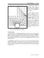
CASCA: A Simple 2-D Mesh Generator
Version 1.4 User's Guide
May, 1997
Manual and Code Modifications by:
Daniel Swenson, Mark James, and Brian Hardeman
Kansas State University • Manhattan, Kansas
CASCA originally written by:
Paul Wawrzynek and Louis Martha
Cornell University • Ithaca, New York
Page ii
Table of Contents
Table of Contents
Introduction.....................................................................................................................1
CASCA Files ...................................................................................................................3
CASCA *.csc Files....................................................................................................3
VIEW *.vw Files .......................................................................................................3
Input *.inp Files.........................................................................................................3
CASCA Examples...........................................................................................................5
Plate with Hole Using Symmetry .............................................................................6
Running the CASCA Program...............................................................................6
Set Scale: Setting an Appropriate Data Space......................................................6
Geometry: Creating the Problem Outline ..............................................................7
Subregions: Dividing the Geometry......................................................................8
Subdivide: Specifying Nodal Points on the Edges................................................8
Mesh: Mesh Generation for Plate .........................................................................9
Example with Complete Hole and Different Meshing Algorithms ........................11
Run CASCA .........................................................................................................11
Set Scale...............................................................................................................11
Geometry..............................................................................................................11
SubRegions:..........................................................................................................11
Subdivide the Edges .............................................................................................12
Mesh the Regions..................................................................................................13
Exploring other Meshing Possibilities..................................................................13
Other algorithms on Region A:......................................................................13
Other algorithms on Region B: .....................................................................13
Other algorithms on Region D: .....................................................................14
Using Q8 and T6 as the Default Element Type:............................................14
Notes on Using Bilinear 4 Side: ....................................................................14
Final Comments:............................................................................................15
Menu Description............................................................................................................16
Set Scale ....................................................................................................................16
Data Size ..............................................................................................................16
Grid Center...........................................................................................................16
Spacing XY ..........................................................................................................16
Spacing X .............................................................................................................16
Spacing Y .............................................................................................................16
Restore .................................................................................................................16
Geometry ..................................................................................................................17
Lines Connected ...................................................................................................17
CASCA User's Manual
Table of Contents
iii
Get Line ................................................................................................................17
Get Circle .............................................................................................................17
Get Ellipse............................................................................................................17
Get Bezier.............................................................................................................17
Delete ...................................................................................................................17
Attributes..............................................................................................................17
Analysis Type .................................................................................................17
Materials........................................................................................................18
Specify Hole.........................................................................................................18
Unspecify Hole.....................................................................................................18
Grid ......................................................................................................................18
Query....................................................................................................................18
Subregions .................................................................................................................18
Lines Connected ...................................................................................................18
Get Line ................................................................................................................18
Get Circle .............................................................................................................18
Split......................................................................................................................18
UnSplit..................................................................................................................19
Subdivision Pts.....................................................................................................19
Grid ......................................................................................................................19
Query....................................................................................................................19
Subdivide ...................................................................................................................19
Num Segments ......................................................................................................19
Ratio.....................................................................................................................19
Quadratic/Linear...................................................................................................19
Subdivide .............................................................................................................19
Revert Ratio ...................................................................................................20
Num Segments................................................................................................20
Ratio...............................................................................................................20
All Remaining.......................................................................................................20
Reset All...............................................................................................................20
Grid ......................................................................................................................20
Mesh ..........................................................................................................................20
Q8 Q4, T6 T3 ...........................................................................................20
Right Left, UnJck Optm...................................................................................20
W/O Corner Pts ....................................................................................................20
Bilinear 4 Side .....................................................................................................20
Bilinear 3 Side .....................................................................................................21
Triangular Map.....................................................................................................21
Transition .............................................................................................................21
Construct...............................................................................................................21
Automatic .............................................................................................................21
Delete ...................................................................................................................21
Subdivision Pts.....................................................................................................21
Mesh Boundary .........................................................................................................21
Write Mesh................................................................................................................21
CASCA User's Manual
Page iv
Table of Contents
Read...........................................................................................................................21
Write..........................................................................................................................22
Grid............................................................................................................................22
Read Grid..................................................................................................................22
RESET.......................................................................................................................22
MAGNIFY.................................................................................................................22
- ZOOM +..................................................................................................................22
PAN............................................................................................................................22
RESET..................................................................................................................22
SAVE VIEW.........................................................................................................23
RESTORE VIEW .................................................................................................23
- ZOOM +...........................................................................................................23
MAGNIFY............................................................................................................23
SNAP .........................................................................................................................23
END ...........................................................................................................................23
Acknowledgments...........................................................................................................24
Index................................................................................................................................25
CASCA User's Manual
Introduction
Page 1
Introduction
CASCA is an interactive program for the creation of two-dimensional continuum finite
element meshes. Its capabilities include three- and six-noded triangles and four and eightnoded quadrilaterals.
This manual is intended to be a simple description of the basic features of CASCA. It
includes a brief tutorial, hints on addressing common problems, and menu descriptions.
Within the CASCA program, all user commands are made by clicking the mouse on one of
the options displayed in the menu window (Figure 1). A message window is always
present to prompt the user on the next step in the requested procedure. Entry into CASCA
and I/O operations invoked during the running of CASCA are made from the program
control window. This is the window from which the program was started. An auxiliary
window is used for attribute definition.
auxiliary window
title window
command options
program control
window
$casca
Big window or small (b,s):s
operations
window
menu
window
message window
Figure 1: The CASCA window system
The CASCA program uses two types of cursors. The normal cursor has the shape of an
arrow. When you see this cursor it means that the program is waiting for you to select a
menu option or some other graphical input. The second cursor is a stylized wristwatch.
When you see this cursor it means that either the program is processing data (e.g.,
generating a mesh), or it is waiting for input in the program control window.
The coordinate system used within the program is always fixed so that the x coordinate is
horizontal, increasing to the right and the y coordinate is vertical, increasing going up.
CASCA User's Manual
Page 2
Introduction
CASCA was originally developed by Paul Wawrzynek and Louis Martha at Cornell
University as a test bed for a hierarchical data base that was later implemented in
FRANC3D. However, it has proven to be a useful tool, so it has continued to live beyond
its initial application.
The fact that CASCA was originally written in 1987 is reflected in the menu structure. The
menus were designed for display using low level XWindows commands. A rewrite of
these low level commands has allowed us to port the code to Windows 95/NT in a simple
fashion. The advantage is that the Unix and Windows 95/NT versions are identical; the
disadvantage is that the program does not use dialog boxes or pull-down menus. We hope
you will find the interface adequate, if not ideal.
CASCA User's Manual
CASCA Files
Page 3
CASCA Files
Two types of files are generated or used by the CASCA program. The contents of these
files and their uses are discussed here. The *'s in the text are to be replaced by file names
chosen by the analyst.
CASCA *.csc Files
The *.csc files are restart files generated by CASCA. A restart file allows one to save
current work and recover it later. This is convenient when a mesh description cannot be
completed at one sitting or to make modifications to an existing mesh. A *.csc file is
created when the Write option (not Write Mesh) is selected in CASCA.
VIEW *.vw Files
The *.vw files are used to store views. A *.vw file is created when the SAVE VIEW
menu is selected under PAN. RESTORE VIEW asks for a *.vw file name. The user
gives the *.vw file name (no extensions) in the program control window.
Input *.inp Files
The *.inp files contain the mesh data used for input to finite element programs. These are
human readable ASCII files that describe a mesh using nodes and elements in a format
similar to those used by most other finite element programs. The *.inp file is written by
CASCA using the Write Mesh option. The file format is given below.
***********************************************************************
************************* INPUT FILE FORMAT *************************
***********************************************************************
=======================================================================
Card Set 1: Title card
Number of cards in set: 1
Problem_title(Char*40) - Title of problem, 40 chars
=======================================================================
Card Set 2: Control card
Number of cards in set: 1
Num_Nodes (I*4)
Num_Elem (I*4)
Num_Mat (I*4)
Prob_Type (I*4)
- Number of materials
- Analysis type
0 Axisymmetric
1 Plane Stress
2 Plane Strain
3 Linear Bending
=======================================================================
CASCA User's Manual
Page 4
CASCA Files
Card Set 3: Material Properties
Number of cards in set: Num_Mat (See Card Set 2)
FORMAT(I5, 14F10.2)
Mat_Type(I*4)
- The material type
1 Linear elastic isotropic
2 Linear elastic orthotropic
If Mat_Type = 1
Young's modulus (R*8)
Poisson's Ratio (R*8)
Thickness (R*8)
Fracture Toughness KIc (R*8)
Density (R*8)
If Mat_Type = 2
Young's modulus in the 1 direction (R*8)
Young's modulus in the 2 direction (R*8)
Young's modulus in the 3 direction (R*8)
Modulus of rigidity in the 12 direction (R*8)
Poisson's ratio in the 12 direction (R*8)
Poisson's ratio in the 13 direction (R*8)
Poisson's ratio in the 23 direction (R*8)
Rotation angle beta (R*8)
Thickness (R*8)
Fracture Toughness KIc in the 1 direction (R*8)
Fracture Toughness KIc in the 1 direction (R*8)
Density (R*8)
=======================================================================
Card Set 4: Connectivity
Number of cards in set: Num_Elem
FORMAT(10I5)
Elem_Num(I*4)
Material(I*4)
Elem_Nodes(1)(I*4)
.
.
Elem_Nodes(8)(I*4)
- Element number
- Material number for element
- First node number
- Eighth node number
Note: Node numbers should be specified in a counter clockwise
direction, starting at any corner node. If Elem_Nodes has eight
non-zero elements a Q8 is assumed, if 6 non-zero elements a T6 is
assumed.
=======================================================================
Card Set 5: Nodal Coordinates
Number of cards in set: Num_Nodes
Node_Number(I*4)
X_Coord(R*4)
Y_Coord(R*4)
- Node number
- X coordinate of node
- Y coordinate of node
=======================================================================
CASCA User's Manual
Tutorial Example
Page 5
CASCA Examples
In this portion of the manual, the use of the CASCA program is illustrated. The steps
necessary to create a mesh are described. It is intended that you repeat the steps as they
are described. The example consists of a plate with a hole, as shown in Figure 2.
0.5” R
8.0”
4.0"
Figure 2: Schematic of plate with hole
We will generate meshes for this problem. The tutorials use only a subset of the options
and features available in CASCA. However, the examples should give you the confidence
to try other features, which are described in the menu reference section.
In the tutorial, menu options are indicated by bold text, such as Data Size. Text that you
enter in the program control window are indicated with a typewriter font, such as
tutorial.csc.
CASCA User's Manual
Page 6
Tutorial Example
Plate with Hole Using Symmetry
Running the CASCA Program
Begin by running the CASCA program.
Windows 95/NT: Start an MS-DOS window (select the menus Start\Programs\MSDOS Prompt). In that window, go to the directory in which you want to save
your analysis (for example cd “C:\My Documents\Example1”). Then type the
path
to
the
CASCA
executable
(for
example
“C:\My
Documents\Casca\casca.exe”). You will be asked whether you want a big or
small window, type s to select small. At this point a new CASCA window
will be created.
Unix: Select the window in which you will start CASCA (typically an xterm
window started using the command xterm&). In that window, go to the
directory in which you want to save your analysis (for example “cd
~/Example1”). Then type the path to the CASCA executable (for example
“~/Casca/casca.exe”). You will be asked whether you want a big or small
window, type s to select small. At this point a new CASCA window will be
created.
Please note that the directory in which the executable is saved can be placed in the search
path, so that CASCA can be run from any directory by typing only casca. Aliases and
paths in Unix can be used the same way.
Set Scale: Setting an Appropriate Data Space
Initially you will have only three options: setting the data space (Set Scale), reading a
restart file (Read), and adjusting your view (RESET, MAGNIFY, ZOOM, PAN, and
SNAP). Because we are starting a new problem from scratch, we must select Set Scale.
In the Set Scale page you can change the world coordinates in the operations (mesh)
window. By default, the window is 12 units wide by 12 units high with a grid spacing of
one unit and the center of the grid at X=0.0, Y=0.0. This is satisfactory for our problem, so
just select RETURN.
CASCA User's Manual
Tutorial Example
Page 7
Geometry: Creating the Problem Outline
Grid lines are available to simplify geometry construction.
Select Grid from the menu. The X in the middle of the screen
marks the center of the grid (presently X=0.0, Y=0.0). When
the grid is displayed, a selection near a grid point will snapto the grid. In addition to grid snap-to, snap-to is always
active to the ends of lines that the user has defined.
From the main menu, you should see a Geometry option.
Geometry is constructed by connecting edges into closed
faces. Presently, only lines, circles, and arcs are available.
These allow you to specify the outline of your problem,
which is the geometry used when generating a mesh. Select
Geometry.
You are now presented with a number of options that you can
Figure 3: Circle arc
use to specify the outline of your object. For the plate with hole
problem, we will begin with the hole. To take advantage of
symmetry, we will mesh only the right half of the problem. First
select Get Circle. By default, the ARC option is active. An arc
is specified in the counter-clockwise direction by three points:
beginning, ending, and the center. Our grid spacing is one unit,
but want to specify the arc beginning at X=0.0, Y=0.5. Since we
can not just click on the grid, we will use the KEYPAD. Select
KEYPAD to display a numeric pad, then use the mouse to input
0.0 for the X coordinate, followed by ENT for enter, then input
0.5 for Y, and ENT again. The beginning point for the arc will
now be displayed with a square. To enter the ending point for the
arc, again select KEYPAD and enter the coordinates as X=0.0
and Y=-0.5. To complete the arc specification we need to
indicate the center of the arc. We can do this using the grid since
the center point lies on the grid. Just point to the center of the grid
and click with the mouse. The arc will be displayed. Select
DONE to indicate that you are finished defining the arc. If you
select QUIT, the circle will be ignored. The display should be
as shown in Figure 3.
Figure 4: Completed
outline
To complete the plate outline we will use the Lines Connected
option. Select this option. To start the connected lines, click on
the top point of the circle arc. Then move up to the grid location
corresponding to X=0.0, Y=4.0, click, move to the right 2 grid
intersections to X=2.0, Y=4.0, click, down 8 grid intersections to
X=2.0, Y=-4.0, click, to the left 2 grid intersections to X=0.0,
Y=-4.0, click, and, finally, to the lower point of the circle arc and
CASCA User's Manual
Page 8
Tutorial Example
click. To leave this mode of adding line segments, select DONE. The display should be
like Figure 4. This completes the border definition. RETURN to the main page.
Subregions: Dividing the Geometry
From the main menu, you should now notice more options are available. The next one we
will use is Subregions. This allows you to break your object up into a number of simpler
regions that are more convenient for meshing. In the plate problem, we will divide the
plate and hole into four separate regions for meshing. Select Subregions and you will see
a number of options that are similar to those available on the geometry page.
Select the Get Line option, and specify a line from the right of
the hole to the border on the right of the plate. Use the Keypad
to specify the first point at X=0.5 and Y=0, then just click on
the grid at point X=2.0 and Y=0.0. Select DONE (not QUIT)
to accept this line. Repeat, just clicking on the grid points, to
add lines above and below the hole at Y=2.0 and Y=-2.0. You
now have divided the patched plate into four regions. The
problem should look like Figure 5.
This is all the division that is necessary, you should now
RETURN to the main menu. Note that when we added the new
lines, we actually split the existing lines defining the geometry.
Subdivide: Specifying Nodal Points on the
Edges
From the main menu, select Subdivide. In the subdivision
page, one specifies nodal densities along the boundaries for all
the regions in the structure. The arrow on each edge indicates
its orientation, and is used for a varying density along the
edges.
We will start with the two arcs that now define the hole. We
will define 10 subdivisions on each quarter circle arc. To do
this, select Num Segments and enter 10. Now click on both
arcs defining the circle. You should see triangles to indicate
the nodal densities. Also click on the three radial lines
extending from the circle. Next select Num Segments and enter
Figure 5: Subregions
4. Define this nodal density for the two horizontal segments on
added
the top and the two segments on the bottom of the plate. To
define the two segments on the right edge away from the circle,
select Num Segments and enter 6. We also want a finer mesh near the X axis, so select
Ratio and enter 1 and 2 to define a 1:2 ratio. Click on the lower right line segment. Next,
since the arrow of the upper right line segment is towards the X axis, select Revert Ratio
and click on that line segment. Finally, return the ratio to 1:1, specify 5 divisions, and
CASCA User's Manual
Tutorial Example
Page 9
select All Remaining to finish the subdivision of all lines. The plate should now look like
Figure 6.
As illustrated, the Ratio option can be used to specify a
mesh with a density that varies along a line. For instance,
selecting Ratio and entering 1 and 2 means the mesh size
will vary a factor of two in the direction of the arrow
defining the line segment. The Revert Ratio option can be
used to change the arrow direction.
Mesh: Mesh Generation for Plate
Return to the main page. The next step is to generate meshes
for the four regions. Select the Mesh option to move to the
mesh page. The first two options on this page allow you to
select element types. The defaults are Q8 quadrilateral
elements, and T6 triangular elements. You must use these
second order elements with FRANC2D/L.
All four regions of the patched plate can be meshed with the
bilinear four sided meshing algorithm (Bilinear 4 Side).
This algorithm requires a rectangular region with equal
numbers of nodes on opposing sides.
Figure 6: After line
subdivision
The two regions adjacent to the hole have five sides.
However, if we think of the arc on the circle as one side, the
radial lines as each a side, and the opposing top and right
box edges as one logical side, we have a four sided region
with equal nodes on opposing sides. We mesh this by
selecting the Bilinear 4 Side option and clicking in the
region. A mesh is generated. If the program is not able to
determine the four corners of the region, it prompts you to
specify these points. Repeat selecting the Bilinear 4 Side
option and clicking on the rest of the regions. The mesh is
shown in Figure 7.
CASCA User's Manual
Page 10
Tutorial Example
(Note that it is not necessary to have regions that can
be meshed using the Bilinear 4side option. For
example, the Transition mesh option allows you to
mesh arbitrary regions with arbitrary subdivision on
the sides. This option can generate interior nodes or
use only the boundary nodes.)
Meshing of the plate is now complete, you should
RETURN to the main page. Create a CASCA restart
file by means of the Write option. After you select
Write, you must bring the program control window to
the front and type in a file name (no extensions). Give
a name such as plate, and a plate.csc file will be
written. A *.inp file can also be created for
FRANC2D/L by selecting the Write Mesh option.
Again specify the name plate, and a plate.inp file
will be created.
Select END and CONFIRM EXIT to leave CASCA.
Figure 7: Final Mesh
CASCA User's Manual
Tutorial Example
Page 11
Example with Complete Hole and Different Meshing
Algorithms
This example shows how to define a hole in a body. It also demonstrates some of the
meshing options available in CASCA. We mesh the same plate with a hole used in the
previous example (Figure 2). The steps are again given below.
Run CASCA
Start the CASCA program.
Set Scale
From the main page, select the Set Scale menu. This establishes the range of the
coordinate system for the problem. We will use the default scale, so just select RETURN.
Geometry
Select Grid to display the grid. Next, select Geometry from the main menu. First use
Lines Connected to generate the rectangular plate (this could also be done using multiple
Get Line definitions). To define the hole, select Get Circle, click on whole/ARC to
define a whole circle (the active option is given in capital letters). We must now define a
point on the circle. Often the user could just click on a grid point, but since we want a hole
with a radius of 0.5, we will use the keypad. Select KEYPAD and specify X=0.5, Y=0.0.
Now define the center of the hole by clicking on the center grid point. Finally, select
DONE to indicate the definition is complete. At this time, a circle has been defined, but it
is still necessary to define this as a hole, not just a circular region. To define the hole,
select Specify Hole and click inside the hole.
The Attributes menu allows the user to define the analysis type and material properties.
Material properties are always attached to geometry faces. The mesh that will eventually
be created on each face will inherit the material property attributes.
RETURN to the main menu.
SubRegions:
Select SubRegions from the main menu. Use Figure 8 as a reference to generate the
subregions. A good way to do this is to first create the three radial lines extending from the
hole (use Get Line and KEYPAD to give the starting points on the circle, then click on a
grid point for the ending points). Create the horizontal line in the upper half using two Get
Line commands, clicking on grid points to define the lines (a two step definition is needed
because CASCA does not allow the insertion of crossing lines). Finally, complete the
diagonal lines and lower horizontal line.
RETURN to the main menu.
CASCA User's Manual
Page 12
Tutorial Example
Subdivide the Edges
Select the Subdivide menu option. We will first
work only with the edges in the upper right of the
figure. Use Figure 9 as a reference. The edges are
subdivided into either 4 or 5 segments. In all cases,
the ratio is 1:1.
RETURN to the main menu.
Figure 8: Plate subdivisions
Figure 9: Subdivided edges
CASCA User's Manual
Tutorial Example
Page 13
Mesh the Regions
Select the Mesh menu option. Select the Automatic menu option. If the edge subdivisions
matches those in Figure 9, the mesh should look like Figure 10. The automatic meshing
algorithm attempts to use the most
appropriate meshing scheme for
whatever subdivisions have been
specified on each face. In this case,
the algorithm has used:
A
•
B
•
•
C
D
Figure 10: Meshed regions
•
Triangular map for region A. This
is used when there are the same
number of subdivisions on each
edge of a triangular face.
Bilinear 3 side for region B. This
is used when at least two sides of a
triangular face have the same
number of subdivisions.
Bilinear 4 side for region C. Used
when opposite edges of a
quadrilateral face have matching
subdivisions.
Transition for region D. Transition
can mesh regions with arbitrary
number of edges and arbitrary
subdivisions on each edge.
You can verify that these are in fact the
algorithms that have been used by
deleting (using Delete) each region
and then manually selecting the
meshing algorithm for each region.
This should give you identical meshes.
Exploring other Meshing Possibilities
Other algorithms on Region A:
Select W/O Corner Pts (it changes to Prompt Corners) to force CASCA to ask for a user
definition of corners. New remesh region A several times using Bilinear 3 Side, selecting
corner points in different orders. Note the effect on the resulting mesh.
Other algorithms on Region B:
Try the Triangular Map algorithm on region B (it won’t work because the number of
subdivisions is not equal on all three edges of the region). Make sure you delete the mesh
in region B. Now try Transition meshing with Generate Int Pt (generate interior points).
CASCA User's Manual
Page 14
Tutorial Example
This will create a mesh using triangular elements. Leave the mesh and select Transition
again. Again select Generate Int Pt, but now click at several locations inside region B
then select DONE. Each point you clicked on now becomes a node. This allows you to
refine meshes in desired areas.
Other algorithms on Region D:
Return to the Subdivide menu and change the number of subdivisions on region D so that
opposite edges of the quadrilateral have an equal number of subdivisions. Now remesh
region D using Bilinear 4 Side.
Note that when the subdivisions on an edge change, the mesh that depends on the
subdivisions will be deleted. This hierarchical dependence is also true for other entities.
For instance, changing the geometry of the problem. Before you quit, try deleting a
geometry or subregion edge and check the effect on the subdivisions and the mesh.
Using Q8 and T6 as the Default Element Type:
Mesh region C using Bilinear 4 Side. Now change the current element type to T6 (sixnoded triangle) by selecting the T6 menu option. Mesh region C again using Bilinear 4
Side. Experiment with meshing region C using the Right, Left, UnJck, and Optm menu
options (these only apply to regions
meshed with T3 or T6 element types).
Note, FRANC2D/L does not accept
four-noded quadrilateral (Q4) or
three-noded triangular (T3) elements.
Use only Q8 or T6 elements.
GEOCRACK accepts only T6
elements.
Notes on Using Bilinear 4 Side:
The Bilinear 4 Side meshing algorithm
E
can be useful even for regions that
have more than four edges. What is
important is that there be a mapping of
the region into a quadrilateral with
equal subdivisions on opposite edges.
For instance, go to the Subdivide menu
and change the subdivisions on the
edges of region E as shown in Figure
Figure 11: Bilinear 4 Side Subdivisions
11. Use 10 subdivisions on the arc, 5
each on the opposite edges, and 5
subdivisions with a ratio of 1:3 on the radial lines. When you return to the Mesh menu, use
Bilinear 4 Side to mesh region E. Because you changed the subdivisions for region C, you
will also need to remesh that region. Your mesh should look like Figure 12.
CASCA User's Manual
Tutorial Example
Page 15
The important point is that although region E has 5 edges, the algorithm can recognize that
the
two
edges
with
5
subdivisions can be considered
one edge with 10 sides, making it
possible to use the Bilinear 4
Side algorithm.
A similar situation can arise
when a triangular region is
defined by four sides (two of the
edges form a straight line). In
this case you can use either
Triangular Map (if the total
number of subdivisions is the
same on all sides) or Bilinear 3
Side if only two sides have the
same number of subdivisions. If
prompted for the corners, start
with the vertex opposite a side
that has a different number of
total subdivisions than the other
two sides.
Figure 12: Meshed bilinear 4 side region
Final Comments:
For triangular regions, the Triangular Map algorithm requires an equal total number of
subdivisions on three sides (a side may be composed of more than one edge). Bilinear 3
Side is most reliable predictable during automatic meshing if two of the three sides have
the same number of subdivisions. All three of these meshing algorithms can work on
irregularly shaped regions, but the user must define an appropriate discretization for each
meshing algorithm.
The Transition meshing procedure can be used where it is impossible or difficult to define
regularly shaped regions. The algorithm uses a quad-tree to recursively subdivide the
region into smaller and smaller areas based on the subdivision density on the boundary of
the region. Adjust the mesh density by adjusting the number and location of segments
around the region.
CASCA User's Manual
Page 16
Menu Description
Menu Description
This section describes each of the menu selections in CASCA.
Set Scale
The “Set Scale” initializes the scaling for the problem to be defined. Initially the window
is a 12 x 12 grid. Each grid square is one unit wide.
Data Size
The “Data Size” is the window width and height in world coordinates. The default
data size is 12 units. The current number of grid squares remains the same when
the data size is changed; however, the spacing (described below) does change.
For example: change the data size to 24 units and the spacing changes to 2 units.
Change the data size to 10 units and the Spacing XY to 2 units and the number of
grid squares will be 5 per side. (Note that the effect of an odd number of grid
squares is half a square on each side of the window rather than an even number
across the window.)
Grid Center
The “Grid Center” is the position of the center of the default window. This allows
more permanent mesh translation during model generation. This is the reset
position for the RESET menu option described below. The default center is (0,0).
Spacing XY
“Spacing XY” changes the distance for one grid square while maintaining the
current Data Size. The default spacing is 1 unit.
Spacing X
“Spacing X” changes the spacing for only the X direction.
Spacing Y
“Spacing Y” changes the spacing for only the Y direction.
Restore
Restores the default spacings.
CASCA User's Manual
Menu Description
Page 17
Geometry
Element generation can take place only after the problem geometry has been specified. Use
the geometry commands to create closed geometric regions that can be meshed. Different
material types must have different geometric regions.
Lines Connected
Draw multiple connected lines. Each segment can act as a side to a geometric
region.
Get Line
Draw one line segment.
The line segment need not initially be attached to anything; however, before
meshing can take place all segments must be part of some closed region.
Get Circle
Draw an ARC or a WHOLE circle. The option in all capital letters is in effect.
ARC: specify two points on the ends of the arch, then the arc center point. The arc
will be drawn clockwise from the first point to the second point. Use the mouse to
move the center point to adjust the arc radius.
WHOLE: specify a point on the edge of the circle, then specify the circle center.
Use the mouse to move the center point to adjust the circle orientation and size.
Get Ellipse
Not implemented.
Get Bezier
Not implemented.
Delete
Select an item then hit Done. Repeat for more items.
Attributes
The analysis type and material types can be defined here. Usually this will take
place before meshing; however, region material types can be changed after meshing
as long as the regions were defined before meshing.
Analysis Type
Analysis type zero is Axisymmetric, type one is Plane Stress and type two
is Plane Strain.
CASCA User's Manual
Page 18
Menu Description
Materials
Multiple materials may be defined and may be either isotropic or
orthotropic. Use the Attach option to change the material definition for a
given region. Use the Check Region option to ensure that the material was
assigned to the proper region.
Specify Hole
Holes must be identified so that the mesh generator will not automatically fill in a
hole with elements. An unspecifed hole is simply another region.
Unspecify Hole
Change the hole back to a region.
Grid
Toggle the grid on and off.
Query
Click on end points to get coordinates.
Subregions
Sub-regions divide regions into smaller regions. Sub-regions that are part of the same
region cannot have different material number assignments. Only regions have material
assignments. Sub-regions simplify meshing in some cases and are especially useful for
creating transition areas where element size will change significantly from one region to
another. Use the sub-region commands in a similar manner to the Geometry commands.
Lines Connected
See description in Geometry (above).
Get Line
See description in Geometry (above).
Get Circle
See description in Geometry (above).
Split
Divides an edge by inserting a point. In most cases, splitting is handled
automatically for the user. In some cases the user might want to control the location
of a point. This allows the user to do that.
CASCA User's Manual
Menu Description
Page 19
UnSplit
Reverses the Split command.
Subdivision Pts.
If the user has already proceeded to the Subdivide menu and subdivided edges, this
command allows them to be displayed.
Grid
Displays grid and turns on snap-to.
Query
Click on end points to get coordinates.
Subdivide
Specify the distribution of elements in a region or sub-region. Before a region can be
meshed the meshing algorithm must know the number of elements to place along each edge
of a region or sub-region.
Num Segments
Number of elements along a sub-region edge. The default number of segments is
four.
Ratio
The ratio of the longest segment to the shortest segment along an edge. The arrows
on the edges denote the ratio direction. The ratio is always the length of the
segment at the tail of the edge to the length of the segment at the head of the edge.
The default ratio is one.
Quadratic/Linear
Not active.
Subdivide
Specify one or more edges to subdivide with the current number of segments and
the current ratio. Use “Revert Ratio” to change the ratio for the next subdivision.
To edit the number of subdivision points for an edge simply re-subdivide the edge
with a different number of segments or a different ratio. Use the “Reset All” option
described below to erase all of the subdivision points.
CASCA User's Manual
Page 20
Menu Description
Revert Ratio
If the arrow of an edge is in the opposite direction that you want the ratio to
operate, select revert ratio before selecting the edge for subdivision.
Num Segments
A quick way to change the number of subdivisions. The number is only
local, returning to the Subdivide menu recovers the previously defined
number of segments.
Ratio
Quick local change of the ratio, only local.
All Remaining
Subdivide all the edges that have not yet been subdivided.
Reset All
Erase all of the subdivision points for all of the edges. This is useful to restart the
subdivision process rather than re-subdividing each edge.
Grid
Displays grid and turns on snap-to.
Mesh
After all the regions are subdivided they can be meshed. Currently four elements are
supported: eight noded quadrilateral (Q8), four noded quadrilateral (Q4), six noded
triangle (T6) and three noded triangle (T3).
Q8
Q4,
T6
T3
Select the desired element type as the default for mesh generation.
Right Left,
UnJck Optm
Select the desired element configuration for triangle element generation.
W/O Corner Pts
Toggle corner point specification on and off for Bilinear 3 and 4 Side element
generation.
Bilinear 4 Side
Generate elements in a region using mapping to four sides of the region.
CASCA User's Manual
Menu Description
Page 21
Bilinear 3 Side
Generate elements in a region using mapping to three sides of the region. This uses
“Bilinear 4 Side” and collapses two of the corner points on top of each other.
Triangular Map
Generate elements in a region designed as a triangle. The mapping may be better
using this method than for the “Bilinear 3 Side” method.
Transition
Generate elements in an arbitrary shaped region. The default is to use T6 elements
unless T3 elements are specified. If “NO INTERIOR PT” is specified only the
subdivision points on the region boundary will be used. If “GENERATE INT PT”
is specified interior points will be generated to maintain triangle sizes consistent
with the segment sizes along each edge.
Construct
Build elements manually, one edge at a time. May be useful for editing a transition
mesh; however, even this is usually not needed. In some versions these options are
not implemented.
Automatic
Generate elements for all regions not already meshed. The default element type
will be used if possible, otherwise the T6 element will be used.
Delete
Unmesh a region. Point to the region to unmesh and hit Done.
Subdivision Pts.
Toggle the subdivision points on and off.
Mesh Boundary
Display only the mesh boundary. Go back into Mesh to redisplay the entire mesh.
Write Mesh
Write the current mesh to an output file. The file is formatted for FRANC input and will
have a “.inp” file extension.
Read
Read a CASCA data file. This is a restart file written with the Write option below.
CASCA User's Manual
Page 22
Menu Description
Write
Write a CASCA data file. The file is formatted for CASCA input using the READ option
above and will have a “.csc” file extension. Use this for periodic saves during a working
session as well as for restart files for later changes. Always save your work at the end of a
session. CASCA does NOT save for you!
Grid
Toggle the grid on and off.
Read Grid
If the user has previously saved a mesh file, this can be read in to define a grid. This can
be useful if the user wants to make modifications to previous work but does not have a
saved *.csc file. Reading in a mesh as a grid allows the user to quickly rebuild the
geometry by taking advantage of grid snap-to.
RESET
Reset the window to the startup view after Magnify, Zoom or Pan (described below).
MAGNIFY
Specify the new lower left and upper right corners of the display area. The current display
perspective will be retained.
- ZOOM +
Magnify the display area keeping the same window center. Use the “+” to enlarge the
image size and the “-” to reduce the image size.
PAN
The PAN menu allows the user to move the model inside the window. The pointer in the
window acts as a potentiometer. Place the pointer just above center in the window and the
viewing window will move up slightly. Place the pointer near the top of the window and
the viewing window will move up much farther. Similar concepts apply for left, right and
down. PAN also activates many of same view control menus available at a higher level.
These include:
RESET
See above description.
CASCA User's Manual
Menu Description
Page 23
SAVE VIEW
The current view is saved in a *.vw file. The user must type in the view file name
in the program control window. The views are temporarily available as menu
buttons for quick access.
RESTORE VIEW
Allows user to access a saved view file. The file name must be input in the
program control window.
- ZOOM +
See above description.
MAGNIFY
See above description.
SNAP
Write a PostScript® output file of the current mesh or geometry model displayed. The file
is named “grax.ps,” where x is the number of the output file for this session. Move each
file to a new name or a new directory at the end of each session to prevent “gra0.ps” for
the next session from overwriting “gra0.ps” from the previous session.
END
Exit the program. A restart file is NOT automatically written. Use “Write” to save your
work before hitting END if you expect to restart later.
CASCA User's Manual
Page 24
Acknowledgments
Acknowledgments
CASCA was originally developed by Paul Wawrzynek and Louis Martha at Cornell
University. This work was done under the direction of Prof. Anthony Ingraffea, who has
focused on numerical methods and crack growth. Brian Hardeman modified the gr aphics
routines so that CASCA could be ported to Windows 95/NT. Mark James cleaned up
some bugs and added some useful features.
CASCA User's Manual
Acknowledgements
Page 25
Index
Acknowledgments
All Remaining
Menu Description
Analysis Type
Menu Description
Attributes
Menu Description
Automatic
Menu Description
auxiliary window
Bilinear 3 Side
Menu Description
Bilinear 4 Side
Menu Description
Construct
Menu Description
coordinate system
cursor
Data Size
Menu Description
Delete
Menu Description
END
Menu Description
Files
*.csc
*.inp
*.vw
Generate Int Pt
Geometry
Menu Description
Get Bezier
Menu Description
Get Circle
Menu Description
Get Ellipse
Menu Description
Get Line
Menu Description
Grid
Menu Description
Grid Center
Menu Description
24
20
17
11
17
13
21
1
13, 15, 21
21
9, 14, 15, 21
20
21
1
1
16
17
23
3
3
3
14
7, 11, 18
17
17
7, 11
17, 18
17
8, 11
17, 18
18, 22
16
Introduction
Left
Menu Description
Lines Connected
Menu Description
MAGNIFY
Menu Description
Materials
Menu Description
Mesh
Menu Description
Mesh Boundary
Menu Description
message window
mouse
Num Segments
Menu Description
operations window
Optm
PAN
Menu Description
program control window
Q4
Menu Description
Q8
Menu Description
Quadratic/Linear
Menu Description
Query
Menu Description
Ratio
Menu Description
Read
Menu Description
Read Grid
Menu Description
RESET
Menu Description
Reset All
Menu Description
Restore
Menu Description
RESTORE VIEW
1
20
7, 11
17, 18
22
18
9, 10, 13, 14
20
21
1
1
8
19
1
20
22
1
20
20
19
18, 19
9
19
22
22
22
20
16
CASCA User's Manual
Page 26
Index
Menu Description
Revert Ratio
Menu Description
Right
Menu Description
SAVE VIEW
Menu Description
Set Scale
Menu Description
SNAP
Menu Description
Spacing X
Menu Description
Spacing XY
Menu Description
Spacing Y
Menu Description
Specify Hole
Menu Description
Split
Menu Description
Subdivide
Menu Description
Subdivision
Menu Description
Subregions
CASCA User's Manual
23
9
20
20
23
6, 11, 16
16
23
16
16
16
11
18
18
8, 12, 14, 19, 20
19
19
8
Menu Description
SubRegions
T3
Menu Description
T6
Menu Description
Transition
Menu Description
Triangular Map
Menu Description
Tutorial
UnJck
Menu Description
Unspecify Hole
Menu Description
UnSplit
Menu Description
W/O Corner Pts
Menu Description
Write
Menu Description
Write Mesh
Menu Description
ZOOM
Menu Description
18
11
20, 23
20
10, 13, 14, 15
21
13, 15
21
5
20
18
19
13
20
3
22
3, 10
21
22